- NASA Technical Memorandum 101622 4 Global/Local Stress Analysis of Composite Panels J. B. Ransom and N. F. Knight, Jr. June 1989 (NASA AHALP Langl -TH-101622) GLOBAL/LOCAL STRESS N89 -246 8 1 ey Research Center) 54 p CSCL 20K SIS OF COHPOSITE PANELS [NASA- Unclas G3/39 0217724 National Aeronautics and Space Administration Langley Research Center Hampton,Virginia 23665-5225 https://ntrs.nasa.gov/search.jsp?R=19890015310 2018-04-26T06:12:41+00:00Z
Transcript
- NASA Technical Memorandum 101622
4
Global/Local Stress Analysis of Composite Panels
J. B. Ransom and N. F. Knight, Jr.
June 1989
( N A S A AHALP Langl
-TH-101622) GLOBAL/LOCAL STRESS N89 -246 8 1
ey Research C e n t e r ) 54 p CSCL 20K SIS OF COHPOSITE PANELS [NASA-
Unclas G 3 / 3 9 0217724
National Aeronautics and Space Administration
Langley Research Center Hampton, Virginia 23665-5225
A method for pcrforming a global/local stress analysis is described and its capabilities are demonstrated. The method employs spline interpolation functions which satisfy the linear plate bending equation to determine displacements and rotations from a global model which are used as “boundary conditions” for the local model. Then, the local model is analyzed independent of the global model of the structure. This approach can be used to determine local, detailed stress states for specific structural regions using independent, refined local models which exploit information from less-refined global models. The method presented is not restricted to having a priori knowledge of the location of the regions requiring local detailed stress analysis. This approach also reduces the computational effort necessary to obtain the detailed stress state. Criteria for applying the method are developed. The effectiveness of the method is demonstrated using a classical stress concentration problem and a graphite-epoxy blade-stiffened panel with a discontinuous stiffener.
Nomenclature
Vector of unknown spline coefficients of the interpolation function Polynomial coefficients of the interpolation function, i = 0,1, . . . ,9 Cross-scctional area Net cross-sectional area, (W - 2ro)h Stiffener spacing Flexural rigidity Young’s modulus of elasticity Spline interpolation function Natural logarithm coefficients of the interpolation function, i = 1 ,2 , . . . , n Panel thickness Blade-stiffener height Stress colicexitration factor ( g * ) n ~ a a
Number of points on the local model boundary Panel length Number of points in the interpolation region
’ (oh),,,
t Invited Talk at the Third Joint ASCE/ASME Mechanics Conference, University of California
$ Aerospace Engineer, Structural Mechanics Branch, Structural Mechanics Division. at San Diego, July 9 -12, 1989.
1
Longitudinal stress resultant Average running load per inch Maximum longitudinal stress resultant, juz)mazh Nominal longitudinal stress resultant, (u=)nomh Applied load Pressure loading on panel Radius of the panel cutout Radial coordinate of the i-th node in the interpolation region or along the local model boundary Radius of the interpolation region Radius of the circular local model Spline matrix Element strain energy per unit area Maximum element strain energy per unit area Panel width x coordinate of the i-th node in the iiiterpolation region or along the local model boundary y coordinate of the i-th node in the interpolation region or along the local model boundary Parameter used to facilitate spline matrix computation Change in stress Longitudinal stress Maximum longitudinal stress
Natural logarithm terms of the spline matrix, i,j = 1,2,. . . ,n Biharmonic operator
Nominal longitudinal stress, A,,, P
Introduction
Discontinuities and eccentricities, which are coinmon in practical structures, increase
the difficulty in predicting accurately detailed local stress distributions, especially when the
component is built of a composite material, such as a graphite-epoxy material. The use of
composite materials in the design of aircraft structures introduces added complexity due to
the nature of the material systems and the complexity of the failure modes. The design and
certification process for aerospace structures requires an accurate stress analysis capability.
Detailed stress analyses of complex aircraft structures and their subcomponents are required
and can severely tax even today’s computing resources. Embedding detailed “local” finite
element models within a single “global” finite element model of an entire airframe structure is
usually impractical due to the computational cost associated with the large number of degrees of
freedom required for such a global detailed model. If the design load envelope of the structural
component is extended, new regions with high stress gradients may be discovered. In that case,
2
the entire analysis with embedded local refinements may have to be repeated and thereby further reducing the practicality of this brute force approach for obtaining the detailed stress state.
The phrase global/local analysis has a myriad of definitions among analysts (e.g., refs. [1,2]).
The concept of global and local may change with every analysis level, and also from one analyst
to another. An analyst may consider the entire aircraft structure to be the global model, and a
fuselage section to be the local model. At another level, the fuselage or wing is the global model,
and a stiffened panel is the local model. Laminate theory is used by some analysts to represent
the global model, and micromechanics models are used for the local model. The global/local
stress analysis methodology, herein, is defined as a procedure to determine local, detailed stress
states for specific structural regions using information obtained from an independent global stress analysis. A separate refined local model is used for the detailed analysis. Global/local analysis research areas include such methods as substructuring, submodeling, exact zooming and hybrid
techniques.
The substructuring technique is perhaps the most common technique for global/local
analysis in that it reduces a complex structure to smaller, more manageable components, and
simplifies the structural modeling (e.g., refs. [3-51). A specific region of the structure may be
modeled by a substructure or multiple levels of substructures to determine the detailed response.
Submodeling refers to any method that uses a node by node correspondence for the displacement field at the global/local interface boundary (e.g., refs. [6-91). A form of submodeling is used in
reference [8] to perform a two-dimensional to three-dimensional global/local analysis. Recently, the specified boundary stiffness/force (SBSF) method [9] has been proposed as a global/local
analysis procedure. This approach uses an independent subregion model with stiffnesses and forces as boundary terms. These stiffnesses and forces represent the effect of the rest of the
structure upon the subregion. The stiffness terms are incorporated in the stiffness of the subregion model and the forces are applied on the boundary of the local model.
An efficient zooming technique , as described in reference [lo], employs static condensation
and exact structural reanalysis methods. Although this efficient zooming technique involves
the solution of a system of equations of small order, all the previous refinement processes are
needed to proceed to a new refinement level. An “exact” zooming technique [ll] employs an
expanded stiffness matrix approach rather than the reanalysis method described in reference
[lo]. The “exact” zooming technique utilizes results of only the previous level of refinement.
For both methods, separate locally-refined subregion models are used to determine the detailed
stress distribution in a known critical region. The subregion boundary is coincident with nodes
3
in the global model or the previously refined subregion model which is akin to the submodeling
technique discussed earlier.
however, this approach presupposes that the analyst can identify an approxhstion sequence for
Hybrid techniques (e.g., refs. [12,13]) make use of two or more methods in different domains
of the structure. In the global variational methods, the domain of the governing equation is
treated as a whole, and an approximate solution is constructed from a sequence of linearly independent functions (i. e., Fourier series) that satisfy the geometric boundary conditions.
In the finite element method, the domain is subdivided into small regions or elements within
which approximating functions (usually low-order polynomials) are used to describe the
continuum behavior. Global/local finite element analysis may refer to an analysis technique that simultaneously utilizes conventional finite element modeling around a local discontinuity with
classical Rayleigh-Ritz approximations for the remainder of the structure. The computational effort is reduced as a result of the use of the limited number of finite element clegrees of freedom;
I
I
The aforementioned global/local methods, with the exception of the subn lodeling technique,
require that the analyst know where the critical region is located before perfolming the global
analysis. However, a global/local methodology which does not require a priori knowledge of
the location of the local region(s) requiring special modeling could offer advantages in many
situations by providing the modeling flexibility required to address detailed local models as their
need is identified.
The overall objective of the present study is to develop such a computational strategy for
obtaining detailed stress states of composite structures. Specific objectives are:
1. To develop a method for performing global/local stress analysis of composite structures
2. To develop criteria for defining the global/local interface region and local modeling
requirements
3. To demonstrate the computational strategy on representative structural analysis
problems
The scope of the present study includes the global/local linear two-dimensional stress analysis
of finite element structural models. The method developed is not restricted to having a priori
knowledge of the location of the regions requiring detailed stress analysis. The guidelines for
developing the computational strategy include the requirement that it be compatible with
4
general-purpose finite element computer codes, valid for a wide range of elemcmts, extendible
to geometrically nonlinear analysis, and cost-effective. In addition, the computational strategy should include a procedure for automatically identifying the critical region and defining
the global/local interface region. Satisfying these guidelines will provide a general-purpose
global/local computational strategy for use by the aerospace structural analysis community.
Global/Local Methodology
I Global/local stress analysis methodology is defined as a procedure to detcrnine local, detailed stress states for specific structural regions using information obtained from an
independent global stress analysis. The local model refers to any structural subregion within
the defined global model. The global stress analysis is performed independent of the local stress
analysis. The interpolation region encompassing the critical region is specified. A surface spline interpolation function is evaluated at every point in the interpolation region yielding a spline
matrix, S(z,y), and unknown coefficients, a. The global field is used to compute the unknown
coefficients. An independent, more refined local model is generated within the previously-defined
interpolation region. The global displacement field is interpolated producing a local displacement
field which is applied as a “boundary condition” on the boundary of the local model. Then, a
complete two-dimensional local finite element analysis is performed.
The development of a global/local stress analysis capability for structures generally involves four key components. The first component is an “adequate” global analysis. In this context,
“adequate” implies that the global structural behavior is accurately determined and that local
structural details are at least grossly incorporated. The second component is a strategy for
identifying, in the global model, regions requiring further study. The third component is a procedure for defining the “boundary conditions” along the global/locd interface boundary.
Finally, the fourth component is an “adequate” local analysis. In this context, “adequate”
implies that the local detailed stress state is accurately determined and that compatibility
requirements along the global/local interface are satisfied. The development of a global/local
stress analysis methodology requires an understanding of each key component and insight into
their interaction.
In practice, the global analysis model is “adequate” for the specified design load cases. However, these load cases frequently change in order to extend the operating region of the
structure or to account for previously unknown affects. In these incidents, the global analysis
may identify new “hot spots” that require further study. The methodology presented herein
provides an analysis tool for these local analyses.
5
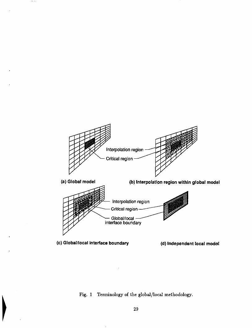
I Terminology
I The terminology of the global/local methodology presented herein is depicted in figure 1 I
to illustrate the components of the analysis procedure. The global model, figure la, is a finite
element model of an entire structure or a subcomponent of a structure. A region requiring a
more detailed interrogation is subsequently identified by the structural analyst. This region
may be obvious, such as a region around a cutout in a panel, or not so obvious, such as a
local buckled region of a curved panel loaded in compression. Because the location of these
regions are usually unknown prior to performing the global analysis, the structural analyst
must develop a global model with sufficient detail to represent the global behavior of the
structure. An interpolation region is then identified around the critical region as indicated in
figure lb. An interpolation procedure is used to determine the displacements and rotations used as “boundary conditions” for the local model. The interpolation region is the region within
which the generalized displacement solution will be used to define the interpolation matrix. The
global/local interface boundary, indicated in figure IC, coincides with the intersection of the boundary of the local model with the global model. The definition of the interface boundary may affect the accuracy of the interpolation and thus the local stress state. The local model
lies within the interpolation region as shown in figure IC and is generally more refined than the global model in order to predict more accurately the detailed state of stress in the critical
region. However, the local model is independent of the global finite element model as indicated
in figure Id. The coordinates or nodes of the local model need not be coincident with any of the
coordinates or nodes of the global model.
The global/local interpolation procedure consists of generating a matrix based on the
global solution and a local interpolated field. The local interpolated field is that field which is
interpolated from the global analysis and is valid over the domain of the local model. Local
stress analysis involves the generation of the local finite element model, use of the interpolated
field to impose boundary conditions on the local model, and the detailed stress analysis.
Global Modeling and Analysis
I , The development of a global finite element moclel of an aerospace structure for accuratc
stress predictions near local discontinuities is often too time consuming to impact the design
and certification process. Predicting the global structural response of these structures often has
many objectives including overall structural response, stress analysis, and determining internal
load distributions. Frequently, structural discontinuities such as cutouts are only accounted for in
6
the overall sense. Any local behavior is then obtained by a local analysis, possibly by another
analyst. The load distribution for the local region is obtained from the global analysis. The local model is then used to obtain the structural behavior in the specified region. For example,
the global response of an aircraft wing is obtained by a coarse finite element analysis. A typical
subcomponent of the wing is a stiffened panel with a cutout. Since cutouts are known to produce
high stress gradients, the load distributions from the global analysis of the wing are applied to
the stiffened panel to obtain the local detailed stress state. One difficulty in modeling cutouts
is the need for the finite element mesh to transition from a circular pattern near the cutout to a rectangular pattern away from the cutout. This transition region is indicated in figure 2 and will be referred to as a transition square ( i . e . , a square region around the cutout used to
transition from rings of elements to a rectangular mesh). This transition modeling requirement
impacts both the region near the cutout and the region away from the cutout. Near the cutout,
quadrilateral elements may be skewed, tapered, and perhaps have an undesirable aspect ratio. In addition, as the mesh near the cutout is refined by adding radial “spokes” of nodes and
“rings” of elements, the mesh away from the cutout also becomes refined. For example, adding
radial spokes of nodes near the cutout also adds nodes and elements in the shaded regions (see
figure 2) away from the cutout. This approach may dramatically increase the computational
requirements necessary to obtain the detailed stress state. Alternate mesh generation techniques
using transition zones of triangular elements or multipoint constraints may be used; however, the
time spent by the structural analyst will increase substantially.
The global modeling herein, although coarse, is sufficient to represent the global structural
behavior. The critical regions have been modeled with only enough detail to represent their effect on the global solution. This modeling step is one of the key components of the global/local methodology since it provides an “adequate” global analysis. Although the critical regions are known for the numerical studies discussed in a subsequent section, this a priori knowledge is not
required but may be exploited by the analyst.
Local Modeling and Analysis
The local finite element modeling and analysis is performed to obtain a dctailed analysis
of the local structural region(s). The local model accurately represents the geometry of the structure necessary to provide the local behavior and stress state. The discretization
requirements for the analysis are governed by the accuracy of the solution desired. The
discretization of the local model is influenced by its proximity to a high stress gradient.
7
One approach for obtaining the detailed stress state is to model the local region with an
arbitrarily large number of finite elements. Higher-order elements may be usell to reduce the number of elements requircd. Detailed refinement is much more advantageous for use in the
local model than in the global model. The local refinement affects only the lo(.al model, unlike
embedding the same refinement in the global model which would propagate to regions not requiring such a level of detailed refinement. A second approach is to refine the model based
on engineering judgement. Mesh grading, in which smaller elements are used near the gradient,
may be used. An error measure based on the change in stresses from element to element may be used to determine the accuracy in the stress state obtained by the initial l c d finite element
mesh. If the accuracy of the solution is not satisfactory, additional refinement j are required. The
additional refinements may be based on the coarse global model or the displacement field in the
local model which suggests a third approach. The third approach is a multi-level global/local analysis. At the second local model level, any of the three approaches discussc d may be used to
obtain the desired local detailed stress state. Detailed refinement is used for local modeling in
this study.
Global/Local Interface Boundary Definition
The definition of the global/local interface boundary is problem dependent. Herein, the
location of the nodes on the interface boundary need not be coincident with any of the nodes
in the coarse global model. Reference [7] concluded that the distance that the local model must
extend away from a discontinuity is highly dependent upon the coarse model used. The more
accurate the coarse model displacement field is, the closer the local model boundary may be to the discontinuity. This conclusion is based on the results of a study of a flat, isotropic panel with
a central cutout subjected to uniform tension, but it extends to other structures with high stress
gradients.
Stresses are generally obtained from a displacement-based finite element analysis by
differentiation of the displacement field. For problem with stress gradients, the element
stresses vary from element to element, and in some cases this change, Au, may be substantial. The change in stresses, Au, may be used as a measure of the adequacy of the finite element
I discretization. Large Au values indicate structural regions where more modeling refinement is
needed. Based on this method, structural regions with small values of Au have obtained uniform
stress states away from any gradients. Therefore, the global/local interface boundary should
be defined in regions with small values of Aa (ic., away from a stress gradient). Exploratory
studies to define an automated procedure for selecting the global/local interface boundary have been performed using a measure of the strain energy. The strain energy per unit area is selected since it represents a combination of all the stress components instead of a single stress
component. Regions with high stress gradients will also have changes in this measure of strain
energy from element to element.
Global/Lo cal Interpolation Procedure
The global/local analysis method is used to determine local, detailed stress states using
independent, refined local models which exploit information from less refined global models. A two-dimensional finite element analysis of the global structure is performed to obtain its overall
behavior. A critical region may be identified from the results of the global analysis. The global
solution may be used to obtain an applied displacement field along the boundary (;.e., boundary
conditions) of an independent local model of the critical region. This step is one of the key
components of the global/local methodology; namely, interpolation of the global solution to obtain boundary conditions for the local model.
Many interpolation methods are used to approximate functions (e.g., ref. [14]). The
interpolation problem may be stated as follows: given a set of function values fj at n coordinates (z;, y;), determine a “best-fit” surface for these data. Mathematically, this problem can be stated
as
where S(ti,yi) is a matrix of interpolated functions evaluated at n points, the array a defines
the unknown coefficients of the interpolation functions, and the array f consists of known values
of the field being interpolated based on n points in the global model. Common interpolation
methods include linear interpolation, Lagraiigiaii iiileryolatioii and least-squares techniques for
polynomial interpolation. Elementary linear interpolation is perhaps the simplest method and
is an often used interpolation method in trigonometric and logarithmic tables. Another method
is Lagrangian interpolation which is an extension of linear interpolation. For this method, data
for n points are specified and a unique polynomial of degree n - 1 passing through the points
can be determined. However, a more common method involving a least-squares polynomial fit
minimizes the the sum of the square of the residuals. The drawbacks of least-squares polynomial
fitting include the requirement for repeated solutions to minimize the sum of the residual, and
the development of an extremely ill-conditioned matrix of coefficients when t l ~ e degree of the
approximating polynomial is large. A major limitation of the approximating 1 olynomials which fit a given set of function values is that they may be excessively oscillatory between the given
points or nodes.
Mat hematical Formulation of Spline Interpolation
Spline interpolation is a numerical analysis tool used to obtain the “best” local fit through a
set of points. Spline functions are piecewise polynomials of degree m that are connected together
at points called knots so as to have m - 1 continuous derivatives. The mathematical spline
is analogous to the draftman’s spline used to draw a smooth curve through a itumber of given
points. The spline may be considered to be a perfectly elastic thin beam resti:ig on simple supports at given points. A surface spline is used to interpolate a function of I wo variables and removes the restriction of single variable schemes which require a rectangitlar array of
grid points. The derivation of the surface spline interpolation function used herein is based on the principle of minimum potential energy for linear plate bending theory. This approach incorporates a classical structural mechanics formulation into the spline interpolation procedure in a general sense. Using an interpolation function which also satisfies the linear plate bending
equation provides inherent physical significance to a numerical analysis technique. The spline interpolation is used to interpolate the displacements and rotations from a global analysis
and thereby provides a functional description of each field over the domain. The fields are
interp Jlated separately which provides a consistent basis for interpolating glol la1 solutions based
on a plate theory with shear flexibility effects incorporated. That is, the out-of-plane deflections
and the bending rotations are interpolated independently rather than calculat, tng the bending rotations by differentiating the interpolated out-of--plane deflection field.
The spline interpolation used herein is derived following the approach described by Harder
and Desmairis in reference [15]. A spline surface is generated based on the solution to the linear
isotropic plate bending equation
DV4w I= q. (2)
Extensions have been made to the formulation presented in reference [15] to include higher-
order polynomial terms (underlined terms in equation (3)). The extended Cai tesisn form which
satisfies equation (2) is written as
10
where 2
Tf = ( x - X i ) + ( y - y;)2 (4)
and z i , y i are the coordinates of the i-th node in the interpolation region. The higher-order
polynomial terms were added to help represent a higher-order bending response than was being
approximated by the natural logarithm term in the earlier formulation. The additional terms
increase the number of unknown coefficients and constraint equations to n + 10. The n + 10
unkiiowns (a0 , a1 , a2,. . . , as, F;) are found from equation (3) and by solving the set of equations:
n n
i= 1 i=l
n n
i= 1 i=l
n n
i= 1 n
i=l n
i= 1 i= 1 n n
i= 1 i= 1
The constraint equations given in equation ( 5 ) are used to prevent equation (2) from becoming unbounded when expressed in Cartesian coordinates. The modified matrix equations, still of the
11
form Sa = f, are
0 0 0 ... 0 1 1 ... 1
0 0 0 ... 0 y1 Y2 Yn
0 0 0 ... 0 21 2 2 ... X n
0 0 0 ... 0 xq 2; ... x;
0 0 0 ... 0 z; x; ... x; 0 0 0 ... 0 xqy1 x;y2 ... X n Y n
0 0 0 ... 0 zly: X I Y , ~ xnyn 0 0 0 ... 0 y; y; ... Yn
where R i j = T ; ~ In(T:j + E ) for i , j = 1,2 , . . . , n and E is a parameter used to insure numerical stability for the case when ~ i j vanishes. The extended local interpolation function is similar to
equation (3) except that it is evaluated at points along the global/local interface boundary. That
is, fi = a0 + a1xi + a2yi + a3xi2 + a 4 ~ i y i + a5yi2 + agxi3 + a7si2yi+
n
a8ziyi2 + a9yi3 + F ~ T : ~ ln(r:j>; i = 1,2, ..., 1 (7) j=1
Upon solving equation (6) for the coefficients (ao, al, a2, . . . , as, Fj), equation (7) is used to
compute the interpolated data at the required local model nodes. I
Computational Strategy
A schematic which describes the overall solution strategy is shown in figure 3. The
computational strategy described herein is implemented through the use of the Computational
Structural Mechanics (CSM) Testbed (see refs. [16] and [17]). The CSM Testbed is used I to model and analyze both the global and local finite element models of a structure. Two
computational modules or processors were developed to perform the global/local interpolation
procedure. Processor SPLN evaluates the spline coefficient matrix [ S ( z i , yi)]. Processor INTS solves for the interpolation coefficients a = {a; Fi) and performs the local interpolation to obtain
the “boundary conditions” for the local model. Various other Testbed processors are used in the
12
stress analysis procedure. The overall computational strategy for the global/local stress analysis
methodology is controlled by a high-level procedure written using the command language of
the Testbed (see ref. [17]). The command language provides a flexible tool for performing
computational structural mechanics research.
Numerical Results
The effectiveness of the computational strategy for the global/local stress analysis outlined
in the previous sections is demonstrated by obtaining the detailed stress states for an isotropic
panel with a cutout and a blade-stiffened graphite epoxy panel with a discontinuous stiffener.
The first problem was selected to verify the global/local analysis capabilities while the second
problem was selected to demonstrate its use on a representative aircraft subcomponent. The
objectives of these numerical studies are:
1. To demonstrate the global/local stress analysis methodology, and
2. To obtain and interrogate the detailed stress states of representative subcomponents of
complete aerospace structures.
All numerical studies were performed on a Convex C220 minisupercomputer. The
computational effort of each analysis is quantified by the number of degrees of freedom used in
the finite element model, the computational time required to perform a stress analysis, and the
amount of auxiliary storage required. The computational time is measured in central processing
unit (CPU) time. The amount of auxiliary storage required is measured by the size of the data
library used for the input/output of information to a disk during a Testbed execution.
Isotropic Panel with Circular Cutout
An isotropic panel with a cutout is an ideal structure to verify the global/local computational strategy, since closed-form elasticity solutions axe available. Elasticity solutions
for an infinite isotropic panel with a circular cutout (e.g., ref. [IS]), predict a stress concentration
factor of three at the edge of the cutout. The influence of finite-width effects on the stress
concentration factors for isotropic panels with cutouts are reported in reference [19]. By including finite-width effects, the stress concentration factor is reduced from 1 he value of three
for an infinite panel.
The global/local linear stress analysis of the isotropic panel with a circular cutout shown
in figure 4 has been performed. The overall panel length L is 20 in., the overall width W is
13
10 in., the thickness h is .1 in, and the cutout radius T O is 0.25 in. This geometry gives a cutout diameter to panel width ratio of 0.05 which corresponds to a stress concentration factor of 2.85
(see ref. [19]). The loading is uniform axial tension with the loaded ends of the panel clamped
and the sides free. The material system for the panel is aluminum with a Young’s modulus of
10,000 ksi and Poisson’s ratio of 0.3.
Global Analysis
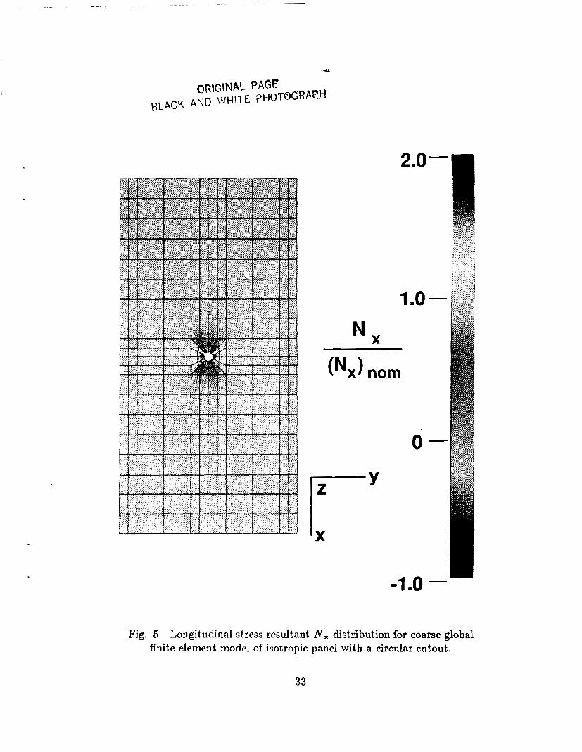
The finite element model shown in figure 4 of the isotropic panel with a circular cutout is a
representative finite element model for representing the global behavior of the panel as well as
a good approximation to the local behavior. The finite element model shown In figure 4, will be
referred to as the “coarse” global model or Model G1 in Table 1. The finite element model has a
total of 256 4-node quadrilateral elements, 296 nodes, and 1644 active degrees of freedom for the linear stress analysis. This quadrilateral element corresponds to a flat C is based on a displacement formulation and includes rotation about the outward normal axis.
Originally developed for the computer code STAGS (see refs. [20,21]), this element has been installed in the CSM Testbed software system and denoted ES5/E410 (see ref. [IS]).
shell element which
The longitudinal stress resultant N, distribution shown in figure 5 reveals several features of
the global structural behavior of this panel. First, away from the cutout, the Y, distribution in
the panel is uniform. Secondly, the N , load near the center of the panel is much greater than the
N, load in other portions of the panel due to the redistribution of the N, loall as a result of the
cutout. Thirdly, the N, load at the edge of the cutout at the points ninety dc,grees away from
the stress concentration is small relative to the uniform far-field stress state.
The distribution of the longitudinal stress resultant N, at the panel midlength normalized
by the nominal stress resultant is shown in figure 6 as a function of the distance from the cutout
normalized by the cutout radius. The results indicate that high inplane stresses and a high
gradient exist near the cutout. However, a stress concentration factor of 2.06 is obtained from
a linear stress analysis using the “coarse” finite element model (see figure 4). This value is 28%
lower than the theoretical value of 2.85 reported in reference [19]. Therefore, even though the
overall global response of the panel is qualitatively correct as indicated by the stress resultant
contour in figures 5, the detailed stress state near the discontinuity is inaccurate.
Accurate detailed stress distributions require a finite element mesh that is substantially more
refined near the cutout. Adding only rings of elements (Model G2 in Table 1) does not affect the
discretization away from the cutout; however, the stress concentration factor is still 22% lower
14
than the theoretical value. To obtain a converged solution for the stress concentration factor, a
sequence of successively refined finite element models were developed by increasing the number
of radial spokes of nodes and rings of elements in the region around the cutout. A converged
solution is obtained using a total of 3168 4-node quadrilateral shell elements (ES5/E410) in the
global model (Model G4 in Table 1). Using an intermediate refined finite element model with
a total of 832 4-node quadrilateral elements, 888 nodes, and 5156 active degrees of freedom, a
stress concentration factor of 2.72 is obtained which is within 4.6% of the theoretical solution.
This finite element model is referred to as the “refined” global model or Model G3 in Table 1.
Normalized longitudinal stress resultant N, distributions are shown in figure 6 for the “coarse”
global model (Gl) and the “refined” global model (G3). The stress gradient for this panel
becomes nearly zero at a distance from the center of the panel of approximately six times the
cutout radius.
The distribution of the strain energy for Model G1 is shown in figure 7. The change in the
strain energy per unit area within the transition square indicates that a high $tress gradient
exists near the cutout and rapidly decays away from the cutout. These results are consistent with the structural analyst’s intuition, and the local analyses described subsequently will further
interrogate the region near the cutout.
Local Analyses
A global/local analysis capability provides an alternative to global mesh refinement and
a complete solution using a more refined mesh. For this example, the “critical” region is well
known and easily identified by even a casual examination of the stress resultant distributions
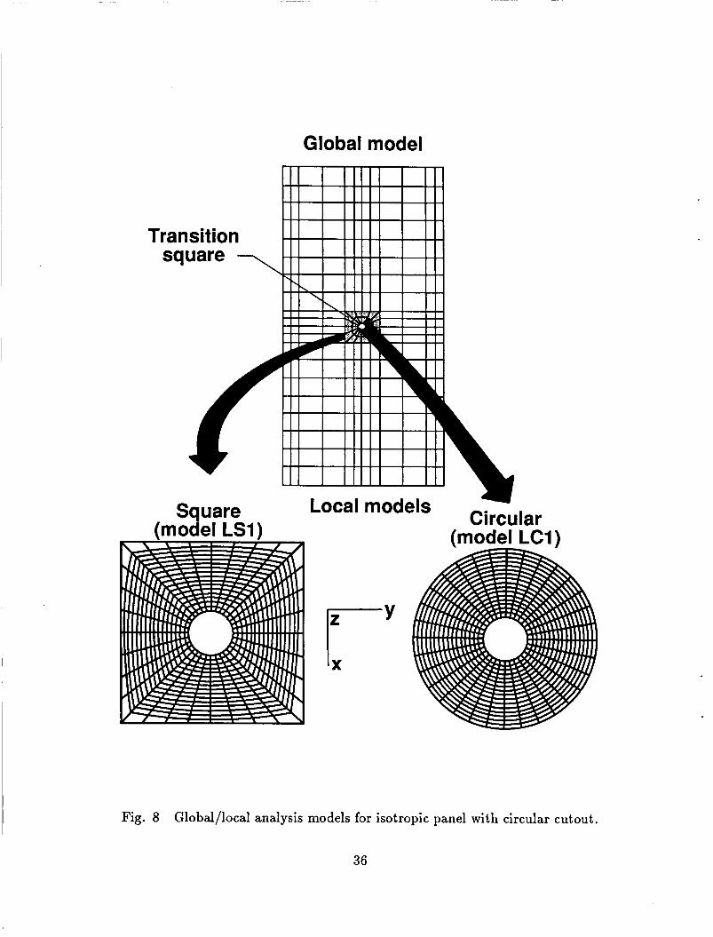
given in figure 5. The global model, the interpolation region and the local models considered are shown in figure 8. The global model corresponds to the “coarse” global model (Gl) and
the shaded region corresponds to the interpolation region which is used to generate the spline coefficient matrix and to extract boundary conditions for the local model. As indicated in figure
8, two different local models are considered: one square and one circular. Both local models
completely include the critical region with the stress concentration. The boundary of the square
local model coincides with the boundary of the transition square in the global model. The
boundary of the circular model is inscribed in the transition square. That is, the outer radius of
the circular model is equal to half the length of a side of the transition square. Both local models
(Models LS1 and LC1 in Table 1) have the same number of 4-node quadrilateral shell elements
(512), nuxnber of nodes (544) and number of degrees of freedom (3072). Both local models have
only 62% of the elements used in the refined global analysis. The global/local interpolation for
15
both local models is performed from the data obtained from the “coarse” global model analysis.
The radius of the interpolation region RI is 5.7~0 which includes the 48 data points within the
transition square of the coarse global model.
The distribution of the longitudinal stress resultant N , at the panel midlength normalized
by the nominal stress resultant obtained using the square local model is shown in figure 9a as
a function of distance from the cutout normalized hy the cutout radius. These results indicate
that the global/local analysis based on the coarse global solution and the square local model
accurately predicts the stress concentration factor at the cutout as well as the distribution at the global/local interface boundary. A stress concentration factor of 2.76 is obtained which is within
1.5% of the “refined” global model (G3) solution arid 3.2% of the theoretical solution. A contour plot of the longitudinal stress resultant distribution is given in figure 9b and indicates that the local solution correlates well overall with the global solution shown in figure 5.
The distribution of the longitudinal stress resultant N , at the panel midlength normalized
by the nominal stress resultant obtained using the circular local model is shown in figure 10a as
a function of distance from the cutout normalized by the cutout radius. These results indicate that the global/local analysis based on the coarse global solution and the circiilar local model
accurately predicts the stress concentration factor at the cutout. A stress concentration factor
of 2.75 is obtained which is within 1.5% of the “refined” global model (G3) solution and 3.2% of the theoretical solution. At the global/local interface boundary, the results from the circular local Todel differ slightly from the results obtained from the refined globid model analysis.
This Jifference is attributed to interaction between the “coarse” global model, the interpolation region, and the location of the global/local interface boundary. A contour plot of the longitudinal
stress resultant distribution is given in figure 10b and indicates the overall correlation with the
distributions obtained using the global models.
The interaction between the global model, the interpolation region, and the location of the
global/local interface boundary is now assessed. This assessment involves refining the global
model in the transition square, varying the radius of the interpolation region R I and varying
the radius of the local model RL. Using an interpolation region defined as RI = 14~0 (72 data
points from the global model), several local models are considered in which R 1, is increased from
twice the cutout radius to five times the cutout radius. The results in figure 1 la are based on
using the coarse global model (Gl) for the global solution. These results indicate that the local
solution deteriorates as the global/local interface boundary is moved closer to the cutout. The
results in figure l l b are based on a slightly more refined global model(G2) for the global solution.
16
This global model has two additional rings of elements in the transition square. Comparing the
results in figures l l a and l l b reveals the interaction between the global model and the location of the interface boundary. To obtain an accurate local solution for the case when the global/local
interface boundary is located within a region with a high stress gradient requires that sufficient
data from the global model be available in the area to provide accurate “boundary conditions”
for the local model. These results indicate that by adding just two rings of elements near the
cutout (Model G2), the extraction of the local model boundary conditions from the spline
interpolation is improved such that the global/local interface boundary may be located very near
the cutout.
The influence of the radius of the interpolation region on the local solution was determined to be minimal provided the global model discretization is adequate. For the cases considered,
identical local solutions are obtained using an interpolation region larger than the local model or
an interpolation region which coincides with the local model.
Computational Requirements
A summary of the computational requirements for the global and local analyses of the
isotropic panel with the circular cutout is given in Table 2. The computational cost in central
processing unit (CPU) seconds of the local analyses is approximately 74% of the CPU time of the
refined global analysis. The CSM Testbed data libraries for the local analyses are 59% smaller
than the data library for the refined global analysis. The local models have 60% and 16% of the
total number of degrees of freedom required for the refined model ( G 3 ) and converged global
model (G4), respectively.
Usage Guidelines
Usage guidelines derived from the global/local analysis of the isotropic panel with a circular
cutout are as follows. An “adequate” global analysis is required to ensure a sufficient number
of accurate data points to provide accurate “boundary conditions” for the local model. When
the global/local interface boundary, RL is within the high stress gradient (ie., within a distance
of two times the cutout radius from the cutout edge), the importance of an “adequate” global analysis in the high gradient region is increased. The interpolation region should coincide with
or be larger than the local model. To satisfy the compatibility requirements at the global/local
interface boundary, the local model boundary RL sliould be defined sufficiently far from the
cutout ( L e . , a distance of approximately six times the radius from the cutout).
17
Composite Blade-Stiffened Panel with Discontinuous Stiffener
Discontinuities and eccentricities are common in aircraft structures. For example, the
lower surface of the Bell-Boeing V-22 tilt-rotor wing structure has numerous cutouts and
discontinuous stiffeners (see figure 12). Predicting the structural response of such structures
in the presence of discontinuities, eccentricities, and damage is particularly difficult when the component is built from graphite-epoxy materials or is loaded into the nonlinear range.
In addition, potential damage of otherwise perfect structures is often an important design
consideration. Recent interest in applying graphite-epoxy materials to aircraft primary structures has led to several studies of postbuckling behavior and failure characteristics of
graphite-epoxy components (e.g., ref. [22]). One goal of these studies has been the accurate
prediction of the global response of the composite structural component in the postbuckling
range. In one study of composite stiffened panels, R blade-stiffened panel was tested (see ref.
[23]). A composite blade-stiffened panel was proof-tested and used as a “control specimen”. The
panel was subsequently used in a study on discontiriuities in composite blade-stiffened panels. The global structural response of these composite blade-stiffened panels presented in reference
[24] correlate well with the earlier experiment data. The composite blade-stiffened panel with a discontinuous stiffener shown in figure 13 is representative of an typical aircraft structural
component and will be used to demonstrate and assess the global/local methodology. This problem was selected because it has characteristics which often require .a globsl/local analysis.
These characteristics include a discontinuity, eccentric loading, large displacements, large stress
gradients, high inplane loading, and a brittle material system. This problem represents a generic
class of laminated composite structures with discoiitixiuities for which the interlaminar stress
state becomes important. The local and global finite element modeling and analysis needed to
predict accurately the detailed stress state of flat blade-stiffened graphite-epoxy panels loaded in
axial compression is described in this section.
The overall panel length L is 30 in., the overall width W is 11.5 in., the stiffener spacing b is 4.5 in., the stiffener height h, is 1.4 in., and the cutout radius T O is 1 in. The three blade-shaped
stiffeners are identical. The loading is uniform axial compression. The loaded ends of the panel are clamped and the sides are free. The material system for the panel is T300/5208 graphite-
epoxy unidirectional tapes with a nominal ply thickness of 0.0055 in. Typical lamina properties
for this graphite-epoxy system are 19,000 ksi for the longitudinal Young’s modulus, 1,890 ksi for
the transverse Young’s modulus, 930 ksi for the shear modulus, and 0.38 for the major Poisson’s
18
ratio. The panel skin is a 25-ply laminate ([f45/02/ F 45/03/ f 45/03/ and the blade stiffeners are 24-ply laminates ([f45/020/
45/03/ f 45/02/ 7 451)
451).
End-shortening results are shown in figure 14 for the ‘‘control specimen” and for the
configuration with a discontinuous stiffener. These results indicate that the presence of the
discontinuity markedly changes the structural response of the panel. The structural response
of the “control specimen” is typical of stiffened panels. Two equilibrium configurations are
exhibited; namely, the prebuckling configuration and the postbuckling configuration. The structural response of the configuration with a discontinuous stiffener is nonlinear from the onset
of loading due to the eccentric loading condition and the cutout. The blade-stiffened panel with
a discontinuous stiffener was tested to failure. Local failures occurred prior to overall panel failure as evident from the end-shortening results shown in figure 14.
Global Analysis
A global linear stress analysis of the composite blade-stiffened panel with a discontinuous
stiffener was performed for an applied load corresponding to P / E A of 0.0008 (ie., an applied compressive load P of 19,280 pounds normalized by the extensional stiffness EA) . At this load
level, the structural response of the panel is essentially linear. Out-of-plane deflections are
present, however, due to thc eccentric loading condition caused by the discontinuous stiffener.
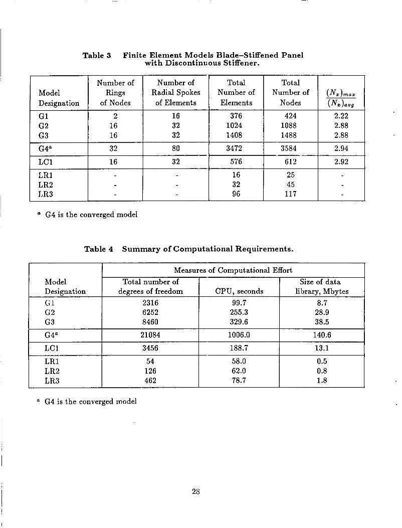
Several global finite element models are considered as indicated in Table 3 to obtain a converged
solution for comparison purposes since a theoretical solution is not available. The value of the
longitudinal stress resultant at the edge of the cutout changed less than 2% between Models G2 and G4. Therefore, Model G1 will be referred to as the “coarse” global model (see figure 15), Model G2 will be referred to as the “refined” global model, and Model G4 will be referred to as the “converged” global model.
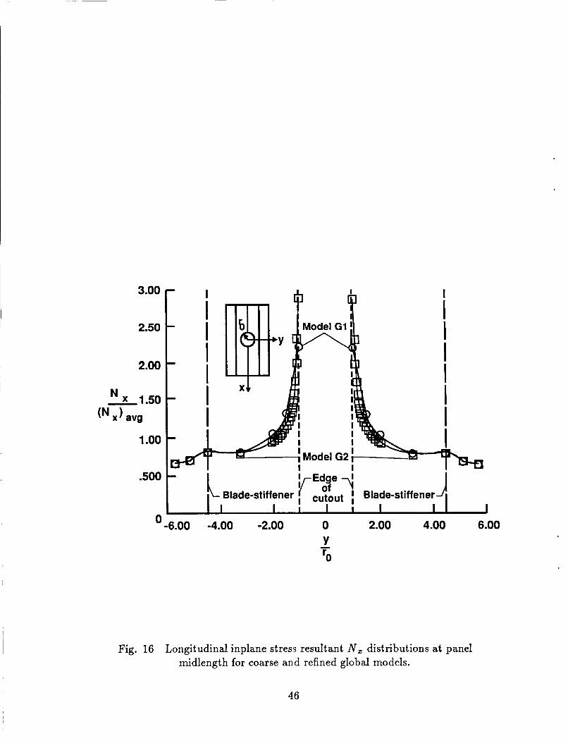
The distribution of the longitudinal stress resultant N, normalized by the average applied
running load ( N z ) a v g (ie., applied load divided by the panel width) as a function of the lateral
distance from the center of the panel normalized by the radius of the cutout is shown in figure
16 for both the “coarse” (Gl) and the “refined” (G2) global models. These results are similar to those obtained for the isotropic panel with a cutout. The maximum longitudinal stress
resultants (N,),, , normalized by the average applied running load (Nr)avg are given in Table 3. The results obtained using the coarse global model adequately represent the distribution away
from the discontinuity but underestimate (by 24%) the stress concentration at the edge of the
discontinuity.
19
An oblique view of the deformed shape with exaggerated deflections is shown in figure 17 for the coarse global model. A contour plot of the longitudinal inplane stress resultant N , is also
shown in this figure. The distribution indicates that the model provides good overall structural
response characteristics. The N , distribution reveals several features of the global structural
behavior of this panel. First, away from the disconlinuity, the N , distribution in the panel skin
is nearly uniform and approximately half the value of the N , in the outer two blade stiffeners.
Second, load is diffused from the center discontinuous stiffener into the panel skin rapidly such
that the center stiffener has essentially no N , load at the edge of the cutout. Third, the N , load
in the outer stiffeners increases towards the center of the panel and is concentrated in the blade
free edges ( L e . , away from the stiffener attachment line at the panel skin). Fourth, the N , load
in the panel skin near the center of the panel is much greater than the N , load in other portions
of the panel skin.
The distribution of the strain energy for Model G1 is shown in figure 18. The change in
the strain energy per unit area within the transition square again indicates that a high stress
gradient exists near the discontinuity and rapidly decays away from the discontinuity. These results are consistent with the structural analyst’s intuition, and the local models described
subsequently will further interrogate the region near the discontinuity. For this load level, the
skin-stiffener interface region has not yet become heavily loaded. However, this region will also
be studied further to demonstrate the flexibility of the global/local stress analysis procedure
presented herein.
Local Analyses
A global/local analysis capability provides an alternative approach to glolial mesh refinement
and a complete solution using a more refined mesh. For this example, one “critical” region
is easily identified by even a casual examination of the stress resultant distribution given in
figure 17. A second critical region that may require further study is indicated by the slight
gradient near the intersection of the outer blade-stiffeners and the panel skin at the panel
midlength as shown in figure 17. Skin-stiffener separation has been identified as a dominant failure mode for stiffened composite panels (see ref. [22]). The global model, the interpolation
regions and the local models considered are shown in figure 19. The global model corresponds to
the “coarse” global model (Gl) and the shaded regions correspond to the interpolation regions
which are used to generate the spline coefficient matrix and to extract boundary conditions for
the local model. As indicated in figure 19, two different critical regions are considered. One
region is near the discontinuity and a circular local model is used. The boundary of the circular
20
model is inscribed in the transition square. That is, the outer radius of the ci. cular model is
equal to half the length of a side of the transition square. The other region is near the skin-
stiffener interface region at the panel midlength for one of the outer stiffeners. The global/local interpolation for the local models is performed front the data obtained from the “coarse” global
model analysis. Two interpolation regions were used in each of the local analyses. The first interpolation region, specified in the plane of the panel skin, is used to obtain the boundary
conditions on the global/local interface boundary of the panel skin. The second interpolation
region, specified in the plane of the stiffener, is used to obtain the boundary c*,nditions on the
global/local interface boundary of the stiffener. The boundary conditions for i he panel skin and
the stiffener’ were interpolated separately. Compatibility of displacements and rotations at the
skin-stiffener intersection on the global/local interface boundaries was enforced by imposing the boundary conditions obtained for the panel skin.
The local model (Model LC1 in Table 3) of thc: first critical region near t ; te discontinuity
has 576 4-node quadrilateral shell elements, 612 nodes, and 3456 degrees of frc edom. This local
model has only 56% of the elements used in the refined global analysis. The distribution of the
longitudinal stress resultant N , at the panel midlength normalized by the average running load (Nz )avg is shown in figure 20a as a function of the lateral distance from the cutout normalized by
the cutout radius. These results indicate that the global/local analysis based on the coarse global
solution accurately predicts the stress concentration at the cutout as well as the distribution at the global/local interface boundary. A contour plot of the longitudinal stress resultant
distribution is given in figure 20b. The results indicate that the local solution correlates well with
the global solutions shown in figure 17.
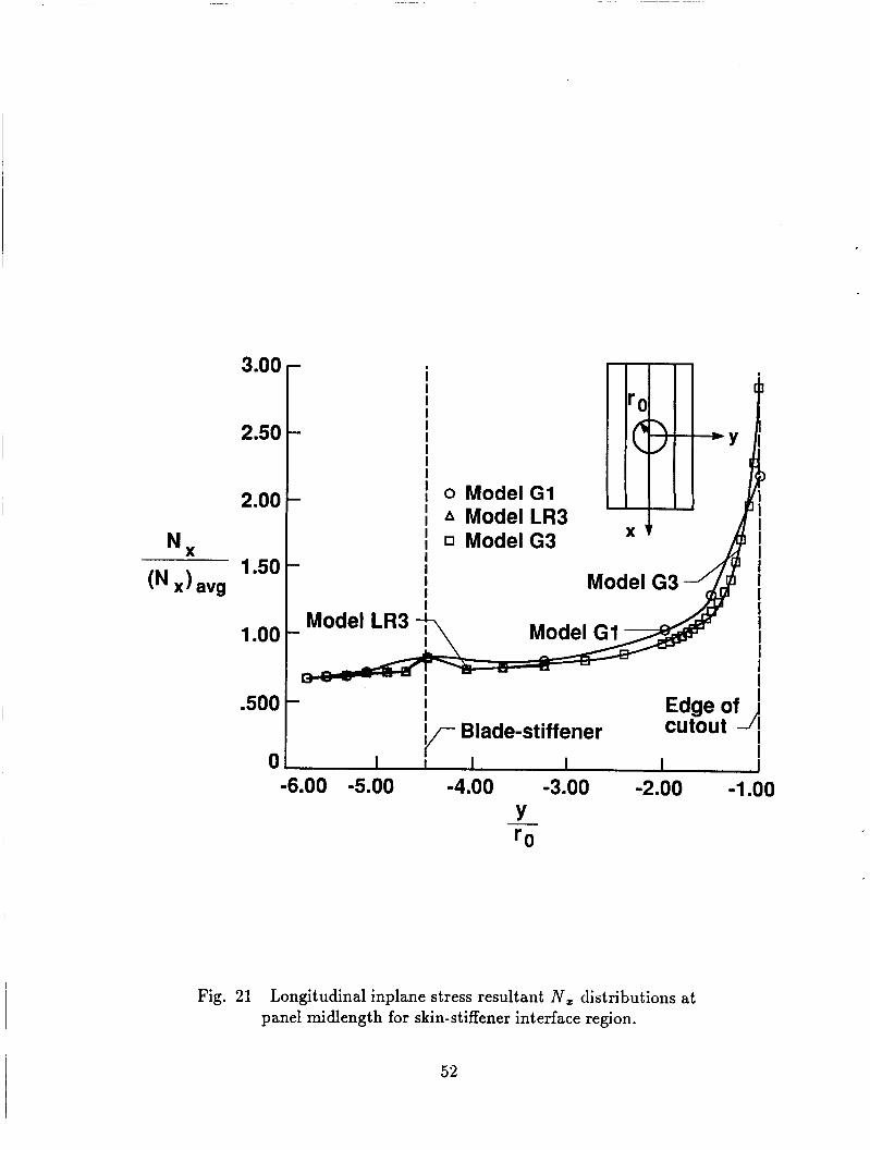
The second critical region near the intersection of the outer blade-stiffener and the pariel
skin at the midlength is studied further. Three cliffcrent local finite element n odels of this
critical region arc considered as indicated in Table 3. The first, Model LRl, 11,~s the same nuniber
of nodes (25) and number of elements (16) within the critical region as the coarse global model
(Gl). The second, Model LR2, has the same number of nodes (45) and number of elements (32)
within the critical region as the refined global model (G2). The third and most refined model,
Model LR3, has 117 nodes, 96 elements and 462 degrees of freedom. The longitudinal stress
resultant N , distributions obtained for the local models (LR1 and LR2) correlate well with the
NE distributions for the coarse and refined global models (Models G1 and G2). However, these
models are not sufficiently refined in the skin-stiRener interface region to accurately predict the
gradient at the skin-stiffener intersection. The distribution of the longitudinal stress resultant
21
N , normalized by the applied running load as a function of the lateral distance from the center of the panel normalized by the radius of the cutout is shown in figure 21. These results indicate
that the global/local analysis using the local model Model LR3 predicts a higher gradient at = -4.5 in the skin-stiffener interface region than the other global and local analyses. A
To
third global model Model G3 is used to investigate the local structural behavior predicted by
Model LR3. The global analysis performed with Model G3 predicts the same local behavior as
the analysis performed with Model LR3 as indicated in figure 21. Several factors should be borne
in mind. First, the local analysis revealed local behavior at the skin-stiffener interface region that was not predicted by either of the global models. Second, the global modeling requirement
for examining the skin-stiffener interface region are substantial. Because the c;lobal models were
generated to predict the stress distribution around the discontinuity, additiond radial “spokes” in the transition square are required to refine the panel skin in the skin-stiffel er interface region
in the longitudinal direction. Third, the global/local analysis capability provi(1es the analyst with
the added modeling flexibility to obtain an accurate detailed response at multiple critical regions
(ie., at the discontinuity and at the skin-stiffener interface region) with mini:nal modeling and computational effort.
Computational Requirements
A summary of the computational requirements for the global and local analyses of the
graphite-epoxy blade-stiffened panel with the discontinuous stiffener is given in Table 4. The computational cost in CPU seconds of the local analyses around the discontinuity is
approximately 57% of the CPU time of the refined global analysis. The CSM Testbed data
libraries for the local analyses are half of the size of the data library for the refined global
analysis. The local models have 55% and 16% of the total number of degrees of freedom required
for the refined model (G2) and converged global model (G4), respectively. The CPU time for the refined local analysis (LR3) of the skin-stiffener interface region is 24% of the CPU time required
for the global analysis with Model G3. The size of the data library for the 10c.d analysis is 5% of
the size of the data library required for the analysis with Model G3.
UsaEe Guidelines
Usage guidelines derived from the global/local analysis of the blade-stiffened panel with
a discontinuous stiffener are as follows. An “adequate” global analysis is required to ensure a
sufficient number of accurate data points to provide accurate “boundary conditions” for the
local model. When the global/local interface boundary, R L is within the high stress gradient
22
( i .e . , within a distance of two times the cutout radius from the cutout edge), the importance
of an “adequate” global analysis in the high gradie1,t region is increased. The interpolation region should coincide with or be larger than the local model. To satisfy the compatibility
requirements at the global/local interface boundary, the local model boundary RL should be defined sufficiently far from the cutout (;.e., a distance of approximately six times the radius
from the cutout). For the blade-stiffened panel, two interpolation regions should be specified,
one for the interpolation of the boundary conditions on the boundary of the panel skin and a
second for the interpolation of the boundary conditions on the outer edges of the stiffeners.
Conclusions
A global/local analysis methodology for obtaining the detailed stress state of structural components is presented. The methodology presented is not restricted to having a priori
knowledge of the location of the regions requiring a detailed stress analysis. The effectiveness
of the global/local analysis capability is demonstrated by obtaining the detailed stress states of
an isotropic panel with a cutout and a blade-stiffened graphite-epoxy panel with a discontinuous stiffener.
Although the representative global finite element models represent the global behavior of
the structures, substantially more refined finite element meshes near the cutouts are required to
obtain accurate detailed stress distributions. Embedding a local refined model in the complete
structural model increases the computational requirements. The computational effort for the
independent local analyses is less than the computational effort for the global analyses with the
embedded local refinement.
The global/local analysis capability provides the modeling flexibility required to address
detailed local models as their need arises. This modeling flexibility was demonstrated by the local analysis of the skin-stiffener interface regions of the blade-stiffened panel with a
discontinuous stiffener. This local analysis revealed local behavior that was not predicted by the
global analysis.
The definition of the global/local interface boundary affects the accuracy of the local
detailed stress state. The strain energy per unit arca has been identified as a ineans for
identifying a critical region and the location of tile associated global/loc:al interface boundary.
The change in strain energy from element to element indicates regions with high stress gradients
( i e . , critical regions). A global/local interface boundary is defined outside of i~ region with large
changes in strain energy.
23
The global/local analysis capability presented provides a general-purpose analysis tool for use by the aerospace structural analysis community by providing an efficient strategy for accurately predicting local detailed stress states that occur in structures discretized with relatively coarse finite element models. The coarse model represents the global structural
behavior and approximates the local stress state. Independent, locally-refined finite element models are used to accurately predict the detailed stress state in the regions of interest based on
the solution predicted by the coarse global analysis.
Acknowledgements
This work represents a portion of the first author’s Master’s thesis submitted to the faculty
of the Old Dominion University. Refer e nc e s
1. Knight, Norman F., Jr.; Greene, William H.; and Stroud, W. Jefferson: Nonlinear Response of a Blade-Stiffened Graphite-Epoxy Panel with a Discontinuous Stiffener. Proceedings of NASA Workshop on Computational Methods in Structural Mechanics and Dynamics, W. J. Stroud; J. M. Housner; J. A. Tanner; and R. J. Hayduk (editors), June 19-21, 1985, NASA CP-3034 - PART 1, 1989, pp. 51-66.
2. Noor, Ahmed K.: Global-Local Methodologies and Their Application to Nonlinear Analysis. Finite Elements in Analysis and Design, Vol. 2, No. 4, December 1986, pp. 333-346.
3. Wilkins, D. J.: A Preliminary Damage Tolerance Methodology for Composite Structures. Proceedings of NASA Workshop on Failure Analysis and Mechanisms of Failure of Fibrous Composite Structures, A. K. Noor, M. J. Shuart, J. H. Starnes, Jr., and J. G. Williams !,:ompilers), NASA CP-2278, 1983, pp. 61-93.
4. €Ian, Tao-Yang; and Abel, J. F.: Computational Strategies for Nonlinear and Fracture Mechanics, Adaptive Substructuring Techniqucs in Elasto-Plastic Finite Element Analysis. Computers and Structures, Vol. 20, No. 1-3, 1985, pp. 181-192.
5. Clough, R. W.; and Wilson, E. L.: Dynamic Analysis of Large Structural Systems with Local Nonlinearities. Computer Methods in Applied Mechanics and Engineering, Vol. 17/18, Part 1, January 1979, pp. 107-129.
6. Schwartz, David J.: Practical Analysis of Stress Raisers in Solid Structures. Proceedings of the 4th International Conference on Vehicle Structural Mechanics, Warrandale, PA, Nov. 1981, pp. 227-231.
7. Kelley, F. S.: Mesh Requirements of a Stress Concentration by the Specified Boundary Displacement Method. Proceedings of the Second International Computers in Engineering Conference, ASME, Aug. 1982, pp. 39-42.
8. Griffin, 0. Hayden, Jr.; and Vidussoni, Marco A.: Global/Local Finite Element Analysis of Composite Materials. Computer-Aided Design in Composite Material Technology, C. A. Brebbia, W. P. de Wikle, and W. R. Blain (editors), Proceedings of the International
24
Conference for Computer-Aided Design in Coinposite Material Technology, Southampton, UK, April 13-15, 1988, pp. 513-524.
9. Jara-Almonte, C. C.; and Knight, C. E.: The Specified Boundary Stiffness/Force SBSF Method for Finite Element Subregion Analysis. International Journal for Numerical Methods in Engineering, Vol. 26, 1988, pp. 1!167-1578.
10. Hirai, Itio; Wang, Bo Ping; and Pilkey, Walter D.: An Efficient Zooming Method for Finite Element Analysis. International Journal for Numerical Methods in Engineering, Vol. 20, 1984, pp. 1671-1683.
11. Hirai, Itio; Wang, Bo Ping; Pilkey, Walter D.: An Exact Zooming Method. Finite Element
12. Dong, Stanley B.: Global-Local Finite Element Methods. State-Of-The-Art
Analysis and Design, Vol. 1, No. 1, April 1985, pp. 61-68.
Surveys on Finite Element Technology, A. K. Noor and W. D. Pilkey (editors), ASME, 1983, pp. 451-474.
13. Stehlin, P.; and Rankin, C. C.: Analysis of Structural Collapse by the Reduced Basis Technique Using a Mixed Local-Global Formulation. AIAA Paper No. 86-0851-CP, May 1986.
14. Gladwell, G. M. L.: Practical Approximation Theory, University of Watcrloo Press, 1974.
15. Harder, Robert L.; and Desmarais, Robert N.: Interpolation Using Surface Splines. Journal of Aircraft, Vol. 9, No. 2, February 1972, pp. 189-191.
16. Stewart, Caroline B., Compiler: The Computational Structural Mechanics Testbed User’s Manual. NASA TM-100644,1989.
17. Gillian, R. E.; and Lotts, C. G.: The CSM Testbed Software System - A Development Environment for Structural Analysis Methods on the NAS CRAY-2. NASA TM-100642 , 1988.
18. Timoshenko, S. P.; and Goodier, J. N.: Theory of Elasticity. McGraw-Hill Book Company,
19. Peterson, R. E.: Stress Concentration Design Factors. Wiley-International, New York, 1953,
New York, 1934, pp. 90-97.
pp. 77-88.
20. Alnlroth, B. 0.; and Brogan, F. A.: The STAGS Computer Code. NASA CR-2950,1978.
21. Almroth, B. 0.; Brogan, F. A.; and Stanley, G. M.: Structural Analysis of General Shells - Volume 11: User Instructions for STAGSC-1. NASA CR-165671, 1981.
22. Starnes, James H., Jr.; Dickson, John N.; and Rouse, Marshall: Postbuckling Behavior of Graphite-Epoxy Panels. ACEE Composite Structures Technology: Review of Selected NASA Research on Composite Materials and Structures. NASA CP-2321, 1984, pp. 137- 159.
23. Williams, Jerry G.; Anderson, Melvin S.; Rhodes, Marvin D.; Starnes, James H., Jr.; and Stroud, W. Jefferson: Recent Developments in the Design, Testing, and Impact-Damage Tolerance of Stiffened Composite Panels. NASA TM-80077, 1979.
25
24. Knight, Norman F., Jr.; McCleary, Susan L.; Macy, Steven C.; and Aminpour, Mohammad A.: Large-Scale Structural Analysis: The Strnctural Analyst, The CSM Testbed, and The NAS System. NASA TM-100643,1989.
26
Table 1 Finite Element Models of Isotropic Panel with Circular Cutout.
Number of Rings
of Nodes
2 4
16
32
16 16
Model Designation
Number of Tot a1 Tot a1
of Elements Elements Nodes Radial Spokes Number of Number of Kt
10. Work Unit No. 9. Performing Organization Name and Address
505-63-01-10 NASA Langley Research Center Hampton, VA 23665-5225 11. Contract or Grant No.
13. Type of Report and Period Covered
Technical Memorandum 12. Sponsoring Agency Name and Addreas
National Aeronautics and Space Administration Washington, DC 20546-0001
14. Sponsoring Agency Code
19. Security Classif.(of this report) 20. Security Classif.(of this page) Unclassified Unclassified
15. Supplementary Notes Presented at the Third Joint ASCE/ASME Mechanics Conference, University of California at San Diego, Julv 9-12. 1989.
21. No. of Pages 22. Price 53 A03
~~~~
16. Abstract A method for performing a global/local stress analysis is described and its capabilities are demon-
strated. The method employs spline interpolation functions which satisfy the linear plate bending equation to determine displacements and rotations from a global model which are used as “boundary conditions” for the local model. Then, the local model is analyzed independent of the global model of the structure. This approach can be used to determine local, detailed stress states for specific structural regions using independent, refined local models which exploit information from less-refined global models. The method presented is not restricted to having a priori knowledge of the location of the regions requiring local detailed stress analysis. This approach also reduces the computational effort necessary to obtain the detailed stress state. Criteria for applying the method are developed. The effectiveness of the method is demonstrated using a classical stress concentration problem and a graphite-epoxy blade-stiffened panel with a discontinuous stiffener.