Biostatistics (2004), 5, 1, pp. 89–111 Printed in Great Britain Factorial and time course designs for cDNA microarray experiments G. F. V. GLONEK School of Applied Mathematics, The University of Adelaide, Adelaide, SA 5005, Australia P. J. SOLOMON ∗ School of Applied Mathematics, The University of Adelaide, Adelaide, SA 5005, Australia [email protected]SUMMARY Microarrays are powerful tools for surveying the expression levels of many thousands of genes simultaneously. They belong to the new genomics technologies which have important applications in the biological, agricultural and pharmaceutical sciences. There are myriad sources of uncertainty in microarray experiments, and rigorous experimental design is essential for fully realizing the potential of these valuable resources. Two questions frequently asked by biologists on the brink of conducting cDNA or two-colour, spotted microarray experiments are ‘Which mRNA samples should be competitively hybridized together on the same slide?’ and ‘How many times should each slide be replicated?’ Early experience has shown that whilst the field of classical experimental design has much to offer this emerging multi-disciplinary area, new approaches which accommodate features specific to the microarray context are needed. In this paper, we propose optimal designs for factorial and time course experiments, which are special designs arising quite frequently in microarray experimentation. Our criterion for optimality is statistical efficiency based on a new notion of admissible designs; our approach enables efficient designs to be selected subject to the information available on the effects of most interest to biologists, the number of arrays available for the experiment, and other resource or practical constraints, including limitations on the amount of mRNA probe. We show that our designs are superior to both the popular reference designs, which are highly inefficient, and to designs incorporating all possible direct pairwise comparisons. Moreover, our proposed designs represent a substantial practical improvement over classical experimental designs which work in terms of standard interactions and main effects. The latter do not provide a basis for meaningful inference on the effects of most interest to biologists, nor make the most efficient use of valuable and limited resources. Keywords: cDNA microarrays; Factorial experiments; Optimal experimental design; Time course experiments. 1. I NTRODUCTION Microarrays are powerful tools for surveying the expression levels of many thousands of genes simultaneously. They belong to the new genomics technologies which are rapidly transforming molecular biology from its historical paradigm of the identification, cloning and analysis of specific gene products. There are many different microarray technologies, ranging from the high-density nylon membrane arrays ∗ To whom correspondence should be addressed. Biostatistics 5(1) c Oxford University Press (2004); all rights reserved.
Transcript
Biostatistics(2004),5, 1,pp. 89–111Printed in Great Britain
Factorial and time course designs for cDNAmicroarray experiments
G. F. V. GLONEK
School of Applied Mathematics, The University of Adelaide, Adelaide, SA 5005, Australia
P.J. SOLOMON∗
School of Applied Mathematics, The University of Adelaide, Adelaide, SA 5005, [email protected]
SUMMARY
Microarrays are powerful tools for surveying the expression levels of many thousands of genessimultaneously. They belong to the new genomics technologies which have important applications inthe biological, agricultural and pharmaceutical sciences. There are myriad sources of uncertainty inmicroarray experiments, and rigorous experimental design is essential for fully realizing the potentialof these valuable resources. Two questions frequently asked by biologists on the brink of conductingcDNA or two-colour, spotted microarray experiments are ‘Which mRNA samples should be competitivelyhybridized together on the same slide?’ and ‘How many times should each slide be replicated?’ Earlyexperience has shown that whilst the field of classical experimental design has much to offer this emergingmulti-disciplinary area, new approaches which accommodate features specific to the microarray contextare needed. In this paper, we propose optimal designs for factorial and time course experiments, whichare special designs arising quite frequently in microarray experimentation. Our criterion for optimalityis statistical efficiency based on a new notion of admissible designs; our approach enables efficientdesigns to be selected subject to the information available on the effects of most interest to biologists,the number of arrays available for the experiment, and other resource or practical constraints, includinglimitations on the amount of mRNA probe. We show that our designs are superior to both the popularreference designs, which are highly inefficient, and to designs incorporating all possible direct pairwisecomparisons. Moreover, our proposed designs represent a substantial practical improvement over classicalexperimental designs which work in terms of standard interactions and main effects. The latter do notprovide a basis for meaningful inference on the effects of most interest to biologists, nor make the mostefficient use of valuable and limited resources.
Microarrays are powerful tools for surveying the expression levels of many thousands of genessimultaneously. They belong to the new genomics technologies which are rapidly transforming molecularbiology from its historical paradigm of the identification, cloning and analysis of specific gene products.There are many different microarray technologies, ranging from the high-density nylon membrane arrays
popular amongst medical and agricultural scientists, to the short oligonucleotide (Affymetrix) arrayswhich are more accurate, but proprietry and expensive. Our experience has been with the class of spottedcomplementary DNA (cDNA) microarrays (Brown and Botstein, 1999; Eisen and Brown, 2000) andrecently also with spotted long oligonucleotide arrays; the latter and cDNA arrays are often collectivelyreferred to as ‘two-colour’ or spotted microarrays.
Microarray experiments are conducted in many different contexts with applications ranging fromanalysing cellular responses to biological and environmental stimuli, genetic mapping studies anddiagnosing disease states, to understanding gene regulation and interactions; the key motivation forresearch in these and related fields is the expectation of rapid advance in understanding the genetic basisof disease, and hopefully, of finding cures. The interface of biology, medicine, computer science andstatistics which used to be data-poor is now data-mega-rich, and statistics has a central role to play inproducing and processing that information, and to making it intelligible.
Our paper is concerned with planning microarray experiments, a topic on which there are stillrelatively few published papers, despite the fact that rigorous experimental design is essential foraccurately measuring the effects of most interest to biologists. Kerr and Churchill (2001) is dedicatedto a discussion of classical experimental designs for microarray experiments and primarily considers A-optimality as the efficiency criterion for choosing a design. More recently, Yang and Speed (2002, 2003)and Churchill (2002) provide suggestions for planning microarray experiments and overview the majordesign issues involving cDNA microarrays. Design issues have also been discussed by other researchers,including Jinet al. (2001), who demonstrate the importance of experimental design and replication in astudy of sex, age and genotype inDrosophila melanogaster, Wolfingeret al.(2001) and Panet al.(2002).
In this paper, we address issues of experimental design which entail important statistical and practicalconsiderations specific to the microarray context. We contend, as do Yang and Speed (2002, 2003), thatwhatever the primary aim of the experiment, be it to identify a list of candidate genes for differentialexpression or to discriminate between different tissue types, the optimal design should estimate the effectsof interest to biologists with maximum precision, subject to resource and any other practical constraints.The major practical constraint is effectively the number of slides which can be hybridized in any givenexperiment which in turn may be due to the limited availability of the requisite mRNA probes, or due tocost considerations. For readers unfamiliar with microarrays, it is perhaps helpful to emphasize that theexperimental design chosen applies simultaneously to all genes on the array. However, for the purposesof statistical analysis, the genes are treated more or less separately and for this reason it is necessary onlyto consider the question of design for a single gene.
Thus for a given amount of experimental effort and any practical constraints on the problem, weseek to optimize the information on the key biological effects of interest. A key premise is that it ispossible to definea priori a number of contrasts that are of specific interest. The approach is then todesign experiments that provide maximal information for these contrasts. Obtaining such designs is notstraightforward, and this paper is devoted to describing our approach to the problem. We demonstrate theutility of our approach by determining optimal designs for factorial experiments with a small number offactors, as well as for time course experiments with a relatively small number of time points. A moreconventional approach is to select designs on the basis of the usual orthogonal contrasts and standardoptimality criteria such as A-optimality. However, we argue that such designs typically lead to improvedefficiency for certain contrasts that are not relevant at the expense of those that are. We also demonstratehow to improve upon the widely-used reference designs usually favoured by biologists, and upon the all-pairwise comparison factorial designs recently proposed by Speed (2001). We place some simple resultsestablished by Yang and Speed (2002, 2003) in a broad conceptual and formal framework for the design oftwo-colour spotted microarray experiments. Our primary criterion for optimality is statistical efficiency,and using a new notion ofadmissibility, we propose classes of designs which accommodate the specialfeatures of microarray experiments. The efficiency gains over commonly used designs can be substantial.
Factorial and time course designs for cDNA microarray experiments 91
Section 2 of the paper provides a brief background to the cDNA microarray process: some basicknowledge of the process itself is essential for understanding the statistical issues involved. Section 3motivates what we mean by ‘design’ for microarrays and presents a motivating biological example.In Section 4, we describe the underlying conceptual and mathematical framework of our approach todesigning microarray experiments, introduce the notion of admissibility, and derive efficient designs for2×2 factorial experiments. More complete elucidation of efficient designs for 2×2 factorial experimentsis given in the Appendix. Section 5 describes how admissible designs can be extended to search foroptimal designs when there are limitations on the amount of mRNA available. In Section 6, we extendthe applications to higher-order factorial designs. Efficient designs for time course experiments are set outand discussed in Section 7. Some further issues in the planning of experiments are discussed in Section 8,where we also briefly summarize our key findings and compare our designs with classical experimentaldesigns.
2. THE CDNA MICROARRAY TECHNIQUE
In cDNA microarrays, known single-stranded DNA clones are robotically spotted out and fixed ontoa glass slide. At the same time, two mRNA samples from cell populations to be compared are reversedtranscribed into cDNA and separately labelled with dyes, usually red (Cy5) and green (Cy3). The twolabelled probes are then mixed together and applied to the microarray. During hybridization, single strandsin the probe solution competitively combine with their complementary base-pair nucleotide sequencesspotted on the slide. The motivation behind the technique is that the mRNA in the original cell samplereflects which genes are being used by the cell, and the intensity ratio at a spot is thus a measure of therelative abundance of the gene in the two samples. We refer readers to Nguyenet al. (2002) and Schena(2003) who provide detailed accounts of the relevant biological and technical background.
The relative intensities of red and green at a spot are extracted by image processing the scannedmicroarray slides. Yanget al. (2002a) give a comprehensive discussion of the statistical issues involved.The intensity ratios are usually adjusted for background noise, then normalized to remove systematicsources of variation. These steps are motivated by the fact that a substantial proportion of the observedvariation in cDNA microarray data is due to systematic biases, which are described in detail by Dudoitet al. (2002) and Yanget al. (2002b). The raw red and green intensities are usually transformed to thelog base 2 scale, being a natural scale of measurement for multiplicative (i.e. fold) changes and inducingeffective additivity of effects. As the starting point, we assume that the requisite processing of the imagehas been conducted, and that appropriate data pre-processing steps have been performed to produce datain the form of a single ratio of a red and green intensity for each gene, and that these values are reasonablyassumed to be relatively free of systematic bias.
3. DESIGN: MOTIVATION AND ILLUSTRATION
3.1 What is meant by ‘design’ for microarrays?
Experimental design for microarrays entails numerous statistical and practical considerations. Some ofthe questions most frequently asked by biologists include: which mRNA samples should be competitivelyhybridized together on the same slide, and how many times should each slide be replicated? Otherimportant questions arise in considering the use of pooled samples when several individuals are sampledfrom each of the populations under study, including whether pooling improves precision and what wouldbe the optimal number of pools. Even the definition of replication is not straightforward in microarrayexperimentation, and correlations between observations from different slides used in a single experimentcan occur for various reasons. These and related issues have been studied by Speed and Yang (2002), who
92 G. F. V. GLONEK AND P. J. SOLOMON
distinguish ‘technical replicates’ from true biological replicates in experiments in which the same purifiedmRNA sample is applied to several arrays.
For the purpose of our discussion, we assume replicated hybridizations are statistically independentin the sense of representing either true biological variability between individuals, or variability betweenextractions within an individual. Practice varies, and the nature of the replication involved in a particularexperiment will obviously determine the scope and extent of biological inference that may be drawn fromthat experiment, and this should always be made explicit.
To date, there is no formal basis for conducting so-calleddye-swappedexperiments. The motivationfor repeating hybridizations with the dye-assignment reversed is an empirical one in that it allows a directmeasure of the extent of bias due to the physical and other properties of the dyes in the normalization step.In many experiments, there are biases arising from sources not related to the dyes and often these will besubstantial. Although the use of dye-swapped replication is not necessary or sufficient for the eliminationof such biases, we take the view that if hybridizations are to be replicated, then they should be performedas dye-swapped replicates.
In this paper, we address the questions of which samples should be hybridized together and whichhybridizations should be performed when a factorial design with a small number of factors, or a simpletime course design, is appropriate. The goal of a microarray experiment may be to identify candidategenes for differential expression, or it may be to distinguish between different tissue types, or to classifytissues. Our premise is that the appropriate way to achieve such goals is to prescribe a design that is bestable to identify differential expression subject to the practical constraints of the problem.
The ability to identify differential expression is expressed most naturally in terms of statistical poweragainst a suitable alternative hypothesis. This can then be optimized by choosing a statistically efficientdesign. We take this approach in Section 4, but first motivate our development with an illustrative casestudy.
3.2 Case study: a cDNA experiment in leukaemic mice
We are collaborating with researchers from Adelaide’s Child Health Research Institute and HansonInstitute on a study to identify genes that play an important role in receptor signalling and leukaemo-genesis. The experiment described here is part of a broader research programme focusing on signallingpathways activated by the granulocyte/macrophage colony stimulating factor (GM-CSF) receptor. Severalapproaches are being taken to investigate the nature of differential signalling that occurs in activatedmutants of the GM-CSF receptor, and to relate this to the wild-type GM-CSF receptor. Two classesof activated mutants (extracellular and transmembrane mutants) display contrasting biological effects,especially in relation to leukaemogenic potential. One cell line under study, V449E, proliferates intoleukaemia, and another cell line, FI�, undergoes differentiation to macrophages and neutrophils. Thehypothesis is that there is a set of genes induced specifically in response to expression of V449E thatresults in its leukaemic effects.
A 2 × 2 factorial experiment was conducted to compare the two mutants at times zero hours and 24hours; it was anticipated that measuring changes over time would distinguish genes involved in promotingor blocking differentiation, or that suppress or enhance growth, as genes potentially involved in leukaemia.Weare interested in genes differentially expressed between the two samples i.e. in the samplemain effect,but more particularly, in those genes which are differentially expressed in the two samples at time 24hours but not at time zero hours. This is theinteractionof sample and time.
From the perspective of designing a suitable experiment, the key points to observe are the following.The primary objective is to detect non-zero sample by time interactions and therefore the design shouldbe efficient with respect to the estimation of that parameter. The time and sample main effects are alsoof some interest and should be estimable. In terms of constraints, a total of eight slides printed with the
Factorial and time course designs for cDNA microarray experiments 93
Table 1.Expression of a given genein the2 × 2 factorial experiment
Experimental Logcondition intensity00 µ
a0 µ + α
0b µ + β
ab µ + α + β + (αβ)
15 K mouse cDNA library were available, and since adequate mRNA probe was available, there wereno further constraints on the possible hybridizations. Note that in contrast to most statistical work, whereinteractions are often thought of as a nuisance, the interaction parameter in a two-factor gene expressionexperiment is frequently the parameter of prime importance.
4. ADMISSIBLE DESIGNS
4.1 Notation and parametrization
We now introduce the general notation for 2× 2 factorial designs and describe the usual types ofexperiments conducted to measure the interaction parameter. The discussion will be given in terms ofa single gene and it is intended that the same parametrization be applied separately for every gene on aslide.
Consider twofactors, A andB having levels 0, a and 0, b respectively. For example, in the leukaemicmice experiment, factorA represents sample with the levels 0 anda indicating the two cell lines, andfactor B represents time with the levels 0 andb indicating the times zero and 24 hours, respectively.Where applicable, the value ‘0’ will represent the baseline level of a factor. In the present example, it isnatural to take the non-leukaemic line, FI�, as the baseline level forA and time zero hours as the baselinelevel for B.
In the 2× 2 factorial experiment, there are four possible experimental conditions, and in the contextof a single hybridization, the expected log intensities can be described by the parametersµ, α, β, (αβ)
as shown in Table 1. It should be noted that the description of the expected intensities shown in Table 1is completely general in the sense that the possible values for the intensities are not constrained by theparametrization. It is also worth noting that this parametrization is not unique and that other formulationsof the main effect and interaction parameters are commonly used. However, all such parametrizations leadto identical conclusions for any specific contrast. The present choice is motivated by the fact that, in ourapplication, the parameters correspond directly to the contrasts of interest to biologists.
The parameterµ may be thought of as the baseline intensity under the control condition 00, i.e.with each factor at its lower level. In the context of cDNA microarrays experiments,µ typically doesnot have a useful interpretation. The parameterα is often called a main effect parameter and representsthe difference in intensities between the two experimental conditionsa0 and 00. In the context of ourexample, the differenceα = a0 − 00 is the difference between V449E and FI� observed at time zero.This parameter can be estimated directly from a single slide on which the two cell lines taken at timezero have been hybridized. Similarly, the parameterβ = 0b − 00 is the main effect forB. In the presentexample, it represents the change in intensity that occurs in FI� between zero and 24 hours. As with themain effectα, it can also be estimated directly from a single slide on which the FI� cell lines at timeszero and 24 hours have been hybridized.
Finally, the parameter(αβ) is called theAB interaction and is typically the parameter of primary
94 G. F. V. GLONEK AND P. J. SOLOMON
00
a0
0b
ab
Sample
Time
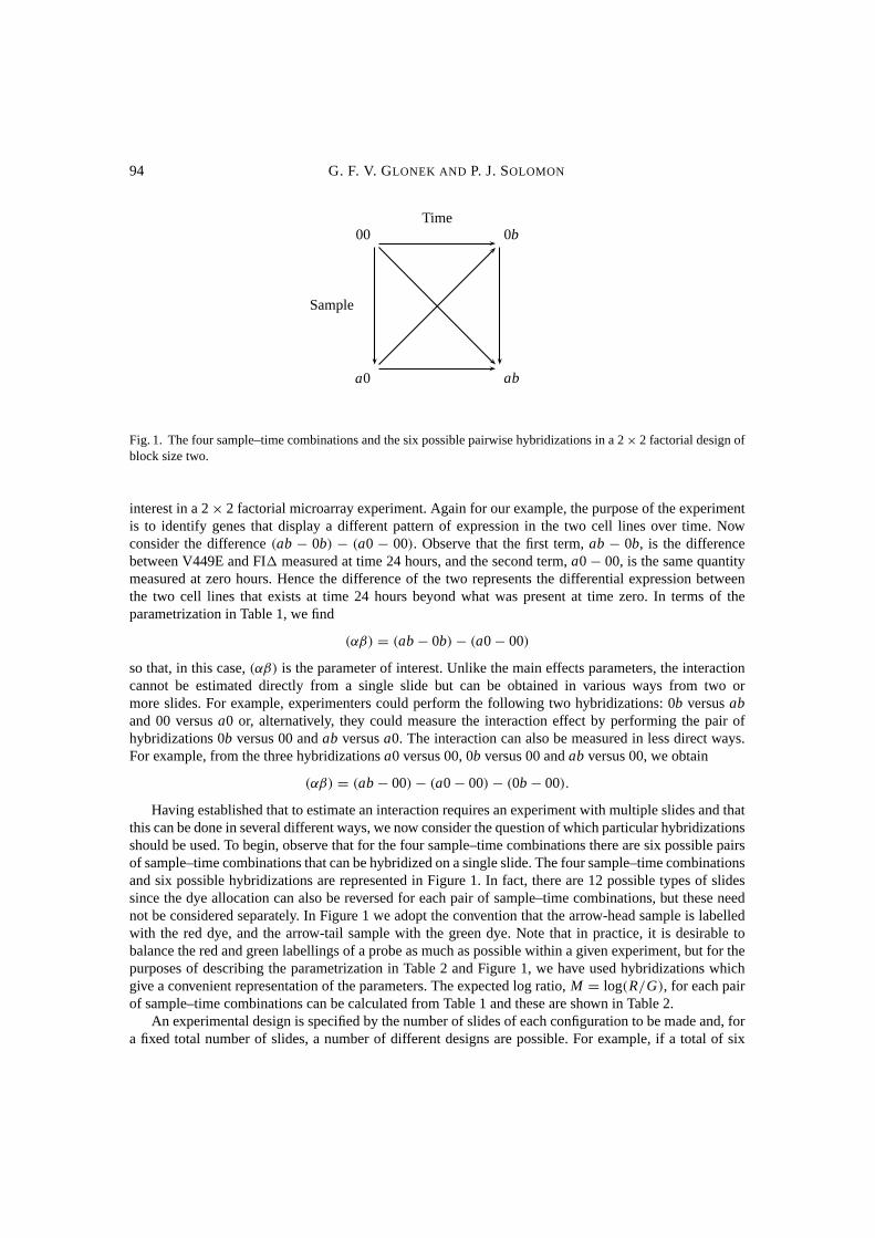
Fig. 1. The four sample–time combinations and the six possible pairwise hybridizations in a 2× 2 factorial design ofblock size two.
interest in a 2× 2 factorial microarray experiment. Again for our example, the purpose of the experimentis to identify genes that display a different pattern of expression in the two cell lines over time. Nowconsider the difference(ab − 0b) − (a0 − 00). Observe that the first term,ab − 0b, is the differencebetween V449E and FI� measured at time 24 hours, and the second term,a0 − 00, is the same quantitymeasured at zero hours. Hence the difference of the two represents the differential expression betweenthe two cell lines that exists at time 24 hours beyond what was present at time zero. In terms of theparametrization in Table 1, we find
(αβ) = (ab− 0b) − (a0 − 00)
so that, in this case,(αβ) is the parameter of interest. Unlike the main effects parameters, the interactioncannot be estimated directly from a single slide but can be obtained in various ways from two ormore slides. For example, experimenters could perform the following two hybridizations: 0b versusaband 00 versusa0 or, alternatively, they could measure the interaction effect by performing the pair ofhybridizations 0b versus 00 andab versusa0. The interaction can also be measured in less direct ways.For example, from the three hybridizationsa0 versus 00, 0b versus 00 andab versus 00, we obtain
(αβ) = (ab− 00) − (a0 − 00) − (0b − 00).
Having established that to estimate an interaction requires an experiment with multiple slides and thatthis can be done in several different ways, we now consider the question of which particular hybridizationsshould be used. To begin, observe that for the four sample–time combinations there are six possible pairsof sample–time combinations that can be hybridized on a single slide. The four sample–time combinationsand six possible hybridizations are represented in Figure 1. In fact, there are 12 possible types of slidessince the dye allocation can also be reversed for each pair of sample–time combinations, but these neednot be considered separately. In Figure 1 we adopt the convention that the arrow-head sample is labelledwith the red dye, and the arrow-tail sample with the green dye. Note that in practice, it is desirable tobalance the red and green labellings of a probe as much as possible within a given experiment, but for thepurposes of describing the parametrization in Table 2 and Figure 1, we have used hybridizations whichgive a convenient representation of the parameters. The expected log ratio,M = log(R/G), for each pairof sample–time combinations can be calculated from Table 1 and these are shown in Table 2.
An experimental design is specified by the number of slides of each configuration to be made and, fora fixed total number of slides, a number of different designs are possible. For example, if a total of six
Factorial and time course designs for cDNA microarray experiments 95
Table 2. Expected log ratioM = log(R/G)
Configuration ExpectedGreen Red log ratio
1 00 a0 α
2 00 0b β
3 00 ab α + β + (αβ)
4 0b ab α + (αβ)
5 a0 ab β + (αβ)
6 a0 0b β − α
µ
µ + α
µ + β
µ + α + β
2
13
Fig. 2. The usual reference design for six slides allocated as three dye-swapped pairs of hybridizations; thecombination with both factors at their lower level is the reference sample, represented by the parameterµ.
slides were available, a reference design comprising two replicates of each of configurations 1, 2 and 3of Table 2 could be used, as illustrated in Figure 2. The reference design allows for the estimation of allthree parameters of interest and has been used extensively in practice. An alternative design considered bySpeed (2001), is to use a single replicate of each of the six possible configurations as shown in Figure 1.As with the reference design, the all-pairwise comparison design allows for the estimation of the threeparameters of interest but it can be shown to have superior properties to the reference design. However,in the analyses that follow, we will demonstrate designs that are superior to both the reference and all-pairwise comparison designs. In particular, we show that despite its popularity and widespread acceptance,the reference design is very inefficient. We establish also that designs incorporating all possible directpairwise comparisons are rarely optimal by the criterion of statistical efficiency, regardless of whetherinterest centres on the main effects and interaction equally, or on the interaction effects alone; any benefitappears to lie solely in estimation of the main effects.
4.2 Statistical power and standard errors
The question of design can now be stated as: How many replicates of each configuration should beproduced? The standard way to answer this question would be to prescribe a suitable threshold valuefor M , say 4, and then require that the experiment have a pre-determined level ofpower, say 80%, againstany such alternatives. Such an experiment should then have an 80% chance of detecting any gene that is
96 G. F. V. GLONEK AND P. J. SOLOMON
log four fold over- or under-expressed. It is well known that such a requirement can be met by choosing adesign such that the standard error for each parameter of interest falls below a certain value. However, inpractice, the situation for microarrays is complicated. In particular, it can be shown that the standard errorof a given parameter estimate is given byσ
√c, whereσ is the standard deviation between slides for a
particular gene andc is a number derived from the design. However, a single experiment typically involvesanything between 10 000 and 20 000 genes in whichσ varies greatly from gene to gene, and is usuallyunknown. Therefore, the power typically cannot be determined in advance and, in a single experiment,we should not expect to attain the same level of power for every gene. Nevertheless, the design with thesmallest standard error and thus the highest power will be that which has the smallest value ofc and thisdoes apply equally to every gene.
4.3 Least squares estimates
A major step in the statistical analysis of a factorial microarray experiment is to obtain estimates of theparameters of interest and their standard errors. Both of these quantities can be obtained from the well-known theory of least squares estimation; see, for example, Searle (1971). For illustration, consider againthe 2× 2 factorial case and the reference design with two slides allocated to each of configurations 1, 2and 3 from Table 2. To calculate the least squares estimates, the design matrixX must be formed to reflectthe expected log intensity ratio for each slide, as specified in Table 2. In this case, the parameter vector istaken to beγ = (α, β, (αβ))T , so that the product
Xγ =
1 0 01 0 00 1 00 1 01 1 11 1 1
α
β
(αβ)
=
α
α
β
β
α + β + (αβ)
α + β + (αβ)
gives the expected log intensity ratios for the design. If the observed log intensity ratios are given bym = (m1, m2, m3, m4, m5, m6)
T , then the least squares estimates of the parameters are given in vectorform by (XT X)−1XT m, and the standard error of thei th parameter estimate is given byσ
√ci , whereci
is thei th diagonal element of the matrix(XT X)−1.
4.4 Admissible designs
It is reasonable, all other things being equal, that we should choose a design that makes each of theci
as small as possible. Unfortunately this criterion is not straightforward. If the total number of slides isfixed and a certain pair of designs is to be compared, it could be expected that some of theci will besmaller for the first design and some will be smaller for the second design. To illustrate, consider twoexperiments in the 2× 2 case, one comprising three replicates of each of the configurations 1, 2, 4 and5 from Table 2 and the other having four replicates of configurations 1, 2 and two of 4, 5. The designmatrices are, respectively,
X1 =1 1 1 0 0 0 1 1 1 0 0 0
0 0 0 1 1 1 0 0 0 0 0 00 0 0 0 0 0 1 1 1 1 1 1
T
and X2 =1 1 1 1 0 0 0 0 1 1 0 0
0 0 0 0 1 1 1 1 0 0 1 10 0 0 0 0 0 0 0 1 1 1 1
T
.
Factorial and time course designs for cDNA microarray experiments 97
The diagonal elements of(XT1 X1)
−1 are 1/4, 1/4 and 1/3 and the diagonal elements of(XT2 X2)
−1 are5/24, 5/24 and 3/8. Hence, for the same total number of slides, the first design provides slightly betterestimates for the interaction parameter(αβ) and the second provides slightly better estimates of the maineffectsα andβ.
On the other hand, it can happen that one design is better than another. For example, consider thereference design with four replicates of each of the configurations 1, 2, 3, so that the design matrix is
X3 =1 1 1 1 0 0 0 0 1 1 1 1
0 0 0 0 1 1 1 1 1 1 1 10 0 0 0 0 0 0 0 1 1 1 1
T
and the diagonal elements of(XT3 X3)
−1 are given by 1/4, 1/4 and 3/4. The conclusion is that the designX3 is inferior to bothX1 andX2 in terms of statistical efficiency. That is, for the same number of slides, thedesignX3 provides less accurate estimates ofall parameters. This is especially the case for the interactionparameter(αβ) which, as previously discussed, is often the parameter of primary importance. Theseconsiderations motivate the following definition.
DEFINITION 1 A design with a total ofn slides and design matrixX is said to beadmissibleif thereexists no other design withn slides and design matrixX∗ such that
ci � c∗i
for all i with strict inequality for at least one i, whereci , c∗i are respectively the diagonal elements of
(XT X)−1 and(XT∗ X∗)−1. A design that is not admissible is said to beinadmissible.
According to this definition, the designX3 is inadmissible sinceX1 and X2 are examples ofX∗ thatviolate the conditions for admissibility.
To illustrate the importance of choosing an efficient design, it is useful to compare the performance ofadmissible designs and some commonly used inadmissible alternatives. For simplicity we will considerthe 2× 2 factorial experiment with six slides. In this case there are 462 possible designs of which 21are admissible; these designs are shown in Table 3. Figure 3 presents diagrams of the three admissibledesigns which estimate the interaction parameter most efficiently. The design in the third row of Table 3corresponds to the third diagram in Figure 3 and Admissible Design 1 of Table 4, and is subject to theconstraint thatcα = cβ .
We now consider the performance of some inadmissible designs. To simplify the comparison, wecompare them only to the admissible designs which satisfy the additional constraintcα = cβ . Thereare three such designs and these are shown in Table 4. The first inadmissible design we consider is thereference design with two slides allocated to each of configurations 1, 2 and 3, as shown previously inFigure 2. Although this design has been widely used, the results of Table 4 show it to be very inefficientunder our formulation, especially with respect to the interaction parameter. Based on the comparison ofc(αβ), the Admissible Design 1 is clearly far superior to the reference design, and improves the efficiencyof estimation by 100%. In fact, it can be shown that the reference design would require 12 slides to achievethe same precision in estimating the crucial parameter(αβ).
The design considered recently by Speed (2001), comprising six slides corresponding to all sixpossible comparisons as shown in Figure 1, is also analysed in Table 4. Although superior to the referencedesign, it is nevertheless inadmissible and provides a substantially less precise estimate of(αβ) thanAdmissible Design 1, which here provides an efficiency gain of 33%. The reference design and the all-pairwise comparison design do provide for more efficient estimates of certain other contrasts, such asα − β andα + β + γ . However, a key element of our approach is to identify explicitly the contrasts that
Fig. 3. Three optimal admissible designs for 2× 2 factorial experiments with six slides: the three designs correspondto those with the smallestc(αβ) for estimation of the interaction parameter as set out in Table 3. The third design issubject to the constraint that the main effectsc’s are equal, i.e.cα = cβ , and corresponds to Admissible Design 1 inTable 4.
are of interest and optimize with respect to those. We argue that improved estimation of other contrasts isan unwarranted diversion of experimental effort rather than a virtue.
These examples show that large gains in efficiency can be obtained by using admissible designs. Theimproved efficiency ultimately translates into an enhanced ability to detect differential expression for agiven amount of experimental effort. For this reason, it is recommended that only admissible designs be
Factorial and time course designs for cDNA microarray experiments 99
2
4
5
163
F
V
0 24
(a)
2
4
5
1
(b)
2
4
5
1
(c)
2
4
5
1
(d)
Fig. 4. Four designs for the study of mutant leukaemic mice in which cell lines FI� (F) and V449E (V) were comparedat times zero and 24 hours. Each arrow represents a hybridization, and cell line comparisons at zero and 24 hours werereplicated with the dye assignment reversed. Eight slides in total were available in this experiment: (a) the designthat was used; (b) an admissible design; (c) our recommended admissible design; (d) the design used but with bothdiagonal comparisons omitted.
considered.In a given problem, that is, a set of possible configurations and total number of slides, there is no simple
way to identify the set of admissible designs. It transpires that, even for relatively small experiments, thereare a very large number of designs to choose from. For example, if a total of 24 slides are available, thenthere are 118 755 possible ways to allocate them amongst the six slide types shown in Table 2. However,for relatively small problems they can be identified by simple enumeration of all possibilities. In theAppendix, admissible designs for the 2× 2 case are listed for experiments with up to 18 slides andsubject to the additional constraint thatcα = cβ . In situations where the total number of slides is the onlyconstraint, it is our recommendation that only admissible designs be used.
4.5 The leukaemic mice case study revisited
The study of leukaemic mice motivated our consideration of the design issues discussed in this paper, butthe experiment itself was conducted prior to our elucidation of these issues. At the time, the best designappeared to be the all-pairwise comparison design—this design provides a robust and comprehensivebasis for estimation and statistical inference. Using the eight slides available, the six possible pairwisehybridizations were conducted and the cell line (i.e. sample) comparisons at times zero and 24 hours werereplicated since they represented the direct comparisons of most biological interest. The two replicatedhybridizations were performed as dye-swapped replicates.
The (inadmissible) experimental design we actually employed is shown in Figure 4(a). For this design,it can be checked thatcα = 1/3, cβ = 5/12 andc(αβ) = 2/3. The fact that this design is inadmissibleis demonstrated by the design shown in Figure 4(b). For that design, we havecα = 0.29,cβ = 0.39 andc(αβ) = 0.54. However, since estimation of the interaction parameter(αβ) is of primary interest, and forreasons of balance, we would recommend in practice that the admissible design shown in Figure 4(c) beused. For that design, we havecα = cβ = 3/8 andc(αβ) = 1/2. The simplest case of the 2× 2 factorialexperiment with eight slides corresponds to the ‘loop’ design advocated by Kerr and Churchill (2001).
It is of interest to observe that the diagonal comparisons used in the (inadmissible) case study design
100 G. F. V. GLONEK AND P. J. SOLOMON
Table 5.Two designs with six slides derived from theleukaemic mice experiment
do not contribute to the estimation of the interaction parameter. In particular, the design matrix is given by
X =1 −1 0 1 1 −1 0 1
0 0 1 1 0 0 1 10 0 0 1 1 −1 1 0
T
where the second and sixth rows ofX represent the dye-swapped replicates of configurations 1 and 4.The coefficients for estimation of the interaction(αβ) are given by the third row of(XT X)−1XT and arein this case1
3(−1, 1, −1, 0, 1, −1, 1, 0). This shows that(αβ) could have been estimated with the sameprecision if the experiment had used only the six slides of configurations 1, 2, 4 and 5, as shown in Figure4(d). In other words, two out of the eight slides do not contribute to the estimation of the key parameterof interest.
It is important to demonstrate that the differences in efficiency shown theoretically for different designsis observable in experimental data. A complete comparison of the data from the original eight-slideleukaemic mice experiment to the reduced version with six slides would need to take account of thecorresponding reduction in degrees of freedom. To avoid this complication, we compared the data obtainedfrom two six-slide experiments. In particular, we compared the six-slide experiment shown in Figure 4(d)to the all-pairs design obtained by removing one slide from of each of the dye-swapped replicate pairs. Inwhat follows, we refer to the two designs as A and B respectively. Table 5 shows the calculated variancesfor designs A and B. We observe that design A is admissible but, as shown previously, design B is not.
To demonstrate the apparent improvement likely to be realized in practice, the data corresponding todesigns A and B were analysed as separate experiments and the variance estimates for(̂αβ) calculated.Each slide consists of 16 128 spots so that there are 16 128 pairs of variances to be compared. The meanof these variances was 0.068 for design A and 0.088 for design B. There is also considerable variabilityfrom gene to gene arising from the variability in the mean squared error, and this is shown in Figure 5.The black points correspond to genes where the variance estimate from design A was lower and the greypoints are those for which design B was lower. We see that there is a modest but nevertheless clearlydiscernible benefit associated with the use of admissible design A. We would expect that a comparisonwith the reference design shown in Figure 2 would demonstrate an even more marked effect. It should benoted that the high degree of variability apparent in Figure 5 is due to the very small residual degrees offreedom for these designs and this aspect of the problem is quite separate from the issues considered inthis paper. From the perspective of designing an experiment, subject to a constraint on the total number ofslides, the most relevant comparison is that given in Table 5.
5. ADDITIONAL CONSTRAINTS
In practice, it sometimes happens that in addition to constraints on the total number of slides available,the amount of mRNA from the different sources is also limited. In this situation, the principle of selecting
Factorial and time course designs for cDNA microarray experiments 101
1 e05 1 e03 1 e01
1 e
051
e03
1 e
01
Design A
Des
ign
B
Fig. 5. Variance estimates for̂(αβ) from admissible design A and the all-pairs comparison design B, both with sixslides, for the leukaemic mice experiment.
admissible designs can still be applied. The only practical consideration is that the search must beconstrained to those designs compatible with the limitations on the available mRNA.
Consider the 2× 2 factorial design with a total of 18 slides available. With no constraints on theavailable mRNA, there are a total of 33 649 possible designs; the 16 admissible designs withcα = cβ
are shown in Table 17 in the Appendix. For illustration, suppose that for each of the combinationsa0,0b andab, there is only sufficient mRNA to producem slides, but that there is no limit on the baselinecombination 00. Ifm = 6, there is only one possible design with 18 slides, namely the reference designwith six replicates of each of the configurations 1, 2 and 3. At the other extreme, ifm = 18, then thereare no restrictions and the number of possible designs is 33 649. Table 6 shows the admissible designswith cα = cβ for m = 6, 7, 8 and 9. Whenm = 9, the number of possible designs is restricted to 2002and the design comprising five replicates of configurations 1 and 2 and four replicates of configurations4 and 5 appears as an admissible design within this restricted subset. It is of interest to observe that thesame design is also admissible when no restrictions are imposed, and produces the lowest possible valuefor c(αβ).
Another situation in which constraints may arise is in enabling comparability for multiple experiments.Suppose a certain treatment combination is likely to be used as the baseline treatment in several differentexperiments. We may then require that each treatment combination be hybridized with the baseline aprescribed minimum number of times. For example, consider again the 2× 2 factorial experiment with atotal of 18 slides and suppose that each of the combinationsa0, 0b andab are to be hybridized with thebaseline 00 at least twice. Our approach is then to consider admissible designs from within the constrainedsubset which, in this example, comprises 6188 possible designs. There are eight admissible designs withcα = cβ , and these are shown in Table 7.
The admissible designs obtained without constraint (see Tables 13–17 in the Appendix) generallyinclude only a very small number of slides of the configurations 3 and 6. The designs that give theoverall minimum value forc(αβ) contain no slides of either configuration. When additional constraintsare introduced, similar patterns are observed. In particular, the numbers of slides of the configurations 3
102 G. F. V. GLONEK AND P. J. SOLOMON
Table 6.Designs with 18 slides when available mRNA is restricted to m slides for each of a0,0b and ab
and 6 tend to be small and the designs which minimizec(αβ) prescribe the smallest possible numbersfor both configurations. It is interesting to observe that, excluding the trivial case where it was the onlypossible design, the reference design was not admissible in any context.
6. FACTORIAL EXPERIMENTS WITH MORE THAN TWO FACTORS OR TWO LEVELS
Our approach to the design of factorial microarray experiments can be used for experiments with morethan two factors and/or more than two levels per factor, and we now demonstrate the utility of admissibledesigns on a 2× 3 factorial experiment.
Illustration: a 2 × 3 experiment of GM-CSF. We are collaborating with researchers from the Instituteof Medical and Veterinary Science, Adelaide, on investigating the role of the cell-surface receptors fora group of signalling molecules in human disease. The signalling molecules are the cytokines GM-CSF,interleukin 5 and interleukin 3. The aim is to understand how these receptors are activated normally andwhat goes wrong with them in diseases such as leukaemia, certain solid cancers, asthma and rheumatoidarthritis. The experiment involves knocking out the GM-CSF receptor in a cell line and comparing it to theparental ‘normal’ cells. Two cell lines are compared in this experiment, mutant (M) and normal wild-type(W), at three time points: zero, six and 12 hours. The biologists are particularly interested in the cell line
Factorial and time course designs for cDNA microarray experiments 103
µ + γ
µ
µ + γ + α + αγ
µ + α
µ + γ + β + βγ
µ + β
0h 6h 12h
M
W
Fig. 6. Possible hybridizations for a 2×3 factorial experiment. The interaction parameters(αγ ) and(βγ ) are of mostinterest in this experiment, representing the changes in gene expression at six and 12 hours respectively.
comparisons at six and 12 hours. In what follows, we will suppose that 10 slides are available for theexperiment and that there are no other restrictions.
We decided in advance to consider only hybridizations for which the samples differ on one factor.That is, we consider comparisons of the two cell lines at the same time or comparisons of the samecell line at two different times, but exclude the case of comparing the two different cell lines at twodifferent times. The nine hybridizations we consider are shown in Figure 6. The parameterµ representsthe baseline (wild-type W at time zero),γ is the cell line (sample) parameter at time zero,α the differencein W between zero and six hours, andβ the change in W from six to 12 hours. The parameters of primaryinterest in this experiment are(αγ ) and(βγ ), the changes in expression between the cell lines at six hourscompared to time zero, and 12 hours compared to time zero, respectively. The main effect parametersα,β andγ are of secondary but nevertheless significant interest. Thea priori exclusion of the other sixcomparisons was largely for practical reasons. However, in the light of our experience with the 2× 2case, we considered it very unlikely that any such slides would feature in an optimal design. To choosean optimal design, all possible designs using 10 slides were enumerated and, subject to the constraintc(αγ ) = c(βγ ), 55 admissible designs were found. Of these, the design shown in Figure 7 provides thesmallest smallest value forc(αγ ). In particular, for this design we havecα = cβ = 0.66, cγ = 0.36 andc(αγ ) = c(βγ ) = 0.63.
7. TIME COURSE EXPERIMENTS
7.1 Parametrizations for time course experiments
The approach illustrated for factorial designs may also be applied in other situations such as time courseexperiments. Consider a simple time course experiment in which a single sample is to be analysed at times0, 1, 2, . . . , n, and for a single gene, letµt denote the level of expression at timet . A key step is to firstidentify the effects of interest. In contrast to the 2× 2 factorial experiment, where it is frequently the casethat the interaction parameter is unambiguously of prime importance, the situation for a time course willdepend more specifically on the particular context. In what follows, we will consider three approachesthat may be applicable in certain practical situations.
In the first, we assume that time zero represents a meaningful baseline and that the purpose is simply todetect differential expression relative to this baseline at any time. In this case, it would appear reasonableto define the parameters to beαt = µt − µ0 for t = 1, 2, . . . , n. The second situation we consider is
104 G. F. V. GLONEK AND P. J. SOLOMON
0h 6h 12h
M
W
Fig. 7. Best admissible design for a 2× 3 factorial experiment with 10 slides when interest is in the interactionparameters(αγ ) and(βγ ).
to define the parameters of interest as the differences between adjacent time points,δt = µt − µt−1 fort = 1, 2, . . . , r . This approach is relevant when the time scale is such that changes in expression are likelyto be observed as an abrupt step from one time point to the next and the purpose of the experiment is toidentify, for each gene, the time points at which such changes occur.
The third situation relevant to time course experiments and where our methods can be applied is whencertain time-profiles are specified in advance as being of interest. Supposer < n particular profiles aredefined in advance to be of interest. Then-dimensional space of all possible time profiles can then beparametrized by constructing a basis comprising ther profiles (vectors) of interest and anothern − rvectors that span the complementary space. The concept of admissibility can then be applied to identifythose designs that provide for the most efficient estimation of the coefficients associated with the profilesof interest. Suppose, for example, four equally-spaced time points are taken and let the space of all four-dimensional profiles,M = {(µ1, µ2, µ3, µ4)}, be parametrized in terms of orthogonal polynomials. Thefour basis vectors are
v0 =
0.50.50.50.5
, v1 =
−0.6708−0.22360.22360.6708
, v2 =
0.5−0.5−0.50.5
andv3 =
−0.22360.6708
−0.67080.2236
.
For the purposes of illustration, we will consider designs that are optimal for the estimation of thelinear and quadratic terms. The same approach can also be used for any other specified profiles of interest.However, it would seem that the designs tailored for the estimation of the linear and quadratic terms wouldalso be well suited to the estimation of any other profile that is well approximated by a quadratic functionof time.
7.2 Designs
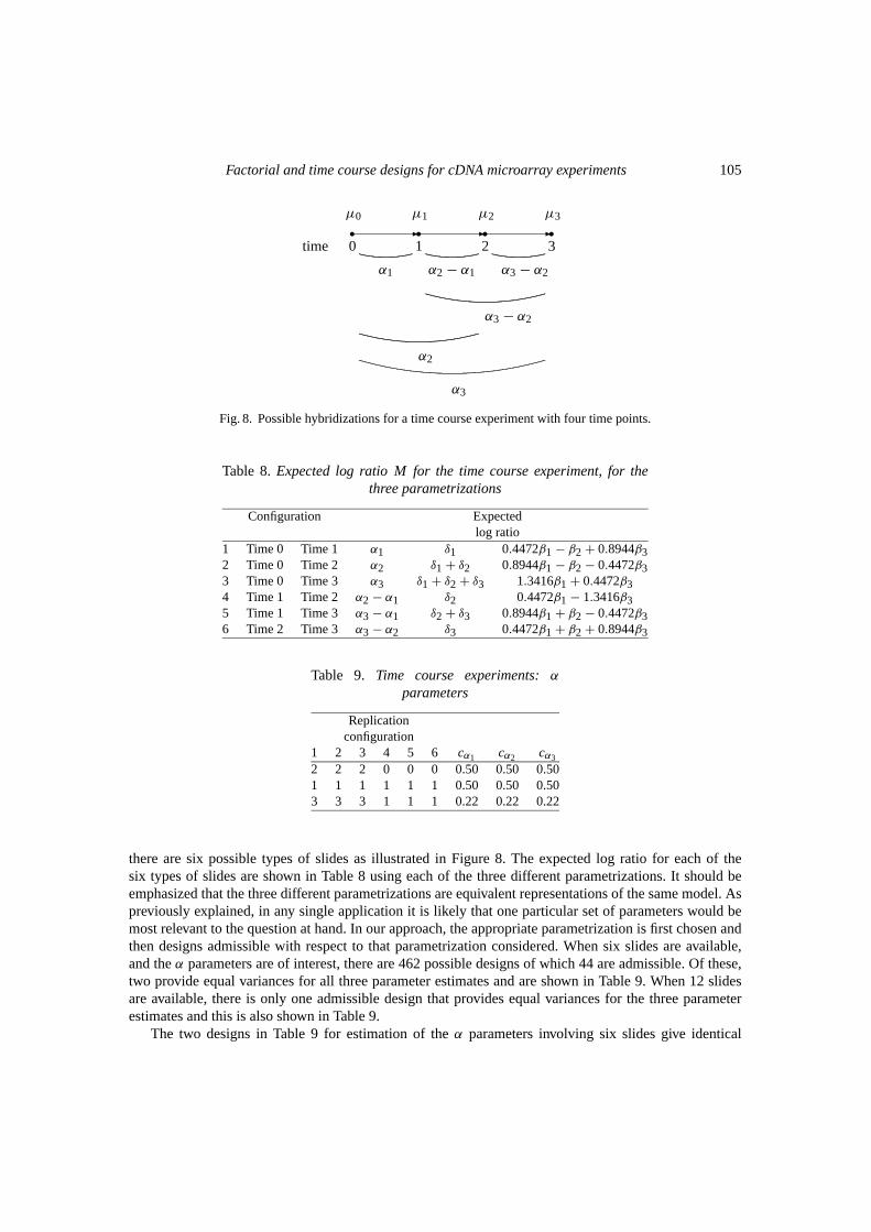
To demonstrate the application of our methods, the admissible designs are calculated under each of thethree situations discussed above for time course experiments with four time points and six or 12 slides.In a time course experiment withn time points, there aren(n + 1)/2 possible slides and the questionof design again amounts to that of how many slides of each type should be made. In the casen = 4,
Factorial and time course designs for cDNA microarray experiments 105
µ0 µ1 µ2 µ3�� �� �� �
time 0 1 2 3
α1 α2 − α1 α3 − α2
α3 − α2
α2
α3
Fig. 8. Possible hybridizations for a time course experiment with four time points.
Table 8.Expected log ratio M for the time course experiment, for thethree parametrizations
Configuration Expectedlog ratio
1 Time 0 Time 1 α1 δ1 0.4472β1 − β2 + 0.8944β32 Time 0 Time 2 α2 δ1 + δ2 0.8944β1 − β2 − 0.4472β33 Time 0 Time 3 α3 δ1 + δ2 + δ3 1.3416β1 + 0.4472β34 Time 1 Time 2 α2 − α1 δ2 0.4472β1 − 1.3416β35 Time 1 Time 3 α3 − α1 δ2 + δ3 0.8944β1 + β2 − 0.4472β36 Time 2 Time 3 α3 − α2 δ3 0.4472β1 + β2 + 0.8944β3
there are six possible types of slides as illustrated in Figure 8. The expected log ratio for each of thesix types of slides are shown in Table 8 using each of the three different parametrizations. It should beemphasized that the three different parametrizations are equivalent representations of the same model. Aspreviously explained, in any single application it is likely that one particular set of parameters would bemost relevant to the question at hand. In our approach, the appropriate parametrization is first chosen andthen designs admissible with respect to that parametrization considered. When six slides are available,and theα parameters are of interest, there are 462 possible designs of which 44 are admissible. Of these,two provide equal variances for all three parameter estimates and are shown in Table 9. When 12 slidesare available, there is only one admissible design that provides equal variances for the three parameterestimates and this is also shown in Table 9.
The two designs in Table 9 for estimation of theα parameters involving six slides give identical
variances for the parameter estimates and it is therefore of interest to compare the covariance matrices.These are given respectively by
0.5 0 0
0 0.5 00 0 0.5
and
0.5 0.25 0.25
0.25 0.5 0.250.25 0.25 0.5
.
The positive covariances in the second design indicate, as would be expected, that the second designprovides superior estimates of differencesαt1 − αt2.
When six slides are available, and theδ parameters are of interest, there are 462 possible designs ofwhich 36 are admissible. Of these, two provide equal variances for all three parameter estimates and areshown in Table 10. However, if a total of 12 slides are available, it transpires that of the 352 admissibledesigns, none provide equal variance for each of the three parameter estimates. An obvious choice forthe design with 12 slides might then be to simply double the numbers of slides from the two admissibledesigns for the six slides. Clearly both of those designs will givecδ1 = cδ2 = cδ3 = 0.25. In this case,there are seven admissible designs that provide lower variances for all three parameter estimates and theseare listed in Table 11.
Finally, we consider admissible designs for the parametrization based on the orthogonal polynomials.When six slides are available, there are 462 possible designs of which 71 are admissible. Of these, oneprovides equal variances for the parameter estimatesβ̂1 andβ̂2 and these are shown in Table 12. Similarly,when 12 slides are available, there are two admissible designs that provide equal variances and these arealso given in Table 12.
In the light of these considerations, designs that allocate equal numbers of each of the six possibletypes of slides would seem to be well suited to the time course experiment with four time points. Althoughthey are not necessarily optimal, the preceding calculations show that they are quite efficient in all threesituations. Moreover, the balance in these designs is an attractive property that may well out-weigh theminor losses in efficiency.
Factorial and time course designs for cDNA microarray experiments 107
One of the key steps in the development of this paper is the identification of the parameters of interest.Although this may be an unfamiliar step for many experimentalists, it is necessary for any formulationof good design and in many contexts should be straightforward. It is important to note that, for a givenset of possible hybridizations, the corresponding levels of expression can be described using appropriateparameters in several different, but equivalent, ways. See, for example, Tables 9 and 10 in the contextof the time course experiment. Moreover, the experimental designs that are optimal for one particularparametrization may not be optimal for a different parametrization of the same experiment. The keypoint to be made here is that the parameters must be formulated to correspond directly to the underlyingquestions of substantive interest. In non-technical terms, this amounts to the fact that experiments can bedesigned to answer specific questions in a given context. One should not expect an experiment designedfor a particular question to be optimal for answering some other question. Further issues arise whenparameters of subsidiary interest, such as main effect parameters, are present or when a question involvingseveral parameters simultaneously is of interest. The treatment of those issues is somewhat technical andbeyond the scope of the present paper.
8.2 Additional contrasts
In this paper, we began with the parametrization given in Table 1 and then studied the question of howbest to design an experiment to estimate efficiently the parameters of interest. In the 2× 2 experiment, itis frequently the case that the interaction parameter is the sole parameter of interest. However, in differentexperiments it may happen that both the original parameters and some additional derived contrasts are ofequal interest. For example, in the simple time course experiment, it may be of equal interest to estimateboth theα andδ parameters. In algebraic terms, this leads to a certain redundancy in the sense that if weknow the values of theα parameters we can use that information to deduce the values of theδ parameters.As was previously discussed, it is not the case that the designs which give the best estimate of theα
parameters are also optimal for estimatingδ. In this case, the definition of admissibility could be extendedto find designs that best accommodate both requirements. This extension will be the subject of future work.
8.3 Larger scale studies
The examples considered in this paper have been small in terms of both the number of parametersinvolved and the number of slides available. In situations involving a larger number of parameters, thesame arguments for considering only admissible designs can be made. However, in such cases it mayhappen that the number of admissible designs is so large that it is not useful simply to examine the list.In such cases, additional criteria for selecting a design are needed. If the number of parameters is small
108 G. F. V. GLONEK AND P. J. SOLOMON
but a large number of slides are available, then a different problem arises. Namely, the total number ofconfigurations rapidly becomes too large for the enumeration methods used here to be feasible. Althoughthe problems outlined above are yet to be resolved, it has been our experience that our methods are usefulfor many experiments currently being considered in practice.
8.4 Robustness
In this paper, we have been primarily concerned with finding admissible designs subject to a singleconstraint on the total number of slides. In Section 5, we considered further contraints owing to limitationson the available mRNA. In practice, it may be necessary to introduce constraints for other reasons. Forexample, we might require a design with even numbers of each type of slide so that dye-swapping can beused or, more importantly, the requirement may be for a design in which all parameters can be estimatedeven if one slide fails completely. The latter is only likely to be a problem in small experiments with a verysmall number of replicated slides, but it raises the general issue of robustness of admissible designs. Oneapproach would be to consider only designs with the property that all parameters remain estimable whenany single slide is removed, and then choose a design admissible within the restricted subset. However,most of the admissible designs in Tables 13–17 already have this property so, in practice, it would appearthat conducting a restricted search to identify robust, admissible designs may not be necessary.
8.5 Classical designs
In this paper, we have described in detail simple notional applications of factorial and time course designsto microarray experiments. It is important to recognize that classical designs and standard approachesto estimation seek to minimize the standard error of all estimable treatment contrasts, whereas we areinterested in particular contrasts, frequently although not exclusively the interaction parameter. Moreover,owing to the practical constraints often arising in microarray experimentation due to limited numbers ofslides, limitations on the available mRNA probes, uncertainty about the actual experimental process, andso on, each complex experiment needs its own tailor-made design. In other words, although it is possible togenerate banks of admissible designs, it is very useful to have a way of treating each experiment on a case-by-case basis to accommodate features particular to that experiment. Furthermore, classical experimentaldesign does not offer optimal designs of direct practical utility to the microarray context, and althoughthere is a large and established literature on classical experimental design, it has not been able to offerdefinitive answers for even the simplest microarray experiments.
In summary, we have proposed classes ofadmissible designs, for factorial and time course microarrayexperiments with a fixed number of arrays available for experimentation and information on the effects ofprimary interest to biologists. For relatively small problems, this may be done simply by enumerating thepossibilities. For larger problems, where the number of possible configurations is so large that enumerationis not feasible, we are presently exploring approximate methods of optimisation. The anticipated result ofthis research will be a computational tool that enables experimentalists and other researchers to identifygood designs in problems too large to be analysed by enumeration.
ACKNOWLEDGEMENTS
This work was supported in part by the Australian Research Council. We are grateful to TerrySpeed for advice and inspiration, and to Anna Tsykin for helpful discussions on the biological aspectsof microarray experiments. We acknowledge our biological collaborators Richard D’Andrea, BrentonReynolds, Tom Gonda, Mark Guthridge and Greg Goodall.
The calculations for this paper were performed using a computer program written in C++ by theauthors. A copy of the program will be provided on request.
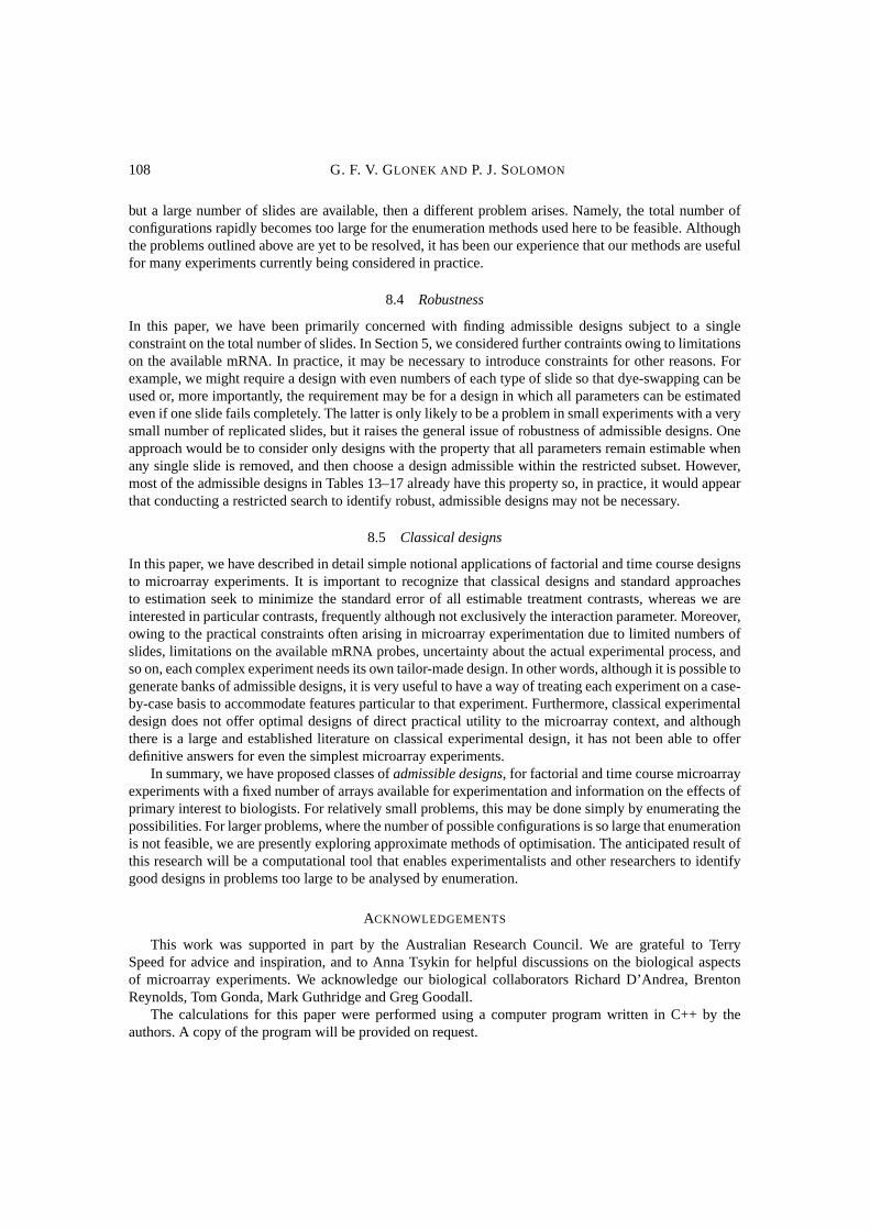
Factorial and time course designs for cDNA microarray experiments 109
In this section, we present the key admissible designs for 2× 2 factorial experiments on 8, 10, 12, 16and 18 slides. The results presented generalize those in Table 3 for six slides, but assume that the maineffects are to have equal variances. These tables were produced using a C++ program that identifies theadmissible designs in a given situation by enumeration. We offer these designs here in the hope that theymay be informative to researchers on the brink of conducting 2×2 factorial microarray experiments. Notethat it is not necessary to assume an even number of slides; we have done so for convenience and to enabledye-swapped replication when feasible. It is clear that the ‘cross-hybridizations’ rarely enter the optimaladmissible designs.
BROWN, P. AND BOTSTEIN, D. (1999). Exploring the new world of the genome with DNA microarrrays.NatureGenetics (Suppl.)21, 33–37.
CHURCHILL, G. A (2002). Fundamentals of experimental design for cDNA microarrays.Nature Genetics (Suppl.)32, 490–495.
DUDOIT, S., YANG, Y., CALLOW, M. AND SPEED, T. P. (2002). Statistical methods for identifying differen-tially expressed genes in replicated cDNA microarray experiments.Statistica Sinica12, 111–139.
EISEN, M. AND BROWN, P. O. (2000). DNA arrays for analysis of gene expression.Methods in Enzymology303,179–205.
JIN, W., RILEY , R., WOLFINGER, R., WHITE, K., PASSADOR-GURGEL, G. AND GIBSON, G. (2001). Thecontributions of sex, genotype and age to transcriptional variance inDrosophila melanogaster. Nature Genetics29, 389–395.
KERR, M. AND CHURCHILL, G. A. (2001). Experimental design for gene expression microarrays.Biostatistics2,183–201.
NGUYEN, D., ARPAT, A., WANG, N. AND CARROLL, R. (2002). DNA microarray experiments: biological andtechnical aspects.Biometrics58, 701–717.
PAN, W., LIN, J. AND LE, C. (2002). How many replicates of arrays are required to detect gene expression changesin microarray experiments? A mixture model approach.Genome Biology3, research0022.1–0022.10.
SCHENA, M. (2003).Microarray Analysis. Hoboken: Wiley.
Factorial and time course designs for cDNA microarray experiments 111
SEARLE, S. (1971).Linear Models. NewYork: Wiley.
SPEED, T. P. (2001).Gene Expression, Wald Lecture III, Joint Statistical Meetings, August 2001.http://www.
stats.berkeley.edu/users/terry
SPEED, T. P AND YANG, Y. H. (2002). Direct versus indirect hybridizations for cDNA microarrayexperiments.Sankhya A Series A64, 707–721.
WOLFINGER, R., GIBSON, G., WOLFINGER, E., BENNETT, L., HAMADEH , H., BUSHEL, P., AFSHARI, C. AND
PAULES, R. (2001). Assessing gene significance from cDNA microarray expression data via mixed models.Journal of Computational Biology8, 625–638.
YANG, Y. H., BUCKLEY, M., DUDOIT, S. AND SPEED, T. P. (2002a). Comparison of methods for image analysison cDNA micrarray data.Journal of Computational and Graphical Statistics11, 108–136.
YANG, Y., DUDOIT, S., LUU, P., LIN, D., PENG, V., NGAI, J. AND SPEED, T. P. (2002b). Normalization forcDNA microarray data: a robust composite method addressing single and multiple slide systematic variation.Nucleic Acids Research30, e15.
YANG, Y. H. AND SPEED, T. P. (2002). Design issues for cDNA microarray experiments.Nature Reviews Genetics3, 579–588.
YANG, Y. H. AND SPEED, T. P. (2003). Design and analysis of comparative microarray experiments. In Speed, T. P.(ed.),Statistical Analysis of Gene Expression Microarray Data, Boca Raton, FL: CRC Press.
[Received December, 9 2002; first revision April, 2 2003; second revision June, 29 2003;accepted for publication August, 7 2003]


![[Simmons G.F.] Introduction to Topology and Modern](https://static.documents.pub/doc/80x56/544f519eb1af9fff3e8b4b5e/simmons-gf-introduction-to-topology-and-modern.jpg)


