The User’s Guide, as well as the software described in it, is furnished under license and may only be used or copied in accordance withthe terms of such license. The information in this User’s Guide is furnished for informational use only, is subject to change withoutnotice, and should not be construed as a commitment by Northwest Geophysical Associates, Inc. Northwest Geophysical Associatesassumes no responsibility or liability for any errors or inaccuracies that may appear in this booklet.
GM-SYS is a registered trademark of Northwest Geophysical Associates, Inc.
Adobe, Acrobat, PostScript, and Adobe Illustrator are trademarks of Adobe Systems Incorporated which may be registered incertain jurisdictions.
AutoCAD is a registered trademark of Autodesk, Inc.CorelDraw is a registered trademark of Corel Corporation.GeoGraphix is a registered trademark of Landmark Company.GeoSec and GeoSec2D are trademarks or registered trademarks of Paradigm Geophysical Ltd.Geosoft and OASIS montaj are registered trademarks or trademarks of Geosoft, Inc.Sentinel SuperPro is a trademark of Rainbow Technologies.Windows, Windows NT, Microsoft and MS-DOS are either registered trademarks or trademarks of Microsoft Corporation in the
United States and/or other countries.2MOD is a registered trademark of Fugro-LCT, Inc.
Included Software
ImageMagick is Copyright 2000 ImageMagick Studio, a non-profit organization dedicated to making software imaging solutionsfreely available.
Permission is hereby granted, free of charge, to any person obtaining a copy of this software and associateddocumentation files ("ImageMagick"), to deal in ImageMagick without restriction, including without limitation the rights touse, copy, modify, merge, publish, distribute, sublicense, and/or sell copies of ImageMagick, and to permit persons towhom the ImageMagick is furnished to do so, subject to the following conditions:
The above copyright notice and this permission notice shall be included in all copies or substantial portions ofImageMagick.
The software is provided "as is", without warranty of any kind, express or implied, including but not limited to thewarranties of merchantability, fitness for a particular purpose and noninfringement. In no event shall ImageMagick Studiobe liable for any claim, damages or other liability, whether in an action of contract, tort or otherwise, arising from, out of orin connection with ImageMagick or the use or other dealings in ImageMagick.
Except as contained in this notice, the name of the ImageMagick Studio shall not be used in advertising orotherwise to promote the sale, use or other dealings in ImageMagick without prior written authorization from theImageMagick Studio.
2.3 Creating a New Model ............................................................................ 162.3.1 Overview of New Model Creation ................................................... 162.3.2 Cross-Section Limits ....................................................................... 162.3.3 Profile Azimuth/Relative Strike Angle .............................................. 172.3.4 Topography and Gravity & Magnetics Stations ............................... 172.3.5 Choosing the Gravity Anomaly to Model: Free-Air, Residual, orBouguer ................................................................................................... 172.3.6 Earth's Magnetic Field .................................................................... 18
2.4 Importing a Model from Another Modeling Application ............................ 182.5 Menu Overview ....................................................................................... 18
File Menu ................................................................................................. 18View Menu ............................................................................................... 18Overlay Menu .......................................................................................... 18Display Menu ........................................................................................... 18Profile Menu ............................................................................................ 19Gradients Menu ....................................................................................... 19Action Menu............................................................................................. 19Compute Menu ........................................................................................ 19
Table of Contents4
GM-SYS® v. 4.9
Window Menu .......................................................................................... 19Help Menu ............................................................................................... 19
3. MODELING CONCEPTS ....................................................................... 213.1 Uniqueness ............................................................................................. 213.2 DC Shift ................................................................................................... 213.3 2-D Modeling........................................................................................... 213.4 2¾-D Modeling ........................................................................................ 223.5 Skewed Models ....................................................................................... 223.6 Inversion ................................................................................................. 233.7 Computational Basis for GM-SYS ........................................................... 233.8 Single Block Response ........................................................................... 243.9 Rotated-to-Pole & ROTATED-TO-equator Magnetic Data ...................... 243.10 Choice of Gravity Anomaly: Free-Air, Residual, or Bouguer ................. 243.11 Magnetic Units....................................................................................... 243.12 Gravity Units ......................................................................................... 273.13 Gravity & Magnetic Gradients ............................................................... 27
3.13.1 Gradient Axis ................................................................................ 293.13.2 Magnetic Gradient Display and Units............................................ 293.13.3 Gravity Gradients Display and Units ............................................. 29
3.14 Grid Output ........................................................................................... 293.15 Symbol Display ..................................................................................... 303.16 Well Display ....................................................................................... 303.17 Bitmap Display ...................................................................................... 30
4. MODEL ELEMENTS ............................................................................ 334.1 Surfaces .................................................................................................. 334.2 Points ...................................................................................................... 334.3 Blocks ..................................................................................................... 33
4.3.1 Block Labels ................................................................................... 344.3.2 Block Data ...................................................................................... 34
4.4 Backdrop Images .................................................................................... 344.5 Symbols .................................................................................................. 354.6 Well Markers and LAS well files .............................................................. 354.7 Gravity and Magnetic Stations ................................................................ 35
5.1.1 File Menu ........................................................................................ 38New Model and Open Model .............................................................. 38
Table of Contents 5
GM-SYS® v. 4.9
Save Model and Save as ................................................................... 38Close .................................................................................................. 38Preferences ........................................................................................ 38Print .................................................................................................... 39Exit ..................................................................................................... 39Previously Opened Model List ............................................................ 39
5.1.2 View Menu ...................................................................................... 39Previous View .................................................................................... 39Mark Current View.............................................................................. 40Add Current View ............................................................................... 40Edit Views .......................................................................................... 40View List ............................................................................................. 40
5.1.3 Overlay Menu ................................................................................. 41Backdrop ............................................................................................ 41Symbols ............................................................................................. 42Edit Wells ........................................................................................... 42LAS Wells ........................................................................................... 43Block Fill ............................................................................................. 43
5.1.4 Display Menu .................................................................................. 445.1.5 Profile Menu ................................................................................... 44
Set Mag. Field .................................................................................... 44Set Azi./Strike Angle ........................................................................... 45Set Real-World Origin Coord. ............................................................. 45Set Plan View Depth .......................................................................... 45Edit Anomaly ...................................................................................... 45Edit Wells ........................................................................................... 45Edit Blocks ......................................................................................... 45Magnetics Elevation Adjust ................................................................ 46Magnetics DC Shift ............................................................................ 46Gravity Elevation Adjust & Gravity DC Shift ....................................... 46
5.1.7 Action Menu .................................................................................... 47Undo................................................................................................... 47
Table of Contents6
GM-SYS® v. 4.9
Move Point ......................................................................................... 47Move Group ....................................................................................... 48Add Point ............................................................................................ 48Delete Point ........................................................................................ 48Split Block........................................................................................... 48Delete Surface ................................................................................... 48Examine ............................................................................................. 48Box Zoom ........................................................................................... 492X Zoom In......................................................................................... 492X Zoom Out ...................................................................................... 49Invert .................................................................................................. 49Move Label ......................................................................................... 51
5.1.8 Compute Menu ............................................................................... 515.1.9 Window Menu ................................................................................. 515.1.10 Help Menu .................................................................................... 51
5.2 Menu Tool Bar ......................................................................................... 525.2.1 Cursor tracking ............................................................................... 525.2.2 Import/Export Horizon ..................................................................... 52
7.1 Surface (.SUR) File Format..................................................................... 627.2 Block (.BLK) File Format ......................................................................... 637.3 Gravity (.GRV) File Format ..................................................................... 647.4 Gravity Gradient (.GDO) File Format ...................................................... 647.5 Magnetics (.MAG) File Format ................................................................ 657.6 Magnetic Gradient (.MDO) File Format ................................................... 657.7 View (.VEW) File Format......................................................................... 667.8 Well (.WEL) File Format .......................................................................... 667.10 Extended Coordinate System (.ECS) File Format................................. 677.11 Generic Space-delimited ASCII ............................................................. 677.12 Symbol definition File ............................................................................ 677.13 Patterns................................................................................................. 68
8. CVTGMS ...................................................................................... 698.1 Getting Started ........................................................................................ 69
8.1.1 Modifying the model ....................................................................... 698.1.2 Output ............................................................................................. 70
8.2 Menus ..................................................................................................... 708.2.1 File Menu ........................................................................................ 70
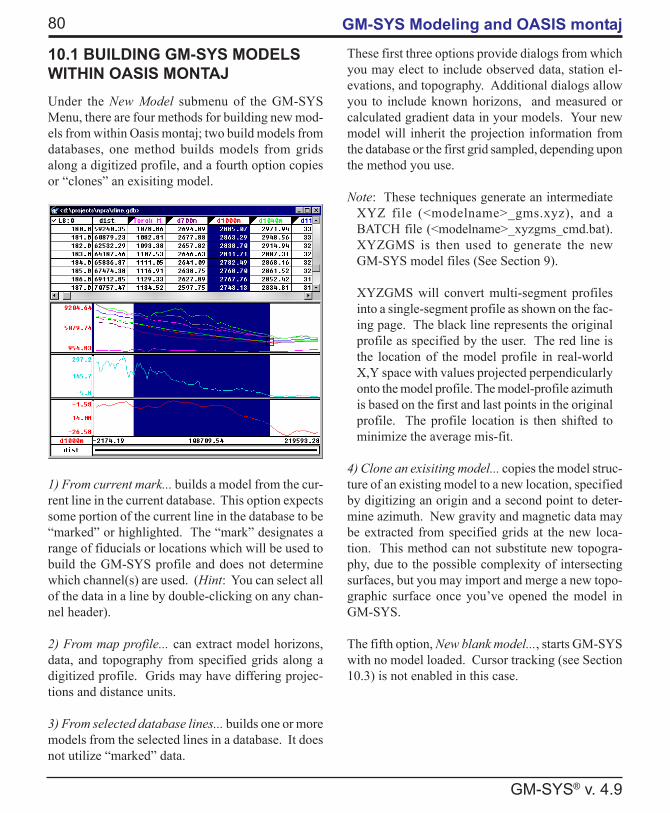
10. GM-SYS MODELING AND OASIS MONTAJ ....................................... 7910.1 BUILDING GM-SYS models within OASIS montaj................................ 8010.2 Working with existing models within OASIS montaj .............................. 8110.3 Cursor Tracking ..................................................................................... 8110.3 Loading GM-SYS plots into geosoft maps ............................................ 81
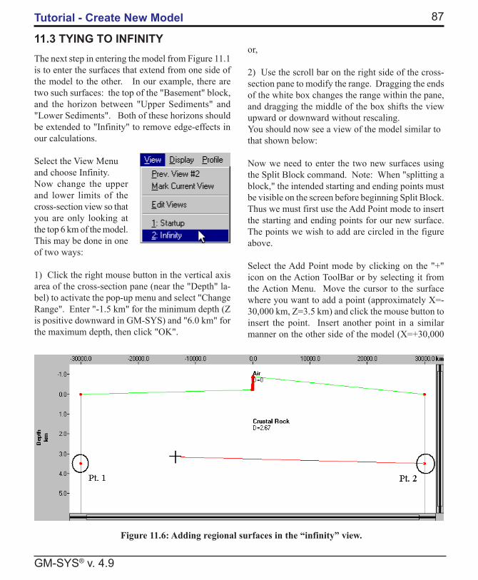
11. TUTORIAL - CREATE NEW MODEL ..................................................... 8311.1 Overview ............................................................................................... 8311.2 Create New Model................................................................................. 8411.3 Tying To Infinity ...................................................................................... 8711.4 Sketching Your Model............................................................................ 89
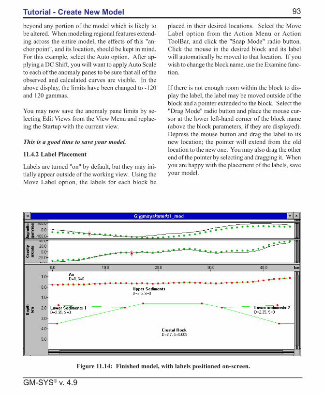
11.4.1 Applying a DC Shift ....................................................................... 9111.4.2 Label Placement ........................................................................... 93
SOFTWARE LICENSE AGREEMENTThis is a legal agreement between you (either an individual or an entity) and Northwest Geophysical Associ-ates, Inc. (NGA). By using this software, you agree to become bound by the terms of this agreement. Theterm “SOFTWARE” also shall include any upgrades, modified versions or updates of the software licensed toyou by NGA. The SOFTWARE that accompanies this license is the property of NGA and its Licensors and isprotected by copyright law. If you do not agree to the terms of this Agreement, do not use the software.Promptly return the entire package to NGA or the distributor where you obtained it for a full refund.
1. GRANT OF LICENSE. NGA and its Licensors, grant to you, the Licensee, the nonexclusive right to usethis SOFTWARE as defined by this agreement. The term of the license is indefinite unless there is a breach ofthe license agreement. Upon termination, the purchaser returns all copies of the SOFTWARE and documen-tation together with a signed affidavit to the effect that all copies have been returned. Licensee is grantedpermission to print, as necessary, the electronic User’s Guide for Licensee use only.
2. SCOPE OF LICENSE. If you acquired a Single-User License, you may install the SOFTWARE ondifferent computers at your physical address and you must have a mechanism or process in place to assure thatonly one copy of the program is in use at any time for each license. If you acquired a “SITE LICENSE” youare granted the right to use the SOFTWARE simultaneously on the number of computers granted by the SITELICENSE at your physical address.
3. OWNERSHIP OF SOFTWARE. NGA and its Licensors retain the copyright, trademarks, titles, andownership of the SOFTWARE and the related written materials regardless of the form or media on which theoriginal and other copies may exist. The Licensee may make one (1) copy of the SOFTWARE solely forbackup purposes. You must reproduce and include the copyright notice on the backup copy. You may notreverse engineer, decompile, or disassemble the SOFTWARE. This Agreement does not grant you any intel-lectual property rights in the SOFTWARE.
4. SUPPORT. Licenses include service contract support and updates for six months from original purchasedate. Support includes phone assistance, prompt correction of reported errors, manual revisions, and periodicSOFTWARE updates. Support is available after the initial six month period for a fee and includes any productupdates during that support period.
5. TRANSFERS. You may transfer the SOFTWARE from one computer to another at the Licensee physicaladdress provided that the SOFTWARE is used in accordance with Section 2, SCOPE OF LICENSE, aswritten above. Except within the bounds of this agreement, you may not distribute copies of the SOFTWAREor accompanying written materials to others. You may not transfer the SOFTWARE to a different physicaladdress or anyone else without the prior written consent of NGA. In no event may you transfer, assign, rent,lease, sell or otherwise dispose of the SOFTWARE on a temporary basis.
6. LIMITED WARRANTY. With respect to the distribution media and physical documentation enclosedherein, NGA warrants the same to be free of defects in materials and workmanship for a period of 60 daysfrom the date of purchase. In the event of notification within the warranty period of defects in material orworkmanship, NGA will replace the defective distribution media or documentation. The remedy for breach ofthis warranty shall be limited to replacement and shall not encompass any other damages, including but notlimited to loss of profit, special, incidental, consequential, or other similar claims. NGA and its Licensors donot warrant that the SOFTWARE will meet your requirements or that operation of the SOFTWARE will beuninterrupted or that the SOFTWARE will be error-free.
Software License12
NGA AND ITS LICENSORS SPECIFICALLY DISCLAIM ALL OTHER WARRANTIES, EXPRESSEDOR IMPLIED, INCLUDING BUT NOT LIMITED TO, IMPLIED WARRANTIES OF MERCHANTABIL-ITY AND FITNESS FOR A PARTICULAR PURPOSE. IN NO EVENT SHALL NGA AND ITS LICEN-SORS BE LIABLE FOR ANY LOSS OF PROFIT OR ANY OTHER COMMERCIAL DAMAGE, INCLUD-ING BUT NOT LIMITED TO SPECIAL, INCIDENTAL, CONSEQUENTIAL OR OTHER DAMAGES.
7. GENERAL. The laws of the State of Oregon will govern this Agreement. This Agreement may only bemodified by a license addendum, which may accompany this license, or by a written document which hasbeen signed by both you and NGA. Should you have questions concerning this Agreement, or if you desire tocontact NGA for any reason, please write: NGA Client Sales and Service, P.O. Box 1063, Corvallis, OR97339-1063, USA.
13
GM-SYS® v. 4.9
Introduction
1. INTRODUCTION
GM-SYS is a program for calculating the gravity andmagnetic response from a geologic model. GM-SYSprovides an easy-to-use interface for interactivelycreating and manipulating models to fit observedgravity and/or magnetic data. Rapid calculation ofthe gravity and magnetic response from 2D and 2¾-Dmodels speed the interpretation process and allowsyou to quickly test alternative solutions.
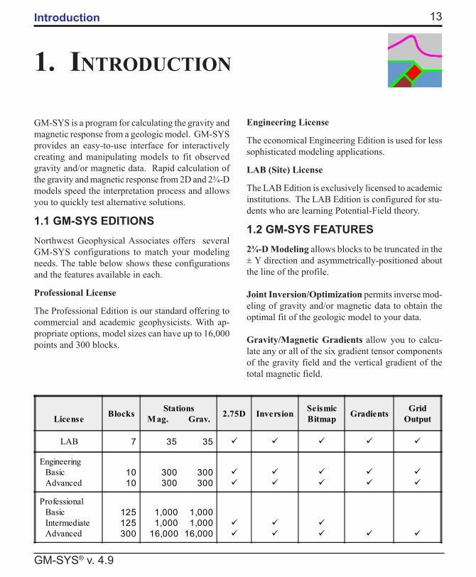
1.1 GM-SYS EDITIONSNorthwest Geophysical Associates offers severalGM-SYS configurations to match your modelingneeds. The table below shows these configurationsand the features available in each.
Professional License
The Professional Edition is our standard offering tocommercial and academic geophysicists. With ap-propriate options, model sizes can have up to 16,000points and 300 blocks.
Engineering License
The economical Engineering Edition is used for lesssophisticated modeling applications.
LAB (Site) License
The LAB Edition is exclusively licensed to academicinstitutions. The LAB Edition is configured for stu-dents who are learning Potential-Field theory.
1.2 GM-SYS FEATURES2¾-D Modeling allows blocks to be truncated in the± Y direction and asymmetrically-positioned aboutthe line of the profile.
Joint Inversion/Optimization permits inverse mod-eling of gravity and/or magnetic data to obtain theoptimal fit of the geologic model to your data.
Gravity/Magnetic Gradients allow you to calcu-late any or all of the six gradient tensor componentsof the gravity field and the vertical gradient of thetotal magnetic field.
IntroductionSeismic Bitmap permits integration of seismic dataor other depth-scaled information (e.g. scanned cross-sections) into the modeling process.
Grid Output allows you calculate the response of amodel as a Geosoft grid (.grd) file. You may elect tocalculate the response at a fixed elevation, or at aconstant terrain separation.
Extended Model Size increases maximum allowablemodel size to 750 surfaces and 300 blocks.
High Resolution Modeling increases the number ofallowable gravity and magnetic observation and cal-culation points to 16,000.
Oasis montaj Links allow you to build, modify, &plot GM-SYS models from within Oasis montaj.Luanching GM-SYS from within Oasis montaj en-ables cursor tracking between all open Geosoft mapsand databases and your GM-SYS model.
CVTGMS is a file conversion program that is in-cluded in every GM-SYS configuration. CVTGMScan perform file conversion on the following geo-logic model files:
• DIG format - Generic 2-D ASCII digitized file,• XYZ format - Generic 3-D ASCII digitized file,• DXF format - AutoCAD® DXF format,• IHF format -Paradigm Geophysical, Ltd.,
GeoSec® Import Horizon Format• MMD format -Geophysical Micro Computer Ap-
plications, Ltd.,• 2-Mod® format - Fugro-LCT, Inc. ,• GAMMA format - Chevron-Texaco, and• SAKI format - USGS.
1.3 SUPPORTED PLATFORMSGM-SYS is supported on x86-compatible systemsrunning Microsoft® Windows® NT®, Windows2000,and Windows XP operating systems.
1.4 TECHNICAL SUPPORTNGA will provide technical support for any prob-lems you have with GM-SYS for those licensees withcurrent service contracts. If you have a problem orquestion, please refer to this manual first. If the prob-lem is not covered by this manual or the Help file,you may call NGA, Monday through Friday between8:00 AM and 5:00 PM Pacific Coast Time. You mayalso e-mail questions or comments to NGA at anytime.
NGA encourages users who have internet access toupload problem models or files to our anonymous-ftp site to facilitate prompt correction of any prob-lems. Please notify NGA Technical Support staff byphone or e-mail ([email protected]) in the event thatyou have uploaded files
Your initial purchase of GM-SYS entitles you to freesupport, including any released updates, for a periodof one year. To extend your support beyond one yearand to receive additional updates, contact NGA.
15
GM-SYS® v. 4.9
Getting Started
2. GETTING STARTED
If you're new to GM-SYS, first install the softwareas described in the instructions below. We recom-mend that you then use one of the sample models topractice using the GM-SYS interface and familiar-ize yourself with the capabilities of the software asyou browse through the following sections. Whenyou feel fairly comfortable with the interface, workthrough the tutorial included in Section 11.
If you are already familiar with GM-SYS, install thesoftware as instructed below and then read the Re-lease Notes document, paying particular attention tothe What’s New... section.
2.1 INSTALLATIONTo begin the installation process, run the installationscript <CD_Drive>:\setup.exe. Following ac-ceptance of the license, you will be asked to specifythe GM-SYS installation directory.
If Oasis montaj is detected on your system (Oasismontaj 5.1.x, Oasis montaj 6.x, and/or OasismontajViewer 6.x are supported), you will be given the op-tion of installing Oasis montaj Link files that allowGM-SYS and its utilities to run within and utilizethe Oasis montaj environment. You may elect to in-stall the link files in any or all of your Oasis montajdistributions.
If you install OASIS montaj at a later time, you mayrerun setup.exe and add the OM5 links and/or OM6links components.
2.2 LICENSE MANAGEMENTMany copies of GM-SYS are delivered with sometype of license protection. Generally, GM-SYS islicensed for a single user. GM-SYS may be copied
to the hard disk of several computers, but the licenseprotection must be present for GM-SYS to execute.If you are operating in an environment where youfeel GM-SYS may be subject to theft or unautho-rized copying, please contact NGA and we will sup-ply you with a protected copy at no charge.
2.2.1 Keylock or dongle Protection
GM-SYS may be configured to use a hardwarekeylock, commonly called a "dongle". When thisprotection is enabled, a keylock must be present onthe parallel or USB port of the computer for GM-SYSto execute or continue running. Keylocks are trans-parent to other computer operations, so they may beleft on the computer while you are printing or run-ning other software. Parallel port keylocks may alsobe attached in series with most other keylocks.
New distributions of GM-SYS may shipped with aSentinel SuperProTM parallel port or USB keylocks.If your license requires a keylock, you will be askedwhether to install the drivers during the installation.If you elect not to install the driver at this time, youmay install the driver later by running the installa-tion program in \gmsys\spro.
WARNING: You should not attach the keylock untilafter the driver is installed! USB keylocks, in par-ticular, may be damaged during the driver installa-tion procedure.
2.2.2 Geosoft Licensing
Copies of GM-SYS licensed from Geosoft, either“standalone” or with OASIS montaj, are protectedby the Geosoft "Red Disk" license (5.1.x) oreLicensing (6.x). See yourGeosoft documentationfor details.
16
GM-SYS® v. 4.9
Getting Started
2.3 CREATING A NEW MODELSelect the New Model… option from the File Menuor click the New Model button on the Menu ToolBar to activate the New Model Creation dialog box,shown on the following page. The new model cre-ation process allows you to specify the initial param-eters of your model, or you may accept the defaultsettings. All of these parameters may be changed ata later time.
2.3.1 Overview of New Model Creation
A starting GM-SYS model consists of two blocks("air" and "crustal rock"), and optional topography,and gravity and/or magnetics stations. All GM-SYSmodels extend to ±30,000 kilometers ("infinity") inthe -X and +X directions to eliminate edge-effects.You may optionally specify up to 6 horizons whichdivide the crustal rock into horizontal layers as a start-ing point for your model. Within these crustal layers
you will later create the structural and stratigraphicboundaries (using Split Block, Move Point, ImportHorizon and other actions) which make up your com-pleted model.
The New Model Creation dialog box is partitionedinto four sections. The first section contains optionsfor setting horizontal and depth extents of the model‘sarea of interest in the units of your choice and a ra-dio button to allow you to specify starting horizons.The second section allows you to set the profile azi-muth and relative model strike. The third sectionallows you to specify the locations of topographicpoints, gravity stations, and magnetic stations. Thelast section allows you to set the Earth's magneticfield parameters.
2.3.2 Cross-Section Limits
Setting the X Range defines the initial View of themodel; i.e., the portion of the model you will be ed-
17
GM-SYS® v. 4.9
Getting Startediting. The Z Range limits the vertical extents of thestarting "crustal rock" block and the Z-extents of theinitial View. In GM-SYS models, the Z-axis is posi-tive down (depth), so positions above sea-level havenegative Z-values. For convenience, some dialogsallow you to enter Z-values as elevations (positiveup).
Selecting Add Flat Horizons brings up a dialog whichallows you to enter up to six depths for horizons inyour starting model. These horizons will extend from“- infinity” to “+ infinity” across your model, divid-ing the crustal rock into horizontal layers. For hori-zons above sea level (but below topography) enternegative “depths”.
2.3.3 Profile Azimuth/Relative Strike Angle
Setting these options orients your new model in space.This is necessary only for modeling magnetic re-sponse, but is good practice, regardless. The profileazimuth is relative to geographic North. The rela-tive strike angle is relative to the profile azimuth.See Section 3.5 for a thorough discussion of thesetopics. If you are unsure of the appropriate values,you may accept the defaults and make changes later.
2.3.4 Topography and Gravity & MagneticsStations
You may choose to have no topography, evenly-spaced topography at a constant elevation, or youmay import topographic data points from a file. Se-lecting "none" produces a horizontal surface at el-evation 0 with no points. Choosing the second op-tion activates a Surface Topography dialog box
(shown below), in which you may enter the Refer-ence elevation (Z is positive up in this case), the X-coordinate of the first topographic point, the pointspacing, and the total number of topography points.The "import from file" option allows you to selectand browse an ASCII text file containing the X- andZ-coordinates of your topographic points in space-delimited format. Options to skip lines and/or selectfields in the imported text file allow some flexibilityin file formats. For instance, you may use the grav-ity data from an existing model to create topography(and gravity stations) for a second model by import-ing the .grv file and skipping the two header lines.
Options for creating gravity and magnetics stationsoperate in a similar manner, with a couple of excep-tions. Selecting "none" for gravity or magnetics sta-tions will result in no stations being created. If youdon't have actual "observed" data, but wish to calcu-late the response for a hypothetical profile over yourmodel, you must create "dummy" stations using ei-ther the "equally spaced…" or "import from file"options. (Remember: Gravity and/or magnetic sta-tions are required so that GM-SYS may calculate theresponse of the model at these locations.) When im-porting gravity and magnetics station locations fromASCII text files, if a third field (column) exists, itwill be imported as observed values.
2.3.5 Choosing the Gravity Anomaly to Model:Free-Air, Residual, or Bouguer
If you are attempting to fit calculated values to ob-served values of gravity, you may use free-air, re-sidual, or Bouguer gravity values for the observedvalues. Note that the model calculations will includethe contributions of the terrain above sea level usingthe selected densities. Therefore, if you use observedBouguer anomaly values, you must either change thedensity of the "air block" to the Bouguer reductiondensity or convert the densities of all blocks abovesea level to density contrasts relative to the Bouguerreduction density. Typical densities for various rocktypes may be found in Clark (1966), Dobrin and Savit(1988), or many other references.
18
GM-SYS® v. 4.9
Getting Started2.3.6 Earth's Magnetic Field
The magnitude and direction of the Earth's magneticfield in the vicinity of your survey must be enteredcorrectly for GM-SYS to properly calculate the mag-netic response of the model. When modeling Ro-tated-to-the-Pole or Rotated-to-the-Equator data, youmust enter the modified field direction in GM-SYS.
If you do not field magnitude and direction, the mag-netic response can not be calculated. You will beprompted for this information each time you openthe model until values are entered.
When you have entered all of the information, selectthe "Create" button and GM-SYS will generate yourstarting model. Be sure to save the model and anysubsequent changes.
2.4 IMPORTING A MODEL FROMANOTHER MODELINGAPPLICATIONAdditional conversion options may be licensed toenable CVTGMS to convert flat ASCII files, digi-tized models, DXF files, and model files from othercommon modeling programs to GM-SYS model files.See Section 8 for more details regarding CVTGMS.
2.5 MENU OVERVIEWAll of the commands necessary for creating and ma-nipulating GM-SYS models are available in themenus at the top of the Main Window. The menusare described briefly below. Each menu option orfunction is described in detail in Section 5.1.
File Menu
The File Menu controls model creation, saving, andprinting/plotting functions. The Preferences are alsoaccessed from this menu.
View Menu
You may store, edit, and recall screen views, or win-dows, of the current model from the View Menu. Aview is defined by the current X and Z limits of theCross Section, Anomaly, and Plan-View panes of theModel Window.
Overlay Menu
The Overlay Menu allows you to add and configurea variety of visual aids to your model, includingbitmaps (if licensed), symbols, and LAS wells andWell markers. Global block color fill is also con-trolled in this menu. Display of each loaded objectmay be toggled and configured independently. Itemsin the Overlay Menu do not affect computation ofthe model response.
Display Menu
From the Display Menu you may toggle on and offthe display of all features in the Model Window, withthe exception of surfaces and gradients. The Dis-play Menu is arranged so that items affecting eachpane of the Model Window are grouped together.Single Block Response must be toggled on here inorder to display the response curves. You may alsotoggle between cgs, SI, or µcgs units for displayingyour model parameters.
19
GM-SYS® v. 4.9
Getting StartedProfile Menu
From the Profile Menu, you may set the geomag-netic field parameters, adjust the DC Shift values,globally change station elevations, and edit well-marker data. Spreadsheet may be accessed to editthe data profiles or edit block parameters.
Gradients Menu
From the Gradients Menu you may toggle on and offthe display of gravity and magnetic gradients or in-dividual gradient components. You may also choosewhether to align the gradient component axes withthe profile direction or compass direction. IfGM-SYS is not registered to include gradient calcu-lations, items in this menu may be either absent or"grayed-out" and inactive.
Action Menu
The Action Menu contains functions for editing themodel. Only one function may be active at a time.Each of the items in the Action Menu enables spe-cific actions when the left mouse button is pressed inthe Model Window. These items are also availablefrom the Action Tool Box. The Undo function isalso accessible from the Action Menu or the MenuTool Bar.
Compute Menu
From the Compute Menu you may control recalcu-lation of the model response. "Autocalculation" ofthe gravity and/or magnetic response to changes inthe model may be toggled on/off. You may also ac-tivate a total recalculation of gravity or magnetic re-sponse, if desired. The "calculate" or "total recalcu-late" options should be selected when the "modelchanged" flags appear in either of the anomaly panes.
Attempting to save an output grid with the CalcGeosoft Grid function will fail with an error mes-sage if the Grid Output option is not licensed.
Window Menu
The Window Menu controls the appearance and or-ganization of open models within the Main Window.Open model windows may be tiled or cascaded, andmodel icons arranged to minimize desktop space re-quirements. A selection list allows you to select theactive open model.
Help Menu
From the Help Menu you may access the on-line helpwhich comes with GM-SYS. The About… optiondisplays registration, version and technical supportinformation for GM-SYS.
20
GM-SYS® v. 4.9
Getting Started
21
GM-SYS® v. 4.9
Modeling Concepts
3. MODELING CONCEPTS
Forward modeling involves creating a hypotheticalgeologic model and calculating the geophysical re-sponse to that earth model. GM-SYS is a modelingprogram which allows intuitive, interactive manipu-lation of the geologic model and real-time calcula-tion of the gravity or magnetic response. TheGM-SYS Inversion option allows you to automati-cally optimize your model.
3.1 UNIQUENESSGravity and magnetic models are not unique; i.e. sev-eral earth models can produce the same gravity and/or magnetic response. Furthermore many solutionsmay not be geologically realistic. It is the task of theinterpreter to evaluate the "geologic reasonableness"of any model.
3.2 DC SHIFTA constant or DC shift usually must be subtractedfrom the calculated gravity and/or magnetic data tomatch the observed data. For gravity, this is neces-sary because the calculated value is an absolute grav-ity calculation for the model extending to 30,000 kmin the ±X directions, and to some arbitrary depth (50km by default). Observed data is generally correctedfor the reference geoid, or referenced to some localdatum. For magnetics, the calculated value is thedeviation from the ambient earth field value, whereasanother datum may have been used for the observeddata.
In GM-SYS, a DC shift can be applied to the calcu-lated curve to force the calculated curve and the ob-served curve to match.
GM-SYS allows you to apply a DC Shift in one ofthree ways:
1) GM-SYS can automatically calculate the DCShift to minimize the RMS error, or
2) you may select a point at which the calculatedand observed curves will be forced to match, or
3) you may enter the DC Shift explicitly. GM-SYSdefaults to option 1, the automatic shift.
These options are available in the Profile Menu andthe anomaly pane pop-up menus (See Section 5.1.5).
3.3 2-D MODELINGTwo-Dimensional (2-D) models assume the earth istwo dimensional; i.e. it changes with depth (the Zdirection) and in the direction of the profile (X di-rection; perpendicular to strike). 2-D models do notchange in the strike direction (Y direction). A 2-Dmodel may be visualized as a number of tabularprisms with their axes perpendicular to the profile(see below); blocks and surfaces are presumed to ex-tend to infinity in the strike direction.
22
GM-SYS® v. 4.9
Modeling Concepts
3.4 2¾-D MODELING 2¾-D modeling, as implemented in GM-SYS, al-lows the prisms to be truncated at some distance inthe plus and minus strike directions (± Y). It alsoallows the strike direction to be skewed relative tothe profile azimuth. Beyond the ends of the prismsare new prisms of the same cross section, but withdifferent densities and magnetic properties. GM-SYS2¾-D models allow independent specification of thelocations of the two ends of the prisms (blocks). Theymay be asymmetrically-positioned about the line of
the profile or, if desired, both may be on the sameside of the plane of the profile (Y=0) (see figure atleft).
3.5 SKEWED MODELSGM-SYS with 2¾-D enabled allows the strike di-rection to be skewed (i.e., not perpendicular) to theprofile. The angle measured from the profile to thestrike direction is entered as the "relative strike" un-der the Profile Menu. For profiles perpendicular tothe strike, the relative strike is 90 degrees. For 2¾-Dblocks, the Y-axis is in the direction of the modelstrike and may be non-orthogonal to the profile. TheY=0 reference point for each block is at the left-mostpoint (minimum X) of the block. The figure belowillustrates the relationship between the relative modelstrike, the profile azimuth, and the Y=0 referencepoint (labeled A).
23
GM-SYS® v. 4.9
Modeling Concepts
3.6 INVERSIONForward modeling involves creating a hypotheticalgeologic model and calculating the geophysical re-sponse to that earth model. GM-SYS, without theInversion/Optimization option, is a forward model-ing program allowing interactive manipulation of theearth model and real-time calculation of the gravityor magnetic response.
Inversion, optimization, or inverse modeling involvesthe reverse procedure. Starting with the observedgeophysical response, an earth model that will pro-vide the best fit to that data is calculated. Becausegravity and magnetic calculations are non-linear, thecalculations use an iterative process. The forwardcalculation equations are approximated by linearequations. A small change based on the linear equa-tions is then made to the earth model, the linear ap-proximations are recalculated for the new model andthe process is repeated.
The Joint Inversion/Optimization option of GM-SYSallows the user to select the parameters they wish tofree in the optimization process. It also allows theuser to initiate and monitor the inversion process.
If the Joint Inversion/Optimization option has notbeen installed in the copy of GM-SYS currently run-ning on the computer, the Invert option in the ActionMenu and the Invert button on the Action Tool Boxare "grayed-out" and inactive.
Gravity and magnetic models are not unique; i.e. sev-eral earth models can produce the same gravity and/or magnetic response. Furthermore, many solutionsmay not be geologically realistic. Because of thisnon-uniqueness, and because the process is non-lin-ear, the final result or solution depends on the start-ing model. The better the starting model, the betterthe result. As the term optimization implies, Inver-sion is best used to make small changes to the modelto obtain the final optimal fit to the observed data.Inversion should not be used to create a hypotheticalearth model from a poorly-defined starting model.
GM-SYS allows the user to free up to 100 param-eters for inversion. Parameters may include the X-and/or Z- position of a point, the susceptibility of ablock, the density of a block, or the DC Shift be-tween the observed and calculated curves.
Best results will be obtained using optimization if alimited number of parameters are allowed to be free.Examples would be inverting on densities of one ortwo bodies or inverting on the depth (Z and not X) ofa basin, or thickness (Z and not X) of sediments.
3.7 COMPUTATIONAL BASIS FORGM-SYSThe methods used to calculate the gravity and mag-netic model response are based on the methods ofTalwani et al., 1959, and Talwani and Heirtzler, 1964,and make use of the algorithms described in Wonand Bevis, 1987. Two-and-a-half dimensional cal-culations are based on Rasmussen and Pedersen,1979. Methods proprietary to NGA have been usedto improve the efficiency and speed of the calcula-tions and to make them better suited to an interactiveenvironment. For validation, the results fromGM-SYS have been found to be comparable to otherpublished results; see Campbell, 1983.
The GM-SYS inversion routine utilizes a Marqardtinversion algorithm (Marqardt, 1963) to linearize andinvert the calculations. GM-SYS uses an implemen-tation of that algorithm for gravity and magneticsdeveloped by the USGS and used in their computerprogram, SAKI (Webring, 1985).
GM-SYS uses a two-dimensional, flat-earth modelfor the gravity and magnetic calculations; that is, eachstructural unit or block extends to plus and minusinfinity in the direction perpendicular to the profile.The earth is assumed to have topography but no cur-vature. The model also extends plus and minus30,000 kilometers along the profile to eliminate edge-effects.
24
GM-SYS® v. 4.9
Modeling ConceptsIn GM-SYS, stations (points at which gravity ormagnetic values are observed and calculated) shouldbe outside of the source material; i.e., in an area ofthe model with a density, magnetization, and suscep-tibility equal to zero.
3.8 SINGLE BLOCK RESPONSEUsers may find it instructive to view the contribu-tion of an individual block relative to the overallmodel response. The Single Block Response featureallows you to calculate and display the individualcontributions of up to six blocks. Each responsecurve is color-coded to match the highlighted block.The response of each block is calculated relative tothe properties of the “Air Block” which surroundsthe model; the magnetic properties of this block arealways zero, while the density is typically zero orequal to the Bouguer reduction density.
3.9 ROTATED-TO-POLE &ROTATED-TO-EQUATOR MAGNETICDATAThe user may choose to model rotated-to-pole (RTP)or rotated-to-equator (RTE) magnetic data inGM-SYS. When using RTP data, the inclination anddeclination of the Earth's field must be set to 90° and0°, respectively. For RTE data, use an inclination of0° and the correct declination for your survey area.Use the same magnitude for the Earth's field that youwould when modeling Total Field magnetic data. TheSet Mag. Field option may be accessed either throughthe Profile Menu or the Magnetic Anomaly pop-upmenu.
When you build a new model, GM-SYS prompts youfor the Earth’s field information. Without these val-ues, no magnetic response can be calculated.
3.10 CHOICE OF GRAVITYANOMALY: FREE-AIR, RESIDUAL,OR BOUGUERIf you are attempting to fit calculated values to ob-served values of gravity, you may use free-air, re-
sidual, or Bouguer gravity values for the observedvalues. Note that the model calculations will includethe contributions of the terrain above sea level usingthe selected densities. Therefore, if you use observedBouguer anomaly values, you must either change thedensity of the "air block" to the Bouguer reductiondensity or convert the densities of all blocks abovesea level to density contrasts relative to the Bouguerreduction density. Typical densities for various rocktypes may be found in Clark (1966), Dobrin and Savit(1988), or many other references.
3.11 MAGNETIC UNITSBy default, GM-SYS uses the Gaussian (cgs) sys-tem of units for magnetic terminology and quantities(susceptibility, magnetization, magnetic inductionand magnetic field intensity). The user may chooseto display using International System (Le SystèmeInternational d'Unités or SI) or micro-cgs (µcgs) unitsby selecting the appropriate option in the DisplayMenu.
Geophysical literature is currently in a state of tran-sition between cgs units and SI units. Many geo-physicists continue to use cgs or µcgs units althoughSI units do appear in the literature. Conversion be-tween cgs and SI units is, at best, confusing.Five fundamental terms need to be defined for thisdiscussion. These terms are (from Blakely, 1995,Grauch, et al.,1993, and Shive, 1986):
B magnetic induction or magnetic field;H magnetic field intensity;J magnetic polarization;M magnetization;χχχχχ magnetic susceptibility.
These quantities are defined in different ways in thetwo systems by the following equations:
cgsB = H + 4πMJ = M
25
GM-SYS® v. 4.9
Modeling Concepts
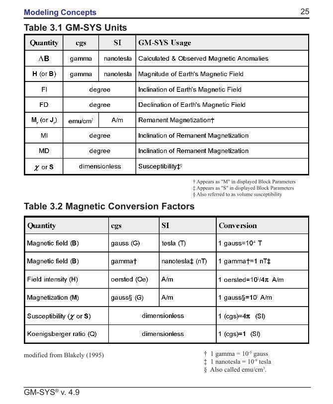
Table 3.1 GM-SYS Units
† Appears as "M" in displayed Block Parameters‡ Appears as "S" in displayed Block Parameters§ Also referred to as volume susceptibility
Table 3.2 Magnetic Conversion Factors
† 1 gamma = 10-5 gauss‡ 1 nanotesla = 10-9 tesla§ Also called emu/cm3.
modified from Blakely (1995)
26
GM-SYS® v. 4.9
Modeling ConceptsSI
B = µ0(H + M)J = µ0M
where µ0 = 4π x 10-7H/m is the permeability of freespace.The magnetization M is the vector sum of the in-duced and remanent components of magnetization:cgs and SI
M = Mi + Mr
Induced magnetization aligns with the direction ofthe Earth's magnetic field H and is proportional tothe magnetic susceptibility χχχχχ so thatcgs and SI
Mi = χχχχχH
The relative importance of remanent magnetizationto induced magnetization is expressed by theKoenigsberger ratio, Q:
Q=|Mr| / |Mi|
Note that B, H, J and M are vector quantities in thedefinitions above.In GM-SYS, the vector direction for Mr (or Jr) isinput by the user as the remanent inclination (MI)and declination (MD) in Block Parameters. The vec-tor direction for H is input by the user as the inclina-tion (FI) and declination (FD) of the Earth's mag-netic field. The calculated and observed anomaliesin GM-SYS are defined as the magnitude of theanomalous component of B in the direction of theEarth's field direction. This is often referred to asthe total-field anomaly (∆B).
GM-SYS uses the following cgs and SI units (seeTable 3.1):
To convert between SI units and cgs units, use Table3.2 (modified from Blakely, 1995). For example,divide magnetization expressed in A/m by 103 to cal-culate the magnetization in gauss.
Table 3.3 Example Susceptibilities
modified from Dobrin and Savit (1988)
27
GM-SYS® v. 4.9
Modeling ConceptsNotes:1. Although susceptibility is dimensionless, it dif-
fers by a factor of 4π between the two systems.2. The defining equations in this table require
Earth's magnetic field values to be given in oer-sted (cgs) or A/m (SI). However, in the geo-physical literature, the Earth's magnetic fieldvalues are commonly given in gammas (cgs) ornanotesla (SI). GM-SYS expects gammas (cgs)or A/m (SI).
Some traditional geophysical references (e.g., Dobrinand Savit, 1988) list susceptibilities and magnetiza-tion in mcgs units (1µcgs = 10-6 cgs). Simply divideµcgs units by 106 to use in GM-SYS. Some examplesof measured susceptibilities using cgs, µcgs and SIunits are provided in a table on the following page.Note the wide range of susceptibilities for each rocktype.
More extensive measurements of magnetic proper-ties may be found in Carmichael (1982) and Clark(1966). For a more detailed description of magneticunits, conversions, rock magnetism and theory, seeShive (1986), Grauch, et al. (1993), and Blakely(1995).
3.12 GRAVITY UNITSBy default, GM-SYS uses the Gaussian (cgs) sys-tem of units for gravity terminology (gravitationalacceleration and density). The user may choose todisplay using International System (Le Système In-ternational d'Unités or SI) units by selecting the ap-propriate option in the Display Menu. Selecting Usemicro-cgs units in the Display Menu will cause
GM-SYS to use cgs units for gravity terminologyand µcgs units for magnetic terminology. Geophysi-cal literature is currently in a state of transition be-tween cgs units and SI units. Many geophysicistscontinue to use cgs units although SI units do appearin the literature.
By default, gravity anomalies are displayed in mGalfor both cgs and SI, but you may toggle betweenmGal or µGal by right-clicking on the Gravity Axisand selecting Change Units.
The cgs unit of acceleration is cm/sec2, often referredto as the Gal (short for "Galileo"), where 1 Gal = 1cm/sec2. The geophysical literature commonly re-ports gravitational attraction in units of mGal (1 mGal= 10-3 Gal). The SI unit of acceleration is m/sec2.The cgs unit of density is gm/cm3 and the SI unit ofdensity is kg/m3. GM-SYS expects gravity values tobe in mGal and densities to be in gm/cm3 or kg/m3.To convert between SI units to cgs units, use the con-version table below. For example, divide densitiesreported in kg/m3 by 103 to calculate the densities ingm/cm3. The density for each block in a GM-SYSmodel appears as "D" when the block parameters aredisplayed.
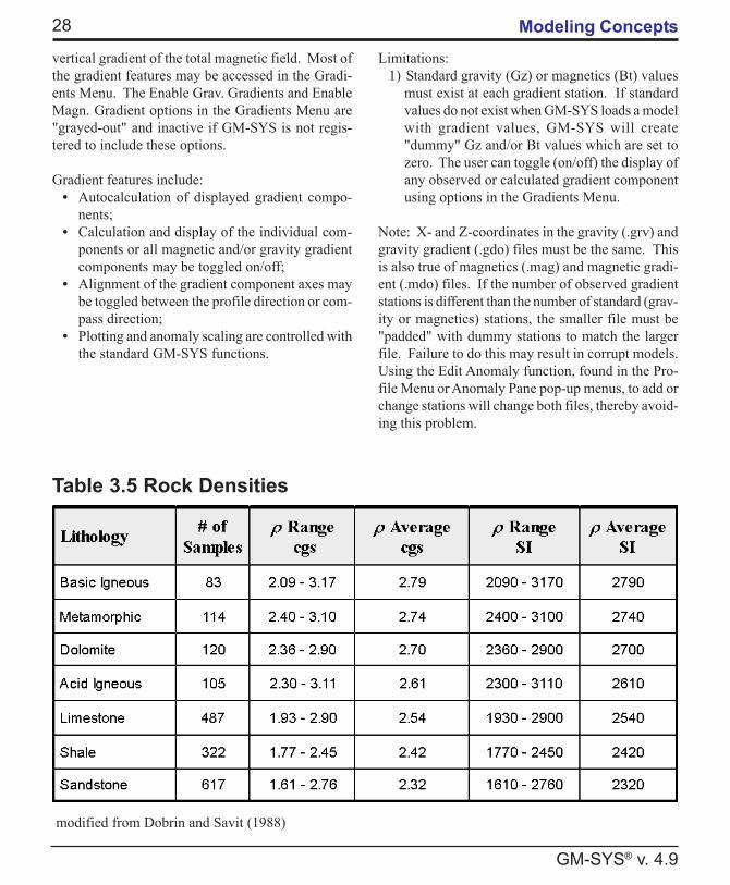
Some examples of measured rock densities using cgsand SI units are provided in Table 3.5 shown below.
3.13 GRAVITY & MAGNETICGRADIENTSThe GM-SYS Gravity/Magnetic Gradient optionadds the capability to calculate any or all of six gra-dient tensor components of the gravity field and the
Table 3.4 Gravity Conversion Factors
28
GM-SYS® v. 4.9
Modeling Conceptsvertical gradient of the total magnetic field. Most ofthe gradient features may be accessed in the Gradi-ents Menu. The Enable Grav. Gradients and EnableMagn. Gradient options in the Gradients Menu are"grayed-out" and inactive if GM-SYS is not regis-tered to include these options.
Gradient features include:• Autocalculation of displayed gradient compo-
nents;• Calculation and display of the individual com-
ponents or all magnetic and/or gravity gradientcomponents may be toggled on/off;
• Alignment of the gradient component axes maybe toggled between the profile direction or com-pass direction;
• Plotting and anomaly scaling are controlled withthe standard GM-SYS functions.
Limitations:1) Standard gravity (Gz) or magnetics (Bt) values
must exist at each gradient station. If standardvalues do not exist when GM-SYS loads a modelwith gradient values, GM-SYS will create"dummy" Gz and/or Bt values which are set tozero. The user can toggle (on/off) the display ofany observed or calculated gradient componentusing options in the Gradients Menu.
Note: X- and Z-coordinates in the gravity (.grv) andgravity gradient (.gdo) files must be the same. Thisis also true of magnetics (.mag) and magnetic gradi-ent (.mdo) files. If the number of observed gradientstations is different than the number of standard (grav-ity or magnetics) stations, the smaller file must be"padded" with dummy stations to match the largerfile. Failure to do this may result in corrupt models.Using the Edit Anomaly function, found in the Pro-file Menu or Anomaly Pane pop-up menus, to add orchange stations will change both files, thereby avoid-ing this problem.
Table 3.5 Rock Densities
modified from Dobrin and Savit (1988)
29
GM-SYS® v. 4.9
Modeling Concepts2) Both the standard gravity (Gz) curve and grav-
ity gradient curves are plotted in the gravityanomaly window. Similarly, the total field andmagnetic gradient curves are plotted in the mag-netic anomaly window. In each window, thegradient components are color-coded with a leg-end displayed in the upper-left corner of theanomaly window. A question mark (?) appearsnext to the legend items if the calculated curvehas not been updated to reflect changes in thegeologic model; i.e., "?" serves as a "modelchanged" flag. The legend entry for a compo-nent is only visible when display of the compo-nent is enabled.
3.13.1 Gradient Axis
The "Profile/Compass" Axis toggle in the GradientsMenu allows the user to change the alignment of theX-axis for gradient calculations. The X-axis for gra-dient calculation defaults to being coincident withthe profile azimuth (PROFILE). The COMPASS op-tion forces the X-Direction in the gradient calcula-tions to be due East (90°). The Profile Azimuth mustbe set correctly, relative to True North, for this op-tion to function properly.
3.13.2 Magnetic Gradient Display and Units.
The total magnetic field (Bt) and the vertical gradi-ent (Btz) are both displayed in the magnetic anomalywindow. Display of the calculated and observed gra-dient data may be toggled on and off in the Gradi-ents Menu. GM-SYS stores magnetic gradient val-ues internally in units of gammas/meter, althoughunits may be displayed and edited in units of gam-mas/meter, gammas/kilometer, nT/meter, or nT/ki-lometer. The units used may be changed by activat-ing the Magnetic Anomaly axis pop-up menu (seeSection 5.3.8.3) and selecting the appropriate unitsfrom the secondary pop-up menu.
3.13.3 Gravity Gradients Display and Units
"Normal gravity" (Gz) and six gradient tensorcomponents are displayed in the gravity anomalywindow.
• vertical gradient of the vertical component ofgravity (zz);
• gradient in the X direction of the X componentof gravity (xx);
• gradient in the Y direction of the Y componentof gravity (yy);
• gradient in the X direction of the verticalcomponent of gravity (zx);
• gradient in the Y direction of the vertical com-ponent of gravity (zy).
• gradient in the X direction of the Y componentof gravity (xy);
The individual gradient components can be toggledon and off in the Gradients Menu. Gradient valuesare input and displayed in Eotvos Units.
3.14 GRID OUTPUTThe Grid Output Option allows you to calculate theresponse of your model over an area and generate aGeosoft grid (.grd) file as output. If the model in-cludes a coordinate transformation in the ECS file,the output grid will use the original ground units andwill be correctly rotated.
You may elect to calculate the gravity or magneticgrid response, or one of the gradient components ifthe Gradients Option is licensed. Calculate the re-sponse at a specified constant terrain separation orconstant elevation. Enter minimum and maximumX and Y limits and the grid cell size, or accept thedefault limits, which are determined from the PlanView extents.
30
GM-SYS® v. 4.9
Modeling Concepts
3.15 SYMBOL DISPLAYImport one or more ASCII files with X, Z coordi-nates, optionally including symbol index, dip and sus-ceptibility fields, and display symbols over the CrossSection pane. Each symbol file may be configuredindependently to associate symbol indices with sym-bol type, color, line weight, and size. Each symbolfile may be toggled on/off independently. Entries ina symbol file that enclude dip and susceptibility fieldswill plot with ‘dip-tails’ scaled by susceptibility.
Use Symbol Plotting to display dip measurements,depth-solutions from NGA’s Depth-to-BasementGXs, shotpoint locations, tie-line crossings, inter-preted seismic horizons, and more. GM-SYS comeswith a set of default symbols in gmwin.sdf, the sym-bol definition file. Use the predefined symbols, oradd your own. Symbols do not affect GM-SYS cal-culations in any way.
3.16 WELL DISPLAYGM-SYS incorporates two types of wells, the stan-dard GM-SYS well markers and LAS well files (v.1.2 and 2.0). Like symbols and bitmaps, wells pro-vide visual aids to modeling and do not affect com-putation of the model response. You may assign apredefined well symbols, or add your own symbols.LAS wells may display up to two log curves withuser-configured scale, color and line weight. Usewell markers to mark depth(s) to known horizons.
3.17 BITMAP DISPLAYThe Seismic Bitmap Option enables GM-SYS to dis-play bitmaps in the background of the cross sectionpane for use as a modeling aid. Bitmaps may be seis-mic depth sections, scanned cross sections, depth-to-basement picks; any image that may be registeredin GM-SYS model space (i.e. XZ coordinates, whereZ is depth). Although not all formats have beentested, the ImageMagick convert program incorpo-rated into the GM-SYS distribution should read thefollowing image formats without additional “helper”applications:
BMP Microsoft Windows bitmap imageBMP24 Microsoft Windows 24-bit bitmap imageCMYK Raw cyan, magenta, yellow, and black bytesDCX ZSoft IBM PC multi-page PaintbrushDIB Microsoft Windows bitmap imageFAX Group 3 FAXFITS Flexible Image Transport SystemG3 Group 3 FAXGIF CompuServe graphics interchange formatGIF87 CompuServe graphics interchange format
(version 87a)GRAY Raw gray bytesICB Truevision Targa imageICO Microsoft iconJBG Joint Bi-level Image experts Group interchangeJBIG Joint Bi-level Image experts Group interchangeJPG Joint Photographic Experts Group JFIFJPEG Joint Photographic Experts Group JFIFJPEG24 Joint Photographic Experts Group JFIFMIFF Magick image formatMONO Bi-level bitmap in least-significant-byte
first orderP7 Xv thumbnail formatPBM Portable bitmap format (black and white)PCD Photo CDPCDS Photo CDPCL Page Control LanguagePCT Apple Macintosh QuickDraw/PICTPCX ZSoft IBM PC PaintbrushPIC Apple Macintosh QuickDraw/PICTPICT Apple Macintosh QuickDraw/PICTPICT24 24-bit Apple Macintosh QuickDraw/PICTPGM Portable graymap format (gray scale)PMX Windows system pixmap (color)PNG Portable Network GraphicsPNM Portable anymapPPM Portable pixmap format (color)PSD Adobe Photoshop bitmapPTIF Pyramid encoded TIFFPWP Seattle Film WorksRAS SUN RasterfileRGB Raw red, green, and blue bytesRGBA Raw red, green, blue, and matte bytesRLA Alias/Wavefront imageRLE Utah Run length encoded imageSFW Seattle Film WorksSGI Irix RGB imageSUN SUN RasterfileTGA Truevision Targa imageTIF Tagged Image File FormatTIFF Tagged Image File FormatTIFF24 24-bit Tagged Image File FormatTTF TrueType fontVDA Truevision Targa imageVST Truevision Targa imageX X Image
31
GM-SYS® v. 4.9
Modeling ConceptsXBM X Windows system bitmap (black and white)XPM X Windows system pixmap (color)XV Khoros Visualization imageXWD X Windows system window dump (color)
32
GM-SYS® v. 4.9
Modeling Concepts
33
GM-SYS® v. 4.9
Model Elements
4. MODEL ELEMENTS
A GM-SYS model hasfour main components;the structural (geo-logic) model, addi-tional external data (i.e.wells, symbols, back-drops, and LAS wellcurves), gravity sta-tions and magnetic sta-tions. These featuresare illustrated in thesimple model at left.You may change the default symbol and line colors,sizes, and weights, and fonts in the Preferences dia-log accessed from the File Menu.
Conceptually, the model is a 2-D or 2¾-D cross sec-tion extending to infinity to the left (-X) and theright (+X). The Z-axis of the cross section displaysdepth (i.e. Z is positive down). Areas of constantdensity and magnetic properties are delineated byclosed polygons separated by surfaces defined by twoor more points. In 2-D models, these polygons, or"blocks" extend to infinity in the third dimension (±Y)into and out of the screen or page. In 2¾-D models,these blocks may be truncated at a given distancefrom the plane of the profile.
4.1 SURFACESTo GM-SYS, themodel is actuallycomposed of linesthat define the sur-faces between areasof differing density ormagnetic properties. You are able to change the sur-faces by moving, deleting, and adding points thatdefine these boundaries. The top of a model is asurface which defines the topography of the crosssection. The default colors are green for 2-D sur-faces and dark green for 2¾-D surfaces.
Horizons are one or more contiguous surfaces con-nected end-to-end (no branching).
4.2 POINTSA surface is defined by a series of two or more pointsor vertices. Straight linesegments connectingthese points make up thesurfaces.
4.3 BLOCKSA polygon, or a block, isan area of constant den-sity and magnetic prop-erties and strike (Y) extent. The parameters of a blockare the name, the density, the susceptibility (whichcombined with the Earth's magnetic field gives theinduced component of the magnetic anomaly causedby a block), the magnitude, declination and inclina-tion of the remanent magnetization, and velocity.Blocks also may be given a fill pattern with fore-
34
GM-SYS® v. 4.9
Model Elementsground and/or back-ground color for displayand plotting purposes.
If the block is 2-D, theseproperties extend to “in-finity” in the +Y and -Ydirections. If the blockis 2¾-D, the “main”block has a +Y and/or -Y limit and the “block” ex-tending from this limit to infinity may be assigneddifferent properties from the “main” block. You mayelect to assign separate fill pattern and/or color tothe “+Y-” and “-Y-blocks”, which will only be dis-played in the Plan View.
4.3.1 Block Labels
Each block is assigned a name, which may bechanged with the Examine option or within the BlockParameter spreadsheet.When the Block Labelsoption in the DisplayMenu is toggled on, allblock names are dis-played. You may togglethe display of individualblock labels off in theExamine Block dialog. Note: the default positionfor a block name is the center of the block. A labelfor a newly-created block (e.g. using Split Block)may default to a position outside of the current view.
Block labels may be moved using the Move Labelcommand, found in the Action Menu or the ActionTool Box (Section 5.1.7). To move the label for anewly-created block on-screen, activate the MoveLabel command and select "Snap Mode". Click themouse within the new block to move the label to thatpoint.
4.3.2 Block Data
Each block has a density, susceptibility, remanentmagnetization, and velocity assigned to it. If theblock is 2-D, these properties extend to “infinity” inthe +Y and -Y directions. If the block is 2¾-D, it hasa +Y and/or -Y limit and the “block” extending fromthis limit to “infinity” may be assigned other proper-ties. Information for the -Y and +Y- portions of a2¾-D block are not displayed, but may be viewedand changed using Examine Block or within theBlock Parameter spreadsheet. Surfaces surroundingblocks with 2¾-D limits are displayed with a differ-ent color in the cross section and plan view (defaultis olive). You may change the default color or linestyle in the Preferences.
If either or both of the Grav. Info or Magn. Info op-tions in the Display Menu are checked, the informa-tion for the “main” block is displayed beneath theblock label for each block. Magnetic remanence pa-rameters are only displayed if the remanent magne-tization is non-zero. By default, density, susceptibil-ity, and remanence values are displayed to three sig-nificant figures, but this may be changed in the Pref-erences.
4.4 BACKDROP IMAGESBackdrop images are used as a visual aid to modelconstruction, but do not affect the computations per-formed by GM-SYS. GM-SYS will import a widevariety of image formats with the Seismic Bitmapoption. If an image is too large to load, the user mayelect to have GM-SYS scale the image to a moremanageable size.
By default, the image will be scaled to fill the cur-rent cross-section view. If you know the approxi-mate coordinates of the image corners, you mayspecify these values when loading the image. Oncethe image is loaded, use the Register Backdrop func-tion to precisely register the image.
35
GM-SYS® v. 4.9
Model Elements
The Register Backdrop function allows you to pre-cisely scale the loaded image by assigning modelcoordinates (X,Z) to two pixel lo-cations in the image.
4.5 SYMBOLSSymbols are another visual aid thatdoes not affect the computations.Use symbols to show the locationsof depth-to-basement picks, strike& dip measurements, seismic ho-rizons, or any other reference lo-cation that might aid in your modeldevelopment or presentation.
Symbol files are space-delimitedASCII files that contain X, Z, asymbol flag, and optionally dip andsusceptibility values for each symbol location. Mul-tiple symbol files may be displayed in a model andeach may be configured independently.
The available symbols are defined in gmwin.sdf, thesymbol definition file. You may add symbol defini-tions by editing this file with a text editor.
4.6 WELL MARKERS AND LASWELL FILESWells are used as a type of annotation, but are notused in the computations performed by GM-SYS.GM-SYS allows two types of wells, the standard wellmarkers and LAS well files (v. 1.2 and 2.0).
By displaying a well marker, you can show depthsof various stratigraphic horizons or other geologicalmarkers. This data can come from well logs, coresamples, magnetotellurics, resistivity studies, geo-logic maps, or any other source you may have. It isuseful to have these annotations on the screen to keeptrack of all of the geological and geophysical con-straints on the model.
The locations of well horizons are stored as depthbeneath the ground surface (see Section 7.8) andmay be edited from the Profile Menu (Section5.1.3).
Each LAS Well file may be independently config-ured to show up to two log curves. Specify thewell location, symbol, and up to two log curves fordisplay. Configure scale, color, and line weight foreach curve.
4.7 GRAVITY AND MAGNETICSTATIONSThe observed gravity and magnetics profiles are com-posed of stations. These stations are the locationswhere gravity and/or magnetic measurements havebeen made and where the model response will becalculated. Gravity stations generally lie on the to-pography of the model if they are land-based gravityreadings. Magnetic stations may be on land or atsome altitude, in the case of an aeromagnetic survey.When GM-SYS calculates the gravity or magneticresponse of a model, it will calculate and plot thetotal response of the model at each station. The ob-served response at each station over the cross sec-tion will also be plotted. This will allow you to modela cross section to match existing data.
Actual observed data are not necessary for the use ofGM-SYS, but would normally be used when fittinga cross section to observed data. If observed dataare unavailable, dummy station locations must beentered as calculation points.
36
GM-SYS® v. 4.9
Model Elements
37
GM-SYS® v. 4.9
GM-SYS Interface
5. GM-SYS INTERFACE
The GM-SYS interface consists of a menu system,Menu Tool Bar, the Action Tool-Box, the ModelSpace, and the Status Bar. The Model Space maycontain one or more models in separate Model Win-dows. GM-SYS is most commonly used as a stand-alone application, but may be run in linked mode fromwithin OASIS montaj.
5.1 MENUSWhen GM-SYS is started without specifying an ini-tial model, only three menus with limited options areavailable: the File Menu, Window Menu and theHelp Menu. The menu system expands to includeadditional options when a model is loaded. Many ofthe menu options may also be found in the context-sensitive pop-up menus described in Section 5.3.8.
38
GM-SYS® v. 4.9
GM-SYS Interface5.1.1 File Menu
The File Menu controls file access, printing and plot-ting functions. The New Model…, Open Model…and Save Model options are also accessible from theMenu Tool Bar.
New Model and Open Model
The New Model… option activates the New ModelCreation dialog (discussed in Section 2.3), whichguides you through the creation of a starting model.The Open Model… option allows you to open anyGM-SYS model (default extension .sur).
Save Model and Save as
The Save Model and Save as… options overwritethe previous version of the model or allow you tochoose a new or different model name, respectively.For the Save as… option, if a model name is alreadyin use, GM-SYS prompts you with a message askingwhether you wish to overwrite the existing model.Models are saved in a group of eight to ten files withthe same name and various extensions (See Section7). Hence, it is not recommended that you save mod-els with an extension other than .sur.
Close
The Close option closes the active model, promptingyou to save any changes that have occurred since thelast Save Model command. Models may also be
closed using the controls embedded in the window-dressing of the Model Window.
Preferences
The Preferences... option allows you to personalizeyour GM-SYS environment. Preferences can be setfor file locations, the model window, and miscella-neous items.
In the Files dialog you may select default locationsfor your model files, backdrop images, and backupfiles generated by the AutoSave feature. WithAutoSave enabled, GM-SYS will save all open modelfiles at the user-specified interval. In the event of asystem failure or power outage, these files may berecovered during the next GM-SYS session. Thebackup files are deleted when GM-SYS exits nor-mally.
The Model Windows preference selection includesthe following three dialog menus: Fonts, Anomalies,and Cross Section.
The Fonts dialog allows you to specify fonts usedfor each part of the GM-SYS display.
The Anomalies dialog allows you to set the color,line style, and weight of each data component in theanomaly display. You may also specify whether eachcomponent’s observed data and/or calculated curveis displayed by default when GM-SYS opens.
39
GM-SYS® v. 4.9
GM-SYS InterfaceThe Cross Section dialog allows you to configurethe color, line style, and weight of the line elementsthat comprise the Cross Section display. You mayalso set the number of decimal places to use whendisplaying density, susceptibility, or remanent mag-netization values; these values apply to the Anomalyspreadsheet, as well.
In the Miscellaneous dialog, you may set the maxi-mum number of “Undos” and “Previous Views”saved for each model during a modeling session. Youmay select the default units GM-SYS will use, whichmay be overridden on a model-by-model basis.
Beginning with GM-SYS version 4.6, extensions andchanges have been introduced to the .BLK, .SUR,.ECS, and .GMS file formats. By default, GM-SYSuses the new formats when saving a model. If youwish to remain compatible with earlier versions ofGM-SYS, you may uncheck this box. Your modelswill not retain block color/pattern information andwill not load bitmap files or symbol files. Some largemodels may fail to load with a “Too many Surfaces”error message.
Print
The Print… option generates a precisely-scaled plotof your model for printing or importing into graph-ics applications. The Print dialog, discussed in Sec-tion 6, allows you to set the vertical scale of eachpane and the model horizontal scale, vertical exag-geration, and model and axis headings. You mayspecify font sizes and font styles. GM-SYS con-structs an outline preview of the model layout priorto printing directly to the installed printer or to a filefor printing later.
Exit
The Exit option will close all open model windowsand terminate GM-SYS. You will be prompted tosave changes to each open model before it is closed.
You may also exit GM-SYS by using the controlsembedded in the Main Window window-dressing.
Previously Opened Model List
GM-SYS maintains a list of previously-opened modelfiles at the bottom of the File Menu. You may openany of the listed models by selecting the model namefrom the list. The number of saved file names maybe configured in the Preferences.
5.1.2 View Menu
To GM-SYS, a View is a storedset of coordinates specifying theboundaries of the Model,Anomaly, and Plan View panesand the depth of the Plan View.Views are useful when you wishto repeatedly edit or plot the sameportion of the model. Using thefunctions built into the ViewMenu you may save, edit, replace, and delete views,change to a previously saved view, and change theorder of saved views.
Previous View
The Previous View option allows you step backthrough a stack of saved or unsaved views generatedduring the current editing session. Separate viewstacks are constructed for each model opened duringan editing session. A view is placed on the stackwhenever the zoom functions are used or the rangeof any pane in the Model Window is changed. Thenumber of views remaining in the stack is displayedas part of the Previous View option. By default,GM-SYS will hold up to 20 views in the stack. Thedepth of the stack can be changed inFile|Preferences...|Miscellaneous. The Previous Viewstack for a model is cleared when you close the modelor exit GM-SYS.
40
GM-SYS® v. 4.9
GM-SYS InterfaceMark Current View
When the range of the display is changed by utiliz-ing a scroll bar, GM-SYS does not automatically savethe view on the Previous View stack. Selecting MarkCurrent View will explicitly place the current viewon the stack.
Add Current View
This option allows you to save the current view atthe bottom of the View List, without having to specifya name. The view name will default to "New View#?" where "?" is the position of the view in the list.You may change the name or any other parametersof the view using the Edit Views option.
Edit Views
The Edit Views option activates the View List dia-log. The View List dialog allows you add, delete, orchange views in the list that appears at the bottom ofthe View Menu.
The Up and Dn buttons allow you to reorder yourview list; e.g. you could move the "Salt Dome" viewto the top (default) position. When an existing viewis highlighted, the Edit button activates the View dia-log (following page). This dialog allows you tochange the name and/or the limits of each pane in
the Model Window for that view. Use the Repl. W/CView button to replace the highlighted view withthe current screen configuration.
To add a new view, first arrange your display by set-ting the limits for each pane or by using the scrollbars. Then select Edit Views from the View Menuand choose the Add Current View button. The Viewdialog will display the "New View" with the param-eters set to the current screen configuration. Adjustthe values if necessary, give the view a new nameand click "OK." The new view will be added to thenumbered list. You may then reorder the views ifyou wish.
View List
The first view in the list, named "Start up" by de-fault, is the initial view displayed when you open themodel. The "Infinity" view, listed second by default,shows you the entire model, extending from -30,000km to +30,000 km along the profile axis.
41
GM-SYS® v. 4.9
GM-SYS Interface5.1.3 Overlay Menu
The Overlay Menu controlsmodel elements which pro-vide a visual guide to modelbuilding or otherwise en-hance the appearance of yourmodel, but do not affect cal-culations.
Backdrop
This Intermediate function allows you to place a reg-istered bitmap image in the background of the cross-section pane of the model. The image may be a depth-scaled seismic section, a geologic cross sectionscanned from a publication, a hand sketch, or anyother image that aids in development of your model.
Enable Backdrop
The Enable Backdrop selection toggles on/off the dis-play of the backdrop image. This selection must beset on to display a backdrop image. You may alsoset this toggle in the Backdrop Image Setup dialogdescribed below.
Load Backdrop
Selecting Load Backdrop will bring up the "Back-drop Image Setup" dialog, as shown below. If youchoose a file type other than BMP, GM-SYS usesImageMagick to import the image. A thumbnail ofthe image will be displayed after it has been loaded.
Initially, the image will be scaled to approximatelyfill the current View. To adjust the position of theimage in the cross-section pane, enter the User Co-ordinates to match the outside edges of the image.Make sure the Enable Backdrop box is checked be-fore you click “OK.”
Backdrop Registration
You may fine-tune the image registration by assign-ing model coordinates to two locations in the image,using the procedure outlined below. Using locationsnear opposite corners of the image works best.
1) Zoom to the first registration point, if necessary.Right-click in the Cross Section pane to display apop-up menu with the Register Image option. Se-lect the 'Select 1st Reg. Point' item from the pop-up submenu. The '1st Reg. Point' window will ap-pear, as shown below.
2) Click on the new registration point on the image.Its current model coordinates will be displayed inthe dialog. Enter the new coordinates and click 'OK'.
3) Zoom to the 2nd registration point, choose '2ndreg. point' from the pop-up menu, and repeat theprocess.
4) Select 'Apply registration to image' from the Reg-ister Image pop-up menu to apply the new regis-tration information.
42
GM-SYS® v. 4.9
GM-SYS InterfaceSymbols
Point data, such as depth-to-basement picks, seismichorizon picks, and shot-point or tie-line locations,may be loaded and displayed as symbols over yourmodel. Files may contain Profile (X,Z) or Real-World(X,Y,Z) coordinates; GM-SYS assumes that the co-ordinate system and projection of the file match thatof the model.
Load and configure each symbol file independently.Select from a list of pre-defined symbols, or add yourown symbols, and customize color, size, and lineweight. Depth-to-basement picks may be plotted withdip-tails whose length is proportional to the appar-ent susceptibility.
Enable Symbols
The Enable Symbols selection toggles the display ofall loaded symbol files. Regardless of how may sym-bol files are loaded and toggled on (see below), thisoption must be toggled on to display any symbols.
Load/Config Symbols
The Load/Config Symbols option brings up the Sym-bol Manager dialog. Here you may load, delete, orreload one or many ASCII files containing (X,Z) or(X,Y,Z) locations to be displayed as symbols overyour model. You may elect to show/hide each loadedsymbol file independently and each loaded file maybe configured independently.
A symbol file may contain several different types ofinformation (e.g. depth to basement picks, shot points,etc.). Each line of the symbol file should containcoordinates for the symbol, a symbol flag, and mayoptionally include dip, and susceptibility fields. Thesymbol flag should be a positive integer that is thesame for all points containing the same type of infor-mation. Dips should be in degrees. Susceptibilityunits may be either cgs or SI; the length of the dip-tails will be scaled logarithmically with values of 10-7
scaled to the effective radius of the symbol.
The symbol configuration dialog allows you to asso-ciate the symbol flag field in your symbol files withpredefined symbols. If any symbols in a file containonly X,Z fields, all symbols in that file will be as-signed the flag value #00. Each flag value may beassociated with a specific symbol type, size, color,and line weight. Symbol files that include dip andsusceptibility information will plot with ‘dip tails’scaled to the susceptibility.
Edit Wells
Well markers show the locations of borings and for-mation tops in the Cross Section and Plan View panes.Wells are located in model coordinates; i.e. X-Dis-tance along the profile and Z-elevation of the groundsurface (Z is positive down). Well horizons are in-put as depth below ground surface and should al-ways be positive. Units for X, Z, and depth to hori-zons may be independently selected using the pop-up menus in the Edit Well dialog box.
Enable Wells
This option toggles the display of all Well markers.
Add/Config Wells
You may add, delete, or modify well markers thatappear in the Cross Section and Plan View panes.Select one of the existing wells to edit, or click theNew button and create a new well.
43
GM-SYS® v. 4.9
GM-SYS InterfaceLAS Wells
LAS well files (v. 1.2 and 2.0) may be loaded andone or two curves displayed in your model. You mayconfigure line color, weight, style, and scale for eachselected curve. Well symbols may be selected froma list of pre-defined symbols, or you may add yourown well symbols.
Enable LAS Wells
The Enable LAS Wells selection toggles the displayof all loaded LAS well files. Regardless of how mayfiles are loaded and toggled on (see below), this op-tion must be toggled on to display any LAS wells.
Load LAS Wells
The Load LAS Wells option activates the LAS Wellconfiguration dialog. Here you may load, reload,and delete LAS well files. You may elect to show/hide each loaded LAS well file independently andeach loaded file may be configured independently.
LAS well files may contain one or more log curves.Once you have specified X, Y, and elevation coordi-nates for a loaded well, you may configure up totwo log curves for display, specifying line color, lineweight, and scale for each. Scaling of curves fits aspecified range of values (e.g. 0 - 3.0 g/cc) into aspecified range of distance from the well location(e.g. 2 - 8 km).
Block Fill
GM-SYS allows you to specify a block-fill pattern,a pattern color (the foreground color), and a back-ground color independently for each block. Usingthis menu, you may elect to display no fill, only theforeground pattern (fill is “transparent”), or bothforeaground and background colors on a global ba-sis (all blocks). You may elect to scale the blockforeground colors by mapping a color table to rangesof block density, susceptibility, or remanent magne-tism. Use the Examine Block command tool to con-trol block transparency on an individual basis.
Enable Block Fill
This selection toggles on/off the display of block fillin the Cross Section and Plan View panes. This togglecan also be accessed in the Display menu and theCross Section pop-up menu. If Enable Block Fill isnot selected, the three following items do not appearin the Image menu.
Block Foreground Color
The Block ForegroundColor option displays a pop-up menu that allows the userto select one of four choices for selecting the fore-ground color. The first selection, "Color Blocks asNormal" selects the block-fill color and pattern asset via the Examine Block function or via the BlockParameter spreadsheet. The other three selectionsutilize the color schemes defined via the Color Tooloption described below. Note that the Density, Sus-ceptibility, and Magnetization color schemes only af-fect the foreground colors. The background colorsare set via the Examine Block function or the Blockspreadsheet and modified as described below.
Block Background Color
The Block BackgroundColor option displays apop-up menu that allows the user to modify the waybackground colors are displayed. “Fill Blocks as Nor-mal” uses the background color and transparency asspecified by the user for each block. “Force BlocksTransparent” overrides the user’s transparency set-tings and makes all blocks transparent. “Force BlocksSolid” fills all blocks with the current foregroundcolor.
Color Tool
The Color Tool selec-tion displays a dialogthat allows the user toassign color tables toranges of block prop-erties (density, suscep-tibility, magnetization,
44
GM-SYS® v. 4.9
GM-SYS Interfaceand velocity. Each block property may use a differ-ent color table. Users can import ASCII color tablesin the standard Geosoft RGB or CMYK formats. Ex-ported color tables are Geosoft RGB color tables.
5.1.4 Display Menu
The Display Menu is a selectionlist that allows you to toggle on/off all of the model elements thatappear in the Cross Section,Anomaly, and Plan View panes;with the exception of the modelsurfaces. The Action Tool Boxand Single Block Response curvesmay be toggled on/off from thismenu. Select either cgs, micro-cgs, or SI units for block param-eter and anomaly display from thismenu.
The Display Menu is organizedinto sections the Gravity Anomaly,Magnetic Anomaly, and Cross Section panes. GM-SYS displays the same model elements in the PlanView pane as in the Cross Section pane. Optionswhich affect the display of magnetic and gravitycurves may be accessed using the Magnetic and Grav-ity Anomaly pop-up menus as well. All other op-tions may be accessed using the Cross Section pop-up menu.
Display Menu options affect all open models. Dis-play toggles affect all Model Window panes and con-trol the appearance of model elements on plot out-put.
5.1.5 Profile Menu
Parameters which affectcalculation of the gravityand/or magnetic responseof the entire model profilemay be found under theProfile Menu. GM-SYS re-quires that the magneticfield parameters, the profileazimuth, and the relativestrike angle be set in orderto accurately calculate the model's magnetic response.The relative strike angle must be set to properly cal-culate the gravity response of the model.
Set Mag. Field
Use the Set Mag Field option to input the Earth'smagnetic field intensity, inclination, and declinationat the location of your survey and model.
If you do not have NGRF, this information may beobtained from a variety of published sources. Mapsshowing magnetic field data may be found in manygeophysical text books (e.g., Merrill and McElhinny,1983, Fig. 2.2, and Dobrin and Savit, 1988, Fig. 15-7 and 15-8), or from one of the numerous map seriesavailable from the USGS (e.g., Fabino, 1983, a,b,c).If you do not have access to these more accuratesources, the field may be approximated by the Earth'sdipole field.For that approximation:
Dipole field intensity:H = 31,200 * (1+ 3sin2 (lat))½ (gammas)
Dipole field inclination:FI = tan -1 ( 2tan (lat))
Dipole field declination:FD = 0.0
where "lat" is the latitude of the observation point.GM-SYS defaults to values of 56,000 gammas, 60°,and 20° for the magnetic field intensity, field incli-
45
GM-SYS® v. 4.9
GM-SYS Interfacenation, and field declination, respectively. This op-tion may also be accessed from the MagneticAnomaly pane pop-up menu.
Set Azi./Strike Angle
Set the Profile Azimuth to correctly orient your modelwith respect to the geomagnetic field. Both positiveand negative entries are acceptable (e.g., a NW pro-file azimuth may be represented by 315° or -45°).
If your model strike is oblique to the profile azimuth,the Relative Strike Angle must be set. See Section3.5 on Skewed Models for a description of the con-ventions used in GM-SYS to describe the modelstrike. The default profile azimuth and relative modelstrike are 90° (West to East) and 90° (orthogonal),respectively. The Set Azimuth/Strike Angle optionis also available in the Plan View pane pop-up menu.
Set Real-World Origin Coord.
GM-SYS uses a profile-based coordinate system, inwhich the model and gravity/magnetic observationpoints are located along a straight line. Models cre-ated from within Oasis montaj, using XYZGMS, orby import using CVTGMS may have a coordinatetransformation associated with the model that allowsmapping of the profile coordinates to “Real WorldCoordinates,” in which the profile origin (X=0, Z=0)is assigned X,Y,Z coordinates. Use this function ifyou have created a model in another way and wish toassociate the profile coordinates to some other coor-dinate system. See the description of the ECS(External Coordinate System) file for more de-tails.
Set Plan View Depth
The Plan View Depth option allows you to numeri-cally specify the depth of the horizontal slice throughthe model which is presented in the upper pane asthe Plan View. By default, the units used are thoseof the Z-axis in the cross-section display. You mayselect different units by clicking the units box andchoosing from the pop-up submenu that appears. ThePlan View depth may also be changed graphically
by using the Move Plan View Depth option in theCross Section pop-up menu.
Edit Anomaly
Activate the Anomaly spreadsheet editor by select-ing the Edit Anomaly option. Within the spreadsheeteditor, you may add or delete gravity and/or magnet-ics stations, change the along-profile position (X) orelevation (Z) of stations, or change the observed val-ues at stations. You may edit, copy, and paste cellsand add or delete rows (stations) or import new datausing the functions in the Edit Menu, which is vis-ible when the spreadsheet editor is active.
Data to be imported must be in generic, space-de-limited ASCII files. Importing any new gravity orgravity gradient data replaces all gravity and gravitygradient data. Importing any magnetic or magneticgradient data likewise replaces all magnetic and mag-netic gradient data.
NOTE: Since GM-SYS requires that gravity or mag-netics stations exist at each point where gradients arecalculated, adding or deleting gravity or magneticsstations produces a corresponding change in the re-spective gradient components, and vice versa.
Edit Wells
This option provides an additional interface to theAdd/Config Wells option in the Overlay Menu de-scribed in Section 5.1.3. It is maintained for com-patibility purposes.
Edit Blocks
GM-SYS 4.6 introduces the Block Parameter spread-sheet. To activate the Block Spreadsheet, pull downthe Profile menu and choose Edit Blocks. The pa-rameters for each block in the model are displayedas a single row in the spreadsheet. You may edit theparameters and copy and paste one or many param-eters from one block to another. This allows you toquickly and easily duplicate block parameters (copyonce, paste many) and perform quality-control onyour block parameters. The Undo function does notinclude changes to the Block Spreadsheet. You must
46
GM-SYS® v. 4.9
GM-SYS Interfacealways perform a total recalculation of the model re-sponse after making changes in the Block Parameterspreadsheet.
Magnetics Elevation Adjust
Use this option to give all magnetics stations a con-stant terrain separation. The value entered is an ab-solute height above topography; GM-SYS does notadd this value to the existing station elevations -- itreplaces them. To move all stations to the topographicsurface, enter "0". This function is useful for model-ing a magnetic survey that is draped above the to-pography. This option is also available in the Mag-netic Anomaly pane pop-up menu.
Magnetics DC Shift
This dialog allows the DC Shift to be applied in oneof three ways:
1) GM-SYS automatically calculates the DC Shiftvalue to minimize the RMS error ("Auto"),
2) by forcing the calculated curve and the observedcurve to match at some user-selected referencestation (" Station#"), or
3) by explicitly subtracting a given value from thecalculated curve ("Absolute"). GM-SYS de-faults to the "Auto" option.
In addition to entering a station number, you mayalso force the curves to match at a station by placingthe cursor on an observed data point in the anomalypane (a green dot) and clicking the left mouse but-ton. All the calculated values will be shifted by theamount necessary to make the calculated value andthe observed value agree at the station under the cur-sor. This station is indicated on the screen by twovertical arrows above and below the selected point.The point where the two values are the same can bechanged at any time by repeating the procedure.The Magnetic DC Shift dialog is also availablefrom the Magnetic Anomaly pane pop-up menu.
Gravity Elevation Adjust & Gravity DC Shift
The Gravity Elevation Adjust and DC Shift optionsoperate identically to the corresponding Magneticsoptions (see above). They are also available fromthe Gravity Anomaly pane pop-up menu.
5.1.6 Gradients Menu
The Gradients Menu controlshow gradient data in yourmodel are displayed and cal-culated. The Gradients Menuis always present, even if yourversion of GM-SYS is not configured to calculategradient responses.
Enable Grav. Gradients / Magn. Gradient
These options allow you to toggle on and off the dis-play and calculation of all gravity gradients and themagnetic gradient, respectively. If GM-SYS is notregistered to include one or both of these options,the unavailable option(s) will be "grayed-out" andinactive. If neither of these menu options is toggledon, the following menu options will not be visible.
Gradient Axis
The Gradient Axis option displays a pop-up menuthat allows the user to toggle the alignment of the X-axis for gradient calculations. The X-axis defaultsto being coincident with the profile azimuth (PRO-FILE). The COMPASS option forces the X-direc-tion in the gradient calculations to be due East (90°).The Profile Azimuth (see Section 5.1.5) must be setcorrectly, relative to True North, for this option tofunction properly.
Edit Gradients…
The Edit Gradients…option activates the Anomalyspreadsheet editor. If the Enable Grav. Gradients orEnable Magn. Gradients options are toggled on, tabswill appear in the Anomaly spreadsheet editor which
47
GM-SYS® v. 4.9
GM-SYS Interfaceallow you to edit gradient data. Within the spread-sheet editor, you may add or delete stations, changethe along-profile position (X) or elevation (Z) of sta-tions, or change the observed values at stations. Stan-dard Cut, Copy, and Paste functions are availablefrom the menu tool bar or the Edit Menu when thespreadsheet editor is active.
NOTE: Since GM-SYS requires that gravity or mag-netics stations exist at each point where gradients arecalculated, addition or deletion of a station for anygravity gradient component will produce a corre-sponding change for Gz and all gravity gradient com-ponents; and vice versa. Similarly, the addition ordeletion of magnetic gradient station(s) will producea corresponding change in the magnetics stations.
Show Gravity Gradients/Magnetic Gradients
These options activate pop-up menus that allow youto toggle on and off the display of observed data andcalculated response curves for individual gradientcomponents. These options are also available in theGravity Anomaly and Magnetic Anomaly pop-upmenus if the Enable Grav. Gradients or Enable Magn.Gradient options, respectively, are toggled on.
5.1.7 Action Menu
Commands available in the ActionMenu manipulate the geologicmodel cross section. All of thesecommands are also available in theAction Tool Box (shown at right),with the exception of the Undo func-tion (see below). Only one of thesecommands may be active at a time.The active command is denoted bya check mark in the Action Menu andas a "depressed" button on the Ac-tion Tool Box. Pressing the right mouse button priorto completion of an action will abort that action.
Undo
Select the Undo command to reverse theaction of any other command in the ActionMenu. The Undo command is actually a
stack of operations; you may undo several operationsin reverse order of their occurrence. Up to 10 opera-tions may be "undone". Undo does not update thecalculations. Be sure to click on the calculate buttonafter a sequence of Undo commands.
The Undo button resides on the Menu Tool Bar in-stead of the Action Tool Box to reduce the chance ofundoing operations by accident. Selection of theUndo command does not change the selected actionin the Action Menu and Action Tool Box.
Move Point
The Move Point command allows the userto relocate a single point. Select the pointby pointing to it with the mouse cursor and
clicking the left mouse button. Move the cursor to anew location while holding the mouse button down,then release the button. If auto-calculation is enabled,dynamic recalculation of the magnetic and/or grav-ity response will occur as the point is being moved.If multiple points lie within the search radius whenthe button is pressed, GM-SYS will beep and an er-ror message will appear in the status bar. You mayneed to zoom closer in order to isolate a single point.
In the Plan View pane, you may use the Move Pointmode to drag the ends of 2¾-D blocks and changethe strike length. When cursor-tracking is enabled,you may use this technique to drag the end of a blockin GM-SYS to match a feature in a map displayed inOasis montaj.
48
GM-SYS® v. 4.9
GM-SYS InterfaceMove Group
The Move Group command allows you tomove any number of points the same direc-tion and distance simultaneously. Multiple
points may be selected formovement using the MoveGroup radio toggle box(shown below) which ap-pears when this item is se-lected. Points may be se-lected or deselected for mov-ing in any combination ofthree ways:
Mark Point: toggle selection of individual points;Mark Block: toggle selection of all points defining
a block by clicking within a block; orMark Box: toggle all points within a window de-
fined by dragging the mouse.
To move the selected points, choose the Move Marksoption, press the left mouse button within the CrossSection pane, drag the mouse in the desired direc-tion, and release the button to complete the move.The Move Group toggle box will disappear when adifferent action is selected.
Add Point
Place the cursor on a surface where you wishto create a new point and press the left mousebutton to create a new point. If a point al-
ready exists within the search radius, GM-SYS willbeep and display a warning message and no pointwill be added. If the cursor is moved prior to releas-ing the mouse button, the new point will follow thecursor. Release the left mouse button. Dynamic re-calculation of the magnetic and/or gravity responsewill occur if autocalculation is enabled.
Delete Point
Place the cursor over the point to be deletedand press the left mouse button. If no pointis within the search radius when the button
is pressed, if the point is a triple-point, or if two or
more points are within the search radius, GM-SYSwill beep and display a warning message and no pointwill be deleted. If two or more points are within thesearch radius, you must zoom in until a unique pointcan be selected. The point is deleted when the mousebutton is released.
Split Block
When the Split Block option is selected, theinitial button press on an existing point willdefine the start of a new surface dividing a
block into two parts. Subsequent button presses andreleases will define segments in the surface, until adifferent, preexisting surface point (bounding the tar-geted block) is chosen. After each button press, a"rubber band" line will appear from the last vertex tothe new cursor position. The cursor position at but-ton press becomes the next vertex. The end of thenew surface must be an existing surface point on asurface bounding the targeted block. After the splitis completed, a block parameters box will appear toallow modification of parameters for the new block.
Delete Surface
Place the cursor over a point on the surfaceto be deleted and press the left mouse but-ton. A button release within the display area
is required for the deletion to actually occur. Sincethe targeted surface represents the boundary betweentwo blocks, one of the blocks must be deleted. Apop-up will appear that allows you to choose whichblock to keep or to cancel the procedure.
Examine
The Examine function is context-sensitive.When the Examine mode is selected fromthe Action Tool Box or the Action Menu, a
left-button press within the Model Window starts theExamine Point or Examine Block modes.
Examine Point
If a single point lies within the search radius whenthe button is pressed, a dialog box showing the X-and Z-coordinates of the point will appear. This boxwill allow the location of the point to be redefined.
49
GM-SYS® v. 4.9
GM-SYS InterfaceIf two or more points are within the search radius,GM-SYS will beep and display a warning messageand no point will be selected. You must zoom inuntil a unique point can be selected.
If the cursor is over a surface, but no point is withinthe search radius, the Examine Surface command willbe initiated.
Examine Surface
Clicking the left mouse button on a surface betweenpoints activates the Surface spreadsheet. From withinthe spreadsheet, you may edit the coordinates of thepoints on the surface, add points, delete any or allpoints except the endpoints, export the surface to anASCII XZ (profile coordinates) or XYZ (“real world”coordinates) file, or import a new version of the sur-face from an ASCII file. Please note that the datawill be exported as a space delimited file and noheader information will be sent with data.
Prior to accepting the changes, GM-SYS checks toensure that the changes will not result in crossed sur-faces. If the changes are acceptable, they are incor-porated into the model. If not, an error message warnsof a problem and indicates the node which causedthe first error encountered.
Examine Block
Click the left mouse button when the cursor is withina block in the Cross Section pane to activate the BlockAttributes dialog box. Attributes (including fill colorand pattern) for the selected block may then bechanged. Block attributes are described in detail inthe Model Elements section.
Box Zoom
After this mode is enabled, a button press in any ofthe four display panes starts the Box Zoomfunction. Hold the mouse button down, dragthe mouse to draw a box around the area tobe viewed and release the mouse button. The
pane will be resized to match the new limits. Thehorizontal limits of the other panes will be adjustedto match those of the pane in which the box wasdrawn.
2X Zoom In
After this mode is enabled, a button press inany of the four display panes Zooms In onthe pane by about a factor of 2. The hori-zontal limits of the other panes will be ad-
justed to match those of the pane in which the boxwas drawn.
2X Zoom Out
After this mode is enabled, a button press inany of the four display panes will Zoom Outof the selected pane by about a factor of 2.
The horizontal limits of the other panes will be ad-justed to match those of the pane in which the boxwas drawn.
Invert
The Inversion Setup dialog, shown at right,is activated by selecting the Invert optionfrom the Action Menu or Action Tool Box.
Setting up the inversion entails three steps:
1) selecting the parameters to be freed for the in-version,
50
GM-SYS® v. 4.9
GM-SYS Interface2) enabling constraints on the motion of points in
the X- and/or Z-Direction, if desired, and3) setting the weighting ratio for the inversion be-
tween gravity and magnetics.
Inversion Setup
Up to 100 parameters may befreed for inversion: parametersinclude the X-coordinate of apoint, the Z-coordinate of apoint, the density of a block, thesusceptibility of a block, and theDC level. To free the positionof a point, click on the
of the Invert dialogand select "X", "Z", or "XZ" (2parameters!) from the pop-up menu. Click the mouseon the model point you wish to free. The point isreplaced by a bar or bars oriented in the direction offreedom. In order to free block parameters, choosedensity or susceptibility from the pop-up menu andclick on the block you wish to free. A <d> or <s>symbol will appear near the block label to indicatethat the density or susceptibility, respectively, hasbeen freed for that block. Notice that when selected,each item acts to toggle the parameter between freeand fixed.
Checking the Auto DC Level box allows the DC level,or DC offset, to vary within the optimization pro-cess. Allowing the DC level to be free may allowthe optimization to fit the shape of an anomaly with-out matching the DC level. The "reference station"does not change in the optimization process, so thefinal " solution" may appear to be shifted from theobserved data.
Generally, when modeling a realistic geologic sec-tion, the DC level should remain fixed. Make surethe "reference station" is not in the section of theprofile which you are trying to optimize. As a gen-eral rule, the fixed point should be near one end ofthe profile, in a section where you are not changingthe geologic model.
The Clear All button fixes all model parameters, butdoes not reset the Gravity:Magnetics weighting (seebelow).
You may limit the distance that freed points may moveduring each inversion iteration by checking the Con-straints box and entering a maximum distance fordX or dZ in the Constraints dialog box. The check-box to the left of the constraints button must bechecked in order for these constraints to take effect.The units for each direction may be changed inde-pendently, but default to the horizontal and verticalunits of the Cross Section pane.
The inversion defaults to give equal weight to thegravity and magnetics calculations(gravity:magnetics = 0.5:0.5). A value greater than0.5 favors the gravity calculations; less than 0.5 fa-vors magnetics. To optimize for only gravity, use1.0; for only magnetics use 0.0.
Go
Once the desired parameters are freed, selecting theGo button initiates the first iteration of the inversioncomputations. The revised model and calculated re-sponse curves are then displayed and the Iterationsdialog box is activated. Fields at the bottom of theIterations dialog box report the change in the RMSerror for the gravity and magnetic response. (Note:the reported errors are calculated only for an "activearea" of the profile that may be affected by changesbeing made to the model.) Other GM-SYS functionsare disabled during the inversion/optimization pro-cess.
The Next option initiates another inversion iteration.Undo returns the model to its state prior to the laststep of the iteration. Choosing the Accept optionterminates the inversion/optimization process.GM-SYS then incorporates the changes into themodel, completes the inversion process, and closesthe Iterations dialog box. Selecting Cancel rejectsall changes, returning the model to the state prior toinitiation of the inversion process, and closes the It-erations dialog box.
51
GM-SYS® v. 4.9
GM-SYS InterfaceInversion is a non-linear process with non-uniquesolutions in most cases. Inverting on the suscepti-bility or density of a single block should result inconvergence after a single iteration. Freeing the po-sitions of multiple points and the properties of sev-eral blocks may produce geologically unreasonablesolutions, even though the fit of the model responseto the data is good. In general, it is better to free onlya few parameters at one time. GM-SYS leaves theinterpretation of geologic "reasonableness" to you,the interpreter.
Move Label
The Move Label option allows you to relo-cate block labels and block attributes on theCross Section model for display or plotting
purposes. When you select the Move Label optionfrom the Action Menu or the Action Tool Bar, a ra-dio-toggle box allows you to choose between "Snapmode" and "Drag mode". In "Snap mode", clickingthe mouse with the cursor inside a block will movethe block label to that location with a zero-lengthpointer. To use "Drag mode", place the mouse cur-sor at the lower left-hand corner of the block label(not the block attributes) you wish to move and pressthe left mouse button. The block associated with thelabel will be highlighted. While holding the mousebutton, drag the label to the desired location. Theend of the "pointer" line may be dragged in the samemanner.
5.1.8 Compute Menu
The Magn. Auto and Grav. Auto options toggle on/off the autocalculation functionof GM-SYS. When Autocalc ison, GM-SYS calculates thechanging response of the modelin real time as you makechanges. This is especially use-ful when adding and moving apoint or moving a group ofpoints. Most of the editing options in the ActionMenu and Action Tool Box support autocalculation.The Undo option does not support autocalculation.
Selecting Magn. Total Calc. and/or Grav. Total Calc.tells GM-SYS to perform a total recalculation of themodel response for the selected parameter the nexttime the Calculate option is selected. When theseoptions are not checked, the Calculate option (alsoon the Menu Tool Bar) calculates the effects ofchanges to the model.
If the Grid Output Option is licensed, the Calc.Geosoft Grids item will appear at the bottom of thismenu. Use this option to generate a grid responsefrom your models.
5.1.9 Window Menu
The Window Menu con-trols the arrangement ofopen model windowswithin the Main Window. The Cascade option ar-ranges the open un-iconized model windows so thatall header bars are visible. The Tile option arrangesand resizes all of the open, un-iconized windows soas to totally fill the model space in the Main Windowwith equally-sized open windows. The Arrange Iconoption moves icons to the lower-left corner of themodel space in the Main Window.The selection list allows you to choose which of theopen models (iconized or not) that you wish to havein the foreground; i.e. make the active model. Theactive model is "checked".
5.1.10 Help Menu
Access the Table of Contents forthe online Help function forGM-SYS with the Contents op-tion. The online Help may also be searched by key-word.
About… will display version and registration infor-mation about your copy of GM-SYS.
52
GM-SYS® v. 4.9
GM-SYS Interface
5.2 MENU TOOL BARThe Menu Tool Bar on the Main Window performssome of the basic file handling, editing, and calcula-tion functions. Placing the mouse cursor over a but-ton activates Balloon Help, which identifies thebutton's function. Four additional buttons follow theusual file-handling functions.
5.2.1 Cursor tracking
When GM-SYS has been started from within OA-SIS montaj, the two cursor-link buttons will be ac-tive. Either button may be toggled on, or both maybe off. The left-most button causes GM-SYS to sendcursor position coordinates to Oasis montaj when-ever the cursor is within a GM-SYS pane. The sec-ond button causes GM-SYS to send cursor coordi-nates whenever the mouse is clicked within a pane.
5.2.2 Import/Export Horizon
In GM-SYS, a Surface is a sequence of two or morecontiguous nodes, which separates two blocks. Asurface begins and ends at a triple-point, where threesurfaces intersect. A Horizon consists of one or morecontiguous surfaces connected end-to-end (no“branching”).
Import:
Press the ImpSurf button to import or digitize an ar-bitrary horizon as a “floating” overlay on an existingGM-SYS model. You may add, move, or delete nodesfrom the floating horizon. You may extend eitherend of the horizon to the nearest surface (up, down,left, or right) or at “+infinity” or “-infinity” with amouse-click, without having to zoom out in order tosee the target surface.
While editing the floating horizon, the Action Toolbarfunctions are disabled. You may “Close” the Hori-zon Import dialog at any time, leaving the floatinghorizon visible while you edit your model, then re-turn to the dialog by pressing the ImpSurf buttonagain.
When you have adjusted the horizon and the modelto your liking, click “Snap” to merge the floatinghorizon with the existing model surfaces; nodes willautomatically be added where the horizon crossesexisting surfaces, while dangling ends will be re-moved. The horizon must intersect model surfacesin at least two places in order to be incorporated intothe model. Floating horizons not yet merged withthe model will be lost when the model is closed.
The imported file may contain either Profile (X,Z)or Real-World (X,Y,Z) coordinates in space-delim-ited ASCII format; the import function assumes thatthe projection is the same as that of the model, asspecified in the .ECS file. The floating horizon maynot cross itself.
Export:
Press the ExpSurf button to export a horizon. Selecta sequence of contiguous surfaces to export and se-lect either Export ProfileX to view and write an ASCIIfile in profile coordinates, or Export RealWorld XYto view and write the in Real-World (X,Y,Z) coordi-nate system specified in the .ECS file.
5.3 MODEL WINDOWA Model Window contains a single model openedfor editing. GM-SYS allows multiple models to beopen at one time. A Model Window consists of fourpanes (from bottom to top): Cross Section, Gravity,Magnetics, and Plan View. Sliding sashes betweenthe panes allow them to be resized or closed. Thestatus of each Model Window is completely inde-pendent of other Model Windows; each may be in-dependently opened, closed, iconized, or resized. El-ements of a Model Window are described in detail inthe following sections.
5.3.1 Cross Section Pane
The Cross Section pane contains a view of the struc-tural, geologic model. The horizontal axis is anno-tated across the top of the pane and the vertical axisis annotated along the left-hand side of the pane. The
53
GM-SYS® v. 4.9
GM-SYS Interfacetwo axes may be displayed in different units. Click-ing the right mouse button on either axis activates apop-up menu to allow you to change units (see Sec-tion 5.3.8. A scaled bitmap image may be displayedas a background layer. Multiple symbol files may beloaded and displayed as overlays to the Cross Sec-tion pane.
5.3.2 Gravity Anomaly Pane
The Gravity Anomaly pane displays the observed andcalculated gravity anomalies, in milligals (mGal) ormicro-gals (µGal), for the portion of the model dis-played in the Cross Section pane. Toggle betweenmGal and µGal by right-clicking on the Gravity Axisand selecting Change Units.
Observed and calculated gravity gradients are alsodisplayed in this pane, if the Gravity Gradients op-tion is enabled. Gradients are displayed using thesame scale, in Eotvos units. The display limits maybe changed by using the scroll bar, or by using theGravity Anomaly Axis pop-up menu and either en-tering the limits explicitly or using the Autoscale fea-ture.
5.3.3 Magnetic Anomaly Pane
The Magnetic Anomaly pane displays the observedand calculated magnetic anomalies for the portion ofthe model displayed in the Cross Section pane. Thevertical axis units are gammas (cgs) or nanotesla (SI).The observed and calculated magnetic gradient aredisplayed in this pane if the Magnetic Gradient op-tion is enabled. The magnetic gradient is displayedusing the same scale, in either gammas/m or gam-mas/km (cgs) and nanotesla/m or nanotesla/km (SI).The display limits may be changed by using the scrollbar, or by using the Magnetic Anomaly Axis pop-upmenu and either entering the limits explicitly or us-ing the Autoscale feature.
5.3.4 Plan View Pane
The Plan View pane displays a horizontal slicethrough the model at the specified Plan View depth.Only display items that are turned on in the Cross
Section pane will appear in the Plan View pane (e.g.wells, block fill). The Y-axis of the Plan View maybe displayed using meters, kilometers, feet, kilofeet,or miles and may use units different than those of theX-axis, selected in the Cross Section pane. Axis unitsand limits may be changed using the Plan View Axispop-up menu. Axis limits may also be modified us-ing the scroll bar.
5.3.5 Scroll Bars
Scroll bars are located at the right-hand margin ofeach pane in the Model Window and at the bottom ofthe Cross Section pane. The scroll bars allow you todynamically change the limits and scaling of eachpane. A scroll bar is composed of two elements: anarrow black bar which represents the display limitsof the current "View" of the model, and an open box.Click the mouse within the open box and drag it alongthe scroll bar to slide the window along the axis with-out changing the scale. Click and drag one of theends of the open box to change the limit of that endof the display window. Changes to the display madeusing the scroll bars are not automatically saved inthe Previous View stack. Use the Mark Current Viewoption from the View Menu to add a view to the stack.
Axis scaling may be controled explicitly by specify-ing the range and/or vertical exaggeration in the pane.Right-click on any axis and select the Change Rangeoption to set these parameters.
5.3.6 Resizing Panes: Sashes
The border area between each of the panes in a ModelWindow are sashes, which may be moved to resizethe panes. To move a sash, position the mouse overa sash so that the double-arrow cursor appears, pressthe left mouse button, and drag the sash to its newposition. The total size of the Model Window doesnot change when sashes are moved.
54
GM-SYS® v. 4.9
GM-SYS Interface5.3.7 Balloon Help
Balloon Help is provided for all Menu Tool Bar andAction Tool Box buttons. Simply hold the mousecursor over a button for a second and a message willappear adjacent to it describing its function.
5.3.8 Pop-up Menus
GM-SYS pop-up menus allow you to quickly andefficiently edit model and display parameters for theactive model. Clicking the right mouse button any-where within a Model Window activates a context-sensitive menu. The pop-up menus encapsulate manyof the functions found in the Main Window menusystem described above, as well as additional func-tions described in the following sections. There arenine pop-up menus and several secondary pop-upmenus available in an open Model Window.
All secondary pop-up menus are checklists, whichallow you to toggle display features on/off, activatedialogs, or select axis units.
Axis pop-ups
Axis pop-up menus allow you to explicitly changethe axis scale, range, and or display units, as well asthe tick and axis label fonts. Right-click on any axisto view the options available for that axis.
The Change Range option presents a dialog that in-cludes controls for vertical exaggeration and the num-ber of decimal places used to display labels for thataxis (This value does not control the labels used inprinting. See Section 6.4 for Print settings).
Cross Section Pop-up Menus
There are three primary pop-up menus available inthe Cross Section pane: Horizontal- and Vertical-Axis pop-ups and a Cross Section pop-up. The axispop-ups for this pane are identical. Each allows youto change the units of the axis display and to set anaxis range by entering upper and lower limits in adialog box. If you specify a vertical exaggeration,GM-SYS recalculates the limits for that axis to gen-erate the selected exaggeration. Limits are entered
in the units specified for each axis, or they may bechanged from within the dialog. Limits may also bechanged using the horizontal and vertical scroll bars.
The Cross Section pop-up allows you to change thealtitude at which the Plan View "slice" is takenthrough the model. Items in the Display sub-menuare those found in the Display Menu which pertainto the Cross Section pane. Each may be toggled on/off to customize the display of your models, both forease of use and for plotting purposes. The RegisterBackdrop submenu allows you to precisely registera loaded backdrop image (see Section 5.1.3); thissubmenu is grayed-out if the Seismic Bitmap Optionis not licensed. TheSBR sub-menu allows you todisplay the individual contribution to the total modelresponse produced by up to six blocks. In order forthe response curves to appear, you must select ShowSBRs in the Display Menu.
Gravity Pop-up Menus
The Gravity Axis and Gravity Anomaly pop-ups maybe activated from within the Gravity Anomaly pane.The Gravity Axis pop-up allows you to set the rangeof anomaly values displayed within the pane, eitherby explicitly entering the limiting values or by se-lecting "autoscale". The autoscale function adjuststhe scale and limits of the pane so that the observeddata points and calculated curve fill the anomaly pane.
The Gravity Anomaly pop-up contains options forautoscaling the pane, editing the anomaly data (sta-tion locations and observed values), Elevation Ad-just, Set DC Shift, and a Display sub-menu that al-lows you to toggle on/off the observed, calculated,and error curves. If gravity gradients are enabled, anadditional Display sub-menu is available. WhenSingle Block Response is toggled on in the DisplayMenu, an additional sub-menu is available that al-lows you to toggle on/off the display of each block’sresponse.
Magnetics Pop-up Menus
The Magnetic Anomaly pop-ups possess identicalfunctionality to the corresponding pop-ups available
55
GM-SYS® v. 4.9
GM-SYS Interfacein the Gravity Anomaly pane, with the exception thatthe Magnetic Anomaly pop-up has an additional op-tion to allow you to Set Mag. Field. If the magneticgradient is enabled, an additional Display sub-menuis available. When Single Block Response is turnedon in the Display Menu, an additional sub-menu isavailable that allows you to toggle on/off the displayof each block’s response.
Plan View Pop-up Menus
The pop-up menu for the Plan View pane axis con-tains options to Change Units in the ±Y direction,scale the pane to a 1:1 View (scale is the same in theX and Y directions), and an option to Change Rangein the ±Y directions. The Plan View pane pop-upcontains the 1:1 View option, and options to set thePlan View Depth and Set Azi/Strike Angle.
5.4 STATUS BARThe Status Bar, located at the bottom of the MainWindow, provides information about the present sta-tus of GM-SYS. The bar is segmented into five fields.The first field from the left and largest field reportsthe present status of the mouse operation. When se-lecting commands from the menus, this field displaysthe command function. When performing one of theediting operations from the Action Menu, this fieldreports error information if an operation is used im-properly or out-of-context.
The second field reports the current mouse opera-tion selected from the Action Menu.
The third and fourth fields report the position of themouse cursor. The third field displays the name ofthe pane in which the mouse is moving and the fourthreports the coordinates of the mouse cursor in theunits of that pane.
The fifth field reports the vertical exaggeration ofthe Cross Section pane as presently displayed.
56
GM-SYS® v. 4.9
GM-SYS Interface
57
GM-SYS® v. 4.9
Printing a GM-SYS Model
6. PRINTING A GM-SYSMODELThe GM-SYS Print option, found in the File Menuand the Menu Tool Bar, allows you to print precisely-scaled models to several common vector-graphicsformats or to one of the installed printers. GM-SYSinternal drivers generate the following graphic for-mats for printing or importing into external graphicsor image-processing applications: EncapsulatedPostscript, Binary and Clear Text CGM (ComputerGraphics Metafile), Geosoft Plot (.plt), and DXF(R12).
6.1 THE PRINT DIALOGThe Print dialog box displays the current configura-tion of the model as it will appear on paper. Thedialog is partitioned into three sections. The left halfof the dialog displays a preview of the model layout,showing the positions and sizes of the model panes,titles, and axis labels on the printed page. The up-per-right section of the dialog shows the currentlyactive printer driver and allows you to select a dif-ferent driver from a pop-up menu. The active driver
58
GM-SYS® v. 4.9
Printing a GM-SYS Modelmay be configured (page size, orientation, and somedriver-specific parameters) by clicking on theSetup… button. The lower-right section of the dia-log displays the current scale and vertical exaggera-tion of the plot and contains three buttons that allowyou to edit, save, and recall the specifics of the pagelayout (fonts, scale, units, extents). These optionsare discussed in detail in Section 6.4.
Global Pattern scaling allows you to increase or de-crease the size of all patterns displayed in your model.This may be appropriate when printing to a large-format plotter, when you want pattern elements to bevisible from a distance.
6.2 GM-SYS PLOT OUTPUTOPTIONSGM-SYS provides six internal drivers that produceprecisely-scaled, high-quality graphics files fromyour models, for printing or importing into othergraphics and image-processing applications. Win-dows users may also use all of the installed print driv-ers on the system.
6.2.1 Postscript
The Postscript driver produces generic encapsulatedpostscript (EPS) files designed to be compatible withmost printers, plotters, and graphic applications, such
as Adobe Illustrator and Corel Draw. This driver sup-ports patterns, color fill, symbols, backdrop images,and LAS well files.
6.2.2 Binary CGM
Output from this option will be a "Binary" ComputerGraphics Metafile (CGM) that may be sent directlyto a CGM print-queue or imported into another docu-ment or graphics viewing program. This driver sup-ports patterns, color fill, symbols, backdrop images,and LAS well files.
6.2.3 Clear Text CGM
Output from this option will be a "Clear Text" Com-puter Graphics Metafile (CGM) which may be sentdirectly to a CGM print-queue or imported into an-other document or graphics viewing program. Thisdriver supports patterns, color fill, symbols, back-drop images, and LAS well files.
Table 6.1 Driver Capabilities
59
GM-SYS® v. 4.9
Printing a GM-SYS Model6.2.4 Geosoft Plot (.plt)
The Geosoft .PLT output option will generate aGeosoft PLT file and the associated attribute file. Thisfile may be imported into MAP files in Geosoft's Oa-sis montaj. Solid color fill is supported in this driver.Patterns are converted to solid colors. Symbols andLAS well files are supported. Backdrop images arenot supported.
6.2.5 DXF
Output from this option will be a Release 12-compatible.DXF file which may be read into anyCAD package that reads DXF files. The DXF out-put file contains several layers corresponding to thevarious features of the plot. This allows easy editingof the file once it is imported into the CAD program.Symbols and LAS well files are supported. Rastercomponents such as patterns, color fill, and back-drop images are not supported.
6.2.6 Raster Images
Use the Raster driver to generate high-quality im-ages for inclusion in presentations, email, and webpages. Select the image resolution and the imageformat. This driver supports patterns, color fill, sym-bols, backdrop images, and LAS well files.
6.3 PRINTER SETUP…Choosing Printer Setup… activates the Printer Setupdialog, which allows you to change paper size, ori-entation, and any printer-specific settings. You mayalso enter the number of copies you wish to print.
6.4 SETUP PAGE LAYOUTSelecting Setup Page Layout… activates the Plot Set-tings dialog, which is comprised of six tabs for con-figuring various aspects of your plot. The tabs bringeach of the settings menus to the foreground in turn,
60
GM-SYS® v. 4.9
Printing a GM-SYS Modelallowing you to specify how the titles and axes ineach model pane will be plotted. Fonts, scale, tick-spacing, and units may be individually set for eachpane.
You may click the OK button to keep your changesor Cancel to discard them and return to the Print dia-log at any time. Selecting the Apply button incorpo-rates your changes into the model plot preview.Choosing another tab applies your changes andmoves to the next Settings menu.
6.4.1 Layout
The Layout settings control the general appearanceof the plot, including model titles, margins, fonts andfont attributes for titles, time/date and text annota-tion.
6.4.2 Horizontal
The Horizontal settings determine the appearance ofthe horizontal (X) axis of the plot. You may changethe axis limits and units, set the axis scale or lengthon the page, the tick and label intervals, as well asthe axis title and title font. You may set the numberof decimal places to use in plotting your anomalylabels (This is independent of the values used in themodel display). Check the include units box to ap-pend the axis units to the axis title.
6.4.3 Vertical
The Vertical settings determine the appearance of thevertical (Z) axis of the Cross Section pane on theplot. You may set the axis limits and units, the axisscale, vertical exaggeration, or height on the paper,the tick and label intervals, as well as the axis titleand title font. You may set the number of decimalplaces to use in plotting your anomaly labels (This isindependent of the values used in the model display).Check the include units box to append the axis unitsto the axis title.
6.4.4 Gravity
The Gravity settings control the appearance of theGravity pane on the plot. You may set the axis lim-
its, the anomaly axis scale in mGal/paper unit, thetick and label intervals, and the axis title and titlefont. You may set the number of decimal places touse in plotting your anomaly labels (This is indepen-dent of the values used in the model display). Checkthe include units box to append the anomaly units tothe axis title.
6.4.5 Magnetics
The Magnetic settings control the appearance of theMagnetics pane on the plot. You may set the axislimits, the anomaly axis scale in gammas/paper unit,the tick and label intervals, and the axis title and titlefont. You may set the number of decimal places touse in plotting your anomaly labels (This is indepen-dent of the values used in the model display). Checkthe include units box to append the anomaly units tothe axis title.
6.4.6 Plan View
The Plan View settings determine the appearance ofthe Plan View pane on the plot. You may set the PlanView axis (Y) limits and units, the aspect ratio of thePlan View pane, the tick and label intervals, and theaxis title and title font. You may set the number ofdecimal places to use in plotting your anomaly la-bels (This is independent of the values used in themodel display). Check the include units box to ap-pend the axis units to the axis title.
6.5 PLOT PARAMETER FILE (.PPF)Once you have modified the default settings in thePage Layout dialog, you may save these settings forlater use in a Plot Parameter File (PPF) using the SaveConfig option. By default, this file is calledgmwin.ppf. Later, you may choose to reload the PPFfile and use the same settings for subsequent plots.
The PPF file is an ASCII file which contains all ofthe settings specified using the Page Layout dialog.Although the file may be edited by hand, it is best tochange the settings from within GM-SYS to avoiderrors.
61
GM-SYS® v. 4.9
GM-SYS Model File Formats
7. GM-SYS MODEL
FILE FORMATSA GM-SYS standard model consists of eight fileswith the model name as the root and eight differentextensions:
<modelname>.gdo Gravity gradient file<modelname>.mdo Magnetic gradient file.
The first six model files are ASCII text files that de-scribe the model. They may be edited or altered ifcare is taken to preserve the integrity of the model.The .GMS file describes model-specific workspaceparameters. The .ECS file contains information forconverting "Profile" coordinates (x,z) into "real-world" coordinates (x,y,z).
The gravity gradient option creates one additionalASCII file type, a .GDO file, which is analogous tothe .GRV file. The magnetic gradient option alsocreates an additional ASCII file type, the .MDO file,which is analogous to the .MAG file.
If the .GRV, .MAG, .VEW, .GMS, .GDO, .MDO and/or the .WEL files are not present, GM-SYS will builddefault versions of those files when the model isloaded. Thus only the two files, .SUR and .BLK, arerequired when building a model external to GM-SYS.
.ECS files are generated when GM-SYS models aregenerated by CVTGMS or XYZGMS from externalmodel formats or XYZ data, respectively.
GM-SYS reads all ASCII values in a general format.The number of entries per line must match the ex-amples and each entry should be separated by at leastone space. The format of numbers given in the ex-amples need not be strictly followed. The forms123.4, 1.234E2, and 0.1234000E+003 will all be readequivalently. .GSR, .MSR, .GDR, and .MDR binaryfiles generated by earlier versions of GM-SYS areno longer used and may be discarded.
Note: With the exception of the Origin in the .ECSfile, all distances in GM-SYS model files are in kilo-meters, with the Z-axis positive down (depth).
File Format Changes:Beginning in GM-SYS version 4.6, extensions havebeen introduced to the .BLK, .SUR, .ECS, and .GMSfile formats to support additional content (e.g. Sym-bol and LAS well files). By default, GM-SYS usesthe newest formats when saving a model.
Earlier versions of GM-SYS will read models cre-ated with newer versions, but will lose block color/pattern information and may fail to load large mod-els. Newer features, such as loaded symbol andbitmap files, custom colors, projection and coordi-nate transform info, and color tables may not appearin older versions of GM-SYS. Modifying these mod-els in older versions of GM-SYS will generally causethis information to be lost.
62
GM-SYS® v. 4.9
GM-SYS Model File Formats
7.1 SURFACE (.SUR) FILE FORMATThe surface and block files describe the geologicmodel. The surface file defines the surfaces in themodel.Line 1: The first line of this file should contain:
1) the azimuth of the profile in degrees,2) a flag value (128),3) the model strike angle (degrees from north),4) GM-SYS model-format version number
Line 2: The second line contains three integerflags that represent the units used for the depth (Z),distance (X), and plan view (Y) axes of the modelrespectively.
1) depth (Z) unit flag,2) distance (X) unit flag, and3) plan view (Y) unit flag.
The flag values for the units are:1 = Km2 = meters3 = feet4 = Kilofeet5 = miles
Note: distances are always stored in the file as kilo-meters. Unit flags control only the display.
Surface groups: Beginning on the third line and con-tinuing to the end of the surface file are the data forthe individual surfaces. A single surface is repre-sented by a group of 7 or more lines of data. Therecan be a maximum of 300 surfaces in the Profes-sional Edition and 750 surfaces with the ExtendedModel option.
Line 3: The first line of each group consists of asingle integer, the surface number (Allowable range:1-750).
1) surface index number
Line 4: The second line of each group consists oftwo integers, the index of the left and right blocks
sharing this surface, respectively. (Allowable rangefor block index numbers: 1-300.)
1) index number of left block,2) index number of right block.
Starting at the first point on the surface and travelingthrough the succeeding points to the last point, theblock on your right is the right block and the blockon the left is the left block. Thus, if a vertical surfacewent from bottom to top, then the left block wouldbe on the left-hand side of the model; whereas if thevertical surface went from top to bottom, then theleft block would be on the right-hand side of themodel.
Line 5: The third line of the group contains fourBoolean flags (0 or 1):
1) gravity model changed flag,2) magnetic model changed flag,3) surface deleted flag, and4) reserved for future use.
The model changed flags indicate that surface hasbeen changed since the last calculation, and its re-sponse must be recalculated.
For models constructed external to GM-SYS, thesefour flags should all be set to 0.
Line 6: This line is not used or updated by GM-SYSversions 4.0, but is maintained for backward com-patibility. It contains four real numbers representingX and Z limits of the surface:
1) the minimum value of X,2) the maximum value of X,3) the maximum value of Z, and4) the minimum value of Z.
Note that z is positive downward.
Line 7: A single integer then occurs on the nextline of the group which is the number of points inthe surface. (Allowable range: >1)
63
GM-SYS® v. 4.9
GM-SYS Model File Formats1) number of points in surface
Line 8: The remaining lines of the group containcoordinates for each point in the surface.
1) X coordinate (kilometers),2) Z coordinate (kilometers, positive down).
Since a surface must have at least two points, this ishow the minimum of seven lines per surface is ar-rived at: two lines will represent the two points. Be-ginning with version 4.6, GM-SYS no longerbreaks long surfaces into segments of 17 pointsor fewer.
Last Line: The end of the surface file is marked bya line containing a single integer equal to -999.
1) -999
7.2 BLOCK (.BLK) FILE FORMATThe block file consists of four lines of data for eachblock in the model.Block groups: There can be up to 300 blockgroups with four lines for each block.
Line 1, 5, : The first line of a block contains theblock index number and a flag which controlsdisplay of the block label. The block number mustbe referenced in at least one surface group in thesurface file.
1) block index number, and2) label display flag.
Line 2, 6, : The second line is the name of theblock. This is a character string which may containspaces. It should not be in quotes.
1) block name.
Line 3, 7, : The third line consists of at least 5entries; 9 entries are present if the block is 2 ¾-D.
The parameters are:1) the block density,2) the inclination of the remanent magnetization,3) the declination of the remanent magnetization,4) the susceptibility,5) the intensity of remanent magnetization,6) the maximum Y length,7) the minimum Y length,8) the density beyond the maximum Y,9) the density beyond the minimum Y,10) the susceptibility beyond the maximum Y,11) the remanent magnetization beyond the maxi-
mum Y,12) the inclination beyond the maximum Y,13) the declination beyond the maximum Y,14) the susceptibility beyond the minimum Y,15) the remanent magnetization beyond the mini-
mum Y,16) the inclination beyond the minimum Y,17) the declination beyond the minimum Y.
Line 4: The fourth line of a block consists of fourentries defining the X and Z coordinates of theblock label and the X and Z coordinates of thelabel arrow. A fifth entry describes the pattern,foreground/background colors and block transpar-ency. Two additional entries describing theseparameters for the +Y and -Y blocks are present ifthe block is 2 ¾-D.
1) X coordinate of the block label,2) Z coordinate of the block label,3) X coordinate of label pointer,4) Z coordinate of label pointer,5) hexadecimal block pattern/color fill specifier
#PPRRGGBB/#TTRRGGBB,6) block pattern/color fill specifier for +Y block,7) block pattern/color fill specifier for -Y block7) velocity for the block7) velocity beyond the maximum Y,7) velocity beyond the minimum Y.
The PP characters specify one of 40 possible pat-terns; subsequent RRGGBB defines the block fore-ground color. The TT characters are set to “01” if
64
GM-SYS® v. 4.9
GM-SYS Model File Formatsthe block is transparent, “00” otherwise. The secondRRGGBB triplet describes the block backgroundcolor. Note that a block may have a background colordefined, but have transparency enabled.
Last line: As with the surface file, the end of theblock file is denoted by the line containing the inte-ger -999.
1) -999
7.3 GRAVITY (.GRV) FILE FORMATLine 1: The first line of the gravity file containsfour integers that determine the method used tocalculate the DC Shift when displaying calculatedgravity data.
1) station number for offset calculation; zero if "Sta-tion" option is not used;
2) reserved;3) absolute offset, in mGals; zero if "absolute"
method not used or if no offset is used;4) "Auto" mode; "1" if this method is used, "0"
otherwise.Line 2: The second line also consists of a singleinteger representing the number of stations in thefile. (Allowable range: 1-1000)
1) number of stations in the file.
Following lines: Following the number of stationsis a line for each station.
Line 3: For each gravity station there is a line withfour entries (all distances are in kilometers, with zpositive down):
1) the X coordinate of the station, in km,2) the Z coordinate of the station, in km,3) the observed gravity value at the station, in
mGals, and,4) the calculated gravity response at the station due
to the model (which initially should be zero).
Last line: End of File marker. 1) -999
7.4 GRAVITY GRADIENT (.GDO)FILE FORMATThe gravity gradient file is analogous to the gravityfile described above but may contain comment linesthat begin with *.
Line 1: The first non-comment line consists of asingle integer representing the number of stations inthe file. (Allowable range: 1-1000)
1) number of stations in file.
Line 2: The second non-comment line consists ofsix Boolean flags (0 or 1). These flags should be setto 1 for models constructed external to GM-SYS.
1) Boolean flag.
Line 3: The third non-comment line consists of sixadditional Boolean flags (0 or 1). These flags shouldbe set to 1 for models constructed external toGM-SYS.
1) Boolean flag.
Following lines: Following these lines is a line foreach station.
Line 4: For each gravity station there is a line withfourteen entries (all distances are in kilometers, withz positive down):
1) X-coordinate (in km)2) Z-coordinate (in km)3) Gzx observed (in Eotvos units)4) Gzx calculated (in Eotvos units)5) Gzy observed (in Eotvos units)6) Gzy calculated (in Eotvos units)7) Gzz observed (in Eotvos units)8) Gzz calculated (in Eotvos units)9) Gxx observed (in Eotvos units)
65
GM-SYS® v. 4.9
GM-SYS Model File Formats10) Gxx calculated (in Eotvos units)11) Gyy observed (in Eotvos units)12) Gyy calculated (in Eotvos units)13) Gxy observed (in Eotvos units)14) Gxy calculated (in Eotvos units).
GDO files written by GM-SYS contain additionalinformation at the end of the file, regarding the num-ber of surfaces and the (re)calculation status of eachsurface. If this information is not present, GM-SYSassumes all surfaces require recalculation.
7.5 MAGNETICS (.MAG) FILEFORMATThe magnetics file is similar to the gravity file butcontains an extra line with the Earth's magnetic fieldparameters.
Line 1: The first line of the magnetics file containsfour integers that determine the method used to cal-culate the DC Shift when displaying calculated mag-netic data.
1) station number for offset calculation; zero if "Sta-tion" option is not used;
2) reserved;3) absolute offset, in gammas; zero if "absolute"
method not used or if no offset is used;4) "Auto" mode; "1" if this method is used, "0"
otherwise.
Line 2: The second line also consists of a single in-teger representing the number of stations in the file.(Allowable range: 1-1000)
1) number of stations in the file.
Line 3: The third line contains the values for theEarth's magnetic field:
1) inclination,2) declination and3) total magnetic field strength (gammas).
Following lines: Following the magnetic field pa-rameters is a line for each station.
Line 4: For each magnetics station, there is a linewith four entries (all distances are in kilometers, withZ positive down):
1) the X coordinate of the station,2) the Z coordinate of the station,3) the observed magnetic anomaly at the station,4) the calculated magnetic response at the station
due to the model (which initially should be zero.)
7.6 MAGNETIC GRADIENT (.MDO)FILE FORMATThe magnetic gradient file is analogous to the mag-netics file described above, but may contain com-ment lines which begin with *.
Line 1: The first non-comment line consists of asingle integer representing the number of magneticsstations in the file. (Allowable range: 1-1000)
1) number of stations in file.
Line 2: The second non-comment line consists of asingle Boolean flag (0 or 1). The flag should be setto 1 for models constructed external to GM-SYS.
1) Boolean flag.
Line 3: The third non-comment line consists of asingle Boolean flag (0 or 1). The flag should be setto 1 for models constructed external to GM-SYS.
1) Boolean flag.
Following lines: Following these lines is a line foreach station.
Line 4: For each magnetics station, there is a linewith four entries (all distances are in kilometers, withZ positive down):
1) X-coordinate (in km),
66
GM-SYS® v. 4.9
GM-SYS Model File Formats2) Z-coordinate (in km),3) Btz observed (in gammas/meter),4) Btz calculated (in gammas/meter).
7.7 VIEW (.VEW) FILE FORMATViews are generally created by the user during inter-action with GM-SYS, but each model is initially cre-ated with two default views. Each view consists offive lines:
Line 1: View numberLine 2: View NameLine 3: Model Window Limits:
1) Minimum X-coordinate of view,2) Maximum X-coordinate of view,3) Maximum depth of view,4) Minimum depth of view.5) Plan View depth.
Line 4: Gravity Anomaly Window Limits:1) Minimum X-coordinate of view,2) Maximum X-coordinate of view,3) Minimum anomaly value in view,4) Maximum anomaly value in view,5) Minimum Y-coordinate in Plan View.
Line 5: Magnetic Anomaly Window Limits:1) Minimum X-coordinate of view,2) Maximum X-coordinate of view,3) Minimum anomaly value in view,4) Maximum anomaly value in view,5) Maximum Y-coordinate in Plan View.
Last line: end-of-file flag
1) -999
7.8 WELL (.WEL) FILE FORMATWells are used as a type of annotation, but are notused in the computations by GM-SYS. By display-ing a well, you may show various horizons, orchanges from one type of material to another. Thisdata may come from well logs, core samples,magnetotellurics, resistivity studies, geologic maps,
or any other source that you may have. Wells allowyou to display on screen all of the geological andgeophysical constraints of the model.
The description of each well consists of a well name,location, and the depth (not elevation) and annota-tion for each horizon (0 to 10). Entries in the firstfour lines are required; the others may be left blank.GM-SYS allows up to 20 wells per model. The lastwell entry must be followed by a line containing onlyan end-of-file flag (-999).
Line 1: 1st Well nameLine 2: X-coordinate (km), well symbol nameLine 3: Z- and Y-coordinates (km),
(Z positive downward)Line 4: Number of horizonsLine 5: Depth to 1st horizon (km)Line 6: Name of 1st horizon (optional, may be leftblank)Line 7: Depth to 2nd horizon (km)Line 8: Name of 2nd horizon..Line 23: Depth to 10th horizonLine 24: Name of 10th horizonLine 25: End of file flag (-999) or 2nd Well name.
7.9 GMS (.GMS) File FormatThe GMS file organizes some of the extended fea-tures of the GM-SYS model. Model-specific set-tings, such as custom colors, display units, and therelative sizes of the Cross Section, Anomaly, andPlan View panes are stored in this file. Informationabout external files used with the model, such as thename, location, and registration of a backdrop im-age, the names and configuration settings of symboland LAS well files, loaded color tables, etc., are storedhere.
The general format of the .GMS files is similar tothat of an INI file. Section headings are denoted bysquare brackets and are followed by one or more linesof the form:
67
GM-SYS® v. 4.9
GM-SYS Model File Formats[HEADING1]variable_name1=value1variable_name2=value2
7.10 EXTENDED COORDINATESYSTEM (.ECS) FILE FORMATThe ECS file contains information describing the ori-entation of the model in 3-D space, in the form of acoordinate transformation from 2-D (profile) to 3-D(real world) coordinates. Note: The X, Y, Z values inthe Origin are stored in the native (original) units ofthe data used to create the model. These are the onlycoordinates in GM-SYS model files that are not storedin kilometers. Models created using XYZGMS 1.04and later will include this information. Models builtfrom within OASIS montaj also include a section withthe Geosoft projection information if the database orgrid files from which the model was built containprojection information. Models imported as 3-DDXF files through CVTGMS also contain coordi-nate transformations.
[XYZ.ECS]@SECTION=XYZ.ECS Origin=X Y Z // Profile 0,0 CosTheta= // Theta=Azimuth SinTheta= Scale= // 1/units2km
7.11 GENERIC SPACE-DELIMITEDASCIIGM-SYS utilizes a generic, space-delimited ASCIIformat for model files, imported and exported dataand horizon files, and symbol files. Internally, alldistances are stored in kilometers. Observed and cal-culated values are stored using cgs units.
GM-SYS expects imported files (e.g. anomaly datafiles, symbol location files) to be space-delimitedASCII, as well, but units are not restricted to kilo-meters and cgs. Use the pull-down menus in the im-port dialogs to specify the units used in your files.
7.12 SYMBOL DEFINITION FILEThe symbol definition file, gmwin.sdf, is a libraryof predefined symbols that may be mapped to flagvalues in the symbol files. A separate “Wells” groupdefines well-head symbols for use with well mark-ers or LAS well files. You may add symbols to thisfile as long as you adhere to the format. Note thatsubsequent installations of GM-SYS may overwritethis file, so you may wish to maintain a backup copy.
// Symbol Definition File// Unit = 1/720"//// DPI <dpi> ; default DPI// RefSymSize <refsymsize> ; (Optional) default// symbsize.
DPI 1200 // dot per inch (default DPI=1.0)RefSymSize 150 // default symbol size
// index 2 +DefSymbol plus MoveTo 0 85 LineTo 0 -85 MoveTo -85 0 LineTo 85 0EndDef
68
GM-SYS® v. 4.9
GM-SYS Model File Formats
7.13 PATTERNSGM-SYS has the capability to utilize vector patternsfor display and plot output. If you have Geosoft’sOasis montaj installed on your system, GM-SYS willuse some of the patterns from “default.pat” file foruse as GM-SYS block fill.
69
GM-SYS® v. 4.9
CVTGMS
CVTGMS is a file conversion utility designed togenerate GM-SYS model files from digitized geo-logic models, DXF, IHF & Card Image 7 export files,and GMA, LCT, & SAKI model files. By default,CVTGMS will read and write GM-SYS model files,allowing you to shift or decimate your models. Ifthe model-conversion option has been licensed,CVTGMS will import and export all supportedmodel files and formats.
CVTGMS is installed automatically with GM-SYS.A CVTGMS icon will be placed in the Utilitiessubmenu of the GM-SYS Program Group in the StartMenu.
The CVTGMS main window consists of a menu barand two scrollable panes: an upper model pane whichgraphically displays the input model, and a lowerprogress pane which provides a log of operationsperformed on the model.
8.1 GETTING STARTEDStart CVTGMS by double-clicking on the CVTGMSicon in the Start Menu. CVTGMS may also be startedfrom within Oasis montaj, using either the GM-SYSMenu or the GM-SYS toolbar. Use the File Menu toopen the file-selection dialog. You may now selectthe file-type and file you wish to convert. The de-fault file-type is GM-SYS (*.sur); the other file typeswill be available if CVTGMS is licensed.Note: You must choose the correct file type for theinput file from the pull-down menu. Simply typingthe new extension will cause CVTGMS to attemptto read the file with the wrong filter and theoperation will abort with an error.
8.1.1 Modifying the model
After reading the input file, CVTGMS displays a plotof the model in the upper pane of the window with adashed red line showing the model "limits" read orcalculated from the file. The model limits are eitherexplicitly supplied, as in a DIG file, generated fromthe "Full" view, as in a GM-SYS model, or calcu-lated by CVTGMS from the input model extents. Oneor more green lines within the limits define the sur-faces of the model. The lower pane will display alog of operations performed on the model.
If the plot appears "upside down," choose Flip overZ from the Execute menu to change the sense of theZ-axis. At this time, you should also check that theunits are appropriate for each axis (Execute Menu |Alter Unit). You may also specify a lateral- (along-profile) or depth-shift and/or reverse the direction ofthe profile at this time. If the input file is of typeDIG or DXF, you may also set the default block pa-rameters at this time. DIG, XYZ, DXF, IHF, & CardImage 7 input files must also be "Snapped" prior tooutput (see Section 8.3.2 for a description of this func-tion).
CVTGMS will also Decimate files prior to output.This function is particularly useful when the inputfile is either a seismic model (e.g. GMA) or a digi-tized model which contains many points along nearlystraight surfaces. The Decimate function may dra-matically reduce the number of points in the modelwithout sacrificing the quality of the model, whichwill increase the calculation speed of GM-SYS.Choose a "straightening tolerance" that is appropri-ate to your model.
8. CVTGMS
70
GM-SYS® v. 4.9
CVTGMS8.1.2 Output
When all of the parameters have been set to yoursatisfaction, choose Save As... from the File menuand select the file-type you with to create as output.The default file-type is GM-SYS (*.sur). Choose anoutput file name - make sure the file-extension is in-cluded - and click OK. A message in the lower panewill indicate that the file has been saved.
8.2 MENUS
8.2.1 File Menu
Erase Model
This command will remove the currently-loaded filefrom memory, unconditionally and without saving.
Open...
The Open... command activates the file-selection dia-log. Here the user may select the file and file-type tobe used as input. Allowable file-types are displayedwhen the List Files of Type pull-down menu is se-lected. The default file-type is GM-SYS with thedefault extension ".sur". Other files types which maybe available include:
If these other file types do not appear in the “OpenFile” dialog, the CVTGMS conversions are not li-censed.
IMPORTANT: Although each file-type has a defaultextension (e.g. ".dig"), the user may select a differ-ent extension for a given file type (e.g. ".txt"). How-ever, changing the default extension does not alter
the expected file format. Therefore, changing theextension to ".dig" when the List Files of Type selec-tor is set to DXF Files (*.dxf) will result in an errorbecause CVTGMS is expecting a file of type "DXF".Because GM-SYS uses specific file extensions forits models, we recommend that the default file type".sur" always be used when reading or creatingGM-SYS models.
Save As...
The Save As... dialog allows the user to save the con-verted model in any of the available formats. Avail-able formats are displayed when the List Files of Typepull-down is selected. Again, with the exception ofGM-SYS model files, a file may be saved with analternate extension if desired.
Exit
Exit CVTGMS unconditionally, without saving anyloaded file.
8.2.2 Execute Menu
Set Block
When creating a GM-SYS model from DIG or DXFformats, the Set Block dialog allows you to set thedefault block parameters for the "Air" block or otherblocks. These parameters include density, magneticsusceptibility and remanent magnetization, and the±Y-extent of the block(s).
Alter Unit
The Alter Unit dialog allows the user to independentlychange the X or Z units of the model. Available unitsinclude kilometers (km), meters (m), feet (ft), kilofeet(kft), and miles (mi).
Shift XZ...
The Shift XZ... dialog permits the user to shift themodel laterally (along the profile) and/or in depth.The amount of shift to be applied must be entered inunits of kilometers (km).
71
GM-SYS® v. 4.9
CVTGMSFlip over X
This command reverses the model profile direction.
Flip over Z
This command flips the model upside-down.
Decimate dialog
CVTGMS allows the user to decimate superfluouspoints on surfaces using a "straightening tolerance"entered by the user. Points along a surface whichdeviate from a straight line by less than the straight-ening tolerance are deleted, thereby decreasing thenumber of points in the model. Better results aregenerally achieved if decimation occurs the Snap...command (see below), when necessary. The straight-ening tolerance must be entered in kilometers.
Snap... (DIG, XYZ, IHF, & DXF inputs only)
In order to produce a valid GM-SYS model, surfacesmust be continuous across the model and nodesshould exist where surfaces cross. Digitized hori-zons and DXF files do not inherently satisfy theseconditions. When you ask CVTGMS to Snap... aDIG, XYZ, IHF or DXF file, it will calculate a de-fault "snap distance" based on the minimum pointseparation of the input file. CVTGMS will "snap"points together (i.e. force the points to be coincident)that miss by the snap distance and create new pointswhere surfaces cross. The snap will force any un-snapped endpoint to snap to the nearest point. Gen-erally the "snap distance" should be kept small. Ifthe input model has no closely spaced points you maywant to decrease the default snap distance. You mayneed to fine tune this parameter to get your desiredoutput model.
The Snap... command also performs several addi-tional "clean-up" functions. Surfaces which extendbeyond the "limits" are truncated at that boundary."Hanging" surfaces which do not connect to anothersurface or extend to the limit box are extended to thenearest limit (vertically or horizontally). Overlap-ping surfaces are either separated or combined, ac-cording to the "snap distance." Finally, surfaces are
extended laterally from the model limits to "infinity"(± 30,000 kilometers). The model surfaces and pointswill change color as different operations are per-formed and completed. Each task will be logged inthe lower pane, along with any errors in the eventthat any occur.
The Assign Block Names function utilizes surface_idstrings in .DIG and .XYZ files and Horizon namesin IHF files to produce block names. It assumes thateach horizon defines the top of a body and the nameis assigned appropriately. Blocks for which namesare not able to be assigned will be named “unlabeled”and a default hatch pattern will be assigned to theblock for easier location in GM-SYS. Horizon namesthat are not used will be written to a log file.
Remove micro-blocks...
“Micro-blocks” describes relatively tiny, usually tri-angular blocks created when the Snap... commandconnects surfaces which overshoot by more than the“snap distance”. The Remove micro-blocks... func-tion removes all of the triangular (3-point) blockswhich are smaller than a user-defined threshhold.Blocks with an area smaller than a specified percent-age of the total “Full View” area will be removedfrom the model.
8.2.3 Views
GM-SYS allows the user to save multiple named"views" -- screen views or windows -- of each model.A view is defined by the current X and Z limits ofthe model and the current gravity and magnetic lim-its of the anomaly windows. Views are useful in re-turning to a specific portion of the model at a latertime.
Full View
The default or "Full" view includes the full extent ofthe profile to be modeled. The Full view is createdby CVTGMS from the model limits of the input file.
72
GM-SYS® v. 4.9
CVTGMSInfinity
The "Infinity" view includes the entire GM-SYSmodel, which extends to "infinity" (±30,000 kilome-ters in either direction) to eliminate edge-effects.
Other - only GM-SYS input
If a GM-SYS model is being used as input, any ofthe views present in the .vew file may be selected tolimit the extents of the output model.
8.2.4 Help
CVTGMS on-line help accesses the WinHelp screen.More recent documentation may be found in theHTML help accessed from within GM-SYS.
About... brings up the registration screen, which con-tains licensing information, the version of CVTGMSbeing used, and customer support information. Thereare no user-changeable options in this window.
8.3 FILE FORMATS
8.3.1 2-D DIG & 3-D XYZ Generic ASCII file
These are space-delimited, free-format ASCII fileswhich contain one or more digitized or exported ho-rizons.
These files begin with two “limit” points, which de-fine a bounding square (DIG) or box (XYZ) by speci-fying two points at opposing corners. Horizons whichextend beyond these limits are truncated, then ex-tended to “Infinity” to eliminate edge effects. Theinitial “Full View” for GM-SYS is also calculatedfrom these limit points.
Each line in the file following the “limit” points de-fines a node on a horizon and must consist of coordi-nates and a surface-id string. The surface-id stringmust be a string of letters and/or numbers (no spacesor commas) which uniquely identifies the surface.
CVTGMS interprets each change in the surface-idstring as the beginning of a new surface. The AssignBlock Names function can utilize the surface-id stringto generate names for most blocks. CVTGMS ig-nores comment lines beginning with "/", "*", or "#".
For output, CVTGMS creates unique surface-idstrings from the block numbers on either side of thesurface. No additional block information is retainedin the output .DIG or XYZ file.
Two-dimensional .DIG file
/Sample DIG input file/ X Z Surface-ID 123.947 -555.693 limits # X1, Z1, "limit" - Lower left
(or upper right) limits of the model 1509.401 -30.572 limits # X2, Y2, "limit" - Upper right
(or lower left) limits of the model 442.271 -313.329 1st_surf # X, Z, "surface-id" - X and Z
The format of the .XYZ file is similar to the .DIGfile described above, but includes Y-coordinates foreach point.
/Sample CVTGMS input .XYZ fileX1 Y1 Z1 LimitsX2 Y2 Z2 LimitsX Y Z Horizon_name1
.
.X Y Z Horizon_name1X Y Z Horizon_name2
.
.X Y Z Horizon_name2
73
GM-SYS® v. 4.9
CVTGMSFor three-dimensional .XYZ input files, CVTGMStransforms the "real world" 3-D input coordinates into2-D "model-space" coordinates for GM-SYS.CVTGMS uses the X, Y coordinates from the two"Limit" points at the beginning of the file to define astraight line in the Z=0 plane. CVTGMS thenprojects the X,Y coordinates of each point in the fileonto that line to calculate the model-space X-coordi-nate. The model-space X=0 location corresponds tothe "limit" point with the smallest X-coordinate. Themodel-space Z-coordinate is equal to the real worldZ-coordinate. CVTGMS retains the transformationcoefficients in a .ECS file which is associated withthe model so that model space coordinates can betransformed back to real world coordinates.
Output in the .XYZ format is similar to the .DIG file,with the exception that any transformation informa-tion saved in the .ECS file is used to recalculate X,Ycoordinates from the model-space X coordinates.CVTGMS assumes that the output profile is a straightline in X,Y-space; i.e. it can not "unproject" the pointsfrom the straight line if they were originally non-linear.
8.3.2 DXF - AutoCAD®
AutoCAD DXF files must specify 2D or 3Dpolylines. The ENTITIES SECTION should con-tain several POLYLINES which CVTGMS convertsto surfaces. Model limits are calculated from theminimum and maximum coordinates of the polylines.
"Elevation" and "Extrusion" information containedin the DXF file are saved in a .ecs (External Coordi-nate System) file. When a GM-SYS model is con-verted back to DXF format, the .ecs file is used toorient the model in the world coordinate system.
8.3.3 GMA Struct - GeoGraphix™
CVTGMS expects an ASCII version of the .MMDmodel description file as input, which may be gener-ated using MMD_ASC.EXE. Note thatMMD_ASC.EXE expects a STRUCT .MMD file inR2 format.
CVTGMS retains block names from the GMA model.The density for each block is calculated by CVTGMSas the simple average of all densities within the GMAmodel block.
CVTGMS output to GMA format is not implementedat this time.
8.3.4 GM-SYS
When importing a GM-SYS model, CVTGMS ex-pects a surface file (.sur) and a block file (.blk) as theminimum inputs. An external coordinate system(.ecs) file, if present, will be used to orient the modelin the world coordinate system for DXF output.If a view file (.vew) exists, CVTGMS will allow youto select the view you wish to export. For instance,you may wish to export only a small portion of themodel to another format. Simply choose the viewyou with to use from the View menu, manipulate themodel with any of the commands available under theExecute menu, then save the model to the selectedoutput format using the Save As... command underthe File menu. All portions of the model outside thered dashed line (the view boundary) will be excludedfrom the output file.
CVTGMS writes at least five files when creating aGM-SYS model: .sur, .blk, .vew, .grv, and .mag. The.sur and .blk files written by CVTGMS define themodel in GM-SYS format. A view file is createdwith two views, a default "full view" designed to in-clude the entire model, and an "infinity" view. Thewell file contains no wells, only an end-of-file flag.The .grv and .mag files contain only end-of-file flagsunless data were contained in the input file (e.g. LCTand GAMMA formats).
If the imported file is of DXF format and contains"Elevation" and "Extrusion" information, CVTGMSsaves this information in an additional GM-SYSmodel file with a .ecs extension.
74
GM-SYS® v. 4.9
CVTGMS8.3.5 IHF - GeoSec®
CVTGMS reads GeoSec’s Import Horizon Format(IHF) files, interpreting all Geological Boundarycodes except “marker (90)” and “boundary (7)” assurfaces. All horizons not saved in the model arewritten to an ASCII file (*.sol) suitable for import-ing and plotting as a symbol file into the resultingmodel. “Boundary” entries are used to calculate thelateral and depth extents of the model.
The Assign Block Names function will attempt toassign block names based on the horizon names andmodel geometry. Blocks which remain without aname at the end fo this step will be “Unlabeled” andassigned a default pattern to make them more visiblein GM-SYS. Horizon names which are not used willbe written to a log file. Additional Attributes (den-sity, velocity, etc.) are not currently supported.
8.3.5 Card Image 7 - GeoQuest®
CVTGMS reads horizons and faults in the Card Im-age 7 format (*.dat). The minimum and maximumX, Y, and Z coordinates are used to define the limitsof the model and the initial “Full View” for GM-SYS.CVTGMS exports a model as faults
8.3.5 2MOD® - Fugro-LCT
CVTGMS reads ASCII model files generated byFugro-LCT, Inc.'s 2-MOD program. Fugro-LCTmodels must consist of connected polygons; "float-ing" polygons are not allowed.
CVTGMS outputs ASCII 2-MOD model files. Usermay specify output distance units. When convertingGM-SYS models with 2-1/2 D blocks, CVTGMSaverages the densities of bodies beyond the +y and -y limits of the blocks to generate the single valuerequired by 2-MOD models.
8.3.6 GAMMA - Chevron
CVTGMS reads ASCII model files generated byChevron's GAMMA program. GAMMA modelsmust consist of connected polygons; "floating" poly-
gons are not allowed at this time. The Snap... func-tion ensures that polygon boundaries match exactly.
When converting GM-SYS models with 2-1/2 Dblocks, CVTGMS averages the densities of bodiesbeyond the +y and -y limits of the blocks to generatethe single value required by GAMMA models.CVTGMS outputs ASCII GAMMA model files.
8.3.7 SAKI - US Geological Survey
CVTGMS imports ASCII model files from the USGeological Survey's SAKI modeling program.CVTGMS looks for a .CMD command file, where itexpects to find the SAKI parameter (parms) list.Loading will fail if CVTGMS does not find the"mfile" parameter in the command file. CVTGMSloads polygon information from mfile, and gravityand magnetic data from gfile and hfile, respectively,if they exist. The Earth's field is extracted from theefield, einc, and edec parms and the profile azimuthfrom azimuth. All prisms are assumed to lie perpen-dicular to the profile azimuth, i.e. relative strike ==90 degrees.
CVTGMS preserves block names, density, suscepti-bility, and remanent magnetization (magnitude, in-clination, declination) and lengths of 2 ½-D blocks.CVTGMS constructs an initial view from the xxx,zzz, ggg, and hhh parms, if available; otherwise the"Full" view is identical to the "Infinity" view.
SAKI models generated by CVTGMS consist of aminimum of two files, .cmd and .bod., containingthe parms and polygon information, respectively. Ifgravity and/or magnetic data are present in the inputmodel format, .ggg and/or .mmm files will also bewritten.
CVTGMS writes parm records for all of the param-eters described in the Input Section, above. The xxx,zzz, ggg, and hhh parms are generated from the se-lected view (default is "Full" view), if applicable.Note that SAKI does not support skewed models;relative model strike is assumed to be 90 degrees.
75
GM-SYS® v. 4.8
Supporting Utilities
Supporting software NGRF and XYZGMS makeworking with GM-SYS easier and more efficient.
9.1 NGRFNGRF provides an easy way to find the Inclination,Declination, and Total Field strength anywhere onearth, at any elevation, at any time between 1900 andthe present. Version 1.5 included the new DGRF1990, the new IGRF 1995, and IGRF's for 1900 to1940.
To use NGRF, simply type "NGRF" and change anyof the four input parameters displayed on the left sideof the screen (Date, Latitude, Longitude, or Eleva-tion). NGRF will recalculate the Magnetic Refer-ence Field Values for those parameters when you type"Enter" or move to another parameter with the arrowkeys. The calculation uses the latest theoretical modelof the earth's magnetic field published by the Inter-national Association of Geomagnetism and Aer-onomy, Division V, Working Group 8 (C.E. Barton,Revision of International Geomagnetic ReferenceField Released, EOS Transactions 77, #16, April 16,1996).
NGRF allows the elevation (positive values are abovesea level) to be input in meters, kilometers, feet,kilofeet, or miles. From the elevation field, press<enter> or the right-arrow key until the units field ishighlighted. Press the space bar to cycle through theunit choices.
Context-sensitive help is available by pressing the'F1' key. Press <Esc> to exit help.
You can use a mouse to pick the parameters you wantto change with the left mouse button. Two clickswith the right mouse button anywhere on the screenwill cause the program to end and return you to DOS.
Press <Esc> twice or <Ctrl><Enter> to exit NGRF.
9.2 XYZGMSXYZGMS is a command-line driven GM-SYS util-ity program that will read GEOSOFT format 'XYZ'files with several fields of data, and create a GM-SYSmodel. Input data fields may include topography,additional global horizons, gravity data, magneticdata and station elevations.
XYZGMS incorporates the following features:
• XYZGMS reads free format ASCII files, (i.e.fields of data separated by spaces). Data fieldscan be in any order you chose. Geosoft line head-ers need to be present. You select which 'Line'will be used for building the model
• XYZGMS can window and decimate your datato a subset of your data file.
• XYZGMS allows you to select default valuesfor missing data types (e.g. magnetic station el-evations).
• XYZGMS creates all necessary files for aGM-SYS model including conveniently recalledviews.
• XYZGMS allows you to specify a starting X-coordinate offset.
• XYZGMS calculates a coordinate transforma-tion that enables location of the model profile in“real-world” coordinates.
9. SUPPORTING UTILITIES
76
GM-SYS® v. 4.8
Supporting Utilities
Note that XYZGMS converts a multi-segment lineinto a single-segment profile as shown on the fol-lowing page. The black line represents the originalprofile as digitized by the user. The red line is thelocation of the model profile in real-world X,Y spacewith values projected perpendicularly onto the modelprofile. The model-profile azimuth is based on thefirst and last points in the original profile. The pro-file location is then shifted to minimize the averagemis-fit.
XYZGMS generates a coordinate transformationfrom the original (X,Y) coordinates & profile azi-muth to the profile coordinates (X’,Z). The coordi-nate transformation is stored in the.ECS file.
RUNNING XYZGMS:
XYZGMS is a command line driven program. Typ-ing XYZGMS followed by a number of parametersand options runs it.
Usage:
XYZGMS in out -l= -zg= -zm= -zeg= -zem= -eg=-em= -zt= -t= -u= -d= -x= -x0= -y= -s=
where:
in (required) name of the XYZ file (.XYZ as-sumed)
out (required) root name of the output files (sixfiles)
-l= (required) line type [B, T, or L] and linenumber
-zg= column for gravity values (a gravity or mag-netics column is required)
-zm= column for magnetics values (a gravity ormagnetics column is required)
-zeg= column for gravity elevation values (+ is up)-zem= column for magnetics elevation values (+
is up)-eg= value for constant gravity elevation (+ is up)-em= value for constant magnetics elevation (+ is
up)-zt= column for topography values (+ is up)-t= value for constant topography (+ is up)-u= unit conversion (default meters). If input is
in:feet -u=3.28kilofeet -u=0.00328 or -u=3.28E-3kilometers - u=0.001 or -u=1E-3miles -u=6.2121E-4
-d= decimation factor. Take only every d thpoint (Default -d=1)
-x= min,max X limits. The default is to passentire X range.
77
GM-SYS® v. 4.8
Supporting Utilities-x0= x-coordinate of first point in profile. The
default is 0.-y= min,max Y limits. The default is to pass
entire Y range.-s= min,max Station limits. The default passes
all stations.-h= h1,h2,h3... columns for up to 15 layer hori-
zons. ( + is down )-q 'quiet mode' (i.e., suppress version message
and other non-error messages)
The first point in the model will be placed at X=0(GM-SYS model coordinates) and GM-SYS modelcoordinates will be calculated as the distance fromthat point. The -x0 parameter may be used to shiftthe starting X-coordinate to any value. Those coor-dinates may also be shifted using the GM-SYS util-ity program CVTGMS.
XYZGMS calculates the profile azimuth and assignsrelative strike angle=90, magnetic inclination=60,declination=20 and field intensity=56,000 as defaultvalues. You may change these for each model in GM-SYS (Profile menu, set field and set azimuth) to theproper values for your profile.
Example: XYZGMS test test -l=L19 -d=5 -t=400-eg=400 -zg=5
This example will read data from file test.xyz andcreate a GM-SYS model named test. Only every 5thpoint will be read, topography elevation is constantat 400 meters, gravity data is in the 5th field of theinput data file, and the elevation of the gravity sta-tions is constant at 400 meters.
Two sample files are included with the distribution:
1. gms.xyz is a sample input data file2. sample.bat is a sample batch file using gms.xyz
SPECIFICATIONS:
Max. number of columns (characters) in input record: 256
Max. number of data fields in input file: 50
Max. number of data points in output model: 16,000.
78
GM-SYS® v. 4.8
Supporting Utilities
79
GM-SYS® v. 4.9
GM-SYS Modeling and OASIS montaj
10. GM-SYS MODELING AND
OASIS MONTAJ
All GM-SYS distributions include a suite of GXs forbuilding, modifying , opening, and plotting GM-SYSmodels from within Oasis montaj. Load the Oasismenu file gmsys.omn to access these functions. IfOasis montaj is detected on the target system duringinstallation of GM-SYS, you will have the option ofinstalling these files.
When models are opened using these GXs, a link isestablished to communicate cursor position and otherinformation between GM-SYS and Oasis montaj.Two buttons on the GM-SYS toolbar control whether
cursor tracking is always active, occurs only on amouse click, or is disabled.
Notes:1) Each time a model is opened from within OASISmontaj, a new instance of GM-SYS is started. TheNew Model and Open Model functions in these in-stances of GM-SYS are disabled.
2) Cursor tracking and all included GM-SYS GXsare designed to work with the OASIS montaj FreeInterface version.
80
GM-SYS® v. 4.9
GM-SYS Modeling and OASIS montaj
10.1 BUILDING GM-SYS MODELSWITHIN OASIS MONTAJUnder the New Model submenu of the GM-SYSMenu, there are four methods for building new mod-els from within Oasis montaj; two build models fromdatabases, one method builds models from gridsalong a digitized profile, and a fourth option copiesor “clones” an exisiting model.
1) From current mark... builds a model from the cur-rent line in the current database. This option expectssome portion of the current line in the database to be“marked” or highlighted. The “mark” designates arange of fiducials or locations which will be used tobuild the GM-SYS profile and does not determinewhich channel(s) are used. (Hint: You can select allof the data in a line by double-clicking on any chan-nel header).
2) From map profile... can extract model horizons,data, and topography from specified grids along adigitized profile. Grids may have differing projec-tions and distance units.
3) From selected database lines... builds one or moremodels from the selected lines in a database. It doesnot utilize “marked” data.
These first three options provide dialogs from whichyou may elect to include observed data, station el-evations, and topography. Additional dialogs allowyou to include known horizons, and measured orcalculated gradient data in your models. Your newmodel will inherit the projection information fromthe database or the first grid sampled, depending uponthe method you use.
Note: These techniques generate an intermediateXYZ file (<modelname>_gms.xyz), and aBATCH file (<modelname>_xyzgms_cmd.bat).XYZGMS is then used to generate the newGM-SYS model files (See Section 9).
XYZGMS will convert multi-segment profilesinto a single-segment profile as shown on the fac-ing page. The black line represents the originalprofile as specified by the user. The red line isthe location of the model profile in real-worldX,Y space with values projected perpendicularlyonto the model profile. The model-profile azimuthis based on the first and last points in the originalprofile. The profile location is then shifted tominimize the average mis-fit.
4) Clone an exisiting model... copies the model struc-ture of an existing model to a new location, specifiedby digitizing an origin and a second point to deter-mine azimuth. New gravity and magnetic data maybe extracted from specified grids at the new loca-tion. This method can not substitute new topogra-phy, due to the possible complexity of intersectingsurfaces, but you may import and merge a new topo-graphic surface once you’ve opened the model inGM-SYS.
The fifth option, New blank model..., starts GM-SYSwith no model loaded. Cursor tracking (see Section10.3) is not enabled in this case.
81
GM-SYS® v. 4.9
GM-SYS Modeling and OASIS montaj
10.2 WORKING WITH EXISTINGMODELS WITHIN OASIS MONTAJUse the Existing model submenu to open, modify,copy, or plot the location of an existing model in yourworkspace. You may open an existing model for ed-iting within GM-SYS by selecting the Open amodel... option. Selecting Add data to model... al-lows you to add or replace observed data in an exist-ing model. Clone an existing model..., described inthe previous section, duplicates an existing modeland extracts new data. Plot model location... canplot the profile trace, gravity station locations, or mag-netic station locations of an existing model on aGeosoft map, based on a selected View within themodel. Plot model Plan View... allows you to selectany saved View in a model and the plot the Plan Viewto a Geosoft map,
10.3 CURSOR TRACKINGWhen a GM-SYS model is created from a database,from grids, or from an XYZ file, a coordinate trans-formation is written into the .ECS file that translatesbetween GM-SYS “profile” (X,Z) coordinates and“real world” (X,Y,Z) coordinates. A dynamic inter-face allows GM-SYS to send the (X,Y,Z) coordinatesof the cursor to OASIS montaj and have them dis-
played as a linked cursor within the databases andmaps. The cursor will track correctly in 3-D mapswhen the 3D Viewer is active. If projection infor-mation is associated with the X and Y channels inthe source database or with the grids from which themodel was created, the projection information willbe stored in the .ECS file and will be used to cor-rectly project the coordinates reported by GM-SYSto OASIS montaj.
Two buttons in the GM-SYS toolbar control how thecursor position is relayed to OASIS montaj. Press-ing the left button (default) allows constant report-ing of the cursor position to OASIS montaj. Press-ing the right button causes GM-SYS to report thecursor position only on a mouse click. You may electto deselect both buttons, which prevents GM-SYSfrom sending cursor coordinates to OASIS montaj.
10.3 LOADING GM-SYS PLOTSINTO GEOSOFT MAPSTo generate a Geosoft-compatible plot fromGM-SYS, just select the “Geosoft Driver” as theprinter selection in the GM-SYS printer setup. Thiswill generate a Geosoft “.PLT” file that can be loadedinto a Geosoft Map. Patterns do not translate but aredisplayed as the solid foreground color.
82
GM-SYS® v. 4.9
GM-SYS Modeling and OASIS montaj
83
GM-SYS® v. 4.9
Tutorial - Create New Model
11. TUTORIAL - CREATE
NEW MODEL
This tutorial is designed to lead the new user throughthe features of GM-SYS. In it, we assume that theuser has a basic understanding of the features ofWindows. Most users will pick up the basics veryquickly, allowing them to manipulate models andobtain a reasonable fit of the model response to thedata.
The largest section of the tutorial leads the userthrough the "Create New Model" procedure. Somesteps in that procedure may not be intuitively obvi-ous to the first-time user, but after having worked itthrough once, it is relatively straight forward.
11.1 OVERVIEWBefore we begin the step-by-step tutorial, let's stopand take a look at the steps we will use to create amodel. We will:
1) create a single block, extending from minus "in-finity" (x=-30,000 km) to plus "infinity"(x=+30,000 km), and to a specified depth (de-fault value: z=+50 km);
2) use a sample data file to import topography andobserved gravity and magnetic data;
3) insert key geologic horizons extending from mi-
Figure 11.1: Complete model SIMPLE2.
84
GM-SYS® v. 4.9
Tutorial - Create New Modelnus infinity to plus infinity; and
4) create a detailed geologic model in the area ofinterest that fits the observed data.
Steps 1 and 2 are performed using the New ModelCreation dialog. Steps 3 and 4 are carried out usingthe mouse modes available in the Action Tool Boxor Action Menu. We will change views of the modelto work first at the mega-scale, and finally at a de-tailed scale, looking at smaller portions of the model.
Our exercise will be to input a simple model with abasement high and overlying sediments, shown inFigure 11.1.
11.2 CREATE NEW MODELThe "Create New Model" procedure will create thesingle block referred to in Step 1. In this tutorial, we
will also import topography, observed gravity data,and observed magnetic data and station elevations,although this is not required.
To begin, start GM-SYS and click "OK" on the reg-istration screen; an empty Main Window will appear.Select New Model… from the File Menu (or clickon the New Model icon at the left end of the MenuTool Bar) to activate the New Model Creation dia-log, shown on the following page.
The New Model Creation dialog is partitioned intofour sections. We will work with them in order ofoccurrence.
Cross-Section: Set the horizontal and depth extentsfor the model. For this exercise, the observed dataextend from 0 to 45 km along the profile and the
Figure 11.2: New Model Creation dialog.
85
GM-SYS® v. 4.9
Tutorial - Create New Modelmodel will extend from 0 to 50 km in depth. Enterthese values in the "Cross-Section" area of the dia-log, as shown in Figure 11.2.
Azimuth/Strike Angles: An azimuth of 180° meansthat the profile goes from north to south, with theplus X direction being due south (180° clockwisefrom True North). The profile azimuth is not used inthe gravity calculations, but must be entered correctlyif you intend to do magnetic modeling.
In our example, the profile runs from south to north;i.e. the profile has an azimuth of 0º. Select the"Change" button and enter 0 in the Profile Azimuthfield. We will accept the default relative strike of90º. That means that the strike direction will be 90°from the direction of the profile. In our example,the strike is east-west.
Topography, Gravity Stations, and Magnetics Sta-tions: We will now import topography, gravity sta-tions and magnetic stations from our sample data file.Select the "Import From File" option in the Topogra-phy sub-section. The dialog shown in Figure 11.3will appear:
1) Select the "File…" button to activate a file-se-lection dialog and choose the file SIMPLE2.ASCincluded with this tutorial. You will then begiven an opportunity to view the contents of theselected file, as shown in Figure 11.4 on the fol-lowing page.
2) Observe that there are seven lines of header in-formation prior to the beginning of the data inthis example, that all distances are supplied inkilometers, and that Z-values are supplied as el-evations (positive upward), not as depths (posi-tive downward). Also, the magnitude and di-rection of the Earth's field at the time and loca-tion of the survey is supplied in the header; listedas "Earth's field". You will need to supply thisinformation for your own magnetic modeling.Now click "OK" and return to the Import FromFile dialog.
Figure 11.3: Default values for the Import from File dialog.
Figure 11.4: File viewer displayingSIMPLE2.ASC.
86
GM-SYS® v. 4.9
Tutorial - Create New Model3) Now, select "+up" (elevations are positive) and
enter "7" in the "Skip Lines" field. We will ac-cept the default units and default fields for Xand Z (topo). Click "OK" to return to the NewModel Creation dialog. Now go through thesame process for the Gravity Stations and Mag-netics Stations. Note that the second field (topo)is also the appropriate field for gravity stationelevations (Z), but the "Z" field for MagneticsStations will be "5" and the observed data (Obs)are in column 4.
Earth's Magnetic Field: You may now enter the val-ues for the Earth's field strength and direction sup-plied in the header (see Figure 11.4) by selecting the"Change" button and filling in the appropriate fields.Click "OK" to return to the New Model Creation dia-log. If all of the settings are satisfactory, click "Cre-ate".
You should now have a new model on the screenlike that shown in Figure 11.5, below.
Click the right mouse button in each of the anomalypanes to activate a pop-up menu and select "AutoScale". This function automatically adjusts the ver-
tical scale and limits on each pane to include all ofthe data.
By default, GM-SYS calculates and displays an "er-ror curve" (calculated - observed) for the Gravity andMagnetic panes. To hide these for now, you mayselect the "Display" option from the same pop-upmenus and toggle the display of the Gravity Error
and Magnetic Error curves off. They may be toggledon at any time by re-accessing these menus. If grid-lines are present on your initial image, they may beturned off in a similar fashion.
Now is a good time to save your newly-createdmodel.
Figure 11.5: Initial view of newly-created model.
87
GM-SYS® v. 4.9
Tutorial - Create New Model
11.3 TYING TO INFINITYThe next step in entering the model from Figure 11.1is to enter the surfaces that extend from one side ofthe model to the other. In our example, there aretwo such surfaces: the top of the "Basement" block,and the horizon between "Upper Sediments" and"Lower Sediments". Both of these horizons shouldbe extended to "Infinity" to remove edge-effects inour calculations.
Select the View Menuand choose Infinity.Now change the upperand lower limits of thecross-section view so thatyou are only looking atthe top 6 km of the model.This may be done in oneof two ways:
1) Click the right mouse button in the vertical axisarea of the cross-section pane (near the "Depth" la-bel) to activate the pop-up menu and select "ChangeRange". Enter "-1.5 km" for the minimum depth (Zis positive downward in GM-SYS) and "6.0 km" forthe maximum depth, then click "OK".
or,
2) Use the scroll bar on the right side of the cross-section pane to modify the range. Dragging the endsof the white box changes the range within the pane,and dragging the middle of the box shifts the viewupward or downward without rescaling.You should now see a view of the model similar tothat shown below:
Now we need to enter the two new surfaces usingthe Split Block command. Note: When "splitting ablock," the intended starting and ending points mustbe visible on the screen before beginning Split Block.Thus we must first use the Add Point mode to insertthe starting and ending points for our new surface.The points we wish to add are circled in the figureabove.
Select the Add Point mode by clicking on the "+"icon on the Action ToolBar or by selecting it fromthe Action Menu. Move the cursor to the surfacewhere you want to add a point (approximately X=-30,000 km, Z=3.5 km) and click the mouse button toinsert the point. Insert another point in a similarmanner on the other side of the model (X=+30,000
Figure 11.6: Adding regional surfaces in the “infinity” view.
88
GM-SYS® v. 4.9
Tutorial - Create New Modelkm, Z=3.5 km).We can now move these new points to the exact co-ordinates desired by using the Examine function.Select Examine from the menu or the "eye" on thetoolbar and click on one of the points that you havejust added. Its coordinates will appear in the dialogbox. Enter the values shown below:
Point 1: X=-30000 Z=3.5Point 2: X= 30000 Z=3.5
You are now ready tostart the Split Blockoperation.
Select Split Block from the menu or toolbar. Clickon "Point 2" which you have just added on the rightside of the screen (refer to Figure 5 on the previouspage). A "rubber band" will now be attached to yourcursor (see figure above). Move the cursor to the"Point 1" that you added on the other side of thescreen. Make sure the cursor is exactly over the pointand click the mouse button.When the dialog shown atright appears, choose "Accept/Edit new block".You should now have a newblock highlighted with itsblock data displayed in thedialog box, as shown on thefollowing page.
You can change the blockname and density by clickingon the appropriate item in thedialog box and typing in thedesired value.
In the dialog box, change theblock name to "Lower Sedi-ments" and the density to 2.35g/cm3. Click "OK".
HELPFUL HINT: Following the instructions above,you started on the right side of the model and endedwith a point on the left. The highlighted block wasabove (to the right of) the new surface as you drewit. While using Split Block, the new block is alwayscreated on the right-hand side of the new surface,when traveling along the new surface in the direc-tion in which it was created. If you had started onthe left side of the model and ended on the right, thenew block would have been below the new surface,instead of above. This should not be a problem, butyou may need to Examine the blocks and enter theproper information in the dialog box.Now, in a similar fashion, insert a new surface forthe horizon between the upper and lower sediments.The two ends of that surface should be:
Point 3: X=-30000 km; Z= 2.0 kmPoint 4: X= 30000 km; Z= 1.5 km
Figure 11.7: Examine Block dialog, allowing the user to set theparameters for the newly-created block.
89
GM-SYS® v. 4.9
Tutorial - Create New ModelIn the dialog box, change the block name from "Copyof Lower Sediments" to "Upper Sediments" and thedensity to 2.50 g/cm3.
Now we have the gross features of our model built.The surfaces that need to be tied to infinity are takencare of and we can return to the geologic model ofinterest. We will do this through the View Menu.
This is a good time to save your model.
In the View Menu, select Startup. Again set the up-per and lower limits of the model window to -1.5and 6.0 respectively. Your model should look likethe figure on the following page.
Now save this view so you can easily return to it.Select the View Menu and select Edit Views to acti-vate the View List dialog. Select the Startup view,click "Repl. w/CView" (replace with current view),then click "OK" to close the dialog.
11.4 SKETCHING YOUR MODELLooking back at Figure 11.1, we see that we still needto build the basement high and truncate the "LowerSediments" on either side of that high.
First, use the Add Point command to place anchorpoints on both surfaces near the edge of the area ofinterest (see Figure 11.9). Placing anchor points pre-vents changes on-screen from propagating into ar-eas off the screen. Notice that as long as you holdthe mouse button down, the newly added point willmove with the cursor.
Secondly, add and move points upward on the intra-sediment horizon (between upper and lower sedi-ments) to make room for the basement high. In thesame fashion, add and move points on the basementsurface until it is where you want it. Your modelshould be similar to the one shown in Figure 11.9,below.
Now, create two new surfaces to truncate the "LowerSediments" against the "Basement", as shown in Fig-ure 11.10 on the following page. This will leave aremnant block with lower sediments above the base-ment high.
Figure 11.8: Working view of the new model.
90
GM-SYS® v. 4.9
Tutorial - Create New Model
Delete the remnant block of lower sediments. SelectDelete Surface from the Action Menu or ActionToolBar. Move the cursor to the surface you want todelete and click on a point on that surface. The fig-ure below shows one of the two points that wouldwork in this example.
A new block has now been formed joining the twoblocks on either side of the deleted surface. The
blocks on either side were the "Upper Sediments"and "Copy of Lower Sediments" (they may haveslightly different names depending upon which di-rection you drew the surface using the Split Blockfunction). You must select the block you wish tokeep from a pop-up menu, thereby extending theproperties of that block into the area where the otherblock existed. Indicate that you wish to keep the"Upper Sediments" block.
Figure 11.9: "Anchor points" may be used to limit the area affectedby changes to a surface.
Figure 11.10: Truncating the lower sediments against the base-ment high, leaving a remnant block to be removed.
91
GM-SYS® v. 4.9
Tutorial - Create New Model
You should now use the Examine function to makesure the densities, susceptibilities, and names of allthe blocks have been set to the desired values, shownin the table below. For instance, change the name ofthe lowermost block from "Crustal rock" to "Base-ment" by selecting Examine from the Action Menu(or the "eye" in the Action Toolbar) and clicking themouse within the polygon to bring up the ExamineBlock dialog. While the dialog is open, you mayalso change the block parameters to those shown inthe table. Click "OK" when you are finished witheach block and then select another block. Note thatit is possible to have more than one block with thesame name.
You should now have a completed model which ap-proximates the one shown in Figure 11.12.
You are now ready to calculate the gravity and mag-netic response to your geologic model and to startrefining the model.
11.4.1 Applying a DC Shift
Select the Calculate function from the Menu ToolBar(calculator icon) or select Calculate from the Com-pute Menu.
When you first perform the Calculate function, thecalculated gravity and magnetic response may be off
Figure 11.11: Select a point on the surface to be deleted.
Table 11.1 Tutorial Table
92
GM-SYS® v. 4.9
Tutorial - Create New Model
the screen, as the calculated absolute gravity valuesare of the magnitude of 5,000 mGal. A "DC shift"must be applied to the data in order to match the cal-culated curve with field data.
By default, GM-SYS calculates an RMS differencebetween the observed data and calculated responseand applies that difference to the calculated response(Auto mode). To enter your own DC shift value,select Gravity DC Shift or Magnetic DC Shift fromthe Profile Menu, or click the right mouse button inthe appropriate anomaly pane and select DC Shiftfrom the pop-up menu. You then have the option ofselecting Auto, entering an Absolute shift, or choos-
ing a Station on the profile to serve as an "anchorpoint", at which point GM-SYS will always forcethe curves to match. If you choose the Station op-tion, that point is highlighted in the anomaly pane bya double arrow, as indicated in the display shownbelow.
If you use the Station option for applying a DC Shift,you should pick a station outside the area of interest,probably at one end of the profile. If you make achange in the model which affects the gravity at thispoint, it will alter the entire curve in order to main-tain the "fit" at this station. It is often advantageousto select a point which is normally off the screen and
Figure 11.12: Completed "roughed-out" model. Display of block labelsand block parameters are turned off.
Figure 11.13: Arrows indicate the location of the Stationused to calculate the DC Shift using the Station option.
93
GM-SYS® v. 4.9
Tutorial - Create New Modelbeyond any portion of the model which is likely tobe altered. When modeling regional features extend-ing across the entire model, the effects of this "an-chor point", and its location, should be kept in mind.For this example, select the Auto option. After ap-plying a DC Shift, you will want to apply Auto Scaleto each of the anomaly panes to be sure that all of theobserved and calculated curves are visible. In theabove display, the limits have been changed to -120and 120 gammas.
You may now save the anomaly pane limits by se-lecting Edit Views from the View Menu and replac-ing the Startup with the current view.
This is a good time to save your model.
11.4.2 Label Placement
Labels are turned "on" by default, but they may ini-tially appear outside of the working view. Using theMove Label option, the labels for each block be
placed in their desired locations. Select the MoveLabel option from the Action Menu or ActionToolBar, and click the "Snap Mode" radio button.Click the mouse in the desired block and its labelwill automatically be moved to that location. If youwish to change the block name, use the Examine func-tion.
If there is not enough room within the block to dis-play the label, the label may be moved outside of theblock and a pointer extended to the block. Select the"Drag Mode" radio button and place the mouse cur-sor at the lower left-hand corner of the block name(above the block parameters, if they are displayed).Depress the mouse button and drag the label to itsnew location; the pointer will extend from the oldlocation to the new one. You may also drag the otherend of the pointer by selecting and dragging it. Whenyou are happy with the placement of the labels, saveyour model.
Figure 11.14: Finished model, with labels positioned on-screen.
94
GM-SYS® v. 4.9
Tutorial - Create New ModelIf you don't want the air block label to appear on thescreen, you may zoom out and "Snap" it to a locationwell beyond the area of interest before zooming in.
Your finished model should appear something likethat shown in Figure 11.14.
Don't forget to save your model.
This concludes the Create New Model Tutorial. Wehave worked through the procedure for generating astarting model and importing data, and have devel-oped a simple model. A more complex model can bedeveloped using the same simple steps introducedhere.
You may continue to explore features of GM-SYSby manipulating the model using the Add Point, De-lete Point, Move Point, Move Group, Split Block,Delete Surface, and Examine functions.
95
GM-SYS® v. 4.9
References
12. REFERENCES
Barton, C. E., 1996, Revision of InternationalGeomagnetic Reference Field Released, EOSTransactions 77, #16.
Blakely, R. J., 1995, Potential theory in gravity &magnetic applications: Cambridge UniversityPress, New York, 441p.
Blakely, R. J., and Connard, G. G., 1989, Crustalstudies using magnetic data, in Geophysicalframework of the continental United States:Geological Society of America Memoir 172.
Campbell, D.L., 1983, BASIC Programs to Calcu-late Gravity and Magnetic Anomalies for 2-1/2 - Di-mensional Prismatic Bodies, U.S.G.S. Open-FileReport 83-154.
Carmichael, R. S., ed., 1982, Physical properties ofrocks and minerals: CRC Press, Inc., 741p.
Clark, S. P., 1966, Handbook of physical constants:Geological Society of America Memoir #97, 587p.
Dobrin, M. B., and Savit, C. H., 1988, Introductionto geophysical prospecting: 4th edition: McGraw-Hill Book Co., 867p.
Fabiano, 1983a, Magnetic Field of the Earth, 1980,Magnetic declination: USGS Investigation I-1457.
Fabiano, 1983b, Magnetic Field of the Earth, 1980,Magnetic inclination: USGS Investigation I-1458.
Fabiano, 1983c, Magnetic field of the earth, 1980,Magnetic Total Intensity: USGS Investigation I-1561.
Grant, F. S., and West, G. F., 1965, Interpretationtheory in applied geophysics: McGraw-Hill BookCo.
Grauch, V. J. S., Phillips, J. D., Hoover, D. B.,Pitkin, J. A., Livo, K. E., and McCafferty, A., 1993,Materials provided at the workshop "Geophysicalmap interpretation on the PC", convened April 21-22, 1993: USGS OF 93-560, 150p., 14 diskettes.
Hubbert, M. K., 1948, A line-integral method ofcomputing the gravimetric effects of two-dimen-sional masses: Geophysics, 13, 215-225.
LaFehr, T. R., 1991, Standardization in gravityreduction: Geophysics, 56(8), 1170-1178.
Lillie, R. J., 1999, Whole Earth Geophysics: AnIntroductory Textbook for Geologists and Geo-physicists: Prentice-Hall, Inc., New Jersey, 360p.
Marqardt, D.W., 1963, An algorithm for least-squares estimation of non-linear parameters:J.SIAM, v.11:431-441.
Merrill, R. T., and McElhinny, M. W., 1983, TheEarth's magnetic field: Its history, origin andplanetary perspective: Academic Press, Inc., 401p.
Rasmussen, R., and Pedersen, L. B., 1979, Endcorrections in potential field modeling: Geophysi-cal Prospecting, 27, 749-760.
Shive, P. N., 1986, Suggestions for the use of SIunits in magnetism: EOS Transactions of theAmerican Geophysical Union, 67, 25.
96
GM-SYS® v. 4.9
References
Talwani, M., and Heirtzler, J. R., 1964, Computa-tion of magnetic anomalies caused by two-dimensional bodies of arbitrary shape, in Parks, G.A., Ed., Computers in the mineral industries, Part1: Stanford Univ. Publ., Geological Sciences, 9,464-480.
Talwani, M., Worzel, J. L., and Landisman, M.,1959, Rapid gravity computations for two-dimensional bodies with application to theMendocino submarine fracture zone: J. Geophys.Res., 64, 49-59.
Won, I. J., and Bevis, M., 1987, Computing thegravitational and magnetic anomalies due to apolygon: Algorithms and Fortran subroutines:Geophysics, 52, 232-238.
Webring, M., 1985, SAKI: A Fortran program forgeneralized linear inversion of gravity and mag-netic profiles: USGS Open File Report 85-122,29p.
97Index
GM-SYS® v. 4.9
Index
2x Zoom In 49
2x Zoom Out 49
Add Point 48
Box Zoom 49
Delete Point 48
Delete Surface 48
Examine 48
Invert 49
Move Group 48
Move Label 51
Move Point 47
Split Block 48
Undo Button 47
.BLK 63
.DIG 14
.DXF 14
.ECS 67
.GDO 64
.GMS 66
.GRV 64
.MAG 65
.SUR 62
.VEW 66
.WEL 6617 Point Surface 632 ½-D Modeling. See 2 ¾-D
Modeling2 ¾-D Modeling 222-D Modeling 212X Zoom In 492X Zoom Out 494π 27
A
A/m 27Abort. See UndoAbsolute Gravity 21Action Menu 47Add Current View 40Add Point 48Anomaly
Bouguer 17, 24Free-Air 17, 24Residual 17, 24
Applying a DC ShiftTutorial 85
ASCII 17Aspect Ratio 55Asymmetric blocks 22Auto DC Level 46, 50Autocalc 19, 48Autoscale
Gravity Anomaly Pane 53Axes 53, 60Azimuth
16, 17, 22, 29, 44, 62Default Profile 45
B
B 24Backdrop Display. See Bitmap
Images: Seismic BitmapOption
Backdrop Images. See BitmapImages
Balloon Help 54Barton, C. E. 89Best Fit. See InversionBevis, M. 90Binary CGM 58Bitmap Display 30Bitmap Images 34
Registering 41Seismic Bitmap Option 34
Blakely, R. J. 89Block 33
Asymmetric 22Block Data 34Block Labels 34Edit Blocks 45Foreground Color 43Split Block 48Spreadsheet 45