GODAE OceanView COSS-TT International Coordination Workshop II February 4-7, Lecce, Italy

Array testing and impact of observations in the coastal ocean by ensemble methods

Pierre De Mey, LEGOS, CNRS/U. Toulouse Matthieu Le Hénaff, U. Miami Julien Lamouroux, NOVELTIS, Toulouse Guillaume Charria, Ifremer/Previmer, Brest Franck Dumas, Ifremer/Previmer, Brest Nadia Ayoub, LEGOS, CNRS/U. Toulouse

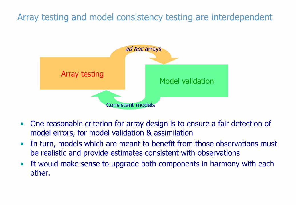
Array design

• Motivation

– Observational arrays are too often designed ignoring objective criteria

• Objective

– Set up a simple, quantitative criterion to quantify trade-offs & options in the design of observing systems & arrays

• Framework: integrated model/observations approach

– What does the model have to say about observations?

– What do observations have to say about the model?

– Use data assimilation theoretical framework

• Array design approaches in Toulouse group

– Regular OSSEs (e.g. Lamouroux et al., 2007, Jordà et al., 2007)

– EnKF-based ensemble variance reduction studies (e.g. Mourre et al., 2005; 2006; Ayoub et al., 2010)

– Stochastic Representer Matrix analysis (Le Hénaff et al., 2009; De Mey et al., 2010)

Applications by Charria, Lamouroux et al. (2011, 2013)

A simple problem

x augmented state vector (n,1) over time interval of interest

(let me insist on the fact that this is an augmented state vector – everything that will be

shown in this talk includes time as well as space in the definition of observations and

prior state estimate)

oy observations (p,1) verifying to H xy , with:

H( ) observation operator (not necessarily linear, but use linearized version)

),0( RN

Q: how can we characterize the performance of an array (H, R)?

Assume we have a prior state estimate of x and associated error statistics (if not, any

observational array will bring valuable information proportionately to its cost):

tfxx , with:

),0( fN P

What information does the array bring in?

Incremental information brought in by the observations (on top of prior):

Innovation vector Hxyyyd fogo H

The 2nd-order statistics of d can be used to characterize the amount of discrepancy

brought in by the observational array (on top of prior):

TfTHHPRdd , with:

TfHHP Representer matrix : prior state error covariance in observational space Tf

HP Matrix of representers : provide extrapolation from observational array

Representers contain information on how observations are able to detect prior state

error, and constrain an “optimal” solution through extrapolation:

- Extrapolation in space and time

- Extrapolation across variables (in particular the unobserved ones: multivariate

character)

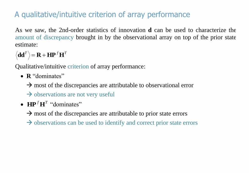
A qualitative/intuitive criterion of array performance

As we saw, the 2nd-order statistics of innovation d can be used to characterize the

amount of discrepancy brought in by the observational array on top of the prior state

estimate:

TfTHHPRdd

Qualitative/intuitive criterion of array performance:

R “dominates”

most of the discrepancies are attributable to observational error

observations are not very useful

TfHHP “dominates”

most of the discrepancies are attributable to prior state errors

observations can be used to identify and correct prior state errors

Towards a formal criterion of array performance

Two paths (among others) to formalize the intuitive order relationship…

Bennett’s “array modes” (e.g. Bennett et al., 1997): these are orthonormal rotation

vectors obtained by diagonalizing the representer matrix:

TTfβλβHHP

: observable degrees of freedom of the physical system for that configuration

: spectrum of RM, to be compared to the diagonal of R (obs. noise floor)

Le Hénaff & De Mey (Le Hénaff et al., 2009): in the general case of non-

homogeneous, non-diagonal R, and observational samples scattered in time, space, and

across variables, use spectrum and array modes of the scaled representer matrix : TTf

μσμRHHPRχ 2/12/1

: spectrum of SRM, to be compared to the diagonal of I (obs. noise floor)

Modal representers μRHPρ2/1 Tf

= representers for the array modes

Stochastic implementation of RM analysis

)2010.,(1

1

)..(:

2/1 aletSakovm

anomaliesEnsembleforecastgesamplesofMatrix

f

f

HARS

A

criterionoriginalofbasis

matrixofestimatem

ofestimatem

TT

TTff

fTfff

2/12/12/12/1

2/12/1

)()ˆ(

))((1

1ˆ

1

1ˆ

RISSRRIFRdd

χSSHARHARχ

PAAP

We now have the following stochastic estimates:

σ̂ = RM spectrum = squares of the singular values of S

μ̂ = Array Modes = singular vectors of S

Modal Representers = μASρ ˆ

1

1ˆ T

m

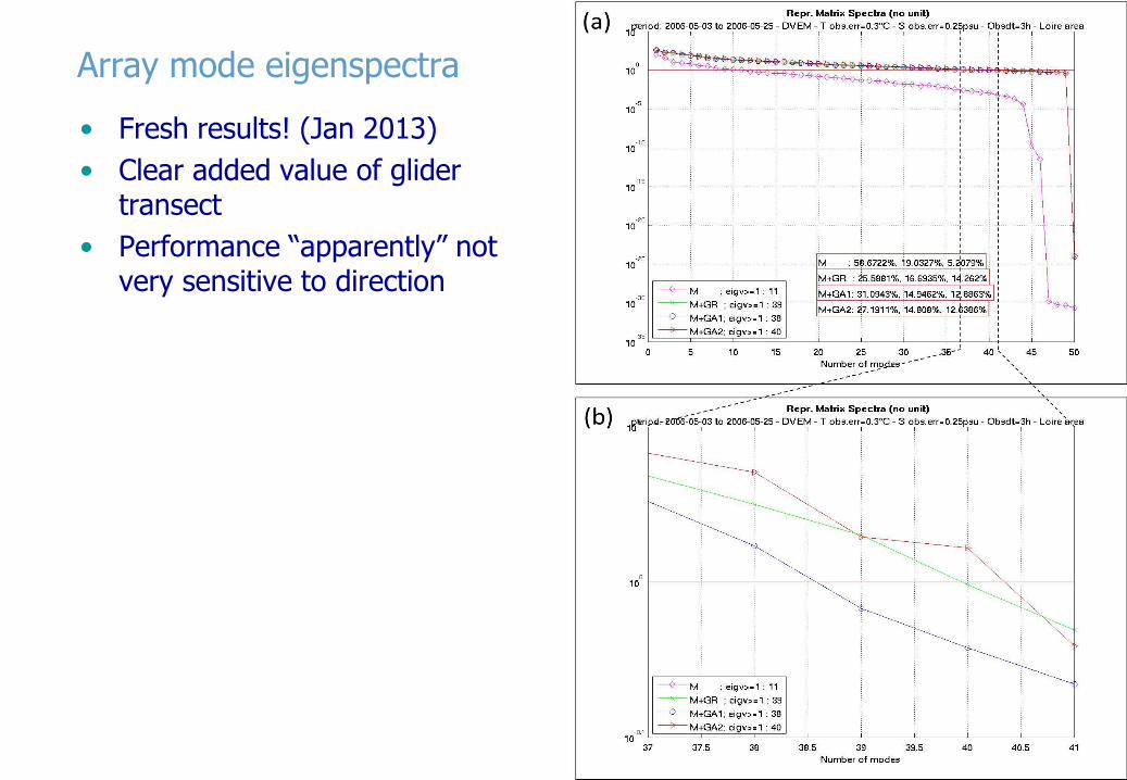
Stochastic RM spectrum analysis in practice

• RM analysis levels

– Eigenvalues above 1 are associated with array modes detectable above observational noise floor just count them

– Explore array modes & modal representers to get physical insight into the error subspace physical processes which are detectable (constrainable)

– Controllability cannot be checked (no DA)

• Origin of ensemble samples

– From stochastic modelling array performance results do not depend on DA

configuration and DA history

– From an Ensemble filter online analysis allow to study array performance

through regime changes, error estimates are typical of an assimilating system

• Assumptions on prior state error sources

– Comes back to prioritizing what the array is designed for

– E.g. wind stress, surface pressure, bathymetry, river runoff, turbulence (mesoscale, mixing), large-scale circulation, initial/boundary conditions, etc.

Mode 2: Meso1

Mode 3: Meso2+HF

A previous example: wide-swath vs. nadir altimeter

• Compare the performance of the JASON altimeter with the planned SWOT instrument (wide-swath altimetry)

• Only SWOT appears able to usefully detect & constrain coastal mesoscale patterns (array modes 2 and 3) and high-frequency events on the shelf (array mode 3)

RM spectra

JASON

SWOT

First 3 detectable array modes (SLA)

Le Hénaff & De Mey (LEGOS), 2008

4 1

SWOT vs. JASON-1 Mode 1: Swing

(common)

Bay of Biscay 3-km ensemble spanning stochastic response to

wind errors

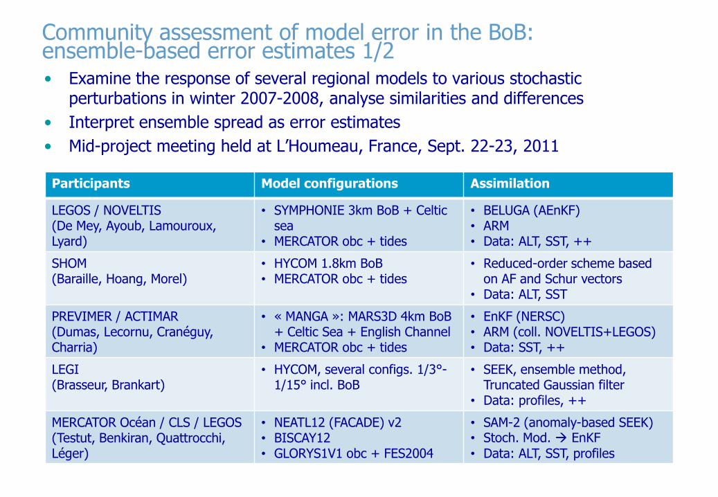
Community assessment of model error in the BoB: ensemble-based error estimates 1/2 • Examine the response of several regional models to various stochastic

perturbations in winter 2007-2008, analyse similarities and differences

• Interpret ensemble spread as error estimates

• Mid-project meeting held at L’Houmeau, France, Sept. 22-23, 2011

Participants Model configurations Assimilation

LEGOS / NOVELTIS (De Mey, Ayoub, Lamouroux, Lyard)

• SYMPHONIE 3km BoB + Celtic sea

• MERCATOR obc + tides

• BELUGA (AEnKF) • ARM • Data: ALT, SST, ++

SHOM (Baraille, Hoang, Morel)

• HYCOM 1.8km BoB • MERCATOR obc + tides

• Reduced-order scheme based on AF and Schur vectors

• Data: ALT, SST

PREVIMER / ACTIMAR (Dumas, Lecornu, Cranéguy, Charria)

• « MANGA »: MARS3D 4km BoB + Celtic Sea + English Channel

• MERCATOR obc + tides

• EnKF (NERSC) • ARM (coll. NOVELTIS+LEGOS) • Data: SST, ++

LEGI (Brasseur, Brankart)

• HYCOM, several configs. 1/3°-1/15° incl. BoB

• SEEK, ensemble method, Truncated Gaussian filter

• Data: profiles, ++

MERCATOR Océan / CLS / LEGOS (Testut, Benkiran, Quattrocchi, Léger)

• NEATL12 (FACADE) v2 • BISCAY12 • GLORYS1V1 obc + FES2004

• SAM-2 (anomaly-based SEEK) • Stoch. Mod. EnKF • Data: ALT, SST, profiles

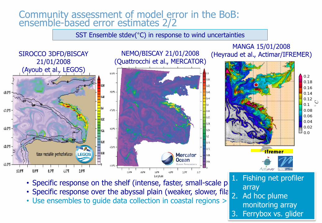
NEMO/BISCAY 21/01/2008 (Quattrocchi et al., MERCATOR)

SIROCCO 3DFD/BISCAY 21/01/2008

(Ayoub et al., LEGOS)

• Specific response on the shelf (intense, faster, small-scale patches) • Specific response over the abyssal plain (weaker, slower, filament-like) • Use ensembles to guide data collection in coastal regions >

Community assessment of model error in the BoB: ensemble-based error estimates 2/2

SST Ensemble stdev(°C) in response to wind uncertainties

MANGA 15/01/2008 (Heyraud et al., Actimar/IFREMER)

1. Fishing net profiler array

2. Ad hoc plume monitoring array

3. Ferrybox vs. glider

1. RECOPESCA fishing net array

• Vertical profilers on fishing nets – 3 scenarii: year 2008, year 2010, 2006-2011

• Observation error: 0.3°C

• Model uncertainty from MARS3D ensemble (50 members)

12

2008 reference SC1 : based on 2010 SC2 : cumulated 2006-2011

Charria (Ifremer), Lamouroux (Noveltis), De Mey (LEGOS) et al.

Ensemble generation (Craneguy/Heyraud/Raynaud, Actimar) • MeteoFrance atmospheric ensemble (U10, V10, T2m, Pmsl, Tcc) • Bottom friction coefficient Z0

• Extinction coefficient (impacts plumes) coext • Turbulent closure parameter Ck

Model uncertainties at observation positions (x,y,z,t)

Array mode eigenspectra

• Rank-limited

• Larger number of observations (SC2) = errors better sampled

• Geographical spread more important than number of profiles: REF more efficient than SC1

Array ev>1 Profiles Ratio

REF 29 126 0.23

SC1 48 265 0.18

SC2 >49 843 >0.05

GR

GA1

GA2

M

2. What is the best glider section to monitor the structure of the Loire river plume and its time evolution?

• A minimal network (based on prospective work): 1 mooring + 1 glider

• Observation error: 0.3°C / 0.25psu

• Model uncertainty from MARS3D ensemble (50 members)

Charria (Ifremer), Lamouroux (Noveltis), De Mey (LEGOS) et al.

How the array “sees” the salinity & salinity error

Array mode eigenspectra

• Fresh results! (Jan 2013)

• Clear added value of glider transect

• Performance “apparently” not very sensitive to direction

Modal representers – Salinity

• Glider section brings in finer detail

• Polarization effect

3. Roscoff-Plymouth Ferrybox vs. Glider

• Even fresher results

• Higher repeat cycle of ferrybox critical here, despite being surface only, because of HF model errors (linked to tidal front displacements)

Charria (Ifremer), Lamouroux (Noveltis), De Mey (LEGOS) et al.

Role of this approach in a coastal array strategy?

• Example of Ifremer

– Exchanges and technology improvements through European projects (FP7

JERICO in progress, future NEXOS FP7 proposal) – including stochastic RM

analysis and OSE/OSSE to quantify the added value for modelling systems

– End of PREVIMER project in October 2013… follow-up possibly based on

regional (CPER) projects for observation networks: submitted early proposal for

observation network around Brittany – including design of observation network

based on stochastic RM analysis

• In general

– High potential for projects or agencies structured beyond the old provider/user

data model (e.g. coastal observatories, IOOS-type programs)

Conclusions

• Integrated model/observations approach

– Some coastal groups are structured beyond the old provider/user data model (e.g. some coastal observatories, IOOS-type programs)

– What does the model have to say about observations?

– What do observations have to say about the model?

• Stochastic RM analysis is a useful tool for array testing based on the detection of prior errors

– Approach provides a way to prioritize array options given a library of ensemble members

– Impact analysis can be performed on unobserved variables via modal representers

– Complementary with other existing array design approaches: OSSEs, targeted observations, etc.

• Approach requires realistic estimates of model uncertainties

– Physical insight needed into error processes, in order to make sure that the right d.o.f.’s are open

– Methods to validate ensembles needed.

Array testing and model consistency testing are interdependent

• One reasonable criterion for array design is to ensure a fair detection of model errors, for model validation & assimilation

• In turn, models which are meant to benefit from those observations must be realistic and provide estimates consistent with observations

• It would make sense to upgrade both components in harmony with each other.

Array testing Model validation

ad hoc arrays

Consistent models

We are willing to collaborate with interested groups!