HAL Id: tel-01126901 https://tel.archives-ouvertes.fr/tel-01126901 Submitted on 6 Mar 2015 HAL is a multi-disciplinary open access archive for the deposit and dissemination of sci- entific research documents, whether they are pub- lished or not. The documents may come from teaching and research institutions in France or abroad, or from public or private research centers. L’archive ouverte pluridisciplinaire HAL, est destinée au dépôt et à la diffusion de documents scientifiques de niveau recherche, publiés ou non, émanant des établissements d’enseignement et de recherche français ou étrangers, des laboratoires publics ou privés. Goodness-of-fit tests in reliability : Weibull distribution and imperfect maintenance models Meryam Krit To cite this version: Meryam Krit. Goodness-of-fit tests in reliability : Weibull distribution and imperfect mainte- nance models. General Mathematics [math.GM]. Université de Grenoble, 2014. English. NNT : 2014GRENM038. tel-01126901
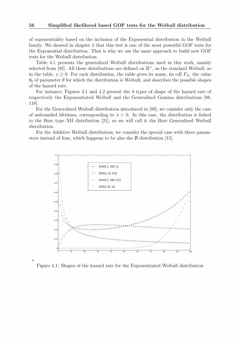
Transcript
HAL Id: tel-01126901https://tel.archives-ouvertes.fr/tel-01126901
Submitted on 6 Mar 2015
HAL is a multi-disciplinary open accessarchive for the deposit and dissemination of sci-entific research documents, whether they are pub-lished or not. The documents may come fromteaching and research institutions in France orabroad, or from public or private research centers.
L’archive ouverte pluridisciplinaire HAL, estdestinée au dépôt et à la diffusion de documentsscientifiques de niveau recherche, publiés ou non,émanant des établissements d’enseignement et derecherche français ou étrangers, des laboratoirespublics ou privés.
Goodness-of-fit tests in reliability : Weibull distributionand imperfect maintenance models
Meryam Krit
To cite this version:Meryam Krit. Goodness-of-fit tests in reliability : Weibull distribution and imperfect mainte-nance models. General Mathematics [math.GM]. Université de Grenoble, 2014. English. NNT :2014GRENM038. tel-01126901
DOCTEUR DE L’UNIVERSITE DE GRENOBLESpecialite : Mathematiques Appliquees
Arrete ministeriel : 7 aout 2006
Presentee par
Meryam Krit
These dirigee par Olivier Gaudoinet codirigee par Laurent Doyen et Emmanuel Remy
preparee au sein du Laboratoire Jean Kuntzmannet de de l’Ecole Doctorale Mathematiques, Sciences et Technologiesde l’Information, Informatique
Goodness-of-fit tests in reliability:Weibull distribution and imperfectmaintenance models.
These soutenue publiquement le 16 octobre 2014,devant le jury compose de :
M. Laurent BordesProfesseur a l’Universite de Pau et des Pays de l’Adour, RapporteurM. Bo Henry LindqvistProfesseur a Norwegian University of Science and Technology, Trondheim,Norvege, RapporteurM. Jean-Yves DauxoisProfesseur a l’INSA de Toulouse, ExaminateurM. Olivier GaudoinProfesseur a Grenoble INP - Ensimag, Directeur de theseM. Laurent DoyenMaıtre de conferences a l’Universite Pierre Mendes France, Co-Directeur detheseM. Emmanuel RemyIngenieur chercheur expert a EDF R&D, Co-Directeur de these
3
Remerciements
Entre un melange de sentiment de deuil et de culpabilite. Je souhaite dedier ma these ama tante Rkia que j’ai perdue quelques jours avant ma soutenance sans que ma famille etmoi ne le sachions. Elle voulait que je lui envoie mon manuscrit de these, elle se sentaitcapable de le lire et de le comprendre s’il etait en francais!
Elle n’arretait pas de nous faire rire avec ses blagues. Je me souviens encore de notredernier fou rire car elle adorait coudre des poches a ses robes a partir des manches. Ellenous a beaucoup seduit par sa generosite voire son altruisme ... Donner sans attendre enretour. Je pense a ses dons pour les gens dans le besoin, ses petites balades et ses cadeauxaux jeunes adolescents defavorises.
Je pense a toute ma famille malgre ma colere contre eux d’avoir attendu pour nousannoncer la triste nouvelle. Je pense a mon cousin Adnane, ses petits enfants Nour etKhalid, mes tantes Mellouki, Souad et Fatima, mes oncles Simo et Boubker, mes cousinesSalma et Mouna et a ma mere. Je tiens a leur exprimer tout mon soutien et mon amour.
Je tiens a remercier mon directeur de these Olivier Gaudoin pour tout son soutien etson attention depuis mes premiers cours de statistiques a l’Ensimag, ses encouragementspendant la these et meme apres la these. Mais aussi pour la qualite de son encadrementet surtout sa gentillesse et son ouverture d’esprit. Je remercie aussi mes deux encadrantsLaurent Doyen et Emmanuel Remy pour leurs relectures minutieuses et leur encadrementpendant ces trois ans de these.
Laurent Bordes et Bo Lindqvist m’ont fait l’honneur d’etre rapporteurs de ma theseet ont pris le temps de se deplacer. Pour tout cela je les remercie. Je remercie egalementJean-Yves Dauxois pour avoir accepte de presider mon jury.
Mes remerciements vont aussi a tous les thesards du LJK : Ester, Gildas, Chris-tine, Jonathon, Farida, Kevin, Nadia, Federico, Amine, Matthias, Pierre Olivier, Chloe,Meryem, Nelson, Roland, Margaux, Morgane, Pierre Jean, Nhu. Je remercie Anne etLaurence de leur gentillesse.
Je remercie specialement, Maha Moussa pour sa generosite, sa gentillesse et son amourinfini, merci pour le pot et la decoration.
Il m’est impossible d’oublier toute la communaute libanaise de Grenoble : Roland,Makieh, Rida, Ali, Hassan, Sandra, Hind, Mahmoud, Wael, Jihad, Hassan et Sara Bazzi.J’adresse mes sinceres remerciements a l’adorable Wafa pour sa presence et son soutiencontinu et a Jeremy pour nos debats sur les questions existentielles qui ne finissent jamais.Je remercie egalement mes copines Leyla, Siham et Aliae qui sont comme des soeurspour moi. Merci de m’avoir toujours soutenu avant et pendant la these, d’avoir fait ledeplacement de Paris pour ma soutenance et pour votre attention sans fin.
Je souhaite aussi remercier certaines personnes qui ont beaucoup marque ma vie.Malgre la distance je pense a eux : Chourouk, Keiko, Oum lfadl, Karn, Leyla-san, Jihene,Nada, la famille Sahil specialement Wafa Sahil et sa maman Latifa pour leur accueil aAgadir et leur generosite, la famille Bami particulierement Nabila et sa maman Leyla. Jeremercie aussi la famille El Bahri pour leur accueil a Grenoble, la famille Francon pourleur gentillesse et leur accueil chez eux a Montelimar.
4
Je tiens a remercier particulierement tout le departement MRI d’EDF R&D pourleur accueil et pour les conditions de travail privilegiees qui m’ont ete offertes et tousles thesards, en premier mes co-bureaux Jean-Baptiste et Guillaume et aussi Jeanne etVincent.
Je voudrais egalement remercier ma deuxieme famille de France, la famille des cham-pions Calandreau pour leur soutien continu. Je remercie Steph, Emeric, Benix, Julietteet mes parents de France Alain et Veronique. Je sais que je dois m’entraıner dur pourfaire les cross avec vous et pas seulement venir encourager. On aura encore pleins decompetitions, de tours du lac et de voironnaises a organiser ... sans courir!
Mes plus profonds remerciements vont a mes parents qui m’ont toujours soutenu etencourage pendant mon cursus scolaire et je les remercie de nous avoir donne (mes soeurs,mon frere et moi) toutes les chances pour reussir. La these n’est qu’un aboutissement deleurs efforts, leur devouement et leur amour infini. J’en profite pour leur exprimer maplus grande gratitude.
Une pensee pour ma grand-mere qui j’espere sera fiere de moi la ou elle est, meme sije ne suis pas devenue ministre d’industrie du Maroc et que je ne sais pas encore cuisinercomme elle l’esperait. Je remercie egalement mon frere Badr, ma belle-sœur Nawal et messœurs Bouchra, Sara et Kawtar de me faire rire tout les jours avec leurs messages pleinsd’humour et d’amour.
ABAO As Bad As OldAGAN As Good As NewARA1 Arithmetic Reduction of Age model with memory oneARA∞ Arithmetic Reduction of Age model with infinite memoryBFGS Broyden-Fletcher-Goldfarb-Shanno algorithmBP Brown-Proschan modelBPl Brown-Proschan model with log-linear failure intensityBPp Brown-Proschan model with power-law failure intensityBT bathtub shaped hazard ratecdf cumulative distribution functionCM corrective maintenanceDHR decreasing hazard rateGOF goodness-of-fitGRA Geometric Reduction of AgeHPP Homogeneous Poisson ProcessIHR increasing hazard rateiid independent and identically distributedLLP log-linear processLSE least squared estimatorME moment estimatorMLE maximum likelihood estimatorNHPP Non Homogeneous Poisson Processpdf probability density functionPLP power-law processPM preventive maintenanceRP renewal processUBT upside-down bathtub shaped hazard rate
10 CONTENTS
Chapter 1
Introduction
1.1 Industrial context
Risk management of industrial facilities, such as EDF power plants, needs to accuratelyassess and predict systems reliability. Depending on the available knowledge, three maintypes of approaches are commonly used to assess systems reliability. If operation feedbackdata is available, the classical frequentist statistical approach can be used. When theoperation feedback data is not informative enough, the Bayesian statistical approach isa convenient alternative since it allows adding knowledge from expert judgment [51].When the systems failure has never been observed during the operation time period, astructural reliability analysis can be carried out to assess risk indicators from numericalmodels representing the physical behavior of the systems [86, 32].
In this dissertation, one considers the situation where operation feedback data is avail-able and is the only source of knowledge about the systems reliability: thus the classicalfrequentist statistical approach is our scope of work. Sometimes one can obtain usefulresults using non parametric techniques that do not require any choice of a probabilisticmodel. It is the case for instance when estimating a Mean Time to Failure (MTTF) bythe mean value of the observed operation lifetimes of the systems that failed. But, ifone is able to choose an appropriate probabilistic parametric model, this presents severaladvantages:
• the hypothesis of the model may allow to better understand the nature of the randomobserved phenomenon
• the estimation of the reliability indicators is of a better quality
• an adapted model allows to make predictions outside the operation feedback dataset which can not be accomplished by a non parametric method.
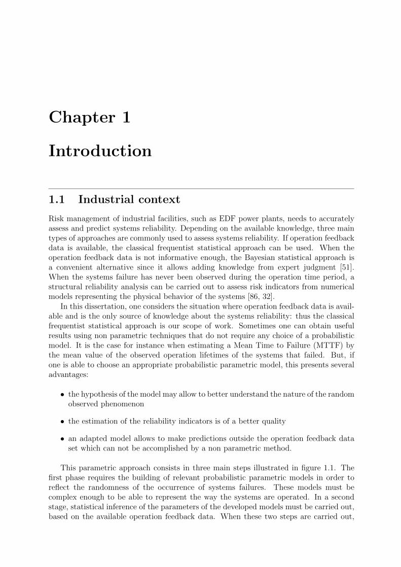
This parametric approach consists in three main steps illustrated in figure 1.1. Thefirst phase requires the building of relevant probabilistic parametric models in order toreflect the randomness of the occurrence of systems failures. These models must becomplex enough to be able to represent the way the systems are operated. In a secondstage, statistical inference of the parameters of the developed models must be carried out,based on the available operation feedback data. When these two steps are carried out,
12 Introduction
a final stage, as important as the previous ones, consists in firstly validating the fittedmodels using statistical criteria and secondly comparing the different competing models.The subject of the PhD thesis falls within this last stage of model validation and selection,which is a crucial issue.
Figure 1.1: Three main steps of the approach
Indeed from a regulatory point of view, electric utilities have to present convincingquantitative arguments to regulatory authorities in order to justify systems reliability.It is thus essential to ensure the fitted models are relevant (even the best) given theoperation feedback data. From a performance point of view, the misspecification of thesystems reliability models can lead to establish inappropriate preventive maintenanceplans resulting in poor availability and economic performance of the power plants.
That is why it is crucial for EDF to have efficient probabilistic and statistical tech-niques to determine the closest reliability models to the reality and prove their relevanceand quality.
1.2 Operation feedback data and reliability models
Depending on the characteristics of the studied systems, specific operation feedback dataare observed and appropriate probabilistic reliability models must be used to representreal-life condition. The simplest case is the one of non repairable systems, generallycomponents. The quantity of interest is the operation time before the (unique) failure ofthe systems. The feedback data from the operation of a fleet of components is made of:
• complete data associated with the operation times of the components that failed;
Introduction 13
• censored data relative, for instance, to the lifetimes of the components that did notbreak down during the operation time period.
When the components are identical (from design, manufacturing, operation, mainte-nance, environmental ... points of view) and independent (no common cause failures), theoperation feedback data is thus compounded of observations which constitute a sampleof independent random variables following the same distribution (identically distributed).For instance, table 1.1 presents a classical data set of the literature [2]. It gives the failuretimes of 50 devices.
Table 1.1: Failure data of 50 devices (Aarset data)
The most usual distribution used to represent the lifetime of components are theExponential and the Weibull distributions. These distributions are widely used to modelthe lifetimes of non repairable systems. The Exponential distribution represents thedisadvantage of having a constant failure rate. The Weibull distribution is a more flexiblemodel since it allows decreasing, constant and increasing failure rates. It is then essentialto be able to check the relevance of these two distributions for a given data set. In thiswork, we focus on the two-parameter Weibull distribution.
It is important to highlight that even if the Weibull distribution is popular in relia-bility survival and analysis, it is also frequently used in many other technical fields: onecan mention environmental sciences (weather forecasting and hydrology), insurance, ge-ology, chemistry, physics, medicine, economics and geography. Due to its close link to theextreme value distribution, the Weibull model also appears in the extreme value theory.Last but not least, the founding work of Waloddi Weibull [128] in the field of structuralmechanics stresses the relevance of using the Weibull distribution to model physical pa-rameters such as the mechanical toughness (or strength) of a material and the length ofdefects. EDF is also interested by data of that kind. For instance, table 1.2 presentsmeasures of toughness of EDF material at a specific temperature δ2. These data havebeen modified for confidentiality reasons.
The case of repairable systems is more complex. Firstly let us suppose no preventivemaintenance (PM) is carried out on the system (the ”run to failure” strategy is adopted).
14 Introduction
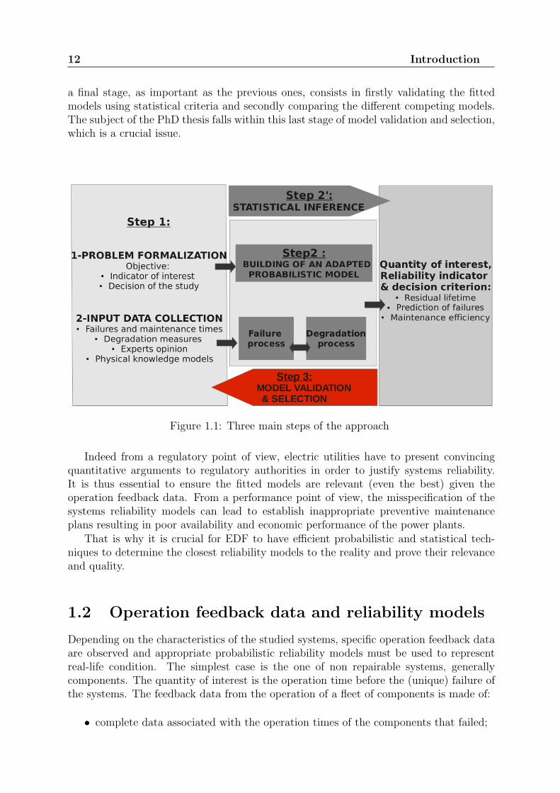
After a failure, a repair (or corrective maintenance - CM) is carried out so that the systemcan perform its function again. Throughout the thesis, we will consider that repair timesare negligible or not taken into account, so failure times and CM times are identical. Fora given piece of equipment, one is interested in the time sequence of the successive CM.It is a sequence of recurrent events which can be modeled by a univariate point process.Figure 1.2 illustrates the occurrence of CM for a repairable system. Table 1.3 representsCM times (in days) of some type of pipes within the boiler of an EDF coal-fired powerstation. The welds of the straps holding these pipes are subjected to corrosion leadingto the initiation then propagation of flaws that may endanger the stability of the pipes.Since it has no major impact on the operation of the plant, a run to failure maintenanceplan is carried out.
Figure 1.2: Occurrence of CM of a repairable system
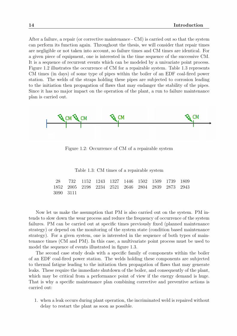
Now let us make the assumption that PM is also carried out on the system. PM in-tends to slow down the wear process and reduce the frequency of occurrence of the systemfailures. PM can be carried out at specific times previously fixed (planned maintenancestrategy) or depend on the monitoring of the system state (condition based maintenancestrategy). For a given system, one is interested in the sequence of both types of main-tenance times (CM and PM). In this case, a multivariate point process must be used tomodel the sequence of events illustrated in figure 1.3.
The second case study deals with a specific family of components within the boilerof an EDF coal-fired power station. The welds holding these components are subjectedto thermal fatigue leading to the initiation then propagation of flaws that may generateleaks. These require the immediate shutdown of the boiler, and consequently of the plant,which may be critical from a performance point of view if the energy demand is huge.That is why a specific maintenance plan combining corrective and preventive actions iscarried out:
1. when a leak occurs during plant operation, the incriminated weld is repaired withoutdelay to restart the plant as soon as possible.
Introduction 15
2. scheduled preventive inspections of the hazard zones of the system are carried outperiodically and the detected cracks are scoured.
Table 1.4 gives the PM and CM times of these welds [35].
Figure 1.3: Occurrence of CM and PM of a repairable system
Table 1.4: CM and PM times of a repairable system
25 50 93 109 114 141 163 164 195 225 264PM CM CM CM PM CM CM CM CM PM PM
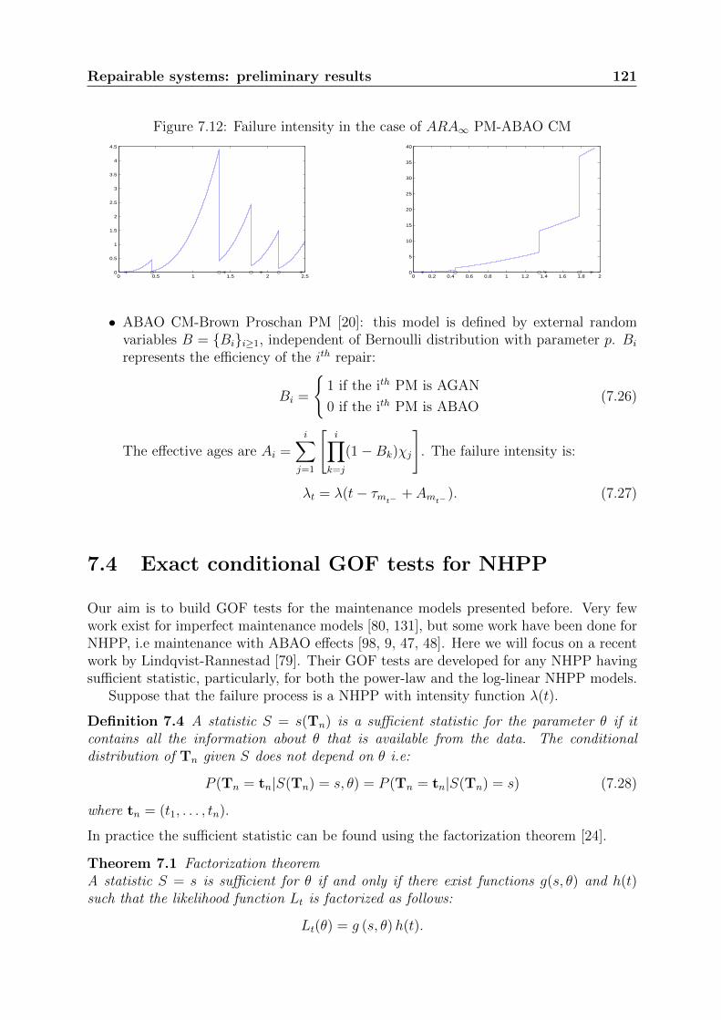
For maintained systems, the maintenance effect naturally impacts the system relia-bility. A first classical approach to take into account this impact is to assume that themaintenance is minimal, which means it leaves the system in the same state as it wasjust before. It characterizes a maintenance effect that neither improves nor damages thesystem. It is called As Bad As Old (ABAO) maintenance and the corresponding ran-dom process family is the Non Homogeneous Poisson Processes (NHPP). A second basichypothesis consists in assuming that the maintenance is perfect, which means that it per-fectly repairs the system and leaves it as if it was new. The latter is ”As Good As New”(AGAN) after maintenance and the system is comparable to a similar new system putinto operation just after the previous maintenance. The corresponding random processfamily is the renewal processes. Obviously standard maintenance reduces failure inten-sity but does not systematically leave the system as good as new: reality is between thetwo extreme cases previously presented. In the literature, models enabling to take intoaccount a maintenance effect between ABAO and AGAN are known as imperfect main-tenance models. Many models have been suggested [63, 20] and among them the mostpopular are the virtual age models, for which the maintenance rejuvenates the system[63]. The Arithmetic Reduction of Age (ARA) models are one of those and are based onan arithmetic reduction of what is called the virtual age of the system [33, 34, 35].
In order to take into account the diversity of the types of systems which are installedwithin EDF power plants, it is necessary to have validation and selection statistical indi-cators adapted for the different probabilistic models which have just been presented.
1.3 Goodness-of-fit tests
As already mentioned, it is fundamental to be able to choose an adapted parametric modelto a given data set and choose the best fitted model from a large range of candidate models.
16 Introduction
It is a classical statistical issue known as model validation and selection. Goodness-of-fit(GOF) tests are a useful tool to achieve this goal.
There is a wide literature on GOF tests for the Exponential distribution, but very littleattention was paid to GOF tests for parametric models suitable in the field of industrialreliability, such as the Weibull distribution and the imperfect maintenance models thathave been presented in the previous section.
Moreover, in nuclear electricity generation industry, systems failures are rare events,leading to small and highly censored data sets which make the use of standard statisticaltechniques difficult (even impossible). That is why the subject of the thesis, “GOF testsin reliability: Weibull distribution and imperfect maintenance models”, is as challengingas the imposed industrial constraints which require the development of new methods.
The first aim of the dissertation is to develop GOF tests for basic models like samplesof independent and identically distributed (iid) random variables, in order to answer thequestion whether an iid sample comes from a specific distribution (the Exponential or theWeibull distributions) or not. The second aim answers the same question for more so-phisticated models: Non Homogeneous Poisson processes (NHPP), imperfect maintenancemodels, ...
For non-repairable systems, we consider n similar systems operating independentlyto each others. Their lifetimes are considered to be realizations of random variablesX1, . . . , Xn independent and identically distributed.
If all the lifetimes of the n systems are observed, they constitute a complete sample.When not all the lifetimes are observed, it is a censored sample. There exist several kindsof censoring: left or right, type I or type II, simple or multiple, etc ...
For non-repairable systems, we will be interested basically in complete samples andin some cases simple type II censored samples. Type II left-censoring occurs when thesmallest s lifetimes are not observed and type II right-censoring occurs when the largestr lifetimes are not not observed.
For repairable systems, we consider that we are studying one system that can besubject to CM or PM. The quantities of interest are the CM times of the given system.The PM are considered to be deterministic. The CM are considered to be the realizationsof a random point process. The question is still to find the best fitted point process tomodel the occurrence of the failures. The system is assumed to be repaired after eachfailure so we consider in all the studied cases that we have type I right-censoring whichmeans the observation stops after a given censoring time T .
The example of data in table 1.1 presents realizations of iid random variables. Theproblem of interest is to find a model which fits well this data set. The problem is expressedas a statistical test. We denote F the unknown distribution function of the sample.This distribution is assumed to be continuous. In the case of discrete distributions, thepresented procedures need some arrangements that are not always simple. The GOF testsfor discrete distribution are detailed in chapter 7 of [18].
We distinguish two cases, depending on whether we want to test the goodness-of-fitto an entirely specified distribution or to a family of distributions.
• GOF tests to an entirely specified distribution:
H0 : “F = F0” vs H1 : “F 6= F0”. (1.1)
Introduction 17
• GOF tests to a family of distributions:
H0 : “F ∈ F” vs H1 : “F /∈ F”. (1.2)
Often, family F is a parametric family: F = F (.; θ); θ ∈ Θ. It is the case when wetest whether the Aarset data comes from a Weibull distribution without precising specificvalues of the parameters. If a Weibull distribution is adapted, we can estimate lately itsparameters.
The examples in tables 1.3 and 1.4 give CM and PM times of a repairable system. Theobservations in this case are realizations of a point process. We want to find a relevantmodel for this process. We denote λ. the unknown intensity function of the point process.The GOF test in this case has the following hypotheses:
H0: “λ ∈ I” vs H1 : “λ /∈ I”
where the family I is a parametric family: I = λ(.; θ); θ ∈ Θ. For instance, one maywant to test a NHPP with a specific intensity function, either a power law intensity or aNHPP with log-linear intensity function.
1.4 Structure of the dissertation
The thesis is structured in two parts of unequal size. Chapters 2 to 6 are devoted to non-repairable systems and Chapters 7 and 8 to repairable systems. Two appendices providetables of results and a documentation of the R package EWGoF we have developed.
Chapter 2 presents a review of existing GOF tests for the Exponential distribution,for complete and censored samples. A comprehensive comparison study is done, usingMonte-Carlo simulations. It leads to identify the best of these tests.
Chapter 3 is the first of 4 chapters dedicated to the two-parameter Weibull distribution.First it gives the definitions and main properties of this distribution, that will be usedthroughout the dissertation. Then, it presents a review of existing GOF tests for theWeibull distribution.
In Chapters 4 and 5, we propose two new families of GOF tests for the Weibull dis-tribution. Chapter 4 is dedicated to likelihood-based tests. These tests consist in nestingthe two-parameter Weibull distribution in three-parameter generalized Weibull familiesand testing the value of the third parameter by using the Wald, score and likelihoodratio procedures. We simplify the usual likelihood based tests by getting rid of the nui-sance parameters, using three estimation methods, maximum likelihood, least squares andmoments.
Chapter 5 presents a second new family of GOF tests for the Weibull distribution,based on the Laplace transform. These tests merge the ideas of Cabana and Quiroz [22]and those introduced by Henze [53] for testing the Exponential distribution. We alsointroduce new versions of the statistics of Cabana and Quiroz, using maximum likelihoodestimators instead of moment estimators.
Chapter 6 presents a comprehensive comparison study of all GOF tests for the Weibulldistribution. This comparison includes the usual GOF tests presented in Chapter 3 andthe new ones developed in Chapters 4 and 5. The idea of combining GOF tests is also
18 Introduction
introduced. Recommendations about the most powerful tests are given, according to thecharacteristics of the tested data. The best tests that we have identified are little knownand rarely used.
In Chapter 7, we move to the repairable systems case. This chapter gives some prelimi-nary results about nonhomogeneous Poisson processes and imperfect maintenance models,when both corrective and preventive maintenances are performed. The tests proposed byLindqvist and Rannestad [79] for testing the fit of NHPPs are presented. They are basedon conditional sampling given a sufficient statistic.
Chapter 8 is a first attempt to building GOF tests for imperfect maintenance models.The considered model assumes that the corrective maintenances are minimal (ABAO)with a log-linear initial intensity. It also assumes that the preventive maintenances aredone at deterministic times and that their effect is of the Arithmetic Reduction of Agewith memory one (ARA1) type. In this case, a sufficient statistic exists and the tests ofLindqvist and Rannestad [79] can be generalized.
Chapter 9 presents the application of this study to real data sets, some from the liter-ature and some from EDF. These data sets are from both non repairable and repairablesystems. The practical use of the tests in an industrial context is detailed.
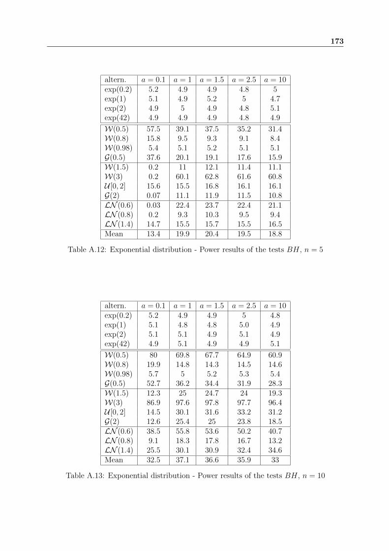
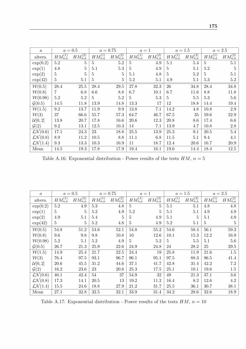
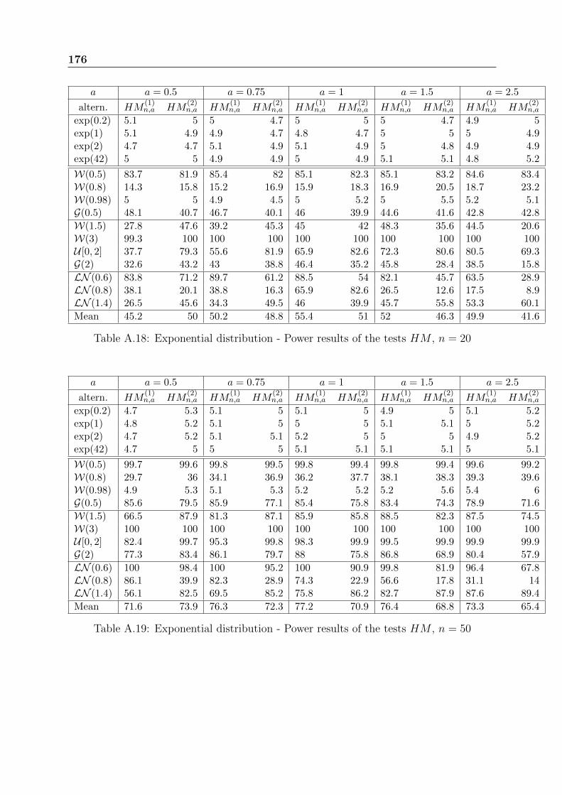
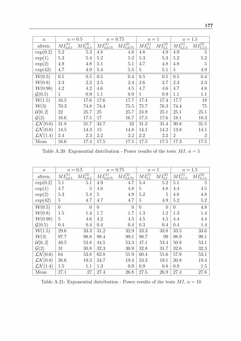
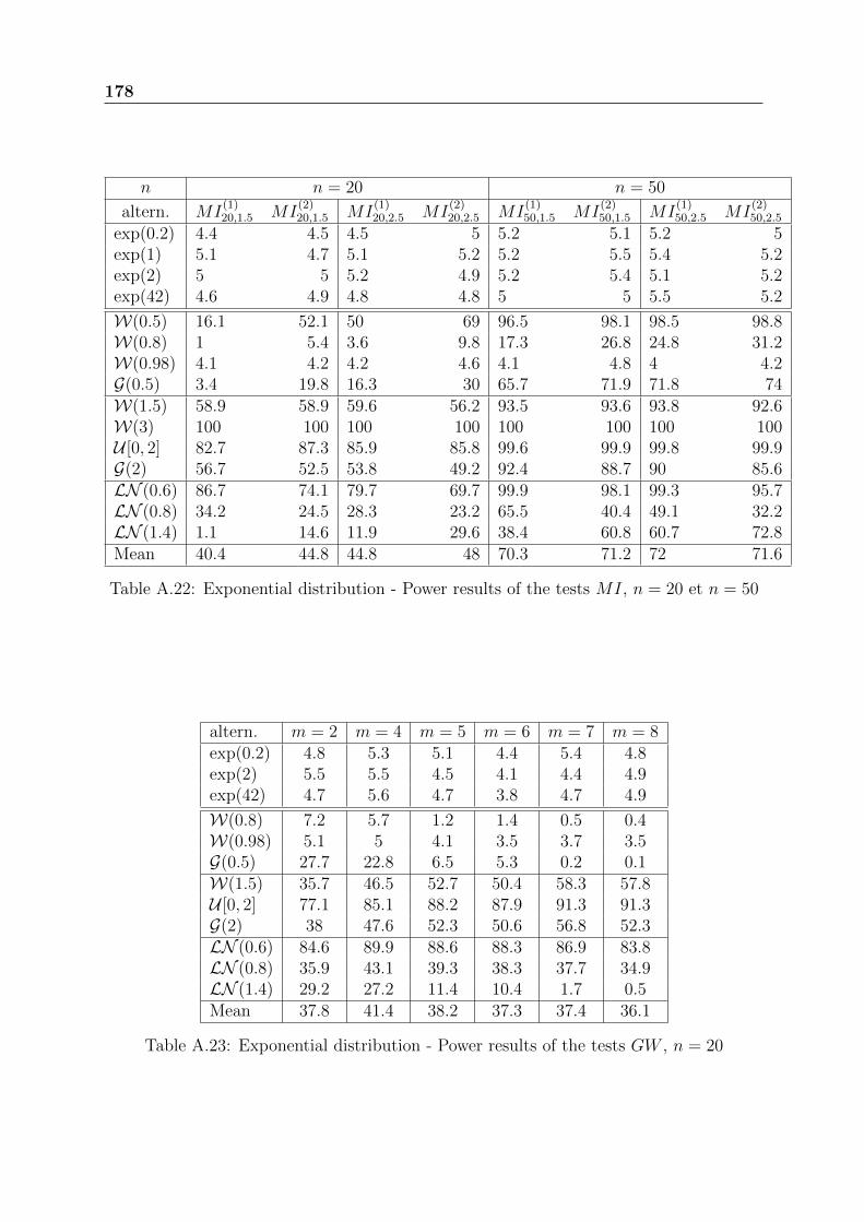
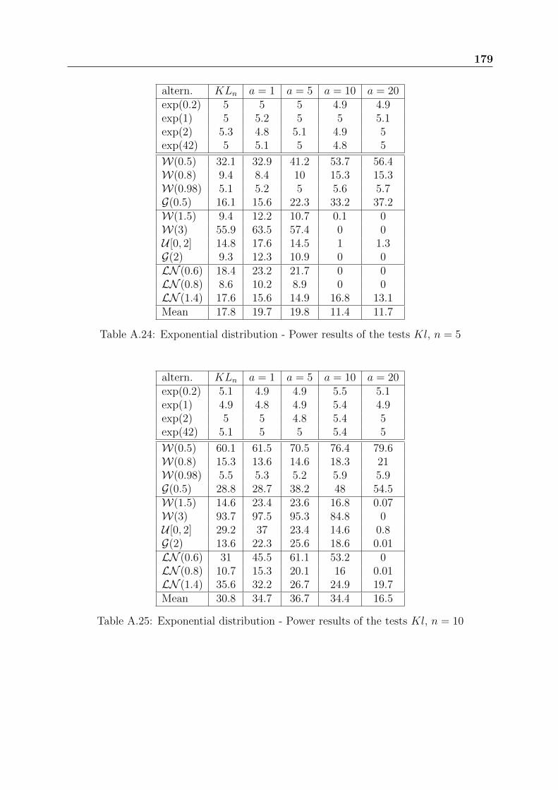
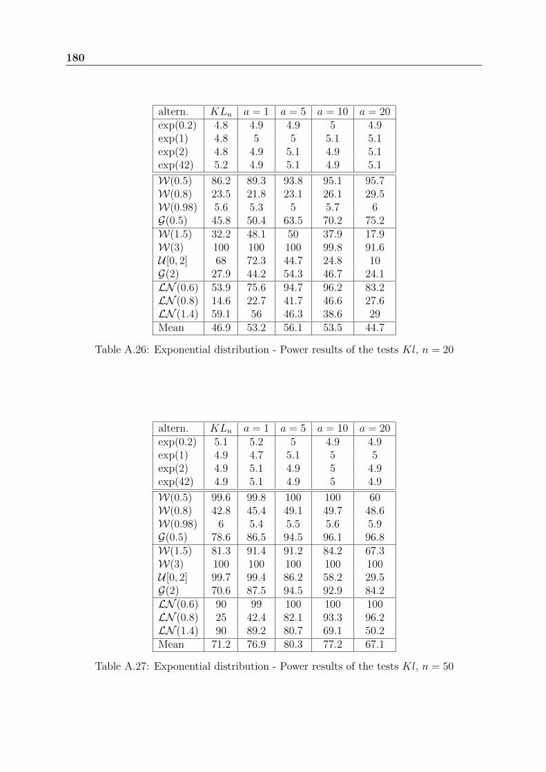
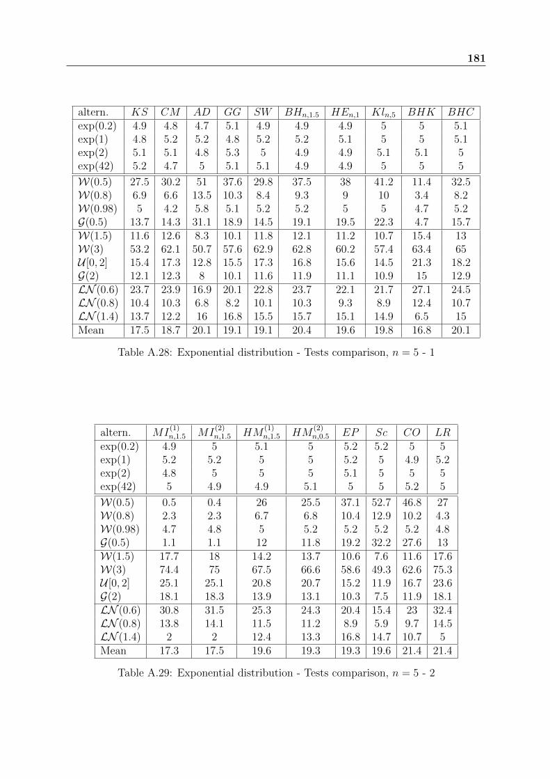
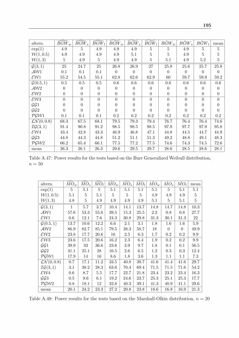
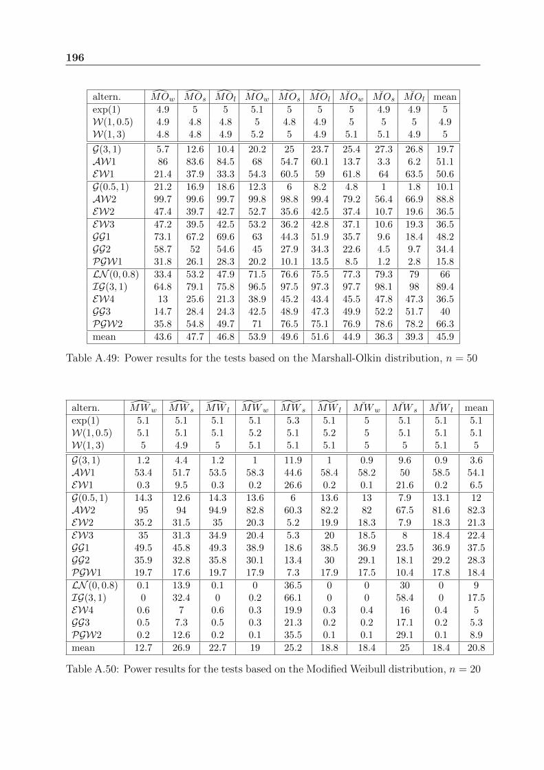
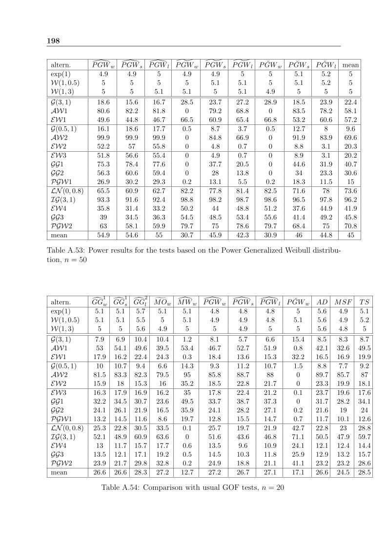
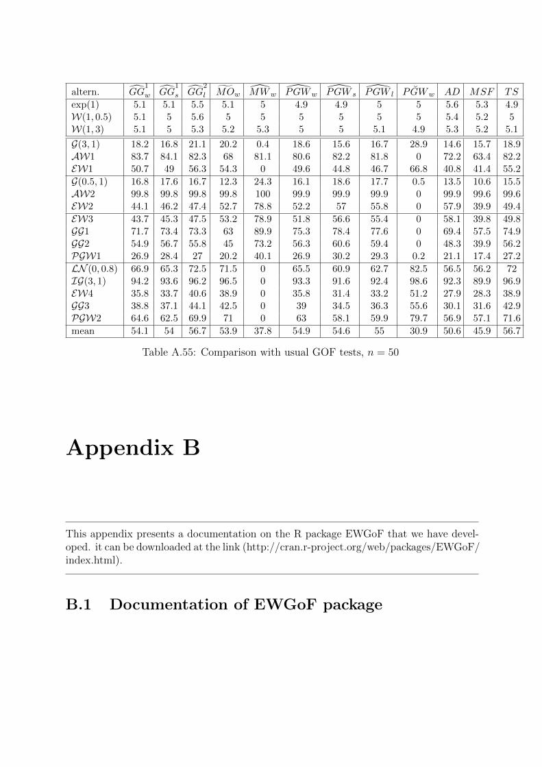
Appendix A contains a huge number of simulation results, which aim to assess thepower of GOF tests for the Exponential and Weibull distributions.
Appendix B gives a detailed documentation on the R package EWGoF that we havedeveloped. This package implements all the GOF tests for non repairable systems pre-sented in this dissertation: GOF tests for the Exponential distribution of Chapter 2 andGOF tests for the Weibull distribution of Chapters 3, 4 and 5. An important feature ofthese tests is that they are all exact: the critical values needed for performing the testsare obtained by Monte-Carlo simulation and no asymptotic results are used. Then, theGOF tests can be applied for any sample size. All the simulation results and applicationsto real data presented in the thesis have been done using the EWGoF package.
Chapter 2
Exponential distribution: basicproperties and usual GOF tests
This chapter is dedicated to the Exponential distribution. First, some definitions andbasic properties of this distribution are given. Then, we present a quick review of GOFtests for the Exponential distribution, based on different approaches: probability plots,empirical distribution function, normalized spacings, Laplace transform, characteristicfunction, entropy, integrated distribution function, likelihood based tests, ... Completeand censored samples are treated. Finally, an extensive comparison study is done whichleads to identify the best GOF tests for the Exponential distribution.
2.1 The Exponential distribution: definition and prop-
erties
A random variable X is from the Exponential distribution of parameter λ, denoted exp(λ),if and only if its cumulative distribution function (cdf) is:
F (x;λ) = 1− exp(−λx), x ≥ 0, λ > 0. (2.1)
• The probability density function (pdf) is:
f(x;λ) = λ exp(−λx), x ≥ 0, λ > 0. (2.2)
• The reliability is R(x) = 1− F (x, λ) = exp(−λx).
• The expectation (or the Mean time to failure MTTF) is: MTTF = E[X] =1
λ.
• The variance is V ar[X] =1
λ2.
20 Exponential distribution: basic properties and usual GOF tests
• The hazard rate is h(x) =f(x)
R(x)=λ exp(−λx)
exp(−λx)= λ.
• The mean residual life is m(x) = E[X − x|X > x] =1
λ= E[X].
• The Laplace transform is ψ(t) = E [exp(−tX)] =λ
λ+ t.
• The characteristic function is ϕ(t) = E [exp(itX)] =λ
λ− it .
• If X is from exp(λ), Y = λX follows a standard Exponential distribution exp(1).
The Exponential distribution is without memory. It means if that the system didnot fail yet at time t, then it behaves as if it was new at this time. Indeed, the randomvariable X obeys the following relation:
∀x ≥ 0, P (X > t+ x | X > t) = P (X > x). (2.3)
In reliability, it means that the Exponential distribution is suitable for systems which arenot deteriorating neither improving with time.
Let x1, . . . , xn be realizations of independent and identically distributed (iid) randomvariables X1, . . . , Xn with the exp(λ) distribution. The likelihood function is :
L(λ;x1, . . . , xn) =n∏
i=1
f(xi) = λn exp
(−λ
n∑
i=1
xi
). (2.4)
Maximizing this function, we obtain that the Maximum Likelihood Estimator (MLE)of λ is:
λn =n
n∑
i=1
Xi
=1
Xn
. (2.5)
After estimating λ by λn =1
Xn
, we will be interested in the random variables Yi =
λnXi =Xi
Xn
that have a distribution that should be “close” to exp(1).
The vector(Y1, . . . , Yn
)/n has the Dirichlet distribution D(1, . . . , 1). This allows to
prove that asymptotically, distribution of this vector is independent of the parameter λ.
Therefore, each statistic built as a function of(Yi
)1≤i≤n
can be a GOF test statistic.
Let X∗1 ≤ . . . ≤ X∗n be the order statistics of the sample X1, . . . , Xn, and X∗0 = 0. Thedistribution of the (Xi)1≤i≤n has location and scale parameters µ and σ, if the distribution
Exponential distribution: basic properties and usual GOF tests 21
of Xi−µσ
does not depend on µ nor on σ. For such a distribution, the normalized spacingsare defined as:
Ei =X∗i −X∗i−1
E[X∗i − µσ
]− E
[X∗i−1 − µ
σ
] , ∀i ∈ 1, . . . , n. (2.6)
The expectations at the denominator of Ei do not depend on µ and σ, then the Ei areobserved. The normalized spacings can be written as follows:
Ei = σX∗i −X∗i−1
E[X∗i −X∗i−1
] = σ
X∗i − µσ
− X∗i−1 − µσ
E[X∗i − µσ
]− E
[X∗i−1 − µ
σ
] . (2.7)
Any statistic written as∑
i aiEi/∑
j bjEj is distributed independently of the param-eters µ and σ, so it can be used to build a GOF test.
When the sample X1, . . . , Xn comes from exp(λ) (µ = 0 and σ = 1λ), the normalized
spacings are defined in this case as:
Ei = (n− i+ 1)(X∗i −X∗i−1), i ∈ 1, . . . , n. (2.8)
Under the Exponential assumption, the (Ei)1≤i≤n are iid with the same distributionexp(λ).
In the case of censored samples, when only the lowest n−r failure times x∗1 ≤ . . . ≤ x∗n−rare observed, the likelihood function in this case is:
L(λ;x∗1, . . . , x∗n−r) =
n−r∏
i=1
f(x∗i )[1− F (x∗n−r)
]r
= λn−r exp
(−λ
n−r∑
i=1
x∗i − λrx∗n−r
).
Thus, the maximum likelihood estimator of λ is:
λn =n− r
n−r∑
i=1
X∗i + rX∗n−r
. (2.9)
2.2 GOF tests for the Exponential distribution: com-
plete samples
In this section, we present a review of GOF tests for the Exponential distribution forcomplete samples. There is a wide literature on GOF tests for the Exponential distributionfrom the 50’s until now. Several review papers were published through time: Epstein [40,
22 Exponential distribution: basic properties and usual GOF tests
41], Spurrier [117], Ascher [7], Henze-Meintanis [53], chapter 10 of D´Agostino-Stephens[31] and chapter 13 of Balakrishnan-Basu [10]. In all what follows, the studied GOFtests have the most general alternative hypothesis. There are some GOF tests that aimto test the Exponential distribution against a specific distribution such as the work ofMuralidharan [91], Basu-Mitra [14] and Gatto-Jammalamadaka [46].
The GOF tests families presented are the families of tests based on the probabilityplot, the empirical distribution function, the normalized spacings, the likelihood, theLaplace transform, the characteristic function, the entropy, the mean residual life and theintegrated distribution function.
2.2.1 Principles of GOF tests
Let X1, . . . , Xn be iid random variables and F their cumulative distribution function. Forthe Exponential distribution, a GOF test is a statistical test of hypothesis H0: “F ∈ F”vs H1: “F /∈ F”, where F is the family of the cdfs of the Exponential distributions.
The type I error consists in wrongly rejecting the null hypothesis H0. Here, it meansconcluding that the distribution is not Exponential while it is Exponential indeed. Thesignificance level of the test, α, is the probability of type I error. It is generally set toα = 5%. The type II error consists in not rejecting the Exponential hypothesis while thedistribution is indeed not Exponential. The power of the test is the probability of notcommitting the type II error. It measures the test ability of concluding correctly that thedistribution is not Exponential.
A GOF test is generally based on a test statistic Z which is a measure of the distancebetween two quantities: a theoretical one which characterizes the tested hypothesis H0
and an empirical one computed from the studied data set. The null hypothesis in this caseis rejected when Z is too large. The critical region is the set of values of Z for which H0
is rejected. If the observed value of Z, zobs, belongs to the critical region, the conclusionof the test is the rejection of H0.
The determination of the critical region is based on the distribution of the test statisticunder H0. When the rejection is done for large values of the statistic, it means that, for afixed level α, H0 is rejected when zobs > q1−α, where q1−α is the quantile of order 1−α ofthe distribution of Z under H0: PH0(Z > q1−α) = α. The test in this case is a one-sidedtest. Some tests are two-sided: H0 is rejected when Z is either larger than the quantileof order 1− α/2 or lower than the quantile of order α/2.
In most cases, the distribution of the test statistics under H0 is not known. Then,their quantiles are computed using simulations. We simulate a large number K of samplesfrom the Exponential distribution. For each k ∈ 1, ..., K, the value of the test statistic
Zk is computed. The quantile of order 1− α is approximated by the (1− α)th empiricalquantile of the sample Z1, ..., ZK .
The p-value of the test is the probability under H0 that the test statistic is greaterthan its observed value: pobs = PH0(Z > zobs). If the distribution of Z is not known,pobs is estimated by the frequency of simulated values of Z which are greater than zobs:
pobs = 1K
K∑
i=1
1Zi>zobs.
The distribution of the test statistics under H0 has to be known or computable. Then,it cannot depend on the parameters of the tested distribution. This is a very important
Exponential distribution: basic properties and usual GOF tests 23
point, on which we will focus in the following.
2.2.2 Test based on the probability plot
The probability plot is a graph that can be used to evaluate the fit of a distributionF (.; θ) to the observations. The principle is to look for a linear relationship such ash1[F (x; θ)] = α1(θ)h2(x) + α2(θ) where h1 and h2 are functions that do not depend on θ.Thus, if the real cdf is F (; θ), then h1[IFn(x)] should be close to α1(θ)h2(x) +α2(θ) where
IFn(x) =1
n
n∑
i=1
1Xi≤x is the empirical distribution function.
Let x∗1 < . . . < x∗n be order statistics of the observations x1, . . . , xn. For x = x∗i ,h1[IFn(x∗i )] = h1
(in
). When F is the real cdf, the points of the plot
(h2(x∗i ), h1
(in
))should
be approximately aligned. For the Exponential distribution, F (x;λ) = 1−exp(−λx) then,ln (1− F (x;λ)) = −λx. Thus, the probability plot of the Exponential distribution is theplot of points [10]: (
x∗i , ln
(1− i
n
)), i ∈ 1, . . . , n− 1. (2.10)
Patwardhan [99] worked on a variant of the probability plot based on the expectationsof the order statistics of the standard Exponential distribution [99]:
(i∑
j=1
1
n− j + 1, x∗i
), i ∈ 1, . . . , n. (2.11)
For all i, let δi =i∑
j=1
1
n− j + 1and Y ∗i =
X∗iXn
. Under the Exponential assumption,
these points should be approximately on the line y = x. Patwardhan suggested a statisticPan that measures the proximity between vectors (δ1, . . . , δn) and (Y ∗1 , . . . , Y
∗n ). This
statistic can also be written as a function of the normalized spacings Ei:
Pan = n(n+ 1)
n∑
i=1
E2i
[n∑
i=1
Ei
]2 . (2.12)
The null hypothesis H0 is rejected for large values of Pan.
2.2.3 Shapiro-Wilk test
The Shapiro-Wilk test [113] is based on the ratio of two estimators of 1/λ. Their procedureis applied to Exponential distribution with a location parameter and can not be appliedto standard Exponential distribution. Stephens in [119] adapted Shapiro-wilk statistic forthe Exponential distribution with a null location parameter. The test statistic is:
24 Exponential distribution: basic properties and usual GOF tests
SWn =X2n
(n+ 1)S2n + X2
n
, where Xn =1
n
n∑
i=1
Xi and S2n =
1
n
n∑
i=1
X2i − X2
n. (2.13)
The rejection of the null hypothesis H0 is done for too large or too small values of thetest statistic.
2.2.4 Tests based on the empirical distribution function
These tests are based on a measure of the departure between the empirical distributionfunction IFn and the estimated theoretical distribution function F0(x) = F (x; λn) = 1 −exp(−λnx). The null hypothesis is rejected when this difference is too large.
The best known statistics are [31]:
• Kolmogorov-Smirnov statistic (KS):
KSn =√n supx∈IR
∣∣∣IFn(x)− F0(x)∣∣∣
=√nmax
[max i
n− U∗i ,maxU∗i −
i− 1
n] (2.14)
• Cramer-von Mises statistic (CM):
CMn = n
∫ +∞
−∞
[IFn(x)− F0(x)
]2
dF0(x)
=n∑
i=1
(U∗i −
2i− 1
2n
)2
+1
12n
(2.15)
• Anderson-Darling statistic (AD):
ADn = n
∫ +∞
−∞
[IFn(x)− F0(x)
]2
F0(x)(
1− F0(x)) dF0(x)
= −n+1
n
n∑
i=1
[(2i− 1− 2n) ln(1− U∗i ))− (2i− 1) ln(U∗i )
](2.16)
where Ui = F0(Xi) = 1− exp(−Xi/Xn
).
2.2.5 Tests based on the normalized spacings
Several statistics have been developed using the normalized spacings Ei = (n−i+1)(X∗i −X∗i−1). Gnedenko in [49] suggested the following one:
Exponential distribution: basic properties and usual GOF tests 25
Gn(l) =
(n− l)l∑
j=1
Ej
l
n∑
j=l+1
Ej
. (2.17)
The statistic Gn has, under H0, the Fisher-Snedecor distribution F (2l, 2(n − l)). Asecond test statistic is proposed by Harris [52]:
Gn∗(l) =
(n− 2l)
(l∑
j=1
Ej +n∑
j=n−l+1
Ej
)
2ln−l∑
j=l+1
Ej
. (2.18)
The test statistics Gn(l) and Gn∗(l) are functions of the parameter l. We will use therecommended values of the parameter l given in [52]: l = [n/2] for Gn and l = [n/4] forGn∗. Gail and Gastwirth [45] proposed the Gini statistic:
GGn =
n−1∑
i=1
iEi+1
(n− 1)n∑
i=1
Ei
. (2.19)
For the previous three tests, the Exponential hypothesis is rejected for large and smallvalues of the statistics.
Lin and Mudholkar in [77] used separately both terms of the Harris statistic Gn∗(l):
LM1(l) =
(n− 2l)l∑
i=1
Ej
l
n∑
j=l+1
Ej
(2.20)
LM2(l) =
(n− 2l)n−l∑
j=l+1
Ej
ln−l∑
j=l+1
Ej
. (2.21)
The Exponential hypothesis is rejected if at least one of the two statistics LM1 and LM2
is too large or too small. The test is denoted LM(l). We choose l = b (n−1)10c as in [77].
26 Exponential distribution: basic properties and usual GOF tests
2.2.6 Tests based on a transformation to exponentials or uni-forms
Some transformations can be applied to the original sample X1, . . . , Xn. For example thenormalized spacings Ei = (n− i+ 1)(X∗i −X∗i−1), i ∈ 1, . . . , n− 1, are random variablescomposing a new iid sample from exp(λ). Stephens in [31] called it the transformationN. All the previous GOF tests for the Exponential distribution applied to X1, . . . , Xn canalso be applied to E1, . . . , En.
A second approach consists in transforming an iid sample from exp(λ) to an iid samplefrom the uniform distribution over [0, 1], U [0, 1]. Therefore, testing the exponentiality
of the sample X1, . . . , Xn is equivalent to testing the uniformity of
i∑j=1
Ej
n∑j=1
Ej
. The last
transformation is called by Stephens in [31] the K transformation.
2.2.7 Likelihood based tests
The likelihood based tests consist in including the tested distribution in a larger para-metric family and testing a specific value of the parameter of this family using someprocedures such as the score and likelihood ratio tests. In our case, the Exponential dis-tribution exp(λ) is included in the family of Weibull distributions W(1/λ, β). The ideais to test exponentiality by testing H0: “β = 1” and H1 : “β 6= 1”, where β is the shapeparameter of the Weibull distribution and λ is a nuisance parameter. The test proposedby Cox and Oakes [29] is the score test using the observed Fisher information instead ofthe exact Fisher information. The rejection of the null hypothesis H0 is done for largevalues of the statistics. The likelihood based test statistics are as follows:
• Score test:
Scn =6
nπ2
[n+
n∑
i=1
lnXi −1
Xn
n∑
i=1
(lnXi)Xi
]2
(2.22)
• Cox-Oakes test:
COn =
[n+
n∑
i=1
lnXi −1
Xn
n∑
i=1
(lnXi)Xi
]2
n+1
Xn
n∑
i=1
(lnXi/Xn
)2Xi −
1
nX2n
[n∑
i=1
(lnXi/Xn
)Xi
]2 (2.23)
• Likelihood ratio test:
LRn = 2n ln
βn
n∑
i=1
Xi
n∑
i=1
X βni
+ 2(βn − 1)n∑
i=1
lnXi (2.24)
Exponential distribution: basic properties and usual GOF tests 27
where βn is the MLE of β defined in equation (3.5). The rejection of H0 is done for largevalues of the statistics.
2.2.8 Tests based on the Laplace transform
Henze [53] proposed GOF tests for the Exponential distribution based on the Laplacetransform. The building of the test is based on the measure of the difference between theempirical Laplace transform and its theoretical version.Henze used the fact that the sample Yi = λXi, ∀i ∈ 1, . . . , n is a sample from the unitExponential distribution. Its Laplace transform is:
ψ(t) = E[exp(−tYi)] =1
1 + t. (2.25)
Since λ is unknown, it can be estimated by the MLE λn. The distribution of Y1, . . . , Ynis independent of λ.Henze’s idea [53] is to reject the hypothesis that X1, . . . , Xn are exponentially distributedif the empirical Laplace transform ψn(t) = 1
n
∑ni=1 exp(−tYi) is too far from the theoretical
Laplace transform of a standard Exponential ψ(t). The closeness between both functionsis measured by a test statistic of the form:
Hen,a = n
∫ +∞
0
[ψn(t)− 1
(1 + t)
]2
w(t; a)dt (2.26)
where w(t; a) = exp(−at) is a weight function. Using the integration by parts, the teststatistic turns out to be:
Hen,a =1
n
n∑
i,j=1
1
Yi + Yj + a− 2
n∑
j=1
exp(Yj + a)E1(Yj + a) + n(1− aeaE1(a)) (2.27)
where E1(z) =∫ +∞z
exp(−t)t
dt.The choice of the parameter a allows to build powerful GOF tests for a large range ofalternatives.Baringhaus and Henze [12] proposed to use the fact that ψ(t) is solution of the differentialequation (λ+ t)ψ′(t) + ψ(t) = 0. The corresponding test statistics is:
BHn,a = n
∫ +∞
0
[(1 + t)ψ′n(t) + ψn(t)]2w(t; a) dt. (2.28)
The integral defining BHn,a can be computed and expressed as an explicit function of the
Yi:
BHn,a =1
n
n∑
j,k=1
[(1− Yj)(1− Yk)Yj + Yk + a
− Yj + Yk
(Yj + Yk + a)2+
2YjYk
(Yj + Yk + a)2+
2YjYk
(Yj + Yk + a)3
].
(2.29)Both tests reject the Weibull assumption for large values of the statistics.
28 Exponential distribution: basic properties and usual GOF tests
2.2.9 Tests based on the characteristic function
The characteristic function of the Exponential distribution is
ϕ(t) = E [exp(itX)] =λ
λ− it = C(t) + iS(t) =λ2
λ2 + t2+ i
λt
λ2 + t2. (2.30)
Epps and Pulley [39] proposed to compare the characteristic function of the standardExponential distribution to the empirical characteristic function of the sample Y1, . . . , Yn,
ϕn(t) =1
n
n∑j=1
exp(−itYj) = Cn(t) + iSn(t), where Cn(t) =1
n
n∑j=1
cos(tYj) and Sn(t) =
1
n
n∑j=1
sin(tYj). The expression of their statistic simplifies to:
EPn =√
48n
[1
n
n∑
i=1
exp(−Yi)−1
2
]. (2.31)
Henze and Meintanis [54] suggested to build a test based on the equation verified by thereal and the imaginary parts of the characteristic function: S(t)− tC(t)/λ = 0. This ideaapplied to the Yj leads to a statistic of the form:
HMn,a = n
∫ +∞
−∞[Sn(t)− t Cn(t)]2 w(t; a) dt (2.32)
Two weight functions are used: w1(t; a) = exp(−at) and w2(t; a) = exp(−at2). The
corresponding statistics are denoted HM(1)n,a and HM
(2)n,a. The integral in (2.32) can be
computed and expressed as an explicit function of the(Yj
)1≤j≤n
:
HM (1)n,a =
a
2n
n∑
j,k=1
[1
a2 + (Yj − Yk)2− 1
a2 + (Yj + Yk)2− 4(Yj + Yk)
(a2 + (Yj − Yk)2)2
+2a2 − 6(Yj − Yk)2
(a2 + (Yj + Yk)2)3+
2a2 − 6(Yj + Yk)2
(a2 + (Yj + Yk)2)3
] (2.33)
HM (2)n,a =
√π
4n√a
n∑
j,k=1
[(1 +
2a− (Yj − Yk)2
4a2
)exp
(−(Yj − Yk)2
4a
)
+
(2a− (Yj + Yk)
2
4a2− Yj + Yk
a− 1
)exp
(−(Yj + Yk)
2
4a
)].
(2.34)
Henze and Meintanis [55, 56] used a similar technique inspired by the fact, reported byMeintanis and Iliopoulos [84], that |ϕ(t)|2 = C(t). The statistic has the form:
Exponential distribution: basic properties and usual GOF tests 29
MIn,a = n
∫ +∞
−∞
[|ϕn(t)|2 − Cn(t)
]2w(t; a) dt. (2.35)
As before, both weight functions w1(t; a) = exp(−at) and w2(t; a) = exp(−at2) are used.
The corresponding statistics are denoted MI(1)n,a and MI
(2)n,a and have the following explicit
expressions:
MI(1)n,a =
a
n
n∑
j,k=1
[1
a2 + Y 2jk−
+1
a2 + Y 2jk+
]
− 2a
n2
n∑
j,k=1
n∑
l=1
[1
a2 + [Yjk− − Yl]2+
1
a2 + [Yjk− + Yl]2
]
+a
n3
n∑
j,k=1
n∑
l,m=1
[1
a2 + [Yjk− − Ylm−]2+
1
a2 + [Yjk− − Ylm−]2
](2.36)
and
MI(2)n,a =
1
2n
√π
a
n∑
j,k=1
[exp
(−Y 2
jk−
4a
)+ exp
(−Y 2jk+
4a
)]
− 1
n2
√π
a
n∑
j,k=1
n∑
l=1
[exp
(−
[Y 2jk− − Y 2
l ]
4a
)+ exp
(− [Yjk− + Yl]
2
4a
)]
+1
2n3
√π
a
n∑
j,k=1
n∑
l,m=1
[exp
(− [Yjk− − Ylm−]2
4a
)+ exp
(− [Yjk− + Ylm−]2
4a
)](2.37)
where Yjk− = Yj − Yk and Yjk+ = Yj + Yk.
For all the previous tests, H0 is rejected for large values of the statistics.
2.2.10 Test based on the entropy
The entropy of a random variable X whose pdf is f , is defined by:
H(X) = E[− ln f(X)] = −∫ +∞
−∞f(x) ln f(x) dx.
For all the positive random variables, H(X) ≤ 1 + lnE[X], which is equivalent toexp(H(X))/E[X] ≤ e. The equality in the previous inequation is verified only for theExponential distribution.
Grzegorzewski and Wieczorkowski [50] suggested a test that rejects the Exponentialhypothesis when an estimation of exp(H[X])/E[X] is too small. One of the known esti-mators of the entropy used in [50] is Vasicek estimator [124] defined as:
Hm,n =1
n
n∑
i=1
lnn
2m(X∗i+m −X∗i−m) (2.38)
30 Exponential distribution: basic properties and usual GOF tests
where m is an integer less than n/2, X∗i = X∗1 for i < 1 and X∗i = X∗n for i > n.The corresponding statistic is:
GWm,n =n
2mXn
[n∏
i=1
(X∗i+m −X∗i−m
)] 1n
. (2.39)
It can be rewritten as:
GWm,n =n
2m¯Yn
[n∏
i=1
(Y ∗i+m − Y ∗i−m
)] 1n
. (2.40)
Approximated formulas to compute the quantiles are given in [50].
2.2.11 Tests based on the mean residual life
The mean residual life of the Exponential distribution is:
This property is equivalent to E[min(X, t)] = F (t)E[X],∀t ≥ 0. Then, Baringhaus andHenze [13] proposed to build a GOF test based on the comparison between an estimatorof E[min(X, t)] and an estimator of F (t)E[X].Two statistics are suggested, using Kolmogorov-Smirnov and Cramer-Von Mises typemetrics:
BHKn =√n sup
t≥0
∣∣∣∣∣1
n
n∑
i=1
min(Yi, t)−1
n
n∑
i=1
1Yi≤t
∣∣∣∣∣ (2.42)
BHCn = n
∫ ∞
0
[1
n
n∑
i=1
min(Yi, t)−1
n
n∑
i=1
1Yi≤t
]2
exp(−t)dt. (2.43)
2.2.12 Tests based on the integrated distribution function
The integrated distribution function of the standard Exponential distribution is:
Ψ(t, λ) = E [max(X − t, 0)] =
∫ +∞
t
R(x) dx =e−λt
λ. (2.44)
Klar [65] proposed to build a GOF test based on the Cramer-Von Mises distance be-tween the estimated Ψ(t; λn) and the empirical integrated distribution function Ψn(t) =1
n
n∑j=1
max(Xj − t, 0). The statistic has the expression:
Kln = nλ3n
∫ +∞
0
(Ψn(t)−Ψ(t; λn)
)2
dt (2.45)
Exponential distribution: basic properties and usual GOF tests 31
The statistic Kln can be written as a function of(Yi
)1≤i≤n
which proves the fact that
the null distribution of Kln does not depend on the parameter λ:
Kln = n
∫ +∞
0
(1
n
n∑
i=1
(Yi − u)1Yi>u − exp(−u)
)2
du. (2.46)
The use of a weight function usually allows to increase the power of the test. The statisticwill have the form:
Kla,n = na3λ3n
∫ ∞
0
[Ψn(t)−Ψ(t; λn)]2 exp(−aλnt) dt. (2.47)
The statistic Kln,a can be written using the sample(Yi
)1≤i≤n
:
Kln,a =2(3a+ 2)n
(2 + a)(1 + a)2−2a3
n∑
i=1
exp(−(1 + a)Yi)
(1 + a)2− 2
n
n∑
i=1
exp(−aYi)
+2
n
∑
i<j
[a(Y ∗j − Y ∗i )− 2] exp(−aY ∗i ).
(2.48)
The Exponential hypothesis is rejected for large values of the statistic Kla,n.
2.3 GOF tests for the Exponential distribution: cen-
sored samples
In this section we give a short bibliographical review of some GOF tests for the Exponen-tial distribution in the case of simply type II censored samples. s and r denote respectivelythe number of the left and right censored observations. Let us remind that it means thatonly X∗s+1, . . . , X
∗n−r are observed.
2.3.1 Tests based on the normalized spacings
In the case of censored observations X∗s+1, . . . , X∗n−r, the observed normalized spacings are
Es+2, . . . , En−r. They constitute a sample of size n−r−s−1 of the exp(λ) distribution. Soall the previous GOF tests for the Exponential distribution can be applied to this sample.In the simulations presented in section 2.4.1, we apply the GOF tests Gn,Gn∗, LM andCO to the spacings Es+2, . . . , En−r.
32 Exponential distribution: basic properties and usual GOF tests
2.3.2 Tests based on the lack of trend
Two test statistics were suggested by Brain and Shapiro in the case of doubly censoredsamples [19].
Under the Exponential assumption, the Ei are iid, so they do not exhibit a trend.This lack of trend can be tested using the Laplace test statistic:
BS1 =
m−1∑
i=1
(i−m/2)(Ei+s+1 − E)
m−1∑
i=1
Es+i+1
(i−m/2)2/m(m− 1)
1/2
(2.49)
where E =m−1∑
i=1
Es+i+1/(m − 1) and m = n − r + 1. The Exponentiality assumption is
rejected for large and small values of the statistics. The distribution of BS1 under H0
converges to the standard normal distribution when m goes to infinity. The statistic canbe rewritten as:
BS1 = [12(m− 2)]1/2(U − 1/2)
where Ti =i∑
j=1
Es+j+1, i = 1, . . . ,m−1, Ui = Ti/Tm−1, i = 1, . . . ,m−2, U =m−2∑
i=1
Ui/(m−
2).The last expression of the statistic BS1 is the usual expression of the Laplace test statisticapplied to the uniform order statistics Ui, i = 1, . . . ,m− 2.A second statistic BS∗ is introduced. It is built as the sum of squares of two components,the first one associated to BS1 and the second one to BS2 obtained by replacing in theprevious expression (i −m/2) by (i −m/2)2 −m(m − 2)/12. The aim is to build a testsensitive to non-monotonic hazard functions.
The distribution of BS∗ under H0 can be approximated by the χ2 distribution. The nullhypothesis H0 is rejected when the statistic is too large. This idea of combining two teststatistics will be used later in section 6.2.
2.3.3 Tests based on the empirical distribution function
Pettitt and Stephens [100] introduced versions of the Cramer-von Mises, Watson andAnderson-Darling statistics in the case of simple right censoring. The statistics are ob-
Exponential distribution: basic properties and usual GOF tests 33
tained by modifying the upper limit of integration in their definitions in subsection 2.2.4.After simplification, the statistics have the following expressions [31]:
• Cramer-von-Mises statistic (CM):
CM =n−r∑
i=1
(U∗i −
2i− 1
2n
)2
+n− r12n2
+n
3
(U∗n−r −
n− rn
)3
(2.52)
• Watson statistic (W):
W = CM − nU∗n−r[n− rn− U∗n−r
2− (n− r)U
nU∗n−r
]2
(2.53)
• Anderson-Darling statistic (AD):
AD =− 1
n
n−r∑
i=1
(2i− 1)[lnU∗i − ln(1− U∗i )]− 2n−r∑
i=1
ln(1− U∗i )
− 1
n[r2 ln(1− U∗n−r)− (n− r)2 ln(U∗n−r) + n2U∗n−r]
(2.54)
• Kolmogorov-Smirnov statistic (KS) can also be adapted for censored data:
KS = sup1≤i≤n−r
∣∣∣∣i− 0.5
n− U∗i
∣∣∣∣+0.5
n(2.55)
where Ui = 1− e−λnXi , λn = n−rn−r∑
i=1
X∗i + rX∗n−r
and U∗1 , . . . , U∗n−r are the order statistics of
the sample U1, . . . , Un−r.
The same statistics can be applied in the case of left-censored samples. We use thetransformation V ∗i = 1− U∗n+1−i, i = 1, . . . , n− s, where s = r is the number of censoredobservations. The exponentiality hypothesis is rejected for large values of the statistics.
2.3.4 Test based on the Kullback-Leibler information
This test is based on the Kullback-Leibler information. It was proposed in order to testthe exponentiality in the case of progressively censored samples of type II [11]. It can beapplied to the special case of simply right-censored samples:
KL = −H(w,m, n) +m− 1
n
[ln
(1
m− 1
m−1∑
i=1
Xi
)+ 1
]2
(2.56)
where m = n− r and
H(w,m, n) =1
n
m∑
i=1
ln(n+ 1)(X∗min(i+w,m−1) −X∗max(i−w,1))
min(i+ w,m− 1)−max(i− w, 1)+
(1− m− 1
n
)ln
(1− m− 1
n
).
The choice of w is given as a function of the sample size. We will use the value recom-mended in [38]. The rejection of the Exponential hypothesis is done for large values ofthe test statistic.
34 Exponential distribution: basic properties and usual GOF tests
2.4 Comparison of the GOF tests for the Exponential
distribution
In this section, we make an exhaustive comparison of all the previous GOF tests for theExponential distribution. The comparisons are based on Monte-Carlo simulations. Somereviews were already done for complete samples, by Henze-Meintanis [55], Spurrier [117]and Ascher [7]. The review presented here is more complete with more compared GOFtests, more alternatives with various hazard rates shapes and more sample sizes. All theGOF tests studied in this section have been implemented in the R package EWGoF thatwe have developed.
2.4.1 Complete samples
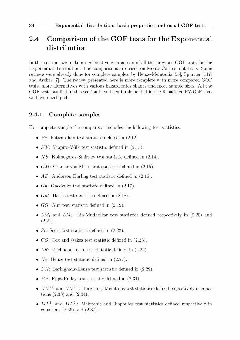
For complete sample the comparison includes the following test statistics:
• Pa: Patwardhan test statistic defined in (2.12).
• SW : Shapiro-Wilk test statistic defined in (2.13).
• KS: Kolmogorov-Smirnov test statistic defined in (2.14).
• CM : Cramer-von-Mises test statistic defined in (2.15).
• AD: Anderson-Darling test statistic defined in (2.16).
• Gn: Gnedenko test statistic defined in (2.17).
• Gn∗: Harris test statistic defined in (2.18).
• GG: Gini test statistic defined in (2.19).
• LM1 and LM2: Lin-Mudholkar test statistics defined respectively in (2.20) and(2.21).
• Sc: Score test statistic defined in (2.22).
• CO: Cox and Oakes test statistic defined in (2.23).
• LR: Likelihood ratio test statistic defined in (2.24).
• He: Henze test statistic defined in (2.27).
• BH: Baringhaus-Henze test statistic defined in (2.29).
• EP : Epps-Pulley test statistic defined in (2.31).
• HM (1) and HM (2): Henze and Meintanis test statistics defined respectively in equa-tions (2.33) and (2.34).
• MI(1) and MI(2): Meintanis and Iliopoulos test statistics defined respectively inequations (2.36) and (2.37).
Exponential distribution: basic properties and usual GOF tests 35
• GW : Grzegorzewski and Wieczorkowski test statistic defined in (2.40).
• BHK and BHC: Baringhaus and Henze test statistics based on the mean residuallife defined in (2.42).
• Kl: Klar test statistic defined in (2.48).
We first simulate iid exponentially distributed samples to verify that the rejection per-centage of the Exponential distribution is close to the theoretical significance level. Then,we simulate samples with the following alternative distributions. For each distribution wegive their pdfs f(x) and hazard rate h(x) when it has an explicit expression:
• The Gamma distribution G(α, λ):
f(x) =λα
Γ(α)exp(−λx)xα−1
• The Lognormal distribution LN (m,σ2):
f(x) =1
xσ√
2πexp
(− 1
2σ2(lnx−m)2
)
• The Uniform distribution U [0, a]:
f(x) =1
a1[0,a](x)
h(x) =1
a− x 1[0,a](x)
• The Inverse-Gamma distribution IG(α, β):
f(x) =βα
Γ(α)x−α−1 exp
(−βx
).
For the sake of simplicity, we adopt the following conventions: scale parameters ofthe Weibull, Gamma and Inverse-Gamma distribution (respectively η, λ and β) are ar-bitrarily set to 1 and the parameter m of the Lognormal distribution is set to 0. Thecorresponding distributions are denoted W(1, β) ≡ W(β), G(α, 1) ≡ G(α), IG(α, 1) ≡IG(α) and LN (0, σ2) ≡ LN (σ2). Parameters of the simulated distributions are selectedto obtain different shapes of the hazard rate:
• IHR: increasing hazard rate
• DHR: decreasing hazard rate
• BT: bathtub-shaped hazard rate
• UBT: upside-down bathtub-shaped hazard rate.
36 Exponential distribution: basic properties and usual GOF tests
For the Exponential case, we use only UBT alternatives. BT alternatives will be also usedfor the Weibull case in the following chapter. Table 2.1 gives the values of the parametersand the notations used for all the simulated distributions:
For a given alternative with fixed parameters and a fixed sample size, we simulate50000 samples of size n ∈ 5, 10, 20, 50.
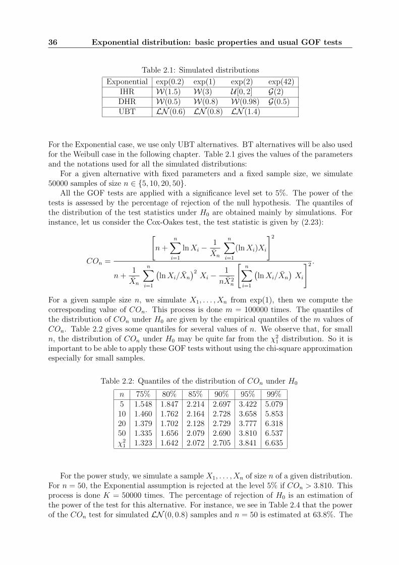
All the GOF tests are applied with a significance level set to 5%. The power of thetests is assessed by the percentage of rejection of the null hypothesis. The quantiles ofthe distribution of the test statistics under H0 are obtained mainly by simulations. Forinstance, let us consider the Cox-Oakes test, the test statistic is given by (2.23):
COn =
[n+
n∑
i=1
lnXi −1
Xn
n∑
i=1
(lnXi)Xi
]2
n+1
Xn
n∑
i=1
(lnXi/Xn
)2Xi −
1
nX2n
[n∑
i=1
(lnXi/Xn
)Xi
]2 .
For a given sample size n, we simulate X1, . . . , Xn from exp(1), then we compute thecorresponding value of COn. This process is done m = 100000 times. The quantiles ofthe distribution of COn under H0 are given by the empirical quantiles of the m values ofCOn. Table 2.2 gives some quantiles for several values of n. We observe that, for smalln, the distribution of COn under H0 may be quite far from the χ2
1 distribution. So it isimportant to be able to apply these GOF tests without using the chi-square approximationespecially for small samples.
Table 2.2: Quantiles of the distribution of COn under H0
For the power study, we simulate a sample X1, . . . , Xn of size n of a given distribution.For n = 50, the Exponential assumption is rejected at the level 5% if COn > 3.810. Thisprocess is done K = 50000 times. The percentage of rejection of H0 is an estimation ofthe power of the test for this alternative. For instance, we see in Table 2.4 that the powerof the COn test for simulated LN (0, 0.8) samples and n = 50 is estimated at 63.8%. The
Exponential distribution: basic properties and usual GOF tests 37
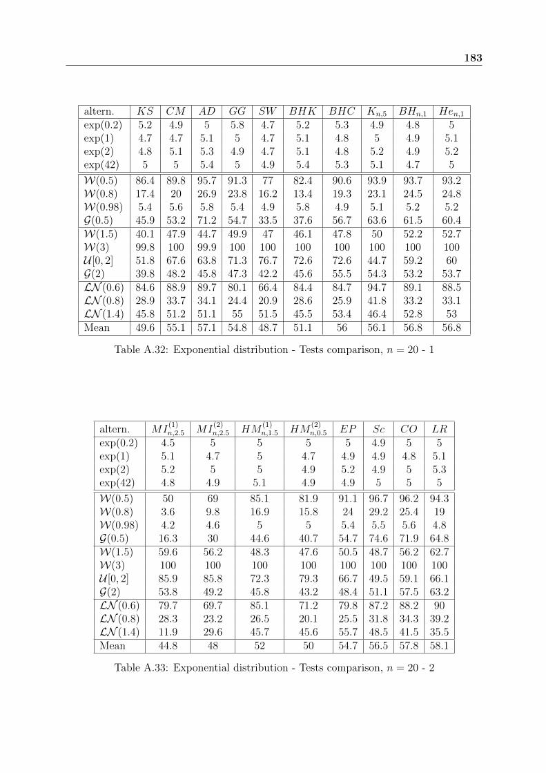
higher the rejection percentage is, the better the test is. We will observe that the resultsare tightly linked to the tested alternatives. In order to evaluate globally the power ofthe tests, we compute for each test the mean value of the rejection percentage for all thealternatives. The power tables of the studied GOF tests are given in Appendix A in orderto avoid a complex and long dissertation in this chapter.
In a first step, the tests are compared inside each family. The choice of parameterssuch as a and m is discussed. In a second step, the best tests of each family are compared.
Tables A.1 and A.2 present the power results for the GOF tests based on the em-pirical distribution function (KS, CM and AD) with and without the application of theK transformation. AD is the best and KS is the worst of the three. The use of the Ktransformation gives better results for some special cases such as the Weibull, LN (1.4)and uniform distributions.
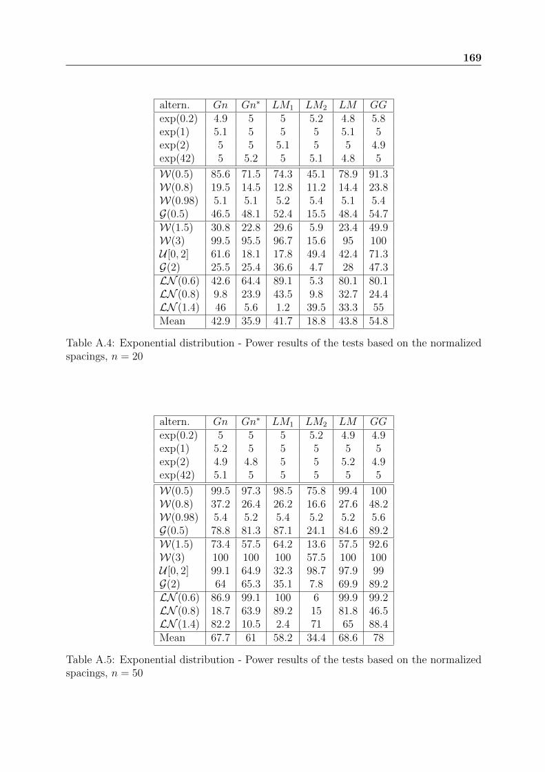
Tables from A.3 to A.5 present the power results of the tests based on the normalizedspacings. GG has the best performance followed by LM .
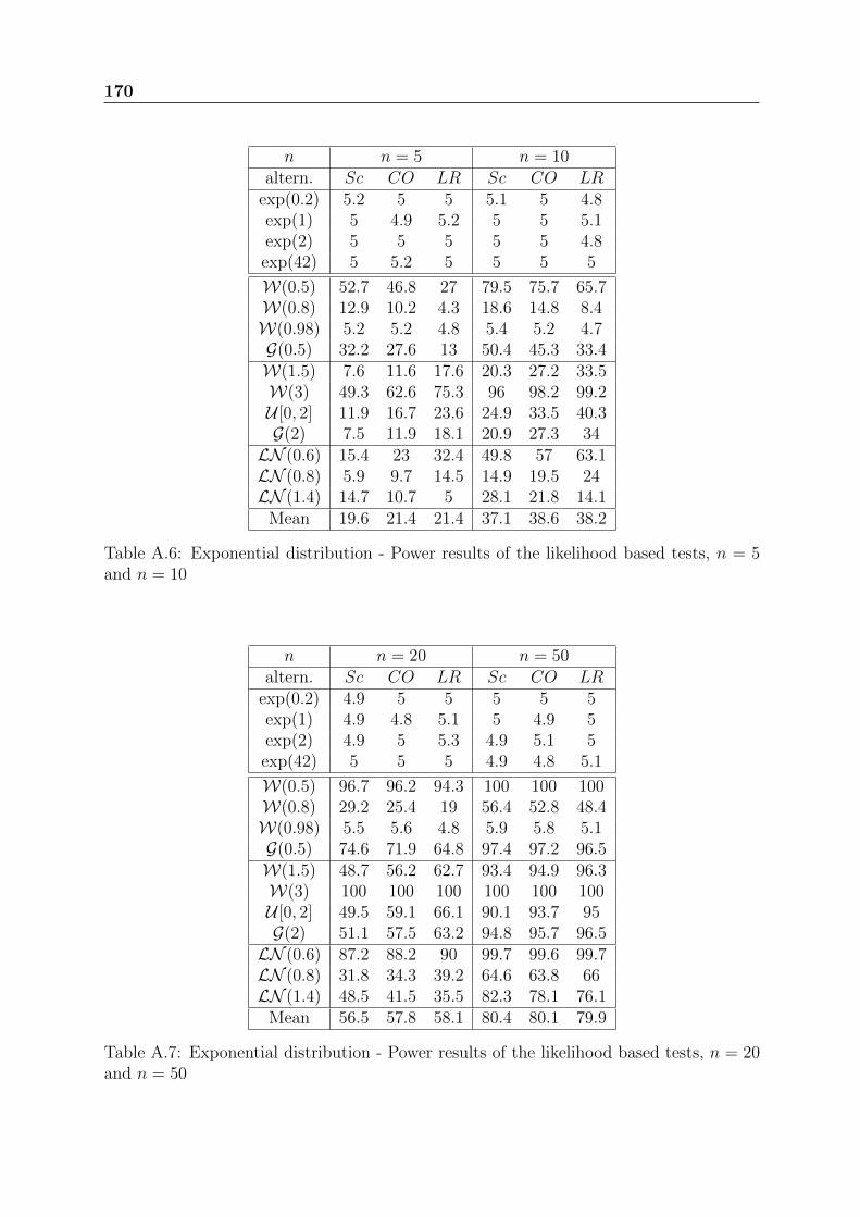
Tables A.6 and A.7 compare the power results for the three likelihood based tests(Sc, CO and LR). It seems clearly that the score test Sc is more appropriate for theDHR alternatives and the test LR based on the likelihood ratio is powerful for the IHRalternatives. The test CO has never been the best one for specific alternatives, but itrepresents an excellent compromise by giving generally good results.
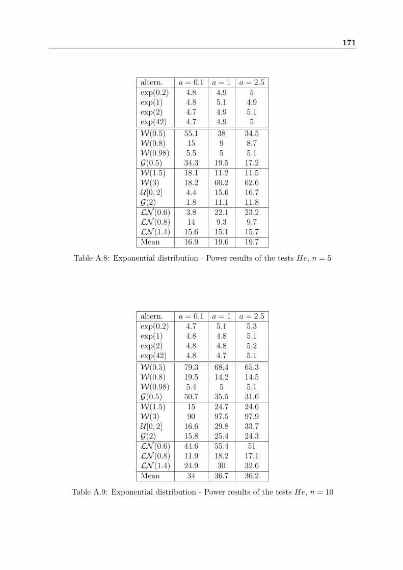
Tables from A.8 to A.11 present the power results of Henze test based on the Laplacetransform. Small values of the parameter a are appropriate for DHR alternatives (W(0.5),W(0.8), G(0.5)), while moderately large values of a, are appropriate to IHR alternatives(W(1.5), W(3), G(2), uniform). The best compromise is made for a = 1.
Tables from A.12 to A.15, present the power results of Baringhaus-Henze test basedon the Laplace transform. The conclusions are similar to those of the previous test. Werecommend also the value a = 1. Baringhaus-Henze test is slightly more powerful thanthe test of Henze.
Tables from A.16 to A.19 present the power results of Henze-Meintanis tests based onthe characteristic function. The power difference between the two tests HM
(1)n,a and HM
(2)n,a
can be very important for some alternatives, for instance: 82.3% and 28.9% for LN (0.8)
distribution with n = 50. Generally, the test HM(1)n,a is more powerful than HM
(2)n,a. But
for DHR alternatives, we recommend the use of HM(2)n,a with large value of the parameter
a. If nothing is known about the tested alternatives, a good compromise is to choose thetest HM
(1)n,a with a = 1.5 for n ≤ 10 and a = 1 for n > 10.
Tables from A.20 to A.22 present the power results of Meintanis-Iliopoulos tests basedon the characteristic function. The fact that the statistics MI
(1)n,a and MI
(2)n,a have more
complex expression than the previous ones, slows down the simulations. These testspresent the characteristic to have extremely weak powers for DHR alternatives and goodones for IHR alternatives. There is no significant difference between MI
(1)n,a and MI
(2)n,a.
We choose a = 2.5, even if the choice of the parameter a has no significant effect on theresults.
Table A.23 presents the power results of Grzegorzewski-Wieczorkowski test based onthe entropy. The choice of the parameter m depends slightly on the tested alternatives.We recommend m = 4 to have the best compromise. This test and Pa test are not verypowerful that is why they will not be presented later in the comparison tables.
Tables A.24 to A.27 present the power results of the test of Klar. For small sizesamples, we should absolutely avoid to choose large values of the parameter a which give
38 Exponential distribution: basic properties and usual GOF tests
null rejection percentages for some alternatives. For n ≥ 20, the best suitable values ofthe parameter a depend on the used alternatives. The best compromise is obtained fora = 5.
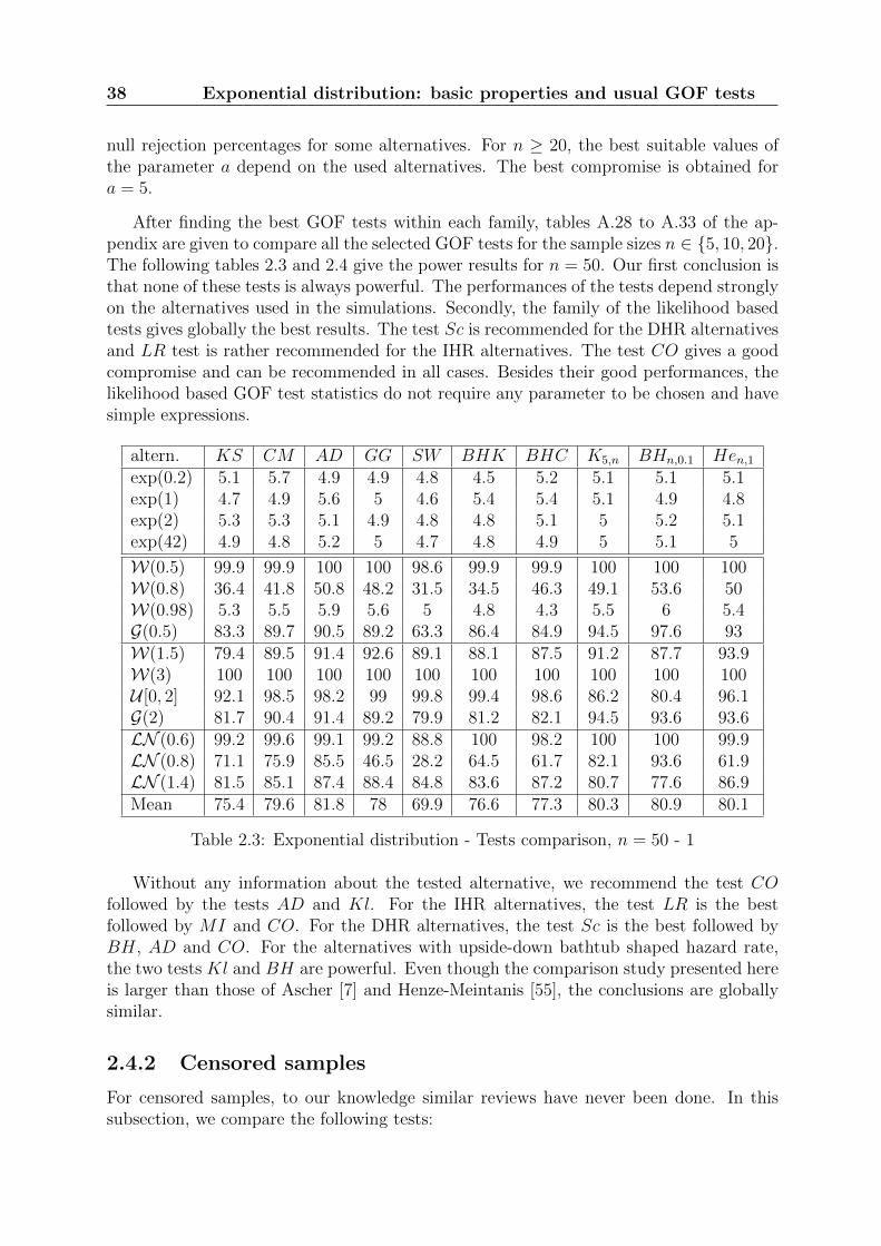
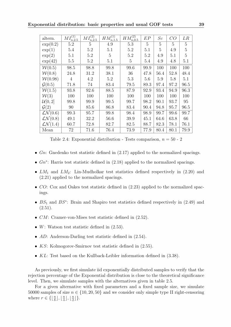
After finding the best GOF tests within each family, tables A.28 to A.33 of the ap-pendix are given to compare all the selected GOF tests for the sample sizes n ∈ 5, 10, 20.The following tables 2.3 and 2.4 give the power results for n = 50. Our first conclusion isthat none of these tests is always powerful. The performances of the tests depend stronglyon the alternatives used in the simulations. Secondly, the family of the likelihood basedtests gives globally the best results. The test Sc is recommended for the DHR alternativesand LR test is rather recommended for the IHR alternatives. The test CO gives a goodcompromise and can be recommended in all cases. Besides their good performances, thelikelihood based GOF test statistics do not require any parameter to be chosen and havesimple expressions.
Table 2.3: Exponential distribution - Tests comparison, n = 50 - 1
Without any information about the tested alternative, we recommend the test COfollowed by the tests AD and Kl. For the IHR alternatives, the test LR is the bestfollowed by MI and CO. For the DHR alternatives, the test Sc is the best followed byBH, AD and CO. For the alternatives with upside-down bathtub shaped hazard rate,the two tests Kl and BH are powerful. Even though the comparison study presented hereis larger than those of Ascher [7] and Henze-Meintanis [55], the conclusions are globallysimilar.
2.4.2 Censored samples
For censored samples, to our knowledge similar reviews have never been done. In thissubsection, we compare the following tests:
Exponential distribution: basic properties and usual GOF tests 39
Table 2.4: Exponential distribution - Tests comparison, n = 50 - 2
• Gn: Gnedenko test statistic defined in (2.17) applied to the normalized spacings.
• Gn∗: Harris test statistic defined in (2.18) applied to the normalized spacings.
• LM1 and LM2: Lin-Mudholkar test statistics defined respectively in (2.20) and(2.21) applied to the normalized spacings.
• CO: Cox and Oakes test statistic defined in (2.23) applied to the normalized spac-ings.
• BS1 and BS∗: Brain and Shapiro test statistics defined respectively in (2.49) and(2.51).
• CM : Cramer-von-Mises test statistic defined in (2.52).
• W : Watson test statistic defined in (2.53).
• AD: Anderson-Darling test statistic defined in (2.54).
• KS: Kolmogorov-Smirnov test statistic defined in (2.55).
• KL: Test based on the Kullback-Leibler information defined in (3.38).
As previously, we first simulate iid exponentially distributed samples to verify that therejection percentage of the Exponential distribution is close to the theoretical significancelevel. Then, we simulate samples with the alternatives given in table 2.5.
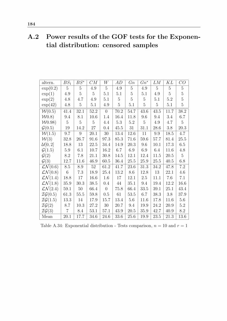
For a given alternative with fixed parameters and a fixed sample size, we simulate50000 samples of size n ∈ 10, 20, 50 and we consider only simple type II right-censoringwhere r ∈ bn
8c, bn
4c, bn
2c.
40 Exponential distribution: basic properties and usual GOF tests
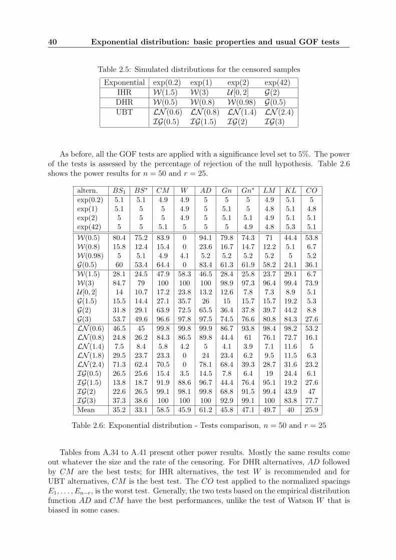
Table 2.5: Simulated distributions for the censored samples
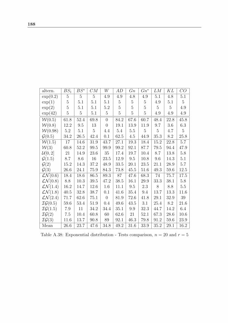
As before, all the GOF tests are applied with a significance level set to 5%. The powerof the tests is assessed by the percentage of rejection of the null hypothesis. Table 2.6shows the power results for n = 50 and r = 25.
Table 2.6: Exponential distribution - Tests comparison, n = 50 and r = 25
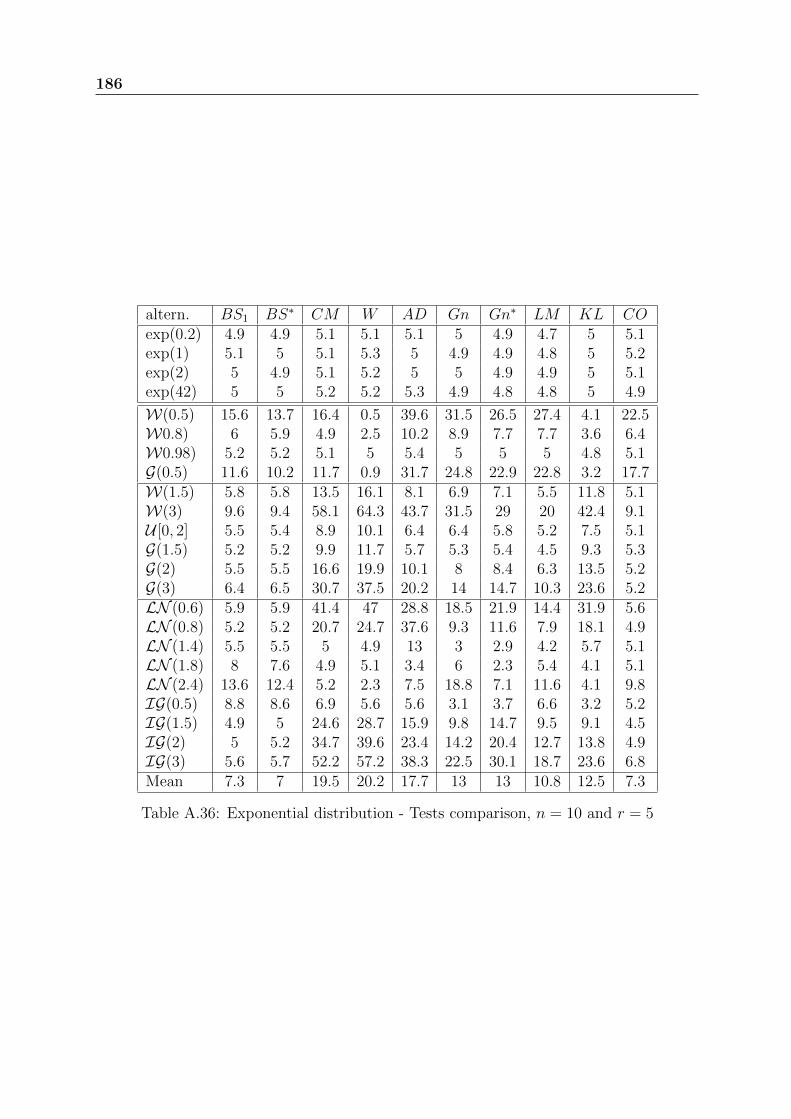
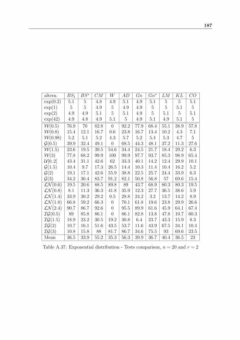
Tables from A.34 to A.41 present other power results. Mostly the same results comeout whatever the size and the rate of the censoring. For DHR alternatives, AD followedby CM are the best tests; for IHR alternatives, the test W is recommended and forUBT alternatives, CM is the best test. The CO test applied to the normalized spacingsE1, . . . , En−r, is the worst test. Generally, the two tests based on the empirical distributionfunction AD and CM have the best performances, unlike the test of Watson W that isbiased in some cases.
Exponential distribution: basic properties and usual GOF tests 41
To sum up, for the censored samples, Anderson-Darling test has the best performancesamong all the studied ones. For the complete samples, the GOF tests of Anderson-DarlingAD, Cox-Oakes CO and the tests based on the empirical characteristic function BH seemto have the best performances. The comparisons were done among 60 GOF tests forcomplete samples and 10 GOF tests for censored samples. All the previous GOF tests forcensored samples are implemented in the R package we have developed EWGoF. A partof this work has been presented in ESREL 2012 conference [70].
The good performance of Cox-Oakes CO test has attracted our attention. That is whywe have developed new GOF tests based on the likelihood for the Weibull distribution(chapter 4).
42 Exponential distribution: basic properties and usual GOF tests
Chapter 3
Weibull distribution: basicproperties and usual GOF tests
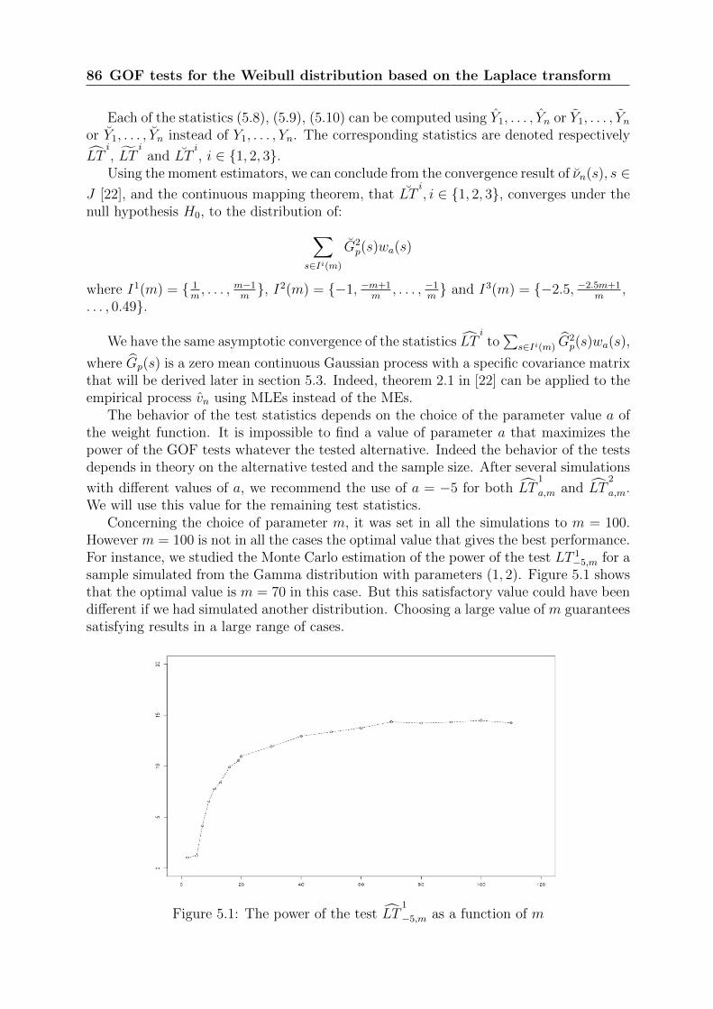
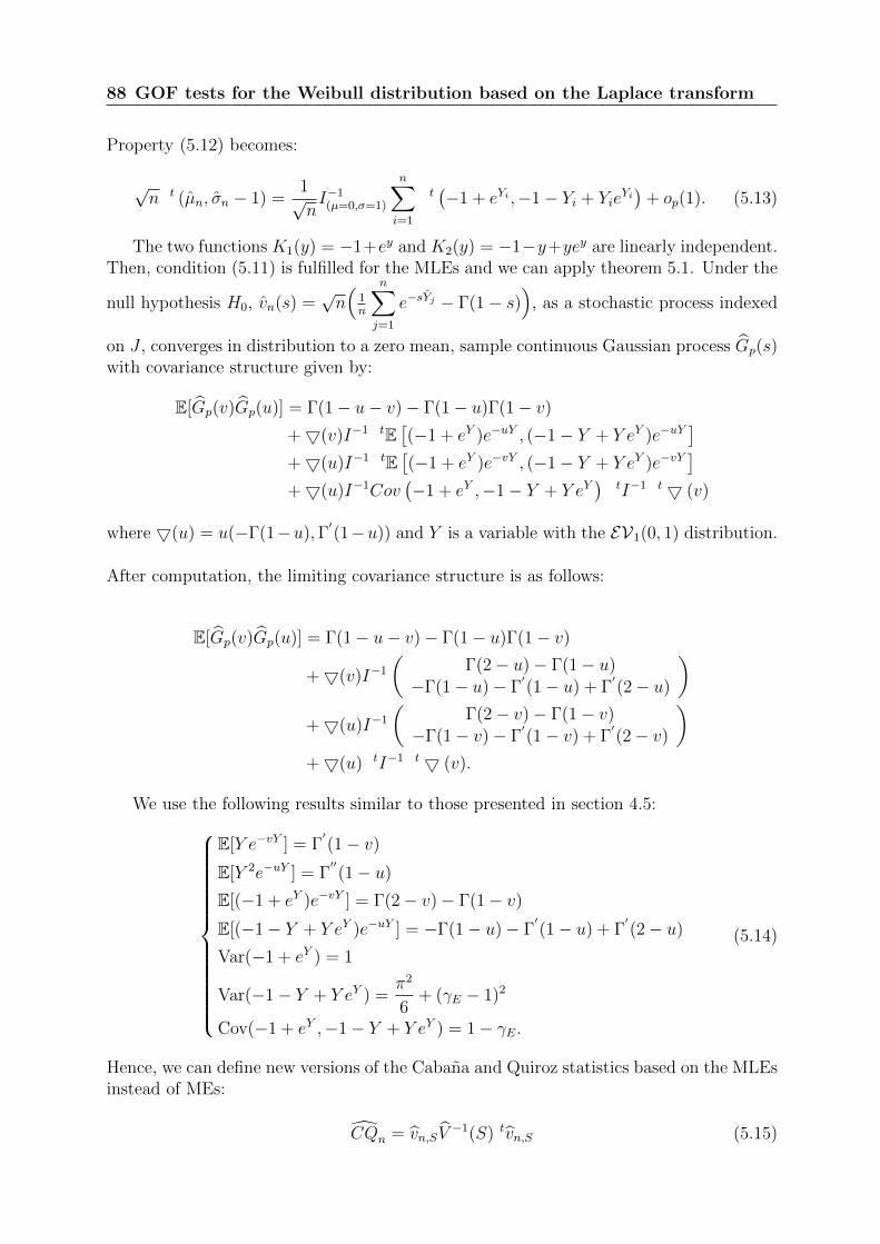
This chapter is dedicated to the two-parameter Weibull distribution. Some definitionsand basic properties of this distribution are given. Then we present a quick review of theusual GOF test for the Weibull distribution. Several GOF tests families are presented suchas tests based on the probability plots, Shapiro-wilk tests, tests based on the empiricaldistribution function, tests based on the normalized spacings, generalized smooth tests,tests based on the Kullback-Leibler information and tests based on the Laplace transform.
3.1 The Weibull distribution: definition and proper-
ties
A random variable X is from the two-parameter Weibull distributionW(η, β), if and onlyif its cdf is:
F (x; η, β) = 1− exp(−(x/η)β), x ≥ 0, η > 0, β > 0. (3.1)
• The pdf of W(η, β) is:
f(x; η, β) =β
η
(x
η
)β−1
exp(−(x/η)β), x ≥ 0, η > 0, β > 0. (3.2)
• The reliability is R(x) = exp(−(xη
)β).
• The expectation is: MTTF = E[X] = ηΓ( 1
β+ 1)
.
• The variance is: V ar(X) = η2Γ( 2
β+ 1)− η2Γ2
( 1
β+ 1)
.
44 Weibull distribution: basic properties and usual GOF tests
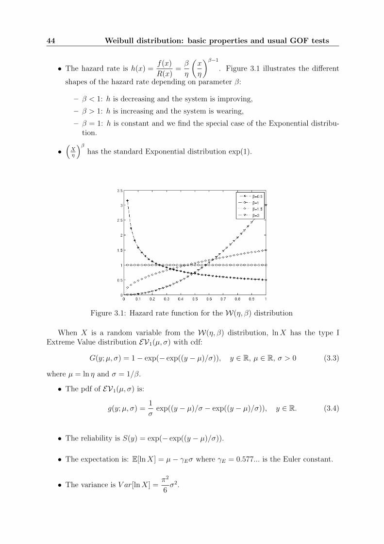
• The hazard rate is h(x) =f(x)
R(x)=β
η
(x
η
)β−1
. Figure 3.1 illustrates the different
shapes of the hazard rate depending on parameter β:
– β < 1: h is decreasing and the system is improving,
– β > 1: h is increasing and the system is wearing,
– β = 1: h is constant and we find the special case of the Exponential distribu-tion.
•(Xη
)βhas the standard Exponential distribution exp(1).
Figure 3.1: Hazard rate function for the W(η, β) distribution
When X is a random variable from the W(η, β) distribution, lnX has the type IExtreme Value distribution EV1(µ, σ) with cdf:
• The reliability is S(y) = exp(− exp((y − µ)/σ)).
• The expectation is: E[lnX] = µ− γEσ where γE = 0.577... is the Euler constant.
• The variance is V ar[lnX] =π2
6σ2.
Weibull distribution: basic properties and usual GOF tests 45
• The hazard rate is h(y) =1
σexp(−(y − µ)/σ).
• The Laplace transform is ψ(t) = E [exp(−t lnX)] = Γ(1− σt
)exp(µt), ∀t > 0.
• Y = β ln(X/η) = (lnX − µ)/σ follows EV1(0, 1).
Let X1, . . . , Xn be n (iid) random variables from theW(η, β) distribution. We considerthree methods for estimating the parameters η and β: the maximum likelihood, leastsquares and moment methods.
• The maximum likelihood estimators (MLEs) of η and β, ηn and βn, are solutions ofthe following equations:
ηn =
(1
n
n∑
i=1
X βni
)1/βn
n
βn+
n∑
i=1
lnXi −n
n∑
i=1
X βni
n∑
i=1
X βni lnXi = 0.
(3.5)
• The Weibull probability plot (WPP) [92] is the plot of points:
(lnX∗i , ci) , i ∈ 1, . . . , n (3.6)
where ci = ln [− ln (1− pi)] and pi, i ∈ 1, . . . , n, are approximations of the orderstatistics of a uniform sample. Usual choices are symmetrical ranks pi = (i− 0.5)/nand mean ranks pi = i/(n+ 1). Under the Weibull assumption, these points shouldbe approximately on a straight line [31].
The least squares estimators (LSEs) based on the WPP, ηn and βn, are defined asfollows [76]:
βn =
n∑
i=1
(ci − c)2
n∑
i=1
(lnXi − lnX)(ci − c)
ln ηn = lnX − c
βn
(3.7)
where lnX =1
n
n∑
i=1
lnXi and c =1
n
n∑
i=1
ci.
46 Weibull distribution: basic properties and usual GOF tests
• The moment estimators (MEs), ηn and βn, are defined as follows [111]:
βn =π√6
[1
n− 1
n∑
i=1
(lnXi − lnX)2
]−1/2
ln ηn = lnX +γE
βn
(3.8)
For all i ∈ 1, . . . , n, Yi = β ln(Xi/η) has the EV1(0, 1) distribution. The orderstatistics of this sample are denoted Y ∗1 ≤ . . . ≤ Y ∗n .
Since η and β are unknown, it will be useful in the following to replace them bythe above estimators. For all i, let Yi = βn ln(Xi/ηn), Yi = βn ln(Xi/ηn) and Yi =
βn ln(Xi/ηn). It is expected that the distributions of Yi, Yi and Yi will not be far fromthe EV1(0, 1) distribution.
From [6], the distribution of (Y1, . . . , Yn) does not depend on η and β. From [76], it is
also the case of the distribution of (Y1, . . . , Yn). The following property proves the sameresult for (Y1, . . . , Yn).
Property 3.1 The distribution of (Y1, . . . , Yn) does not depend on η and β.
Proof: We know that ∀i ∈ 1, . . . , n, lnXi =Yiβ
+ ln η. So:
Yi = βn(lnXi − ln ηn) = βn
(Yiβ− Y
β− γE
βn
)(3.9)
where Y =1
n
n∑
i=1
Yi = β(lnX − ln η).
Moreover, S2 =S2Y
β2, so βn = β
π√6SY
, where SY =
[1
n− 1
n∑
i=1
(Yi − Y )2
]1/2
. Hence:
Yi =π√6SY
(Yi − Y )− γE. (3.10)
Since the distribution of (Y1, . . . , Yn) does not depend on η and β, it is also the case forthe distribution of (Y1, . . . , Yn) and the property is proved.
The fact that the distributions of the samples Yi, Yi and Yi are independent of theparameters of the underlying Weibull distribution is a very fundamental property sinceit allows to build GOF test statistics as functions of these samples. If a statistic S is afunction of the Yi, we will denote S, S and S the same statistic as a function of respectivelythe Yi, Yi and Yi.The normalized spacings of the Extreme Value distribution Ei are:
∀i ∈ 1, . . . , n, Ei =lnX∗i − lnX∗i−1
E[
lnX∗i − µσ
]− E
[lnX∗i−1 − µ
σ
] = σY ∗i − Y ∗i−1
E[Y ∗i − Y ∗i−1
] . (3.11)
Weibull distribution: basic properties and usual GOF tests 47
Pyke [104] proved that for any distribution verifying given conditions, an appropriatesubset of the normalized spacings Ei constitutes a vector whose components are asymp-totically independent and exponentially distributed. These results are exact in the caseof the Exponential distribution and asymptotic for the Extreme Value distribution. Thevalues of the expectations E [Y ∗i ] are known and have explicit expressions given in [121].
3.2 Usual GOF tests for the Weibull distribution
In this section, we present families of GOF tests for the Weibull distribution. There existseveral families such as tests based on the Weibull probability plot, tests based on theempirical distribution function, tests based on the normalized spacings, tests based onthe Laplace transform, ... Thanks to a logarithmic transformation, these GOF tests canalso be used as GOF tests for the Extreme Value distribution.
3.2.1 Tests based on probability plots
We remind that the Weibull probability plot is the plot of points:
(lnX∗i , ci) , i ∈ 1, . . . , n
where ci = ln [− ln (1− pi)] and pi, i ∈ 1, . . . , n, are approximations of the order statis-tics of a uniform sample. Under the Weibull assumption, these points should be approx-imately on a straight line.
Smith and Bain [115] used the determination coefficient R2SB of the ordinary least
squares to build a GOF test. The test is based on the statistic Z2 = n(1−R2SB), where
R2SB =
[n∑
i=1
(lnX∗i − lnX) (ci − cn)
]2
n∑
i=1
(lnX∗i − lnX)2
n∑
i=1
(ci − cn)2
(3.12)
with ci = ln [− ln (1− pi)] , i = 1, ..., n, cn = 1n
n∑
i=1
ci and pi = in+1
(mean ranks).
The test rejects the null hypothesis when Z2 is too close to 1. Evans, Johnson and Green
[42] proposed a GOF test based on a statistic similar to R2SB:
R2EJG =
[n∑
i=1
(lnX∗i − lnX)Mi
]2
n∑
i=1
(lnX∗i − lnX)2
n∑
i=1
(Mi −Mn)2
(3.13)
where Mi =1
βnln
[− ln
(1− i− 0.3175
n+ 0.365
)].
48 Weibull distribution: basic properties and usual GOF tests
The stabilized probability plot [87] is an alternative to the probability plot, which aimsto stabilize the variance of the plotted points. It is defined as the sets of points (ri, si),i ∈ 1, . . . , n, where:
ri =2
πarcsin
√i− 0.5
nand si =
2
πarcsin
√
1− exp
(−(X∗iηn
)βn ). (3.14)
Under the Weibull assumption, these points should be approximately on the line y = x.Coles [28] proposed to measure the departure from this line by the statistic:
SPPn = max1≤i≤n
|ri − si|. (3.15)
He used Blom estimators [17] instead of MLEs. Kimber [64] gave the quantiles tablesof the statistic SPPn using an approximation of the best unbiased linear estimators.
3.2.2 Shapiro-Wilk type tests
Shapiro and Brain [115] and Ozturk and Korukoglu [97] adapted the idea of Shapiro-WilkGOF test of exponentiality. The idea of the test is to compute the ratio of two estimatorsof 1
β. The first estimator is a linear combination of the lnX∗i , suggested by d’Agostino
[30]:
1
n
n∑
i=1
[0.6079wn+i − 0.257wi] lnX∗i (3.16)
where the wi are defined as follows:
wi = lnn+ 1
n− i+ 1∀i ∈ 1, . . . , n− 1
wn = n−n−1∑
i=1
wi
wn+i = wi(1 + lnwi)− 1 ∀i ∈ 1, . . . , n− 1
w2n = 0.4228n−n−1∑
i=1
wn+i.
The second estimator proposed by Shapiro and Brain [112] is the empirical standarddeviation of the lnX∗i . The corresponding statistic has the following expression:
SBn =
(1
n
n∑
i=1
[0.6079wn+i − 0.257wi] lnX∗i
)2
1
n
n∑
i=1
(lnX∗i − lnX)2
. (3.17)
The second estimator used by Ozturk and Korukoglu [97] is another linear combinationof the lnX∗i :
n∑
i=1
(2i− n− 1) lnX∗i
ln 2n(n− 1). (3.18)
Weibull distribution: basic properties and usual GOF tests 49
The corresponding statistic is:
OKn =
ln 2 (n− 1)n∑
i=1
[0.6079wn+i − 0.257wi] lnX∗i
n∑
i=1
(2i− n− 1) lnX∗i
. (3.19)
Ozturk and Korukoglu recommended using the following standardized statistic thatimproves the performance of the test:
OK∗n =OKn − 1− 0.13/
√n+ 1.18/n
0.49/√n− 0.36/n
. (3.20)
For the two GOF tests SBn and OK∗n, the null hypothesis H0 is rejected when the valueof the statistic (the ratio of two estimators of 1
β) is too far from 1. Thus the rejection is
pronounced for too small or too large values of the statistic.
3.2.3 Tests based on the empirical distribution function
These tests are based on a measure of the departure between the empirical cdf of the
lnXi: Gn(x) =1
n
n∑
i=1
1lnXi≤x and the estimated theoretical cdf using the MLEs G0(y) =
G(y; ln ηn, 1/βn). The null hypothesis is rejected when this difference is too large. Theusual tests based on the empirical cdf can be used only when the tested distribution haslocation-scale parameters. It is the case of the Extreme Value distribution that is why weuse the empirical cdf of lnXi instead of the one of Xi. The best known statistics [25, 31]as those for the Exponential distribution previously defined in subsection 2.2.4 are:
• Kolmogorov-Smirnov statistic (KS):
KSn =√n supy∈IR
∣∣∣Gn(y)− G0(y)∣∣∣ (3.21)
=√nmax
[max
( in− U∗i , i = 1 : n
),max
(U∗i −
i− 1
n, i = 1 : n
)](3.22)
• Cramer-von Mises statistic (CM):
CMn = n
∫ +∞
−∞
[Gn(y)− G0(y)
]2
dG0(y) =n∑
i=1
(U∗i −
2i− 1
2n
)2
+1
12n(3.23)
• Anderson-Darling statistic (AD):
ADn = n
∫ +∞
−∞
[Gn(y)− G0(y)
]2
G0(y)(1− G0(y))dG0(y) (3.24)
= −n+1
n
n∑
i=1
[(2i− 1− 2n) ln(1− U∗i ))− (2i− 1) ln(U∗i )
](3.25)
50 Weibull distribution: basic properties and usual GOF tests
Liao and Shimokawa [76] have proposed to replace the MLEs by the LSEs in (3.22),
(3.23) and (3.25). For instance, the ADn statistic will be denoted ADn when used with
the MLEs and ADn when used with the LSEs. Liao and Shimokawa [76] also combinedthe ideas of Kolmogorov-Smirnov and Anderson-Darling statistics with the LSEs insteadof the MLEs. They proposed the statistic:
LSn =1√n
n∑
i=1
max∣∣∣Gn(lnXi)− G0(lnXi)
∣∣∣√G0(lnXi)(1− G0(lnXi))
=1√n
n∑
i=1
max[in− U∗i , U∗i − i−1
n
]
√U∗i (1− U∗i )
(3.26)
where G0(y) = G(y; ln ηn, 1/βn) = 1− exp(− exp(βn(y − ln ηn))) and Ui = G0(lnXi).
They recommended the use of LSn or ADn.
3.2.4 Tests based on the normalized spacings
The normalized spacings are defined as:
∀i ∈ 1, . . . , n, Ei =lnX∗i − lnX∗i−1
E[
lnX∗i − µσ
]− E
[lnX∗i−1 − µ
σ
] = σY ∗i − Y ∗i−1
E[Y ∗i − Y ∗i−1
] . (3.27)
Every statistic of the form
∑
i
aiEi
∑
j
bjEjcan be used as a test statistic because it has a
distribution that is independent of the two parameters η and β.
Mann, Scheuer and Fertig [82] used the fact that for i ∈ 1, . . . , n, the Ei/σ areasymptotically independent and distributed according to a standard Exponential distri-bution [104]. The authors proposed the statistic:
MSFn =
n∑
j=bn2 c+2
Ej
n∑
j=2
Ej
(3.28)
where bxc is the floor of x. Under H0, MSFn is asymptotically distributed accordingto the beta distribution β
(⌊n−1
2
⌋,⌊n2
⌋). The Weibull assumption is rejected for both
large and small values of the statistic. For usual alternatives, Mann, Sheuer and Fertig
Weibull distribution: basic properties and usual GOF tests 51
recommended rejecting the null hypothesis only for large values of the statistic. Thiswrong use of the test improves its power in some cases, but leads to a biased test.
Tiku and Singh [121] suggested to reject the Weibull hypothesis for both large andsmall values of the statistic:
TSn =
2n−1∑
i=2
(n− i)Ei
(n− 2)n∑
i=2
Ei
. (3.29)
Under H0,√
3(n− 2) (TSn − 1) has asymptotically the normal distribution N(0, 1).
Lockhart, O’Reilly and Stephens [81] used the random variables:
Zj =
j∑
i=2
Ei/
n∑
i=2
Ei, j = 2, . . . , n− 1. (3.30)
Under H0, the Zj are approximately distributed as the order statistics of the uniformdistribution U [0, 1]. Then, Lockhart et al proposed a GOF test based on the Anderson-Darling statistic computed for the Zj:
LOSn = 2− n− 1
n− 2
n−1∑
i=2
[(2(i− n) + 1) ln(1− Zi)− (2i− 3) lnZi]. (3.31)
The previous statistics MSFn and TSn are based respectively on the median and themean value of the sample Zi as it was discussed in [81]. Other test statistics can beapplied to test the uniformity of the sample Zi such as the Cramer-Von-Mises statistic.
These tests require the computation of the expectations of the order statistics of thestandard Extreme Value distributions (E[Y ∗i ]) which makes the use of these statistics notstraightforward.
3.2.5 Generalized smooth tests
The principle of these tests consists in nesting the tested pdf g of the sample lnX1, . . . , lnXn
within an order k alternative [107]:
gk(y; θ, µ, σ) = C(θ, µ, σ) exp
(k∑
i=1
θihi(y;µ, σ)
)g(y;µ, σ) (3.32)
where θT = (θ1, . . . , θk) and hi(y, µ, σ), i ∈ 1, . . . , k, are orthonormal functions ong(y;µ, σ) and C(θ, µ, σ) is a normalizing constant. Testing the Weibull assumption is
equivalent to test H0: “θ = 0” vs H1: “θ 6= 0”. Generalized score test statistic of orderk can be used to test the null hypothesis H0. The test statistic is a quadratic form ofthe vector (ST1, . . . , STk) where STi = 1√
nhi(Yi). Each single component STi of the test
52 Weibull distribution: basic properties and usual GOF tests
statistic can be used as a test statistic.The orthonormal polynomial functions used in the case of the Extreme Value distributionare given in Appendix C of [107]. Using the moment estimators of the parameters given inequation (3.8), the test statistics have simpler expressions and can be easily interpreted. Ithas been shown in [16] that the two first non-zero components are related to the skewnessand the kurtosis coefficients of the sample Yi. They have the following expressions:
ST 3 = −√
b1 + 1.139547/√
20/n (3.33)
ST 4 =b2 + 7.55
√b1 + 3.21
/√
219.72/n (3.34)
where√b1 and b2 are, respectively, the sample skewness and kurtosis defined by:
√b1 =
1
n
n∑
j=1
(lnXi − lnX)3/[ 1
n
n∑
j=1
(lnXi − lnX)2]3/2
(3.35)
b2 =1
n
n∑
j=1
(lnXj − lnX)4/[ 1
n
n∑
j=1
(lnXi − lnX)2]2
. (3.36)
The rejection of H0 is done for large values of the statistics.
3.2.6 Tests based on the Kullback-Leibler information
The following GOF test for the Extreme Value distribution is based on the Kullback-Leibler information [123]. The test can be applied to the sample lnX1, . . . , lnXn with thepdf g. The Kullback-Leibler discrimination information between g and g is:
KL(g, g) =
∫ +∞
−∞g(y) ln
g(y)
g(y; µn, σn)dy =
∫ +∞
−∞g(y) ln(g(y)) dy −
∫ +∞
−∞g(y) ln(g(y)) dy.
(3.37)To evaluate KL(g, g), the first term of (3.37) is estimated by the Vasicek estimator
Hm,n = 1n
n∑
i=1
ln[ n
2m(lnX∗i+m − lnX∗i−m)
]where m < bn/2c, X∗j = X∗1 if j < 1, X∗j =
X∗n if j > n. Note that this estimation is computed for the lnXi while the simi-lar one in equation (2.38) was computed for the Yi. The second term is estimated by
1n
n∑
i=1
ln g(lnXi; µn, σn). Thus KL can be estimated by:
KLm,n = − 1
n
n∑
i=1
ln[ n
2m(Y ∗i+m − Y ∗i−m)
]− 1
n
n∑
i=1
Yi +1
n
n∑
i=1
eYi . (3.38)
The null hypothesis H0 is rejected for large values of the statistic KLm,n. The values of
the parameter m are given in [38]. This test can have two additional versions KL andKL using respectively the least squares and the moment estimators.
Weibull distribution: basic properties and usual GOF tests 53
3.2.7 Tests based on the Laplace transform
Cabana and Quiroz [22] used the Laplace transform to build GOF tests for the Weibulland type I Extreme Value distributions.
We remind that the Laplace transform of a sample Y1, ..., Yn from the EV1(0, 1) dis-tribution is:
ψ(t) = E[e−tY
]= Γ(1− t), ∀t < 1. (3.39)
Cabana and Quiroz proposed to estimate ψ(t) by the empirical Laplace transform
ψn(t) = 1n
∑nj=1 e
−tYj using the moment estimators.Their statistic is based on the closeness between the empirical and theoretical Laplace
transform which is measured by the empirical moment generating process:
vn(s) =√n( 1
n
n∑
j=1
e−Yjs − Γ(1− s)). (3.40)
They proved the convergence, under H0, of vn(s), s ∈ J , to a Gaussian process Gp(s),for some interval J . They recommended to choose J ⊆ [−2.5, 0.49] and suggested twotest statistics based on vn. The first one has the following quadratic form:
CQn = vn,SV−1(S) tvn,S (3.41)
where vn,S = (vn(s1), . . . , vn(sk)), S = s1, . . . , sk ⊂ J and V (S) is the limiting covari-
ance matrix of vn,S given in equation (2.7) in [22]. The statistic CQn has a limiting χ2
distribution with k degrees of freedom under the null hypothesis H0. The second teststatistic is similar to the test of Henze: it is based on a weighted L2 norm. The onlydifference being the choice of the weight function that is different from the one used byHenze:
Sn =
∫
J
v2n(s)/V (s) ds (3.42)
where V is the limiting variance of vn. The asymptotic distribution of the test statistic Snconverges to the distribution of
∫JG2p(s)/V (s) ds. The rejection of the Weibull assumption
is done for large values of the statistics.
In this chapter we presented a complete review of existing GOF tests for the Weibulldistribution. All the previous GOF tests will be compared later in chapter 6 with the newdeveloped GOF tests presented in chapters 4 and 5. All these GOF tests are implementedin our R package EWGoF.
54 Weibull distribution: basic properties and usual GOF tests
Chapter 4
Simplified likelihood based GOFtests for the Weibull distribution
The aim of this chapter is to present new likelihood based GOF tests for the Weibulldistribution. These tests consist in nesting the Weibull distribution in three-parametergeneralized Weibull families [92, 101] and testing the value of the third parameter by usingthe Wald, score and likelihood ratio procedures. We simplify the usual likelihood basedtests by getting rid of the nuisance parameters, using the three estimation methods pre-sented previously in chapter 3: maximum likelihood, least squares and moment methods.The proposed tests are exact.
The Weibull distribution is embedded in generalized Weibull distributions, which havebeen proposed in order to take into account bathtub-shaped or upside-down bathtubshaped hazard rates. A comprehensive comparison study is presented. Theoretical asymp-totic results are derived when the Weibull distribution is nested in the generalized Gammadistribution.
4.1 Generalized Weibull distributions GWMany generalizations of the Weibull distribution have been proposed in order to take intoaccount more general shapes of the hazard rate such as bathtub-shaped or upside-downbathtub-shaped [92, 101], until very recently [96, 114, 4]. Most of them have three pa-rameters θ = (θ, η, β)
′, and, for a value θ0 of θ, they reduce to the two-parameter Weibull
distribution. These distributions will be called here generalized Weibull distributions andwill be denoted GW(θ, η, β). Then, GW(θ0, η, β) =W(η, β).
For a given data set, it is interesting to determine if the simple Weibull distribution isan adapted model or if a more sophisticated model is needed. Then, within a particularGW(θ, η, β) model, it is worthwhile to build a statistical test of H0: “θ = θ0” vs H1:“θ 6= θ0”. Such a test can be considered as a GOF test for the Weibull distribution,because H0 corresponds to the assumption that the distribution of the data is Weibull,even if H1 is a more constrained hypothesis than the initial alternative. This approachis similar to that of the Cox-Oakes test defined in equation (2.23), which is a GOF test
56 Simplified likelihood based GOF tests for the Weibull distribution
of exponentiality based on the inclusion of the Exponential distribution in the Weibullfamily. We showed in chapter 2 that this test is one of the most powerful GOF tests forthe Exponential distribution. That is why we use the same approach to build new GOFtests for the Weibull distribution.
Table 4.1 presents the generalized Weibull distributions used in this work, mainlyselected from [92]. All these distributions are defined on R+, as the standard Weibull, soin the table, x ≥ 0. For each distribution, the table gives its name, its cdf FX , the valueθ0 of parameter θ for which the distribution is Weibull, and describes the possible shapesof the hazard rate.
For instance, Figures 4.1 and 4.2 present the 4 types of shape of the hazard rate ofrespectively the Exponentiated Weibull and the Generalized Gamma distributions [88,118].
For the Generalized Weibull distribution introduced in [89], we consider only the caseof unbounded lifetimes, corresponding to λ > 0. In this case, the distribution is linkedto the Burr type XII distribution [21], so we will call it the Burr Generalized Weibulldistribution.
For the Additive Weibull distribution, we consider the special case with three param-eters instead of four, which happens to be also the B distribution [15].
*
0 10 20 30 40 50 60 70 80 90 100
0
0.01
0.02
0.03
0.04
0.05
0.06
0.07
0.08
0.09
0.1
EW(0.1, 100, 5)
EW(4, 12, 0.6)
EW(0.5, 100, 0.5)
EW(4, 85, 4)
Figure 4.1: Shapes of the hazard rate for the Exponentiated Weibull distribution
Simplified likelihood based GOF tests for the Weibull distribution 57
BGW(λ, η, β) [89] λ, η, β > 0 DHR if β < 1UBT if β > 1
Marshall-Olkin FX(x;α, η, β) = 1− αe−(x/η)β
1−(1−α)e−(x/η)βWeibull if α = 1
Extended Weibull α, η, β > 0 IHR if α ≥ 1 and β ≥ 1MO(α, η, β) [83] DHR if α ≤ 1 and β ≤ 1
other shapes
Modified Weibull FX(x; ρ, η, β) = 1− e−(xη
)βeρxWeibull if ρ→ 0
MW(ρ, η, β) [72] ρ, η, β > 0 IHR if β > 1BT if 0 < β < 1
Power Generalized Weibull FX(x; ν, η, β) = 1− e1−(1+(x/η)β)1ν
Weibull if ν = 1PGW(ν, η, β) [94] ν, η, β > 0 IHR if β > 1 and β > ν
DHR if 0 < β < 1 and β ≤ νBT if 0 < ν < β < 1UBT if ν > β > 1
58 Simplified likelihood based GOF tests for the Weibull distribution
Figure 4.2: Shapes of the hazard rate for the Generalized Gamma distribution
4.2 Likelihood based goodness-of-fit tests
Let us assume that X1, ..., Xn are from a generalized Weibull distribution GW(θ), withpdf f(x;θ), where θ = (θ, η, β)
′. When θ = θ0, the Xi have the W(η, β) distribution.
So we want to test the null hypothesis H0: “θ = θ0” vs H1: “θ 6= θ0”, where (η, β) is anuisance parameter.
The tests studied are the Wald, score and likelihood ratio tests, which are based onthe asymptotic properties of the maximum likelihood estimators. The likelihood functionfor θ is:
L(θ) =n∏
i=1
f(xi;θ). (4.1)
Let θn = (θn, ηn, βn)′
be the MLE of θ, value at which L(θ) is maximized. The scorevector is U(θ) = ∇ lnL(θ).
The Fisher matrix is the covariance matrix of the score. Since it is often difficult tocompute, it is more convenient to use the observed Fisher information matrix I(θ). Sinceθ is partitioned in θ and (η, β), we partition U(θ) and I(θ) in the same way, so that thescore and observed information matrix can be written:
U(θ) =
(U1(θ)U2(θ)
)and I(θ) =
(I11(θ) I12(θ)I21(θ) I22(θ)
). (4.2)
The inverse of I(θ) is denoted:
I(θ)−1 =
(I11(θ) I12(θ)I21(θ) I22(θ)
).
Simplified likelihood based GOF tests for the Weibull distribution 59
For a given value θ0 of θ, let (ηn(θ0), βn(θ0)) denotes the profile MLE of (η, β),obtained by maximizing the profile likelihood L(θ0, η, β) with respect to (η, β). Letθn = (θ0, ηn(θ0), βn(θ0)).
The Wald, score and likelihood ratio statistics are respectively [74]:
W =(θn − θ0)2
I11(θn), (4.3)
Sc = U1(θn)2I11(θn), (4.4)
LR = −2 lnL(θn)
L(θn). (4.5)
Under the null hypothesis H0, these statistics converge to the χ21 distribution when n
tends to infinity [74]. The (asymptotic) tests consist in rejecting the Weibull assumptionH0 at the significance level α, if the statistics are greater than the quantile of order (1−α)of the χ2
1 distribution.This approach has been used by Mudholkar-Srivastava [88], Mudholkar et al [89],
Bousquet et al [15] and Caroni [23], who nested the Weibull distribution in respectively theexponentiated Weibull [88], Burr generalized Weibull [89], a particular additive Weibull[15] and the Marshall-Olkin extended Weibull [83] distributions. In these papers, the aimof the tests is to confirm that the considered generalized distribution is needed instead ofthe basic Weibull. In each case, the asymptotic tests are used, with the χ2
1 distribution.But this can lead to significant errors for small samples. For instance, Caroni showedthat the chi-square approximation for the distribution of the score statistics is still notsatisfactory for n = 200. Moreover, a simulation study showed that the distributionsunder H0 of the Wald, score and likelihood ratio statistics may depend on η and β in thecase of small samples. Finally, the computation of θn and θn may be difficult for somegeneralized Weibull distributions.
Since we want to use this kind of tests for small samples and for a large spectrum ofgeneralized Weibull distributions, we propose another approach. The first idea is to movefrom the Weibull to the extreme value distribution with the logarithmic transformation.Let us recall that the Yi = β ln(Xi/η) are a sample of the EV1(0, 1) distribution. The nicefact is that this distribution has no unknown parameter. Using the idea of likelihood basedtests, the EV1(0, 1) distribution can be included in a larger family with only one parameterθ. We can call these families generalized extreme value distributions and denote themGEV(θ). It is possible to derive likelihood based tests of H0: “θ = θ0” vs H1: “θ 6= θ0”in these families. This situation is simpler than the previous one because there are nonuisance parameters.
In fact, these tests can not be used directly since η and β are unknown, so the Yi arenot observed. Given that the Yi, can be approximated by the Yi, Yi and Yi, previouslydefined in section 3.1, our proposal is to test that the Xi come from a Weibull distributionby testing that the Yi, Yi or Yi come from the EV1(0, 1) distribution using the Wald, scoreor likelihood ratio tests.
Now we have to choose a particular GEV(θ) family. Since only parameter θ is con-cerned, we can use the link between Weibull and extreme value distributions when η =
60 Simplified likelihood based GOF tests for the Weibull distribution
β = 1. So we will define a GEV(θ) distribution as the distribution of lnX, when X has aGW(θ, 1, 1) distribution.
This approach is summarized in the following steps:
1. Choose a generalized Weibull family GW(θ, η, β). Let FX(x; θ, η, β) be its cdf andfX(x; θ, η, β) be its pdf.
2. Compute the pdf of Y = lnX when η = β = 1:
fY (y; θ) = eyfX(ey; θ, 1, 1).
3. Compute the likelihood L(θ) =n∏i=1
fY (yi; θ) and the MLE of θ, θn. The computation
of θn is of course much easier than that of θn in the first approach.
4. Compute the score and observed information:
U(θ) =∂ lnL(θ)
∂θ, (4.6)
I(θ) = −∂2 lnL(θ)
∂θ2. (4.7)
Note that the score and information are here unidimensional, so their computationis much easier than in the first approach (4.2).
5. The likelihood based statistics are:
W = I(θ0)(θn − θ0)2, (4.8)
Sc =U2(θ0)
I(θ0), (4.9)
LR = −2 lnL(θ0)
L(θn). (4.10)
The expressions of these statistics are much simpler than that of the correspondingstatistics in the first approach. The fact that Sc does not depend on θn is generallyvery convenient, but sometimes, this leads to undefined statistics. Then, it will beuseful to use Slutsky’s theorem and define W and Sc as:
W = I(θn)(θn − θ0)2, (4.11)
Sc =U2(θ0)
I(θn). (4.12)
6. In the expressions of θn, W , Sc and LR, replace Yi by Yi. If T denotes a particularGW model chosen, the corresponding statistics are denoted Tw, Ts and Tl.
Do the same thing with Yi and Yi and derive Tw, Ts, Tl, Tw, Ts and Tl.
Simplified likelihood based GOF tests for the Weibull distribution 61
7. For each possible GW model, we have 9 test statistics. In section 3.1, we haveshown that, under H0, the distributions of the vectors (Y1, . . . , Yn), (Y1, . . . , Yn) and(Y1, . . . , Yn) are independent of the parameters of the underlying Weibull distribu-tion. So the distribution of the test statistics under H0 is also independent of η andβ. Then, it is possible to compute any quantile of these distributions. Since it isvery difficult to obtain a closed form expression of these quantiles for finite n, we willcompute them by Monte Carlo simulations. Using the fact that the distributions donot depend on η and β, the quantiles will be obtained by simply simulating samplesX1, . . . Xn from the Exponential distribution with parameter 1.
When n tends to infinity, the distributions of the test statistics (4.8) to (4.12) under
H0 converge to the χ21 distribution when they are computed with the
(Yi
)1≤i≤n
.
However, nothing proves that it will be also the case when the statistics are com-
puted with the(Yi
)1≤i≤n
,(Yi
)1≤i≤n
and(Yi
)1≤i≤n
.
8. Finally, a GOF test consists in rejecting the Weibull assumption at the significancelevel α if a statistic is greater than the corresponding quantile of order 1− α.
Section 4.3 derives the test statistics for all the GW distributions proposed in section4.1. The detail of the computations is given for the first distribution studied, the Expo-nentiated Weibull distribution. The expressions of the statistics for the other families willbe given directly.
4.3 Test statistics for several GW distributions
4.3.1 Tests based on the Exponentiated Weibull distribution
If X has the EW(θ, η, β) distribution, its cdf and pdf are respectively [88]:
FX(x; θ, η, β) =[1− e−(x/η)β
]θ, (4.13)
fX(x; θ, η, β) = θβ
η
(x
η
)β−1
e−(x/η)β[1− e−(x/η)β
]θ−1
. (4.14)
So the pdf of Y = lnX when η = β = 1 is:
fY (y; θ) = eyfX(ey; θ, 1, 1) = θ(1− e−ey
)θ−1ey−e
y
. (4.15)
The Weibull distribution for X or EV1(0, 1) for Y is obtained for θ = 1, so we have totest H0: “θ = 1” vs H1: “θ 6= 1”. The log-likelihood function of a sample Y1, ..., Yn fromthe distribution with pdf fY is:
lnL(θ) = n ln θ + (θ − 1)n∑
i=1
ln(1− e−eYi ) +n∑
i=1
Yi −n∑
i=1
eYi . (4.16)
The score and observed information have the following expressions:
U(θ) =n
θ+
n∑
i=1
ln(1− e−eYi ), (4.17)
62 Simplified likelihood based GOF tests for the Weibull distribution
I(θ) =n
θ2. (4.18)
The MLE of θ is:θn = − n
n∑
i=1
ln(1− e−eYi ). (4.19)
Then, the general expressions of the likelihood based statistics can be easily derived:
• Wald:EWw = I(1)(θn − 1)2 = n(θn − 1)2, (4.20)
• score:
EWs = U2(1)/I(1) = n
(1− 1
θn
)2
, (4.21)
• likelihood ratio:
EWl = −2 lnL(1)
L(θn)= 2n
(ln θn − 1 +
1
θn
). (4.22)
Each of the statistics (4.20), (4.21), (4.22) can be computed by using Yi, Yi and Yiinstead of Yi, i ∈ 1, . . . , n. Then we obtain nine test statistics EWw, EW s, EW l,
EWw, EW s, EW l, ˘EWw, ˘EW s and ˘EW l. A remarkable fact is the extreme simplicityof the expressions of the test statistics. The quantiles of their distributions under H0 areeasily obtained by simulating samples X1, . . . , Xn from the Exponential distribution withparameter 1. The power of the corresponding nine GOF tests will be assessed in Section4.4.
4.3.2 Tests based on the Generalized Gamma distribution
The cdf of the Generalized Gamma distribution GG(k, η, β) is [118]:
FX(x; k, η, β) =1
Γ(k)γ(k, (x/η)β). (4.23)
The pdf of Y is:
fY (y; k) =1
Γ(k)eky−e
y
. (4.24)
We have to test H0: “k = 1” vs H1: “k 6= 1”. The log-likelihood, score and informationare respectively given by:
lnL(k) = −n ln Γ(k) + k
n∑
i=1
Yi −n∑
i=1
eYi (4.25)
U(k) = −nϕ(k) +n∑
i=1
Yi (4.26)
I(k) = nϕ′(k) (4.27)
Simplified likelihood based GOF tests for the Weibull distribution 63
where ϕ = Γ′/Γ and ϕ
′are the digamma and trigamma functions [3]. ϕ(1) = −γE, where
γE is the Euler constant and ϕ′(1) = π2/6.
The MLE kn of k verifies the following equation:
ϕ(kn) =1
n
n∑
i=1
Yi. (4.28)
The likelihood based statistics are:
• Wald:
GG1w =
nπ2
6(kn − 1)2 (4.29)
• score:
GG1s =
6
nπ2
(n∑
i=1
Yi + nγE
)2
(4.30)
• likelihood ratio:
GG1l = −2n ln Γ(kn) + 2(kn − 1)
n∑
i=1
Yi. (4.31)
The GG and GG statistics are, respectively, functions ofn∑i=1
Yi = nc = nn∑
i=1
ln[− ln[1−(i−
0.5)/n]] andn∑i=1
Yi = −nγE. Therefore, the MLE kn and the test statistics are constant,
so the corresponding GOF tests are not defined.That is why it is interesting to use a new parametrization of the Generalized Gamma
distribution, proposed in [73]: we consider now the GG(k, η1/√k, β√k) distribution.
Its cdf is:
FX(x; k, η, β) =1
Γ(k)γ(k, (x/k)β
√kη−β). (4.32)
The pdf of Y is:
fY (y; k) =kk−0.5
Γ(k)e√ky−key/
√k
. (4.33)
We have to test H0: “k = 1” vs H1: “k 6= 1”. The log-likelihood, score and informationare respectively given by:
lnL(k) =
(k − 1
2
)n ln k − n ln Γ(k) +
√k
n∑
i=1
Yi − kn∑
i=1
eYi√k (4.34)
U(k) = n ln k + n− n
2k− nϕ(k) +
1
2√k
n∑
i=1
Yi −n∑
i=1
(1− Yi
2√k
)eYi√k (4.35)
I(k) = −nk− n
2k2+ nϕ
′(k)− 1
4k32
n∑
i=1
YieYi√k +
1
4k32
n∑
i=1
Yi +1
4k2
n∑
i=1
Y 2i e
Yi√k (4.36)
where ϕ and ϕ′
are the digamma and trigamma functions defined above.The likelihood based statistics are:
64 Simplified likelihood based GOF tests for the Weibull distribution
• Wald:
GG2w = (kn − 1)2
(−3n
2+ nϕ
′(1)− 1
4
n∑
i=1
YieYi +
1
4
n∑
i=1
Yi +1
4
n∑
i=1
Y 2i e
Yi
)(4.37)
• score:
GG2s =
(n
2− nϕ(1) +
1
2
n∑
i=1
Yi −n∑
i=1
eYi +1
2
n∑
i=1
YieYi
)2
−3n
2+ nϕ
′(1)− 1
4
n∑
i=1
YieYi +
1
4
n∑
i=1
Yi +1
4
n∑
i=1
Y 2i e
Yi
(4.38)
• likelihood ratio:
GG2l = (2kn− 1)n ln kn− 2n ln Γ(kn) + 2(
√kn− 1)
n∑
i=1
Yi + 2n∑
i=1
eYi − 2kn
n∑
i=1
eYi√kn .
(4.39)
4.3.3 Tests based on the Additive Weibull distribution
The cdf of the Additive Weibull distribution with 3 parameters considered AW(ξ, η, β) is[129, 15]:
FX(x; ξ, η, β) = 1− e−ξx−(x/η)β . (4.40)
The pdf of Y is:fY (y; ξ) = (ξ + 1) ey−(ξ+1)ey . (4.41)
Y has the EV1(− ln(ξ + 1), 1) distribution. We have to test H0: “ξ = 0” vs H1:“ξ 6= 0”. The log-likelihood, score and information are respectively given by:
lnL(ξ) = n ln(ξ + 1) +n∑
i=1
Yi − (ξ + 1)n∑
i=1
eYi , (4.42)
U(ξ) =n
ξ + 1−
n∑
i=1
eYi , (4.43)
I(ξ) =n
(ξ + 1)2. (4.44)
The MLE ξn of ξ is:
ξn =n
n∑
i=1
eYi− 1. (4.45)
The likelihood based statistics are:
• Wald:AWw = nξ2
n (4.46)
Simplified likelihood based GOF tests for the Weibull distribution 65
• score:
AWs =nξ2
n
(ξn + 1)2(4.47)
• likelihood ratio:
AWl = 2n
(ln(ξn + 1)− ξn
ξn + 1
). (4.48)
When the vector (Y1, . . . , Yn) is used,n∑i=1
eYi =n∑i=1
(Xi/ηn)βn = n, so ξn = 0. Then,
only the AW and ˘AW statistics are defined in this case.
4.3.4 Tests based on the Burr Generalized Weibull distribution
The cdf of the Burr Generalized Weibull distribution BGW(λ, η, β) is [89]:
FX(x;λ, η, β) = 1−[1 + λ(x/η)β
]− 1λ . (4.49)
The pdf of Y is:fY (y;λ) = ey(1 + λey)−
1λ−1. (4.50)
We have to test H0: “λ ∼ 0” vs H1: “λ 6= 0”. The log-likelihood, score and informationare respectively given by:
lnL(λ) =n∑
i=1
Yi −(
1
λ+ 1
) n∑
i=1
ln(1 + λeYi) (4.51)
U(λ) =1
λ2
n∑
i=1
ln(1 + λeYi)−(
1
λ+ 1
) n∑
i=1
1
e−Yi + λ(4.52)
I(λ) =2
λ3
n∑
i=1
ln(1 + λeYi)− 2
λ2
n∑
i=1
1
e−Yi + λ−(
1
λ+ 1
) n∑
i=1
1
(e−Yi + λ)2. (4.53)
The MLE λn of λ verifies:
n∑
i=1
ln(1 + λneYi) = λn(1 + λn)
n∑
i=1
1
e−Yi + λn. (4.54)
It happens that limλ→0 I(λ) = +∞, but
I(λn) =2
λn
n∑
i=1
1
e−Yi + λn−(
1
λn+ 1
) n∑
i=1
1
(e−Yi + λn)2. (4.55)
So for the Wald and score tests, we will use expressions (4.11) and (4.12) instead of(4.8) and (4.9). Then, the likelihood based statistics are:
• Wald:
BGWw = 2λn
n∑
i=1
1
e−Yi + λn− λn(λn + 1)
n∑
i=1
1
(e−Yi + λn)2(4.56)
66 Simplified likelihood based GOF tests for the Weibull distribution
• score:
BGWs =
1
2
n∑
i=1
e2Yi −n∑
i=1
eYi
2
λn
n∑
i=1
1
e−Yi + λn−(
1
λn+ 1
) n∑
i=1
1
(e−Yi + λn)2
(4.57)
• likelihood ratio:
BGWl = −2
(1
λn+ 1
) n∑
i=1
ln(1 + λneYi) + 2
n∑
i=1
eYi . (4.58)
4.3.5 Tests based on the Marshall-Olkin extended Weibull dis-tribution
The cdf of the Marshall-Olkin extended Weibull distribution MO(α, η, β) is [83]:
FX(x;α, η, β) = 1− αe−(x/η)β
1− (1− α) e−(x/η)β. (4.59)
The pdf of Y is:
fY (y; k) =αey−e
y
[1− (1− α) e−ey ]2. (4.60)
We have to testH0: “α = 1” vsH1: “α 6= 1”. The log-likelihood, score and informationare respectively given by:
lnL(α) = n lnα +n∑
i=1
Yi −n∑
i=1
eYi − 2n∑
i=1
ln[1− (1− α) e−e
Yi], (4.61)
U(α) =n
α− 2
n∑
i=1
e−eYi
1− (1− α) e−eYi, (4.62)
I(α) =n
α2− 2
n∑
i=1
e−2eYi
[1− (1− α) e−e
Yi]2 . (4.63)
The maximum likelihood estimator αn of α verifies the following equation:
U(αn) = 0. (4.64)
The likelihood based statistics are:
• Wald:
MOw = (αn − 1)2
(n− 2
n∑
i=1
e−2eYi
)(4.65)
• score:
MOs =
(n− 2
n∑
i=1
e−eYi
)2
n− 2n∑
i=1
e−2eYi
(4.66)
Simplified likelihood based GOF tests for the Weibull distribution 67
• likelihood ratio:
MOl = 2n ln αn − 4n∑
i=1
ln[1− (1− αn) e−e
Yi]. (4.67)
4.3.6 Test based on the Modified Weibull distribution
The cdf of the Modified Weibull distribution MW(ρ, η, β) is [72]:
FX(x; ρ, η, β) = 1− e−(x/η)βeρx . (4.68)
The pdf of Y is:
fY (y; ρ) = (1 + ρey) ey+ρey−ey+ρey . (4.69)
We have to test H0: “ρ = 0” vs H1: “ρ 6= 0”. The log-likelihood, score and informationare respectively given by:
lnL(ρ) =n∑
i=1
Yi + ρn∑
i=1
eYi +n∑
i=1
ln(1 + ρeYi)−n∑
i=1
eYi+ρeYi (4.70)
U(ρ) =n∑
i=1
eYi +n∑
i=1
eYi
1 + ρeYi−
n∑
i=1
e2Yi+ρeYi (4.71)
I(ρ) =n∑
i=1
e2Yi
(1 + ρeYi)2+
n∑
i=1
e3Yi+ρeYi . (4.72)
The likelihood based statistics are:
• Wald:
MWw = ρ2n
[n∑
i=1
e2Yi +n∑
i=1
e3Yi
], (4.73)
• score:
MWs =
[2
n∑
i=1
eYi −n∑
i=1
e2Y i
]2
n∑
i=1
e2Yi +n∑
i=1
e3Yi
, (4.74)
• likelihood ratio:
MWl = 2(ρn + 1)n∑
i=1
eYi + 2n∑
i=1
ln(1 + ρneYi)− 2
n∑
i=1
eYi+ρneYi . (4.75)
68 Simplified likelihood based GOF tests for the Weibull distribution
4.3.7 Tests based on the Power Generalized Weibull distribution
The cdf of the Power Generalized Weibull distribution PGW(ν, η, β) is [94]:
FX(x; ν, η, β) = 1− e1−(1+(x/η)β)1ν
. (4.76)
The pdf of Y is:
fY (y; ν) =1
ν(1 + ey)
1ν−1 ey+1−(1+ey)
1ν . (4.77)
We have to test H0: “ν = 1” vs H1: “ν 6= 1”. The log-likelihood, score and informationare respectively given by:
lnL(ν) = −n ln ν +n∑
i=1
Yi +
(1
ν− 1
) n∑
i=1
ln(1 + eYi) + n−n∑
i=1
(1 + eYi
) 1ν , (4.78)
U(ν) = −nν
+1
ν2
n∑
i=1
ln(1 + eYi)[(
1 + eYi) 1ν − 1
], (4.79)
I(ν) = − n
ν2− 2
ν3
n∑
i=1
ln(1+eYi)+2
ν3
n∑
i=1
ln(1+eYi)(1 + eYi
) 1ν
[1 +
1
2νln(1 + eYi)
]. (4.80)
The MLE νn of ν verifies the following equation:
νn =1
n
n∑
i=1
ln(1 + eYi)[(1 + eYi)
1νn − 1
]. (4.81)
The likelihood based statistics are:
• Wald:
PGWw = (νn − 1)2
[−n+ 2
n∑
i=1
ln(1 + eYi) eYi +n∑
i=1
[ln(1 + eYi)
]2(1 + eYi)
],
(4.82)
• score:
PGWs =
[−n+
n∑
i=1
ln(1 + eYi) eYi
]2
−n+ 2n∑
i=1
ln(1 + eYi) eYi +n∑
i=1
[ln(1 + eYi)
]2(1 + eYi)
, (4.83)
• likelihood ratio:
PGWl = −2n ln νn + 2
(1
νn− 1
) n∑
i=1
ln(1 + eYi)− 2n∑
i=1
(1 + eYi)1νn + 2
n∑
i=1
eYi + 2n.
(4.84)
Simplified likelihood based GOF tests for the Weibull distribution 69
4.4 Simulation and comparison
Section 4.3 has proposed a large amount of likelihood based GOF tests for the Weibulldistribution. It is then important to select the best of them. One criterion is the simplicityof the computation of the test statistics. In this case, the EW and AW tests are themost interesting because they use an explicit estimator of the parameter. But the mostimportant criterion is the power of the tests. This section presents the results of anintensive Monte-Carlo simulation study in order to assess the power of all the likelihoodbased tests. The best of them will be compared with the usual GOF tests for the Weibulldistribution in chapter 6. All these GOF tests are implemented in our R package EWGoF.
4.4.1 The simulation framework
The study is carried out using a broad class of alternative distributions. For each distri-bution, we simulate 50000 samples of size n ∈ 20, 50. All the GOF tests are appliedwith a significance level set to 5%. The power of the tests is assessed by the percentageof rejection of the null hypothesis.
We first simulate Weibull samples, in order to check that the percentage of rejection isclose to the nominal significance level 5%. For the other simulations, we have chosen usualalternatives of the Weibull distribution (Gamma G, Lognormal LN , Inverse-Gamma IG)and generalized Weibull distributions (EW , GG, AW , PGW). For the sake of simplicity,the scale parameters of the Weibull, Gamma and Inverse-Gamma distributions are set to1 and the mean of the Lognormal distribution is set to 0. Parameters of the simulateddistributions are selected to obtain different shapes of the hazard rate. Table 4.2 givesthe values of the parameters and the notations used for all the simulated distributions.
For instance, let us consider the Wald test based on the Exponentiated Weibull dis-tribution, with maximum likelihood estimators. The test statistics is given by (4.20):
EWw = n(θn − 1)2 = n
[1 + n/
n∑
i=1
ln(1− e−eYi )]2
. (4.85)
For a given sample size n, we simulate X1, . . . , Xn from the Exponential distributionwith parameter 1. For all i, we compute Yi = βn ln(Xi/ηn), then we derive EWw, asdetailed in section 4.3. This process is done m = 100000 times. The quantiles of thedistribution of EWw under H0 are given by the empirical quantiles of the m values of
70 Simplified likelihood based GOF tests for the Weibull distribution
EWw. Table 4.3 gives some quantiles for several values of n, and the same quantiles forthe χ2
1 distribution. We observe that, even for very large n, the distribution of EWw
under H0 is very far from the χ21 distribution. So it is important to be able to apply these
GOF tests without using the chi-square approximation.
Table 4.3: Quantiles of the distribution of EWw under H0
For the power study, we simulate a sample X1, . . . , Xn of size n of a given distribution.For n = 50, the Weibull assumption is rejected at the level 5% if EWw > 0.176. Thisprocess is done K = 50000 times. The percentage of rejection of H0 is an estimation of thepower of the test for this alternative. For instance, we see in Table 4.4 that the power ofthe EWw test for simulated LN (0, 0.8) samples and n = 20 is estimated at 29.8%. Thesepercentages are given in Tables A.42 to A.53 of the appendix, in order to assess the powerof the likelihood based tests within each family of generalized Weibull distributions.
Table 4.4: Power results for the tests based on the Exponentiated Weibull distribution,n = 20
For comparison purpose, the tables give also two additional results:
• The last row gives the mean of the rejection percentages of each test for all simulatedalternative distributions, except the Weibull ones. This allows to identify the besttests for a broad range of alternatives.
• The last column gives the mean of the rejection percentages of all tests for each sim-ulated alternative distribution. This allows to identify the simulated distributionsfor which the Weibull assumption is rejected easily or with difficulty.
4.4.2 Results and discussion
The most striking result of the analysis of these tables is that the performance of thetests is strongly linked to the shape of the hazard rate of the simulated distribution.More precisely, we see that the same kind of behavior appears for, on one hand the IHRand UBT alternatives, and on the other hand the DHR and BT alternatives. This link isnot surprising since a UBT hazard rate starts by increasing and a BT hazard rate startsby decreasing.
Another important remark is that many of these tests appear to be biased: for somealternatives, their power is smaller than the significance level 5%. This fact was yetnoticed in [121] for the Mann-Scheuer-Fertig test. In fact, many tests which are verypowerful for IHR-UBT alternatives are biased for DHR-BT alternatives and vice versa.
72 Simplified likelihood based GOF tests for the Weibull distribution
We can also notice that the powers of Weibull GOF tests are significantly lower than theones of the Exponential GOF tests.
In the following, we compare the performance of the GOF tests within each GeneralizedWeibull family.
• Tests based on the Exponentiated Weibull distribution (tables 4.4 and 4.5). These
tests have globally good performance and none of them is biased. The tests EWbased on the MLE are the most powerful. EW s is slightly the best for the DHR-BTalternatives and EWw is slightly the best in the IHR-UBT case.
• Tests based on the Generalized Gamma distribution (tables A.42 and A.43). Many
of these tests are biased. The three GG1
tests have similar good performance. For
DHR-BT alternatives, GG2
s is very good, except for AW2 samples. In the UBT
case, GG2
w is the best. In the IHR case, GG2
s is a good choice. GG2
l is globally thebest test.
• Tests based on the Additive Weibull distribution (tables A.44 and A.45). The per-formances of all tests are very bad for the DHR-BT alternatives. However the threeversions of the AW tests have good power in the UBT case. AWw is better thanthe others for AW1 samples.
• Tests based on the Burr Generalized Weibull distribution (tables A.46 and A.47).The comments are similar to the previous ones. These tests are highly biased forthe DHR-BT alternatives. They have globally the worst performance of all familiesof distributions, but their power is satisfactory for some IHR and UBT alternatives.
• Tests based on the Marshall-Olkin distribution (tables A.48 and A.49). Only a few
tests are biased. MOw is the most powerful for the DHR-BT alternatives and MOs
is the best in the UBT case. Globally, the best test is MOw, it is close to the besttests and never gives very bad results.
• Tests based on the Modified Weibull distribution (tables A.50 and A.51). Many
tests are biased, but only for IHR-UBT alternatives. In this case, MW s is the best.
MWw has a particularly good power for DHR-BT alternatives. Globally, MW s canbe recommended.
• Tests based on the Power Generalized Weibull distribution (tables A.52 and A.53).
Half of the tests are biased. PGW s has the best performance for DHR-BT alterna-tives and is not biased. ˘PGWw is the best in the IHR-UBT case, except for AW1
samples, but it is biased. Globally, PGW l and PGWw are the most powerful tests.
From this analysis, we can derive the following conclusions.
• Among the 3 methods of estimation, the maximum likelihood provides generallymore powerful tests than the least squares and moment methods.
• Among the 3 likelihood-based statistics, the Wald statistic gives generally betterresults than the score and likelihood-ratio.
Simplified likelihood based GOF tests for the Weibull distribution 73
• Among the 7 generalized Weibull distributions, the best average results are ob-tained for the Power Generalized Weibull, Marshall-Olkin and Generalized Gammadistributions.
• The tests with the best global performance are GG2
l , MOw and the families of
PGW , GG1
and EW .
• The best test for DHR-BT alternatives is MWw, but it is biased. Among the
unbiased tests, PGW s is the best.
• The best tests for UBT alternatives are ˘PGWw and AW s. Both are biased. Among
the unbiased tests, MW s is the best.
• For IHR alternatives, the results are not so clear. ˘PGWw is the best test for Gamma
and EW alternatives, but is biased for AW1 samples. Then, GG2
s, AW s MW s and
PGW s are good choices for general IHR alternatives. Note that these tests are all
based on least squares estimators and the score statistics. GG2
l has also good powerin this case.
• A test based on a given GW family is not more powerful than other tests for datasimulated according to this particular distribution.
• The power of the tests is very poor for Gamma samples. It means that it is diffi-cult to discriminate the Weibull and Gamma distributions, which is not surprising.The Weibull assumption is easily rejected for AW and IG samples. The power isintermediate for the other distributions.
4.5 Asymptotic properties of some test statistics
General results on asymptotic properties of the previous tests are not available. Prac-tically, they are exact and can be used for small samples: there is no need to use theasymptotic distribution of these statistics since the exact quantiles can be found by Monte-Carlo simulations. Furthermore, Monte-Carlo simulations of the quantiles show that theconvergence to the asymptotic distribution is quite long as shown in table 4.3.
However it is interesting from a theoretical point of view to study the asymptoticproperties of GOF test statistics. In this section we study the particular case when theWeibull distribution is nested in the Generalized Gamma distribution. The Delta methodis used to prove the convergence of the Wald, score and likelihood ratio test statistics
GG1
w, GG1
s and GG1
l to a scaled chi-squared distribution.
4.5.1 Asymptotic properties of GG1s and GG1
w
Property 4.1 Under H0, the statistics GG1
s and GG1
w converge asymptotically to weightedχ2
1 distributions:
GG1s
1− 6/π2 − 36/π4
d−→n→∞
χ21 (4.86)
74 Simplified likelihood based GOF tests for the Weibull distribution
GG1w
1− 6/π2 − 36/π4
d−→n→∞
χ21. (4.87)
Proof:For the demonstration, we will use the following Delta method [122].
Property 4.2 [Delta method]
Suppose nb(θn− θ0)d−→
n→∞Y where θn and Y are k-random vectors, θ0 is a non-random
k-vector, b > 0. Suppose φ : Rk −→ Rm is a differentiable function in a neighborhood ofθ0 and ∇φ(θ0) exists and is different from 0k. Then,
nb (φ(θn)− φ(θ0))d−→
n→∞∇φ(θ0)Y. (4.88)
A special case of the property 4.2 is given when k = 3, b = 1/2 and Y is from a Normaldistribution N(0, V ):
√n (φ(θn)− φ(θ0))
d−→n→∞
N(0,∇φ(θ0)V t∇φ(θ0)
). (4.89)
The two statistics GG1
s and GG1
w can be expressed thanks to two differentiable functionsφs and φw of the vector θn, where:
θn =
ηnβn
1
n
n∑
i=1
lnXi
. (4.90)
Indeed:
GG1
s =6
π2
(√nφs(θn)
)2(4.91)
where φs : R∗+ × R2 −→ R
x1
x2
x3
7−→ x2x3 − x2 lnx1 + γE (4.92)
and
GG1
w =π2
6
(√nφw(θn)
)2(4.93)
where φw : R∗+ × R2 −→ R
x1
x2
x3
7−→ ϕ−1(x2x3 − x2 lnx1)− 1. (4.94)
Simplified likelihood based GOF tests for the Weibull distribution 75
Property 4.3 The random vector θn is asymptotically a Gaussian vector and we havethe following asymptotic result:
√n(θn − θ) d−→
n→∞N(0, V ) (4.95)
where
V =
I−1
η,β
v1,3
v2,3
v1,3 v2,3 v3
(4.96)
where I−1η,β is the Fisher information matrix of W(η, β):
I−1η,β =
[(η/β)2(1 + 6
π2 (1− γE)2) 6ηπ2 (1− γE)
6ηπ2 (1− γE) 6β2
π2
](4.97)
and
v1,3 = (η/β2)(1 + 6π2 (1− γE))
v2,3 = 6π2
v3 = π2
6β2
θ =
ηβ
ln η − γEβ
. (4.98)
Proof:The maximum likelihood estimators ηn and βn verify asymptotically the condition (The-orem 5.39, page 65 [122]):
√n
(ηn − ηβn − β
)=
1√nI−1η,β
n∑
i=1
(∂ ln f∂η
(Xi; η, β)∂ ln f∂β
(Xi; η, β)
)+ op(1). (4.99)
We know that∂ ln f
∂η(Xi; η, β) =
β
η
((Xi
η
)β− 1
)(4.100)
and∂ ln f
∂β(Xi; η, β) =
1
β
(1 + ln
((Xi
η
)β)(1−
(Xi
η
)β)). (4.101)
Consequently:
√n (θn − θ) =
√n
[I−1η,β 0
0 1
]1
n
n∑
i=1
Ai + op(1) (4.102)
where
Ai =
βη
(exp(Yi)− 1)1β
(1 + Yi(1− exp(Yi)))1β
(Yi + γE)
(4.103)
76 Simplified likelihood based GOF tests for the Weibull distribution
and exp(Yi) =(Xiη
)β, 1 ≤ i ≤ n follows a standard Exponential distribution and the
Yi, 1 ≤ i ≤ n follows EV(0, 1) (see section 3.1). Then,
E[exp(Yi)] = 1
E[Yi] = γE.(4.104)
Moreover,
E[Yi(1− exp(Yi))] = E[Yi]− E[Yi exp(Yi)]
= −γE −∫ +∞
0
x lnx exp(−x) dx
= −γE − Γ′(2)
= −γE − (1− γE)
= −1.
(4.105)
Then from (4.104) and (4.105), we have E[Ai] = 03.
Moreover using the Central limit theorem we have the asymptotic result:
Lemma 11√n
n∑
i=1
(Ai − 03)d−→
n→∞N(03,Σ) (4.106)
where
Σ =
(βη
)2 γE−1η
1η
γE−1η
π2
6β2
(1 + 6
π2 (1− γE)2)
γEβ2
1η
γEβ2
π2
6β2
. (4.107)
Proof:
The results are found from the following equations, using some properties of the Gammafunction. For a fixed index i ∈ 1, . . . , n:
Var (Yi) =π2/6
Cov (exp(Yi), Yi) =1
Cov(Yi(1− exp(Yi)
), Yi)
=γE
Var (Yi(1− exp(Yi))) =π2/6 + (1− γE)2
Cov(Yi(1− exp(Yi)
), exp(Yi)
)=γE − 1
(4.108)
Indeed,
Cov (exp(Yi), Yi) = E[exp(Yi)Yi]− E[Yi]E[exp(Yi)]
=
∫ +∞
0
x lnx exp(−x) dx− (−γE)× 1
= Γ′(2) + γE
= 1
(4.109)
Simplified likelihood based GOF tests for the Weibull distribution 77
This chapter introduced new likelihood based GOF tests for the Weibull distribution.Three estimation methods were used to get rid of the Weibull parameter: maximumlikelihood, least squares and moment methods. The proposed tests are exact.
A comprehensive comparison study is presented. It compares 54 likelihood basedGOF tests and recommends those with the best performances. Theoretical asymptoticresults are derived when the Weibull distribution is nested in the generalized Gammadistribution.
The main part of this chapter has been presented in a paper to appear in Communica-tions in Statistics - Simulation and Computation [71]. The asymptotic results of section4.5 have been accepted for presentation in the MIMAR 2014 conference [68].
Chapter 5
GOF tests for the Weibulldistribution based on the Laplacetransform
The aim of this chapter is to present new GOF tests for the Weibull distribution basedon the Laplace transform. These tests merge the ideas of Cabana and Quiroz [22] andthose introduced by Henze [53] for testing the Exponential distribution. We also introducenew versions of the two statistics of Cabana and Quiroz using the maximum likelihoodestimators instead of the moment estimators. The convergence of the distribution of oneof these statistics to the chi-squared distribution is established. The proposed tests arenot asymptotic and can be applied to small samples. Finally a comprehensive comparisonstudy is carried out.
5.1 Reminder of previous works
Henze proposed GOF tests for the Exponential distribution based on the Laplace trans-form previously presented in subsection 2.2.8. The building of the test is based on themeasure of the difference between the empirical Laplace transform and its theoreticalversion.
Henze proposed to compare the Laplace transform of the standard (λ = 1) Exponential
distribution,1
1 + t, to the empirical Laplace transform of the sample
(Yi
)1,...,n
(here
Yi = XiXn
), ψn(t) =1
n
n∑i=1
exp(−tYi). He built the following statistic (previously given in
(2.26)):
Hen,a = n
∫ +∞
0
[ψn(t)− 1
1 + t
]2
w(t; a) dt (5.1)
where w(t; a) = exp(−at) is a weight function and a is a parameter to be chosen. The
84 GOF tests for the Weibull distribution based on the Laplace transform
integrals defining Hen,a can be computed and expressed as explicit functions of the Yi(see (2.27)).
The work of Cabana and Quiroz [22], previously presented in subsection 3.2.7, usesthe Laplace transform to build GOF tests for the Weibull and type I extreme value distri-butions. We remind that the distribution of Yi = βn ln Xi
ηis close to EV1(0, 1) distribution
and the Laplace transform of a sample Y1, ..., Yn from the EV1(0, 1) distribution is:
ψ(t) = Γ(1− t), ∀t < 1.
The tests are based on the closeness between the empirical Laplace transform ψn(t) =1
n
n∑i=1
exp(−tYi) and the theoretical Laplace transform ψ(t). This closeness is measured
by the empirical moment generating process vn(s):
vn(s) =√n( 1
n
n∑
j=1
e−Yjs − Γ(1− s)). (5.2)
Cabana and Quiroz proved the convergence, under H0, of vn(s), to a zero mean,continuous Gaussian process Gp(s) for s ∈ [−δ′ , η′ ], δ′ > 0, η
′< 0.5. They suggested two
test statistics that are functions of the stochastic process vn given in previous equations(3.41) and (3.42):
CQn = vn,SV−1(S) tvn,S (5.3)
Sn =
∫
J
v2n(s)/V (s) ds. (5.4)
In the following we combine both approaches, the one of Henze based on the weightedL2 norm and the one of Cabana and Quiroz based on the difference between the empiricalLaplace transform of the transformed data Yi, i ∈ 1, . . . , n, and the Laplace transformof the EV1(0, 1) distribution.
5.2 A new test combining the approaches of Henze
and Cabana-Quiroz
Combining both approaches of Henze in (5.1) and of Cabana and Quiroz in (5.4), wepropose a test statistic of the following form:
n
∫
I
( 1
n
n∑
j=1
e−Yjt − Γ(1− t))2
wa(t) dt =
∫
I
v2n(t)wa(t) dt (5.5)
where wa is a weight function and I ⊂]−∞, 1[ is a bounded interval for which the aboveintegral is convergent. The function wa depends on a parameter a that can be chosen toobtain the best performance of the test as in Henze’s work [53].
Henze chose wa(t) = e−at. This choice was justified by the fact of using a test ofCramer-Von-Mises type which gives an explicit expression of the statistics and a good
GOF tests for the Weibull distribution based on the Laplace transform 85
power for different alternatives by adjusting the value of a. It is common in Cramer-Von-Mises and Anderson-Darling tests (statistics defined in equations (3.23) and (3.24)) touse as a weight function the probability density function tested. Thus, we use as a weightfunction the probability density function of the EV1(0, 1) after dilatation with parametera, wa(t) = eat−e
at.
For the Exponential distribution, it was possible to find an explicit and simple expres-sion of Henze’s statistic as a function of the sample Yj (see (2.27)). But, for the Weibulldistribution, the integral (5.5) is not easy to compute since Γ(1− t) is more complex than
1
1 + t. We can compute the integral using Simpson or Monte Carlo integration or we can
simply compare the theoretical Laplace transform and the empirical one by discretizingthe integral on an appropriately chosen interval I. For instance, with a discretization on[0, 1[, we obtain the following test statistic:
LTa,m =m−1∑
k=1
v2n(k/m)wa(k/m) = n
m−1∑
k=1
[ 1
n
n∑
j=1
e−Yjk/m − Γ(1− k/m)]2
wa(k/m). (5.6)
The statistic LTa,m can be written as a quadratic form, as the first statistic of Cabanaand Quiroz:
LTa,m = vn,mWatvn,m (5.7)
where vn,m = (vn( 1m
), . . . , vn(m−1m
)) and Wa =
wa(
1m
) . . . 0...
. . ....
0 . . . wa(m−1m
)
is a diagonal
weight matrix.Equation (5.5) is similar to (5.4) and (5.7) is similar to (5.3): thus these tests are
linked to those of Cabana and Quiroz. But they are much simpler since they do notrequire the computation of the covariance matrix V (s).
We tried different range values of t by discretizing the intervals [−50, 1[, [−10, 1[,[−1, 1[, [0, 1[, [−1, 0], [−10, 0] and [−50, 0]. We used normalizing factors in some cases inorder to have usual orders of magnitude of the statistics. The power results are similarfor the statistics based on the discretizations of [−50, 1[, [−10, 1[, [−1, 1[ and [0, 1[. Simi-larly the statistics based on discretizing [−1, 0], [−10, 0] and [−50, 0] have a comparableperformance. That is why we use only the discretizations of [0, 1[ and [−1, 0]. The twocorresponding statistics are respectively denoted LT 1 and LT 2:
LT 1a,m = n
m−1∑
k=1
[ 1
n
n∑
j=1
e−Yjk/m − Γ(1− k/m)]2
wa(k/m) (5.8)
LT 2a,m = n
−1∑
k=−m
[ 1
n
n∑
j=1
e−Yjk/m − Γ(1− k/m)]2
wa(k/m). (5.9)
For a comparison purpose, let LT 3a,m be a third test statistic based on the discretization
of the interval [−2.5, 0.49] recommended by Cabana and Quiroz [22]:
LT 3a,m = n
0.49m∑
k=−2.5m
[ 1
n
n∑
j=1
e−Yjk/m − Γ(1− k/m)]2
wa(k/m). (5.10)
86 GOF tests for the Weibull distribution based on the Laplace transform
Each of the statistics (5.8), (5.9), (5.10) can be computed using Y1, . . . , Yn or Y1, . . . , Ynor Y1, . . . , Yn instead of Y1, . . . , Yn. The corresponding statistics are denoted respectively
LTi, LT
iand LT
i, i ∈ 1, 2, 3.
Using the moment estimators, we can conclude from the convergence result of νn(s), s ∈J [22], and the continuous mapping theorem, that LT
i, i ∈ 1, 2, 3, converges under the
null hypothesis H0, to the distribution of:
∑
s∈Ii(m)
G2p(s)wa(s)
where I1(m) = 1m, . . . , m−1
m, I2(m) = −1, −m+1
m, . . . , −1
m and I3(m) = −2.5, −2.5m+1
m,
. . . , 0.49.
We have the same asymptotic convergence of the statistics LTito∑
s∈Ii(m) G2p(s)wa(s),
where Gp(s) is a zero mean continuous Gaussian process with a specific covariance matrixthat will be derived later in section 5.3. Indeed, theorem 2.1 in [22] can be applied to theempirical process vn using MLEs instead of the MEs.
The behavior of the test statistics depends on the choice of the parameter value a ofthe weight function. It is impossible to find a value of parameter a that maximizes thepower of the GOF tests whatever the tested alternative. Indeed the behavior of the testsdepends in theory on the alternative tested and the sample size. After several simulations
with different values of a, we recommend the use of a = −5 for both LT1
a,m and LT2
a,m.We will use this value for the remaining test statistics.
Concerning the choice of parameter m, it was set in all the simulations to m = 100.However m = 100 is not in all the cases the optimal value that gives the best performance.For instance, we studied the Monte Carlo estimation of the power of the test LT 1
−5,m for asample simulated from the Gamma distribution with parameters (1, 2). Figure 5.1 showsthat the optimal value is m = 70 in this case. But this satisfactory value could have beendifferent if we had simulated another distribution. Choosing a large value of m guaranteessatisfying results in a large range of cases.
Figure 5.1: The power of the test LT1
−5,m as a function of m
GOF tests for the Weibull distribution based on the Laplace transform 87
Given the expression of the new GOF test statistics as the distance between thetheoretical and the empirical Laplace transforms, the null hypothesis H0 is rejected whenthe statistics are too large. The Weibull assumption is rejected at the level α if thestatistics are greater than the quantile of order 1− α of its distribution under H0. Thesequantiles can be easily obtained by simulation.
5.3 Cabana and Quiroz statistics with Maximum Like-
lihood Estimators
The results of Cabana and Quiroz are valid for affine invariant estimators of µ = ln η andσ = 1
βwhich are satisfying a condition denoted (2.6) in [22]. Cabana and Quiroz showed
that this condition is fulfilled by the moment estimators, and obtained the test statisticsCQn and Sn.
In this section, we prove that the MLEs verify condition (2.6) in [22]. So we are able
to build the corresponding test statistics CQn and Sn. This condition is given in equation(5.11) of the following theorem 5.1 (theorem 2.1 of [22]):
Theorem 5.1 Suppose that the parameters µ and σ are estimated by an affine pair ofestimators µ and σ, such that linearly independent functions K1 and K2 exist in L2(P )satisfying:
||√n t(µ, σ − 1)− A 1√n
∑
i≤n
t (K1(Yi), K2(Yi)) || = op(1) (5.11)
where A is a non-singular, 2 × 2 matrix. Then, under the null hypothesis, vn, as astochastic process indexed in J , converges in distribution to a zero-mean, sample contin-uous Gaussian process Gp(s), with covariance structure given by:
E [Gp(u)Gp(v)] = Γ(1− u− v)− Γ(1− u)Γ(1− v)
+5(v)A tE[K1(Y ) exp(uY ), K2(Y ) exp(uY )]
+5(u)A tE[K1(Y ) exp(vY ), K2(Y ) exp(vY )]
+5(u)ACov(K1(Y ), K2(Y )) tA t5 (v)
where Y is a variable with the EV1(0, 1) distribution and 5(u) = u(−Γ(1−u),Γ′(1−u)).
We know that the MLEs verify asymptotically the following property (theorem 5.39, page65 [122]):
√n t (µn, σn − 1) =
1√nI−1
(µ=0,σ=1)
n∑
i=1
t
(∂ ln g
∂µ(Yi, µ = 0, σ = 1),
∂ ln g
∂σ(Yi, µ = 0, σ = 1)
)+op(1)
(5.12)where I−1 is the inverse of the Fisher information matrix of the EV 1(0, 1) distributionwhich can be derived as:
I−1(µ=0,σ=1) =
∣∣∣∣1 + 6
π2 (1− γE)2 6π2 (γE − 1)
6π2 (γE − 1) 6
π2
∣∣∣∣ .
88 GOF tests for the Weibull distribution based on the Laplace transform
Property (5.12) becomes:
√n t (µn, σn − 1) =
1√nI−1
(µ=0,σ=1)
n∑
i=1
t(−1 + eYi ,−1− Yi + Yie
Yi)
+ op(1). (5.13)
The two functions K1(y) = −1+ey and K2(y) = −1−y+yey are linearly independent.Then, condition (5.11) is fulfilled for the MLEs and we can apply theorem 5.1. Under the
null hypothesis H0, vn(s) =√n(
1n
n∑
j=1
e−sYj − Γ(1− s))
, as a stochastic process indexed
on J , converges in distribution to a zero mean, sample continuous Gaussian process Gp(s)with covariance structure given by:
E[Gp(v)Gp(u)] = Γ(1− u− v)− Γ(1− u)Γ(1− v)
+5(v)I−1 tE[(−1 + eY )e−uY , (−1− Y + Y eY )e−uY
]
+5(u)I−1 tE[(−1 + eY )e−vY , (−1− Y + Y eY )e−vY
]
+5(u)I−1Cov(−1 + eY ,−1− Y + Y eY
)tI−1 t5 (v)
where 5(u) = u(−Γ(1−u),Γ′(1−u)) and Y is a variable with the EV1(0, 1) distribution.
After computation, the limiting covariance structure is as follows:
E[Gp(v)Gp(u)] = Γ(1− u− v)− Γ(1− u)Γ(1− v)
+5(v)I−1
(Γ(2− u)− Γ(1− u)
−Γ(1− u)− Γ′(1− u) + Γ
′(2− u)
)
+5(u)I−1
(Γ(2− v)− Γ(1− v)
−Γ(1− v)− Γ′(1− v) + Γ
′(2− v)
)
+5(u) tI−1 t5 (v).
We use the following results similar to those presented in section 4.5:
E[Y e−vY ] = Γ′(1− v)
E[Y 2e−uY ] = Γ′′(1− u)
E[(−1 + eY )e−vY ] = Γ(2− v)− Γ(1− v)
E[(−1− Y + Y eY )e−uY ] = −Γ(1− u)− Γ′(1− u) + Γ
′(2− u)
Var(−1 + eY ) = 1
Var(−1− Y + Y eY ) =π2
6+ (γE − 1)2
Cov(−1 + eY ,−1− Y + Y eY ) = 1− γE.
(5.14)
Hence, we can define new versions of the Cabana and Quiroz statistics based on the MLEsinstead of MEs:
CQn = vn,SV−1(S) tvn,S (5.15)
GOF tests for the Weibull distribution based on the Laplace transform 89
Sn =
∫
J
v2n(s)/V (s) ds (5.16)
where vn,S = (vn(s1), . . . , vn(sk)), S = s1, . . . , sk ⊂ J and V (S) is the limiting covariance
matrix of vn,S given above. Statistic CQn has a limiting chi-squared distribution with kdegrees of freedom. Figure 5.2 shows that the limiting variance of vn grows very fast whens goes to −∞ and the same when s approaches 0.5. In this case, we recommend that theinterval J should be included in [−1.5, 0.49]. In the simulations presented in section 5.4,
we will use the test CQn with the following values: k = 2, s1 = −0.1 and s2 = 0.02.
Figure 5.2: The asymptotic variance of vn(s) as a function of s
Since the test statistics can be used for small values of the sample sizes, the asymptoticresults are not often relevant in practice. That is why we had the idea of using a different
version of the test statistic CQn that we denote CQ∗n, whose expression is given by using
any non singular matrix A:
CQ∗n = vn,S A
−1 tvn,S. (5.17)
In this case, we have no more convergence of the test statistic distribution to a chi-squared distribution, but this is not important since we use simulated quantiles for a
given sample size. Nevertheless we still have the property that the distribution of CQ∗
isindependent of the parameters of the Weibull distribution under H0. In the simulations
in the next section, we will use the test CQ∗n where k = 2, S = −0.1, 0.02 and we fix
the following matrix, found after several simulations: A =
[1.59 0.910.91 0.53
].
90 GOF tests for the Weibull distribution based on the Laplace transform
5.4 Simulation and comparison
The previous section has proposed new GOF tests for the Weibull distribution. As inchapter 4, it is then important to select the best of them and compare them with the bestGOF tests of the literature. This section presents the results of an intensive Monte Carlosimulation study in order to assess the power of the new GOF tests.
The study is done using a broad range of alternative distributions. We have fourclasses depending on the shape of the hazard rates (IHR, DHR, BT and UBT).
As previously, for each distribution, we simulate 50,000 samples of size n ∈ 10, 20, 50,100. All the GOF tests are applied with a significance level set to 5%. The tests rejectthe Weibull hypothesis when the statistic is greater than the quantile of order 95% of itsdistribution under H0. These quantiles are obtained by simulation, thus the asymptoticresults are not used in this case.
The power of the tests is assessed by the percentage of rejection of the null hypothesis.The algorithms have been written in R and are included in the package EWGoF that wehave developed.
We first simulate Weibull samples, in order to check that the percentage of rejectionis close to the nominal significance level 5%. For the other simulations, we have chosenthe following distributions:
• Gamma G
• Lognormal LN
• Inverse-Gamma IG
• Generalized Weibull distributions (see table 4.1):
– Exponentiated Weibull distribution EW(θ, η, β)
– Generalized Gamma distribution GG(k, η, β)
– Additive Weibull distribution AW(ξ, η, β).
As before, for the sake of simplicity, the scale parameters of the Weibull, Gamma andInverse-Gamma distributions are set to 1 and the mean of the Lognormal distribution isset to 0. The choice of the parameters of the simulated distributions is done in order toobtain different shapes of the hazard rate. Table 5.1 gives the values of the parametersand the notation used for all the simulated distributions.
GOF tests for the Weibull distribution based on the Laplace transform 91
We remind the values of the parameters used for the new test statistics:
• For LT i, i ∈ 1, 2, 3: m = 100 and a = −5
• For CQ: k = 2, S = −1, 0.4
• For CQ: k = 2, S = −0.1, 0.02
• For CQ∗: k = 2, S = −0.1, 0.02 and A =
[1.59 0.910.91 0.53
].
For the power study, the percentage of rejection of H0 is an estimation of the power of
the test for this alternative. For instance, we see in table 5.4 that the power of the LT1
test for simulated LN (0, 0.8) samples and n = 20 is estimated at 37.1%.
In the following tables, we assess the powers of the new GOF statistics LT i, i ∈1, 2, 3, with the three estimation methods and the new version of Cabana and Quiroz
test CQ.
We compare the performance of these new GOF tests to the one suggested by Cabanaand Quiroz CQ defined in (3.41). The last rows of tables 5.2, 5.3, 5.4 and 5.5 give the meanof rejection percentages of each test for all simulated alternative distributions, except theWeibull ones. This allows to identify the best tests for a broad range of alternatives.
Table 5.2: Power results for the tests based on Laplace transform, n = 100
The first obvious result of the analysis of these tables is that, as for the likelihood basedtests, the performance of the tests is strongly linked to the shape of the hazard rate of thesimulated distribution. We see the same behaviour of the tests that appears for, on onehand the IHR and UBT alternatives and on the other hand the DHR and BT alternatives.
The second important remark is that the new GOF tests are biased for some alterna-
tives except the test LT 2; their power is smaller than the significance level 5%.
The tests based on the LSEs LTi, i ∈ 1, 2, and one based on the MEs LT
1are
powerful for IHR-UBT alternatives and biased for DHR-BT alternatives. The tests
LT1, LT
3, LT
i, i ∈ 2, 3 and CQ are biased for Exponentiated Weibull distributions
(EW1 and EW2) for large n (≥ 20). For small values of the sample size n ≤ 10, the
tests LT1, LT
i, i ∈ 1, 2, 3, LT i, i ∈ 2, 3, and CQ are biased for the DHR-BT alterna-
tives and the tests LT3
and CQ become biased for IHR-UBT alternatives (except for thealternative AW1 for n = 10).
The two tests CQ and CQ depend on the choice of the values of S. The test CQ∗n
depends on both the value of S and the choice of matrix A. Thus we do not guaranteethe representativeness of the results and we may have better performances for differentvalues than those used for the comparison. The tables comparison shows that the testCQ is more powerful than CQ, but the results can be very different depending on the
choice of S. The test CQ∗
is the most powerful among both CQ and CQ.
The only non biased test for all the sample sizes is the test based on the MLEs LT2.
The performance of the test statistics is very dependent on the shape of the hazard rate.
94 GOF tests for the Weibull distribution based on the Laplace transform
The GOF tests have the following behaviour:
• For the IHR alternatives: LT2
is powerful except for the alternative AW1 wherethe power is very low and biased for n ≤ 50.
• For the DHR-BT alternatives: the new GOF tests based on the LSEs LTi, i ∈ 1, 2,
and the MEs LT1
are biased for all the DHR-BT alternatives. The two tests LT3
and LT3
become biased for small values of n ≤ 20 not only for the alternativesEWi, i = 1, 2, but for all the remaining DHR-BT alternatives.
• For the UBT alternatives: the three tests LT1, LT
2and CQ are very powerful.
For n ≤ 20, the test CQ becomes powerful for the UBT alternatives and loses theperformance it has against DHR-BT alternatives and becomes biased in this case.
For the majority of the studied alternatives, there exists a new GOF test that issignificantly powerful but no test is uniformly the best. Globally, the two best tests
among all the new GOF tests are LT2
and CQ∗.
This chapter presents new GOF test (11 tests) for the Weibull distribution basedon the Laplace transform. The implementation of these tests was done in the packageEWGoF.
It also introduces new versions of Cabana and Quiroz test statistics using the maxi-mum likelihood estimators and proves the convergence of the distribution of one of thesestatistics to the chi-squared distribution.
This work has been presented in JSFdS conference [66] and has been published in theJournal de la Societe Francaise de Statistique [67].
Chapter 6
Comprehensive comparison of theWeibull GOF tests
The aim of this chapter is to present a comprehensive comparison study of all the GOFtests for the Weibull distribution. We also propose to combine GOF tests with comple-mentary behaviors to build better tests. Recommendations about the most powerful testsare given.
6.1 Simulation framework
The purpose of this section is to present the framework of Monte Carlo simulations inorder to assess the performance of all the presented tests and to compare them all. Thetests have been implemented in our R package EWGoF.
The study is done using a broad class of alternative distributions. For each distribu-tion, we simulate 50000 samples of size n ∈ 10, 20, 50. All the GOF tests are appliedwith a significance level set to 5%. The power of the tests is assessed by the percentageof rejection of the null hypothesis.
As in previous chapters, first, Weibull samples are simulated in order to check thatthe percentage of rejection is close to the nominal significance level 5%. For the othersimulations, we have chosen a broad range of alternative distributions (Table 6.1): with in-creasing hazard rate (IHR), decreasing hazard rate (DHR), bathtub hazard rate (BT) andupside-down hazard rate (UBT). We have chosen usual alternatives (Gamma G, Lognor-mal LN , Inverse-Gamma IG) and Generalized Weibull distributions EW , GG and AW .We added some new alternatives in order to have various ones with different hazard ratesmonotony and that are not Generalized Weibull distributions. These alternatives havenever been tested before in the literature, which gives more originality to the comparisonstudy.
• Distribution I of Dhillon [36] D1(β, b) with the cdf:
F (x) = 1− e−(e(βx)b−1), b, β > 0, x ≥ 0
• Distribution II of Dhillon [36] D2(λ, b) with the cdf:
F (x) = 1− e−(ln(λx+1))b+1
, λ > 0, b ≥ 0, x ≥ 0
96 Comprehensive comparison of the Weibull GOF tests
• Inverse Gaussian distribution [44] IS(µ, λ) with the cdf:
F (x) = Φ((λ/x)12 (1 + x/µ)) + e2λ/µΦ(−(x/λ)
12 (1 + x/µ)), µ > 0, x ≥ 0
where Φ is the cdf of the standard normal distribution
• Hjorth distribution [58] H(β, δ, θ) with the cdf:
For the sake of simplicity, the scale parameters of the Weibull, Gamma and Inverse-Gamma distribution are set to 1 and the mean of the lognormal distribution is set to 0.The choice of the parameters of the simulated distributions is done to obtain differentshapes of the hazard rate. Table 4.2 gives the values of the parameters and the notationsused for all the simulated distributions.
We studied the following tests:
• Z2: test based on the correlation coefficient of Smith and Bain defined in (3.12)
• R2EJG: test based on the correlation coefficient of Evans-Johnson-Green defined in
(3.13)
• SPP : test based on the stabilized probability plot defined in (3.15)
• SB: test of Shapiro and Brain defined in (3.17)
• OK∗: test of Ozturk and Korukoglu defined in (3.20)
Comprehensive comparison of the Weibull GOF tests 97
• KS: test of Kolmogorov-Smirnov defined in (3.21)
• CM : test of Cramer-von Mises defined in (3.23)
• AD and AD: test of Anderson-Darling defined in (3.24) computed using respectivelythe MLEs and LSEs as recommended in [76]
• LS: test of Liao and Shimokawa defined in (3.26)
• MSF : one-sided test of Mann-Scheuer-Fertig defined in (3.28). This test shouldbe two-sided, but, for comparison purposes, we use the one-sided version, as recom-mended by Mann, Scheuer and Fertig.
• TS: test of Tiku-Singh defined in (3.29)
• LOS: test of Lockhart-O’Reilly-Stephens defined in (3.31)
• ST 3 and ST 4: generalized smooth tests defined in (3.33) and (3.34)
• KL and KL: tests based on the Kullback-Leibler information defined in (3.38)computed with respectively the MLEs and MEs
• CQ, CQ and CQ∗: test of Cabana and Quiroz and our generalizations defined
respectively in (3.41), (5.15) and (5.17)
• LT2: test based on the Laplace transform defined in (5.9)
• EWw, GG2
l , MOw and PGWw: likelihood based tests defined respectively in (4.20),(4.39), (4.65) and (4.82).
We remind the values of the parameters used for some test statistics:
• For LT2: m = 100 and a = −5
• For CQ: k = 2, S = −1, 0.4
• For CQ: k = 2, S = −0.1, 0.02
• For CQ∗: k = 2, S = −0.1, 0.02 and A =
[1.59 0.910.91 0.53
]as in section 5.3.
98 Comprehensive comparison of the Weibull GOF tests
6.2 Combination of GOF tests
Complementary behaviors of some likelihood based GOF tests have been mentioned insection 4.4.2 (see tables A.50 and A.52). For instance, when the statistic ˘PGWw has a
very low power against a fixed alternative, the statistic MWw has, conversely, very highpower against the same alternative and vice versa. Building a GOF test that combinesboth statistics might help to get rid of the bias and give a global good performance for alarge range of the tested alternatives. This approach can be applied to any test statisticswith complementary behaviors.
For instance, we combine here the two test statistics MWw and ˘PGWw. In order
to keep the same order of magnitude, we center each statistic MWw and ˘PGWw by its
mean value (respectively MWw and ˘PGWw) and normalize it by its standard deviation
(respectively sd(MWw) and sd( ˘PGWw)). These two last quantities are computed using
simulations. For instance, in order to compute sd(MWw) and MWw for a fixed samplesize n, we simulate a large number K of Xk
1 , . . . , Xkn, k ∈ 1, . . . , K, iid samples from
the exp(1) distribution. Indeed, since the distributions of the test statistics under H0
do not depend on the value of the parameters η and β of the Weibull distribution, thesimulation can be carried out using the simplest Weibull distribution, which is exp(1).
For each sample, we compute the statistic MWw defined previously in equation (4.73).
Then, we obtain a sample of size K MW1
w, . . . , MWK
w . Both quantities sd(MWw) and
MWw are approximated respectively by the empirical standard deviation and the mean
value of the sample MW1
w, . . . , MWK
w .Different combinations can be used to obtain new GOF tests. We noticed previously
in equation (2.51) of subsection 2.3.2 that the sum was used by Brain and Shapiro in[19] as a way of combining two statistics. In our case, the maximum and the sum of thestandardized statistics can be used as GOF test statistics:
T1 = max
(1
sd(MWw)|MWw − MWw|,
1
sd( ˘PGWw)| ˘PGWw − ˘PGWw|
)(6.1)
T2 =1
sd(MWw)|MWw − MWw|+
1
sd( ˘PGWw)| ˘PGWw − ˘PGWw|. (6.2)
The Weibull assumption is rejected for large values of the statistics. The quantiles ofthe distributions of T1 and T2, under H0, are given by Monte-Carlo simulations so thetests can be applied to any sample size. The two test statistics T1 and T2 will be addedto the compared GOF tests presented in section 6.1.
6.3 Results and discussion
Tables 6.2 to 6.7 present the power results of all the compared tests. These powers aresignificantly lower than the ones of the Exponential GOF tests studied in subsection 2.4.1.
Comprehensive comparison of the Weibull GOF tests 99
Table 6.2: Power results for the Weibull GOF tests, n = 50
altern. Z2 R2EJG SPP SB OK∗ KS CM AD AD LS MSF TS LOS
Comprehensive comparison of the Weibull GOF tests 105
Indeed, it is more difficult to detect a departure from the Weibull distribution than fromthe Exponential distribution.
Similarly to previous chapters (2, 4 and 5), the first remark is that the powers of theWeibull GOF tests are close to the significance level 5% when the alternative used is theWeibull or the Exponential distribution. The second one is that some of the GOF tests,such as SB, ST 3 and ST 4, seem to be biased especially when the sample size n is lowerthan 20. Indeed, some powers are smaller than the significance level 5%. This remarkhas already been discussed in [121] for the Mann-Sheuer-Fertig test.
We also notice that the performance of the test statistics is tightly linked to the shapeof the hazard rate. The behavior appears to be the same for the DHR and BT hazardrates on one hand and the IHR and UBT hazard rates on the other hand, with somespecial cases. In the following, we compare the GOF tests within each specific family.
• Tests based on probability plots: These tests have globally bad performance.The test SPP based on the stabilized probability plot is the best among these tests.It is the only unbiased test, unlike Z2 and REJG. This result proves that one cannot rely only on the Weibull probability plot to assess the fitness of the Weibulldistribution to a data set, as it is often done in industry.
• Shapiro-Wilk type tests: The modified test OK∗ of Ozturk and Korukoglu issignificantly more powerful than the biased test SB, as it is also shown in [97].The test OK∗ is among the most powerful studied tests. It has globally a goodperformance and it can be recommended whatever the shape of the hazard rate.
• Tests based on the empirical distribution function: AD is globally the besttest in this family. The test LS seems to be very powerful for IHR and UBTalternatives but very bad for DHR and BT alternatives; it is a biased test. Thetest AD of Anderson-Darling based on the LSEs is better than the test AD only forIHR and BT distributions but it is less powerful for the DHR and UBT alternatives;this test can be biased for small n. These results may seem contradictory with whatLiao and Shimokawa have concluded in [76]. This is mainly due to the limited rangeof alternatives they chose to test these GOF tests: the comparisons we made seemto use a broader range of alternatives with different shapes of the hazard rate.
• Generalized smooth tests: Both tests ST 3 and ST 4 are biased and have gener-ally bad performance compared to the other tests. ST 4 is very powerful for UBTalternatives and some special IHR alternatives. Those two tests are generally notrecommended; they are related to the skewness and the kurtosis of the tested sample.Similar results have been found in [16].
• Tests based on normalized spacings: The test of Tiku-Singh TS has the bestperformance. The test LOS is slightly better than CMZ because generally theAnderson-Darling test is more powerful than the Cramer-Von-Mises test. Mann-Sheuer-Fertig test MSF is the only biased test among those based on the normalizedspacings. This is essentially due to the wrong use of the test as a one-sided test
106 Comprehensive comparison of the Weibull GOF tests
like it was recommended in [82]. The test TS is the most powerful of all these testsand even among all those studied. But the test TS, as well as all the other testsbased on the normalized spacings, are not recommended for samples with ties suchas Aarset data presented previously in table 1.1. Some test statistics are not evendefined in this case, for instance, LOS. When the statistic is defined (for examplethe case of TS and MSF ), the use of one of these statistics may lead to some wrongconclusions. This point will be detailed in chapter 9.
• Tests based on the Kullback-Leibler information: Generally the two testsKL and KL are less powerful than the best ones. Using the MEs improves theperformance of the test, but they are still less powerful than TS and OK∗.
• Tests based on the Laplace transform: The test of Cabana and Quiroz CQis biased and has the lowest mean rejection percentage. The new test CQ is more
powerful than CQ but is still biased for small n and less powerful than both CQ∗
and LT2. These two tests CQ
∗and LT
2are the best ones to recommend within
this family. Indeed, they have globally very good performance that is very close tothe one of TS and OK∗. Moreover, their expressions are simple than the ones ofCabana and Quiroz CQ and Tiku-Singh test statistic TS.
• Tests based on the likelihood: The tests EWw, GG2
l , MOw and PGWw have
the advantage of being unbiased GOF tests. For n ≤ 20, the test MOw is the
best one for IHR and UBT alternatives and PGWw is the best for DHR and BT
alternatives. The test GG2
l has the best performance among them which is veryclose to the one of TS and sometimes better.
• Combined likelihood based tests: The two tests T1 and T2 have very good per-formance and they have even the highest mean of rejection percentages comparedwith all the previous tests. These tests are combinations of both tests ˘PGWw and
MWw. These latest two tests have complementary performances: they are bothbiased, but when the power of one test is high, the other test has a null power [71].That is why, combining the two tests gives an unbiased GOF test with very goodperformances. The test T1 uses the maximum of the absolute value of the two testsafter they have been centered and normalized. The test T2 uses the sum of thecentered and normalized tests. The reason why these two tests are powerful mayalso be the fact that the estimation of the two Weibull parameters is done in twodifferent ways (MLEs and LSEs). The use of these two tests could be recommendedfor all kinds of alternatives.The principle of combining two tests with complementary behavior is then a promis-ing way of improving the performance of the tests. Further work is needed in orderto identify the best possible combinations.
From this analysis, we can have the following conclusions.
• Among all these tests, the tests TS and OK∗ are very powerful. The test OK∗ hasthe simplest expression which is more convenient for practical purposes.
Comprehensive comparison of the Weibull GOF tests 107
• The test T1 is the most powerful test, because it combines two GOF test statisticswith two different methods of estimating the parameters.
• According to the shape of the hazard rate, the recommended tests are:
– For IHR alternatives: LS
– For UBT alternatives: ST 4
– For DHR-BT alternatives: T1.
This chapter presents a comprehensive comparison of the GOF tests for the Weibulldistribution. Until now 84 GOF tests were compared. Preliminary comparisons weredone in chapter 4 to compare all the likelihood based GOF tests (54 GOF tests) betweenthem and a second comparison was done in chapter 5, comparing the tests based on theLaplace transform within the same family (11 GOF tests). The best of the previous GOFtests within each family were finally compared to the GOF tests of the literature (19 GOFtests). The R package EWGoF includes all these GOF tests.
Some new alternatives were tested using these GOF tests, conclusions and recom-mendations about the use of these tests are given depending on the shape of the hazardrate.
To our knowledge, the best tests that we have identified are little known and rarelyused. So the main outcome of our study is to advise the users of the Weibull and ExtremeValue distributions to apply these tests before any study using these distributions.
108 Comprehensive comparison of the Weibull GOF tests
Chapter 7
Repairable systems: preliminaryresults
This chapter gives some preliminary results about Non-Homogenous Poisson processes(NHPP) and imperfect maintenance models. Properties of NHPP are detailed. Lindqvistand Rannestad suggested exact GOF tests to check the relevance of a NHPP using asufficient statistic. When both CM and deterministic PM are performed, some imperfectmaintenance models based on the idea of virtual age are presented.
7.1 Introduction
The context of the study in this chapter is different from what we have presented until now.We are interested this time in systems that are repairable and subject to maintenance.There are several kinds of maintenance:
• Corrective maintenance (CM), also called repair, is carried out after a failure andintends to put the system into a state in which it can perform its function again.
• Preventive maintenance (PM) is carried out when the system is operating and in-tends to slow down the wear process and reduce the frequency of occurrence ofsystem failures.
Mathematically, the failure times of a repairable system are random variables and so arethe CM. The PM are, in our case, fixed before the system is put into service and they areconsequently carried out at deterministic times.
These maintenances can have different effects on the system reliability. The basicassumptions on maintenance efficiency are known as minimal repair or As Bad As Old(ABAO) and perfect repair or As Good As New (AGAN). In the ABAO case, each main-tenance leaves the system in the state it was before maintenance. In the AGAN case,each maintenance is perfect and leaves the system as if it were new. It is well knownthat reality is between these two extreme cases: standard maintenance reduces failureintensity but does not leave the system AGAN. This is known as imperfect maintenance.
110 Repairable systems: preliminary results
The mathematical modeling of the occurrence and efficiency of maintenance is doneusing random point processes. In this framework, the model is completely characterized byits failure intensity. The likelihood function can be written as a function of this intensity.
The most known and used models for repairable systems are Non Homogeneous PoissonProcesses (NHPP). They assume that the effect of the CM is ABAO. The two classicalintensities are the power-law and the log-linear intensity functions. The objective of ourstudy, as it was mentioned in chapter 1, is to be able to measure the fitness of a givendata set to a given maintenance model. Lindqvist and Rannestad [79] suggested exactMonte-Carlo GOF tests for NHPP with both power-law and log-linear intensity functions.
7.2 Repairable systems with CM only
7.2.1 Point processes
The point processes allow to model the occurrence of events in time. In general, the timesbetween occurrences are neither independent nor identically distributed. The maintenancedurations are assumed to be negligible, or not taken into account, then the failures andCM times are the same. So in the following, failures and CM times are confounded.
Let Tii≥1 be the CM times, that is to say the times of the events occurrences of arandom point process and let T0 = 0. After each CM, the system is imperfectly repairedand then is put again into service.
Definition 7.1 Let Nt be the random variable that denotes the number of failures in theinterval [0, t]. Ntt≥0 is called a counting process [5] if it verifies:
• N0 = 0 a.s.
• Ntt≥0 is an integer.
• The trajectories of Ntt≥0 are increasing, constant piecewise functions, and rightcontinuous with left hand limits.
We consider that the process Ntt≥0 is simple, i.e we can not have more than one failureat once:
∀t ≥ 0, ∀∆t ≥ 0, P (Nt+∆t −Nt ≥ 2) = o(∆t). (7.1)
A failure process is defined equivalently by one of the following three random processes[5, 27] (see figure 7.1):
• Tii≥1 the failure times of the system, with T0 = 0. Tn denotes the vector of firstn failure times Tn = (T1, . . . , Tn).
• Xii≥1 the times between CM where
∀i ≥ 1, Xi = Ti − Ti−1 (7.2)
• Ntt≥1 the counting process of the failures.
Repairable systems: preliminary results 111
Figure 7.1: Observations of a counting process and corresponding notations
Nt− denotes the left hand limit of Nt, it means the number of failures occurred in [0, t[. Weassume that ∀t ∈ R+, P (Nt < +∞) = 1 which means that the number of CM occurred,at each instant, is always finite.
In order to be able to predict the future of the process, we need its history. That iswhy we need to introduce, formally, the notion of filtration [27]. We consider first thatall the random variables Nt, t > 0, are defined in the same probability space (Ω,A,P).A filtration H = Htt≥0 is an increasing sequence of sub-σ−algebras of A:
s < t⇒ Hs ⊂ Ht. (7.3)
The process Ntt≥0 is H−adapted if and only if for all t ≥ 0, Nt is H−measurable.This means that the filtration Ht includes all the information of the history at time t thatis likely to influence the random variable Nt. Let Ht− = ∩s<tHs.
Since the process Ntt≥0 is a piecewise constant function that changes its values onlyat the times Tii≥1, its history at time t is entirely known by the number and the timesof CM occurred between 0 and t. Thus Ht is the σ−algebra generated by the history ofthe process at time t:
Ht = σ(Nt, T1, . . . , TNt). (7.4)
In this case the future of the process depends only on its history Ht. It is calledself-exciting process [116].
Definition 7.2 The failure intensity function of the counting process Ntt≥0 [5] is:
∀t ≥ 0, λt = lim∆t→0
1
∆tP (N(t+∆t)− −Nt− = 1|Ht−)
= lim∆t→0
1
∆tP (t ≤ TNt−+1 < t+ ∆t|Ht−)
(7.5)
The failure intensity function expresses the propension of the system to have a failure at[t, t + ∆t[, given Ht− which represents all the available information just before t. A selfexciting process is completely characterized by its failure intensity [27].
In a parametric approach, we assume that the failure intensity is specified using avector parameters θ. The failure intensity is either denoted λt or λt(θ). The integral of
112 Repairable systems: preliminary results
the failure intensity is called the cumulative intensity function, denoted Λt [5, 27]:
Λt =
∫ t
0
λs ds. (7.6)
The estimation of θ can be done thanks to maximum likelihood method.
Property 7.1 Let t > 0 be a deterministic time (time censoring). The likelihood functionassociated to the observation of the failure process over [0, t] is [27]:
Lt(θ) =
[Nt∏
i=1
λTi(θ)
]exp(−Λt(θ)). (7.7)
The log-likelihood is the logarithm of the likelihood:
Lt(θ) =Nt∑
i=1
ln (λTi(θ))−∫ t
0
λs(θ) ds. (7.8)
The maximum likelihood estimator θt is defined as the value of I0 that maximizes thelikelihood or equivalently the log-likelihood:
θt = argmaxθ∈I0
Lt(θ). (7.9)
7.2.2 Non Homogeneous Poisson processes (NHPP)
A special case of the previous counting processes are the Non-Homogenous Poisson pro-cesses (NHPP). They are characterized by their failure intensities that are deterministicfunctions of the time: λ(t) and Λt = Λ(t). CM are carried out at random dates, whilethe intensity function is deterministic. Therefore, the CM can not have any effect on theintensity function: they are ABAO. Then, repair is minimal.In what follows, we give some useful properties of the NHPP.
Property 7.2 The NHPP Ntt≥0 verifies the properties [27]:
• Ntt≥0 has independent increments.
• ∀t ≥ 0, Nt has Poisson distribution P (Λ(t)) where:
∀n ∈ N, P (Nt = n) = exp (−Λ(t))(Λ(t))n
n!. (7.10)
• ∀(s, t), 0 ≤ s ≤ t, Nt −Ns follows a Poisson distribution:
P (Λ(t)− Λ(s)) = P(∫ t
s
λ(u)du
).
Repairable systems: preliminary results 113
Property 7.3 Given the times of the n first CM, the conditional distribution of the nexttime between CM Xn+1 is given by [5]:
∀x ≥ 0, P (Xn+1 > x|Tn) = exp
(−∫ Tn+x
Tn
λ(u) du
)(7.11)
The simplest model is the Homogeneous Poisson Process (HPP). It assumes that thesystem does not deteriorate neither improve.
Definition 7.3 The HPP is a NHPP with a constant intensity:
∀t ≥ 0, λt = λ.
It will be denoted HPP (λ).
Property 7.4 The joint pdf of failure times Tn from a HPP (λ) is [27]:
The following properties 7.5 and 7.6 allow transformations from NHPPs to HPPs [27].
Property 7.5 If T1, . . . , Tn are the successive event times of a NHPP with cumulativeintensity Λ, then Λ(T1), . . ., Λ(Tn) are event times of a HPP (1).
Property 7.6 If the NHPP is observed on the interval time [0, t], then conditionally to
Nt = n, the transformed times Vi = Λ(Ti)Λ(t)
, i = 1, . . . , n, are distributed as order statistics
of n iid variables from U [0, 1].
The most popular parametrizations of NHPPs are the power law and log-linear processes[110]:
• Power law process (PLP):
λt(α, β) = αβtβ−1, α, β > 0, t > 0. (7.13)
For repairable systems, this model is equivalent to the Weibull distribution for nonrepairable systems. Parameter α is a scale parameter. Parameter β is a shapeparameter which characterizes the wear out of the system:
– β > 1: wear out or aging;
– β < 1: improvement or rejuvenating;
– β = 1: stability (HPP(α)).
Figure 7.2: Power law failure intensity
0 0.5 1 1.5 2 2.50
2
4
6
8
10
12
14
16
18
20
0 0.5 1 1.50
1
2
3
4
5
6
7
114 Repairable systems: preliminary results
Figure (7.2) gives illustrations of the shapes of the power-law failure intensity function,the stars on the abscissa representing the CM times. The left figure shows the power lawintensity for the parameters (α = 1, β = 3.6) and the right is plotted for (α = 1, β = 0.3).
• Log-linear process:
λt(a, b) = exp(a+ bt), a, b ∈ R, t > 0. (7.14)
Illustrations of different shapes of its intensity are given in figure 7.3 (left figure(a = 1, b = 1.53), right figure (a = 1, b = −3)). Parameter a is a scale parameterand the parameter b is a shape parameter. The sign of b characterizes the wear ofthe system:
– b > 0: wear or aging;
– b < 0: improvement or rejuvenating;
– b = 0: stability (HPP(exp(a))).
Figure 7.3: Log-linear failure intensity
0 0.5 1 1.5 2 2.50
20
40
60
80
100
120
140
0 0.5 1 1.50
1
2
3
4
5
6
7
7.2.3 AGAN model
The perfect maintenance model considers that each maintenance is perfect and leaves thesystem as it were new (see figure 7.4). The random process is then a renewal process (RP).The times between two maintenance actions are independent and identically distributed.This implies that the failure intensity can be written as [78]:
λt = λ(t− TNt− ). (7.15)
Figures 7.4 represents a trajectory of the failure intensity of a system with AGAN main-tenance in the case of power-law intensity function with the parameters α = 1, β = 3.6.The CM times are the times when the intensity function jumps. After maintenance, theintensity function starts from zero in parallel to the initial intensity function.
Repairable systems: preliminary results 115
0 0.5 1 1.5 2 2.50
0.1
0.2
0.3
0.4
0.5
0.6
0.7
0.8
0.9
1
Figure 7.4: Power Law failure intensity and AGAN effect
7.3 Repairable systems with CM and PM
7.3.1 Notations
For a system preventively maintained at predetermined deterministic times τii≥1, thenumber of PM at t is denoted by mt. CM are done at unpredictable random times Tii≥1.The associated counting process is denoted by Ntt≥0. The duration of maintenance (PMand CM) actions is not taken into account. The counting process of both CM and PM isis denoted by Ktt≥0. Finally, Cii≥1 and Wii≥1 denote respectively the maintenancetimes (PM and CM) and the times between maintenance. Xii≥1 denotes the timesbetween two successive CM (Xi = Ti − Ti−1) and the χii≥1 denotes the times betweentwo successive PM (χi = τi − τi−1). Figure 7.5 illustrates all the previous notations.
Before the first failure, the failure intensity is assumed to be a not always null function,non decreasing, deterministic, from R+ to R+, called initial intensity and denoted byλ(t). The initial intensity represents the intrinsic wear out which means the wear out inthe absence of maintenance actions. When the initial intensity is known, an imperfectmaintenance model is only characterized by the effect of maintenance actions on thefailure intensity. Deterministic PM is a particular case of planned PM, for which Doyenand Gaudoin [35] have proposed a general framework for simultaneous modeling andassessment of aging and maintenance efficiency.
In this context, the PM-CM process is completely defined by its failure intensity λtwhich has the same expression as in (7.5):
∀t ≥ 0, λt = lim∆t→0
1
∆tP (N(t+∆t)− −Nt− = 1|Ht−)
7.3.2 Imperfect maintenance: virtual age models
In practice, the effect of maintenance is neither minimal (ABAO) nor maximal (AGAN),it is between these to extreme situations. Indeed, it is more reasonable to think that themaintenance has an effect more than minimal, which means that the system after repairis better than old. It is also less likely that the maintenance leaves the system as good as
116 Repairable systems: preliminary results
Figure 7.5: Observations of a counting process and the corresponding notations
Repairable systems: preliminary results 117
new. The system in this case after repair is worse than new. This situation is known asBetter than minimal repair or as imperfect maintenance. Many imperfect maintenancemodels have been proposed [102]. Virtual age [63] models are among these imperfectmaintenance models. They assume that after the ith maintenance the system behaveslike a new one that has survived without failure until Ai [35]:
P (Wi+1 > w|W1, . . . ,Wi, Ai) = P (Y > Ai + w|Y > Ai, Ai) (7.16)
where Y is a random variable independent of Ai and with the same distribution as thetime to failure of the new unmaintained system. The corresponding failure intensity is[35]:
λt = λ(AKt− + t− CKt− ). (7.17)
AKt is called the effective age at time t and AKt + t − CKt is the virtual age at time t.The effective age is the virtual age of the system just after the last maintenance action.The idea that repair actions reduce the age of the system is the basis of Kijima’s virtualage models [63]. Several models can be derived. Some of them will be presented in thefollowing and illustrated by a trajectory of the corresponding intensity function (chosento be power-law with parameters α = 1, β = 3.6), the stars on the abscissa representingthe CM times and the circles the PM times .
• AGAN PM-AGAN CM: each maintenance is supposed to be AGAN. Effective agesare then equal to zero Ai = 0, ∀i ≥ 1. The failure intensity is:
λt = λ(t− CKt− ). (7.18)
0 0.5 1 1.5 2 2.50
0.1
0.2
0.3
0.4
0.5
0.6
0.7
0.8
0.9
1
Figure 7.6: Failure intensity in the case of AGAN PM-AGAN CM
• ABAO PM-ABAO CM: each maintenance is supposed to be minimal. Then effectiveages are equal to the last maintenance times Ai = Ci, ∀i ≥ 1. The failure intensityis only a function of time, and the failure process is a NHPP:
λt = λ(t) (7.19)
118 Repairable systems: preliminary results
0 0.5 1 1.5 2 2.50
5
10
15
20
25
30
35
40
Figure 7.7: Failure intensity in the case of ABAO PM-ABAO CM
• ABAO PM-AGAN CM: Each preventive maintenance is minimal, while each correc-tive maintenance renews the system. The effective age is equal to the times elapsedbetween the last maintenance and the last perfect maintenance: Ai = Ci − TNCi .The failure process is a renewal process with failure intensity:
λt = λ(t− TNt− ). (7.20)
0 0.5 1 1.5 2 2.50
0.5
1
1.5
2
2.5
Figure 7.8: Failure intensity in the case of ABAO PM-AGAN CM
• AGAN PM-ABAO CM: the preventive maintenances are perfect and the correctivemaintenances are ABAO, then the effective ages are Ai = Ci − τmCi and the failureintensity is:
λt = λ(t− τmt− ). (7.21)
Repairable systems: preliminary results 119
0 0.5 1 1.5 2 2.50
0.5
1
1.5
2
2.5
3
3.5
4
4.5
5
Figure 7.9: Failure intensity in the case of AGAN PM-ABAO CM
• Virtual age PM effect-ABAO CM: the effective age is equal to the effective age atthe time of the last PM plus the time elapsed since the last PM. In this case, theeffective ages are Ai = AKτmCi
+ Ci − τmCi . Then the failure intensity is:
λt = λ(AKτmt−
+ t− τmt− ). (7.22)
• ARA1 PM-ABAO CM: when preventive maintenance are considered to have theArithmetic Reduction of Age effect with memory one (ARA1) [33], the effectiveages are Ai = Ai−1 + (1− ρ)(τi − τi−1) = (1− ρ)τi. The failure intensity is:
λt = λ(t− ρτmt− ). (7.23)
We have the following special cases when the initial failure intensity is increasing(the system wears out with time and usage):
– ρ = 0: minimal PM (ABAO),
– ρ = 1: perfect PM (AGAN),
– 0 < ρ < 1: imperfect PM,
– ρ < 0: harmful PM,
– According to the choice of the initial intensity, it may be possible to haveρ > 1 corresponding to a “better than new” PM. This is possible for a log-linear intensity (because exp(a + bt) > 0,∀t < 0) but not for the power lawintensity (because αβtβ−1 is not defined for t < 0).
Figure 7.10 illustrates trajectories of the power law failure intensity in the case ofARA1 PM-ABAO CM. We can notice that at each PM times, the intensity functionis reduced in the case (ρ = 0.35) and increased in the case (ρ = −0.35). Thisfigure illustrates the fact that the maintenance efficiency depends on the sign of theparameter ρ.
120 Repairable systems: preliminary results
Figure 7.10: Failure intensity in the case of ARA1 PM-ABAO CM
0 0.5 1 1.5 2 2.50
2
4
6
8
10
12
14
16
0 0.5 1 1.5 2 2.50
10
20
30
40
50
60
70
80
In the next chapter, we will use this model with a log-linear intensity function:
λt(a, b, ρ) = exp(a+ b(t− ρτmt− )). (7.24)
The model will be denoted ARA1−LLP. Figure 7.11 illustrates a trajectory ofARA1−LLP with the parameter values: a = −0.1, b = 1.2 (at left ρ = 0.8 andat right ρ = 1.2). The fact that PM is better than new for ρ > 1 can be seen on theright figure.
0 0.5 1 1.5 2 2.50
0.5
1
1.5
2
2.5
3
3.5
0 0.5 1 1.5 2 2.50
0.5
1
1.5
2
2.5
3
3.5
Figure 7.11: Intensity failure of the model ARA1−LLP
• ARA∞ PM-ABAO CM: when the effects of the preventive maintenance are consid-ered to have the Arithmetic Reduction of Age effect with infinite memory (ARA∞)[33],the effective ages are Ai = (1−ρ)(Ai−1+(τi−τi−1)). Recursively the failure intensityof ARA∞ is [33]:
λt = λ
t− ρ
mt−−1∑
j=0
(1− ρ)jτmt−−j
. (7.25)
Figure 7.12 shows the failure intensity of ARA∞ PM-ABAO CM (left ρ = 0.7 andright ρ = −0.5).
Repairable systems: preliminary results 121
Figure 7.12: Failure intensity in the case of ARA∞ PM-ABAO CM
0 0.5 1 1.5 2 2.50
0.5
1
1.5
2
2.5
3
3.5
4
4.5
0 0.2 0.4 0.6 0.8 1 1.2 1.4 1.6 1.8 20
5
10
15
20
25
30
35
40
• ABAO CM-Brown Proschan PM [20]: this model is defined by external randomvariables B = Bii≥1, independent of Bernoulli distribution with parameter p. Bi
represents the efficiency of the ith repair:
Bi =
1 if the ith PM is AGAN
0 if the ith PM is ABAO(7.26)
The effective ages are Ai =i∑
j=1
[i∏
k=j
(1−Bk)χj
]. The failure intensity is:
λt = λ(t− τmt− + Amt− ). (7.27)
7.4 Exact conditional GOF tests for NHPP
Our aim is to build GOF tests for the maintenance models presented before. Very fewwork exist for imperfect maintenance models [80, 131], but some work have been done forNHPP, i.e maintenance with ABAO effects [98, 9, 47, 48]. Here we will focus on a recentwork by Lindqvist-Rannestad [79]. Their GOF tests are developed for any NHPP havingsufficient statistic, particularly, for both the power-law and the log-linear NHPP models.
Suppose that the failure process is a NHPP with intensity function λ(t).
Definition 7.4 A statistic S = s(Tn) is a sufficient statistic for the parameter θ if itcontains all the information about θ that is available from the data. The conditionaldistribution of Tn given S does not depend on θ i.e:
P (Tn = tn|S(Tn) = s, θ) = P (Tn = tn|S(Tn) = s) (7.28)
where tn = (t1, . . . , tn).
In practice the sufficient statistic can be found using the factorization theorem [24].
Theorem 7.1 Factorization theoremA statistic S = s is sufficient for θ if and only if there exist functions g(s, θ) and h(t)such that the likelihood function Lt is factorized as follows:
Lt(θ) = g (s, θ)h(t).
122 Repairable systems: preliminary results
In accordance with the Factorization Theorem 7.1, we will compute the joint pdfresulting from the observed failure times T1, . . . , Tn observed in [0, T ] in order to find thesufficient statistics for both power law and log-linear process. We will take into accountthat the failure times are time truncated. The corresponding log-likelihood function isderived by replacing λt by λ(t) in (7.8). Then, the corresponding sufficient statistics ofboth cases are deduced.
• The power law case:
LT (α, β) = ln
(NT∏
j=1
αβT β−1j exp
(−∫ T
0
αβsβ−1ds
))
= NT (ln(α) + ln(β)) + (β − 1)
NT∑
j=1
ln(Tj)− αtβ.(7.29)
Then, the sufficient statistic is:
Sp =
(NT ,
NT∑
j=1
ln(Tj)
). (7.30)
• The log-linear case:
LT (a, b) = ln
(NT∏
j=1
exp(a+ bTj) exp
(−∫ T
0
exp(a+ bs)ds
))
= aNT + b
NT∑
j=1
Tj − (exp(a)/b)(exp(bT )− 1).
(7.31)
Then, the sufficient statistic is:
Sl =
(NT ,
NT∑
j=1
Tj
). (7.32)
The tested null hypothesis is:
H0: “λ ∈ I” vs H1 : “λ /∈ I”.
where the family I = NHPP (λ(.; θ)); θ ∈ Θ is the family of NHPPs with intensityfunction λ(t; θ) depending on some unknown parameters θ. Let D = (NT , T1, . . . , TNT )be the data observed at time T . Lindqvist-Rannestad test is based on the followingsufficiency property: if S is a sufficient statistic, the distribution of D|S is independentof the parameters θ.
Let Z be a GOF test statistic that has the ability to reveal departure from H0. Forexample, we can consider that large values of Z correspond to the rejection of the nullhypothesis.
Given S = sobs, a test with a significance level α rejects H0 when Z > k(sobs), wherek(sobs) is a critical value verifying PH0(Z ≥ k(sobs)|S = sobs) = α. The critical value
Repairable systems: preliminary results 123
k(sobs) depends on the sufficient statistic and then on the tested data. Practically, theconditional p-value is considered:
pobs = PH0(Z ≥ zobs|S = sobs) (7.33)
where sobs and zobs are the observed values of respectively the sufficient and the teststatistics.
We suppose that we are able to simulate K realizations Z∗1 , . . . , Z∗K of Z given S = sobs.
Using Monte Carlo method, the p-value in (7.33) can be estimated by the frequency ofthe event Z ≥ zobs:
pobs =1
K
K∑
i=1
1Z∗i ≥zobs. (7.34)
The conditional sampling is straightforward when the intensity admits pivotal statis-tics such as in the power law case [79]. The conditional sampling can be done using theGibbs algorithm.
To sum up, in order to build Linqdvist-Rannestad exact conditional GOF test forNHPPs, we need:
1. existence of a sufficient statistic;
2. conditional simulations of D|S = sobs (that can be done either by using an explicitexpression or by Gibbs algorithm);
3. computation of a GOF test statistic Z. Lindqvist and Rannestad chose for Z astatistic that tests the fitness of Λ(Ti)
Λ(T )to the uniform distribution. The transfor-
mation defined in proposition 7.6 is applied to the CM times T1, . . . , Tn in orderto reduce the problem to a GOF test for the uniform distribution. Lindqvist andRannestad proposed to use classical GOF test statistics Z such as Laplace, Green-wood, Cramer-Von Mises, ...
Then the exact (non asymptotic) p-value of the test can be estimated by Monte Carlosimulations.
We give in this chapter the principal properties of NHPP and we introduced the im-perfect maintenance models. We presented Lindqvist-Rannestad GOF tests. In the nextchapter, we aim to generalize these methods in order to derive GOF tests for imperfectmaintenance models with deterministic PM.
124 Repairable systems: preliminary results
Chapter 8
Exact conditional GOF tests for theARA1−LLP imperfect maintenancemodel
In this chapter, we propose a generalization of Lindqvist-Rannestad GOF tests for aparticular imperfect maintenance model with both CM and PM. The CM are assumed tobe minimal (ABAO) with a log-linear initial intensity. It also assumes that the PM arecarried out at deterministic times and that their effect is of the ARA1 type. In this case,a sufficient statistic exists and the tests of Lindqvist-Rannestad [79] can be generalized.
8.1 Principle of the test
The construction of an exact conditional GOF test for the ARA1−LLP imperfect main-tenance model is possible. In this model, PM effect is of the ARA1 type and the failureintensity is considered to be log-linear. We remind the failure intensity of ARA1−LLP:
λt(a, b, ρ) = exp(a+ b(t− ρτmt− )). (8.1)
The CM effects are assumed to be ABAO. This assumption is meaningful because CMaims to quickly restore the system in working order. It is also common [80] and absolutelynecessary in order to be able to apply Lindqvist-Rannestad [79] GOF test method sincea NHPP is needed.
The GOF test in this case has the following hypotheses:
H0 : λt(θ) ∈ I vs H1 : λt(θ) /∈ I
where I is the family of failure intensities defined in (8.1) for all (a, b, ρ) ∈ R3.The considered model needs also to have a sufficient statistic. The ARA1−LLP
model has this property. There exists a second model that has a sufficient statistic (PM-GRA1 (Geometric Reduction of age [33]) and CM ABAO with power-law intensity), butthis model presents some drawbacks, so in all what follows we study only the modelARA1−LLP.
126Exact conditional GOF tests for the ARA1−LLP imperfect maintenance
model
In order to apply the same approach as Lindqvist and Rannestad [79] to ARA1−LLPmodel we need:
• existence of a sufficient statistic;
• conditional simulation of D|S = sobs;
• computation of a GOF test statistic Z.
8.1.1 Sufficient statistic
Property 8.1 The cumulative intensity function of the ARA1-LLP model is:
Λt(a, b, ρ) =exp(a)
b
mt∑
m=1
exp(−bρτm−1)[
exp(bτm)− exp(bτm−1)]
+exp(a)
bexp(−bρτmt )
[exp(bt)− exp(bτmt )
]if b 6= 0
Λt(a, 0, ρ) = exp(a)t
Proof:
By definition and equation (8.1), if b 6= 0, the cumulative intensity function is asfollows:
Λt(a, b, ρ) =
∫ t
0
exp(a+ bs− bρτms) ds
= exp(a)mt∑
m=1
∫ τm
τm−1
exp(bs− bρτm−1) ds+ exp(a)
∫ t
τmt
exp(bs− bρτmt) ds
=exp(a)
b
mt∑
m=1
exp(−bρτm−1)[
exp(bτm)− exp(bτm−1)]
+exp(a)
bexp(−bρτmt )
[exp(bt)− exp(bτmt )
]
and Λt(a, 0, ρ) = exp(a)t.
We consider that the failure times are observed on the time interval [0, T ]. For sim-plification reasons we denote τmT+1 = T and we will use this notation in all the following.
Property 8.2 The log-likelihood function is:
LT (a, b, ρ) = aNT + b∑
Ti≤T
Ti − bρmT +1∑
m=2
τm−1
(Nτm −Nτm−1
)− ΛT (a, b, ρ).
Exact conditional GOF tests for the ARA1−LLP imperfect maintenancemodel 127
Proof:
Using previous property 7.1, the likelihood function evaluated in θ = (a, b, ρ) at T denotedLT (a, b, ρ) is:
LT (a, b, ρ) =
[∏
Ti≤T
λ(Ti)
]exp(−ΛT (a, b, ρ))
=
[∏
Ti≤T
exp(a+ bTi − bρτmTi )]
exp (−ΛT (a, b, ρ))
Therefore, property 8.2 is proved applying the logarithm to the previous expression. In-
deed, we can easily prove that
NT∑
i=1
τmTi =
mT+1∑
m=2
τm−1
(Nτm −Nτm−1
).
Since ΛT is a deterministic function, we apply the factorization theorem (7.1) anddeduce the three components of the sufficient statistic S = (S1, S2, S3).
Property 8.3 The sufficient statistic of the ARA1−LLP model exists and is:
S =
(NT ,
∑
Ti≤T
Ti,
mT+1∑
m=2
τm−1(Nτm −Nτm−1)
). (8.2)
8.2 Parameters estimation
In this section we derive the maximum likelihood estimation of the parameters.
Property 8.4 Let a, b, and ρ be respectively the MLEs of the parameters a, b and ρ ofthe ARA1−LLP model. They verify the following equations:
a = ln(S1)− ln(
ΛT (b, ρ))
−S1
(∂ΛT∂b
(b, ρ))/ΛT (b, ρ) + S2 − ρS3 = 0
bS3 + S1
(∂ΛT∂ρ
(b, ρ))/ΛT (b, ρ) = 0
(8.3)
where τ0 = 0, τmT+1 = T,
ΛT (b, ρ) = exp(−a)ΛT (a, b, ρ)
=1
b
mT+1∑
m=1
exp(−bρτm−1)[
exp(bτm)− exp(bτm−1)] (8.4)
128Exact conditional GOF tests for the ARA1−LLP imperfect maintenance
model
and
∂ΛT∂b
(b, ρ) = − 1b2
mT+1∑
m=1
exp(−bρτm−1) (exp(bτm)− exp(bτm−1))
+1b
mT+1∑
m=1
(τm − ρτm−1) exp(bτm − bρτm−1) +1
b(ρ− 1)
mT+1∑
m=1
τm−1 exp(−b(ρ− 1)τm−1)
∂ΛT∂ρ
(b, ρ) = −mT+1∑
m=1
τm−1 exp(−bρτm−1) (exp(bτm)− exp(bτm−1)) .
(8.5)
Proof:
We have ΛT (a, b, ρ) = exp(a)ΛT (b, ρ). The MLEs a, b and ρ are solutions of the maxi-mization problem:
(a, b, ρ) = argmax LT(a,b,ρ)∈R
(a, b, ρ)
which is equivalent to solving
∇LT (a, b, ρ) = 0.
Thus,∂LT∂a
(a, b, ρ) = S1 −∂ΛT
∂a(a, b, ρ)
⇒S1 − exp(a)ΛT (b, ρ) = 0
⇒
a(b, ρ) = ln
(S1
ΛT (b, ρ)
).
After substituting the value of a in the log-likelihood function, the two remaining param-eters estimators maximize the function:
LT (a(b, ρ), b, ρ) = S1 lnS1
ΛT (b, ρ)+ bS2 − bρS3 − S1.
The two first partial derivatives of LT (a(b, ρ), b, ρ) are given in (8.6). The MLEs set thesepartial derivatives to zero and verify the equations in (8.3).
∂LT∂b
(a(b, ρ), b, ρ) = −S1
(∂ΛT∂b
(b, ρ))/ΛT (b, ρ) + S2 − ρS3
∂LT∂ρ
(a(b, ρ), b, ρ) = −bS3 − S1
(∂ΛT∂ρ
(b, ρ))/ΛT (b, ρ).
(8.6)
The classical BFGS algorithm method [43] is used to solve the optimization problem andobtain the MLEs of the model parameters.
Exact conditional GOF tests for the ARA1−LLP imperfect maintenancemodel 129
8.3 Extension of the sufficient statistic
The conditional sampling given the sufficient statistic S is too difficult especially giventhe third component. That is why we use a larger sufficient statistic in order to make theconditional sampling possible. The new sufficient statistic has the following expression:
S =
(Nτ1 , ..., NτmT
, NT ,∑
Ti≤T
Ti
). (8.7)
It is obvious that there is no loss of information when conditioning by the statistic Sdefined in equation (8.7) instead of S defined in (8.2). Apparently there is no need to
know explicitly(Nτ1 , ..., NτmT
, NT
)in order to know S3 =
mT+1∑
m=2
τm−1(Nτm − Nτm−1), but
it is not always true.
The following example illustrates this fact. We consider 4 PM at times τ1 = 1.833, τ2 =2.404, τ3 = 2.985, τ4 = 3.538 and the CM are such that Nτ1 = 6, Nτ2 = 17, Nτ3 = 19, Nτ4 =
24. Let T = τ4. Then, Nτ4 = 24 and S3 =4∑
m=2
τm−1(Nτm − Nτm−1) = 39.896. It can be
proved that (6, 17, 19, 24) is the only value of (Nτ1 , Nτ2 , Nτ3 , Nτ4) which verifies Nτ4 = 24
and S3 = 39.896. So in this case S and S are equivalent. This fact will also happenin many cases for which the PM times are not periodic, because we have to find integersolutions to real coefficients equations.
8.4 Conditional sampling given the large sufficient
statistic
8.4.1 First step
The conditional sampling is done using the statistic S. We will use a classical trick forcomputational distributions given the sufficient statistic which consists in choosing theparameters values that give rise to particular simple models. This can be done since theconditional distribution, given the sufficient statistic, is the same whatever the parametervalues are (definition 7.4). For simplification reasons, we shall use parameter values(a = b = 0) for which the model ARA1−LLP is an HPP(1).
The objective is to be able to simulate HPP(1) conditionally to the sufficient statistic.Since the statistic in (8.7) includes the number of observed failures at each PM time,our first objective is to condition by NT = (Nτ1 , ..., NτmT
, NT ). We will use the followingproperty.
Property 8.5 Conditionally on NT, the event times of HPP(1) are distributed like (mT+1) independent samples, the ith sample having the distribution of independent order statis-tics of (Nτi − Nτi−1
) variables uniformly distributed on [τi−1, τi], for i ∈ 1, . . . ,mT + 1where τ0 = 0, τmT+1 = T .
130Exact conditional GOF tests for the ARA1−LLP imperfect maintenance
model
Proof:
We denote fTn|NTthe conditional pdf of Tn|NT and n = (n1, . . . , nmT , n) where nmT+1:
Since Ntt≥0 is a particular case of NHPP, we will use property 7.2 that justifies theindependence of the increments and gives their probabilities. Then,
(8.8)The distribution in (8.8) is the distribution of (mT + 1) independent samples of orderstatistics of uniforms in [τi−1, τi] for i ∈ 1, . . . ,mT + 1 and τmT+1 = T . We haveconsequently proved property 8.5.
Thanks to property 8.5, the simulation of Tn conditionally to NT is reduced to sim-
ulating independent order statistics of uniforms (U1, ..., Un). Our next objective is to
Exact conditional GOF tests for the ARA1−LLP imperfect maintenancemodel 131
simulate these uniforms (U1, ..., Un) conditionally to the remaining components of the
sufficient statistic S which isn∑
i=1
Ui =n∑
i=1
Ti = s2.
The simulation problem is then transformed into a problem of conditional samplingof uniform variables. The purpose of the next subsection is to show how this conditionalsampling can be carried out.
8.4.2 Second step
We consider the desired sample U1, ..., Un composed of (mT + 1) independent samplesof iid random variables. Each sample i is, respectively, of size (ni − ni−1) and followsU [τi, τi−1], i ∈ 1, ...,mT + 1, where n0 = 0. There is apparently no simple direct way of
sampling from the conditional distribution of the uniforms U1, ..., Un givenn∑
i=1
Ui = s2.
Inspired from [79], we use Gibbs sampler algorithm to simulate the desired samples. As
explained in [79], there is no simple expression for the pdf ofn∑
i=1
Ui. The algorithm is
based on the following property 8.6 which gives the conditional distribution of a pair
(Ui, Uj) with i 6= j givenn∑
i=1
Ui = s2 and on the values of all Uk for k 6= i and k 6= j. Since
the conditional distribution of U1, . . . , Un givenn∑
i=1
Ui = s2 is singular, in order to have
a proper conditional pdf we have to leave out one variable, for example Uj. We consider
then the conditional distribution of U1, . . . , Uj−1, Uj, . . . , Un givenn∑
k=1
Uk = s2 and deduce
Uj = s2 −∑
k 6=j
Uk.
We use a modified Gibbs algorithm where in each iteration two of the vector compo-nents (Ui, Uj), i 6= j, are updated. The algorithm consists in simulating at iteration m the
conditional pdf of Umi |Um−1
k = um−1k , k 6= i, k 6= j,
n∑
k=1
Um−1k = s2. This last simulation is
equivalent to the simulation of Umi |Um−1
i + Um−1j = s2 −
∑
k 6=i,j
um−1k . That is why we will
compute in the following the conditional cdf of Ui|Ui + Uj.
Property 8.6 Let 0 ≤ c1i < c2
i , 0 ≤ c1j < c2
j , Ui and Uj two independent random variablesfrom respectively U [c1
i , c2i ] and U [c1
j , c2j ].
Then the conditional distribution of Ui given Ui + Uj = s is uniform on I where:
• I = [c1i , s− c1
j ] if c1i + c1
j ≤ s ≤ min(c2i + c1
j , c1i + c2
j)
• I = [c1i , c
2i ] if c2
i + c1j ≤ s ≤ c1
i + c2j
• I = [s− c2j , s− c1
j ] if c1i + c2
j ≤ s ≤ c2i + c1
j
• I = [s− c2j , c
1i ] if max(c1
j + c2i , c
1i + c2
j) ≤ s ≤ c2i + c2
j .
132Exact conditional GOF tests for the ARA1−LLP imperfect maintenance
model
Proof:
We know that the conditional pdf of Ui|Ui + Uj = s is:
fUi|Ui+Uj=s(u) =fUi(u)
fUi+Uj(s)fUi+Uj |Ui=u(s). (8.9)
Let us now compute each of the pdfs of Ui + Uj|Ui = u and Ui + Uj. By definition, wehave:
fUi+Uj |Ui=u(s) = fUj |Ui=u(s− u)
= fUj(s− u)
=
1
c2j−c1jif u ∈ [c1
i , c2i ] ∩ [s− c2
j , s− c1j ] = I
0 else
(8.10)
The values of the interval bounds I depend on the order of s, c1i , c
2i , c
1j and c2
j . We willcheck all the possible configurations.
If
s− c2j c1
i s− c1j c2
i
thenI = [c1
i , s− c1j ] and c1
i + c1j ≤ s ≤ min(c1
i + c2j , c
2i + c1
j).
If
s− c2j c1
i c2i s− c1
j
thenI = [c1
i , c2i ] and c2
i + c1j ≤ s ≤ c1
i + c2j .
If
c1i s− c2
j s− c1j c2
i
thenI = [s− c2
j , s− c1j ] and c1
i + c2j ≤ s ≤ c2
i + c1j .
If
c1i s− c2
j c2i s− c1
j
thenI = [s− c2
j , c2i ] and max(c1
i + c2j , c
2i + c1
j) ≤ s ≤ c2i + c2
j .
Exact conditional GOF tests for the ARA1−LLP imperfect maintenancemodel 133
If
c1i c2
i s− c2j s− c1
j s− c2j s− c1
j c1i c2
i
then
I = ∅ and s ≥ c2i + c2
j or s ≤ c1i + c1
j .
Only 4 cases from 5 are explored. Indeed, the two cases: c2i + c1
j ≤ s ≤ c1i + c2
j andc1i + c2
j ≤ s ≤ c2i + c1
j are exclusive. Now, we compute the pdf of Ui + Uj:
fUi+Uj(s) =
∫ c2i
c1i
fUi+Uj |Ui=u(s)fUi(u) du =1
(c2i − c1
i )(c2j − c1
j)
∫
I
du. (8.11)
From equations (8.9), (8.10) and (8.11), we can deduce the conditional pdf of Ui|Ui +Uj = s:
fUi|Ui+Uj=s(u) =fUi(u)fUj(s− u)
fUi+Uj(s)
=1
c2i − c1
i
1[c1i ,c2i ]
(u)1
c2j − c1
j
1[s−c2j ,s−c1j ](s− u)/
(1
(c2j − c1
j)(c2i − c1
i )
∫
I
du
)
=1I(u)∫Idu.
(8.12)
Hence the distribution of Ui|Ui + Uj = s is the uniform distribution on I.
Finally, the Gibbs sampler algorithm is given next in algorithm 2 for the modelARA1−LLP. It makes conditional sampling of Tn|Nτ1 = n1, . . . , NτmT
= nmT , NT =
n,n∑
i=1
Ti = s2.
For the initialization of the algorithm, Lindqvist and Rannestad used the same values2/n of all the components: (t01, . . . , t
0n) = (s2/n, . . . , s2/n). We propose here in algo-
rithm 1 a random initialization which guaranteesn∑
i=1
t0i = s2 and Nτ1 = n1, . . . , NτmT=
nmT , NT = n.
This initialization is independent of the first configuration of the tested data, whichmakes the convergence of the Gibbs algorithm faster. Furthermore, our procedure guar-
antees the independence of the successive simulated values of Tn|n∑
i=1
Ti = s2. Then it is
not necessary to use a burn in period as in [79].
Let n = nmT+1 and n0 = 0.
134Exact conditional GOF tests for the ARA1−LLP imperfect maintenance
model
Algorithm 1 Initialization of Gibbs sampler algorithm
for all j ∈ 1, . . . ,mT + 1 dofor all i ∈ nj−1, . . . , nj do
draw u0i ∼ U [τj−1, τj]
d1i ← u0
i − τj−1
d2i ← τj − u0
i
end forend for
ifn∑
i=1
u0i > s2 then
for all i ∈ 1, . . . , n do
t0i ← u0i − d1
i
n∑
i=1
u0i − s2
n∑
i=1
d1i
end forelse
for all i ∈ 1, . . . , n do
t0i ← u0i + d2
i
s2 −n∑
i=1
u0i
n∑
i=1
d2i
end forend ifsort t01, . . . , t
0n
return t01, . . . , t0n
Exact conditional GOF tests for the ARA1−LLP imperfect maintenancemodel 135
Proof: We will prove that t0i ∈ [τm(i)−1, τm(i)], i ∈ 1, . . . , n wherem(i) = argmin i ≤ njj∈1,...,mT+1
andn∑
i=1
t0i = s2. We have:
n∑
i=1
t0i =
n∑
i=1
u0i −
(n∑
i=1
d1i
)n∑
i=1
u0i − s2
n∑
i=1
d1i
= s2 ifn∑
i=1
u0i > s2
n∑
i=1
u0i +
(n∑
i=1
d2i
) s2 −n∑
i=1
u0i
n∑
i=1
d2i
= s2 ifn∑
i=1
u0i < s2
Since s2 is observable then,
n∑
i=1
τm(i)−1 ≤ s2 =n∑
i=1
Ti ≤n∑
i=1
τm(i) (8.13)
⇒
−n∑
i=1
d1i ≤ s2 −
n∑
i=1
u0i ≤
n∑
i=1
d2i . (8.14)
Ifn∑
i=1
u0i > s2 then, 0 <
n∑
i=1
u0i − s2
n∑
i=1
d1i
≤ 1
and ifn∑
i=1
u0i < s2 then, 0 <
s2 −n∑
i=1
u0i
n∑
i=1
d2i
≤ 1.
We can deduce easily that t0i ∈ [τm(i)−1, τm(i)], i ∈ 1, . . . , n.
Let nb be a large number to guarantee the convergence of the Gibbs algorithm.
136Exact conditional GOF tests for the ARA1−LLP imperfect maintenance
model
Algorithm 2 Gibbs sampler algorithm for conditional sampling of Tn|Nτ1 =
n1, . . . , NτmT= nmT , NT = n,
n∑
i=1
Ti = s2
Start with initializing t0i , i = 1, . . . , n (algorithm 1)for all k ∈ 1, . . . , nb dotk−1i ← tki , i = 1, . . . , n
draw integers 1 ≤ i < j ≤ n randomlylet ni and nj of n1, . . . , nmt , n2 be such that ni−1 < i ≤ ni and nj−1 < j ≤ njlet s← tk−1
i + tk−1j , c1
i ← τni−1, c2
i ← τni , c1j ← τnj−1
, c2j ← τnj
if c1i + c1
j ≤ s ≤ min(c2i + c1
j , c1i + c2
j) thendraw tki ∼ U [c1
i , s− c1j ]
else if c2i + c1
j ≤ s ≤ c1i + c2
j thendraw tki ∼ U [c1
i , c2i ]
else if c1i + c2
j ≤ s ≤ c2i + c1
j thendraw tki ∼ U [s− c2
j , s− c1j ]
else if max(c1j + c2
i , c1i + c2
j) ≤ s ≤ c2i + c2
j thendraw tki ∼ U [s− c2
j , c1i ]
end iftkj ← s− tki
end forreturn tnb1 , . . . , t
nbn
It has been shown in [24] that the distribution of the sample (tk1, . . . , tkn) converges to
the target distribution, whatever the starting vector is. The successive simulated samplesare from a Markov chain, and the target distribution is the stationary distribution of thisMarkov chain. ’Burn in’ samples are needed before the samples can be taken to be fromthe correct distribution.
8.5 Transformation to uniforms
When the conditional sampling is done, a GOF test is chosen to detect the departurefrom the tested model. We will present later the GOF tests used and we first use theprevious transformation given in property 7.6.
Since the parameters (a, b, ρ) of the model ARA1−LLP are unknown, we use the MLEs(a, b, ρ) defined in property (8.4). Let Λ(.) be an estimate of the cumulative intensityfunction Λ(.) based on the observation (T1, . . . , Tn, NT ), defined as:
Λt = Λt(a, b, ρ). (8.15)
We consider the estimated transformed times defined as follows: Vi = Λ(Ti)
Λ(T ). The
distribution of the last sample V1, . . . , Vn is very close to order statistics of uniforms(property 7.6). We can use the classical GOF tests for the uniform distribution to suggestGOF tests for the tested model based on the Vi. This was already the approach ofLindqvist-Rannestad [79] and before him of Baker in [9]. For ARA1−LLP model, we
Exact conditional GOF tests for the ARA1−LLP imperfect maintenancemodel 137
check the uniformity of the variables Vi, i = 1, . . . , n:
Vi =
mTi∑
m=1
exp(−bρτm−1)[exp(bτm)− exp(bτm−1)
]+ exp(−bρτmTi )
[exp(bTi)− exp(bτmTi )
]
mT +1∑
m=1
exp(−bρτm−1)[exp(bτm)− exp(bτm−1)
]
(8.16)where (b, ρ) are the maximum likelihood estimators of parameters (b, ρ) in property 8.4.
After obtaining (V1, . . . , Vn), instead of using these random variables, we can transformthe simulated samples to another iid order statistics on U [0, 1]. Since Λ is an increasing
The following approaches can be applied on either the samples (V1, . . . , Vn) or (V1, . . . , Vn).
8.6 Test statistics
In all the following simulations, we apply to the transformed samples(Vj
)j=1,...,n
the
classical test statistics for the uniform distribution as it was done in [79].
• Laplace statistic:
L =
√12
n
n∑
j=1
(Vj −
1
2
)(8.18)
• Greenwood statistic:
G =n+1∑
j=1
(Vj − Vj−1)2 (8.19)
• Modified Cramer Von Mises statistic:
CM =n∑
j=1
[Vj −
(2j − 1)
2n
]2
+1
12n(8.20)
• Modified Anderson Darling statistic:
AD = − 1
n
[n∑
j=1
(2j − 1)[ln(Vj) + ln(1− Vn+1−j)]
]− n (8.21)
138Exact conditional GOF tests for the ARA1−LLP imperfect maintenance
model
• Modified Kolmogorov-Smirnov statistic:
KS = max
[max1≤j≤n
(j
n− Vj
),max1≤j≤n
(Vj −
j − 1
n
)]. (8.22)
To sum up the whole approach, if we have failure times T1, . . . , Tn and we wish to test ifthese instants are from the ARA1−LLP model, we apply the following steps in algorithm3. Let K be a large number to guarantee the computation of the p-value estimated by:
pobs =1
K
K∑
k=1
1Z∗k≥zobs. (8.23)
Algorithm 3 Steps to follow for the computation of the p-value
Compute the observed sufficient statistic S = sobs.Compute the test statistic zobs from the observation.Compute the MLEs (a, b, ρ) using property 8.4.for all k ∈ 1, . . . ,K do
apply algorithm 2 to simulate T1, . . . , Tn|(S = sobs)compute the transformation to the uniforms given in (8.16)compute the test statistic Zk given in subsection 8.6
end for
Compute the p-valueK∑
k=1
1Z∗k≥zobs/K
8.7 Simulation results
In this section, we use all the previous tools to assess the performance of the developedGOF tests for the ARA1−LLP model.
The power study is carried out using different alternative models chosen to be Brown-Proschan models. The significance level in all the simulations results is fixed at 5% and4 PM are made at the times (τ1 = 1.833, τ2 = 2.404, τ3 = 2.985, τ4 = 3.538). Thesevalues are the same as those used in section 8.3. They are chosen such that there is anequivalence between S and S.
The power of the test is assessed by the percentage of rejection of H0 over the totalnumber of simulated samples. We set the number of the simulated samples from eachtested alternative to 5000. We apply the approach presented in algorithm 3: we simulateK = 10000 samples of Vi, i = 1, . . . , n. The ’burn in’ period is set to 200.
The GOF tests used here are Laplace L, Greenwood G, Cramer-Von-Mises CM ,Anderson-Darling AD and Kolmogorov-Smirnov KS tests. We denote respectively theGOF tests L, G, CM , AD and KS the same tests based on the transformation in equation(8.17).
We first simulate samples from the ARA1−LLP model, in order to check that thepercentage of rejection is close to the nominal significance level 5%. All the simulations of
Exact conditional GOF tests for the ARA1−LLP imperfect maintenancemodel 139
the alternative models are done using the inverse of the conditional cdf given in property7.3.
The difficulty we faced for the simulations is how to find a compromise between thenumber of simulated CM between two successive PM and the choice of the parametersvalues. Indeed, the simulated sample sizes depend on the parameters values and the PMtimes. In all the simulations, we tried to adjust the parameters in a way we can bothtest large and small sample sizes and to have at least one CM in average between twosuccessive PM.
Tables 8.1 to 8.3 show the computed rejection percentages (powers) of the GOF tests.The first column gives the parameter values of the simulated models and the last columngives the mean value of the number of the simulated CM.
Table 8.1 gives the powers when the simulated model is ARA1−LLP. The first columnpresents the values of parameters (a, b, ρ). We obviously obtain the significance level 5%as a power of the test when we simulate the model under the null hypothesis H0.
alternatives L G CM AD KS L G CM AD KS n(1, 0.1, 0.9) 4.8 5 4.7 5.3 5 5.1 5.7 4.3 4.7 4.5 115(1, 0.8, 0.75) 5.4 4.1 4.8 4.9 4.1 4.5 5 4.1 4.3 4.3 28(1, 2.8, 1.2) 5 5.8 4.8 5 5.5 5.4 5 5.3 5.2 5 160
Table 8.1: Power results: ARA1−LLP under H0
Among several simulated alternatives, we choose to present the following ones.
1. The Brown-Proschan model defined previously in section 7.3.2 with a log-linearinitial intensity function, denoted BPl(a, b, p). When p = 0 or p = 1, this model isa special case of the model ARA1−LLP with ρ = 0 (if p = 0 ABAO) and ρ = 1 (ifp = 1 AGAN). If 0 < p < 1, we expect to have a model that should be rejected bythe developed test. Unfortunately, the power of the tests is close to 5% for all thevalues of probability p. Table 8.2 shows the power results. The GOF tests in thiscase did not detect the departure from H0.
Table 8.2: Power results: BPl(a, b, p) as alternative
2. The Brown-Proschan model with a power-law intensity function, denotedBPp(α, β, p).Table 8.3 gives the power results. For β = 1, the BPp is an HPP, which is a specialcase of the ARA1−LLP model. So it is normal to find a power close to the signif-icance level 5%. We also notice that this model is rejected by the developed GOFtests and their performances depend tightly on the chosen parameter values.
140Exact conditional GOF tests for the ARA1−LLP imperfect maintenance
We notice that some of the GOF tests are biased with powers less than the significancelevel (for instance CM , AD and KS when the tested alternative is BPp(20, 0.2, 0.3)).Moreover, the rejection percentages do not always increase with the sample size. Thedeparture from H0 is detected for a decreasing intensity function i.e when β < 1. Butwhen β > 1, the GOF tests are not able to reject the null hypothesis: the power is less orequal than the significance level. The GOF test AD has the highest rejection percentagefor even small samples (90.7% and 98.2% for respectively n = 12 and n = 15).
The two tests L and L are among the most powerful ones with high rejection percent-ages.
It seems that the ’adapted’ GOF test AD has a very good performance. This is dueto the effect of the transformation in equation (8.17) on the repartition of the sample Vi,but this test has the disadvantage of being biased on some cases.
From the previous power results (tables 8.2 and 8.3), we deduce that the GOF testsare able to detect the shape of the tested initial failure intensity λ(.) but unable to detectthe different effects of the PM. This is may be due to the sufficient statistic that includesa lot of information and deteriorates the tests performances.
We have started to study the case of periodic PM. In this case, the problem of section8.3 may have several solutions. Then, it is possible to perform the conditional samplinggiven the minimal sufficient statistic. This is a promising prospect, but further researchis needed
In this chapter, we developed a generalization of Lindqvist-Rannestad GOF tests ap-plied to a specific imperfect maintenance model with deterministic PM. The power resultsare mitigated, but some tests are reasonably powerful. Then, this is a promising area offuture research. The work has been presented in the MMR 2013 conference [69].
Chapter 9
Application to real data sets
In this chapter, we apply the presented GOF tests to real data sets. Firstly, we check therelevance of the Weibull distribution for some data sets from the literature representinglifetimes of non repairable systems and data sets from EDF representing physical quan-tities: toughness and length of defects. Secondly, GOF tests for repairable systems arealso applied to real data sets from EDF consisting in sequences of CM and PM times.
Warning
For confidentiality reasons, EDF data used in this chapter have been modified. Howeverthe results presented here are consistent with the results of the original data.
9.1 Non repairable systems
9.1.1 Literature data
In this section, the GOF tests for the Exponential and Weibull distributions are applied totwo data sets. The first data set (Xie data) deals with the time to failure of 18 electronicdevices [130] (Table 9.1).
The second data set (Aarset data) is a classical data set of the literature [2] previouslyintroduced in chapter 1. It represents failure times of 50 devices. Table 9.2 representsthese data.
142 Application to real data sets
Table 9.2: Failure data of 50 devices (Aarset data)
Figure 9.1 presents the Weibull probability plots (WPP) of the two previous data sets.For Aarset data, we can notice easily that the points are not aligned, so we can deducethat the Weibull assumption is rejected for this data set. This decision will be confirmedlater using the GOF tests. For Xie data, the graphical approach is not concluding, thejudgment about the points alignment is not straightforward. As a consequence, anydecision based on the WPP is not robust enough. In this case, the use of the GOF testsis needed.
Figure 9.1: Weibull probability plots of the data sets
We remind that the previous chapters 4, 5 and 6 showed that the GOF tests per-formances depend on the monotony of the hazard rate. Non parametric estimation ofthe hazard rates of the tested data sets is then useful. In all that follows, we use a nonparametric estimation of the hazard rate. A smoothed estimator of the hazard rate [90]
using the cumulative hazard Nelson-Aalen estimator [93, 1] Hn =n∑
i=1
Xi≤t
n− i+ 1has the
expression:
Application to real data sets 143
hn(t) =
∫1
bK
(t− x
b
)dHn(t)
=1
b
n∑
i=1
K
(t−Xi
b
)1
n− i+ 1
We chose to use a bi-weight (quartic) kernel K(x) = 1516(1− x2)2 |x|≤1 and an optimal
bandwidth b that minimizes the mean integrated squared error E[∫
(hn(t)− h(t))2 dt
]
[90]. The same kernel is used for the density estimation:
fn(t) =1
nb
n∑
i=1
K
(t−Xi
b
).
Figures 9.2 and 9.3 show respectively the estimated hazard rates and pdfs of the pre-vious data sets. For Xie data, the estimated hazard rate can be considered as increasingthen according to chapter 6, the best GOF test to use is LS. For Aarset data, the esti-mated hazard rate is not BT neither IHR then the recommended GOF test in this case isT1. The estimated pdf of Xie data in figure 9.3 looks like the pdf of an exponential dis-tribution, while the estimated hazard rate is not constant. This contradiction is probablydue the bad performance of the non parametric estimation of the hazard rate for smalldata set (18 observations). For Aarset data the estimated pdf is bimodal, thus far fromthe pdf of the Weibull distribution.
Figure 9.2: Estimated hazard rates of the data sets
In order to check the previous remark about the Xie data pdf that looks like anExponential distribution, we apply the best GOF tests for the Exponential distribution.
144 Application to real data sets
Figure 9.3: Estimated pdfs of the data sets
We use the R package EWGoF to apply the GOF tests. The example below illustratesthe use of the functions of the EWGoF package:
> LK.test(Xie.data, type=’CO’)
Test of Cox and Oakes for the Exponential distribution
data: Xie.data
S =0.4062, p-value=0.556
sample estimates:
[1] 0.005812076
> CF.test(Xie.data, type=’EP’)
Test of Epps and Pulley for the Exponential distribution
data: Xie.data
S =-0.8985, p-value=0.737
sample estimates:
[1] 0.005812076
Each function from EWGoF package is dedicated to a special family of the GOF tests,for instance LK.test is the function that includes all the likelihood based tests for theExponential distribution such as CO, Sc and LR. The functionCF.test includes the GOFtests based on the characteristic function: EP,HM (1), HM (2),MI(1), . . . The input ’type’in each function should be specified. In addition to the p-value of the test, the outputs ofeach function are: the value of the test statistic, the maximum likelihood estimation of theparameter λn, the name of the applied test and the data’s name. Detailed documentationof the EWGof package is given in appendix B.
Application to real data sets 145
Table 9.3 gives the p-values of the best GOF tests. These p-values are high, thus theExponential distribution is not rejected for Xie data set.
Table 9.3: P-values of the GOF tests for the Exponential distribution (Xie data)
GOF tests AD CO BH HeP-values 0.616 0.556 0.517 0.523
Since the Exponential distribution is not rejected for Xie data, the Weibull distributionshould not be rejected either. We apply the best GOF tests for the Weibull distribution toXie data set in order to check that the Weibull distribution is not rejected and to Aarsetdata in order to test whether or not the Weibull distribution is a relevant distribution.The example below illustrates the application of the Weibull GOF tests to Aarset data.As for the Exponential distribution, the functions of the R package are dedicated to thefamilies of the GOF tests for the Weibull distribution. The functions names start withthe letter W for Weibull. For instance, for the tests based on the empirical distributionfunction, the function name in the package is WEDF.test. The input ’funEstimate’precises the method used for parameters estimation (LSE, MLE or ME). By default theMLEs are used. The output of the function are the p-value of the test, the value of thetest statistics and the estimates of parameters η and β (LSE, MLE, ME).
> WEDF.test(Aarset,type=’AD’)
Test of Anderson and Darling for the Weibull distribution using the
MLEs
data: Aarset
S = 3.5877, p-value < 2.2e-16
sample estimates:
eta beta
44.9125175 0.9490436
> WEDF.test(Arset, type=’LS’, funEstimate=’LSE’)
Test of Liao and Shimokawa for the Weibull distribution using the LSEs
data: Aarset
S = 1.5971, p-value = 0.014
sample estimates:
eta beta
46.4540001 0.7523908
> WNS.test(Aarset,type=’TS’)
Test of Tiku and Singh for the Weibull distribution
data: Aarset
146 Application to real data sets
S = 1.3715, p-value < 2.2e-16
sample estimates:
eta beta
44.9125175 0.9490436
The p-values of the tests are given in table 9.4 for Xie data and table 9.5 for Aarset data.
Table 9.4: P-values of the best GOF tests for Weibull distribution (Xie data)
• For Xie data, the p-values are quite high. The recommended GOF test is this case,LS, has a large p-value of 58.7%. Some of the GOF tests such as OK∗, CQ∗ and
PGWw have lower p-values around 11% but they are high enough, so we can notreject the Weibull distribution. This is consistent with the previous results of theExponential GOF tests. The given estimated scale and shape parameters of theWeibull distribution are η = 179.59 and β = 1.14. Since βn is close to 1, theExponential distribution is a distribution that fits well Xie data.
• For Aarset data, the p-values are all very low. All the GOF tests strongly reject theWeibull assumption at very low significance level, except the ST 4 that has a largerp-value (9%). Since this test is biased, we consider that the Weibull assumptionis rejected. These results confirm the previous work of Lai et al [72] which showedthat the new modified Weibull distribution presented in section 4.3.6 can fit betterthis data set.
9.1.2 EDF data
In this section, the application is carried out to EDF data sets. The observations inthis case are not the lifetimes of components but some physical quantities and mechanicalcharacteristics of the studied component. As said in chapter 1, the work of Weibull himself[127] justifies the relevance of using Weibull distribution for this kind of data.
Application to real data sets 147
The case study deals with the mechanical performance of a passive component withinEDF power plant. The reliability of the component depends on two main characteristics:the length of the defects and the toughness of the material. Under severe stress conditions,the preexisting flaws, which uneventfully remain non-progressive through the operation ofthe structure, might initiate if the toughness is not high enough. Examinations have beenperformed, resulting in 150 measures of the length of the defects, 143 and 24 measures ofthe toughness, under respectively, fixed temperatures δ1 and δ2.Table 9.6 gives the dataof the toughness at δ2.
The first question to be answered is whether or not the Exponential distribution isadapted for the studied variables. Figure 9.4 shows Exponential probability plots of thedata sets. The alignment of the points is clearly questionable for all the data sets. Thisdoubt about the Exponential distribution has to be confirmed by a GOF test.
Figure 9.4: Exponential probability plots of the data sets
We apply the best recommended GOF tests for the Exponential distribution to theprevious three data sets. Tables 9.7, 9.8 and 9.9 give the p-values of the GOF tests. Thep-values are very small so the Exponential distribution is strongly rejected for the threedata sets.
148 Application to real data sets
Table 9.7: P-values of the GOF tests for the Exponential distribution (length of defects)
GOF tests AD CO BH HeP-values < 2.2 10−16 < 2.2 10−16 < 2.2 10−16 < 2.2 10−16
Table 9.8: P-values of the GOF tests for the Exponential distribution (toughness at δ1)
GOF tests AD CO BH HeP-values < 2.2 10−16 < 2.2 10−16 10−2 < 2.2 10−16
Table 9.9: P-values of the GOF tests for the Exponential distribution (toughness at δ2)
GOF tests AD CO BH HeP-values 3 10−2 3 10−2 4.5 10−2 6.5 10−2
Since the Exponential distribution is rejected, we check now the relevance of theWeibull distribution for the three data sets. Figure 9.5 shows the Weibull probabilityplots. The alignment of the points is striking for length of defects and toughness at δ1,but less obvious for toughness at δ2.
Figure 9.5: Weibull probability plots of the data sets
Graphically in figure 9.6, the estimated hazard rates (kernel non-parametric estima-tion) of the data sets show that they have increasing hazard rates and that the Weibulldistribution can be a candidate distribution. The estimated pdfs in figure 9.7 show thesame thing (the Weibull distribution may be a possible model).
Application to real data sets 149
Figure 9.6: Estimated hazard rates of the data sets
Figure 9.7: Estimated pdfs of the data sets
Table 9.10: P-values of the GOF tests for Weibull distribution (length of the defects)
GOF tests OK∗ SPP AD LS TS LOS ST 4
P-values 0.626 0.218 0.184 0.125 0.31 not defined 0.193
GOF tests CQ∗
GG2
l EWw PGWw MOw T1 T2
P-values 0.569 0.446 0.498 0.576 0.227 0.41 0.126
150 Application to real data sets
Table 9.11: P-values of the GOF tests for Weibull distribution (toughness at δ1, n = 143)
We apply the best GOF tests for the Weibull distribution. The p-values are given intables 9.10, 9.11 and 9.12.
Table 9.13 gives the estimation of the two parameters of the Weibull distribution forthe length of defects and the toughness data.
Table 9.13: Parameters estimation
Data η βLength of defects 10.31 1.8Toughness at δ1 226.8 1.78Toughness at δ2 235.7 2.03
For the toughness data, the p-values are very high especially for the toughness at δ1.Thus, the Weibull distribution is clearly not rejected in this case. It is consistent with thehabit of using the Weibull distribution to model the materials toughness [127]. For thelength of defects data, the p-values are not too high, especially for some GOF tests suchas AD, LS, MOw and T1, but still large enough to not reject the Weibull distribution.
The p-value of TS is not so high either. This can be explained by the fact that thetested data set has a lot of ties. Since the statistic TS is based on the spacings, a largenumber of these spacings are null. So the p-value is not too high, but it is still highenough to lead to the same conclusion. The GOF test LOS is not defined. This is alsodue to the presence of tied observations, since the expression of the test statistic (3.31) isbased on logarithms. For instance for Aarset data, the two largest values of the sampleare equal X∗n−1 = X∗n = 86. Then the normalized spacing En is equal to 0 and the randomvariable defined in (3.30): Zn−1 = 1. Then ln(1 − Zn−1) is infinite, so the statistic LOSis not defined. The presence of tied observations presents the weakness of the GOF testsbased on the normalized spacings in spite their global good performances.
To sum up, for the three data sets (length of defects and the toughness under δ1 andδ2) the Weibull distribution can be used to model these quantities.
Application to real data sets 151
9.2 Repairable systems
The first case study deals with the welds of three systems within the boiler of an EDFcoal-fired power station. The welds are subjected to thermal fatigue leading to the initi-ation then propagation of cracks that may generate leaks. These require the immediateshutdown of the boiler, and consequently of the plant, which may be critical for the in-stallation and electric power transmission operators when the energy demand is huge andthe power grid is over-stretched. In order to manage the technical and economic risks, aspecific maintenance plan is carried out:
• When a leak occurs during plant operation, the incriminated weld is repaired with-out delay to restart the plant as soon as possible.
• Scheduled preventive inspections of the hazard zones of the system are carried outand the detected cracks are scoured.
The operation feedback data of three systems are available but not since the commis-sion date of the plant: it only covers the operation period 1997 − 2006. Over this timeinterval, CM times and PM times are at our disposal. Table 9.14 shows data of the firstsystem. The data is not expressed in calendar time, but in the (cumulative) number ofcold starts (CS) over the observation period of the plant: indeed, from a physical point ofview, this operation parameter is known to be one of the most influential on the wear-outof the system welds. Thus, considering year 1997 as the time of reference, for the firstsystem:
• 7 CM occurred, the first one after 50 CS and the last one after 195 CS.
• 3 scheduled PM actions were carried out.
• the ending time of the OF data 1 (right censoring) is T = 264 CS. This time isconsidered to be the last PM.
In [108], the data set 1 was studied and the PM AGAN-CM ARA∞ model was adopted.
Table 9.14: Available OF data 1
Number of CS 25 50 93 109 114 141 163 164 195 225 264Maintenance type PM CM CM CM PM CM CM CM CM PM PM
We will assume that the system was new in 1997, as data has only been available sincethen. Consequently, the presented results will characterize the relative wear-out of thesystem since 1997 rather than its absolute one.The data of the two other systems are given in the following tables 9.15 and 9.16:We want to check whether the data are consistent with the model ARA1−LLP using thestatistics presented in chapter 8 (L, G, CM , AD and KS). For data 1, we first applyLaplace statistic L and compute its value for the observed data (OF data 1) L1
obs = 0.273.After, we simulate the distribution of L: this is done by simulating 100000 samples of
152 Application to real data sets
Table 9.15: Available OF data 2
Number of CS 43 156 180 189 190 214 243 257Maintenance type PM CM PM CM CM CM CM PM
Table 9.16: Available OF data 3
Number of CS 2 130 149 161 178 181 225 227 235Maintenance type PM PM CM CM CM CM CM PM PM
Vi and for each simulated sample we compute the value of the statistic L. The resultinghistograms of some statistics are given in figure 9.8. The resulting p-value is 81.1% (twicethe tail to the left of the observed since the test is two-sided). Hence the Laplace statisticdoes not reject the ARA1−LLP model.The estimated p-values of the statistics are given in table 9.17. All the p-values are quitehigh and all conclude the acceptance of the null hypothesis. The lower p-values are 14.2%and 14.1% respectively, given by CM and AD. The estimates of the parameters are givenby the MLEs: a = −3.995, b = 0.0131 and ρ = 1.253. We notice that ρ > 1 which meansthat the PM are better than new, which is consistent with the AGAN assumption in [108].
Table 9.17: P-values of the GOF tests
GOF tests L G CM AD KSP-values 0.811 0.708 0.142 0.141 0.374
GOF tests L G CM AD KSP-values 0.943 0.796 0.578 0.791 0.413
The previous GOF tests were applied with nb = 100000. The same application of theGOF tests were carried-out to the two data sets data 2 and data 3. Tables 9.18 and 9.19give the p-values of the presented GOF tests applied to respectively data 2 and data 3.The p-values are high which implies the non-rejection of the ARA1−LLP model of H0.
Table 9.18: P-values of the GOF tests for OF data 2
GOF tests L G CM AD KSP-values 0.289 0.554 0.355 0.433 0.446
GOF tests L G CM AD KSP-values 0.311 0.587 0.412 0.390 0.421
The estimates of the parameters are a = −6.0534, b = 0.00380468 and ρ = −3.314 forthe OF data 2.
Application to real data sets 153
Figure 9.8: Simulated distribution of some test statistics
0.1 0.2 0.3 0.4 0.5 0.6 0.7 0.80
0.01
0.02
0.03
0.04
0.05
0.06
0.07
0.08
0.09
0.1
OF data 1 : Laplace test statistic nb=100000; nb
init=200; nb
inter=200
p−value=0.81114
0 0.5 1 1.5 2 2.5 3 3.5 4 4.5 50
0.01
0.02
0.03
0.04
0.05
0.06
0.07
0.08
0.09
0.1
OF data 1 : Anderson−Darling test statistic nb=100000; nb
init=200; nb
inter=200
p−value=0.79115
154 Application to real data sets
Table 9.19: P-values of the GOF tests for OF data 3
GOF tests L G CM AD KSP-values 0.979 0.712 0.381 0.429 0.263
GOF tests L G CM AD KSP-values 0.979 0.187 0.246 0.378 0.135
The estimated a = −5.894, b = 0.00872862 and ρ = −0.849999 for the OF data 3.
Chapter 10
Prospects
This work constitutes a contribution to both theoretical and practical mathematics appliedto reliability. It deals with goodness-of-fit tests for non repairable and repairable systems.These tests represents an efficient tool to check the relevance of a model to a given dataset.
The developed works presented in this dissertation open doors to new prospects. First,concerning the new GOF tests for the two-parameter Weibull distribution, we showed thatsome of these new GOF tests are very competitive with the classical ones. Until now onlycomplete samples were studied, future work can be done to adapt these GOF tests fortype II simple censoring. For instance, for the likelihood based tests, the censoring can beconsidered when estimating the Weibull parameters. The maximum likelihood estimatorsfor simple censoring exist and can be computed and plugged in the expression of thestatistics. GOF tests are needed for data with other kinds of censoring such as multipleand interval censoring.
Secondly, we showed that the combination of the test statistics with complementarybehavior is a promising way of improving the tests performances. A future work is neededto identify the best combinations to be used.
Third, in some industrial cases, the use of the three parameter Weibull distributionis usual. However, GOF tests for this distribution are less developed in the literature.Future work can be inspired from the GOF tests for the two-parameter distribution.
Finally, multiple GOF tests can be done. It might be intersting to nest the Weibulldistribution in more than one Genrelized Weibull distributions and test all the parametersat once.
Concerning repairable systems, more GOF tests need to be developed for more im-perfect maintenance models. The performance of the GOF tests based on the sufficientstatistic can be improved in the case of periodic and semi periodic PM. Indeed, the con-ditional sampling given the minimal sufficient statistic seems to be possible.
The application to EDF data sets brings the need to explore more research tracks andraise questions that the GOF tests can not answer. Indeed, when the null hypothesisis rejected, we are not able to know which model to adapt. Sometimes, we have morethan one candidate models to test and we need to choose the closest one from a rangeof possible models. These kinds of questions can be answered using the model selection
156 Prospects
tools.
Bibliography
[1] Aalen O.O., Nonparametric inference for a family of counting processes, Annals ofStatistics, 6: 701-726, 1978.
[2] Aarset M.V., How to identify bathtub hazard rate, IEEE Transactions on Reliability,R-36 (1): 104-108, 1987.
[3] Abramowitz M. and Stegun I. A., Handbook of mathematical functions with formu-las, graphs, and mathematical tables, New York, 1972.
[4] Almalki S.J. and Yuan J., A new modified Weibull distribution, Reliability Engineer-ing and System Safety, 111: 164-170, 2013.
[5] Andersen P.K., Borgan O., Gill R.D. and Keiding N., Statistical models based oncounting processes, Springer Series in statistics. Springer-Verlag, 1993.
[6] Antle C.E. and Bain L.J., A property of maximum likelihood estimators of locationand scale parameters, SIAM Review, 11(2): 251-253, 1969.
[7] Ascher S., A survey of tests for exponentiality, Communications in Statistics - Theoryand Methods, 19(5): 1811-1825, 1990.
[8] Bain L.J. and Engelhardt M., Probability of correct selection of Weibull versusgamma based on likelihood ratio, Communications in Statistics, Theory and Methods,9: 375-381, 1980.
[9] Baker R.D, Some new tests of the power process, Technometrics, 38: 256-265, 1996.
[10] Balakrishnan N. and Basu A.P., The Exponential Distribution, Gordon and Breach,1995.
[11] Balakrishnan N., Rad A.H. and Arghami N.R., Testing exponentiality based onkullback-Leibler information with progressively type II censored data, IEEE Trans-actions on Reliability, 56(2): 301-307, June 2007.
[12] Baringhaus L. and Henze N., A class of consistent tests for exponentiality based onthe empirical Laplace transform, Annals of the Institute of Statistical Mathematics,43: 551-564, 1991.
[13] Baringhaus L. and Henze N., Tests of fit for exponentiality based on a characterizationvia the mean residual life function, Statistical Papers, 41: 225-236, 2000.
158 BIBLIOGRAPHY
[14] Basu S.K. and Mitra M., Testing exponentiality against Laplace order dominance,Statistics, 36: 223-229, 2002.
[15] Bertholon H., Bousquet N. and Celeux G., An alternative competing risk model tothe Weibull distribution for modeling aging in lifetime data analysis, Lifetime DataAnalysis, 12: 481-504, 2006.
[16] Best D.J., Rayner J.C.W and Thas O., Comparison of five tests of fit for the ExtremeValue distribution, Journal of Statistical Theory and Practice, 1 (1): 89-99, 2007.
[17] Blom G., Statistical Estimates and Transformed Beta-variables. New York: Wiley,1958.
[18] Bracquemond C., Modelisation stochastique du vieillissement en temps discret, Thesede l´INP Grenoble, 2001.
[19] Brain C.W. and Shapiro S.S., A regression Test for Exponentiality: Censored andComplete Samples. Technometrics, 25(1): 69-76, 1983.
[20] Brown M. and Proschan F., Imperfect repair, Journal of Applied Probability, 20:851-859, 1983.
[21] Burr I.W., Cumulative frequency functions, Annals of Mathematical Statistics, 13:215-232, 1942.
[22] Cabana A. and Quiroz A.J., Using the empirical moment generating function intesting the Weibull and the type I extreme value distributions, Test, 14 (2): 417-431,2005.
[23] Caroni C., Testing for the Marshall-Olkin extended form the Weibull distribution,Statistical Papers, 51: 325-336, 2010.
[24] Casella G; and George E.I., Explaining the Gibbs sampler, The American Statisti-cian, 46: 167-174, 1992.
[25] Chandra M., Singpurwalla N.D. and Stephens M.A., Kolmogorov statistics for testsof fit for the Extreme Value and Weibull distributions, Journal of the AmericanStatistical Association, 76 (375): 729-731, 1981.
[26] Chen Z., A new two-parameter lifetime distribution with bathtub shape or increasingfailure rate function, Statistics & Probability Letters, 49: 155-161, 2000.
[27] Cocozza-Thivent C., Processus stochastiques et fiabilite des systemes. Springer, 1997.
[28] Coles S.G., On goodness-of-fit tests for the two-parameter Weibull distribution de-rived from the stabilized probability plot, Biometrika, 76 (3): 593-598, 1989.
[29] Cox D.R. and Oakes D., Analysis of survival data, Chapman and Hall, 1984.
[30] D’Agostino R.B., Linear estimation of the Weibull parameters, Technometrics, 13:171-182, 1971.
BIBLIOGRAPHY 159
[31] D’Agostino R.B. and Stephens M.A., Goodness-of-fit techniques, Marcel Dekker,1986.
[32] De Rocquigny E., Modelling Under Risk and Uncertainty: An Introduction to Sta-tistical, Phenomenological and Computational Methods, Wiley Series in Probabilityand Statistics, 2012.
[33] Doyen L. and Gaudoin O., Classes of imperfect repair models based on reduction offailure intensity or virtual age, Reliability Engineering and System Safety 84: 45-56,2004.
[34] Doyen L. and Gaudoin O., Imperfect maintenance in a generalized competing risksframework, Journal of Applied Probability, 43(3): 825-839, 2006.
[35] Doyen L. and Gaudoin O., Modelling and assessment of aging and efficiency of cor-rective and planned preventive maintenance, IEEE Transaction on Reliability 60(4):759-769, 2011.
[36] Dhillon B. S., Life distributions, IEEE Transactions on Reliability, 30(5): 457-460,1981.
[37] Dumonceaux R., Antle C.E. and Haas G., Discrimination between the log-normaland the Weibull distributions, Technometrics, 15: 923-926, 1973.
[38] Ebrahimi N. and Habibullah M., Testing exponentiality based on Kullback-Leiblerinformation, Journal of the Royal Statistical Society, B, 54: 739-748, 1992.
[39] Epps T.W. and Pulley L.B., A test for exponentiality vs. monotone hazard alterna-tives derived from the empirical characteristic function, Journal of the Royal Statis-tical Society, Series B, 48: 206-213, 1986.
[40] Epstein B., Tests for the validity of the assumption that the underlying distributionof life is exponential I, Technometrics, 2: 83-101, 1960.
[41] Epstein B., Tests for the validity of the assumption that the underlying distributionof life is exponential II, Technometrics, 2: 167-183, 1960.
[42] Evans J.W., Johnson R.A. and Green D.W., Two and three parameter Weibullgoodness-of-fit tests, Research paper FPL-RP-493, U.S. Forest Products Laboratory,Madison, WI, 1989.
[43] Fletcher R., Practical methods of Optimization, (2nd edition), John Wiley & sons,Chichester, 1987.
[44] Folks J.L and Chhikara R.S., The inverse Gaussian Distribution and its statisticalApplication, Journal of the Royal Statistical Society. B, 40 (3): 263-289, 1978.
[45] Gail M.H. and Gastwirth J.L., A scale-free goodness-of-fit test for the exponentialdistribution based on the Gini statistic Journal of the Royal Statistical Society, SeriesB, 40: 350-357, 1978.
160 BIBLIOGRAPHY
[46] Gatto R. and Jammalamadaka S.R., A saddle point approximation for testing expo-nentiality against some increasing failure rate alternatives, Statistics and ProbabilityLetters, 58: 71-81, 2002.
[47] Gaudoin O., CPIT goodness-of-fit tests for power the Power-Law Process, Commu-nications in Statistics, Theory and Methods, 27: 165-180, 1998.
[48] Gaudoin O., Yang B. and Xie M., A simple goodness-of-fit test for the Power-LawProcess, IEEE Transactions on Reliability, 52: 69-74, 2003.
[49] Gnedenko B.V., Belyayev Y.K. and Solovyev A.D., Mathematical Models of Reliabil-ity Theory, Academic Press, 1969.
[50] Grzegorzewski P. and Wieczorkowski R., Entropy based goodness-of-fit test for expo-nentiality, Communications in Statistics, Theory and Methods, 28: 1183-1202, 1999.
[51] Hamada M.S., Wilson A., Reese C.S. and Martz H., Bayesian Reliability, SpringerSeries in Statistics, 2008.
[52] Harris C.M., A note on testing for expentiality, Naval Research Logistics Quarterly,23: 169-175, 1976.
[53] Henze N., A new flexible class of omnibus tests for exponentiality, Communicationsin Statistics, Theory and Methods, 22: 115-133, 1993.
[54] Henze N. and Meintanis S.G., Goodness-of-fit tests based on a new characterizationof the exponential distribution, Communications in Statistics, Theory and Methods,31: 1479-1497, 2002.
[55] Henze N. and Meintanis S.G., Recent and classical tests for exponentiality : a partialreview with comparisons, Metrika, 61: 29-45, 2005.
[56] Henze N. and Meintanis S.G., A characterization and a class of omnibus tests forthe exponential distribution based on the empirical characteristic function, Journalof Mathematical Sciences, 67(4): 588-595, 2010.
[57] Henze N., Meintanis S.G. and Ebner B., Goodness-of-fit tests for the Gamma dis-tribution based on the empirical Laplace transform, Communications in Statistics,Theory and Methods, 41(9): 1543-1556, 2012.
[58] Hjorth U., A reliability Distribution with increasing, decreasing, constant andBathtub-shaped failure rates, Technometrics, 22(1): 99-107, 1980.
[59] Hosking J.R.M., Testing whether the shape parameter is zero in the generalizedExtreme-Value distribution, Biometrika, 17(2): 367-374, 1984.
[60] Jimenez-Gamero M.D., Alba-Fernandez V., Munoz-Garcia J. and Chalco-Cano Y.,Goodness-of-fit tests based on empirical characteristic functions, ComputationalStatistics and Data Analysis, 53: 3957-3971, 2009.
[61] Keiller P.A, Littelewood B., Miller D.R. and Sofer A., Comparison of software relia-bility predictions, 13th IEEE International Symposuim on Fault Tolerant Computing,FCTS-13, 128-134, 1983.
BIBLIOGRAPHY 161
[62] Kent J. and Quesenberry C.P., Selecting among probability distributions used inreliability theory, Technometrics, 24: 59-75, 1982.
[63] Kijima M., Some results for repairable systems with general repair, Journal of AppliedProbability 26: 89-102, 1989.
[64] Kimber A.C., Tests for the exponential, Weibull and Gumbel distributions based onthe stabilized probability plot, Biometrika, 72(3): 661-663, 1985.
[65] Klar B., Goodness-of-fit tests for the exponential and the normal distribution func-tion, Annals of the Institute of Statistical Mathematics, 53(2): 338-353, 2001.
[66] Kirt M., New goodness-of-fit tests for the Weibull distribution based on the Laplacetansform, 44th Statistics days, Brussels, Belgium. May 2012.
[67] Krit M., Goodness-of-fit tests for the Weibull distribution based on the Laplacetransform, Journal de la Societe Francaise de Statistique, 155(3): 135-151, 2014.
[68] Krit M., Asymptotic properties for simplified likelihood based tests for the Weibulldistribution, 8th International Conference on Modeling in Industrial Maintenanceand Reliability, MIMAR 2014, St Catherine’s College Oxford, United Kingdom, July2014.
[69] Krit M. and Doyen L., Goodness-of-fit tests for imperfect maintenance models, Math-ematical Methods in Reliability, MMR 2013, Stellenbosch, South Africa, July 2013.
[70] Krit M. and Gaudoin O., Review and comparison of goodness-of-fit tests for the ex-ponential and Weibull distributions, 23rd European Safety & Reliability InternationalConference, PSAM 11-ESREL 2012, Helsinki, Finland, June 2012.
[71] Krit M., Gaudoin O., Xie M. and Remy E., Simplified likelihood goodness-of-fittests for the Weibull distribution, Communications in Statistics - Simulation andComputation, (DOI: 10.1080/03610918.2013.879889), 2014.
[72] Lai C.D., Xie M., and Murthy D.N.P., A modified Weibull distribution, IEEE Trans-actions on Reliability, 52 (1): 33-37, 2003.
[73] Lawless J.F., Inference in the Generalized Gamma and Log Gamma distributions,Technometrics, 22(3): 409-419, 1980.
[74] Lawless J.F., Statistical models and methods for lifetime data, Wiley, 2003.
[75] Leitch R.D., Reliability analysis for engineers, Oxford university Press: New York,1995.
[76] Liao M. and Shimokawa T., A new goodness-of-fit test for type-I extreme-value and2-parameter Weibull distributions with estimated parameters, Journal of StatisticalComputation and Simulation, 64(1): 23-48, 1999.
[77] Lin C.C. and Mudholkar G.S., A Test of Exponentiality based on the bivariate Fdistribution. Technometrics, 22(1): 79-82, Febuary 1980.
162 BIBLIOGRAPHY
[78] Lindqvist B.H., Statistical modeling and analysis of repairable systems, StatisticalSciences, 21(4): 532-551, 2006.
[79] Lindqvist B.H. and Rannestad B., Monte Carlo Exact Goodness-of-Fit Tests for Non-homogeneous Poisson Processes, Applied Stochastic Models in Business and Industry,27(3): 329-341, 2010.
[80] Liu Y., Huang H.Z. and Zhang X., A Data-Driven Approach to Selecting ImperfectMaintenance Models, IEEE Transactions on Reliability, 61(1): 101-112, 2012.
[81] Lockhart R.A., O’Reilly F. and Stephens M.A., Tests for the Extreme-Value andWeibull distributions based on normalized spacings, Naval Research Logistics Quar-terly, 33: 413-421, 1986.
[82] Mann N.R., Scheuer E.M. and Fertig K.W., A new goodness-of-fit test for the two-parameter Weibull or extreme-value distribution, Communications in Statistics, 2:383-400, 1973.
[83] Marshall A.W. and Olkin I., A new method for adding a parameter to a family ofdistributions with application to the exponential and Weibull families, Biometrika,84: 641-652, 1997.
[84] Meintanis S.G. and Iliopoulos G., Characterizations of the exponential distributionbased on certain properties of its characteristic function, Kybernetika, 39 (3): 295-298, 2003.
[85] Meintanis S.G., Swanepoel J. and Allison J., The probability weighted characteristicfunction and goodness-of-fit testing, Journal of Statistical Planning and Inference,2013.
[87] Michael J.R., The stabilized probability plot, Biometrika, 70(1): 11-17, 1983.
[88] Mudholkar G.S. and Srivastava D.K., Exponentiated Weibull family for analyzingbathtub failure-rate data, IEEE Transactions on Reliability, 42(2): 299-302, 1993.
[89] Mudholkar G.S., Srivastava D.K. and Kollia G. D., A generalization of the Weibulldistribution with application to analysis of survival data, Journal of the AmericanStatistical Association, 91: 1575-1583, 1996.
[90] Muller H.G. and Wang J.L, Hazard rates estimation under random censoring withvarying kernels and bandwidths, Biometrics, 50: 61-76, 1994.
[91] Muralidharan K., Tests for exponentiality against gamma alternatives using normal-ized waiting times, Communications in Statistics, Theory and Methods, 30: 397-405,2001.
[92] Murthy D.N.P., Xie M. and Jiang R., Weibull models, Wiley, 2004.
BIBLIOGRAPHY 163
[93] Nelson W., Theory and applications of hazard plotting for censored failure data,Technometrics, 14: 945-965, 1972.
[94] Nikulin M. and Haghighi F., A chi-squared test for power generalized Weibull familyfor the head-and-neck cancer censored data, Journal of Mathematical Science, 133:1333-1341, 2006.
[95] Noughabi H.A. and Arghami N.R., General treatment of goodness-of-fit tests basedon Kullback-Leibler information, Journal of Statistical Computation and Simulation,to appear, 2013, DOI: 10.1080/00949655.2012.667100.
[96] Ortega E.M.M., Cordeiro G.M. and Hashimoto E., A log-linear regression modelfor the Beta-Weibull distribution, Communications in Statistics - Simulation andComputation, 40: 1206-1235, 2011.
[97] Ozturk A. and Korukoglu S., A new test for the Extreme Value distribution, Com-munications in Statistics - Simulation and Computation, 17: 1375-1393, 1988.
[98] Park W.J. and Kim Y.G., Goodness-of-fit tests for the Power-Law-Process, IEEETransactions on Reliability, 41: 107-111, 1992.
[99] Patwardhan G., Tests for exponentiality, Communications in Statistics, Theory andMethods, 17: 3705-3722, 1988.
[100] Pettitt A.N. and Stephens M.A., Modified Cramer-von Mises statistics for censoreddata, Biometrika, 63: 291-298, 1976.
[101] Pham H. and Lai C.D., On recent generalizations of the Weibull distribution, IEEETransactions on Reliability, 56 (3): 454-458, 2007.
[102] Pham H. and Wang H., Imperfect maintenance, European Journal of OperationalResearch, 94: 452-438, 1996.
[103] Pham T. and Almhana J., The generalized gamma distribution: its hazard rate andstress-strength model, IEEE Transactions on Reliability, 44 (3): 392-397, 1995.
[104] Pyke R., Spacings, Journal of the Royal Statistical Society, Series B, 27: 395-449,1965.
[105] Quesenberry C.P. and Quesenberry S., Selecting among Weibull, lognormal andgamma distribution using complete and censored samples, Naval Research LogisticsQuarterly, 29: 557-569, 1982.
[106] Ramlau-Hansen H., Smoothing counting process intensities by means of kernel func-tions, The Annals of Statistics, 453-466, 1983.
[107] Rayner J.C.W., Thas O. and Best D.J., Smooth Tests of Goodness of Fit, Using R,second edition, Wiley series in probability and statistics, 2009.
[108] Remy E., Corset F., Despreaux, Doyen L. and Gaudoin O.,An example of inte-grated approach to technical and economic optimization of maintenance, Reliabilityengineering and System Safety, 116: 8-19, 2013.
164 BIBLIOGRAPHY
[109] Rigdon S.E, Testing goodness-of-fit for the Power-Law Process, Communications inStatistics - Theory and Methods, 18: 4665-4676, 1989.
[110] Rigdon S.E. and Basu A.P., Statistical methods for the reliability of repairable sys-tems. Wiley, 2000.
[111] Rinne H., The Weibull distribution - A handbook, CRC-Chapman & Hall, 2009.
[112] Shapiro S.S. and Brain C.W., W-test for the Weibull distribution, Communicationsin Statistics - Simulation and Computation, 16: 209-219, 1987.
[113] Shapiro S.S. and Wilk M.B., An analysis of variance test for the exponential distri-bution (complete samples), Technometrics, 14: 355-370, 1972.
[114] Silva R.B., Bourguignon M., Dias C.R.B. and Cordeiro G.M., The compound classof extended Weibull power series distributions, Computational Statistics and DataAnalysis, 58: 352-367, 2013.
[115] Smith R.M. and Bain L.J., Correlation type goodness-of-fit statistics with censoredsampling, Communications in Statistics, 5: 119-132, 1976.
[116] Snyder D.L. and Zuckerman D., Random point processes in times and space,Springer, 1991.
[117] Spurrier J.D., An overview of tests for exponentiality, Communications in Statistics,Theory and Methods, 13: 1635-1654, 1984.
[118] Stacy E.W., A generalization of the gamma distribution, Annals of MathematicalStatistics, 33: 1187-1192, 1962.
[119] Stephens M.A., On the W test for exponentiality with origin known, Technometrics,20: 33-35, 1978.
[120] Tiku M.L., Goodness-of-fit statistics based on the spacings of complete or censoredsamples, Australian Journal of Statistics, 22(3): 260-275, 1980.
[121] Tiku M.L. and Singh M., Testing the two-parameter Weibull distribution, Commu-nications in Statistics, 10: 907-918, 1981.
[122] Van Der Vaart A.W., Asymptotic Statistics. Cambridge university Press, 1998.
[123] Rodriguez P.P., Vaquera-Huerta H. and Villasenor-Alva J.A., A Goodness-of-fit testfor the Gumbel distribution based on Kullback-Leibler information, Communicationsin Statistics, Theory and Methods, 38: 842-855, 2009.
[124] Vasicek O., A test for normality based on sample entropy, Journal of the RoyalStatistical Society, Series B, 38: 54-59, 1976.
[125] Voinov V., Pya N., Shapakov N. and Voinov Y., Goodness-of-fit tests for the Power-Generalized Weibull probability distribution, Communications in Statistics - Simu-lation and Computation, 42: 1003-1012, 2013.
BIBLIOGRAPHY 165
[126] Wang F.K., A new model with bathtub-shaped failure rate using an additive BurrXII distribution, Reliability Engineering and System Safety, 70: 305-312, 2000.
[127] Weibull W., A statistical theory of the strength of material, Proceedings of RoyalSwedish Institute for Engineering Research, 151(1): 1-45, 1939.
[128] Weibull W., A statistical distribution function of wide application. American Societyof Mechanical Engineers, 51-A-6, 1951.
[129] Xie M. and Lai C.D., Reliability analysis using additive Weibull model with bathtub-shaped failure rate function, Reliability Engineering and System Safety, 52: 87-93,1995.
[130] Xie M., Tang Y. and Goh T.N, A modified Weibull extension with bathtub-shapedfailure rate function, Reliability Engineering and System Safety, 76: 279-285, 2002.
[131] Yu Q., Guo H. and Liao H., An Analytical Approach to Failure Prediction forSystems Subject to General Repairs, IEEE Transactions on Reliability, 62 (3): 714-721, 2013.
166 BIBLIOGRAPHY
Appendix A
This appendix contains all the simulation results which aim to assess the power of theGOF tests for the Exponential and Weibull distributions.
A.1 Power results of the GOF tests for the Exponen-
Table A.1: Exponential distribution - Power results of the GOF tests KS, CM et AD,with the transformation K (left) and without the transformation K (right) for n = 5 andn = 10
Table A.2: Exponential distribution - Power results of the GOF tests KS, CM et AD,with the transformation K (left) and without the transformation K (right) for n = 20 andn = 50
Table A.55: Comparison with usual GOF tests, n = 50
Appendix B
This appendix presents a documentation on the R package EWGoF that we have devel-oped. it can be downloaded at the link (http://cran.r-project.org/web/packages/EWGoF/index.html).
B.1 Documentation of EWGoF package
Package ‘EWGoF’July 2, 2014
Type Package
Title Goodness-of-fit tests for the Exponential and two-parameter Weibull distributions
Description This package contains a large number of the goodness-of-fit tests for the Exponen-tial and Weibull distributions classified into families: the tests based on the empirical distribu-tion function, the tests based on the probability plot, the tests based on the normalized spac-ings, the tests based on the Laplace transform and the likelihood based tests.
EWGoF-package Goodness-of-fit tests for the Exponential and two-parameter Weibulldistributions
Description
This package contains a large number of the goodness-of-fit tests for the Exponential and Weibulldistributions classified into families: the tests based on the empirical distribution function, the testsbased on the probability plot, the tests based on the normalized spacings, the tests based on theLaplace transform and the likelihood based tests ...
Computes the p-value of the chosen test statistic, the value of the observed statistic and an estimationof the distribution parameters (either the parameter of the Exponential distribution or the shape andthe scale Weibull parameters).
• Henze N. and Meintanis S.G., Recent and classical tests for exponentiality: a partial reviewwith comparisons, Metrika, 61, 29-45, 2005.
201
BLOMEst 3
• Liao M. and Shimokawa T., A new goodness-of-fit test for type-I extreme-value and 2-parameterWeibull distributions with estimated parameters, Journal of Statistical Computation and Sim-ulation, 64 (1), 23-48, 1999.
• Tiku M.L. and Singh M., Testing the two-parameter Weibull distribution, Communications inStatistics, 10, 907-918, 1981.
• Mann N.R., Scheuer E.M. and Fertig K.W., A new goodness-of-fit test for the two-parameterWeibull or extreme-value distribution, Communications in Statistics, 2, 383-400, 1973.
• Lockhart R.A., O’Reilly F. and Stephens M.A., Tests for the extreme-value and Weibull dis-tributions based on normalized spacings, Naval Research Logistics Quarterly, 33, 413-421,1986.
• Cabana A. and Quiroz A.J., Using the empirical moment generating function in testing theWeibull and type 1 Extreme Value distributions, Test, 14(2), 417-431, 2005.
• Krit M., Goodness-of-fit tests for the Weibull distribution based on the Laplace transform,J-SFdS, 2014.
BLOMEst Blom’s estimators of the two parameters of the Weibull distribution
Description
Computes the Blom’s estimators of the shape and scale parameters of the Weibull distributionfrom an i.i.d sample x. It also gives the sample y after using the logarithmic transformation(y = ( ˇshape) ln(x/ ˇscale), where ˇshape and ˇscale are the estimated shape and scale parameters).
Usage
BLOMEst(x)
Arguments
x a numeric vector of data values.
Value
A list containing the following elements:
eta the Blom’s estimator of the scale parameter of the Weibull distribution ( ˇscale).
beta the Blom’s estimator of the shape parameter of the Weibull distribution ( ˇshape).
y the pseudo-observations y after using the logarithmic transformation and theBlom’s estimators.
Author(s)
Meryam KRIT
202
4 CF.test
References
Blom G., Statistical Estimates and Transformed Beta-variables. New York: Wiley, 1958.
Examples
x <- rweibull(50,2,3)
#Value of the Blom's estimator of the scale parameterBLOMEst(x)$eta
#Value of the Blom's estimator of the shape parameterBLOMEst(x)$beta
CF.test GoF tests based on the empirical characteristic function for the Expo-nential distribution
Description
Computes the GoF tests based on the characteristic function of the Exponential distribution: Epps-Pulley (EP), Henze-Meintanis (W1, W2) and Meintanis-Iliopoulos test statistics (T1, T2).
Usage
CF.test(x, type = "EP", a = 1, nsim = 1000)
Arguments
x a numeric vector of data values.
type the type of the test statistic used. "EP" is the default used test of Epps-Pulley,"W1"and "W2" for Henze and Meintanis, "T1" and "T2" for Meintanis-Iliopoulos teststatistics.
a parameter value to be adjusted for the test statistics ("W1", "W2", "T1" and"T2").
nsim an integer specifying the number of replicates used in Monte Carlo.
Details
The computation time of this function is quite long for the test statistics "W1", "W2", "T1" and"T2" because of their complex expression. The Monte-Carlo simulations take more time comparedto the other tests. These tests are not defined for a=0.
Value
An object of class htest.
203
EDF_NS.test 5
Author(s)
Meryam KRIT
References
Epps T.W. and Pulley L.B., A test for exponentiality vs. monotone hazard alternatives derived fromthe empirical characteristic function, Journal of the Royal Statistical Society, Series B, 48, 206-213,1986.
Henze N. and Meintanis S.G., Recent and classical tests for exponentiality: partial review withcomparisons, Metrika, 61, 29-45, 2005.
Henze N. and Meintanis S.G., Goodness-of-fit tests based on a new characterization of the expo-nential distribution, Communications in Statistics, Theory and Methods, 31, 1479-1497, 2002.
Meintanis S.G. and Iliopoulos G., Characterizations of the exponential distribution based on certainproperties of its characteristic function, Kybernetika, 39 (3), 295-298, 2003.
Examples
x <- rgamma(10,0.3)
#Apply the Epps-Pulley testCF.test(x,type="EP")
# Apply the test of Meintanis-IliopoulosCF.test(x,type="T1",nsim=200)
# Apply the test of Henze-MeintanisCF.test(x,type="W1",nsim=200)
EDF_NS.test GoF tests based on the empirical distribution function, the normalizedspacings and the probability plots for the Exponential distribution
Description
Computes the Exponential GoF tests based on the empirical distribution function: the Kolmogorov-Smirnov (KS), Cramer-Von-Mises (CM) and Anderson-Darling (AD) tests, the tests based on theprobability plot: Shapiro-Wilk (SW) and Patwardhan (PA) tests and the tests based on the normal-ized spacings: Gnedenko (Gn) and Gini (G) tests.
Usage
EDF_NS.test(x, type = "AD", nsim = 2000)
204
6 EDF_NS.test
Arguments
x a numeric vector of data values.
type the type of the test statistic used. "AD" is the default used test of Anderson-Darling,"KS" for Kolmogorov-Smirnov, "CM" for Cramer-Von-Mises, "SW"for Shapiro-Wilk, "PA" for Patwardhan, "Gn" for Gnedenko and "G" for Ginitest statistic.
nsim an integer specifying the number of replicates used in Monte Carlo.
Details
This function computes the GoF test statistics of three different families: the tests based on theempirical distribution function, the tests based on the probability plots and the tests based on thenormalized spacings. The p-value of the tests is computed using Monte-Carlo simulations becauseonly the asymptotic distribution of the previous statistics is known. Therefore the tests can beapplied to small samples.
• Gail M.H. and Gastwirth J.L., A scale-free goodness-of-fit test for the exponential distributionbased on the Gini statistic, Journal of the Royal Statistical Society, Series B, 40, 350-357,1978.
• Gnedenko B.V., Belyayev Y.K. and Solovyev A.D., Mathematical Models of Reliability The-ory, Academic Press, 1969.
• Shapiro S.S. and Wilk M.B., An analysis of variance test for the exponential distribution(complete samples), Technometrics, 14, 355-370, 1972.
• Patwardhan G., Tests for exponentiality, Communications in Statistics, Theory and Methods,17, 3705-3722, 1988.
Examples
x1 <- rexp(50,2)
#Apply the Kolmogorov-Smirnov testEDF_NS.test(x1,type="KS")
x2 <- rlnorm(50,0.2)
#Apply the Patwardhan test
205
LK.test 7
EDF_NS.test(x2,type="PA")
#Apply the Cramer-von Mises testEDF_NS.test(x2,type="CM")
#Apply the Gini testEDF_NS.test(x2,type="G")
LK.test GoF tests based on the likelihood for the Exponential distribution
Description
Computes the Exponential GoF tests based on the three following statistics: the score of Cox-Oakes(CO), Wald (W) and likelihood ratio (LR) GoF tests. These tests include the Exponential distribu-tion in the Weibull distribution and apply a parametric test to check whether the shape parameter isequal to one.
Usage
LK.test(x, type = "CO", nsim = 1000)
Arguments
x a numeric vector of data values.
type the type of the test statistic used. "CO" is the default used test of Cox-Oakes,"W"for Wald, "LR" for likelihood ratio test statistic.
nsim an integer specifying the number of replicates used in Monte Carlo.
Details
The test statistic of Cox and Oakes is equivalent to the score test applied to the shape parameter ofthe Weibull distribution. The expression of the score is given using the observed information matrixand not the exact one.
Value
An object of class htest.
Author(s)
Meryam KRIT
References
Cox D.R. and Oakes D., Analysis of survival data, Chapman and Hall, 1984.
206
8 LRI.test
Examples
x <- rgamma(20,0.3)
#Apply the Cox and Oakes test (score) testLK.test(x,type="CO",nsim=200)
# Apply the test based on WaldLK.test(x,type="W",nsim=200)
# Apply the test based on the likelihood ratioLK.test(x,type="LR",nsim=200)
LRI.test GoF tests based on the Laplace transform, the mean residual life andthe integrated distribution function for the Exponential distribution
Description
Computes the Weibull GoF tests based on the Laplace transform: Baringhaus-Henze (BH) andHenze (He). The test statistic of Klar (Kl) is based on the integrated distribution function. Two testsare based on the mean residual life (BHC, BHK).
Usage
LRI.test(x, type = "BH", a = 1, nsim = 2000)
Arguments
x a numeric vector of data values.
type the type of the test statistic used. "BH" is the default used test of Baringhaus-Henze,"He" for Henze, "Kl" for Klar, "BHC" and "BHK" for the tests based onthe integrated distribution function.
a parameter value to be adjusted for the test statistics.
nsim an integer specifying the number of replicates used in Monte Carlo.
Value
An object of class htest.
Author(s)
Meryam KRIT
207
LSEst 9
References
Baringhaus L. and Henze N., Tests of fit for exponentiality based on a characterization via the meanresidual life function, Statistical Papers, 41, 225-236, 2000.
Baringhaus L. and Henze N., A class of consistent tests for exponentiality based on the empiricalLaplace transform, Annals of the Institute of Statistical Mathematics, 43, 551-564, 1991.
Henze N., A new flexible class of omnibus tests for exponentiality, Communications in Statistics,Theory and Methods, 22, 115-133, 1993.
Klar B., Goodness-of-fit tests for the exponential and normal distribution based on the integrateddistribution function, Annals of the Institute of Statistical Mathematics, 53, 338-353, 2001.
Examples
x <- rlnorm(50,0.3)
#Apply the Baringhaus-Henze testLRI.test(x,type="BH",nsim=200)
# Apply the test of HenzeLRI.test(x,type="He",nsim=200)
# Apply the test of KlarLRI.test(x,type="Kl")
# Apply the test of Barighaus based on the integrated distribution functionLRI.test(x,type="BHC")
LSEst Least Squares Estimators of the two parameters of the Weibull distri-bution
Description
This function computes the Least Squares Estimators (LSEs) of the shape and scale parameters ofthe Weibull distribution, based on the probability plot, from an i.i.d sample x. It also gives thesample y after using the logarithmic transformation (y = ( ˜shape) ln(x/scale), where ˜shape andscale are the estimated shape and scale parameters).
Usage
LSEst(x)
Arguments
x a numeric vector of data values.
208
10 LSEst
Details
The elements of the numeric vector should be positive. The support of the Weibull distribution isR+*. These estimators are used by Liao and Shimokawa; they are based on the probability plot andsymmetrical ranks.
Value
A list containing the following elements:
eta the least squares estimator of the scale parameter of the Weibull distribution(scale).
beta the least squares estimator of the shape parameter of the Weibull distribution( ˜shape).
y the pseudo-observations y after using the logarithmic transformation and theLSEs.
Author(s)
Meryam KRIT
References
Liao M. and Shimokawa T., A new goodness-of-fit test for type-I extreme-value and 2-parameterWeibull distributions with estimated parameters, Journal of Statistical Computation and Simulation,64 (1), 23-48, 1999.
Krit M., Gaudoin O., Xie M. and Remy E., Simplified likelihood goodness-of-fit tests for theWeibull distribution, Communications in Statistics - Simulation and Computation.
Examples
x <- rweibull(50,2,3)
Est <- LSEst(x)
#Value of the least squares estimator of the scale parameterEst$eta
#Value of the lest squares estimator of the shape parameterEst$beta
209
MEst 11
MEst Moment Estimators of the two parameters of the Weibull distribution
Description
This function computes the Moment Estimators (MEs) of the shape and scale parameters of theWeibull distribution from an i.i.d sample x. It also gives the sample y after using the logarithmictransformation (y = ( ˘shape) ln(x/ ˘scale), where ˘shape and ˘scale are the estimated shape andscale parameters).
Usage
MEst(x)
Arguments
x a numeric vector of data values.
Details
The elements of the numeric vector should be positive. The support of the Weibull distribution isR+*. These estimators are based on the moments of the extreme value distribution.
Value
A list containing the following elements:
eta the moment estimator of the scale parameter of the Weibull distribution ( ˘scale).
beta the moment estimator of the shape parameter of the Weibull distribution ( ˘shape).
y the pseudo-observations y after using the logarithmic transformation and theMEs.
Author(s)
Meryam KRIT
References
Rinne H., The Weibull distribution - A handbook, CRC-Chapman & Hall, 2009.
Examples
x <- rweibull(50,2,3)
Est <- MEst(x)
#Value of the moment estimator of the scale parameterEst$eta
210
12 MLEst
#Value of the moment estimator of the shape parameterEst$beta
MLEst Maximum Likelihood Estimators of the two parameters of the Weibulldistribution
Description
This function computes the Maximum Likelihood Estimators (MLEs) of the shape and scale pa-rameters of the Weibull distribution from an i.i.d sample x. It also gives the sample y after using thelogarithmic transformation (y = ( ˆshape) ln(x/ ˆscale), where ˆshape and ˆscale are the estimatedshape and scale parameters).
Usage
MLEst(x)
Arguments
x a numeric vector of data values.
Details
The elements of the numeric vector should be positive. The support of the Weibull distribution isR+*.
Value
A list containing the following elements:
eta the maximum likelihood estimator of the scale parameter of the Weibull distri-bution ( ˆscale).
beta the maximum likelihood estimator of the shape parameter of the Weibull distri-bution ( ˆshape).
y the pseudo-observations y after using the logarithmic transformation and theMLEs.
Author(s)
Meryam KRIT
References
D’Agostino R.B. and Stephens M.A., Goodness-of-fit techniques, Marcel Dekker, 1986.
Krit M., Gaudoin O., Xie M. and Remy E., Simplified likelihood goodness-of-fit tests for theWeibull distribution, Communications in Statistics - Simulation and Computation.
211
WEDF.test 13
Examples
x <- rweibull(50,2,3)
Est <- MLEst(x)
#Value of the maximum likelihood estimator of the scale parameterEst$eta
#Value of the maximum likelihood estimator of the shape parameterEst$beta
WEDF.test GoF tests based on the empirical distribution function for the Weibulldistribution
Description
Computes the Weibull GoF tests based on the empirical distribution function: Kolmogorov-Smirnov(KS), Cramer-Von-Mises (CM), Watson (W), Anderson-Darling (AD) and Liao-Shimokawa (LS)statistics using the three following estimation methods: Maximum Likelihood Estimators (MLE),Least Squares Estimators (LSE) and Moments Estimators (ME). A test statistic (KL) is added tothis family but it is based on the Kullback-Leibler information; this test can also be computed withthe three estimation methods.
x a numeric vector of data values.type the type of the test statistic used, "AD" is the default used test of Anderson-
Darling,"KS" for Kolmogorov-Smirnov, "CM" for Cramer-Von-Mises, "W" forWatson, "LS" for Liao-Shimokawa and "KL" for Kullback-Leibler.
funEstimate the method used to estimate the two Weibull parameters. "MLE" is the defaultused method based on the maximum likelihood estimators, "LSE" for the leastsquares estimators and "ME" for the moment estimators.
paramKL the value of the parameter m used in the expression of the statistic KL.nsim an integer specifying the number of replicates used in Monte Carlo.
Details
The above test statistics are known in the literature by using the maximum likelihood estimatorsexcept the test "LS" that Liao and Shimokawa recommend to use with the least squares estimators.Each of the tests can have three versions, depending on the estimation method used.
All these tests statistics can be used for small samples. The asymptotic distributions of the tests areknown in some cases but the use of their quantiles for small samples may lead to wrong conclusions.That is why we use Monte-Carlo simulations to apply the tests.
• Liao M. and Shimokawa T., A new goodness-of-fit test for type-I extreme-value and 2-parameterWeibull distributions with estimated parameters, Journal of Statistical Computation and Sim-ulation, 64 (1), 23-48, 1999.
• Chandra M., Singpurwalla N.D and Stephens M.A, Kolmogorov statistics for tests of fit forthe Extreme Value and Weibull distributions, Journal of American Statistical Association, 76(375), 729-731, 1981.
• Vaquera-Huerta P.P. and Villasenor-Alva J.A., A Goodness-of-fit test for the Gumbel distribu-tion based on Kullback-Leibler information, Communications in Statistics, Theory and Meth-ods, 38: 842-855, 2009.
Examples
x1 <- rweibull(50,2,3)
#Apply Kolmogorov-Smirnov test with maximum likelihood estimatorsWEDF.test(x1,type="KS",funEstimate="MLE")
x2 <- rlnorm(50,0.2)
#Apply the Liao and Shimokawa test using the least squares estimatorsWEDF.test(x2,type="LS",funEstimate="LSE")
#Apply the Cramer-von Mises test with the moment estimatorsWEDF.test(x2,type="CM",funEstimate="ME")
#Apply the test based on the Kullback-Leibler information with the moment estimatorsWEDF.test(x2,type="KL",funEstimate="ME")
WLK.test GoF tests based on the likelihood for the Weibull distribution
Description
Computes the Weibull GoF tests based on the three following statistics: the score, Wald and like-lihood ratio GoF tests. These tests include the Weibull distribution in larger statistics and apply aparametric test to the additional parameter.
• "GG1" is the default used test based on the Generalized Gamma distribu-tion,
• "GG2" is also based on the Generalized Gamma distribution after a trans-formation,
• "EW" for the tests based on the Exponentiated Weibull,• "PGW" for the tests based on the Power Generalized Weibull,• "MO" for the tests based on the Marshall-Olkin distribution,• "MW" for the tests based on the Modified Weibull distribution,• "T" for a combination of two tests "PGW" and "MW".
funEstimate the method used to estimate the two Weibull parameters. "MLE" is the defaultused method based on the Maximum Likelihood Estimators, "LSE" for the LeastSquares Estimators and "ME" for the Moment Estimators.
procedure the procedure used as a default is the score "S". The procedure can be either "W"for the Wald test or "LR" for the test based on the likelihood ratio procedure.
nsim an integer specifying the number of replicates used in Monte Carlo.
Details
The tests are based on different generalized Weibull families: the tests (GG1) and (GG2) are basedon the Generalized Gamma distribution, the tests (EW) are based on the Exponentiated Weibull,(PGW) on the Power Generalized Weibull, (MO) on the Marshall-Olkin distribution and (MW) arebased on the Modified Weibull distribution. Each family can have nine versions depending on theprocedure used (score, Wald or likelihood ratio statistic) and on the parameters estimation methods:maximum likelihood, moment or least squares method, except GG1 which has only three versionsusing the maximum likelihood estimators.
The test statistics T is a combination between two Wald test statistics: PGW with ME ( ˘PGWw)and MW with MLE ( ˆMWw) after they are centered with their mean values ( ˘PGWw and ˆMWw)and normalized by their standard deviations (respectively sd( ˘PGWw) and sd( ˆMWw)).
The expression of the statistic T is as follows:
T = 0.5
∣∣∣∣˘PGWw− ˘PGWw
sd( ˘PGWw)
∣∣∣∣+ 0.5
∣∣∣∣ˆMWw− ˆMWw
sd( ˆMWw)
∣∣∣∣
Value
An object of class htest.
Author(s)
Meryam KRIT
214
16 WLP.test
References
Krit M., Gaudoin O., Xie M. and Remy E., Simplified likelihood goodness-of-fit tests for theWeibull distribution, Communications in Statistics - Simulation and Computation.
Examples
x <- rlnorm(50,.3)
#Apply some likelihood based testsWLK.test(x,type="GG1",funEstimate="MLE",procedure="W")WLK.test(x,type="PGW",funEstimate="ME",procedure="S")WLK.test(x,type="MO",funEstimate="LSE",procedure="LR")
WLP.test GoF tests based on the Laplace transform for the Weibull distribution
Description
Computes the Weibull GoF tests based on the Laplace transform: (CQ) Cabana-Quiroz with thetwo versions either with the Maximum Likelihood Estimators (MLE) or the Moment Estimators(ME) and (LT) based on the Laplace transform with discretization which has three versions, it canbe computed either with the MLE, ME or the Least Squares Estimators (LSE).
type the type of the test statistic used. "CQ" is the default used test of Cabana andQuiroz and "LT" is the test statistic based on the Laplace transform discretiza-tion.
funEstimate the method used to estimate the two Weibull parameters. "MLE" is the defaultused method based on the maximum likelihood estimators, "LSE" for the leastsquares estimators and "ME" for the moment estimators. The test statistic "CQ"can be computed for MLE or ME only.
s1 the first value where the quadratic form of the statistic "CQ" is computed.
s2 the second value where the quadratic form of the statistic "CQ" is computed.
mr the number of the discretizations done to compute the test "LT"; mr = 100 is thedefault value recommended.
a the value of the adjusting parameter used in the statistic "LT"; a = -5 is thedefault value used.
nsim an integer specifying the number of replicates used in Monte Carlo.
215
WNS.test 17
Value
An object of class htest.
Author(s)
Meryam KRIT
References
Cabana A. and Quiroz A.J., Using the empirical moment generating function in testing the Weibulland type 1 Extreme Value distributions, Test, 14(2), 417-431, 2005.
Krit M., Goodness-of-fit tests for the Weibull distribution based on the Laplace transform, J-SFdS,2014.
Examples
x<-rlnorm(50,3)
#Apply test based on the discretized Laplace transformWLP.test(x,type="LT",funEstimate="MLE")
#Apply test of Cabana and Quiroz with maximum likelihood estimatorsWLP.test(x, type="CQ",funEstimate="MLE",s1=-0.1,s2=0.02)
#Apply test of Cabana and Quiroz with the moment estimatorsWLP.test(x, type="CQ",funEstimate="ME",s1=-1,s2=0.4)
WNS.test GoF tests based on the normalized spacings for the Weibull distribu-tion
Description
Computes the Weibull GoF tests based on the normalized spacings: (TS) Tiku-Singh, (MSF) Mann-Scheuer-Fertig only with right censoring and (LOS) Lockhart-O’Reilly-Stephens test statistics.
Usage
WNS.test(x, type = "TS", s = 0, r = 0, nsim = 2000)
Arguments
x a numeric vector of data values.type the type of the test statistic used. "TS" is the default used test of Tiku-Singh,"MSF"
for Mann-Scheuer-Fertig and "LOS" for Lockhart-O’Reilly-Stephens test statis-tic.
s the index of the smallest observed value of x (s=0 if no left censoring).r the index of the largest observed value of x (r=0 if no right censoring).nsim an integer specifying the number of replicates used in Monte Carlo.
216
18 WNS.test
Details
For these tests statistics, there is no need to estimate the unknown values of the Weibull parametersand they are among the most powerful ones especially TS and LOS.
The p-value computed is not the exact p-value: the null hypothesis distribution of some statisticsis known only asymptotically and sometimes is not even known. The asymptotic approximation isnot correct especially for small samples. That is why Monte Carlo simulation is needed to computethe p-value.
Value
An object of class htest.
Author(s)
Meryam KRIT
References
Tiku M.L. and Singh M., Testing the two-parameter Weibull distribution, Communications in Statis-tics, 10, 907-918, 1981.
Mann N.R., Scheuer E.M. and Fertig K.W., A new goodness-of-fit test for the two-parameterWeibull or extreme-value distribution, Communications in Statistics, 2, 383-400, 1973.
Lockhart R.A., O’Reilly F. and Stephens M.A., Tests for the extreme-value and Weibull distribu-tions based on normalized spacings, Naval Research Logistics Quarterly, 33, 413-421, 1986.
Examples
x1 <- rweibull(50,2,3)
#Apply the Tiku-Singh test with censored sample: 4 left censored and 5 right censored valuesWNS.test(x1,type="TS",s=4,r=5)
#Apply the Lockahrt-O'reilly and Stephens test to the complete sampleWNS.test(x1,type="LOS")
x2 <- rlnorm(100,.3)
#Apply the Mann-Scheuer and Fertig testWNS.test(x2,type="MSF")
#Apply Tiku-Singh test to the complete sample x2WNS.test(x2)
217
WPP.test 19
WPP.test GoF tests based on the Weibull probability plot for the Weibull distri-bution
Description
Computes the GoF tests based on the Weibull probability plot (WPP). The test statistics are similarto the coefficient of determination of the regression on the WPP: (RSB) test statistic of Smith andBain, (REJG) test statistic of Evans, Johnson and Green, (SPP) test statistic of Coles based on thestabilized probability plot.
The second family includes the Shapiro-Wilk type test statistics: (SB) Shapiro and Brain and (OK)Ozturk and Korukoglu test statistic.
Two additional statistics can also be computed: the first one (ST1) is based on the kurtosis and thesecond one (ST2) is based on the skewness coefficient.
Usage
WPP.test(x, type = "SB", nsim = 2000)
Arguments
x a numeric vector of data values.
type the type of the test statistic used. "OK" is the test statistic of Ozturk and Ko-rukoglu, "RSB" the test statistic of Smith and Bain, "REJG" the test statistic ofEvans-Johnson and Green, "SPP" the test statistic of Coles based on the stabi-lized probability plot, "SB" the test statistic of Shapiro and Brain, "ST1" the teststatistic based on the kurtosis and "ST2" the test statistic based on the skewness.
nsim an integer specifying the number of replicates used in Monte Carlo.
Value
An object of class htest.
Author(s)
Meryam KRIT
References
• Coles S.G., On goodness-of-fit tests for the two-parameter Weibull distribution derived fromthe stabilized probability plot, Biometrika, 76 (3), 593-598, 1989.
• Evans J.W., Johnson R.A. and Green D.W., Two and three parameter Weibull goodness-of-fittests, Research paper FPL-RP-493, U.S. Forest Products Laboratory, Madison, WI, 1989.
• Ozturk A. and Korukoglu S., A new test for the extreme value distribution, Communicationsin Statistics - Simulation and Computation, 17, 1375-1393, 1988.
218
20 WPP.test
• Smith R.M. and Bain L.J., Correlation type goodness-of-fit statistics with censored sampling,Communications in statistics, 5, 119-132, 1976.
• Best D.J., Rayner J.C.W and Thas O., Comparison of five tests of fit for the extreme valuedistribution, Journal of Statistical Theory and Practice, 1 (1), 89-99, 2007.
Examples
x <- rlnorm(50,3)
#Apply the Ozturk-Korukoglu testWPP.test(x,type="OK")
# Apply the test based on the stabilized probability plotWPP.test(x,type="SPP")
# Apply the generalized smooth test based on the kurtosisWPP.test(x,type="ST1")
Abstract: This work deals with goodness-of-fit (GOF) tests in reliability for bothnon repairable and repairable systems. GOF tests are efficient techniques to check therelevance of a model for a given data set.
For non repairable systems, the Exponential and Weibull distributions are the mostused lifetimes distributions in reliability. A comprehensive comparison study of the GOFtests for the Exponential distribution is presented for complete and censored samplesfollowed by recommendations about the use of the tests.
The two-parameter Weibull distribution allows decreasing and increasing failure ratesunlike the Exponential distribution that makes the assumption of a constant hazard rate.Yet, there exist less GOF tests in the literature for the Weibull distribution. A compre-hensive review of the existing GOF tests is done and two new families of exact GOF testsare introduced. The first family is the likelihood based GOF tests and the second is thefamily of tests based on the Laplace transform. Theoretical asymptotic properties of somenew tests statistics are established.
A comprehensive comparison study of the GOF tests for the Weibull distributionis done. Recommendations about the most powerful tests are given depending on thecharacteristics of the tested data sets.
For repairable systems, new GOF tests are developed for imperfect maintenance mod-els when both corrective maintenance and deterministic preventive maintenance are per-formed. These tests are exact and can be applied to small data sets.
Finally, illustrative applications to real data sets from industry are carried out forrepairable and non repairable systems.
Resume : Ce travail porte sur les tests d’adequation en fiabilite, a la fois pour lessystemes non reparables et les systemes reparables. Les tests d’adequation sont des outilsefficaces pour verifier la pertinence d’un modele pour un jeu de donnees.
Pour les systemes non reparables, la loi exponentielle et la loi de Weibull sont leslois de duree de vie les plus utilisees en fiabilite. Une comparaison exhaustive des testsd’adequation pour la loi exponentielle est presentee pour des donnees completes et cen-surees, suivie par des recommandations d’utilisation de ces tests.
La loi de Weibull a deux parametres permet de modeliser des taux de hasard decroissantset croissants contrairement a la loi exponentielle qui suppose un taux de hasard constant.Cependant, il existe moins de tests d’adequation a la loi de Weibull dans la litterature.Une revue exhaustive des tests existant est effectuee et deux familles de tests exacts sontpresentees. La premiere famille est la famille des tests bases sur la vraisemblance et ladeuxieme est la famille des tests bases sur la transformee de Laplace. Des proprietesasymptotiques des nouvelles statistiques de tests sont etablies.
Une comparaison complete des tests d’adequation pour la loi de Weibull est effectuee.Des recommandations sur les tests les plus puissants sont donnees en fonction des car-acteristiques du jeu de donnes teste.
Pour les systemes reparables, de nouveaux tests d’adequation sont developpes pourdes modeles de maintenance imparfaite avec a la fois des maintenances correctives et desmaintenances preventives deterministes. Ces tests sont exacts et peuvent etre appliquesa des petits jeux de donnees.
223
Finalement, des applications a de vrais jeux de donnees issus de l’industrie sont ef-fectuees pour des systemes reparables et des systemes non reparables.
Mots cles : test d’adequation, statistique, fiabilite, loi de Weibull, maintenanceimparfaite.