Gov 2002: 8. Panel Data

Matthew Blackwell

October 22, 2015

1 / 48

1. Fixed effects estimators

2. Random effects

3. Fixed effects with heterogeneous treatment effects

4. Cumulative effects

2 / 48

Repeated measurements

• Up until now, we have assumed that there was either acompletely randomized experiment or a randomizedexperiment within levels of 𝑋𝑖 that gave us exogeneousvariation in the treatment.

• Today we’re going to look to another possible source ofvariation: repeated measurements on the same unit over time.

• What if selection on the observables doesn’t hold, but do haverepeated measurements. Can we use this to identify andestimate effects?

• Message: simply having panel data does not identify an effect,but it does allow us to rely on different identifyingassumptions.

3 / 48

Basic Idea

• The basic idea is that ignorability doesn’t hold, conditional onthe observed covariates, 𝑌𝑖𝑡(𝑑)��ZZ⟂⟂𝐷𝑖𝑡 |𝑋𝑖𝑡, but ignorability mighthold conditional on some unobserved, time-constant, variable:

𝑌𝑖𝑡(𝑑) ⟂⟂ 𝐷𝑖𝑡 |𝑋𝑖𝑡 , 𝑈𝑖.

• Within units, effects are identified.• This is because, even if 𝑈𝑖 is unobserved, it is held constant

within a unit.• Thus, by performing analyses within the units, we can control

for this unobserved heterogeneity.

4 / 48

Motivation

• Relationship between democracy and infant mortality?• Compare levels of democracy with levels of infant mortality,

but…• Democratic countries are different from non-democracies in

ways that we can’t measure?▶ they are richer or developed earlier▶ provide benefits more efficiently▶ posses some cultural trait correlated with better health

outcomes• If we have data on countries over time, can we make any

progress in spite of these problems?5 / 48

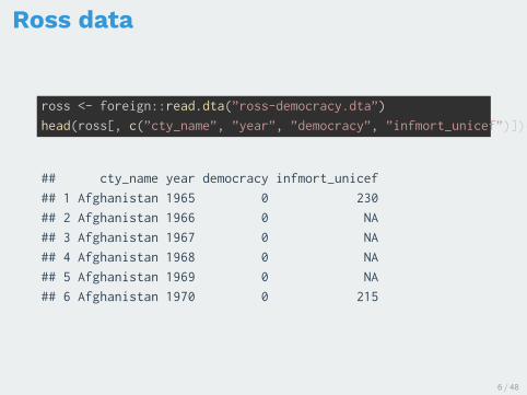
Ross data

ross <- foreign::read.dta(”ross-democracy.dta”)

head(ross[, c(”cty_name”, ”year”, ”democracy”, ”infmort_unicef”)])

## cty_name year democracy infmort_unicef

## 1 Afghanistan 1965 0 230

## 2 Afghanistan 1966 0 NA

## 3 Afghanistan 1967 0 NA

## 4 Afghanistan 1968 0 NA

## 5 Afghanistan 1969 0 NA

## 6 Afghanistan 1970 0 215

6 / 48

Pooled OLS with Ross data

pooled.mod <- lm(log(kidmort_unicef) ~ democracy + log(GDPcur),

data = ross)

summary(pooled.mod)

##

## Coefficients:

## Estimate Std. Error t value Pr(>|t|)

## (Intercept) 9.7640 0.3449 28.3 <2e-16 ***

## democracy -0.9552 0.0698 -13.7 <2e-16 ***

## log(GDPcur) -0.2283 0.0155 -14.8 <2e-16 ***

## ---

## Signif. codes: 0 ’***’ 0.001 ’**’ 0.01 ’*’ 0.05 ’.’ 0.1 ’ ’ 1

##

## Residual standard error: 0.8 on 646 degrees of freedom

## (5773 observations deleted due to missingness)

## Multiple R-squared: 0.504, Adjusted R-squared: 0.503

## F-statistic: 329 on 2 and 646 DF, p-value: <2e-16

7 / 48

Note about terminology

• Generally, we talk about panel data and time-seriescross-sectional data in political science.

• Panel data: small 𝑇 , large 𝑁▶ The NES panel is like this: 2000 respondent asked questions at

various points in time over the course of an election (ormultiple elections).

• TSCS data: high 𝑇 , low medium 𝑁 .▶ U.S. states over time▶ Western European countries over time.

• For the most part, the issues of causality are the same forthese two types of data, so I will refer to them both as paneldata.

• But estimation is a different issue. Different estimators workdifferently under either data types.

8 / 48

1/ Fixed effectsestimators

9 / 48

Notation

• Units 𝑖 = 1, … , 𝑁• Time periods 𝑡 = 1, … , 𝑇 with 𝑇 ≥ 2,• 𝑌𝑖𝑡, 𝐷𝑖𝑡 are the outcome and treatment for unit 𝑖 in period 𝑡

We have a set of covariates in each period, as well,• Covariates 𝑋𝑖𝑡, causally “prior” to 𝐷𝑖𝑡.

𝐷𝑡

𝑋𝑡

𝑌𝑡

• 𝑈𝑖 = unobserved, time-invariant unit effects (causally prior toeverything)

• History of some variable: 𝐷𝑖𝑡 = (𝐷1, … , 𝐷𝑡).• Entire history: 𝐷𝑖 = 𝐷𝑖𝑇

10 / 48

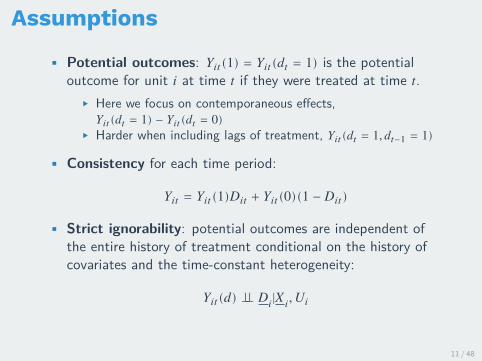
Assumptions

• Potential outcomes: 𝑌𝑖𝑡(1) = 𝑌𝑖𝑡(𝑑𝑡 = 1) is the potentialoutcome for unit 𝑖 at time 𝑡 if they were treated at time 𝑡.

▶ Here we focus on contemporaneous effects,𝑌𝑖𝑡(𝑑𝑡 = 1) − 𝑌𝑖𝑡(𝑑𝑡 = 0)

▶ Harder when including lags of treatment, 𝑌𝑖𝑡(𝑑𝑡 = 1, 𝑑𝑡−1 = 1)

• Consistency for each time period:

𝑌𝑖𝑡 = 𝑌𝑖𝑡(1)𝐷𝑖𝑡 + 𝑌𝑖𝑡(0)(1 − 𝐷𝑖𝑡)

• Strict ignorability: potential outcomes are independent ofthe entire history of treatment conditional on the history ofcovariates and the time-constant heterogeneity:

𝑌𝑖𝑡(𝑑) ⟂⟂ 𝐷𝑖|𝑋 𝑖, 𝑈𝑖

11 / 48

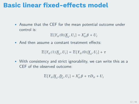
Basic linear fixed-effects model

• Assume that the CEF for the mean potential outcome undercontrol is:

𝔼[𝑌𝑖𝑡(0)|𝑋 𝑖, 𝑈𝑖] = 𝑋′𝑖𝑡𝛽 + 𝑈𝑖

• And then assume a constant treatment effects:

𝔼[𝑌𝑖𝑡(1)|𝑋 𝑖, 𝑈𝑖] = 𝔼[𝑌𝑖𝑡(0)|𝑋 𝑖, 𝑈𝑖] + 𝜏

• With consistency and strict ignorability, we can write this as aCEF of the observed outcome:

𝔼[𝑌𝑖𝑡 |𝑋 𝑖, 𝐷𝑖, 𝑈𝑖] = 𝑋′𝑖𝑡𝛽 + 𝜏𝐷𝑖𝑡 + 𝑈𝑖

12 / 48

Relating to traditional models

• We can now write the observed outcomes in a traditionalregression format:

𝑌𝑖𝑡 = 𝑋′𝑖𝑡𝛽 + 𝜏𝐷𝑖𝑡 + 𝑈𝑖 + 𝜀𝑖𝑡

• Here, the error is similar to what we had for regression:

𝜀𝑖𝑡 ≡ 𝑌𝑖𝑡(0) − 𝔼[𝑌𝑖𝑡(0)|𝑋 𝑖, 𝑈𝑖]

• In traditional FE models, we skip potential outcomes and relyon a strict exogeneity assumption:

𝔼[𝜀𝑖𝑡 |𝑋 𝑖, 𝐷𝑖, 𝑈𝑖] = 0

13 / 48

Strict ignorability vs strict exogeneity

𝑌𝑖𝑡(𝑑) ⟂⟂ 𝐷𝑖|𝑋 𝑖, 𝑈𝑖

• Easy to show to that strict ignorability implies strictexogeneity:

𝔼[𝜀𝑖𝑡 |𝑋 𝑖, 𝐷𝑖, 𝑈𝑖] = 𝔼 [(𝑌𝑖𝑡(0) − 𝔼[𝑌𝑖𝑡(0)|𝑋 𝑖, 𝑈𝑖]) |𝑋 𝑖, 𝐷𝑖, 𝑈𝑖]= 𝔼[𝑌𝑖𝑡(0)|𝑋𝑖, 𝐷𝑖, 𝑈𝑖] − 𝔼[𝑌𝑖𝑡(0)|𝑋𝑖, 𝑈𝑖]= 𝔼[𝑌𝑖𝑡(0)|𝑋𝑖, 𝑈𝑖] − 𝔼[𝑌𝑖𝑡(0)|𝑋𝑖𝑇 , 𝑈𝑖]= 0

14 / 48

Fixed-effects within estimator

• Define the “within” model:

(𝑌𝑖𝑡 − 𝑌 𝑖) = (𝑋𝑖𝑡 − 𝑋 𝑖)′𝛽 + 𝜏(𝐷𝑖𝑡 − 𝐷𝑖) + (𝜀𝑖𝑡 − 𝜀𝑖)

• Here, let 𝑌 𝑖 be the unit averages. Note that:

𝑌 𝑖 = 𝑋′𝑖𝛽 + 𝜏𝐷𝑖 + 𝑈𝑖 + 𝜀𝑖

• Logic: since the unobserved effect is constant over time,subtracting off the mean also subtracts that unobserved effect:

𝑈𝑖 − 1𝑇

𝑇∑𝑡=1

𝑈𝑖 = 𝑈𝑖 − 𝑈𝑖 = 0

• This also demonstrates why the assumption of the fixedeffects being time-constant is so important.

15 / 48

Within Estimator

• Let 𝑍𝑖𝑡 = 𝑍𝑖𝑡 − 𝑍 𝑖 be the time-demeaned version of 𝑍𝑖𝑡. Thenthe FE model is:

𝑌𝑖𝑡 = 𝑋′𝑖𝑡𝛽 + 𝜏��𝑖𝑡 + 𝜀𝑖𝑡

• Within/FE estimator, ��𝐹𝐸:pooled OLS estimator 𝑌𝑖𝑡 on 𝑋𝑖𝑡 and ��𝑖𝑡

• Only uses time variation within each cross section.• Full rank: rank[∑𝑇

𝑡=1 𝔼[ 𝑋𝑖𝑡 𝑋′𝑖𝑡]] = 𝐾

▶ Basically: no variables that are constant over time. Why?

16 / 48

Fixed effects with Ross datalibrary(plm)

fe.mod <- plm(log(kidmort_unicef) ~ democracy + log(GDPcur), data = ross,

index = c(”id”, ”year”), model = ”within”)

summary(fe.mod)

## Oneway (individual) effect Within Model

##

## Call:

## plm(formula = log(kidmort_unicef) ~ democracy + log(GDPcur),

## data = ross, model = ”within”, index = c(”id”, ”year”))

##

## Unbalanced Panel: n=166, T=1-7, N=649

##

## Residuals :

## Min. 1st Qu. Median 3rd Qu. Max.

## -0.70500 -0.11700 0.00628 0.12200 0.75700

##

## Coefficients :

## Estimate Std. Error t-value Pr(>|t|)

## democracy -0.1432 0.0335 -4.28 0.000023 ***

## log(GDPcur) -0.3752 0.0113 -33.12 < 2e-16 ***

## ---

## Signif. codes: 0 ’***’ 0.001 ’**’ 0.01 ’*’ 0.05 ’.’ 0.1 ’ ’ 1

##

## Total Sum of Squares: 81.7

## Residual Sum of Squares: 23

## R-Squared : 0.718

## Adj. R-Squared : 0.532

## F-statistic: 613.481 on 2 and 481 DF, p-value: <2e-16

17 / 48

Time-constant variables

• Pooled model with a time-constant variable, proportionIslamic:

library(lmtest)

p.mod <- plm(log(kidmort_unicef) ~ democracy + log(GDPcur) + islam, data = ross,

index = c(”id”, ”year”), model = ”pooling”)

coeftest(p.mod)

##

## t test of coefficients:

##

## Estimate Std. Error t value Pr(>|t|)

## (Intercept) 10.30608 0.35952 28.67 < 2e-16 ***

## democracy -0.80234 0.07767 -10.33 < 2e-16 ***

## log(GDPcur) -0.25497 0.01607 -15.87 < 2e-16 ***

## islam 0.00343 0.00091 3.77 0.00018 ***

## ---

## Signif. codes: 0 ’***’ 0.001 ’**’ 0.01 ’*’ 0.05 ’.’ 0.1 ’ ’ 1

18 / 48

Time-constant variables

• FE model, where the islam variable drops out, along with theintercept:

fe.mod2 <- plm(log(kidmort_unicef) ~ democracy + log(GDPcur) + islam, data = ross,

index = c(”id”, ”year”), model = ”within”)

coeftest(fe.mod2)

##

## t test of coefficients:

##

## Estimate Std. Error t value Pr(>|t|)

## democracy -0.1297 0.0359 -3.62 0.00033 ***

## log(GDPcur) -0.3800 0.0118 -32.07 < 2e-16 ***

## ---

## Signif. codes: 0 ’***’ 0.001 ’**’ 0.01 ’*’ 0.05 ’.’ 0.1 ’ ’ 1

19 / 48

Fixed-effects within estimator

• Informal proof. We have strict exogeneity:

𝔼[𝜀𝑖𝑡 |𝑋 𝑖, 𝐷𝑖, 𝑈𝑖] = 0

• This implies exogeneity of the time-averaged errors:

𝔼[𝜀𝑖|𝑋 𝑖, 𝐷𝑖, 𝑈𝑖] = 1𝑇

𝑇∑𝑡=1

𝔼[𝜀𝑖𝑡 |𝑋 𝑖, 𝐷𝑖, 𝑈𝑖] = 0

• Mean-differenced errors are uncorrelated with the treatment orregressors from any time period:

𝔼[ 𝜀𝑖𝑡 |𝑋 𝑖, 𝐷𝑖, 𝑈𝑖] = 0

• Thus, the mean-differenced treatment and covariates mustalso be uncorrelated with the mean-differenced errors:

𝔼[ 𝑌𝑖𝑡 |𝑋𝑖, 𝐷𝑖, 𝑈𝑖] = 𝑋′𝑖𝑡𝛽 + 𝜏��𝑖𝑡

20 / 48

Dummy variable regression

• An alternative way to estimate FE models is using a series ofdummy variables for each unit, 𝑖.

• Let 𝑊𝑘𝑖𝑡 = 1 if 𝑘 = 𝑖 and 𝑊𝑘

𝑖𝑡 = 0 otherwise for all 𝑘 ∈ 1, … , 𝑁 .• 𝑊𝑖𝑡 = (𝑊1

𝑖𝑡 , … , 𝑊𝑁𝑖𝑡 ) is the dummy variable vector.

• Least Squares Dummy Variable (LSDV) estimator:pooled OLS regression 𝑌𝑖𝑡 on 𝑋𝑖𝑡, 𝐷𝑖𝑡, and 𝑊𝑖𝑡.

• Algebraically equivalent to the within estimator for estimates.

21 / 48

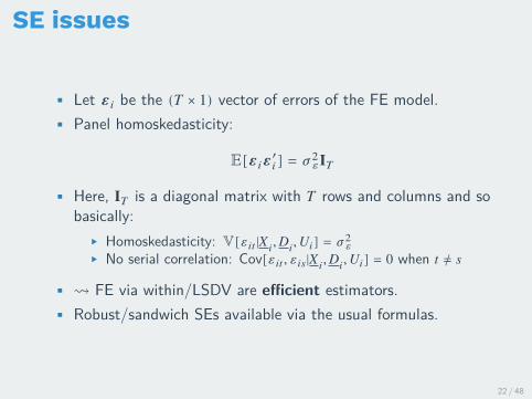
SE issues

• Let 𝜺𝑖 be the (𝑇 × 1) vector of errors of the FE model.• Panel homoskedasticity:

𝔼[𝜺𝑖𝜺′𝑖] = 𝜎2𝜀𝐈𝑇

• Here, 𝐈𝑇 is a diagonal matrix with 𝑇 rows and columns and sobasically:

▶ Homoskedasticity: 𝕍[𝜀𝑖𝑡 |𝑋 𝑖, 𝐷𝑖, 𝑈𝑖] = 𝜎2𝜀▶ No serial correlation: Cov[𝜀𝑖𝑡 , 𝜀𝑖𝑠|𝑋𝑖, 𝐷𝑖, 𝑈𝑖] = 0 when 𝑡 ≠ 𝑠

• ⇝ FE via within/LSDV are efficient estimators.• Robust/sandwich SEs available via the usual formulas.

22 / 48

Within vs LSDV

• Within estimator and LSDV give exactly the same estimates,but SEs will differ slightly.

• SEs from vanilla OLS on the within estimator will be slightlyoff due to incorrect degrees of freedom.

▶ OLS doesn’t account for you calculating the time-means.▶ Smart software (plm() in R, areg in Stata) will correct.

• LSDV estimator gets the correct SEs because time-means arecalculated by OLS ⇝ correct degrees of freedom.

▶ Downside: can be computationally demanding

23 / 48

Example with Ross data

library(lmtest)

lsdv.mod <- lm(log(kidmort_unicef) ~ democracy + log(GDPcur) + as.factor(id),

data = ross)

coeftest(lsdv.mod)[1:6, ]

## Estimate Std. Error t value Pr(>|t|)

## (Intercept) 13.76 0.266 51.8 1.0e-198

## democracy -0.14 0.033 -4.3 2.3e-05

## log(GDPcur) -0.38 0.011 -33.1 3.5e-126

## as.factor(id)AGO 0.30 0.168 1.8 7.4e-02

## as.factor(id)ALB -1.93 0.190 -10.2 4.4e-22

## as.factor(id)ARE -1.88 0.170 -11.0 2.4e-25

coeftest(fe.mod)[1:2, ]

## Estimate Std. Error t value Pr(>|t|)

## democracy -0.14 0.033 -4.3 2.3e-05

## log(GDPcur) -0.38 0.011 -33.1 3.5e-126

24 / 48

First differences

• Because the 𝑈𝑖 are time-fixed, first-differences are analternative to mean-differences.

• For some variable, 𝑍𝑖𝑡, let Δ𝑍𝑖𝑡 = 𝑍𝑖𝑡 − 𝑍𝑖,𝑡−1• The first difference model is the following:

Δ𝑌𝑖𝑡 = Δ𝑋′𝑖𝑡𝛽 + 𝜏Δ𝐷𝑖𝑡 + Δ𝜀𝑖𝑡

• This follows from the fact that Δ𝑈𝑖 = 0• By the same logic as above, strict ignorability implies strict

exogeneity which implies 𝔼[Δ𝜀𝑖𝑡 |𝑋 𝑖, 𝐷𝑖, 𝑈𝑖 = 0], so

𝔼[Δ𝑌𝑖𝑡 |𝑋 𝑖, 𝐷𝑖, 𝑈𝑖] = Δ𝑋′𝑖𝑡𝛽 + 𝜏Δ𝐷𝑖𝑡

25 / 48

First differences estimation

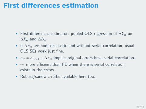
• First differences estimator: pooled OLS regression of Δ𝑌𝑖𝑡 onΔ𝑋𝑖𝑡 and Δ𝐷𝑖𝑡.

• If Δ𝜀𝑖𝑡 are homoskedastic and without serial correlation, usualOLS SEs work just fine.

• 𝜀𝑖𝑡 = 𝜀𝑖,𝑡−1 + Δ𝜀𝑖𝑡 implies original errors have serial correlation.• ⇝ more efficient than FE when there is serial correlation

exists in the errors.• Robust/sandwich SEs available here too.

26 / 48

First differences in Rfd.mod <- plm(log(kidmort_unicef) ~ democracy + log(GDPcur), data = ross,

index = c(”id”, ”year”), model = ”fd”)

summary(fd.mod)

## Oneway (individual) effect First-Difference Model

##

## Call:

## plm(formula = log(kidmort_unicef) ~ democracy + log(GDPcur),

## data = ross, model = ”fd”, index = c(”id”, ”year”))

##

## Unbalanced Panel: n=166, T=1-7, N=649

##

## Residuals :

## Min. 1st Qu. Median 3rd Qu. Max.

## -0.9060 -0.0956 0.0468 0.1410 0.3950

##

## Coefficients :

## Estimate Std. Error t-value Pr(>|t|)

## (intercept) -0.1495 0.0113 -13.26 <2e-16 ***

## democracy -0.0449 0.0242 -1.85 0.064 .

## log(GDPcur) -0.1718 0.0138 -12.49 <2e-16 ***

## ---

## Signif. codes: 0 ’***’ 0.001 ’**’ 0.01 ’*’ 0.05 ’.’ 0.1 ’ ’ 1

##

## Total Sum of Squares: 23.5

## Residual Sum of Squares: 17.8

## R-Squared : 0.246

## Adj. R-Squared : 0.244

## F-statistic: 78.1367 on 2 and 480 DF, p-value: <2e-16

27 / 48

2/ Random effects

28 / 48

Random effects

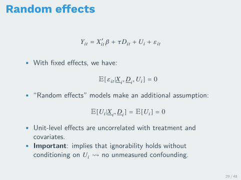
𝑌𝑖𝑡 = 𝑋′𝑖𝑡𝛽 + 𝜏𝐷𝑖𝑡 + 𝑈𝑖 + 𝜀𝑖𝑡

• With fixed effects, we have:

𝔼[𝜀𝑖𝑡 |𝑋 𝑖, 𝐷𝑖, 𝑈𝑖] = 0

• “Random effects” models make an additional assumption:

𝔼[𝑈𝑖|𝑋𝑖, 𝐷𝑖] = 𝔼[𝑈𝑖] = 0

• Unit-level effects are uncorrelated with treatment andcovariates.

• Important: implies that ignorability holds withoutconditioning on 𝑈𝑖 ⇝ no unmeasured confounding.

29 / 48

Why random effects?

• So why do people use random effects? Standard errors!• Under the RE assumption, we have the following:

𝑌𝑖𝑡 = 𝑋′𝑖𝑡𝛽 + 𝜏𝐷𝑖𝑡 + 𝜈𝑖

where 𝜈𝑖 = 𝑈𝑖 + 𝜀𝑖𝑡.• Now, notice that

cov[𝑌𝑖1, 𝑌𝑖2|𝑋 𝑖𝑡 , 𝐷𝑖𝑡] = 𝜎2𝑢

where 𝜎2𝑢 is the variance of the 𝑈𝑖.• This violates the assumption of no autocorrelation for OLS.

What’s the problem with this?• Random effects models gets us consistent standard error

estimates.

30 / 48

Quasi-demeaning

• Random effects models usually transform the data via what iscalled quasi-demeaning or partial pooling:

(𝑌𝑖𝑡 − 𝜃𝑌 𝑖) = (𝑋𝑖𝑡 − 𝜃𝑋 𝑖)′𝛽 + 𝜏(𝐷𝑖𝑡 − 𝜃𝐷𝑖) + (𝜈𝑖𝑡 − 𝜃𝜈𝑖)

• Here 𝜃 is between zero and one, where 𝜃 = 0 implies pooledOLS and 𝜃 = 1 implies fixed effects. Doing some math showsthat

𝜃 = 1 − [𝜎2𝑢/(𝜎2𝑢 + 𝑇𝜎2𝜀)]1/2

• the random effect estimator runs pooled OLS on this modelreplacing 𝜃 with an estimate 𝜃.

31 / 48

Example with Ross datare.mod <- plm(log(kidmort_unicef) ~ democracy + log(GDPcur), data = ross,

index = c(”id”, ”year”), model = ”random”)

coeftest(re.mod)[1:3, ]

## Estimate Std. Error t value Pr(>|t|)

## (Intercept) 12.31 0.255 48.3 1.6e-216

## democracy -0.19 0.034 -5.6 2.4e-08

## log(GDPcur) -0.36 0.011 -32.8 1.5e-139

coeftest(fe.mod)[1:2, ]

## Estimate Std. Error t value Pr(>|t|)

## democracy -0.14 0.033 -4.3 2.3e-05

## log(GDPcur) -0.38 0.011 -33.1 3.5e-126

coeftest(pooled.mod)[1:3, ]

## Estimate Std. Error t value Pr(>|t|)

## (Intercept) 9.76 0.345 28 2.9e-115

## democracy -0.96 0.070 -14 1.2e-37

## log(GDPcur) -0.23 0.015 -15 1.2e-42

• More general random effects models using lmer() from thelme4 package

32 / 48

Hausman tests

• Can we test the assumption that 𝔼[𝑈𝑖|𝑋 𝑖, 𝐷𝑖] = 𝔼[𝑈𝑖]?▶ If true (and all the RE assumptions hold), then RE and FE are

consistent, but RE is efficient.▶ If false, then RE is inconsistent, but FE is consistent.

• A Hausman test uses these facts to develop a hypothesis testof the assumption:

▶ If FE and RE estimates are similar ⇝ assumption plausible.▶ If FE and RE very different ⇝ assumption perhaps not

plausible.• Limitations:

1. We must maintain strict exogeneity for null and alternative.2. Must maintain that 𝑈𝑖 is homoskedastic (not required for FE)3. Limited to comparing coefficients on variables that vary in 𝑖

and 𝑡.

33 / 48

Calculate the Hausman test

• Let 𝑆𝐸[��𝐹𝐸] and 𝑆𝐸[��𝑅𝐸] be the estimated SEs of theestimators.

▶ Under the null that RE is correct, 𝑆𝐸[��𝐹𝐸] > 𝑆𝐸[��𝑅𝐸]

• Hausman test statistic:

𝐻 = ��𝐹𝐸 − ��𝑅𝐸

(𝑆𝐸[��𝐹𝐸]2 − 𝑆𝐸[��𝑅𝐸]2)1/2

• Under the null hypothesis that RE is correct, 𝐻 isasymptotically normal.

• When ��𝐹𝐸 and ��𝑅𝐸 are very different relative to theiruncertainty, 𝐻 will be big in absolute value and we will rejectthe null.

34 / 48

Hausman test in R

phtest(fe.mod, re.mod)

##

## Hausman Test

##

## data: log(kidmort_unicef) ~ democracy + log(GDPcur)

## chisq = 70, df = 2, p-value = 8.041e-16

## alternative hypothesis: one model is inconsistent

35 / 48

3/ Fixed effects withheterogeneoustreatment effects

36 / 48

Potential outcomes in the generalsetting

• Let’s allow for heterogenerous treatment effects:

𝜏𝑖𝑡 = 𝑌𝑖𝑡(1) − 𝑌𝑖𝑡(0)

• Keeping the old linearity in 𝑋𝑖𝑡 assumption:

𝑌𝑖𝑡 = 𝑋′𝑖𝑡𝛽 + 𝜏𝑖𝑡𝐷𝑖𝑡 + 𝑈𝑖 + 𝜀𝑖𝑡

• Add and substract 𝜏𝐷𝑖𝑡, where 𝜏 = 𝔼[𝜏𝑖𝑡]:

𝑌𝑖𝑡 = 𝑋′𝑖𝑡𝛽 + 𝜏𝐷𝑖𝑡 + 𝑈𝑖 + 𝜂𝑖𝑡

• Where the combined error is:

𝜂𝑖𝑡 = (𝜏𝑖𝑡 − 𝜏)𝐷𝑖𝑡⏟⏟⏟⏟⏟non-constant effects

+ 𝑌𝑖𝑡(0) − 𝐸[𝑌𝑖𝑡(0)|𝑋 𝑖, 𝑈𝑖]⏟⏟⏟⏟⏟⏟⏟⏟⏟⏟⏟typical errors, 𝜀𝑖𝑡

37 / 48

Assumptions

• Earlier we showed that strict ignorability implied strictexogeneity for 𝜀𝑖𝑡. What about 𝜂𝑖𝑡?

𝔼[𝜂𝑖𝑡 |𝑋 𝑖, 𝐷𝑖, 𝑈𝑖] = 0

• Since 𝜂𝑖𝑡 = (𝜏𝑖𝑡 − 𝜏)𝐷𝑖𝑡 + 𝜀𝑖𝑡 and we showed that𝔼[𝜀𝑖𝑡 |𝑋𝑖, 𝐷𝑖, 𝑈𝑖] = 0, it suffices to show:

𝔼[(𝜏𝑖𝑡 − 𝜏)𝐷𝑖𝑡 |𝑋 𝑖, 𝐷𝑖, 𝑈𝑖] = 0

38 / 48

Non-constant effects errors

• How does the non-constant effect error work here?

𝔼[(𝜏𝑖𝑡 − 𝜏)𝐷𝑖𝑡 |𝑋𝑖, 𝐷𝑖, 𝑈𝑖] = 𝐷𝑖𝑡(𝔼[𝜏𝑖𝑡 − 𝜏|𝑋 𝑖, 𝐷𝑖, 𝑈𝑖])= 𝐷𝑖𝑡(𝔼[𝜏𝑖𝑡 |𝑋 𝑖, 𝐷𝑖, 𝑈𝑖] − 𝜏)= 𝐷𝑖𝑡(𝔼[𝜏𝑖𝑡 |𝑋 𝑖, 𝑈𝑖] − 𝜏)= 𝐷𝑖𝑡(𝔼[𝜏𝑖𝑡 |𝑋 𝑖, 𝑈𝑖] − 𝔼[𝜏𝑖𝑡])

• Thus, we can see that the combined error will only satisfy thestrict exogeneity assumption of fixed effects when

𝐸[𝜏𝑖𝑡 |𝑋 𝑖, 𝑈𝑖] = 𝐸[𝜏𝑖𝑡]

• This is when the treatment effects are independent of the uniteffects and the covariates.

39 / 48

Regression bias?

• We’ve seen this before: it’s a general problem with regressionand varying treatment effects.

𝜂𝑖𝑡 = 𝐷𝑖𝑡(𝜏𝑖𝑡 − 𝜏)⏟⏟⏟⏟⏟non-constant effects

+ 𝑌𝑖𝑡(0) − 𝐸[𝑌𝑖𝑡(0)|𝑋 𝑖, 𝑈𝑖]⏟⏟⏟⏟⏟⏟⏟⏟⏟⏟⏟typical errors

• Generally the issue here is that non-constant effects inducecorrelation between the treatment and the error term.

• Distinct from confounding bias since we could, in principle,estimate 𝐸[𝜏𝑖𝑡 |𝑋 𝑖, 𝑈𝑖] to then calculate 𝐸[𝜏𝑖𝑡]

• Overall ATE still nonparametrically identified, even if the FEregression doesn’t estimate it.

40 / 48

Strict exogeneity/ignorability

𝑌𝑖𝑡(𝑑) ⟂⟂ 𝐷𝑖|𝑋 𝑖, 𝑈𝑖

• Strict ignorability is very strong.• Rules out the following:

▶ 𝐷𝑖𝑡 affects 𝑌𝑖𝑡 which then affects 𝐷𝑖,𝑡+1▶ Basically, any feedback between treatment and the outcome

• Can we weaken this? Yes! Sequential ignorability:

𝑌𝑖𝑡(𝑑) ⟂⟂ 𝐷𝑖𝑡 |𝑋 𝑖𝑡 , 𝐷𝑖,𝑡−1, 𝑈𝑖

• Note here that the we only condition up to 𝑡 so that the errorscan be correlated with future 𝐷𝑖,𝑡+1 and so on.

• This implies sequential exogeneity of the errors:

𝔼[𝜀𝑖𝑡 |𝑋𝑖𝑡 , 𝐷𝑖𝑡 , 𝑈𝑖] = 0.

41 / 48

Strict ignorability example

• Example: economic interdependence between countries(𝐷𝑖𝑡 = 1 if county-dyad 𝑖 is interdependent in period 𝑡) andconflict severity (𝑌𝑖𝑡) between countries.

• Strict ignorability assumption implies shocks to conflictseverity at 𝑡 uncorrelated with:

▶ future values of conflict severity▶ economic interdendence▶ any other time-varying covariate

42 / 48

Lagged dependent variables

𝑌𝑖𝑡 = 𝛽𝑌𝑖,𝑡−1 + 𝜏𝐷𝑖𝑡 + 𝑈𝑖 + 𝜀𝑖𝑡

• Fixed effects models with lagged dependent variables is muchharder.

• Easiest to see with first differences:

(𝑌𝑖𝑡 − 𝑌𝑖,𝑡−1) = 𝛽(𝑌𝑖,𝑡−1 − 𝑌𝑖,𝑡−2) + 𝜏(𝐷𝑖𝑡 − 𝐷𝑖,𝑡−1) + (𝜀𝑖𝑡 − 𝜀𝑖,𝑡−1)

• Obviously, 𝑌𝑖,𝑡−1 is correlated with the 𝜀𝑖,𝑡−1.• This is sometimes called a dynamic panel model, where we

can’t rely on the exogeneity assumption alone.• ⇝ need an instrumental variable approach (coming up in a

few weeks).

43 / 48

4/ Cumulative effects

44 / 48

Contemporaneous vs Cumulative effects

• Another assumption we’ve been making is that there is only acontemporaneous effect: 𝜏𝐷𝑖𝑡.

• Implicitly or explicitly fixing the past history of the treatment.• What if we want to estimate the cumulative effects?• Very difficult, if not impossible with fixed effects models.• Why?

▶ For cumulative effects, we need to consider the effects oftreatment on time-varying confounders, 𝑋𝑖𝑡(𝑑𝑖,𝑡−1).

▶ Those pathways might be hard to identify

45 / 48

New notation

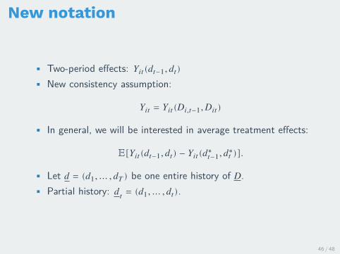
• Two-period effects: 𝑌𝑖𝑡(𝑑𝑡−1, 𝑑𝑡)• New consistency assumption:

𝑌𝑖𝑡 = 𝑌𝑖𝑡(𝐷𝑖,𝑡−1, 𝐷𝑖𝑡)

• In general, we will be interested in average treatment effects:

𝔼[𝑌𝑖𝑡(𝑑𝑡−1, 𝑑𝑡) − 𝑌𝑖𝑡(𝑑∗𝑡−1, 𝑑∗𝑡 )].

• Let 𝑑 = (𝑑1, … , 𝑑𝑇 ) be one entire history of 𝐷.• Partial history: 𝑑𝑡 = (𝑑1, … , 𝑑𝑡).

46 / 48

Fixed effects causal models

• Need a causal model:

𝑌𝑖𝑡(𝑑𝑡−1, 𝑑𝑡) = 𝑋′𝑖𝑡(𝑑𝑡−1)𝛽𝑐 + 𝜏𝑖,𝑡−1𝑑𝑡−1 + 𝜏𝑖𝑡𝑑𝑡 + 𝑈𝑖 + 𝜀𝑖𝑡

• 𝛽𝑐 have 𝑐 subscript here to denote difference from above fixedeffect regressions.

• Allows for heterogeneous effects in each unit-period.

𝔼[𝑌𝑖𝑡(1, 1) − 𝑌𝑖𝑡(0, 0)] = 𝔼[𝜏𝑖,𝑡−1 + 𝜏𝑖𝑡⏟⏟⏟⏟⏟direct effects

+ (𝑋𝑖𝑡(1) − 𝑋𝑖𝑡(0))′𝛽𝑐⏟⏟⏟⏟⏟⏟⏟⏟⏟effect of 𝐷𝑖,𝑡−1 through 𝑋𝑖𝑡

]

47 / 48

Cumulative effects notes

• Sobel paper shows that under fixed effects-style confoundingcan only estimate contemporaneous effect, where 𝑑𝑡−1 is thesame for the comparison:

𝔼[𝑌𝑖𝑡(𝑑𝑡−1, 1) − 𝑌𝑖𝑡(𝑑𝑡−1, 0)] = 𝔼[𝜏𝑖𝑡]

• 𝛽𝑐 is very difficult to identify! Need more restrictions.• Exception: 𝑋𝑖𝑡 is unaffected by 𝐷𝑖,𝑡−1 so that 𝑋𝑖𝑡(1) = 𝑋𝑖𝑡(0)

and so:

𝔼[𝑌𝑖𝑡(1, 1) − 𝑌𝑖𝑡(0, 0)] = 𝔼[𝜏𝑖,𝑡−1 + 𝜏𝑖𝑡]

48 / 48