Governance and Economic Development: Good Governance and Millennium Development Goals Yashar Tarverdimamaghani This thesis is presented for the degree of Doctor of Philosophy of University of Western Australia UWA Business School Economics 2015
Transcript
Governance and Economic Development:
Good Governance and Millennium Development Goals
Yashar Tarverdimamaghani
This thesis is presented for the degree of
Doctor of Philosophy of
University of Western Australia
UWA Business School
Economics
2015
ii
i
Abstract This study examined whether the Good Governance (Boeninger, 1991) reforms
recommended by the World Bank have been successful in helping countries to achieve
the United Nation’s (UN) Millennium Development Goals (MDGs) implemented in
2000 to encourage development by improving the socioeconomic conditions of the
world’s poorest countries (Raykar, 2011; UN, 2000).
In this study, a new methodology was developed for the construction of a
new governance indicator. This new methodology extended Goldberger’s (1972)
Multiple Indicators Multiple Cause (MIMC) methodology. This study used the
‘raw’ data of Kaufmann et al.’s (1999) and a simulation study to compare the
results of the new methodology with Kaufmann’s (1999) methodology. The new
methodology was found to deliver a better governance indicator with higher
precision and lower variance.
To enable more in-depth research to be undertaken, the scope of this study
was limited to an examination of a number of carefully selected MDGs.
Specifically, this study examined the effect of governance and health aid on child
mortality rates and found that governance has an important role in reducing child
mortality rates. Additionally, this study considered the environmental aspect of the
MDGs, CO2 emissions, and found that while governance as a whole has a
statistically significant role in reducing Carbon Dioxide (CO2) emissions, Control
of Corruption (CC) has a much larger role in reducing CO2 emissions. The role of
CC on CO2 emissions was found to be robust across different models and
methodologies. Overall, the findings suggested that levels of governance are
deterministic in achieving the MDGs. Thus, Good Governance should be
considered as strategy for achieving MDGs.
iii
Contents Abstract ................................................................................................... i
Contents ................................................................................................. iii
List of Tables ........................................................................................ vii
List of Figures ....................................................................................... ix
List of Abbreviations ............................................................................ xi
Certificate of Authorship/Originality ................................................. xv
Dedication .......................................................................................... xvii
Acknowledgements ............................................................................. xix
2.2.2 The World Governance Indicators Methodology versus the Goldberger Methodology ................................................................................................................. 16
2.2.3 The Proposed Methodology ........................................................................... 16
Santiso et al., 2001). Consequently, the importance of the WGIs also increased and,
10
since then, the WGIs have been used in many areas of research as a main measure of
governance.
However, despite their popularity, the WGIs have been subject to criticism (Al-
Marhubi, 2004; Langbein & Knack, 2010), as their specifications have been found to
restrict their application in researches and have also affected the results of several
studies (Langbein & Knack, 2010). The existence of lower and upper bands in the
results makes cross-country or cross-aspect comparisons and panel data analysis
challenging. Further, it appears that these bands could overlap across countries, thus
making the identification of any improvements or declines in governance impossible.
Kaufman et al. (1999) raised this very issue also, which can be clarified if the following
two scenarios are considered:
1- Country X has indicator 3 with the upper band value 5 and a lower band
value of 1.
2- Country Y has indicator 2 with upper band values of 5.5 and a lower
band value of and 1.5.
Any comparison between the above two cases is almost impossible, as the values for
each case could vary between the upper and lower bands. Thus, the application of the
WGIs is limited to a time series.
Langbein and Knack (2010) asserted that the WGIs have a number of conceptual
and technical issues. In the following sections, criticisms of the WGIs and the
implications of these criticisms are discussed. Langbein and Knack’s (2010) criticisms
are the most significant, as they point out that the inadequacies of the WGIs from
different perspectives.
The importance and benefit of having a single index that measures governance for
the purposes of policy decisions and research projects was mentioned above. In this
11
study, a new methodology was proposed with the aim of constructing a governance
indicator that accommodates the conceptual characteristics of governance. This new
methodology was designed to addresses some of the criticisms directed at the WGIs.
Additionally, it extended the existing Multiple Indicators Multiple Cause (MIMC)
methodology.
In the next section, the methodology that Kaufmann et al. (1999) used to develop
the WGIs is reviewed. Next, criticisms and limitations of the methodology are
considered. Following this, a new methodology and model are proposed. An
explanation is given of how this new methodology responds to criticisms directed at the
WGIs and overcomes the limitations of the WGIs. The results are then set out and a
new governance indicator is constructed to demonstrate how the new methodology can
be applied. A robustness check is undertaken with the same ‘raw’ data used in the
original set and the WGIs are reproduced to show the differences in results between the
WGIs and the new methodology. The results of a simulation study are then presented.
The results confirmed that the new methodology is more efficient than WGIs
methodology. In the final section, the results of the methodology and possible
applications of the proposed methodology are discussed.
2.1.1 The World Bank’s Methodology
As stated above, the ‘Good Governance’ concept identifies eight aspects of good
governance; however, in developing the WGIs, Kaufmann et al. (1999) reduced these
eight aspects to six. To create indicators, Kaufmann et al. (1999) considered groups of
sub-indicators that represented six aspects of governance.2 For each group, they
assumed that any individual data source provides an imperfect signal of some deeper
underlying notion of governance that may be difficult to observe directly. Thus,
2 See Appendix 6.3, a part of this grouping is presented as an example.
12
Kaufmann et al. (1999) assumed that each of the existing sub-indicators followed an
equation such as:
𝑦𝑛,𝑖 = 𝛼𝑖 + 𝛽𝑖(𝑦𝑛∗ + 𝜖𝑛,𝑖) , 𝜖𝑛,𝑖 ∼ 𝑁(0, 𝜎𝑖
2) (2.1)
In which:
- and are the parameters;
- is the unobserved governance in country and 𝑦𝑛∗ ∼ 𝑁(0,1);
- is observed score of country n on indicator i; and
- E[ϵn,i, ϵn,j] = 0 𝑖𝑓 𝑖 ≠ 𝑗
Based on equation (2.1), the contribution to the log likelihood function by country
𝑛 is:
𝑙(𝜶, 𝜷, 𝝈𝟐)𝑛 ∝ ln|Ω| + (𝒚𝒏 − 𝜶)′Ω−1
(𝒚𝒏 − 𝜶) (2.2)
In which:
- ;
- is a vector of 𝐼 × 1 indicators for country ;
- , , ; and
- and are diagonal matrices with 𝛽𝑖 and in the diagonal.
For each six group of WGIs, Kaufmann et al. (1999) found Maximum Likelihood (ML)
estimates of and , then calculated the conditional expected value and the conditional
variance of governance aspect with the equations as follows:
𝐸[𝑦𝑛
∗|𝑦𝑛,1, … . , 𝑦𝑛,𝐼] = ∑ 𝑤𝑖
𝑦𝑛,𝑖 − 𝛼𝑖
𝛽𝑖
𝐼
𝑖=1
(2.3)
In which:
- is the weight that depends inversely on the variance of error
term; and
- 𝑦𝑛,𝑖−𝛼𝑖
𝛽𝑖 is the score of governance for each country.
13
The equation (2.3) is simply a weighted average of scores for each country. The
conditional standard deviation of 𝑦𝑛∗, which indicates the precision of the estimated
indicator, is:
𝑆. 𝐷. 3[𝑦𝑛∗|𝑦𝑛,1, … . . 𝑦𝑛,𝐼] = (1 + ∑ 𝜎𝑖
2
𝐼
𝑖=1
)
−12
(2.4)
As stated above, Langbein and Knack (2010) have asserted that the widespread
use of the WGIs might have significantly misled many policy makers and researchers.
The criticisms made by Langbein and Knack (2010) relate to the:
1. Strong correlation among the WGIs: Langbein and Knack (2010) argue that the
strong correlations between the six WGIs indicate that the WGIs measure one
single concept rather than six different aspects of one concept.
2. Initial Grouping: Langbein and Knack (2010) state that there was no basis for
the grouping of the indicators used to generate the WGIs. Further, they assert
that Kaufmann et al. (1999) failed to provide any scientific support for the
grouping of the sub-indicators and that in categorising the initial indicators a
proven and cited hypothesis4 should have been used for the grouping, as it
would have revealed how the sub-indicators were related.
3. Methodology: Langbein and Knack (2010) contend that Kaufmann‘s
methodology failed to distinguish between causal, measurement and mixed
models.
4. Complexity: Langbein and Knack (2010) argue that methodology of the WGIs is
overly complicated and difficult for non-econometricians to interpret.
3 Standard Deviation. 4 Langbein and Knack (2010) argued that the initial grouping should have been based on cited research and well-referenced, well-established literature.
14
In the following section, a new methodology is proposed. It is then explained how
this new methodology addresses some of the aforementioned criticisms.
2.2 Methodology and Model
In this study, it was theorised that the issues related to the initial groupings and
the strong correlations between the different indictors could be avoided by aggregating
the existing indicators into one single indicator.
To address debates on the choice of an appropriate methodology, the advantages
and disadvantages of some known aggregation methods were considered (see
Appendix 6.4). The following section sets out why Goldberger’s (1972) methodology,
known as the MIMC methodology, is a more appropriate measure of unobservable
concepts such as governance. Three reasons support this choice:
1. The initial methodology proposed by Goldberger (1972) is fundamentally
about an unobservable concept (similar to governance).
2. Compared to other discussed methodologies, the MIMC methodology
allows the existence of error terms to be associated with each indicator.
3. In the MIMC methodology there is no specific requirement related to the
indicators used in the model unlike in other methodologies such as PCA.
In the next section, the basis of the MIMC methodology is examined in greater
detail and similarities to Kaufmann et al.’s (1999) UCM are noted. The foundations of
the methodology used in this study are also explained.
2.2.1 Goldberger’s Methodology
To construct the new aggregate indicator, the methodology pioneered by
Goldberger (1972) and further developed by Jöreskog and Goldberger (1975) was used.
Goldberger (1972) assumed that is an unobserved (latent) variable and that a vector
15
of some exogenous variables (X) has an equation such as that provided by
equation (2.5). Goldberger (1972) also assumed that the vector of indicators Y,
measures imperfectly (see equation (2.6)). The vector of U in equation (2.6)
includes the relative measurement or methodological errors.
(2.5)
(2.6)
In which:
- , , ;
- , , ;
- , , ; and
- is an m × m diagonal matrix with (i.e., the vector of standard deviation of
the u’s) displayed on its diagonal.
Goldberger (1972) showed that parameters could be estimated using the
Maximum Likelihood (ML). Goldberger (1972) named X as the vector of Multiple
Causes and Y as the vector of Multiple Indicators. Thus, this methodology was named
the MIMC methodology.
16
2.2.2 The World Governance Indicators Methodology versus the Goldberger Methodology
Comparing the methodology used by Kaufmann et al. (1999) with Goldberger’s
(1972) methodology, two main differences can be identified. First, in Kaufmann et al.’s
(1999) econometrical definition, governance is an unobservable stochastic variable.
This assumption means equation (2.5) can be written as:5
Second, Kaufmann et al. (1999) introduced a vector of to capture differences
in scales. However, in Goldberger’s (1972) methodology there was an underlying
assumption that the indicators had the same scales.
2.2.3 The Proposed Methodology
In the new methodology, similar to Kaufmann et al.’s (1999) methodology, it was
assumed that each of the existing indicators gives a biased picture of unobserved
governance. It was also assumed that the unobserved governance ( ) is a random
variable that follows a normal distribution with a mean of 0 and variance of 1. Given
this definition, can be written as:
(2.7)
In which, is scalar and is different for each of the observations (countries) at any
given time6 and its variance is 1 (i.e., ). Equation (2.7) can also be written as:
(2.8)
5 Kaufman et al. (1999) did not set out the underlying assumptions of the definition or their reasons for not including a vector of X in the model. However, there may be a few reasons for the vector of X being omitted from their model of governance indicators. Ideally, the vector of X should include variables that may cause changes in governance (y*), but as this branch of literature is still relatively young and there is no scientific consensus, generating indicators omitting the vector of X seems practical. 6 Where is a random variable that is normally distributed across countries for any given year.
17
It was then assumed that each of the governance indicators for a country provides a
biased picture of the unobserved 𝑦∗. Thus, the equivalent equation would be:
(2.9)
In which:
- is the indicator for country ;
- is the parameter that controls different scales in indicator ;
- is the parameter that maps the unobserved into the observed .; and
- represents any measurement or methodological error associated with the
observed indicator ( ) and country .7
In Equation (2.9), similar to Kaufmann et al.’s (1999) methodology, is introduced to
cover the different scale in , as each of the observed indicators has its own
measurement scale.
It should be noted that in Goldberger’s (1972) basic MIMC model, which
included an assumption of an I observed indicator for each country, there is no vector of
. A possible underlying assumption of the Goldberger (1972) model is
that all the indicators measuring the unobserved concept have the same scales or could
be normalised to have the same scales. Thus, if normalised indicators are considered in
, the vector of α can be ignored and the equation (2.9) changed to:
(2.10)
It is apparent that , , are different to their counterparts in equation (2.9).
However, the result (i.e., the estimation of 𝑦∗) would not be any different. In this study,
to keep the model as generic as possible, the vector of is also included to account for
different scales of indicators in
7 In further equations, the assumptions regarding are presented and explained.
18
As in equation (2.6), one of the fundamental assumptions of Kaufmann et al.’s
(1999) model is that the Us are independent. Such an assumption implies that each of
the observed indicators has their own unique measurement and methodological error
that is not correlated with the error term of other indicators. This is an unrealistic
assumption, as an error associated with one indicator that measures a specific aspect
could be correlated with another indicator’s error term. Relaxing this assumption
implies that:
.
It appears that the correlation between the results of the WGIs was partially
caused by the fact that Kaufmann et al. (1999) failed to account for the high possible
overlap between errors of individual indicators. Relaxing the assumption of independent
error terms allows the variance-covariance matrix of U (error terms) to have both
diagonal and off-diagonal elements. It was tempting to consider an unstructured
variance-covariance matrix and estimate all the elements in the matrix; however, this
was not computationally possible. A problem arose because, after combing two
equations and creating the reduced form, multiplication of parameters of appeared in
all (i.e., both diagonal and off-diagonal) of the variance-covariance matrix alongside the
s. This made the estimation impossible; thus, it was necessary to restrict variance-
covariance matrix.8
8 It should be noted that there were no problems of incidental parameters (as mentioned by Vinod (2008)). In this set-up, the number of observations (i.e., countries) was much larger than the number of unknown parameters (i.e., the length of β or the number of observed indicators). However, a problem appeared in a reduced form when multiplication of out of interest parameters of different 𝛽s with various 𝜎 (i.e., 𝛽𝑖𝛽𝑧𝜎𝑖𝜎𝑧) equalled a single element of the variance-covariance matrix. Consequently, estimating the elements of the variance covariance matrix when they consist of multiplication of the out of interest parameters is impossible. Goldberger (1972) also mentioned this issue. In this method, the multiplications of the parameters appear in all derivatives of MLE; thus, it is not possible to solve the function unless the parameters are restricted. Again, Goldberger (1975) mentioned this issue (and see the first footnote of Goldberger’s article). Further, no problem originates from the number of unknown parameters in this model, as the use of at least 100 countries and 11 indicators means that the unstructured variance covariance matrix would be 11 x 11 and would have at most 121 parameters (fully
19
However, restricting the covariance matrix required knowledge of possible
relationships between error terms, which was also not possible, as the governance is
unobservable as are the error terms associated with its measurement. As a solution to
this problem, the indicators were clustered to reduce the number of parameters to be
estimated in off-diagonal elements of the variance-covariance matrix. By clustering
indicators, it is assumed that for each cluster any measurement error includes a random
variable and noise that is unique to each indicator and has a normal distribution with a
zero mean and variance of .
(2.11)
(2.12)
Combining equations (2.11) and (2.9), the main equation can be rewritten as:
(2.13)
In equation (2.13), the is the random variable (effect) associated with cluster .
The random variables were introduced based on the idea of random effects in panel data
analysis.9 Given the fact that there might be several clusters in the dataset and
considering the matrix of observed I indicators for n countries, the matrix representation
of the equation (2.13) is derived as:
(2.14)
In which:
- is a vector of 1;
unconstructed case) and on the other side of the regression (equation) there are 100 x 11 = 1,100 elements. Thus, the number of equations is far larger than number of parameters. 9 It might be conceptually easier if equation (2.13) was viewed from a different perspective and as a model in the panel data. Then, the 𝛼𝑖 could be viewed as a time effect and 𝜉𝑛 could be viewed as a random effect; these notations would make the model similar to a mixed model panel data.
20
- if and ;
- ;
- ; and
- is a diagonal matrix of on its diagonal.
Based on equation (2.8), the conditional distribution of observed on could be
written as:
(2.15)
In which:
- is the square matrix that has a number of partitions equal to the number of
clusters;
- = ; and
- .
From equation (2.15), and following the specifications of normal distribution, the
marginal distribution of is:
(2.16)
In which:
(2.17)
Further, based on (2.15), , equation (2.18) can be changed to:
For the purpose of finding an indicator for unobserved variables, , similar to
Goldberger (1972) and Kaufmann et al. (1999), the expected value of the unobserved
governance in condition to the observed vector of (i.e. ) could be used. To
21
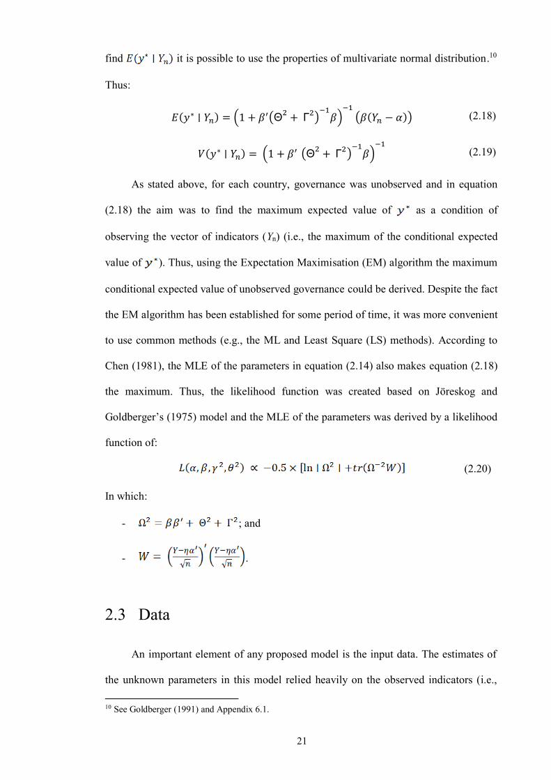
find it is possible to use the properties of multivariate normal distribution.10
Thus:
𝐸(𝑦∗ ∣ 𝑌𝑛) = (1 + 𝛽′(Θ
2+ Γ2)
−1𝛽)
−1
(𝛽(𝑌𝑛 − 𝛼)) (2.18)
𝑉(𝑦∗ ∣ 𝑌𝑛) = (1 + 𝛽′ (Θ
2+ Γ
2)−1
𝛽)−1
(2.19)
As stated above, for each country, governance was unobserved and in equation
(2.18) the aim was to find the maximum expected value of as a condition of
observing the vector of indicators (Yn) (i.e., the maximum of the conditional expected
value of ). Thus, using the Expectation Maximisation (EM) algorithm the maximum
conditional expected value of unobserved governance could be derived. Despite the fact
the EM algorithm has been established for some period of time, it was more convenient
to use common methods (e.g., the ML and Least Square (LS) methods). According to
Chen (1981), the MLE of the parameters in equation (2.14) also makes equation (2.18)
the maximum. Thus, the likelihood function was created based on Jöreskog and
Goldberger’s (1975) model and the MLE of the parameters was derived by a likelihood
function of:
(2.20)
In which:
- ; and
- .
2.3 Data
An important element of any proposed model is the input data. The estimates of
the unknown parameters in this model relied heavily on the observed indicators (i.e., 10 See Goldberger (1991) and Appendix 6.1.
22
the Y matrix). In this model, 11 indicators measuring different aspects of governance
were used. These indicators covered almost 116 countries for the period of 2012 to
2013 (see Table 2.1).
The same data used by Kaufmann et al. (1999) to construct the WGIs was
accessed for this study. There were almost 30 indicators within this official source of
data for the WGIs; however, not all of the indicators had good coverage across the
countries. Thus, a culling of the indicators was inevitable. In this study, the indicators
that covered a relatively large number of countries11 were selected. This restriction
reduced the number of indicators used to 11. However, using the same data source as
that used for the WGIs provided an important advantage; that is, it increased the
comparability of the results of the two methods. The selected indicators from the WGI
website had been normalised across all the countries;12 thus, there was no need to
consider vector and the main equation used was (2.10).
One of the major differences between the proposed methodology and that used
for the WGIs is the introduction of clusters in the covariance matrix. The introduction
of clusters relaxed the assumption of the independent error terms. Thus, the number of
clusters and the way they are created plays a crucial role in the estimation. However, it
was recognised that clustering the variables based on any ad-hoc practice could create
issues. Accordingly, in this study, the indicators and their error terms were clustered
around the initial grouping used by Kaufmann et al. (1999) to create their six indicators.
By way of example, Kaufmann et al. (1999) believed that the Freedom House
Democracy Index (FRH) and Reporters without Borders Press Freedom Index (RSF)
provided information on democratic aspects of governance; thus, these indexes were
aggregated for VA and included as one cluster. 11 Any indicator that covered more than 85 per cent of the official World Bank list of countries was used. This selection made it possible to address an issue the basic method; that is, its high dependency on used data. 12 They all had an average of zero and a standard deviation close to 1, ranging from -2.5 to 2.5.
23
As stated above, Kaufman et al.’s (1999) initial groupings have been criticised.
Thus, the use of this categorisation in clustering could create issues; however, the same
grouping was maintained to ensure comparable results were produced. Further, while
the initial groupings of indicators by Kaufman et al. (1999) has been the subject of
debate, adopting the same grouping for error terms was reasonable, as there was a high
probability that the error terms associated with the conceptually close indicators would
be correlated. Further, before any ‘official’ indicator can be constructed, more research
is required and more comprehensive and well-established categories are needed.
It was assumed that the measurement errors of indicators in one cluster would
correlate with the same ratio, but be independent of, the error terms in other clusters. In
Table 2.1, the indicators are presented along with their clusters.
Table 2.1: Clusters of Indicators used in Creating the New GI
No Indicator Description Clusters
1 FRH Freedom House Democracy Index 1
2 RSF Reporters Without Borders Press Freedom Index 3 HER Heritage Foundation Index of Economic Freedom 2
4 TPR US State Department Trafficking in People Report 5 Ijt iJET Country Security Risk Ratings 3
6 HUM Cingranelli Richards Human Rights Database 4
7 IPD Institutional Profiles Database 8 PRS Political Risk Services International Country Risk Guide 9 WMO Global Insight Business Condition and Risk Indicators
10 EIU Economist Intelligence Unit-Index 11 GWP Gallup World Poll
24
Adopting the clusters introduced in Table 2.1, it was possible to impose structure
on the matrix of . Thus, would be:
2.4 Results
Using the estimated parameters in equation (2.13) the maximum value of
(i.e., equation (2.19)) was found for each observation (in this case, each
country) and taken as the ‘closest’ indicator possible to estimate 𝑦∗ (i.e., unobserved
governance). Further, similar to Kaufmann et al. (1999), the conditional standard
deviation ( ) was reported as a measure of precision of estimation for
each observation.
Based on the estimated parameters and equation (2.20), the and
are 0.00179 and 0.04233, respectively. Comparing these values with
their counterpart WGIs, the first point to be observed is the difference in standard
deviations. It appears that the results of the proposed new methodology have a lower
standard deviation and thus higher precision than the WGIs. Conversely, the New
Governance Indicator (New GI) had 0.04233 deviation around its mean; however, the
standard error variation of the WGIs ranged from a minimum of 0.10 to a maximum of
0.262.13 As stated above, the application of the WGIs has been limited by their
relatively large variance. The lower variance in the results of the New GI, suggests that
it has greater applicability and thus could be used in panel data analysis and cross
sectional studies.
13 The average standard deviation of the six WGIs was 0.1712.
25
In Figures 2.1, 2.2 and 2.3, the New GI is presented against six WGIs. To save
space, the comparison is presented for just three countries (i.e., New Zealand, Sudan
and Serbia). According to the ranking based on the New GI, New Zealand is the
country with the best governance (see Figure 2.1). In relation to New Zealand, the
WGIs were shown as being positive; however, the New GI captured the overall effect
of all the values. The indicators for mid-level countries were also quite interesting.
These countries showed substantial variation in different aspects of governance; for
example, Serbia had a relatively good level of RQ, but was significantly lacking in RL.
In Figure 2.2, several governance aspects of this mid-level country are presented. The
WGIs for Sudan, reported a negative value and the New GI was similarly negative, but
had a lower variance.
26
Figure 2.1: Top Country—New Zealand
Figure 2.2: Middle Country—Serbia
Figure 2.3: Bottom Country—Sudan
In Figures 2.1 to 2.3, the New GI is presented against six different aspects of the WGIs for three countries. In all the figures the dark bars represent the New GI and the arrows represent the standard deviation of each indicator. New Zealand is at the top of the list based on the New GI and Sudan is at the bottom of the list.
Figure 2.1 shows New Zealand (with a value of 1.8505) as the top country according to the New GI. Conversely, Sudan has the lowest value of -1.8334 (see Figure 2.3) and Serbia has a value of -0.197 (see Figure 2.2).
27
Figure 2.4: The New GI against the six WGIs
Figure 2.5: The New GI against the Maximum and Minimums of the WGIs
28
Further, the average of the WGIs and their minimums maximums were compared
to the New GI (see Figures 2.4 and 2.5). In Figure 2.4, the bold line represents the New
GI and the dashed lines represent the borders of the six WGIs for each country. The
horizontal axis displays country rank and, at any point on the horizontal axis, there are
six points within the dashed-band. The vertical axis displays the values of the
indicators. In Figure 2.5, the same graph is presented again; however, to compare the
New GI against the WGIs, the detailed trends were removed and replaced by a shaded
band that shows the minimum and maximum range of the WGIs. Again, the bold line
represents the New GI. As depicted in the graphs, the New GI indicator always stays
within the range of the minimum and maximum values of the WGIs. In some instances,
the New GI approaches the maximum value of the WGIs; however, in others, it remains
close to the minimum value. Thus, the mean of the New GI differs to the WGIs.
2.4.1 A Reproduction of the World Governance Indicators
To test the robustness of the methodology of the New GI, the same input data was
used to reproduce the WGIs; however, the new methodology was used. The results
showed that the new methodology yielded a much smaller standard deviation than the
methodology previously used to produce the WGIs. Further, a comparison between the
re-produced and original WGIs showed that the WGIs understated the values for
countries with good governance (i.e., the countries with higher values)
The introduction of clusters to the error terms of the covariance matrix relaxed the
assumption that the error terms were independent. However, in reproducing the WGIs,
it was assumed that there was only a single cluster within the data, as all the input
indicators belonged to the same aspect. This assumption is similar to the consideration
that there is one random effect between the error terms.
29
In Figures 2.6 to 2.11, reconstructed aspect was compared to original aspects of
the WGIs. In general, it was found that the figures estimated by the New GI yielded a
much smaller standard deviation than the figures yielded by the WGIs. Thus, it appears
that the New GI is a better indicator of governance than the WGIs. Additionally, as
compared to the WGIs, the reconstructed aspects had higher values for countries with
better governance. In Figures 2.6 to 2.11, the dashed line represents the aspects of
WGIs, the solid line represents the reproduction of that specific aspect using the new
methodology and the bands around the lines represent the standard deviations.
Figures 2.6 to 2.11 suggest that the assumption of independent error terms used by
Kaufamn et al. (1999) generally resulted in a flatter trend. The gap between the WGIs
and the reproduced aspect is comparatively wider in some dimensions (e.g., RL or VA);
however, in others (e.g., PV) the gap appears to be narrower. This could be because the
initial indicators measuring the PV aspect, for example, are more likely to be
independent. Thus, by relaxing the assumption of independent error terms, the values
did not change significantly.
Figure 2.6: New GI VA versus WGI VA
30
Figure 2.7: New GI CC versus WGI CC
Figure 2.8: New GI RL versus WGI RL
31
Figure 2.9: New GI PV versus WGI PV
Figure 2.10: New GI RQ versus WGI RQ
32
Figure 2.11: New GI GE versus WGI GE
2.5 The Simulation Study
To validate the robustness of the results and findings, several simulations were
run to compare the bias of estimation of the unobserved variable against the proposed
methodology and the WGI methodology. In the simulations, the following processes
were adopted:
1. In each repetition the was generated based on the assumption of
normality of the unobserved across countries.
2. Based on the Data Generating Processes (DGP), which differed in the
model specifications of equations (2.1) and (2.13) (due to the vectors of the
parameters and ), a matrix of Y (i.e., the observed indicator) was
created. The vectors of the parameters were fixed across all repetitions.
3. For each repetition, estimates of the parameters were
derived using both methodologies.
33
4. Using the estimated parameters and based on equations (2.3), (2.4), (2.19)
and (2.20), the indicator for 𝑦∗(i.e., ) and its standard
deviations were estimated.
5. The squared bias between the estimated indicator and the generated
unobserved governance ( ) was then calculated.
6. Finally, for each of the four cases of simulations, a vector with the length of
numbers of repetition was constructed (i.e., 1,000). Each row in this vector
contained the countries’ averages of bias squared for a specific repetition.
Table 2.2 presents the column averages14 of this matrix. Figure illustrates the
histogram of this vector that shows the extent to which each methodology was
successful in retaining the generated value of the unobserved variable.
In all of the simulations, the simulation parameters were:
n (sample size, number of countries) = 200
I (number of indicators) = 15
Simulation (Number of Simulations) = 1,000
In this simulation study, there were two main DGPs. In the first DGP, data was
generated with the assumption that there was no correlation between the measurement
errors (i.e., The World Bank methodology’s assumption). In the second DGP, the matrix
of observed indicators was generated with the assumption that there were correlations
between error terms in a form that was already known. Thus, the generated data was
based on two scenarios: (1) independent error terms; and (2) the existence of a
correlation.
It is possible that within the DGP, some of the draws (i.e., the samples) were quite
different to others and yielded a significant bias that does not indicate a bias in the
14 The average across all repetitions.
34
methodology. Thus, when the squared bias in each repetition was limited to less than
2,000, almost 0.5 per cent of the simulations become ’unacceptable’. Table 2.2 and the
histogram graphs in Figure 2.12 display the results of the simulations after limiting the
bias to less than 2,000. A comparison of the results in Table 2.2, suggests that the new
methodology is more robust and less biased across both DGPs.
Table 2.2: Average Squared of Bias < 2,000
New DGP
WGI DGP
New Methodology 17.169 18.827
WGI Methodology 158.110 165.623
The value of the indicators for most of the latent variables, generally, and for
governance, specifically, cannot be interpreted alone; however, a comparison of these
values reveals some interesting points. Ranking is a typical method used to compare
countries. Thus, to show how each of the competing methodologies succeeded in
estimating the rank of a country in the simulations, the difference between two ranks
was examined. In one, country was ranked based on a generated value and in the
second, country was ranked based on the estimation of the value generated by the
competing methodology. Mean differences were found across all simulations and a
vector was created for each case.15 The statistics of these vectors (i.e., these cases) are
presented in Table 2.3 and their histogram graphs are depicted in Figure 2.13.
15 Cases such as mean of rank bias between the new methodology and WGI methodology.
35
New DGP WGI DGP
New
Met
hodo
logy
WG
I Met
hodo
logy
Figure 2.12: Simulation Results: Histogram of squared bias
36
Table 2.3: Statistics of Differences in Estimated Ranks
New DGP WGI DGP
New Methodology
Mean -2.355×10⁻¹⁷ Mean -2.44×10⁻¹⁷
S.D. 15.155 S.D. 23.504
Median -0.566 Median 0.008
Skewness 0.277 Skewness -0.226
WGI Methodology
Mean -4.95×10⁻¹⁷ Mean -3.066×10⁻¹⁷
S.D. 23.319 S.D. 18.945
Median 2.015 Median -0.942
Skewness -0.280 Skewness 0.289
The differences in the estimated rankings of the competing methodologies average
approximately zero. An interpretation of the relative standard errors and medians
reveals significant facts. The new methodology delivers relatively less variation in
estimating the ranks of countries in both DGPs and the median is closer to zero
indicating that the rank bias in the new methodology is approximately zero. Thus, it
appears that the new methodology is better at estimating the ranks of countries
‘correctly’ than the WGI methodology.
37
New DGP WGI DGP
New
Met
hodo
logy
WG
I Met
hodo
logy
Figure 2.13: Simulation Results: Histogram of Difference of Ranks
2.6 Chapter Conclusion
The main goal of this chapter was to propose a new methodology to construct a new
governance indicator (i.e., the New GI). The results suggest that this new methodology
(and the New GI) have overcome some of the main criticisms levelled at the WGI and
its methodology. Further, the new methodology has improved the methodology
pioneered by Goldberger (1972). The New GI, constructed using the proposed new
methodology, successfully captures all aspects of governance, while also controlling for
possible correlations among error terms. This new methodology yielded a lower
38
standard error than Kaufmann et al.’s (1999) methodology even when the WGIs were
reproduced. This was also confirmed by the simulation results. Less variance in the
results implies a better indicator for unobserved variables. As stated above, earlier
studies that used the MIMC methodology assumed that the error terms were not
correlated; however, in the new methodology, this assumption was relaxed, as it seemed
unrealistic. A consideration of the clusters between the error terms allowed for the
delivery of better and more precise results. The extension of the MIMC methodology
also broadens its application; for example, this extension enables researchers to measure
and aggregate indicators of concepts such as social capital and social impact.
39
Chapter 3: The Effect of Governance and Health Aid on Child Mortality
3.1 Introduction
The high rate of child mortality observed in many developing countries is a key
policy concern, globally. Estimates from the World Bank (2012) showed that the
number of children dying before the age of five is still unacceptably high. The social
science literature has identified several factors associated with the Under Five Mortality
Rate, including micro and macro level indicators.
At the household level, numerous studies16 have identified several socioeconomic
factors affecting child mortality. Early research (e.g., Hobcraft et al. 1984; Preston
1975) found that a household’s socioeconomic status significantly influences the
mortality rate of children under the age of five. Additionally, the following
socioeconomic status indicators have been identified as affecting the Under Five
Mortality Rate: income per capita, parental education, urban/rural residence, parental
work status and household assets.16
Another branch of the literature explored the effect of biological factors on child
mortality; for example, Pelletier et al. (1995) studied the effects of malnutrition on
child mortality in developing countries and found that malnutrition has a far more
powerful impact on child mortality than previously thought. However, Pelletier et al.
(1995) also noted that merely screening for and reducing severe malnutrition would not
sufficiently reduce child mortality rates. In another study, Kozuki and Walker (2013)
16 For example, Amouzou et al., 2012, Amouzou & Hill, 2004 Hobcraft et al., 1984 and Omariba & Boyle, 2007.
40
showed that intervals in birth between children influence the Under Five Mortality
Rate. Using Demographic and Health Surveys (DHS), Kozuki and Walker (2013)
found that shorter birth intervals were associated with higher child mortality rates;
however, the negative effects of short birth intervals on child survival was only found
in high parity births. In yet another study, Imdad et al. (2011) examined the effects of
Vitamin A on child survival and found that Vitamin A supplements reduce diarrhoea
related deaths for children under five-years-old. This branch of the literature focuses on
the medical factors associated with higher Under Five Mortality Rates. Studies on the
medical and physical condition of children in relation to mortality rates are important;
however, this study focused on another important area related to child mortality; that is,
the role of governance and its indirect influence on child mortality.
Despite numerous studies being conducted on this subject, the influence of macro
level variables, including governance and health aid, on the Under Five Mortality Rate
has been the subject of relatively little research. Thus, the possible impact of macro
level indicators on the Under Five Mortality Rate needs to be further explored. The
main focus of this study was to examine the role of governance and health aid on the
Under Five Mortality Rate. This study addressed the question of whether the World
Bank’s suggested strategies (including good governance reforms) have assisted
countries in reducing child mortality (one of the targeted MDGs). The role of health aid
alongside with governance was also explored, as changes in governance could
potentially change health aid programmes and thus affect child mortality. Some
research has been conducted on the effect of governance on the delivery of health
services; however, the specific effect of governance on the Under Five Mortality Rate
has not been adequately researched. Thus, the possible links between governance and
the Under Five Mortality Rate have yet to be identified.
41
Allocations of financial aid, as well as the effectiveness of financial aid
programmes, is one important way that governance could affect the Under Five
Mortality Rate. The effectiveness of this type of aid is still a matter of debate, as the
research has revealed conflicting results. This study used available data to explore the
effects of both governance and health aid on the Under Five Mortality Rate.
3.1.1 Studies on Child Mortality: The Fourth Millennium Development Goal
The introduction of the MDGs (specifically, the fourth MDG to reduce child
mortality rates) shifted the attention of researchers to possible strategies that could be
implemented to achieve the MDGs. Amouzou and Hill (2004) examined the Under Five
Mortality Rate in Sub-Saharan Africa from 1960 to 2000 and found that while there was
some regional variations in the Under Five Mortality Rates in African regions before
1990, since then the trend has slowed. They also confirmed that in Sub-Saharan Africa,
there was a consistent negative relationship between income per capita, literacy,
urbanisation and the Under Five Mortality Rate.
Omariba and Boyle (2007) examined the possible impact of family structure on
the Under Five Mortality Rate in Sub-Saharan Africa and found that children of
polygamous unions were more likely to die than children with mothers in monogamous
unions. They also acknowledged the positive effect of the socioeconomic status of
households in reducing the Under Five Mortality Rate. The relationship between child
mortality (as one of the MDGs) and socioeconomic factors has been explored from
various points of view, across different regions and over different periods of time. In a
cross-country analysis, Black et al. (2010) analysed the causes of child mortality in
193 countries and found that infectious diseases caused 68 per cent of deaths, but that
49 per cent of these deaths occurred in just five countries: India, Nigeria, Democratic
Republic of the Congo, Pakistan and China.
42
As one of the targets of the MDGs, many studies have examined, suggested
causes for and reported on the Under Five Mortality Rate (e.g., Amouzou et al. 2012,
Bhutta et al. 2010; Lozano et al. 2011; Rajaratnam et al. 2010).
3.1.2 Financial Aid: the Eighth Millennium Development Goal
The eighth goal of the MDGs is to ‘Develop a Global Partnership for
Development’. Consequently, there has been a flow of financial aid from both
developed countries and the World Bank to under developed and least developed
countries. Part of this financial aid has been allocated to the health sector and can lead
to a number of positive outcomes, including reductions in the Under Five Mortality
Rate. Within the literature, numerous studies have explored the effectiveness of health
aid and how it differs across recipients and donors.
Some studies (e.g., Bourguignon & Leipziger, 2006; Bourguignon & Sundberg,
2007; Collier & Dollar, 2002; Rajan & Subramanian, 2005) have shown that financial
aid has been effective in achieving set goals (e.g., triggering economic growth).
Conversely, other studies (e.g., Bourguignon & Sundberg, 2007; Mukherjee and
Kizhakethalackal, 2013) have focused on specific types of aid and argued of its
effectiveness in relation to specific goals (e.g., reducing the Under Five Mortality Rate).
Bourguignon and Sundberg (2007) have concluded that ambiguity still exists as to the
effectiveness of financial aid on health outcomes, asserting that it is almost impossible
to determine whether financial aid is effective, as the chains linking financial aid to
health outcomes is complex and there is a lot of ‘noise’ along the links of the causal
chains. Collier and Dollar (2002) identified a poverty-efficient allocation of aid and
compared it with an actual pattern of aid allocation. They concluded that actual aid
allocation differs significantly to that of poverty-efficient aid allocation and asserted
that adopting their pattern of allocation would almost double the productivity of aid.
43
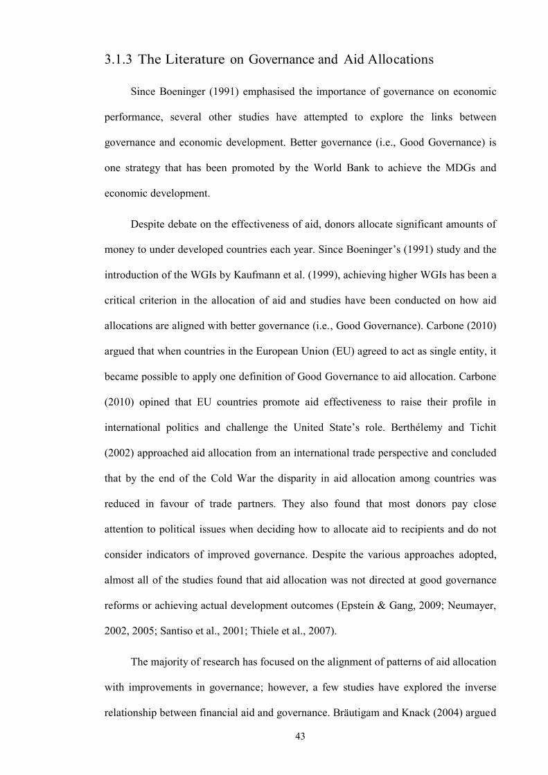
3.1.3 The Literature on Governance and Aid Allocations
Since Boeninger (1991) emphasised the importance of governance on economic
performance, several other studies have attempted to explore the links between
governance and economic development. Better governance (i.e., Good Governance) is
one strategy that has been promoted by the World Bank to achieve the MDGs and
economic development.
Despite debate on the effectiveness of aid, donors allocate significant amounts of
money to under developed countries each year. Since Boeninger’s (1991) study and the
introduction of the WGIs by Kaufmann et al. (1999), achieving higher WGIs has been a
critical criterion in the allocation of aid and studies have been conducted on how aid
allocations are aligned with better governance (i.e., Good Governance). Carbone (2010)
argued that when countries in the European Union (EU) agreed to act as single entity, it
became possible to apply one definition of Good Governance to aid allocation. Carbone
(2010) opined that EU countries promote aid effectiveness to raise their profile in
international politics and challenge the United State’s role. Berthélemy and Tichit
(2002) approached aid allocation from an international trade perspective and concluded
that by the end of the Cold War the disparity in aid allocation among countries was
reduced in favour of trade partners. They also found that most donors pay close
attention to political issues when deciding how to allocate aid to recipients and do not
consider indicators of improved governance. Despite the various approaches adopted,
almost all of the studies found that aid allocation was not directed at good governance
reforms or achieving actual development outcomes (Epstein & Gang, 2009; Neumayer,
2002, 2005; Santiso et al., 2001; Thiele et al., 2007).
The majority of research has focused on the alignment of patterns of aid allocation
with improvements in governance; however, a few studies have explored the inverse
relationship between financial aid and governance. Bräutigam and Knack (2004) argued
44
that while financial aid can remove budget constraints for governments and enable them
to invest in their legal systems and strengthen their domestic institutions, financial aid
often creates obstacles that hinders the development of good governance. Further,
Bräutigam and Knack (2004) found that there was a robust statistical relationship
between high levels of aid and the deterioration of governance in Africa.
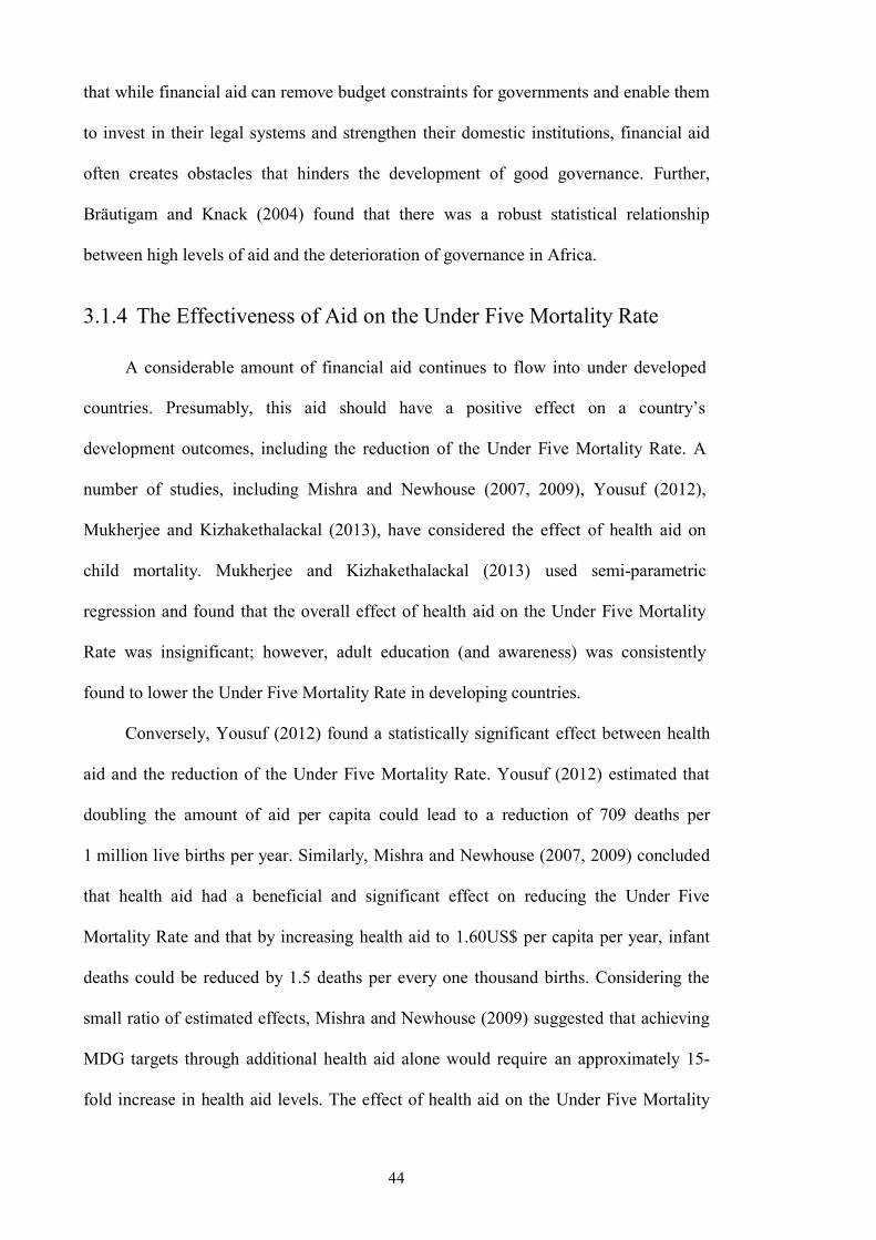
3.1.4 The Effectiveness of Aid on the Under Five Mortality Rate
A considerable amount of financial aid continues to flow into under developed
countries. Presumably, this aid should have a positive effect on a country’s
development outcomes, including the reduction of the Under Five Mortality Rate. A
number of studies, including Mishra and Newhouse (2007, 2009), Yousuf (2012),
Mukherjee and Kizhakethalackal (2013), have considered the effect of health aid on
child mortality. Mukherjee and Kizhakethalackal (2013) used semi-parametric
regression and found that the overall effect of health aid on the Under Five Mortality
Rate was insignificant; however, adult education (and awareness) was consistently
found to lower the Under Five Mortality Rate in developing countries.
Conversely, Yousuf (2012) found a statistically significant effect between health
aid and the reduction of the Under Five Mortality Rate. Yousuf (2012) estimated that
doubling the amount of aid per capita could lead to a reduction of 709 deaths per
1 million live births per year. Similarly, Mishra and Newhouse (2007, 2009) concluded
that health aid had a beneficial and significant effect on reducing the Under Five
Mortality Rate and that by increasing health aid to 1.60US$ per capita per year, infant
deaths could be reduced by 1.5 deaths per every one thousand births. Considering the
small ratio of estimated effects, Mishra and Newhouse (2009) suggested that achieving
MDG targets through additional health aid alone would require an approximately 15-
fold increase in health aid levels. The effect of health aid on the Under Five Mortality
45
Rate is still under debate. Notably, the effectiveness of health aid in reducing the Under
Five Mortality Rate appears to differ under various model specifications.
3.1.5 Contributions of this Study
Numerous studies in this area suggest that socioeconomic status has a significant
effect on the Under Five Mortality Rate. One of the most important socioeconomic
institutions in any country is its level of governance. In much of the literature,
governance has been studied as criteria for health aid allocation. However, only a few
studies (e.g., Lin et al. 2014) have examined governance as an independent effective
factor on the Under Five Mortality Rate. Lin et al. (2014) found that good governance
(along with other social determinants) has a positive effect in reducing the Under Five
Mortality Rate. In addition to domestic factors (e.g., governance) foreign factors (e.g.,
financial aid) have also been linked to the Under Five Mortality Rate. Regardless of the
motivation of financial aid, the effect of this aid on economic development (and
specifically, on health outcomes) remains questionable.
This study sought to determine the effect of governance and health aid (i.e., the
financial aid allocated to the health sector) on child mortality. Thus, similar to the
studies of Mishra and Newhouse (2007, 2009) and Lin et al. (2014), this study can be
categorised as macro level research. In this study, two branches of the relevant
literature are combined17. Specifically, this study sought to examine whether health aid
and governance can reduce the Under Five Mortality Rate.
The next section begins by introducing a model and explaining how each of the
variables of choice can affect the Under Five Mortality Rate. Next, the methodology
chosen to address this research question is explained. Following this, a snapshot of the
17 That is, both the effect of governance on the Under Five Mortality Rate (see Lin et al. 2014) and the effect of health aid on the Under Five Mortality Rate (see Mishra & Newhouse 2007, 2009; Mukherjee & Kizhakethalackal 2013; Yousuf 2012) are investigated.
46
dataset is presented and an explanation is given on how each of the variables was
measured. Finally, the results of the regression are reviewed and the robustness of the
results checked using a different methodology.
3.2 The Model
In this study, the Under Five Mortality Ratio (i.e., the probability per 1,000 live
births that a newborn baby will die before reaching the five years of age) was the main
dependent variable used to examine the role of governance and health aid on child
mortality. The two main independent variables were the level of governance and the
amount of health aid per capita. To explore the true impact of governance and health
aid on the Under Five Mortality Rate, the other characteristics of countries (e.g.,
education and population) had to be controlled.
The Under Five Mortality Rate is a household level indicator and has been
typically studied at the micro level. However, it is also an important indicator of a
country’s level of development. Thus, it has also been studied from a macro level and a
Mukherjee & Kizhakethalackal, 2013). Possible macroeconomic factors that could
affect the Under Five Mortality Rate include the status of a country’s health sector,
governments’ budget allocations and foreign development aid allocations. In most
cases, it is impossible to study these effects at a micro level; however, while the effect
of a government’s expenditure in the health sector cannot be studied at a
microeconomic level, available data can be used to examine the linkage in macro level
analysis. Examining the impact of macroeconomic indicators on the Under Five
Mortality Rate is possible, as child mortality rates, derived from household surveys, are
nationally representative. Additionally, the Under Five Mortality Rate represents a
probability and is a ratio that can be applied to macro analyses.
47
Thus, this study considered the role of governance and health aid allocation on
the Under Five Mortality Rate at a macro level using macroeconomic indicators. Where
the indicators and measures were derived from household surveys, all the indicators
were nationally representative. To provide a clearer outline of the model and explain
how countries’ different characteristics affect the Under Five Mortality Rate, each
variable of choice related to the Under Five Mortality Rate is discussed. Additionally,
consideration is given to how these variables can change the effectiveness of
governance and health aid on the Under Five Mortality Rate.
3.2.1 Links between Health Aid and the Under Five Mortality Rate
The effectiveness of health aid on the Under Five Mortality Rate has been the
subject of debate within the literature. Some studies (e.g., Mishra & Newhouse, 2007,
2009; Yousu, 2012) have focused on the positive influence of health aid, arguing that it
can remove budget constraints and help countries to improve the wellbeing of adults
and children. However, others studies (e.g., Mukherjee & Kizhakethalackal, 2013) have
found no statistically significant link between health aid and the Under Five Mortality
Rate and have argued that health aid has no effect on health outcomes such as the
Under Five Mortality Rate.
Health aid is defined as any form of financial aid allocated to the health sector.
Researchers examining the effect of health aid on health outcomes have struggled with
the fact that it can be difficult to determine whether the aid allocated has been used for a
specific purpose. This study had to contend with this very issue, as it was unclear
whether health aid funds had been allocated to programmes directed at reducing the
Under Five Mortality Rate. However, health aid funds allocated to different health
programmes could also indirectly affect the Under Five Mortality Rate; for example,
using health aid funds to equip medical centres, employ trained staff and improve the
quality of nutrition could help to fight the causes associated with the Under Five
48
Mortality Rate. Further, given that the Under Five Mortality Rate is a targeted MDG, it
is logical to assume that recipient countries are using a portion of their health aid funds
to reduce the Under Five Mortality Rate.
This study evaluates the effectiveness of aid allocated to the health sector in the
same year. Additionally, the effectiveness of last year’s allocated health aid is
examined. The hypotheses of this chapter are similar to those of Mishra and Newhouse
(2007).
3.2.2 Can Governance affect the Under Five Mortality Rate?
The other important explanatory variable in this study’s model is the level of
governance. Governance has frequently been studied as a factor in health aid allocation;
however, its influence on child mortality and health aid has not been fully explored.
Theoretically, an increase in good governance could affect the Under Five Mortality
Rate. First, it could change the effectiveness of foreign health aid (e.g., Good
Governance could lead to health aid being allocated to the people most in need).
Second, better governance could affect a country’s local and domestic health
expenditure. Additionally, in well-governed countries, people can vote for policies
directed at improving health and wellbeing, including polices aimed at lowering the
Under Five Mortality Rate. Further, in countries with higher levels of governance,
existing health budgets can be altered to work more effectively and efficiently.
3.2.3 Health Related Indicators and the Under Five Mortality Rate
The Under Five Mortality Rate is one of several highly interrelated health
development issues (others include Human Immunodeficiency Virus (HIV), Acquired
Immune Deficiency Syndrome (AIDS) and vaccinations). Black et al. (2010) found that
almost 68 per cent of child mortality is caused by infectious disease. Thus, vaccinations
against common childhood diseases could have a significant role in reducing the Under
49
Five Mortality Rate. In this model, the rates of immunisation against Diphtheria,
Pertussis and Tetanus (DPT) were used to control for the effects of infectious disease.
The other variable controlled for was the levels of HIV and AIDS in countries. Official
figures for this indicator refer to the percentage of the population (aged between 15–49-
years-old) infected with HIV/AIDS. HIV/AIDS is one of the most serious health issues
in under developed countries, as if an individual with HIV/AIDS becomes ill with
another (even a minor) infection, it could be fatal. Thus, in this model a control for HIV
prevalence was also included.
Compared to developed countries, in under developed and (many) developing
countries, a significant proportion of women give birth attended by un-trained people or
without any assistance. The Under Five Mortality Rate refers to child mortality, not
neonatal mortality; however, studies show that health care is important before, during
and after pregnancy, as trained staff can educate mothers on the nutritional needs of
their children and the possible risks that they may encounter. To control for the
possibility that the number of trained staff present at births affect the Under Five
Mortality Rate, the percentage of births attended by trained staff members was also
included as a control variable.
Amouzou and Hill (2004), Amouzou et al. (2012) and Mishra and Newhouse
(2007) specified access to sanitation facilities as another health related indicator that
should be controlled. Poor sanitation and a lack of adequate sewage systems have been
found to be the main method of transmission of infections and diseases. Additionally,
the proportion of funds that governments allocate to the health sector is another factor
that might affect the Under Five Mortality Rate as a health outcome. Thus, in this study,
the total health expenditure of a country (as a percentage of the GDP) was used to
control for the level of government health expenditure.
50
A number of studies (e.g., Amouzou & Hill, 2004, Amouzou et al., 2012, Bhutta
et al., 2010, Lozano et al., 2011, Mishra & Newhouse, 2007, 2009, Rajaratnam et al.,
2010, UNICEF, 2011 and Yousuf, 2012) have found that existing levels of health
related factors (e.g., the share of health expenditure of the GDP, births attended by
trained staff, immunisation rates, the prevalence of HIV/AIDS and access to sanitation
facilities) can affect the Under Five Mortality Rate.
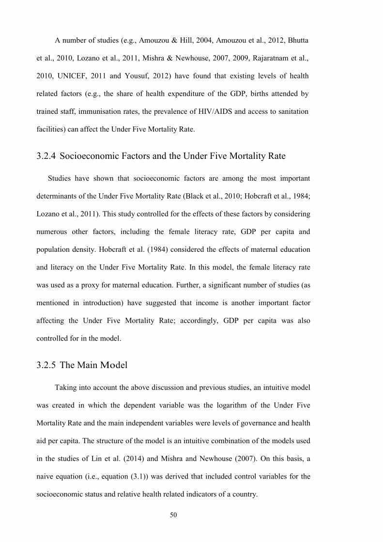
3.2.4 Socioeconomic Factors and the Under Five Mortality Rate
Studies have shown that socioeconomic factors are among the most important
determinants of the Under Five Mortality Rate (Black et al., 2010; Hobcraft et al., 1984;
Lozano et al., 2011). This study controlled for the effects of these factors by considering
numerous other factors, including the female literacy rate, GDP per capita and
population density. Hobcraft et al. (1984) considered the effects of maternal education
and literacy on the Under Five Mortality Rate. In this model, the female literacy rate
was used as a proxy for maternal education. Further, a significant number of studies (as
mentioned in introduction) have suggested that income is another important factor
affecting the Under Five Mortality Rate; accordingly, GDP per capita was also
controlled for in the model.
3.2.5 The Main Model
Taking into account the above discussion and previous studies, an intuitive model
was created in which the dependent variable was the logarithm of the Under Five
Mortality Rate and the main independent variables were levels of governance and health
aid per capita. The structure of the model is an intuitive combination of the models used
in the studies of Lin et al. (2014) and Mishra and Newhouse (2007). On this basis, a
naive equation (i.e., equation (3.1)) was derived that included control variables for the
socioeconomic status and relative health related indicators of a country.
51
(3.1)
In equation (3.1), U5MR refers to the mortality rate of children under five-years-
old per 1,000 live births; GG is the proxy for governance18 and H.AidPC shows the
health sectors allocated international development aid flow per capita. In addition to the
main variables, control variables were also included to control for potentially effective
health characteristics and health measures. This group of control variables is referred to
as XH and included: (a) immunisation against DPT (as a percentage of children aged
between 12–23 months old); (b) health expenditure totals (as a percentage of the GDP);
(c) births attended by trained health staff (as a percentage of the total births); (d) the
prevalence of HIV (as a percentage of the population aged between 15-–49 years of
age); and (e) improved sanitation facilities (as a percentage of the population with
access to sanitation facilities).
Variables were also included as a vector of socioeconomic control. These
variables were noted as XSE and included: (a) a logarithm for GDP per capita (i.e., PPP
current international $); (b) an adult total for the female literacy rate (as a percentage of
females aged 15 years and older); and (c) an error term (𝜖𝑖𝑡).
In this model, the coefficients of and are points of interest. According to
the literature (see Lin et al., 2014), a negative 𝛽2 implies a higher level of governance, a
factor that could reduce child mortality. Additionally, was expected to be negative,
as studies (e.g., Kosack, 2003) have found that better governance can help the flow of
aid and increase the quality of life of individuals in recipient countries.
18 This was constructed using PCA (see Appendix 6.4).
52
3.3 Data
In this study, the Under Five Mortality Rate (i.e., the dependent variable) was the
probability of dying between birth and exactly five years of age (expressed per 1,000
live births). Birth and death data, derived from civil registration documents, censuses
and/or household surveys (i.e., WHO, 1994), was used to construct nationally
representative values. The Under Five Mortality Rate data is available through the
World Development Indicator of the World Bank database. The Under Five Mortality
Rate has a mean of 47.93 that varies from 2.2 to 266.4 and, as a trend, has been steadily
decreasing since 1995 (see Figure 3.1).
Source: The World Bank, World Development Indicators Figure 3.1: Trend of the Average Under Five Mortality Rate
The indicator for the level of governance is one of the main explanatory variables
in this study. Governance (and its various dimensions) has been in several studies;
however, there is no known indicator for the concept of the level of governance as a
whole. Thus, a proxy indicator for the level of governance was constructed using a PCA
on Kaufmann et al.’s (1999) WGIs.19
19 In Appendix 6.4, the methodology is explained; specifically, it is shown how the methodology was used to create a proxy for governance.
53
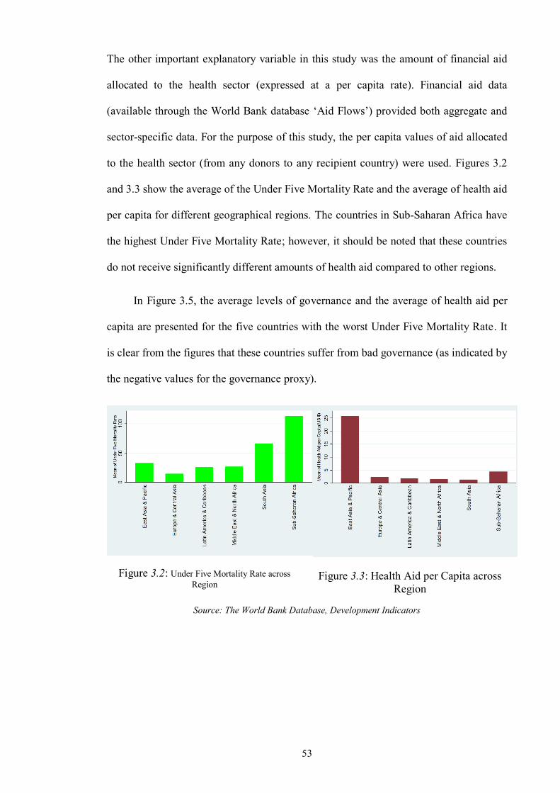
The other important explanatory variable in this study was the amount of financial aid
allocated to the health sector (expressed at a per capita rate). Financial aid data
(available through the World Bank database ‘Aid Flows’) provided both aggregate and
sector-specific data. For the purpose of this study, the per capita values of aid allocated
to the health sector (from any donors to any recipient country) were used. Figures 3.2
and 3.3 show the average of the Under Five Mortality Rate and the average of health aid
per capita for different geographical regions. The countries in Sub-Saharan Africa have
the highest Under Five Mortality Rate; however, it should be noted that these countries
do not receive significantly different amounts of health aid compared to other regions.
In Figure 3.5, the average levels of governance and the average of health aid per
capita are presented for the five countries with the worst Under Five Mortality Rate. It
is clear from the figures that these countries suffer from bad governance (as indicated by
the negative values for the governance proxy).
Figure 3.2: Under Five Mortality Rate across Region
Figure 3.3: Health Aid per Capita across Region
Source: The World Bank Database, Development Indicators
54
Figure 3.3: Governance in worst Five Countries in Under Five Mortality Rate
Figure 3.4: Health Aid Per Capita in worst Five Countries in Under Five Mortality
Rate
Source: The World Bank Database, Development Indicators
Previously, it was suggested that a socioeconomic factor that might affect the
Under Five Mortality Rate was maternal education. In this study, an adult female
literacy rate was used as a proxy for maternal education. However, an issue in relation
to the use of this variable arose, as there was a lack of sufficient data with desirable
frequency. To overcome this problem it was assumed that the literacy rate would not
change rapidly and that it would have a monotonous trend over time. Further, it was
assumed that the literacy rate could be held constant for the years where no data was
available.
3.3.1 The Variables and their Definitions
Table 3.1 presents the official definitions of the variables and their data sources. It
should be noted that while most of the variables were exported from the World Bank
database of World Development Indicators, the proxy for governance indicator was
constructed using the PCA.
55
Table 3.1: Definitions of the Variables and their Data Source
Variable Definition Source of Data
The Worldwide Governance Indicators (WGIs)
These aggregate indicators combine the views of a large number of enterprises, citizens and expert survey respondents in industrial and developing countries. It includes aggregate and individual governance indicators for 215 countries and territories for the period of 1996−2012 for six dimensions of governance
Worldwide Governance Indicators database
Health Aid (Development Aid allocated to health sectors)
Development Aid refers to the financial aid given by governments and other agencies to support the economic, environmental, social and political development of developing countries. It can be distinguished from humanitarian aid because of its focus on alleviating poverty in the long term (i.e., it does not refer to aid given as a short term response)
The World Bank database of ‘Aid Flows’
Under Five Mortality Rate (per 1,000 live births)
The Under Five Mortality Rate is the probability per 1,000 live births that a newborn baby will die before reaching the age of five, if subject to current age-specific mortality rates
The World Development Indicators
Literacy Rate, adult female (percentage of females aged 15 years and above)
The literacy rate (in a percentage form) of female adults (aged 15 years and above) who can, with understanding, read and write a short, simple statement on their everyday life
The World Development Indicators
GDP per capita (current US$)
GDP per capita is gross domestic product divided by the mid year population. Data is in current US dollars
The World Development Indicators
Immunisation, DPT (percentage of children aged 12–23 months)
Child immunisation measures the percentage of children aged between 12–23 months who received vaccinations before 12 months of age or at any time before the survey
The World Development Indicators
Prevalence of HIV, total (percentage of the population aged between 15–49)
The prevalence of HIV refers to the percentage of people aged 15–49 who are infected with HIV
The World Development Indicators
Births attended by trained health staff (percentage of total)
Births attended by trained health staff refers to the percentage of deliveries attended by staff trained to give the necessary supervision, care and advice to women during pregnancy
The World Development Indicators
Improved sanitation facilities (percentage of population with access)
Access to improved sanitation facilities refers to the percentage of the population using improved sanitation facilities. The improved sanitation facilities include flush/pour systems (to piped sewer systems, septic tanks and pit latrines), ventilated improved pits (VIP) latrines, pit latrines with slabs and composting toilets
The World Development Indicators
Health expenditure, total (percentage of GDP)
The total health expenditure is the sum of public and private health expenditure. It covers the provision of health services (preventive and curative), family planning activities, nutrition activities and emergency aid designated for health, but does not include provision of water and sanitation
The Bank Development Indicators
3.3.2 Descriptive Statistics
Table 3.2 presents a summary of statistics for the variables used in the sample.
The sample size of this study comprised 534 observations covering 78 countries,
56
including 73 low and mid-level income countries of which almost 60 were located in
Latin America and Sub-Saharan Africa. The mean of the Under Five Mortality Rate in
the sample was approximately 83 deaths per 1,000 live births (see Table 3.2). Further,
in the sample the constructed proxy for good governance varied from a maximum of
3.159 (with Chile having the best rate in 2002) to a minimum of -3.823 (with Haiti
having the worst rate in 2004).
In addition to the main variables, the control variables were included in the
dataset. The maximum scores for some of these variables were as expected; however,
the minimums revealed shocking results. Specifically, the immunisation rate against
DPT had a statistical minimum of 19. Thus, a significant number of countries require
immunisation programmes. Additionally, the percentage of the population with ‘Access
to Improved Sanitation’ was approximately 7.5 per cent, a shockingly low figure. As
stated above, health expenditure as a proportion of the annual GDP was thought to be a
factor that could affect the Under Five Mortality Rate. The dataset showed that across
the sample this variable varied from 1.612 per cent (the minimum in Equatorial Guinea)
to approximately 17 per cent (the maximum in Sierra Leone).
57
Table 3.2: Summary Statistics
Variable Obs. Mean Std. Dev. Min Max
Mortality rate, Children Aged Under 5 (deaths per 1,000 live births)
534 82.081 48.410 6.3 219.4
Proxy Indicator for Good Governance 534 -1.061 1.356 -3.823 3.159
Health Aid Per Capita 534 3.653 4.208 0.002 33.31
Log of GDP Per Capita 534 6.959 1.117 4.682 9.645
Literacy Rate, Female Adults (percentage of females aged 15 and above)
534 61.241 26.059 8.057 99.79
Health Expenditure Total (percentage of GDP) 534 6.302 2.34 1.612 16.900
Immunisation, DPT (percentage of children aged 12–23 months)
534 80.88 16.16 19 99
HIV Prevalence 534 4.172 6.384 0.100 26.900
Access to Improved Sanitation 534 44.944 28.749 7.500 97.300
Births by Trained Staff 155 69.972 25.388 5.700 99.900
3.4 Methodology
As stated in previous sections, the dataset consists of both time series and cross
sections. Thus, the main equation was constructed and estimated in panel data format.
LS panel data is possibly the simplest econometric methodology for estimating the out
of interest parameters in panel data format. This data provided insight into the general
links between the main variables of this study; however, some methodological issues
had to be addressed.
In normal panel data analysis, it is assumed that the error term is homoscedastic
and is not correlated to any of the explanatory variables. However, in a practical sense,
58
in models with a significant number of cross sections and time series, the error term can
be correlated within cross section and with times. Thus, to control for these correlations
(known as time effects and fixed effects) researchers use panel data with fixed effects.
Additionally, there could be a correlation between error terms across different times
(this occurs in most time series analyses). However, according to Baltagi (2013), when
the number of time periods is relatively small, as compared to the number of cross
sections, robust standard errors can solve the autocorrelation problem. Thus, to
overcome the heteroscedasticity and autocorrelation problems, the clustering option
available in Stata® was used (as suggested by Wooldridge, 2010).
3.4.1 Methodological Concerns
A fixed effects method would have addressed the heterogeneity that occurs in
normal Ordinary Least Squares (OLS) by controlling for country-specific individual
effects; however, it could have also yielded a biased result for the model. Biases may
occur for a number of reasons, including the correlations between lagged health aid
variables and error terms20 (Mishra & Newhouse, 2009). A consideration of the health-
specific control variables could have been beneficial in estimating the equation;
however, these variables could also have caused an endogeneity problem, as an
unknown factor could have affected both the Under Five Mortality Rate (i.e., the
dependant variable) and any of the other health-specific control variables (e.g., the
prevalence of HIV).
3.4.2 Generalised Method of Moments Dynamic Panel
Adopting the approach of Mishra and Newhouse (2009), the Generalised Method
of Moments (GMM) Dynamic Panel Data were used to account for the potential
20 Thus, the unobserved effect (as captured by ) might carry information from the previous year’s health aid.
59
endogeneity issues that might be caused by variables of less interest to this study. The
GMM was introduced by Arellano and Bond (1991) and further developed by Blundell
and Bond (2000) and Bond (2002). Under the GMM, rather than the traditional
application of instrumental variables, variables are lagged and used as instruments for
their level or differences. In the GMM, there are two main equations (see the equations
in (3.2)); the first is a level equation and the second, a differenced equation.
(3.2)
Lagged differences of variables (e.g., 𝐻.𝐴𝑖𝑑 − 𝐻.𝐴𝑖 ) are used as
instruments in the level equation and lagged variables (i.e., ) are used as
instruments in the difference equation. The GMM panel data is used instead of the
difference GMM for three main reasons. First, in the GMM, fixed effects are washed
out in the equation after the difference is obtained. Second, the GMM provides results
that are more plausible when the main variable is persistent (Blundell & Bond, 2000).21
Third, the GMM yields better results for panels with a small T (time), but a relatively
large number N (Blundell & Bond, 2000), as was the case in this study.
Additionally, as mentioned above, the main focus of this study was to explore the
effect of both governance and health aid upon the Under Five Mortality Rate. In
equations (3.2), the level variable of health aid was considered and, in some
specifications of the results section, one lagged period of this variable was included.
21 ‘When the series are near unit root process, the instruments used in the first-differenced equation become weak and thus System GMM would have better results’—Blundell and Bond, 2000. The Fisher-type unit root test was applied on the Under Five Mortality Rate and the results suggested a unit root process for the Under Five Mortality Rate.
60
An important step in applying the GMM is to identify the endogenous, exogenous
and predetermined variables. Strictly exogenous variables refer to variables that do not
correlate with the error term (i.e. ). Thus, if it is assumed that a variable such as W is
strictly exogenous, the definition implies for s and t. Strictly
exogenous variables enter in to the instrument matrix independently. In this model, it
was assumed that governance was strictly exogenous, as it would have been impossible
for any shock in the Under Five Mortality Rate to change the level of governance.
Another exogenous variable that was considered was population density. Similar to
governance, any shock on the Under Five Mortality Rate would not have changed the
levels of urbanisation or population density. Additionally, as suggested by Roodman
(2009a) the time effects (i.e., the year dummies) were considered as another strictly
exogenous variable.22
The next step in the application of the GMM was the identification of
predetermined variables. Predetermined variables are variables correlated with lagged
error terms. If W is taken as an example of a predetermined variable, the assumption
yields and . Predetermined
variables might also be endogenous and may enter the instrument matrix with a
minimum of two lags. Conversely, other predetermined variables, without endogeneity,
enter the matrix with at least one lag. In the model, it was also assumed that the health
sector-specific control variables were both predetermined and endogenous. They were
considered to be predetermined variables, as any shock on the Under Five Mortality
Rate would have changed the number of physicians or the share of GDP’s health budget
in the next period (i.e., in the next year). Thus, health sector-specific variables were
22 ‘The autocorrelation test and the robust estimates of the coefficient standard errors assume no correlation across individuals in the idiosyncratic disturbances. Year dummies make this assumption more likely to hold’—Roodman, 2009.
61
considered to be predetermined and endogenous and entered into the instrument matrix
with at least two lags.
To estimate the main equation with the above specifications, the Stata package
implemented by Roodman (2009a) was utilised. One of the significant advantages of
Roodman’s (2009a) package is that it reports all Sargan/Hansen J statistics and results
in autocorrelation tests. It should be noted that it is possible that this model suffers from
autocorrelation and heteroscedasticity. Accordingly, to control for autocorrelation and
heteroscedasticity, the cluster and robust option in the Roodman (2009a) package was
used to create HAC23 corrected standard errors in the estimation. Additionally, a two-
step GMM procedure (also available by Roodman, 2009a) was used that included
Windmeijer’s (2005) correction for finite sample bias.
3.5 Results
3.5.1 Results of the Dynamic Panel Data
GMM Dynamic Panel data was used to estimate the parameters. The results are
displayed in Table 3.3. In columns (1) to (6) one lagged period of health aid is
considered; in columns (7) to (12) the value level of health aid (i.e., health aid without
any lag) was used along with the control variables. As suggested by Roodman (2009a),
and similar to the approach taken by Mishra and Newhouse (2009), in the regression
results, the number of instruments used in the process of estimating the GMM was
reported with other relevant criterion.
According to the results, governance has negative significant effect on the Under
Five Mortality Rate across almost all specifications. These results aligned with the
existing literature (e.g., the study of Lin et al., 2014). Further, the coefficients of health 23 The heteroscedasticity and autocorrelation.
62
aid per capita in all specifications (see columns (7) to (12)) were not statistically
significant nor were the coefficients of the last year’s health aid per capita24. Columns
(6) and (12) show the interactive terms between governance and health aid per capita (or
lagged health aid per capita). As shown in the table, the relative coefficients were not
significant.
As mentioned above, in the GMM Dynamic Panel, lagged variables were used as
instruments to estimate a system of equations. Thus, the numbers of instruments
reported in the table actually represent the number of lagged variables used for the
purpose of estimation. The number of instruments and the number of lagged variables
are highly dependent on the width of the panel (i.e., the number of years included in
regression). As stated by Roodman (2009b), a large number of instruments can be a
practical issue, as, if the number of instruments becomes relatively too large, the
regression may suffer from over identification and loss of degrees of freedom. Further,
as Roodman (2009a) also mentioned, the GMM Dynamic Panels are efficient in datasets
with a relatively small T and large N.
It was assumed that the regression in this study did not suffer from an over
identification problem or a large number of instruments. There are at least three reasons
to support this assumption. First, the data used in the regressions covered approximately
80 countries over a maximum period of 11 years.25 Thus, the N was relatively large in
the data. Second, Roodman’s (2009b) strategy was adopted, whereby the problems
related to having a large number of instruments was avoided by controlling the
maximum number of lags in the variables used as instruments. In the results (see Table
3.3), a maximum three-year lag was considered. Third, as a consequence of there being
a relatively large number of countries in the data, there was a sufficient degree of
24 The effect of births attended by trained staff was also tested; however, the coefficient was insignificant in all specifications and thus the results were not reported. 25 For a detailed list of the countries used in the sample, see Appendix 6.5.
63
freedom in the regressions. Conversely, as pointed out by Bazzi and Clemens (2013), in
the GMM weak instruments could also cause significant differences in the estimation
results in a macroeconomic analysis. The issue of weak instruments in other types of
estimators and, specifically, in estimators using the GMM, has been the subject of
various studies, tests and software packages (e.g., the Weakiv package by Finlay and
Magnusson, 2009). In this study, the Weakiv package was used to show that the model
did not suffer from weak instruments (see Table 3.3 for the relative test results). The
results suggest that the model and specifications did not suffer from any weak
instrument issues. Further, the stability of regressions in GMM Dynamic Panels is
commonly suggested by two criteria: the Sargan test26 and Arellano and Bond (1991)’s
(0.00371) (0.00304) (0.00381) (0.0142) (0.00286) (0.00454) (0.00376) (0.00457) (0.0113) Log of Population Density
-0.00400 -0.0392 -0.0266 -0.0276 -0.0435 -0.0446 (0.0286) (0.0311) (0.0335) (0.0314) (0.0402) (0.0357) (Lagged) Health Aid per capita × Good Governance
0.000392 0.000559
(0.000425) (0.000337) Constant Yes Yes Yes Yes Yes Yes Yes Yes Yes Yes Yes Yes Regional Dummies No No Yes No Yes Yes No No Yes No Yes Yes Hansen Test: P-value 0.998 0.999 0.999 0.998 0.998 0.98 0.997 0.998 0.998 0.999 0.999 0.99 AR(2) Test: P-value 0.702 0.402 0.105 0.273 0.104 0.186 0.407 0.811 0.147 0.78 0.203 0.17 Moreira 2003; Kleibergen 2007–Test: P-value 0.998 0.999 0.999 0.999 0.999 0.999 0.998 0.999 0.999 0.999 0.999 0.999 J Over Identification Test – Test: P-value 0.998 0.999 0.999 0.999 0.999 0.998 0.998 0.999 0.999 0.998 0.998 0.998 Anderson and Rubin (1949)—AR Test: P-value 0.997 0.998 0.999 0.999 0.999 0.999 0.997 0.999 0.999 0.9997 0.999 0.999 Number of Instruments 210 243 248 244 249 277 219 252 257 253 253 286 Observations 548 534 534 534 534 534 559 544 544 544 544 544 Number of Countries 80 80 80 80 80 80 78 78 78 78 78 78 The dependant variable was the logarithm of the Under Five Mortality Rate and the robust HAC corrected standard errors in parentheses. *** p<0.01, ** p<0.05, * p<0.1. A robust two-step GMM was used that included Windmeijer’s (2005) correction for finite samples. Time fixed effects were considered in all regressions. A detailed list of countries is provided in Appendix 6.5.
65
As robust standard errors were reported, the Hansen test was performed rather
than the Sargan test. The null hypothesis of both tests is that ‘the instruments as a group
are exogenous’; however, a Hansen test is reported when a robust option is used. In
relation to both the Hansen and Sargan tests, higher P-values are appreciated. Further,
the Arellano and Bond (1991) autocorrelation test evaluates the hypothesis of ‘No
autocorrelation with X lag(s)’ and was applied to the differenced residuals. Thus, in
Table 3.3 the P-value for the null hypothesis of ‘No Autocorrelation with two lags (or
am AR (2) process)’ was reported. Based on the reported statistics, all of the
specifications in Table 3.3 appear to be acceptable. As shown in Figure 3.3, health aid
and the Under Five Mortality Rate vary across different regions. To control for these
variations, regional dummies were included in the regressions. Regional dummies were
also used where there were any geographical characteristics common across countries
that could have affected the Under Five Mortality Rate of all the countries in a specific
region.
The insignificant coefficients of health aid per capita and lagged health aid per
capita aligned with previous research (e.g., Mukherjee & Kizhakethalackal, 2013).
Additionally, the significant negative coefficient of the logarithm of GDP per capita was
as expected and as found in previous studies. The negative effect of adult female
literacy and the positive effect of HIV prevalence on the Under Five Mortality Rate
were statistically significant across all specifications. Despite the results of other
studies, in this study, no statistical evidence was found of health expenditure (as a
proportion of the GDP) having an effect on the Under Five Mortality Rate. Similarly,
there was no evidence suggesting that population density had an effect on the Under
Five Mortality Rate and no consistent significant effect was found in relation to the rate
of access to improved sanitation.
66
Overall, the results do not confirm the hypothesis that health aid (either in the
level or lagged form) affected the Under Five Mortality Rate. However, the results do
show that the role of governance has a statistically significant and negative effect on the
Under Five Mortality Rate. According to estimations in this study, a one unit increase in
the level of governance could decrease the Under Five Mortality Rate by approximately
0.1 per cent.
3.5.2 Robustness Check: Quantile Regression
The results presented in the previous section revealed that governance has a
statistical significant negative impact on the Under Five Mortality Rate. The findings in
relation to the insignificant role of health aid aligned with previous studies (e.g.,
Mukherjee & Kizhakethalackal, 2013); however, to check the robustness of the results
for both governance and health aid, a cross section quantile regression was conducted.
As a robustness check, quantile regression was deemed suitable for two main
reasons. First quantile regression would reveal whether the results and findings were
consistent across all levels of the Under Five Mortality Rate. In the dataset, some
countries had extreme Under Five Mortality Rates (e.g., Somalia had a rate of 400)
whereas other situations were less severe and had lower values (e.g., Turkmenistan had
a rate of 80). The quantile regression provided insight into the stability of the results.
Second, quantile regression was used because previous studies (e.g., Mukherjee &
Kizhakethalackal, 2013) have shown that the effect of health aid on the Under Five
Mortality Rate could be different in semi-parametric estimations. Thus, there was a
need to test the equivalent hypothesis for both governance and health aid using quantile
regression as one of the non-parametric regression methods.27
27 Quantile regressions can be categorised as non-parametric models, as they relax any preliminary assumptions about the parametric distribution of the errors.
67
To run the quantile regression, the dataset was collapsed using the means of
variables across time. Collapsing the dataset also allowed the stability of the results in
the cross section models to be checked alongside the panel data. Thus, the main
equation changed to:
(3.3)
Where could be 0.25, 0.50 or 0.75 quantiles. The results of the quantile
estimation are presented in Table 3.4. In columns (1) to (3), the results of the different
specifications for the three quantiles were presented. The specifications varied across
the columns; however, the overall results appeared to be consistent across almost all
specifications and quantiles (i.e., the four statistically significant determinants of the
Under Five Mortality Rate (HIV prevalence, female literacy and immunisation rates as
measured against DPT and the Log of GDP per capita) were robust across models. No
evidence was found of health expenditure in the GDP having any effect on the Under
Five Mortality Rate. Similarly, the results showed that access to improved sanitation did
not have any statistically significant effect on the Under Five Mortality Rate.
The dependent variable is the logged Under Five Mortality Rate. All the variables were averaged over time. *** p<0.01, ** p<0.05, * p<0.1. Bootstrap standard errors are in parentheses. Seven geographical regions’ dummies were included in the regressions.
69
Based on the results set out in Table 3.4, there was no evidence of health aid
having any effect on the Under Five Mortality Rate. Conversely, in relation to
governance a negative effect was found in the quantile regression. Importantly, the
magnitude of the effect of governance on the Under Five Mortality Rate (see Table 3.4)
is quite similar to that detailed in Table 3.3. These robust findings across different
models suggest that governance has a solid negative effect on the Under Five Mortality
Rate.
3.6 Chapter Conclusion
According to findings of this study, governance has negative significant effect on
the Under Five Mortality Rate; however, there was no statistical evidence that health aid
per capita had an effect on the Under Five Mortality Rate. Health aid per capita was
insignificant in both parametric and semi-parametric models. However, the following
three determinants were also found to have a robust effect on the Under Five Mortality
Rate: adult female literacy rate, prevalence of HIV and immunisation against DPT.
The conclusions drawn in relation to the affect of health aid per capita align with
the studies of Mukherjee and Kizhakethalackal (2013). However, a solid, consistent
conclusion can be derived in relation to the effect of governance on the Under Five
Mortality Rate; that is, there is a statistically significant negative effect. This conclusion
was robust across parametric and non-parametric settings and it was also replicated in
panel data analysis and quantile regression across cross sections. Conclusions on the
magnitude of the effect of governance can also be drawn; a one unit change in
governance appears to reduce the Under Five Mortality Rate by approximately 0.1 per
cent.
70
Reducing child mortality rates is not only one of the targets of the MDGs, but is also
an important target for all developing countries. As the eighth MDG, both developed
countries and development organisations provide financial aid to under developed and
less developed countries. The results of this study show the effectiveness of health aid
in reducing the Under Five Mortality Rate is not conclusive. Further, the effect of health
aid (i.e., the total amount of aid allocated to health sector) is not robust across different
specifications. Thus, to reduce the Under Five Mortality Rate in countries, it appears
that strategies other than health aid might prove more effective.
71
Chapter 4: Dimensions of Governance and Carbon Dioxide Emissions
4.1 Introduction
Environmental issues have been a major focus of studies related to sustainable
economic development. Following the introduction of the MDGs, political and
economic interest in environmental issues increased. The seventh MDG seeks to
‘Ensure Environmental Sustainability’. Shortly after its introduction, reducing CO2
emissions per capita was announced as the official indicator of the seventh MDG. A
considerable amount of research has been conducted on CO2 emissions; however, the
factors and consequences related to CO2 emissions and the links between CO2
emissions and institutions such as governance have not been sufficiently studied or
quantified. This study aimed sought to examine whether there was any relationship
between dimensions of good governance and CO2 emissions per capita.
Considerable research (e.g., Pellegrini & Gerlagh, 2006) has been undertaken on
the influence of certain dimensions of governance (e.g., corruption and democracy) and
their effect on the environment; however, no previous study has considered this effect in
relation to the concept of governance as a whole or in relation to other governance
dimensions. This research sought to fill this gap and contribute to the literature by
studying the effect of six different dimensions of governance on CO2 emissions per
capita.
This study extended the empirical analysis by using the panel data instead of cross
section as in previous studies. Further, this study examined whether there was any non-
linear effect between governance, its dimensions and CO2 emissions per capita. Unlike
other studies, this study considered the effect of governance in relation to a practical
72
environmental indicator (i.e., CO2 emissions per capita) rather than in relation to
policies. Additionally, as CO2 emissions per capita are also a MDG environmental
indicator, this examined the quantitative relationship between dimensions of governance
and the environmental aspects of MDGs.
Figure 4.1: Trend of CO2 Emissions Per Capita
As shown in Figure 4.1, CO2 emissions have slowly, but gradually, continued to
increase over the past century. According to the World Bank database, CO2 emissions
increased from approximately 4.6 metric tonnes per capita in the year 2000 to 4.9 metric
tonnes per capita in the year 2010. Despite the slow speed of the increase, the potential
factors associated with the increase in CO2 emissions have attracted the attention of
researchers.
The recognition of emissions as an economic problem can be attributed to the
influential work of Hardin (1968). Later studies, such as Beckerman (1992), Nordhaus
(1991, 1993) and Selden and Song (1994), explored the effective factors and their
relationship with various aspects of emissions. Nordhaus (1991) provided a framework
for analysing the economic effects of a number of greenhouse gases, including CO2.
73
Beckerman (1992) illustrated how environmental issues were related to economic
development and explained why the environment was not a central issue in the
economic policies of developing countries. Nordhaus (1993) also extended the literature
by studying the effects of climate change and global warming on economics.
Other authors have extended the model specification to capture the non-
monotonic relationship between emissions and their determinant factors; for example,
Selden and Song (1994) confirmed the existence of an inverted U-shaped relationship
between four important air pollutants and economic development. Shafik (1994)
extended the conceptual coverage of air pollutants and calculated the elasticity of
different air pollutants in relation to income per capita. In general, despite varied
approaches and perspectives, the studies conducted from 1990 to 2000 concentrated on
the link between economic factors and environmental issues and confirmed the
existence of a relationship between economic factors (e.g., GDP) and environmental
issues (e.g., CO2 emissions).
4.1.1 Governance and Emissions
Since North’s (1990) work, a number of studies have examined the effects of
economic institutions on countries economic performances. Good governance is one of
the most important institutions in any country. Due to the poor environmental
performance of the Soviet Union’s economy, a new branch of literature developed to
explore the possible effects of democracy (one of the dimensions of governance) on the
promotion of economic and environmental welfare.
Studies examining the links between dimensions of governance and pollution can
be categorised into two main groups. The first group of studies have focused on the
impact of institutions on practical environmental indicators such as CO2 or sulphur
dioxide emissions. Conversely, studies in the second group have concentrated on the
74
formation and implementation of policies rather than practical indicators. Torras and
Boyce (1998) found that democracy has a positive effect on environmental quality.
Selden and Song (1994), Shafik (1994), Suri and Chapman (1998) and Torras and
Boyce (1998) confirmed the existence of an inverted U-shaped relationship between
sulphur dioxide, smoke, heavy particles, dissolved oxygen, faecal coliform and income
per capita. In another study, Harbaugh et al. (2002) similarly found a consistent
negative relationship between sulphur dioxide and levels of democracy.
Studies in the first group have focused on the environmental variables; however,
studies in the second group (e.g., Congleton, 1992; Neumayer, 2002) have explored the
link between democracy and environmental policy. Congleton (1992) demonstrated the
positive effect of democracy on the probability of signing a global convention for the
reduction of emissions of ozone depleting substances. Neumayer (2002) presented
statistical evidence showing the positive effect democracy had on the environmental
commitment of countries. Generally, such studies have concluded that democracy (as an
aspect of governance) is a significant positive determinant of environmental protection.
Studies in this branch of literature are not limited to the effects of democracy.
Callister (1999) examined the effect of corruption on environmental variables and
emphasised the significant impact of corruption on forest management and
conservation. Similarly, Mitra et al. (2000) presented a game theory model in which a
government has two alternatives: to be re-elected and consequently remain in power and
receive direct transfers from lobby groups or to ignore lobby groups and adopt a strict
policy. Mitra et al. (2000) showed that corruption could be an influential factor in the
choice of government and found that environmental policy strictness has a negative
relationship with corruption. However, governance is a multi-dimensional concept and
democracy and corruption are just two of its dimensions (Boeninger, 1991).
75
In relation to the effects of governance on the environment, some studies have
adopted wider definitions of democracy and corruption to explore the relationship.
Fredriksson and Svensson (2003) presented a theoretical model where the main factor
was political instability, which they interpreted as the replacement rate of a
government’s administration power. They showed that environmental policy making is
significantly influenced by political instability and corruption. Additionally, Pellegrini
and Gerlagh (2006) considered the effects of democracy on the environment and found
that by using democracy and corruption as simultaneous explanatory variables, the
negative effect of democracy was replaced by the more significant (negative) effect of
corruption.
CO2 emissions have been at the centre of international debates on environmental
issues. This study focused on the relationship between different dimensions of
governance and CO2 emissions per capita and explored the possible non-linear
relationship between CO2 emissions per capita and different dimensions of governance.
In exploring the relationship between governance and CO2 emissions, it was expected
that an inverted U-shape relationship between these variables would be found. The
majority of studies have consistently concluded that there is an inverted U-shaped
relationship between emissions and income per capita. The inverted U-shape or the
Environmental Kuznets Curve (EKC) implies that up to a certain level of income per
capita, emissions increase, but thereafter they begin to decrease.28
Studies such as Chong and Calderon (2000) and Kaufmann and Kraay (2002)
have argued that levels of governance have a positive effect on economic growth and
income per capita. However, the effect of governance on CO2 emissions is not limited
to income per capita; governance could have a direct impact on different types of
28 Conversely, researchers such as Moomaw and Unruh (1997) argue for the existence of an Environmental Kuznets Curve.
76
emissions, including CO2 emissions. This impact could occur through changes in the
formation of environmental policies or changes relating to the enforcement of these
policies.
Different dimensions of governance could have fundamentally different effects on
CO2 emissions. Increasing democracy (i.e., VA) would likely lead to a reduction in
emissions; however, such a direct effect may not occur in other dimensions of
governance. For example, increasing the level of democracy could foster economic
development via the indirect effect of increasing education or human capital (Baum &
Lake, 2003), which could in turn lead to more diverse perspectives and allow for more
environmentally protective approaches to be adopted in policy designs. However, the
effects of CC are more ambiguous. Corruption is known to have a negative impact on
economic growth (Mauro, 1995). Consequently, CC might increase emissions, as it
could increase economic growth (which is known to increase the pollution) (Shafik,
1994). Conversely, less corruption might increase the effectiveness of environmental
policies and thus lessen pollution. Presently, the dominating channel is unknown. The
effects of RL and RQ on pollution appear to be similar to the CC effects. The
relationship appears even more ambiguous if all factors are considered, as it is possible
that the effect one factor could have a comparatively greater effect upon the reduction of
CO2 emissions. For example, an increase in GE might increase income per capita and
economic growth; however, it might also simultaneously reduce emissions by
increasing the effectiveness and efficiency of governments.
In the following sections, the model and main equation of interest are introduced
and the relevance of the chosen variables is explained. Then, the dataset, the variables
and their definition are reviewed and a summary of the statistics used in the sample is
provided. Following this, the methodology used for estimating the main equation is
explained. Next, the results are set out, including the results of the estimations and the
77
efficiency tests (e.g., the results for the autocorrelation and heteroscedasticity tests).
Then, the main findings are tested in semi-parametric setting and the equivalent results
presented. Finally, the conclusions are set out and some final points are discussed.
4.2 Model and Methodology
As stated above, this study aimed to explore the effects of dimensions of
governance on CO2 emissions in both linear and non-linear forms. The proposed model
was based on models from previous related studies. In its foundations, the model used is
similar to Pellegrini and Gerlagh (2006)’s model; however, different variables were
used and the equation was estimated using a panel data analysis (rather than a cross
section analysis). Pellegrini and Gerlagh (2006) considered the effects of both
corruption and democracy on the environmental performances of countries. Their main
dependent variable was an environmental performance index29 and they used the Polity
IV and the Corruption Perception Index to measure of democracy and corruption,
respectively. In this study the effects of governance dimensions on CO2 emissions was
studied, as was deemed to be more practical to measure emissions than changes in
environmental policies. Below, the possible effect of the chosen variables on CO2
emissions per capita is discussed.
4.2.1 Gross Domestic Product Per Capita
Various studies (e.g., Selden & Song, 1994; Shafik, 1994) have suggested a
generally positive effect between CO2 emissions and GDP per capita. Additionally,
these studies have argued that the effect of GDP per capita on CO2 emissions is not
monotonic, but has a non-linear relationship with CO2 emissions. These studies argued
that as GDP per capita increases, CO2 emissions increase up to a specified level, before 29 Developed by Esty et al. (2008)
78
beginning to decrease (Selden & Song, 1994; Shafik, 1994). The model in this study
introduced the logarithm of GDP per capita and (logGDP per capita)2 to control for
non-linearity.
4.2.2 Urbanisation
According to Pellegrini and Gerlagh (2006) and Fredriksson and Svensson (2003),
the rate of urbanisation has a positive effect on CO2 emissions. Generally, pollution is
higher in urban areas than rural areas. Higher CO2 emissions in more populated areas
have been associated with several factors such as increased pollution caused by
transportation and a lack of greenery. Thus, in this study, the model assumed that
urbanisation was a significant factor in CO2 emissions.
4.2.3 Education and Literacy
As found by Pellegrini and Gerlagh (2006), education can influence CO2
emissions. This could be related to the effect of education on the implementation of
policies. This study controlled for education to capture any indirect effects that changes
in human capital might have on CO2 emissions.
4.2.4 Population
To control for the effect of population on CO2 emissions per capita, the population
rate was considered by the model as one of the control variables. A consideration of the
population also benefits the model, as it reduced the possibility of endogeneity between
GDP per capita and CO2 emissions per capita.
4.2.5 Governance and its Dimensions
Theoretically, each aspect of governance could have individual and separate
effects on CO2 emissions. The effect of some dimensions of governance (e.g., CC) on
79
CO2 emissions might be meaningful to environmental policies; however, the possible
impact of other dimensions of governance (e.g., VA) are more independent and changes
in these dimensions could trigger policy changes or lead to the creation of a new policy.
It should be note that in this study, it was assumed that ‘no policy’ was a political
direction or choice that could affect the dimensions of governance (e.g., VA).
VA can be viewed as being relatively close to democratic (or autocratic)
dimensions of governance. In a fully autocratic setting, individuals in power look to
maximise their own utility (or profit) and thus may ignore related negative effects on
the environment. Conversely, democracy provides opportunities to accommodate more
diversity and different ideas and, consequently, can result in the creation of political
parties with specific visions and aims (e.g., ‘Green Parties’). Similarly, in countries with
better VA, political parties try to obtain more votes; thus, their policies need to address
aspects of their electorates’ lives, health, wellbeing and environment.
RQ is another dimension of governance that could affect CO2 emissions. RQ
measures the ability of the government to formulate and implement sound policies and
regulations that permit and promote the development of the private sector. In the context
of environmental policies, this dimension could measure the tendency of policies
towards the private sector or refer to the strictness of the environmental policies that the
private sector has to adopt. Clearly, policies that are easier for the private sector to adopt
and implement will be more applicable. Thus, it was expected that any increase in RQ
would result in a decrease in CO2 emissions.
RQ and VA are directed at the design of policies. Conversely, other dimensions of
governance (e.g., CC, RL and GE) are directed at the implementation and enforcement
of policies and laws. Theoretically, it was expected that countries with higher/better CC
would better enforce existing laws and have less deviations from the rules (e.g.,
environmental protection laws, including CO2 emission permits). RL shows the extent
80
to which designed laws are in place. It is possible that despite official rules, norms may
be in place and people may follow a set of rules that are not aligned with any policies.
PV refers to the possibility that a government may be destabilised or overthrown
by unconstitutional or violent means, including politically motivated violence and
terrorism. In relation to CO2 emissions, PV implies that anybody could design,
implement and run policies, including environmental protection policies. Thus,
theoretically, it was expected that an increase in the stability of a central government
would reduce CO2 emissions or at least keep emissions constant.
Given the above, in the general model, two equations were considered as the main
equations (i.e., equations (4.1) and (4.2)).
(4.1)
and
(4.2)
In which:
is the CO2 emissions metric tonnes per capita;
WGIs refers to the six WGIs;
GG is the proxy for governance;30
GDPPC is the GDP per capita, PPP (current international $);
Lit is the literacy rate, adult total (for a percentage of people aged 15 years
and above);
PopDens is Population Density (i.e., people per square kilometre);
30 These variables are explained in more detail in the data section.
81
Pop is Population; and
and are error terms.
The coefficients of to and the coefficient of were included out of
interest. Equations (4.1) and (4.2) provide a general framework for the estimations and
regressions in linear form and the squared term of some variables were used to test the
hypotheses on non-linearity.
To answer the main question of this study, a LS panel data with fixed effects was
used. As expected, the individual characteristics of countries were important in the
estimation. Equation (4.1) was estimated to explore the general link between
governance and CO2 emissions per capita. In equation (4.2), different dimensions of
governance were added one by one to determine which of these dimensions had the
greater deterministic impact on CO2 emissions per capita. It should be noted that it was
assumed that the indicators of the dimensions of governance constructed by Kaufman et
al. (1999) were independent and measured different dimensions.
The model was tested for the existence of time effects and fixed effects against
random effects and its stability was then examined by checking for the presence of
heteroscedasticity and serial correlation. To control for presence of endogeneity
originating from GDP per capita, the log of population was considered as an
explanatory variable in the model. Further, to test the inverted U-shaped relationship
between governance (and its dimensions) and CO2 emissions per capita, the main
equations were estimated in quadric form. Establishing the stability of the model, to
examine the non-linearity effect further, the relationship was examined using a semi-
parametric panel data analysis. In semi-parametric settings, it is assumed that the main
function (that relates the out of interest variables to the LHS variable) is unknown.
82
As stated above, it was assumed that a ‘no policy’ approach was a policy choice
that could be altered by governance dimensions. However, it was also considered
desirable to check which countries had environmental policies. In doing this, two main
sources were referred to: (1) The World Law Guide, which was also used in the studies
of Campos and Nugent (2012) and Rowan (2009); and (2) the accreditation of ISO
1400131 across countries. Data from both sources confirmed that all of the countries in
this dataset had some kind of environmental policy. Thus, the effect of the dimensions
of governance on CO2 emissions became more interpretable.
4.3 Data
One aim of this study was to find a link between different dimensions of
governance and CO2 emissions per capita; thus, the latter became the dependent
variable. CO2 emissions are those that stem from the burning of fossil fuels and the
manufacture of cement. They also include the CO2 produced during the consumption of
solid, liquid, gas fuels and gas flaring. CO2 emissions per capita are measured by tonnes
and reported as a ratio. In this study, data available through the World Bank database
was used. Despite some variation across different countries, CO2 emissions per capita
have not fluctuated largely over time. In Figure 4.2, the average CO2 emissions per
capita for all countries are presented. Despite some slight fluctuations, CO2 emissions
per capita have increased since 1990.
31 Wikipedia states that the ‘ISO 14001 sets out the criteria for an Environmental Management System (EMS). It does not state requirements for environmental performance, but maps out a framework that a company or organisation can follow to set up an effective EMS. It can be used by any organisation that wants to improve resource efficiency, reduce waste, and drive down costs. Using ISO 14001 can provide assurance to company management and employees as well as external shareholders that environmental impact is being measured and improved. ISO 14001 can also be integrated with other management functions and assists companies in meeting their environmental and economic goals’.
83
Figure 4.2: Average CO2 Emissions Per Capita
This study set out to find the possible effects of governance and its dimensions on
CO2 emissions. The main explanatory variables included the indicator that measured the
level of governance and the indicators that measured the different dimensions of
governance. A proxy indicator was constructed for the level of governance using PCA.
PCA was applied to the WGIs introduced and implemented by Kaufmann et al.
(1999).32
Using the available data, a scatter graph between governance and CO2 emissions
per capita was plotted (see Figure 4.3). Without controlling for other characteristics, the
results suggested a modest positive link between governance and CO2 emissions per
capita (see Figure 4.3). Two key observations should be noted. First, there are several
data points that have almost the same amount of CO2 emissions, but very different
values of governance. Second, the observed slight positive link could originate from
other characteristics of countries besides governance. Thus, a regression analysis that
controlled for some of these characterises was conducted to determine whether there
was a clear correlation.
32 For more details on PCA and the WGIs see Appendix 6.4. Also, please see Section 1.2 where the reasons for not using the proposed methodology are explained.
84
Figure 4.1: CO2 Emissions Per Capita and Proxy for Governance
In the sample, the mean of the CO2 emissions was 4.76 tonnes per capita with a
variation of approximately 0.012 tonnes (i.e., 12 Kg) to 61.62 tonnes per person. As the
maximum and minimum suggest, the standard deviation was large (i.e., there was a
standard deviation of 8.169). Table 4.1 presents the descriptive statistics of the data. Six
dimensions of governance were included in the regression. Their averages were close;
however, they had different minimums and maximums. CC had the highest maximum
of 2.28 and RQ had the lowest minimum of -2.098. The constructed proxy for
governance varied from -3.479 (the worst) to 3.789 (the best) and its mean was
approximately -0.74. The rate of adult literacy had a maximum of approximately
100 per cent and a minimum just below 13 per cent. The average of 7.686 of log of
GDP per capita implied that the countries included in sample had an average of
7.68 Log (GDP per capita). Additionally, the countries included in the sample had a
maximum of 9.748 and 21.014 for the Log of population density and population,
respectively.
85
Table 4.1: Summary Statistics of the Variables in the Sample
Variable
Obs.
Mean
Std.
Dev.
Min
Max
CO2 Emissions (metric tonnes per capita)
283
4.038
8.169
0.0129
61.623
Proxy for Governance 283 -0.743 1.473 -3.479 3.789
Voice and Accountability (VA) 283 -0.358 0.729 -1.799 1.256
Government Effectiveness (GE) 283 -0.279 0.655 -1.768 2.255
Log of GDP per capita 283 7.686 1.425 4.870 11.348
Log of Population Density 283 4.100 1.340 0.433 9.748
Log of Population 283 16.317 1.723 11.335 21.014
In Table 4.2, the variables, their definitions and sources of data are presented. A
detailed list of the countries considered by the sample can be seen in Appendix 6.6.
86
Table 4.2: Definitions of Variables and their Data Sources
Variable Definition Source of Data
CO2 Emissions per capita (metric tonnes per capita)
CO2 emissions are those stemming from the burning of fossil fuels and the manufacture of cement. They include carbon dioxide produced during the consumption of solid, liquid, gas fuels and gas flaring
Worldwide Governance Indicators database
Adult Literacy (percentage of population)
The adult (i.e., aged 15 years and above) literacy rate (as a percentage). The total is the percentage of the population aged 15 years and above who can, with understanding, read and write a short, simple statement on their everyday life
The World Development Indicators
GDP per capita (current US$)
GDP per capita is the gross domestic product divided by mid year population. Data is in current US dollars
The World Development Indicators
Population Density (people per sq. km of land area)
Population density is mid year population divided by land area in square kilometres. Land area is a country’s total area, excluding the area under inland water bodies, national claims to continental shelves and exclusive economic zones
The World Development Indicators
Total Population Total population is based on the de facto definition of population that counts all residents regardless of legal status or citizenship—except for refugees not permanently settled in the country of asylum and who are generally considered part of the population of their country of origin. The values shown are mid year estimates
The World Development Indicators
The Worldwide Governance Indicators (WGIs)
These aggregate indicators combine the views of a large number of enterprises, citizens and expert survey respondents in industrial and developing countries. Aggregate and individual governance indicators for 215 countries and territories over the period 1996−2012 for six dimensions of governance
Worldwide Governance Indicators database
4.4 Results
In this section, the results of the estimating equations (4.1) and (4.2) are presented
(see Table 4.3). The results suggest that there is a significant, negative relationship
between the proxy for good governance and CO2 emissions per capita (see column (1)
in Table 4.3). Further, according to the results presented in columns (2)–(6) in
Table 4.3, there is strong (statistically highly significant) negative relationship between
CC and CO2 emissions per capita. Table 4.3 shows a significant negative effect for
political stability across all specifications (see columns (2)–(6)). However, the effect of
RL and RQ appear to be insignificant across all specification models.
87
Interestingly, the sign of the significant coefficient for VA in column (3) of
Table 4.3 was unexpected. A positive coefficient implies that an increase in VA would
increase CO2 emissions per capita. Another interesting result was the significant and
positive coefficients of adult literacy; these results contradicted the findings of earlier
studies. Notably, the highly significant positive effect of population density on CO2
emissions per capita were expected and aligned with the literature.33 It should also be
noted that the results shown in columns (1)–(5) of Table 4.3 display the results with
fixed effects in the cross sections (i.e., one-way fixed effects).
Columns (2)–(6) in Table 4.3 suggest that a maximum of three dimensions of
governance might have a statistically significant effect on CO2 emissions per capita.
The results in those columns were derived from a one-way fixed effect panel data
regression. To check the existence of a two-way fixed effect, a regression containing
three possibly significant dimensions was repeated with the year dummy variables to
capture the time effects and equivalent results (see column (7)). By considering the time
effects alongside the fixed effects, the significance of political stability disappeared.34
Table 4.3 presented the fixed effects results, based on the assumption that each
country would have its own environmental characteristics. The Hausman test results
confirmed this assumption. According to the Hausman test results, the test’s null
hypothesis that random effects are consistent was rejected.35 This implied that the model
estimated using fixed effects was consistent. To test for serial correlation, the test
suggested by Wooldridge (2002, ch 10) was used, where the calculated F-value of the
test was 20.25 (i.e., F (1,11) = 20.25); its probability of 0.0009 suggested that the null
33 Pellegrini and Gerlagh’s (2006) main equation estimated the urban growth rate and schooling of adults who had completed secondary school; however, the overall results of this study did not align with the literature or the author’s expectations. 34 For more detailed results of the two-way fixed effect regression see Appendix 6.7. 35 See Hausman (1978) and Baum (2006). Note: Hausman’s test states: χ2 (11) = 503.80 & Prob > χ2 = 0.000.
88
hypothesis of no autocorrelation should be strongly rejected and that there was high
autocorrelation in the estimations. Further, the model was also checked for
heteroscedasticity. The results of the modified Wald statistic for group wise
heteroscedasticity implemented by Baum (2000), suggested that the model also suffered
from heteroscedasticity.
89
Table 4.3: Results of Fixed Effects Regression
(1) (2) (3) (4) (5) (6) (7)
Governance Proxy -0.903**
(0.443)
Voice and Accountability (VA) 0.771 1.126* 0.925 0.892 0.880 0.703
(0.655) (0.669) (0.659) (0.673) (0.663) (0.470)
Control of Corruption (CC) -2.028* -1.868* -2.074* -2.010* -1.904* -1.367*
(1.062) (1.018) (1.053) (1.112) (0.992) (0.764)
Political Stability (PV) -0.794** -0.910** -0.898** -0.880** -0.306
(0.337) (0.348) (0.358) (0.344) (0.285)
Rule of Law (RL) 0.802 0.853 0.932
(0.656) (0.635) (0.720)
Regulatory Quality (RQ) -0.174 -0.129
(0.611) (0.659)
Government Effectiveness (GE) -0.335
(0.973)
Log of Population -164.9*** -166.9*** -158.1*** -162.9*** -164.7*** -164.1*** -190.5***
The dependant variable was CO2, the PC and Robust standard errors are in parentheses. (HAC robust SE) - *** p<0.01, ** p<0.05, * p<0.1
In column (1), equation (4.1) was estimated including the proxy variable for good governance. In column (2), two dimensions of governance, namely Voice and Accountability (VA) and Control of Corruption (CC), were considered. In column (6), all six dimensions of governance as measured by the six WGIs were included in the regression. The number of observations was 283, across 125 countries. For a list of the countries included in the sample, see Appendix 6.6.
90
Following the suggestion of Wooldridge (2002) and Stock and Watson (2008), the
cluster and robust options available in the software Stata® for fixed effect models were
used to correct for heteroscedastic and autocorrelation. All the results reported in the
Table 4.3 include robust standard errors. Further, to control for a potential endogeneity
originating from the denominator of CO2 emissions per capita and GDP per capita, log
of population was considered as an explanatory variable.
Table 4.4 shows the results of regressions with robust standard errors corrected
for autocorrelation and heteroscedasticity. As mentioned above, this study explored the
possible non-linearity of relationships between dimensions of governance and CO2
emissions per capita. Thus, in the results shown in Table 4.4, the squared value of VA,
CC and PV were considered. In the results reported, the squared terms of these variables
were considered (see column (10)) and it was shown that there was a non-linear link
between the CC and CO2 emissions per capita. Considering the significant negative of
effect CC in both level and squared terms, it could be concluded that up to a specific
level of CC, CO2 emissions decrease with an increasing trend; however, after a certain
point, CO2 emissions decrease with a downward trend. From the results, it appeared that
CC was an important determinant of CO2 emissions with a presence of threshold
effects.
91
Table 4.4: Non-Linear Relationship, HAC Robust SE
(8) (9) (10) Voice and Accountability (VA)
0.198
0.715
0.773
(0.667) (0.659) (0.662)
Control of Corruption (CC) -1.333* -2.429*** -2.335***
(0.738) (0.781) (0.765)
Political Stability (PV) -0.316 -0.145 -0.779
(0.289) (0.285) (0.535)
(Voice and Accountability)2 -0.487 0.427 0.480 (Control of Corruption)2
(0.457) (0.459)
-1.995***
(0.475)
-1.909*** (Political Stability)2
(0.637) (0.627)
-0.343
(0.231)
Log of Population -194.9*** -223.1*** -211.1***
(19.21) (20.85) (17.66)
Log of Population Density 175.6*** 208.6*** 196.5***
(19.53) (21.28) (17.92)
Adult Literacy 0.0198 0.0340* 0.0296
(0.0212) (0.0203) (0.0186)
Log of GDP per capita 3.600* 2.119 2.948* (Log of GDP per capita)2
(1.926)
-0.164
(1.905)
-0.115
(1.623)
-0.170
(0.128) (0.124) (0.106)
Constant 2,443*** 2,776*** 2,627***
(239.8) (258.9) (219.5)
R-squared 0.686 0.774 0.779
The dependent variable was CO2, the PC and robust standard errors are in parentheses. *** p<0.01, ** p<0.05, * p<0.1. Year dummies have been included in the regression, but for the purpose of saving space they were not reported. The number of observations was 283 across 125 countries. For a list of the countries included in the sample, see Appendix 6.6.
92
4.4.1 Semi-Parametric Panel Data
One of the major contributions of this study was its argument that there is a non-
linear relationship between dimensions of governance and CO2 emissions per capita.
The results showed an inverted U-shaped relationship between CC and CO2 emissions
in the LS panel data with fixed effects. However, this non-linearity is based on a quadric
form of the main equation and does not include other forms. To clear the ambiguity
around the non-linearity effect, the parametric assumption of the main model was
relaxed and the equation was estimated using a semi-parametric method. In this section,
it was assumed that the function relating the variable of the CC to CO2 emissions was
unknown. With such an assumption, the main model changed to a partially linear model
with the following equation (4.3):
(4.3)
In which:
is the vector of control variables, as previously mentioned in equation (4.2);
is Control of Corruption; and
is the normally distributed error term.
Equation (4.3) was estimated using panel data with fixed effects following the
semi parametric regression methodology introduced by Baltagi and Li (2002) and using
the Stata® module of Verardi and Libois (2012). In Figure 4.4, the estimated function is
presented using a semi-parametric equation.
The results in Figure 4.4 show the non-linearity of the relationship between CO2
emissions and CC and that CO2 emissions have an increasing trend up to a specific level
of CC, but a decreasing trend thereafter. According to the results of this study, there was
an inverted U-shaped relationship between CC and CO2 emissions per capita. The
93
results from the LS panel data suggested a quadric form of equation relating CC to CO2
emissions per capita; however, the existence of a non-linear link was also confirmed in
the semi-parametric model.36
Figure 0.2: Predicted CO2 Emissions per Capita versus Control of Corruption
4.5 Chapter Conclusions
As mentioned in previous sections, despite several studies on the deterministic
factors of emissions, prior to Pellegrini and Gerlagh’s (2006) study, no research had
considered democracy and corruption as two dimensions of governance in one model or
considered their possible simultaneous effect on the environment. Pellegrini and
Gerlagh (2006) studied the relationship in a cross sectional model. In this study, the
research was extended to accommodate six different dimensions of good governance
promoted by the World Bank in a panel data setting. Additionally, in this study CO2
emissions per capita (one of the indicators of the seventh MDG) were studied as main
dependent variable and at the same time as a practical (i.e., de facto) environmental
36 As according to the figure it was suspected that a few observations made the relationship nonlinear, those observations were omitted and model was re-estimated. The results did not differ.
94
variable. Thus, it was shown that various dimensions of governance could affect a real
condition of the environment.
It was also found that three of the dimensions of governance (i.e., RQ, GE and
RL) did not have any statistically significant effects on CO2 emissions reduction.
However, the negative effect of CC seems unquestionable in any form of the model.
Additionally, the effect of VA disappeared when the variable of RL was considered in
the model. However, the other aspect of governance, PV, was insignificant after
controlling for serial correlation and heteroscedasticity with two-way fixed effects.
Thus, it was shown that CC had a statistically significant negative role on CO2
emissions per capita. It was also shown that there is a maximum level of CC
contributing to CO2 emissions reduction and, after a specific point, the negative effect
of CC on CO2 emissions decreases.
The findings in this study showed that CC has a significant role on CO2 emission
reduction. Given that almost no statistical evidence was found of the other dimensions
of governance having an affect, it appears that the amount of CO2 emissions is related
more to operational aspects of governance than to decision-making processes (i.e.,
democratic or bureaucratic). Thus, in relation to CO2 emissions, a country’s political
system was not significant, as reductions in CO2 emissions were more related to how
existing regulations and laws worked and were enforced than to how these rules were
created. Thus, in relation to the effects of governance on the practical measure of the
environment, CC plays an important role and policy makers and strategists in countries
should focus on reforms aimed at increasing the level of CC rather than other
dimensions. These findings also suggest that rather than engaging in political debates to
accommodate more ‘green’ political parties in decision-making systems, policy makers
should concentrate on how existing regulations are executed and ruled.
95
Chapter 5: Conclusion
This study sought to find a relationship between the concept of good governance
and economic development as measured by the targets of the MDGs. It found that
governance has positive effects in countries’ achieving the MDGs. However, it was also
found that good governance should accompany other effective economic elements such
as GDP growth.
In examining the relationship between governance and economic development,
one of the main challenges for researchers is selecting an indicator of governance.
Governance is a multi-dimensional concept and researchers have studied these
dimensions using different measures and indicators. In the absence of a single
governance indicator, creating a proxy for governance via a known statistical method
(such as PCA) is justifiable; however, the establishment of a single indicator that
captures governance as a whole is vital. Thus, in Chapter 2, a new governance indicator
was proposed. This new indicator was shown to capture a more accurate picture of
governance. These results were further confirmed in the simulation study. Additionally,
in Chapter 2, the application of the MIMC methodology, pioneered by Goldberger
(1972) and Jöreskog and Goldberger (1975), was extended. To date, the majority of
studies that have used the MIMC methodology have assumed that the error terms
associated with the indicators were independent. However, in this study, a structure was
imposed on a covariance of error terms and the assumption of the independent error
terms were relaxed.
The proposed governance indicator followed the same definition of governance as
the WGIs; however, it adopted a better methodology. Thus, a more precise picture of
governance was delivered. Using the same input data, the same dimensions of the WGIs
96
were reproduced with the new methodology. The results showed that the WGIs
understate the values of governance for countries with good governance and their
general trend is significantly flatter. A simulation study was conducted in which a value
of governance for each country was generated and the estimated indicators and rankings
of countries were compared using competing methodologies. The simulation results
confirmed the initial findings. However, before an ‘official’ governance indicator can be
established, further studies are required that accommodate more indicators and cover
longer periods of time and more dimensions.
In the literature on economic development, several measures and various
indicators exist. However, since 2000, the targets and indicators of the MDGs have been
used in different research contexts. Studying all the aspects of the MDGs is beyond the
capacity of any one study. Thus, this project was limited to studying some of the
specific goals of the MDGs. Specifically, this study focused on the effect of governance
on child mortality as a health target and CO2 emissions as an indicator of the
environmental aspect of the MDGs. In general, good governance has a positive effect on
the achievement of the MDGs.
The health aspect of the MDGs was the first dimension studied. Chapter 3,
considered the effect of both health aid and governance on child mortality, one of the
health indicators of the MDGs. Good governance can change the level of the Under
Five Mortality Rate in two ways. First, by ensuring that countries adopt and implement
appropriate policies and, second, by positively influencing the effectiveness of health
aid. Thus, both health aid and governance were considered in this study. To date, no
consensus has been reached on the effect of financial aid allocated to the health sector
on child mortality. Some studies (e.g., Mishra & Newhouse, 2009, 2007; Yousuf, 2012)
have found that health aid, in general, has a positive effect on reducing the mortality
rate of children under five-years-old; however, other studies, conducted in more
97
technical settings, have argued against those results and suggested that there is no such
relationship in semi-parametric models (e.g., Mukherjee & Kizhakethalackal, 2013). By
simultaneously considering health aid and governance in one model, a significant effect
of governance on child mortality was found that was also present in non-parametric
settings such as quantile regression. However, a robust statistically significant effect of
health aid on child mortality was not found. The findings in this study in relation to the
effect of health aid on child mortality were aligned closely with previous research,
including Mukherjee and Kizhakethalackal (2013).
Without doubt, a controversial dimension of economic development is the
environmental aspect. As previously stated, the MDGs include environmental
sustainability as one of their main goals. Indeed, the seventh MDG is specifically
directed at environmental sustainability and reducing CO2 emissions is one of its
targets. Consequently, CO2 emissions per capita is one of the official indicators of the
MDGs. Exploring the determinant of CO2 emissions and their relationship with
governance and its dimensions provided a better understanding of the link between
institutions and the practical measures of environmental sustainability.
In Chapter 4, the effects of the dimensions of governance on CO2 emissions per
capita were studied. It was found that CC is a dimension of governance that can reduce
CO2 emissions per capita. The results of a panel data analysis suggested a non-linear
effect of CC on CO2 emissions that was robust in a semi-parametric model. The analysis
also found there to be a threshold level of CC that contributed to per capita CO2
emission reductions; however, after a certain point, the negative effect of CC on CO2
emissions decreased. Further, it was found that for the purpose of reducing CO2
emissions, it was not important how policies were designed (i.e., by democratic or
autocratic regimes); however, it was important how existing policies were enforced.
98
Governance is a multi-dimensional concept and its several dimensions need to be
further explored. Using several indicators, the impact of those various dimensions can
be studied from different perspectives. However, this does not alleviate the necessity of
establishing a single indicator for the concept of governance as a whole. The proposed
methodology in this second chapter of this project should be used in further research to
construct an official indicator of governance.
The UN announced the MDGs in the year 2000. Since then, the MDGs have been
researched from different perspectives; however, prior to this study, their relationship
with the good governance framework had not been adequately explored. In focusing on
child mortality as health indicator and CO2 emissions per capita as an environmental
indicator of the MDGs, a robust significant effect of governance was found and it
appears that focusing on reforms towards better governance could be beneficial in
achieving the MDGs.
99
Chapter 6: Appendix
6.1 Proof for 𝐸(𝑦∗ ∣ 𝑌𝑛)
According Goldberger (1991), if 𝑛 × 1 vector of 𝑦 is partitioned to two vectors of 𝑛1 × 1, 𝑦1 and 𝑛2 × 1, 𝑦2 with correspondingly partition 𝜇 and Σ:
𝒚 = (𝒚𝟏𝒚𝟐
) 𝝁 = (𝝁𝟏𝝁𝟐
) 𝚺 = (𝚺𝟏𝟏 𝚺𝟏𝟐
𝚺𝟐𝟏 𝚺𝟐𝟐)
Now if 𝒚 ∼ 𝑵(𝝁, 𝚺) then:
The marginal distribution of 𝑦1 is multinormal:
𝒚𝟏 ∼ 𝑵(𝝁𝟏, 𝚺𝟏𝟏)
The conditional distribution of 𝑦2 given 𝑦1 is multinormal:
As 𝑉𝑎𝑟(𝑦∗) = 𝐸(𝑦∗2) − (𝐸(𝑦∗))2 and 𝐸(𝑦∗2) = 1, 𝐸(𝑦∗) = 0
𝐸[𝛼 𝑦∗ + 𝛽(𝑦∗)2] = 𝛽 = 𝚺𝟏𝟐
Also regarding the conditional variance. Then with the same rules if we assume Φ2=
Θ2
+ Γ2 then 𝐸( 𝑦∗ ∣∣ 𝑌 ) = 0 + 𝛽(𝛽𝛽′ +Φ2)
−1(𝑌 − 𝛼)
= [𝛽Φ−2
− 𝛽Φ−2
(𝜄 + 𝛽𝛽′Φ−2
)−1
𝛽𝛽′Φ−2
](𝑌 − 𝛼)
= 𝛽Φ−2
[𝜄 − 𝜄(𝜄 + 𝛽𝛽′Φ−2
)−1
𝛽𝛽′Φ−2
](𝑌 − 𝛼)
= 𝛽Φ−2
[𝜄 + 𝛽′Φ−2
𝛽]−1
(𝑌 − 𝛼)
= [𝜄 + 𝛽′Φ−2
𝛽]−1
[𝛽Φ−2
(𝑌 − 𝛼)]
100
6.2 New GI Rank vs World Bank GI Ranks
The graphs in figures 6.1 to 6.6 show the percentile ranks of our new GI versus
percentile rank different aspect of governance indicators,namely:
CC : Control of Corruption
GE : Government Effectiveness
PV : Political Stability and Absence of violence
RL : Rule of Law
RQ : Regulatory Quality
VA : Voice and Accountability
Figure 6.1: New GI rank VS WGI - CC aspect Rank
101
Figure 6.2: New GI rank VS WGI - GE aspect Rank
Figure 6.3: New GI rank VS WGI - PV aspect Rank
102
Figure 6.4: New GI rank VS WGI - RL aspect Rank
Figure 6.5: New GI rank VS WGI - RQ aspect Rank
103
Figure 6.6: New GI rank VS WGI - VA aspect Rank
104
6.3 WGI Initial Groupings
Figure 6.7: Initial Grouping of WGIs – Example
105
6.4 Aggregation Methods
There are several methods of aggregation, from simple average, and weighted average,
to comparatively more complex methods such as Principal Component Analysis (PCA).
While each method has its own pros and cons, the choice of appropriate method to be
compatible with the actual data is an important factor that needs to be considered.
Compatibility of the method of aggregation with the data includes factors such as
specification and requirements of initial variables to be aggregated or the fact that method
of aggregation should be appropriate to the concept that aggregation is used for37.
Considering several aggregation methods, below, the advantages and disadvantages of
each method based on Nardo et al. (2005) are presented.
Principal Component Analysis (PCA)
Principal Component Analysis (PCA) is a statistical method to reduce dimensionality.
PCA is a procedure that uses an orthogonal transformation to convert a set of observations
of possibly correlated variables into a set of linearly uncorrelated variables called principal
components. For the purpose of reducing dimensionality, the researcher can then ignore
some of components and find the score of observations based on the component which
explains the largest proportion of variance in the data. However, one of the fundamental
assumptions of this method is a strong correlation among all the variables in the data set
(the dimensions), therefore in some cases to create a measure of a multi-dimensional
concept this assumption can be restrictive. The assumption requires finding highly
correlated variables. In multi-aspect concepts such as governance, any indicator presents
37 For example, simple average as an aggregation method would not be suitable for the variables that have overlap nor it would be compatible for the indicators which each carries a measurement error.
106
one aspect and assuming that they ”should” be correlated is a restrictive assumption. Also,
this method is highly sensitive to outliers in the data (Nardo et al., 2005).
Cronbach Coefficient Alpha
In statistics, the Cronbach Coefficient, largely noted as 𝛼 (alpha), shows the internal
consistency in a data set. This coefficient is broadly known to measure the degree to which
several indicators measure single concept. While this coefficient might be useful to show
whether the indicators measure the same concept, it has almost the same shortcomings of
PCA.
Benefit of Doubt (BoD)
Benefit of Doubt (Bod) is a familiar, popular method of dimensionality reduction in
social science, especially economics. This method is used to create the largely used Human
Development Index (Mahlberg and Obersteiner, 2001). It is also the core method in the
creation of the Sustainable Development index (Cherchye and Kuosmanen, 2004), Social
Inclusion (Cherchye et al., 2007) and many others38.
The popularity of this method might be based on the fact that the benchmark as the
core feature of this method is based upon theoretical bounds and a linear combination of
observed best performances39. Endogeneity of weights determined by observed values
make this method more sensible in policy assessment framework. However, the
benchmarks as a core feature of this method also brings a shortcoming to the results, which
is that the derived weights are specific for each observation, whereas in the reality weights
are different across observations (countries) and this limits its application in cross-country
38 Such as Macro-economic performance evaluation (Melyn and Moesen, 1991; Cherchye, 2001), Unemployment (Storrie and Bjurek, 1999, 2000) 39 For example in the case of HDI, indicators related to education categorized in one group where each has a weight. To learn more about the method and its advantages see Mahlberg and Obersteiner (2001)
107
comparison40. Also, because the derived weights are based on a ”competition” like
scoring, if during a specific period of time, the top country’s score improves, despite there
being improvement in other countries, they are evaluated based on a higher delimiter and
subsequently they might get lower, or at best, the same scores, which would fail to
illustrate their improvement.
Analytic Hierarchy Process (AHP)
The other scoring method which is more common in the business world is the Analytic
Hierarchy Process (AHP). This method is used in creation of the Index of Environmental
Friendliness (Puolamaa et al., 1996). The advantages of this method are first that it can be
used both for qualitative and quantitative data, and second, the transparency of the
composition process is relatively higher than other methods. However, AHP is based on a
number of pairwise comparisons and therefore this makes it practically costly and in some
cases impossible. Also, it is highly dependent on the weight assigned by evaluators.
Unobserved Component Method (UCM)
This method is used in creation of World Governance Indicators (Kaufmann et
al.,1999). In the following sections this method is reviewed in more depth, however, for
purpose of comparison the advantages and disadvantages of this method are as follows:
Advantages:
- Weights do not depend on ad-hoc restrictions, (as they are in AHP or BoD)
- It can be used even if component indicators are not correlated.
- It is more useful in latent variables aggregation, as it accommodates the
basic characteristics of latent variables, which is being un-observable.
40 In the studies using HDI, ranks based on HDI are mostly used.
108
Disadvantages:
- Reliability and robustness of results depend on the availability of enough
data.
- With highly correlated sub-indicators there could be identification
problems.
Among the methods of aggregation and dimensionality reduction in statistics and
econometrics, possibly the most convenient and popular is PCA. While, applying PCA on
WGIs could be a convenient method to create a biased proxy of governance for purpose of
some research projects, using this method as a fundamental method to create an ”official”
governance indicator from existing measures causes at least three problems. First, as one of
the preliminary assumptions of PCA, the variables should be strongly correlated, and it is a
significantly restrictive assumption for indicators. This assumption implies that for the
purpose of creating the governance indicator the data that used should be strongly
correlated but using several indicators that measure various aspects of governance
potentially contradicts this assumption. Second, in PCA, or any other similar method it is
assumed that the variables are not biased or they do not carry any measurement or
methodological error. Third, in the process of PCA (or FA41), to reduce the dimensionality
a part of the information provided by the data has to be ignored and a conscious bias has to
be committed. After all , the dimensionality reduction methods such as PCA, are popular
because of their ease of use and their applicability, however they are not econometrically
suitable to use for construction of an ”official” new indicator.
41 Factor Analysis
109
6.5 PCA
Principal Component Analysis or PCA is a statistical method which by orthogonal
transformation converts a set of observations of possibly correlated variables into a set of
values of linearly uncorrelated variables called principal components. The original data is
evaluated in new coordinates which derived based on the variation within data. The number
of new axis (coordinates, components) should be at most equal to the number of variables.
Based on the derived components, a researcher can find how much each component
contribute to the variation in the data. Higher correlation among variables, better
explanation of component of variance in dataset.
PCA has many applications in statistical and econometrics such as principal component
regression (PCR) or dimensionality reduction. Applying the PCA on data, extract the
number of components equal to number of variables in dataset. For example if PCA has
been applied on dataset with 8 variables, there will be eight component which will be
ranked based on their eigen value (i.e., Their contribution to the explanation of variance in
dataset). In some cases, one, or two components succussed to explain the large proportion
of dataset, A researchers can use those components as the new coordinates and find the
values of each observation according to new coordinates.
In Table 6.1, we present the correlation matrix among the six different WGIs.
Worldwide Governance Indicators (WGI) introduced and implemented by Kaufmann et al.
(1999). The World Bank Governance Indicators or World Governance Indicators (WGI)
consist of six aspects of good governance, namely:
• Voice and Accountability (VA)
110
• Political Stability and Absence of Violence(PV)
• Government Effectiveness (GE)
• Regulatory Quality (RQ)
• Rule of Law (RL)
• Control of Corruption (CC)
Table 6.1: Six WGI Correlation Matrix
Figure 6.8: Good Governance PCA Scores
VA GE RL RQ CC PV
VA 1
GE 0.887 1
RL 0.8262 0.9322 1
RQ 0.8025 0.9335 0.8928 1
CC 0.781 0.9331 0.9358 0.8689 1
PV 0.6867 0.6911 0.7872 0.5478 0.7331 1
111
To construct our proxy for governance we have applied the PCA on WGIs. Figure 8
shows the number of components in the horizontal axis and Eigen value in vertical axis,
and according to the graph first component has the higher Eigen value and as it is shown in
the Table 6.2 the first component can explain about 85% of variation in our data.