Government Guarantees and Bank Vulnerability during a Crisis: Evidence from an Emerging Market By VIRAL V. ACHARYA AND NIRUPAMA KULKARNI * We analyze the performance of Indian banks during 2007–09 to study the impact of government guarantees on bank performance during a crisis. Vulnerable private-sector banks performed worse than safer private-sector banks; however, the opposite was true for state-owned banks. Vulnerable private-sector banks also experienced deposit withdrawals and shortening of deposit maturity. In contrast, vulnerable state-owned banks grew their deposit base and increased loan advances at cheaper rates, especially to politically important sectors, but with poorer ex- post performance. Our evidence suggests that access to stronger government guarantees and forbearance during an aggregate crisis allows state-owned banks to access and extend credit cheaply despite their under-performance. The global financial crisis of 2007–09 saw the widespread use of government guarantees to protect failing banks. While these guarantees keep markets well- functioning during periods of stress, they may induce banks to take excessive * Acharya: Department of Finance, Stern School of Business, New York University, 44 West 4th Street, Room 9-84, New York, NY-10012, US. Tel: +1 212 998 0354, Fax: +1 212 995 4256, e-mail: [email protected]. Acharya is also a Research Affiliate of the Centre for Economic Policy Research (CEPR) and Research Associate in Corporate Finance at the National Bureau of Economic Research (NBER). Kulkarni: CAFRAL, Research Department, Reserve Bank of India Main Building, Fort, Mumbai 400 001 Tel: +91 22 22694584 (O) +91 7506291802 (M), e- mail:[email protected]. We thank Abhijit Banerjee, Chetan Ghate, Manasa Gopal, Brinda Jagirdar, Hae Kang Lee, Devesh Kapur, Kenneth Kletzer, Renu Kohli, Rajnish Mehra, Dilip Mookherjee, Prachi Mishra, Urjit Patel and N. R. Prabhala for helpful comments. 1
Transcript
Government Guarantees and Bank Vulnerability during a
Crisis: Evidence from an Emerging Market
By VIRAL V. ACHARYA AND NIRUPAMA KULKARNI∗
We analyze the performance of Indian banks during 2007–09 to
study the impact of government guarantees on bank performance
during a crisis. Vulnerable private-sector banks performed
worse than safer private-sector banks; however, the opposite
was true for state-owned banks. Vulnerable private-sector banks
also experienced deposit withdrawals and shortening of deposit
maturity. In contrast, vulnerable state-owned banks grew their
deposit base and increased loan advances at cheaper rates,
especially to politically important sectors, but with poorer ex-
post performance. Our evidence suggests that access to stronger
government guarantees and forbearance during an aggregate
crisis allows state-owned banks to access and extend credit
cheaply despite their under-performance.
The global financial crisis of 2007–09 saw the widespread use of government
guarantees to protect failing banks. While these guarantees keep markets well-
functioning during periods of stress, they may induce banks to take excessive
∗ Acharya: Department of Finance, Stern School of Business, New York University, 44 West4th Street, Room 9-84, New York, NY-10012, US. Tel: +1 212 998 0354, Fax: +1 212 995 4256,e-mail: [email protected]. Acharya is also a Research Affiliate of the Centre for EconomicPolicy Research (CEPR) and Research Associate in Corporate Finance at the National Bureau ofEconomic Research (NBER). Kulkarni: CAFRAL, Research Department, Reserve Bank of IndiaMain Building, Fort, Mumbai 400 001 Tel: +91 22 22694584 (O) +91 7506291802 (M), e-mail:[email protected]. We thank Abhijit Banerjee, Chetan Ghate, Manasa Gopal,Brinda Jagirdar, Hae Kang Lee, Devesh Kapur, Kenneth Kletzer, Renu Kohli, Rajnish Mehra,Dilip Mookherjee, Prachi Mishra, Urjit Patel and N. R. Prabhala for helpful comments.
1
risks (Cordella and Yeyati (2003), Gorton and Huang (2004) and Gropp, Vesala
and Vulpes (2004)). The empirical literature on government guarantees has
focused until recently on the ex-ante impact of government guarantees on bank
risk-taking, leverage and cost of capital (Acharya, Anginer and Warburton (2014)
and references therein). The question of how these guarantees distort bank
behavior and outcomes during crisis periods has been relatively unexplored. One
difficulty in analyzing the impact of government guarantees is also accounting for
the counterfactual, that is, how would the absence of such guarantees impact bank
behavior and outcomes? India with its mix of state-owned banks or public sector
banks (PSBs) and private sector banks, provides one ideal setting to explore this
question. While state-owned banks in India are guaranteed by the government,
private sector banks are not (or, arguably, are guaranteed to a much weaker
extent).
We examine the impact of government guarantees on banks in India during
the global financial crisis of 2007–09. We look at ex-ante heterogeneity in bank
vulnerability to a market-wide shock for the period preceding the crisis (January
2007 to December 2007). Then, separately for private sector banks and PSBs,
we analyze during the financial crisis in 2008–09 the relationship between ex-
ante bank vulnerability and (i) realized stock returns; (ii) deposit flows and
corresponding deposit rates; (iii) loan advances and corresponding loans rates;
and, finally, (iv) loan performance in the aftermath of the crisis.
As a first step to determine the role played by government guarantees, we relate
ex-ante measures of bank vulnerability to realized stock performance during the
crisis. Our bank vulnerability measure, Marginal Expected Shortfall (MES) —
proposed by Acharya et al. (Forthcoming) — captures the tail dependence of
the stock return of a financial firm on the downside of the market as a whole.
2
It estimates the negative of the average stock return for a given financial firm
in the worst 5 percent days of the market index for a particular past period
(one year preceding a crisis in our case). The greater the MES, the more
vulnerable is the firm to aggregate downturns. The question then is whether
more vulnerable PSBs (private sector banks), as measured by ex-ante MES, fared
better or worse than PSBs (private sector banks) with lower vulnerability. We
find that more vulnerable private sector banks had lower stock returns during
the crisis compared to less vulnerable private sector banks as would be expected
during crisis periods. In contrast, more vulnerable PSBs had higher stock returns
compared to less vulnerable PSBs.
We next examine whether growth in deposit base of banks explains the
cross-sectional variation in stock performance during the crisis period. Private
sector banks with higher ex-ante vulnerability experienced deposit contraction
during the crisis. However, similar to the pattern observed in stock prices,
more vulnerable PSBs managed to grow their deposits. These cross-sectional
differences in deposit growth of PSBs can be attributed to (i) the presence of
explicit and implicit government guarantees for PSBs which led to a flight of
deposits from private sector banks to PSBs, and (ii) more vulnerable PSBs
increased deposit rates during the crisis in order to attract the deposit flows from
private sector banks. Both these ingredients are needed to explain the cross-
sectional heterogeneity in deposit growth of PSBs. We explain the reasoning
below.
First, the presence of government guarantees resulted in a flight-to-quality
from private sector banks to PSBs.1 The Bank Nationalization Act explicitly
1Anecdotal evidence supports this hypothesis. Following the credit crisis and thesubsequent fall of Lehman, many depositors shifted capital out of private and foreignbanks and moved it to government banks. For example, Infosys (a large Indianmultinational corporation) transferred nearly Rs.10 billion of deposits from ICICI to SBI
3
places all liability for PSBs on the government. These guarantees for PSBs can
also be implicit. For example, as the crisis of 2007–09 progressed the Indian
government announced a number of wide-ranging stimulus plans to jumpstart
the banking system. Public sector banks were promised capital injections to help
them maintain a risk-adjusted capital ratio of 12 percent. The government also
launched three fiscal stimulus packages during December 2008–February 2009.
Importantly, in the second stimulus package the government recapitalized state-
run banks and infused nearly Rs. 3,100 crores (approximately $0.5 billion) in
2008-09 as tier-I capital.2 Although deposits of both public and private sector
banks are insured by the Deposit Insurance and Credit Guarantee Corporation
(DICGC), government guarantees of PSBs still matter since deposit insurance
coverage is limited and only partially effective.3
Second, the presence of government guarantees can only explain a flight-to-
quality from private-sector banks to PSBs. To explain the cross-sectional result
that more vulnerable PSBs managed to attract the deposit outflow from the
private-sector banks, we show that vulnerable PSBs were also increasing their
deposit rates.4 Relative to the more vulnerable PSBs, less vulnerable PSBs did
just after Lehman’s collapse in the third quarter of 2008 (“Deposits with SBI zoompast Lehman collapse”, April 7, 2009. http://articles.economictimes.indiatimes.com2009-04-07news27639025 1 private-banks-bank-deposits-deposit-base). Private sector banks tooblamed this flight of funds from private to public sector banks on sovereign guarantee ofthe PSBs (“Pvt banks want deposit insurance cap hiked”, Business Line, January 17, 2009.http://www.thehindubusinessline.inbline20090117stories2009011751460600.html).
2See “India - First Banking Sector Support Loan Project”, June 26, 2009.(http://documents.worldbank.org/curated/en/2009/06/10746593/india-first-banking-sector-support-loan-project.)
3At that point, only Rs.100,000 (approximately $2000) per depositor per bank was covered bythe DIGC. Further, uncertainty and delay in processing deposit insurance claims rendered depositinsurance only partially effective. For example, Iyer and Puri (2012) analyze a bank run at anIndian co-operative bank and find that deposit insurance is only partially effective in preventingruns. They find that even depositors within the insurance limit but with larger deposit balancesare likely to run.
4In fact, this practice of PSBs increasing their deposits to chase deposit outflows from privatesector banks became so rampant that the finance ministry had to step in and stop public sector
4
not increase their deposit rates likely so as not to signal distress to the market. It
was this hike in deposit rates by more vulnerable PSBs that explains their deposit
growth. Alternate explanations, such as greater trust in PSBs, can only explain
the flight-to-quality component from private sector banks to PSBs but cannot
explain why it was the more vulnerable PSBs that were able to attract deposits.
Next, we turn to whether these deposit flows also impact lending. One could
argue that the increase in deposit base for PSBs is not harmful for the economy
as a whole if they are more willing to advance loans to the real economy resulting
in much needed credit in times of recession. State-owned banks tend to be
less responsive to macroeconomic shocks and thereby stabilize availability of
credit in the economy (Micco and Panizza (2006)). We do indeed find that
more vulnerable PSBs increased lending during the crisis. However, we find that
PSBs increased lending in those sectors and to those firms that receive greater
political backing, namely the priority sector (agriculture and small businesses)
and state-owned firms. Additionally, the PSBs did not commensurately increase
their lending rates to reflect the higher costs in borrowing (higher deposit rates).
Importantly, we find that lending during the crisis has an impact on subsequent
loan performance. More vulnerable private sector banks tightened lending during
the crisis and as a result had to restructure fewer loans in the period 2008 to
2015 following the crisis. In contrast, more vulnerable PSBs — which increased
lending but not at higher loan rates — did not witness a similar lowering of
restructured assets in the aftermath of the crisis.5
banks from excessively increasing their deposit rates (“Deposit funds with public sector banks,PSUs told”, Business Line, November 11, 2008. http://www.thehindubusinessline.comtodays-paperdeposit-funds-with-public-sector-banks-psus-toldarticle1641219.ece)
5Prior literature has also emphasized the political influence on state-owned banks. Sapienza(2004) finds that lending by state owned banks in Italy is influenced by the party to which thestate-owned bank is affiliated. Calomiris and Haber (2009) point to the nexus between politiciansand bankers in Mexico in the 1980s. Similar to our findings, banks directed loans to politicallyimportant sectors state-owned firms and politically important producer and consumer groups
5
Finally, we document that, consistent with the perception of greater
government support in case of stress for weaker PSBs, the government indeed
injected more capital into the more vulnerable PSBs.6
Section I presents our empirical hypotheses and discusses briefly the data used
in our analysis. Section II looks at the impact of government guarantees on stock
performance of public and private sector banks. Section III and Section IV look
respectively, at the impact on deposit growth and bank lending. Section V shows
our results on loan performance in the crisis and post-crisis period. Section VI
looks at capital injections into the PSBs. Section VII concludes. Appendix A
provides details on the stylized model used to motivate our empirical analysis.
Further details on the data used in our analysis are in Appendix B. The
institutional environment and the time-line of the crisis in India are provided
in Appendix C. Robustness results are discussed in Appendix D.
I. Empirical Analysis
A. Testable Hypotheses
In Appendix A, we motivate our empirical approach with a simple model. We
hypothesize that franchise values of more vulnerable banks that are protected
by government guarantees (PSBs) increase relative to unprotected banks (private
sector banks) during periods of crises. Additionally, we derive implications for
the difference in franchise values of more vulnerable PSBs relative to safer PSBs,
and this relative difference for private sector banks which are not guaranteed by
the government.
despite being economically unviable.6While we do not have enough statistical power to relate recapitalizations to our bank
vulnerability measure (MES), we find that qualitatively high MES banks had higher capitalinjections in Section VI.
6
Here we summarize the intuition for the setup and its empirical implications.
In our model, we assume that if banks fail only due to an idiosyncratic shock,
then they are not guaranteed by the government and there is no difference in this
outcome between private sector banks and PSBs. In contrast, in the event of
an aggregate crisis, a private sector bank with high vulnerability (exposure) to
the crisis will lose its market share of deposits translating into lower cashflows.
The cash (deposit) outflows from failing private sector banks are captured by the
remaining banks, namely all the PSBs and the less vulnerable (in the context
of our empirical setting, low MES) private sector banks. While only the less
vulnerable private sector banks survive an aggregate crisis unscathed, all PSBs
survive regardless of their ex-ante exposure to aggregate risk as they enjoy
government guarantees.
We parameterize the split in the capture of market share from more vulnerable
private sector banks between less vulnerable banks (low MES private sector
banks and low MES PSBs) and the more vulnerable (high MES) PSBs with the
parameter φ . A low φ implies that the high MES PSBs are able to attract a greater
share of the demand for deposits from the failing private sector bank. Let ∆V PSB
represent the difference in franchise value between the high MES and low MES
PSBs. ∆V Pvt is analogously defined.
This simple model yields the following testable predictions:
1) As the probability of the aggregate crisis increases, ∆V Pvt decreases for
private sector banks.
2) As the probability of the aggregate crisis increases, ∆V PSB increases for
PSBs if government guarantees are strong for all PSBs and if φ < 0.5.
The intuition for the above two predictions is as follows. First, since private
sector banks do not have explicit government guarantees, the more vulnerable7
private sector banks will perform worse than the less vulnerable private sector
banks during a crisis.
To obtain the second prediction, a necessary condition is that PSBs have
government guarantees in a crisis. Since only PSBs are guaranteed during the
crisis, there should be a flight of deposits from the private sector banks to the
PSBs. This would be consistent with a “flight-to-quality” story. However, this
would not be sufficient to generate our empirical finding that more vulnerable
PSBs have higher deposit growth during the crisis compared to safer PSBs.
For this to be true, we also need that φ < 0.5. That is, vulnerable PSBs
need to actively attract deposits away from the failing vulnerable private sector
banks. This would be true if, say, more vulnerable PSBs gamble and manage to
attract deposits away from surviving banks — for example, by increasing their
deposit rates — in effect, exploiting or receiving greater value from government
guarantees compared to safer PSBs. Safer PSBs, on the other hand, may not be
willing to raise their deposit rates due to signalling concerns.
We will now describe our empirical hypotheses and methodology. To test the
hypotheses of how depositors and market investors react differently to public and
private sector banks, we run the regression specifications outlined below. All
specifications take the form:
yi,t = PSB+Pvt +βPSBspec ∗MES∗PSB+β
Pvtspec ∗MES∗Pvt
+γPSBspec ∗X ∗PSB+ γ
Pvtspec ∗X ∗Pvt + ei,t(1)
where yi,t is the dependent variable described below depending on the hypothesis
we are testing. MES is our measure of ex-ante bank vulnerability to an aggregate
crisis, dummy variable Pvt is 1 if the bank is a private sector bank and PSB is
8
1 if the bank is a public sector bank. X includes all the control variables. We
are interested in the coefficient β PSBspec and β Pvt
spec which will vary depending on the
hypothesis we are testing.7 For each hypothesis below we simply replace the
dependent variable and look at the corresponding specification.
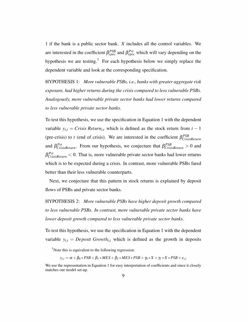
HYPOTHESIS 1: More vulnerable PSBs, i.e., banks with greater aggregate risk
exposure, had higher returns during the crisis compared to less vulnerable PSBs.
Analogously, more vulnerable private sector banks had lower returns compared
to less vulnerable private sector banks.
To test this hypothesis, we use the specification in Equation 1 with the dependent
variable yi,t = Crisis Returni,t which is defined as the stock return from t − 1
(pre-crisis) to t (end of crisis). We are interested in the coefficient β PSBCrisisReturn
and β PvtCrisisReturn. From our hypothesis, we conjecture that β PSB
CrisisReturn > 0 and
β PvtCrisisReturn < 0. That is, more vulnerable private sector banks had lower returns
which is to be expected during a crisis. In contrast, more vulnerable PSBs fared
better than their less vulnerable counterparts.
Next, we conjecture that this pattern in stock returns is explained by deposit
flows of PSBs and private sector banks.
HYPOTHESIS 2: More vulnerable PSBs have higher deposit growth compared
to less vulnerable PSBs. In contrast, more vulnerable private sector banks have
lower deposit growth compared to less vulnerable private sector banks.
To test this hypothesis, we use the specification in Equation 1 with the dependent
variable yi,t = Deposit Growthi,t which is defined as the growth in deposits
7Note this is equivalent to the following regression:
Development Bank of India (IDBI)) are publicly listed of which 21 are PSBs and
17 are private sector banks.
In our analysis, we use the Marginal Expected Shortfall (MES) to measure the
ex-ante vulnerability of public and private sector banks to an aggregate crisis.
The MES measure captures the tail dependence of the stock return of a financial
firm on the market as a whole. The strength of the measure lies in its ability
to predict which firms are likely to be worst affected when a financial crisis
materializes, as demonstrated by Acharya et al. (Forthcoming) in their analysis
of the systemic risk of large U.S. financial institutions around the financial crisis
of 2007–09.
Specifically, MES estimates the expected losses for a stock conditional on a
crisis. Since extreme tail events such as a mild financial crisis happen once a
decade and severe crisis such as the Great Depression or the Great Recession only
once in several decades, the practical implementation of MES relies on “normal”
tail events. We use the normal tail events as the worst 5 percent market outcomes
at daily frequency over the pre-crisis period. In our analysis, we take the 5
percent worst days for the market returns as measured by the S&P CNX NIFTY
index during the period of 1st January, 2007 to 31st December, 2007, and then
compute the negative of the average stock return for any given bank for these 511
percent worst days. As such, MES is a statistical measure but Acharya, Pedersen,
Philippon and Richardson (2010a) provide a theoretical justification for it in a
model where the financial sector’s risk-taking has externalities on the economy
whenever the sector as a whole is under-capitalized.8 In our baseline analysis
we use the MES as our measure of ex-ante risk. Our results are also robust to
alternate measures of risk (see Appendix D). Indian stock market data is from
the National Stock Exchange (NSE) and Bombay Stock Exchange (BSE). The
remaining variables and associated data sources used in our analysis in described
in Appendix B. Detail on the institutional environment and the time-line of how
the crisis progressed in India are provided in Appendix C.
II. Government Guarantees: Impact on Stock Returns
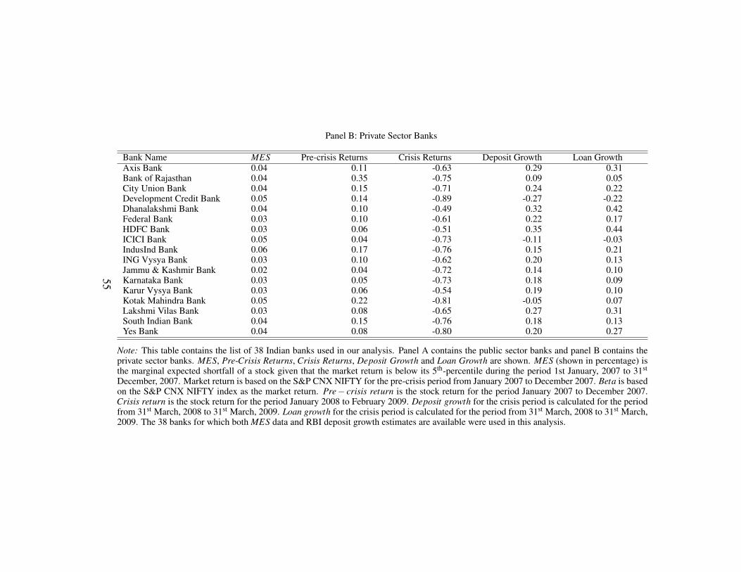
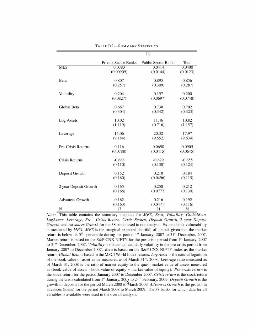
Table D2 in the appendix provides the summary statistics aggregated for all
38 banks and also aggregated separately for the 21 PSBs and 17 private sector
banks in our analysis. The significant loss of value for the bank stocks during
the crisis as suggested by the average realized return of -65.5 percent indicates
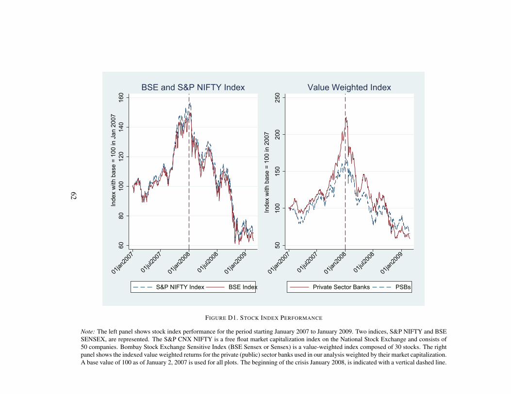
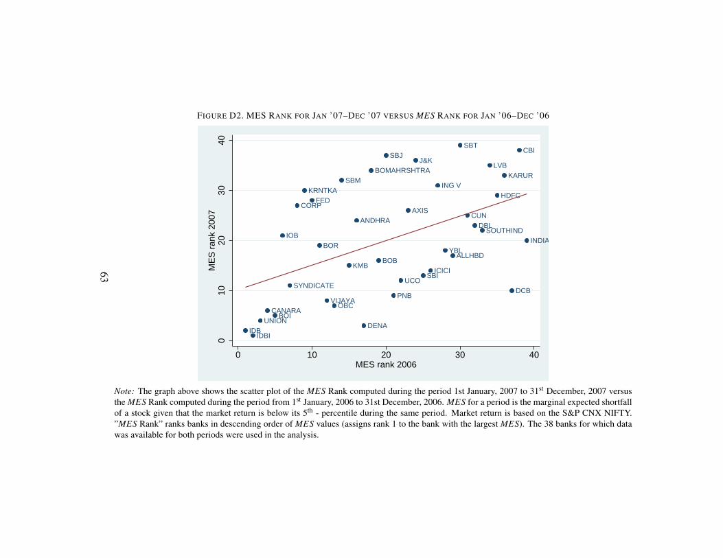
how trying this period was for the Indian banking industry as a whole. Figure D1
in the appendix shows that the stock market index — S&P CNX NIFTY index
— declined by nearly 60 percent from January 2008 to October 2008. Average
MES value measured in the pre-crisis period was 4.0 percent. What is important
for our analysis is whether a ranking of banks based on the normal-time MES
works well during the crisis. In Figure D2, we plot MES rankings from January
2006 -December 2006 against the MES ranks from January 2007 - December
2007 and show that MES rankings in 2006 were reflective of which banks would
8They show that the MES measure can be interpreted as one piece of the contribution of eachfinancial firm to the systemic risk in the event of a crisis, the other piece being the leverage of thefirm.
12
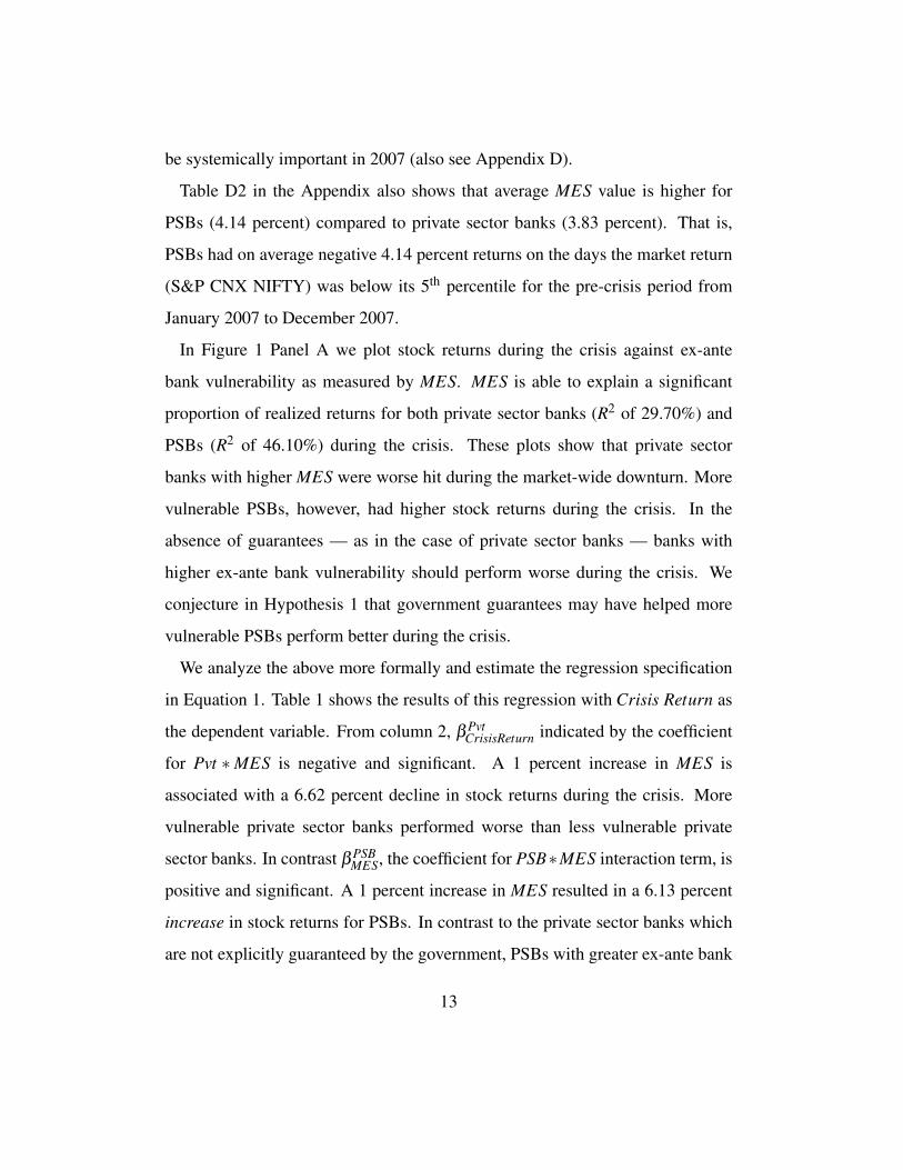
be systemically important in 2007 (also see Appendix D).
Table D2 in the Appendix also shows that average MES value is higher for
PSBs (4.14 percent) compared to private sector banks (3.83 percent). That is,
PSBs had on average negative 4.14 percent returns on the days the market return
(S&P CNX NIFTY) was below its 5th percentile for the pre-crisis period from
January 2007 to December 2007.
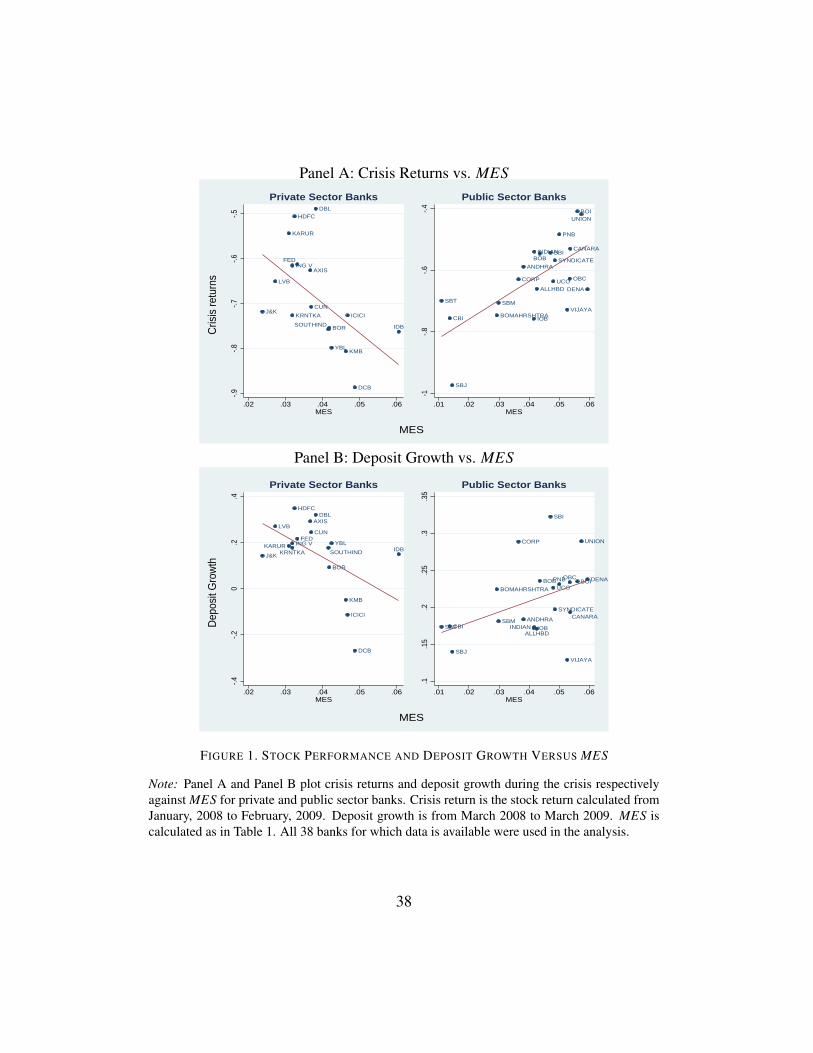
In Figure 1 Panel A we plot stock returns during the crisis against ex-ante
bank vulnerability as measured by MES. MES is able to explain a significant
proportion of realized returns for both private sector banks (R2 of 29.70%) and
PSBs (R2 of 46.10%) during the crisis. These plots show that private sector
banks with higher MES were worse hit during the market-wide downturn. More
vulnerable PSBs, however, had higher stock returns during the crisis. In the
absence of guarantees — as in the case of private sector banks — banks with
higher ex-ante bank vulnerability should perform worse during the crisis. We
conjecture in Hypothesis 1 that government guarantees may have helped more
vulnerable PSBs perform better during the crisis.
We analyze the above more formally and estimate the regression specification
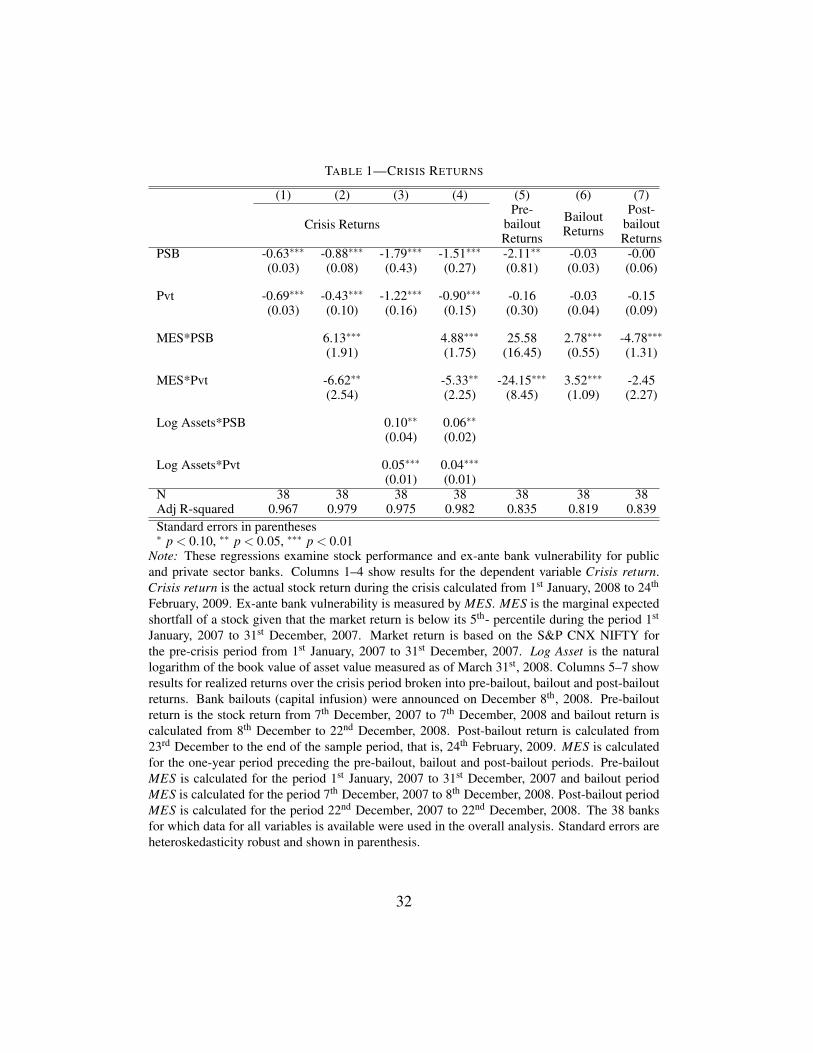
in Equation 1. Table 1 shows the results of this regression with Crisis Return as
the dependent variable. From column 2, β PvtCrisisReturn indicated by the coefficient
for Pvt ∗ MES is negative and significant. A 1 percent increase in MES is
associated with a 6.62 percent decline in stock returns during the crisis. More
vulnerable private sector banks performed worse than less vulnerable private
sector banks. In contrast β PSBMES, the coefficient for PSB∗MES interaction term, is
positive and significant. A 1 percent increase in MES resulted in a 6.13 percent
increase in stock returns for PSBs. In contrast to the private sector banks which
are not explicitly guaranteed by the government, PSBs with greater ex-ante bank
13
vulnerability outperformed less vulnerable PSBs.
One could argue that the more vulnerable PSBs were merely the largest banks
and thus what we are capturing is merely an implicit too-big-to-fail guarantee. In
column 3 we control for the size of the bank using Log Assets. Asset value is the
quasi- market value of assets measured as the difference in book value of assets
and book value of equity added to the market value of equity. Log Assets can
also be thought of as controlling for a too-big-to-fail guarantee. From column
3, we see that the larger banks performed better during the crisis. Since the
coefficient on the interaction term Log Assets ∗PSB is positive, we are assured
that the negative β PSBCrisisReturn is not entirely driven by a too-big-to-fail guarantee
for the larger PSBs.9 The pooled regression with both MES and Log assets show
similar results though with slightly lower magnitudes for the coefficients in both
bank categories.
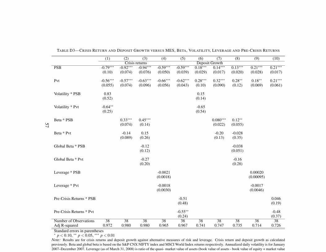
In Appendix D we also explore whether the “flight-to-quality” from private
sector banks to PSBs is due to the higher exposure of private sector banks to
global markets. Regression coefficients for a two factor model containing the
domestic market return and the global market return are shown in column 3 in
Table D3. The domestic beta coefficient measures sensitivity to the Indian NSE
stock market index whereas the global beta coefficient measures sensitivity to
the MSCI World market index. The coefficient for global beta is insignificant for
both public and private sector banks. Thus, the “flight-to-quality” from private
sector banks to PSBs does not seem to be due to differential exposure of more
vulnerable private sector banks to the global markets.
9Since PSBs tend to be on average larger than private sector banks (see Table D2) we cannotfully rule out that a too-big-to-fail guarantee played a role. Our model in Appendix A allows forany type of implicit or explicit guarantee. A too-big-to-fail guarantee in combination with thesebanks aggressively going after deposits can also yield the results in this paper. All we need toaccount for is that the most vulnerable banks were also not the biggest banks and the results forcolumn 4 show that our results are robust to this argument.
14
Columns 5–7 of Table 1 look at the impact of government guarantees on
stock returns as the crisis deepened. On December 8, 2008, the government of
India announced wide-ranging stimulus plans to jumpstart the banking system.
Specifically, PSBs were promised bailouts in the form of capital injections. We
examine bank returns around this announcement date. First, we divide our crisis
period into three sub-periods: pre-bailout (January 2008 to December 8, 2008),
bailout (2 week period following the announcement from December 8, 2008
to December 22, 2008), and post-bailout (December 23, 2008 to February 24,
2009).
From Table 1, column 5 we see that before the bailout announcement, more
vulnerable PSBs had higher returns whereas more vulnerable private sector banks
had lower returns. This can be potentially because the market expected the
government to step in only if a public sector bank failed. After the announcement
of the bailout, however, both vulnerable public and private sector banks had
higher returns (column 6). Since the announcement of capital infusion in PSBs
coincided with the announcement of a fiscal package, the market appears to
have priced in that private sector banks would also benefit from the stimulus
packages announced on December 8, 2008. That is, the market likely believed
that the fiscal package was substantial and would help the economy as a
whole. Post-bailout, specifically, after the two week period following the bailout
announcement, the relationship reverted to “normal” (column 7), that is, though
the coefficient for the interaction term with MES was negative for both public
and private sector banks, it is significant only for PSBs.
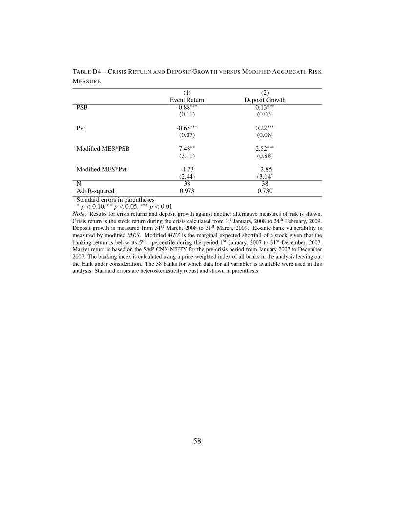
We conduct additional robustness checks in the appendix. In Table D4 in the
appendix, we show that our baseline results remain the same using a modified
version of the MES based on banking sector returns instead of the market index.
15
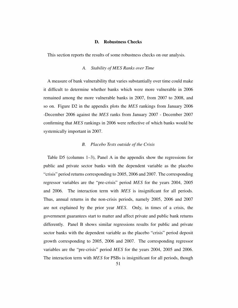
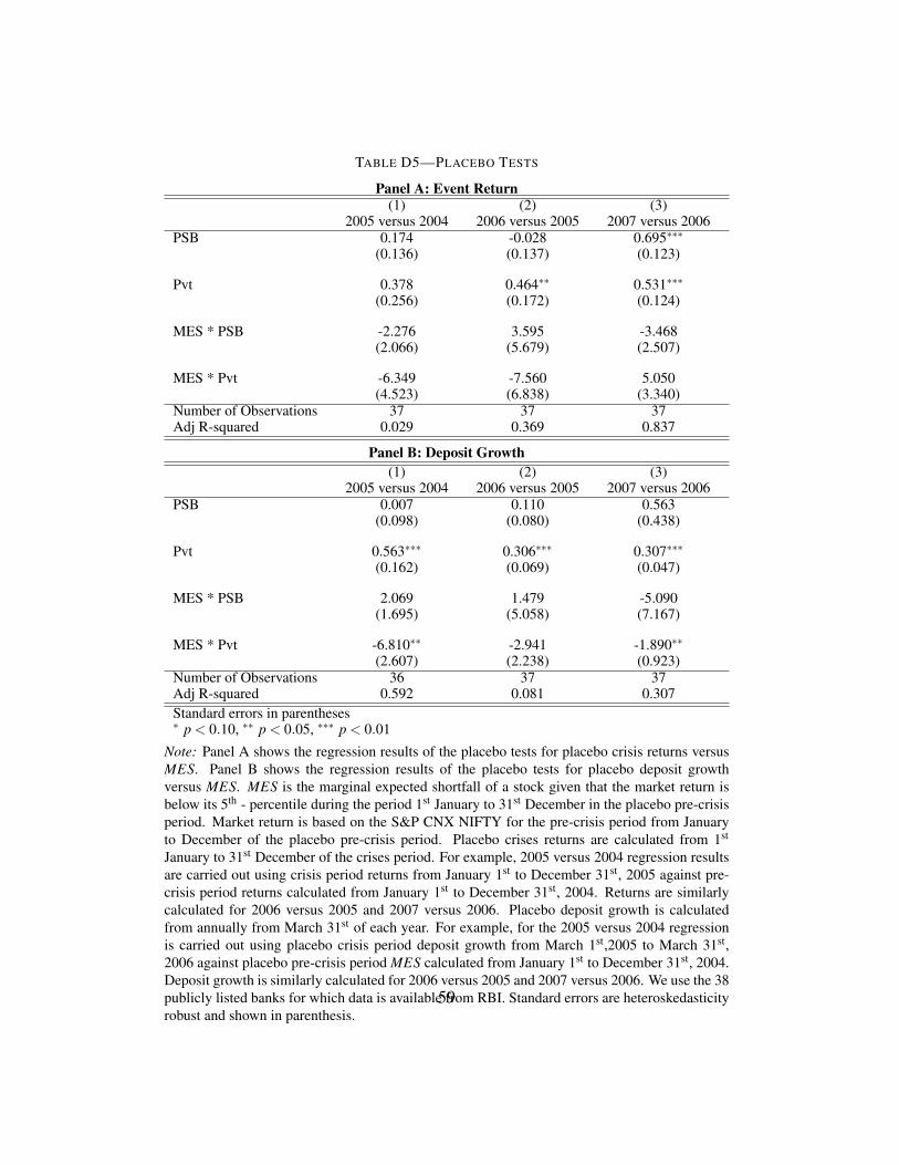
We conduct placebo tests using returns during placebo periods (non-crisis periods
being substituted for the crisis period) and do not find the differential effect on
public and private sector banks (see Table D5). Thus, only in times of a crisis do
government guarantees start to matter and affect private and public bank returns
differently. For further details, see Appendix D.
We documented so far the heterogeneity in crisis stock returns for private
and public sector banks and that bailouts appear to play a role in driving the
heterogeneity. Next, we explore whether this heterogeneity can be more directly
attributed to higher deposit growth of more vulnerable PSBs.
III. Impact on Deposits
We first look at deposit growth and then provide evidence for deposit rates.
A. Growth in Deposits
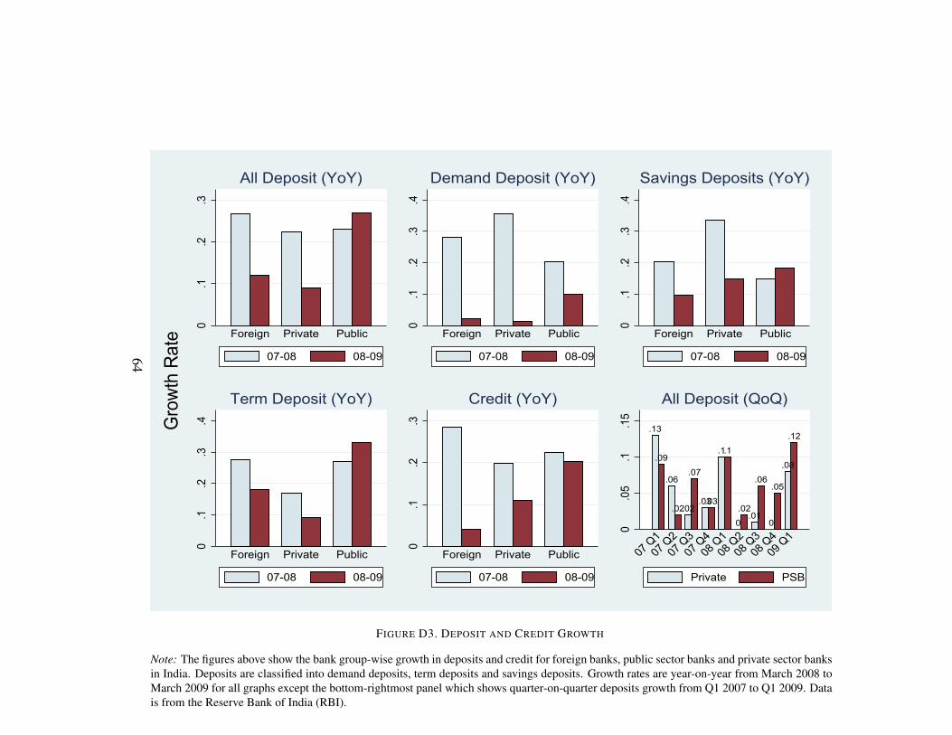
Growth in deposits for PSBs was strikingly different from that for private sector
banks during the crisis. While the banking sector as a whole experienced a
slowdown in deposit growth, private sector banks were affected to a larger extent
(see Figure D3). RBI estimates indicate that deposits of PSBs grew by 26.9
percent during the crisis (March 2008 to March 2009) compared to 23.1 percent
a year earlier (March 2007 to March 2008).10 In comparison, for private sector
banks deposit growth slowed from 22.3 percent to a mere 9.1 percent in the same
period. While the above estimates refer to all 50 banks for which data is provided
by RBI, the deposit growth also show similar patterns when we restrict to the
38 banks used in our analysis (see Table D2). Looking at this aggregated data
10Deposit data is provided by RBI annually for the period ending March 31st of each year.Hence the annual deposit growth is calculated from March of previous year to March of currentyear.
16
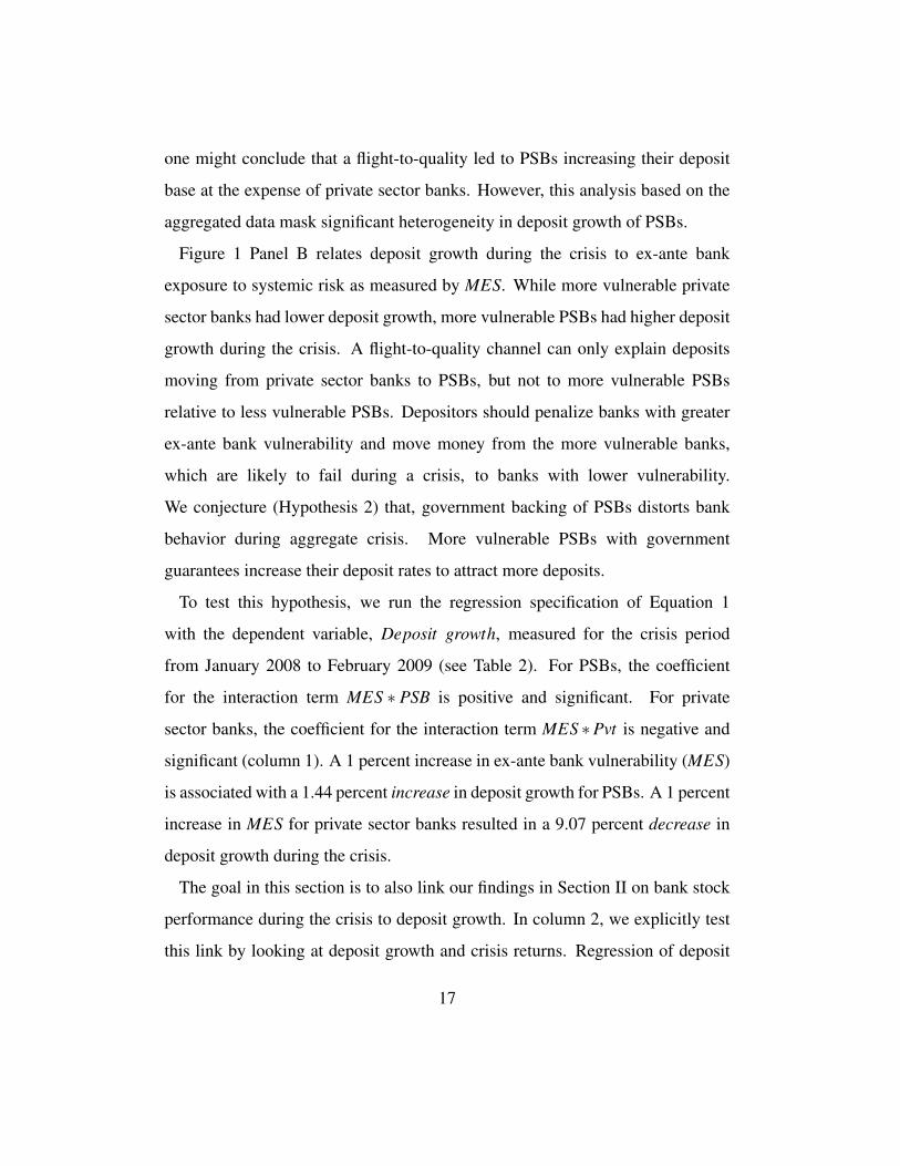
one might conclude that a flight-to-quality led to PSBs increasing their deposit
base at the expense of private sector banks. However, this analysis based on the
aggregated data mask significant heterogeneity in deposit growth of PSBs.
Figure 1 Panel B relates deposit growth during the crisis to ex-ante bank
exposure to systemic risk as measured by MES. While more vulnerable private
sector banks had lower deposit growth, more vulnerable PSBs had higher deposit
growth during the crisis. A flight-to-quality channel can only explain deposits
moving from private sector banks to PSBs, but not to more vulnerable PSBs
relative to less vulnerable PSBs. Depositors should penalize banks with greater
ex-ante bank vulnerability and move money from the more vulnerable banks,
which are likely to fail during a crisis, to banks with lower vulnerability.
We conjecture (Hypothesis 2) that, government backing of PSBs distorts bank
behavior during aggregate crisis. More vulnerable PSBs with government
guarantees increase their deposit rates to attract more deposits.
To test this hypothesis, we run the regression specification of Equation 1
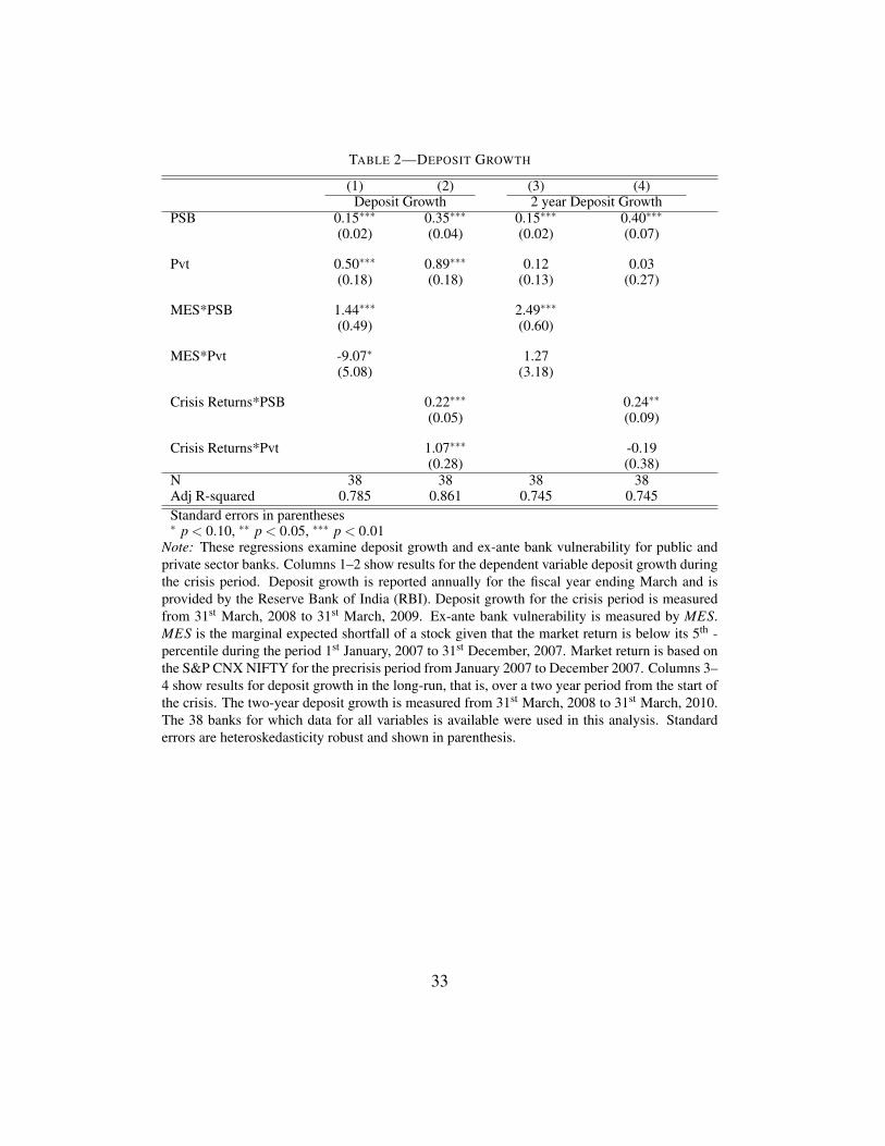
with the dependent variable, Deposit growth, measured for the crisis period
from January 2008 to February 2009 (see Table 2). For PSBs, the coefficient
for the interaction term MES ∗ PSB is positive and significant. For private
sector banks, the coefficient for the interaction term MES ∗Pvt is negative and
significant (column 1). A 1 percent increase in ex-ante bank vulnerability (MES)
is associated with a 1.44 percent increase in deposit growth for PSBs. A 1 percent
increase in MES for private sector banks resulted in a 9.07 percent decrease in
deposit growth during the crisis.
The goal in this section is to also link our findings in Section II on bank stock
performance during the crisis to deposit growth. In column 2, we explicitly test
this link by looking at deposit growth and crisis returns. Regression of deposit
17
growth against crisis returns shows that, both public and private sector banks
with higher crisis returns had higher deposit growth in line with our hypothesis.
Paralleling our analysis on event returns in Section II on pre-bailout, bailout and
post-bailout trends, we would like to see the patterns in deposit growth as the
crisis progressed. Since RBI publishes only aggregate data for deposit growth at
the quarterly frequency, we analyze deposit growth as the crisis deepened only at
the aggregate level. Thus, the data is for all 50 public and private sector banks in
India (as opposed to the 38 publicly listed banks that are used in our analysis).
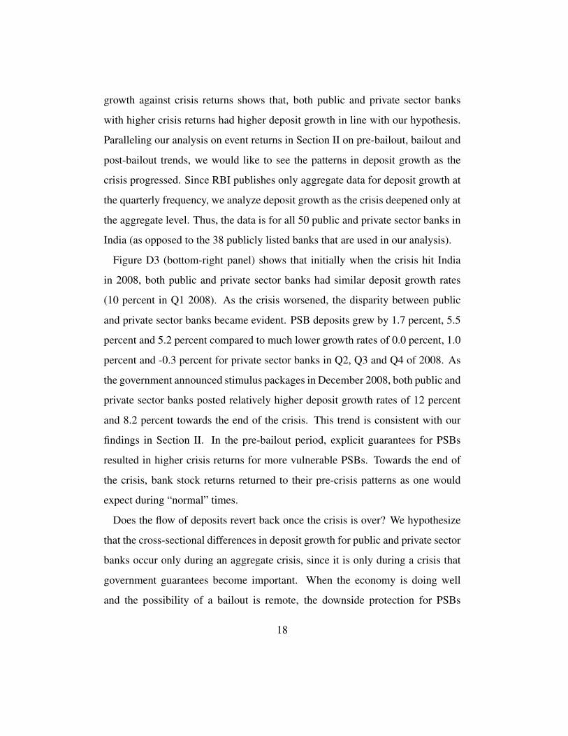
Figure D3 (bottom-right panel) shows that initially when the crisis hit India
in 2008, both public and private sector banks had similar deposit growth rates
(10 percent in Q1 2008). As the crisis worsened, the disparity between public
and private sector banks became evident. PSB deposits grew by 1.7 percent, 5.5
percent and 5.2 percent compared to much lower growth rates of 0.0 percent, 1.0
percent and -0.3 percent for private sector banks in Q2, Q3 and Q4 of 2008. As
the government announced stimulus packages in December 2008, both public and
and 8.2 percent towards the end of the crisis. This trend is consistent with our
findings in Section II. In the pre-bailout period, explicit guarantees for PSBs
resulted in higher crisis returns for more vulnerable PSBs. Towards the end of
the crisis, bank stock returns returned to their pre-crisis patterns as one would
expect during “normal” times.
Does the flow of deposits revert back once the crisis is over? We hypothesize
that the cross-sectional differences in deposit growth for public and private sector
banks occur only during an aggregate crisis, since it is only during a crisis that
government guarantees become important. When the economy is doing well
and the possibility of a bailout is remote, the downside protection for PSBs
18
is essentially immaterial. Thus, deposit growth for both vulnerable public and
private sector banks should show the same pattern in normal times.11 Columns 2–
4 in Table 2 confirm this intuition. Deposit growth is for the two year period from
March 2008 to March 2010. The coefficient for the interaction term MES∗Pvt is
insignificant while the coefficient for the interaction term MES ∗PSB is positive
and significant (2.49) for PSBs. The two-year period includes both a crisis period
and a non-crisis period. For high MES private sector banks, deposits fell during
the crisis period but grew during the non-crisis period. In contrast, for high MES
PSBs, deposits grew during both crisis and non-crisis periods. These results point
to another interesting fact: crisis time guarantees result in a permanent shift in
deposits from private sector banks to PSBs. Deposits gained by PSBs during the
crisis do not revert in the period following the crisis suggesting that guarantees
during times of crisis have long-term effects on bank health.12
B. Deposit Rates
INDIRECT EVIDENCE
Why did depositors move deposits to the more vulnerable PSBs and not to
the safer PSBs? Did vulnerable PSBs increase their deposit rates to attract
deposits? Ideally, we would like to look at individual-level deposit data and see
whether more vulnerable PSBs indeed increased deposit rates during the crisis.
However, since RBI does not provide this information, we exploit heterogeneity
in government regulation of deposit rates across deposits of different types to test
the link between deposit rates and growth in deposits. We first provide evidence
11In our model in Section A, we explicitly make the assumption that government guaranteesplay no role in the idiosyncratic state. There is no asymmetry between public and private sectorbanks in this non-crisis state and government guarantees play no role.
12This is consistent with Iyer and Puri (2012) who find that depositors that run on the Indianbank in their analysis do not return back to the bank once the bank run is over.
19
exploiting this heterogeneity. We supplement this analysis by also providing
direct evidence from bank-level deposit rate data.
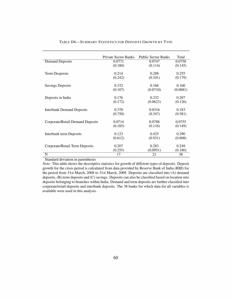
Deposits can be classified into a) demand deposits; b) savings bank deposits;
and, c) term deposits. Demand deposits, which account for 11 percent of all
deposits, are short maturity deposits and are withdrawable on demand. Saving
deposits, which account for 20 percent of all deposits, are a form of demand
deposit and are subject to restrictions on withdrawals. Term deposits, which
account for the majority (69 percent) of all deposits, are for a fixed period
typically longer than the maturity of demand deposits. One important distinction
between these different deposit types is that while banks can set deposit rates for
demand deposits and term deposits, savings deposit rates during this period were
heavily regulated by the government.13 We exploit this difference in regulation
of deposit rates to determine whether banks were actively increasing deposit rates
to attract deposits. Heavy regulation of savings deposits did not allow banks to
change deposit rates. In contrast, banks could potentially change deposit rates
for term and demand deposits.
Demand deposits grew on average at a slightly higher 7.71 percent for private
sector banks compared to 7.47 percent for PSBs (see Table D6). Average growth
rate for term deposits was higher for PSBs (28.8 percent) compared to private
sector banks (21.4 percent). This difference is consistent with the conjecture
that depositors perceived private sector banks to be more vulnerable and shifted
deposits to the lower maturity demand deposits whereas for PSBs depositors
shifted to the higher maturity term deposits in line with a flight-to-quality story.
The growth rate of savings deposits was higher for PSBs (16.6 percent) relative
13It was only after October 2011 that savings deposits were deregulated and banks wereable to change deposit rates (see “Deregulation of Savings Bank Deposit Interest Rate -Guidelines”, October 25, 2011 https://www.rbi.org.in/scripts/NotificationUser.aspx?Id=6779&Mode=0).
20
to private sector banks (15.2 percent).
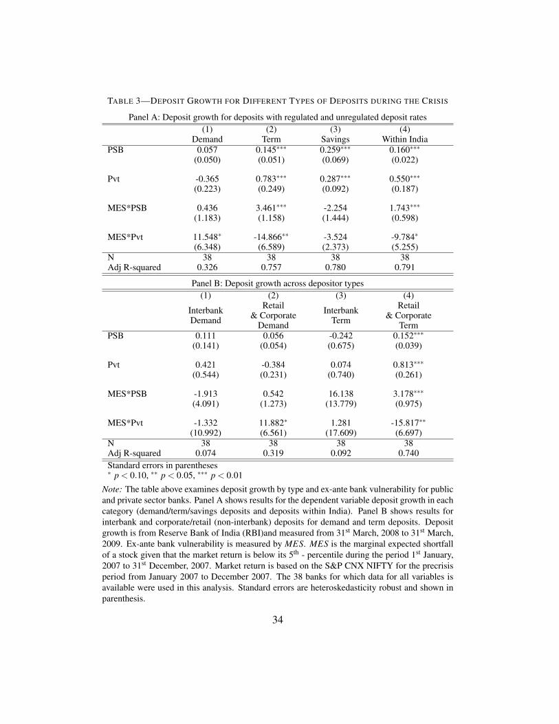
Table 3 shows the regression results for Equation 1 with the dependent variable
as the growth rate of deposits for each category. Demand deposit growth for
private sector banks is higher for banks with higher MES. In contrast, the
relationship between MES and demand deposit growth is weak for PSBs as they
did not experience a similar shortening of deposit maturity. On breaking down
demand deposits further into inter-bank and corporate/retail deposits (Panel B),
we see that the growth in demand deposits for private sector banks is driven by
the corporate/retail sector. In column 2 of Panel A, with growth in term deposits
as the dependent variable, we see the familiar result — more vulnerable PSBs
had higher term deposit growth whereas more vulnerable private sector banks
had lower term deposit growth. Further, the effect in term deposits is driven
by corporate and retail deposits (column 4, Panel B). Inter-bank term deposits
(column 3, Panel B), however, do not show the same pattern. Troubled banks
would like to borrow the most in a crisis at longer maturities, e.g., by offering
higher term deposit rates. Since inter-bank lending tends to be at the short end,
we see a weaker relationship in these shorter-term maturities. Overall, the above
results indicate that depositors were shifting away from term (longer maturity)
deposits at more vulnerable private sector banks to demand (shorter maturity)
deposits. On the other hand, PSBs witnessed deposit growth in the more stable
longer maturity term deposits.
Savings deposits growth (column 3, Panel A) does not exhibit a positive
relation with MES for PSBs. In fact for savings deposits, the coefficient for
the MES∗PSB and MES∗Pvt interaction terms are insignificant for both public
and private sector banks. Since savings deposit rates are set by the government
of India, the more vulnerable PSBs cannot increase their deposit rates to attract
21
deposits. Thus, the relationship for savings deposit growth with MES is the same
for both public and private sector banks as one would expect if PSBs did not
change their deposit rates.
Lastly in column 4 of Panel A we look at deposits within India. Banks can set
rates only for deposits within India whereas deposits rates for deposits outside
India are regulated by the RBI. Consistent with our hypothesis, for deposits
in branches within India, the coefficient of the interaction term MES ∗PSB is
positive and significant while the coeffcient for the interaction term MES ∗Pvt
is negative and significant. For deposits outside India (not shown), we do not
observe the same pattern.
SOME DIRECT EVIDENCE
We now turn to average bank-level deposit rate data to show that banks did
indeed increase their deposit rates as the crisis progressed. We have deposit rates
only at the bank-level and the data is not disaggregated at the individual level.
Short-term deposits are deposits with maturity less than three years and long-
term deposits have maturities greater than three years. This data is not publicly
available and has been provided to us by RBI for each bank at the quarterly
frequency beginning March 2008. We use the average of the maximum and
minimum values of the deposit rate for each bank in each quarter.
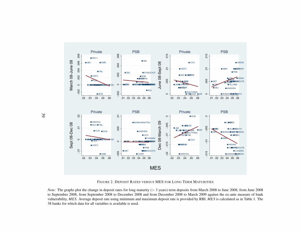
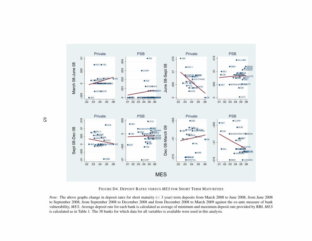
Figure 2 and Figure D4 provide the change in deposit rates for long-term
maturities and short-term maturities respectively, in each quarter of the crisis
against ex-ante bank vulnerability, i.e. MES. We observe an interesting trend
as the crisis progressed. Between June 2008 and September 2009, deposit
rates decreased for more vulnerable private sector banks and increased for more
vulnerable PSBs. This effect is more evident for the long-term deposits (Figure 2,22
top-right). It is only towards the end of the crisis that PSBs were in fact cutting
deposit rates. Again, this effect is more evident for long-term deposits (Figure 2,
bottom-right).14
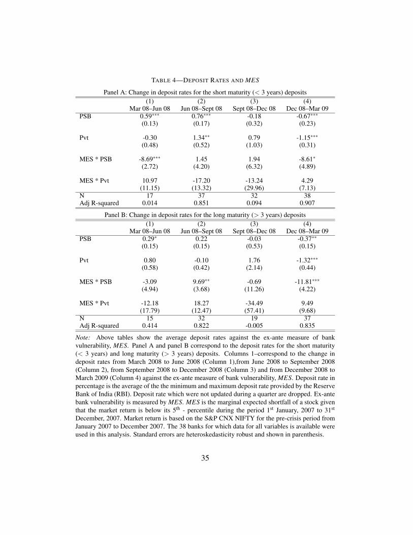
Table 4 confirms our results with formal regressions. In these regressions, we
drop data points which were likely not updated. That is, we drop data points
where quarter-on-quarter changes were zero. From Panel A, we see that more
vulnerable private sector banks did not significantly change deposit rates for
short-term deposits. More vulnerable PSBs on the other hand decreased deposit
rates in the beginning (Panel A, column 1) and towards the end of the crisis (Panel
A, column 4). This is consistent with the previous section where we found that
more vulnerable PSBs did not have significant deposit growth for the shorter-
term deposits. In column 2 of Panel B, however, as the crisis deepened in Q3
2008, more vulnerable PSBs increased deposit rates for long-term deposits from
June 2008 to September 2008. Towards the end of the crisis, more vulnerable
PSBs started decreasing their deposit rates (Panel B, column 4) for long-term
deposits too.15 Finally, we conduct several robustness checks (see Appendix D)
to show that our results are robust to alternate measures of MES and to placebo
crisis periods.
Our analysis in this section shows that deposits shifted from private sector
banks to PSBs in the crisis period. By exploiting a regulatory policy, which
allowed banks to change deposit rates of only certain kinds of deposits, we show
that more vulnerable PSBs likely increased deposit rates. We also provide direct
14Note, however, due to the poor quality of data, many of the changes in deposit rates are zeroespecially for changes between March 2008 and June 2008 and between September 2008 andDecember 2008.
15Consistent with this effect of government guarantees on deposits, Acharya and Mora (2015)find that during the financial crisis of 2007–08, riskier commercial banks in the United Statesmanaged to attract more federally-insured deposits by offering higher rates even as they wereexperiencing a slow “run” (reduction in quantities as well as shortening of maturity) of uninsureddeposits.
23
evidence using aggregated deposit rates that more vulnerable PSBs were indeed
increasing deposit rates to attract deposit outflow from the private sector banks.
IV. Impact on Bank Lending
We now examine whether the increased flow of deposits into PSBs translated
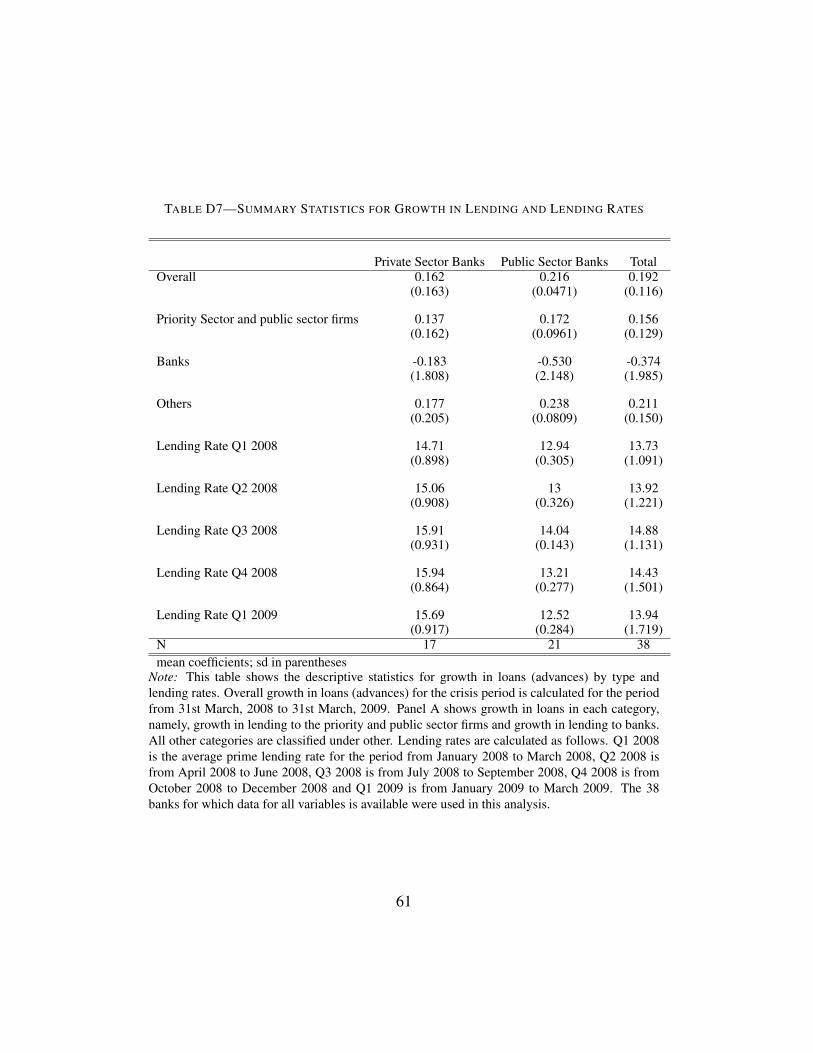
into an increased flow of credit to the real economy. In line with the higher
deposit growth for PSBs in Section III, we find that credit did indeed grow at a
higher 21.6 percent for PSBs compared to 16.2 percent for private sector banks
during the crisis (see Table D7).
There are several reasons why state-owned banks may not cut back on lending
during crises. One argument is that vulnerable PSBs are socially maximizing
and therefore increase lending during crises and are thus helpful in maintaining
credit flow in the economy during crises periods. In contrast, a political economy
view suggests that political pressure leads to public sector banks lending during
crises but may also result in funding of inefficient investments. Both the social
motive and the political motive result in greater lending and subsequently higher
investment. The difference, however, is that in the former, state-owned banks
invest in projects which are welfare maximizing whereas in the latter the state-
owned banks invest in inefficient projects based on political motives. To see
which of the above motives were responsible for increased lending by banks we
turn to the data. We examine the impact of crisis time guarantees on both the
amount of lending as well as on bank lending rates.16
16The “lazy banking” theory (Banerjee, Cole and Duflo (2005)) says that managers of state-owned banks face an asymmetric incentive structure wherein they are penalized for making badloans but do not face harsh consequences for passing on good opportunities. At face value, sincePSBs increased lending our results seem to suggest that a “lazy banking” theory (Banerjee, Coleand Duflo (2005)) may not be at play. However, it could be that loan managers are more prone toincrease lending to existing customers and thus, we see an increase in lending to the politicallyimportant sectors. This distinction is not important for our analysis. What matters is how theseloans performed in the aftermath of the crisis and whether they were the more economically
24
A. Bank Lending
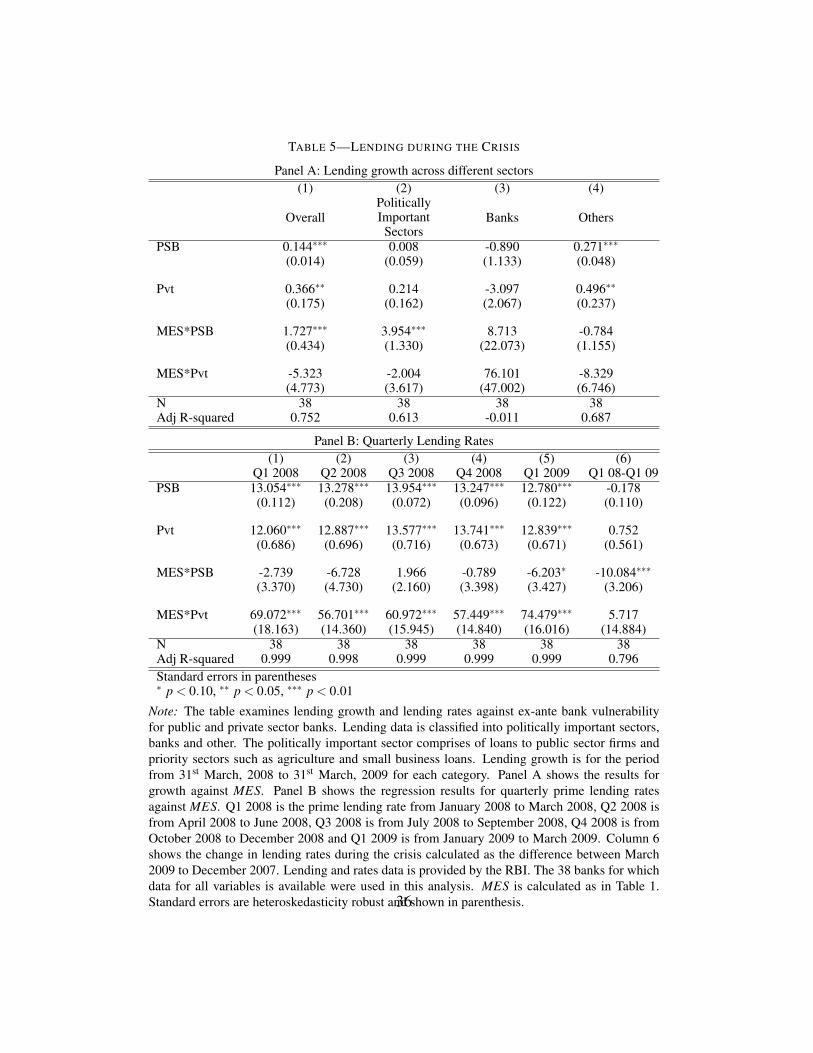
Column 1 of Table 5 indicates that more vulnerable PSBs did indeed increase
lending during the crisis. A 1 percent increase in ex-ante bank vulnerability as
measured by MES is associated with a 1.73 percent increase in lending. We next
look at what sectors drive this higher lending by the PSBs. In columns 2–4 we
split loan growth into lending to (i) politically important sectors; (ii) banks; and a
catch-all category (iii) other. The politically important sector comprises of loans
to public sector firms and to the priority sector which includes agriculture and
small businesses loans. Our results indicate that the increase in lending by the
vulnerable PSBs is driven by lending to politically important sectors. In column
2, we see that a 1 percent increase in ex-ante bank vulnerability, MES, resulted
in a 3.95 percent increase in lending by PSBs to the politically important sector.
More vulnerable private sector banks, on the other hand, did not significantly
increase lending to these politically important sectors.
B. Lending Rates
In Section III, we established that vulnerable PSBs experienced an increased
inflow of deposits possibly by increasing their deposit rates. In this section, we
examine whether this higher cost of funding — higher deposit rates — translated
into higher lending rates on loans for PSBs. Panel B of Table 5 shows that more
vulnerable private sector banks had significantly higher lending rates throughout
the crisis from Q1 2008 to Q1 2009. More vulnerable PSBs which raised their
deposit rates and had higher borrowing costs, however, did not have similar
higher lending rates. Column 5 of Panel B, Table 5 shows that lending rates
were in fact 6 basis points lower for more vulnerable PSBs in Q1 2009 as the
viable projects.25
coefficient on the interaction term for MES ∗PSB indicates. Column 6 looks at
the change in lending rates from Q1 2008 to Q1 2009. More vulnerable PSBs
decreased lending rates by 10 basis points after the onset of the crisis.
More vulnerable PSBs potentially did not care about higher deposit rates eating
into their profit margins because they would be bailed out by the government in
the worst case. But one could argue that the effect of higher deposit rates is not
so severe since both consumers and the real economy benefit — consumers get
higher deposit rates and at the same time firms are not penalized with higher
lending rates. We find, however, that PSBs were lending mostly to the priority
and public sectors which are of particular interest to the government. The
findings in this section are consistent with the political economy view mentioned
previously. While these political interests may result in increased lending, this
might not necessarily be maximizing social welfare as the politically motivated
lending may result in inefficient investments. Next, we look at the impact of this
lack of market discipline on the long-term performance of loans.
V. Loan Performance and Capital Injections
We now look at non-performing assets (NPAs) and restructured loans in the
aftermath of the crisis from March 2008 to March 2015. Loans are classified as
NPA if a borrower misses payments for 90 days (or 180 days in some cases).
Restructuring of loans modifies the terms of existing loans if the lender deems
the borrower is unable to repay the loan. Banks are less inclined to recognize bad
loans and more prone to restructure assets which allows them to not recognize
losses on bad loans first. Hence we focus on both NPAs and restructing of assets.
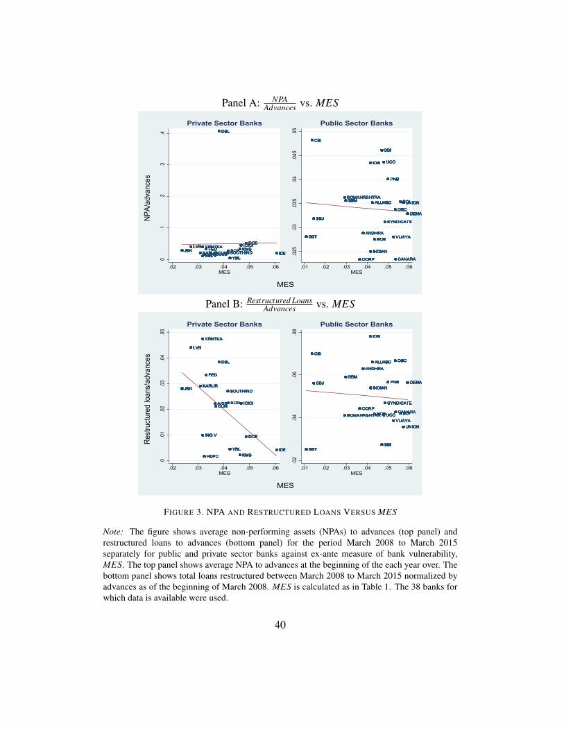
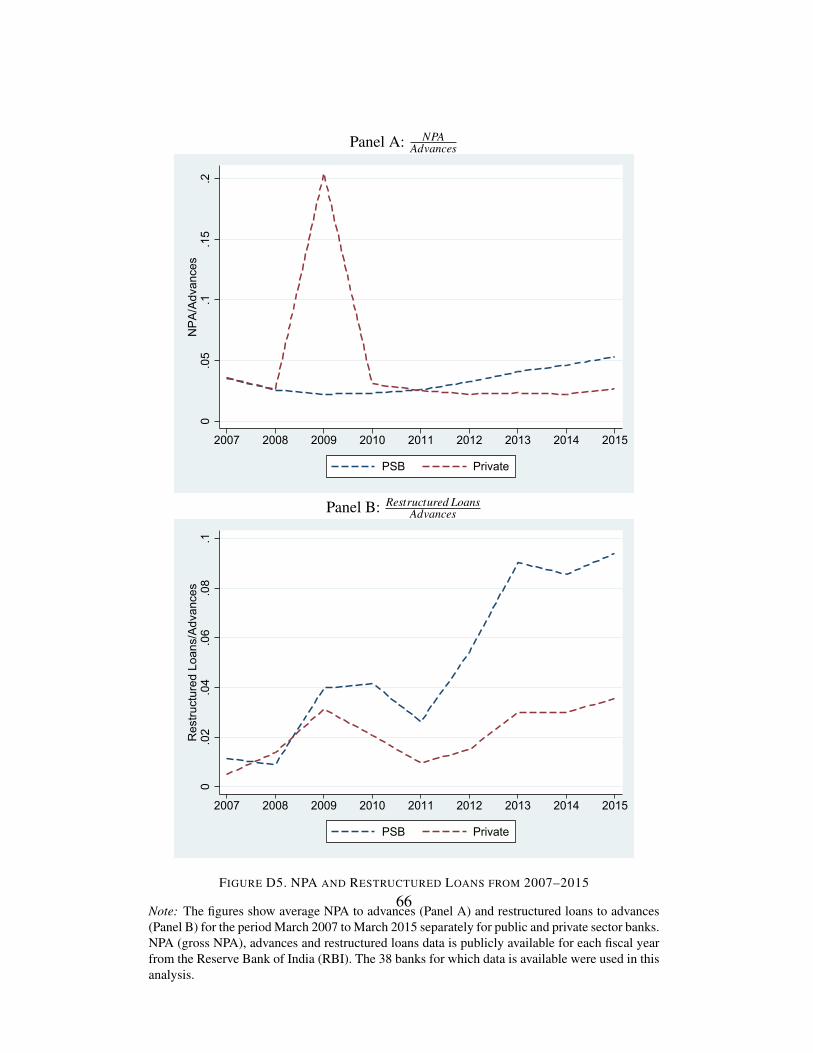
Following the crisis, the NPA to total loan advances remained relatively stable
for PSBs throughout the period whereas private sector banks had a spike in their26
NPAs in the period immediately following the crisis but have had lower overall
NPAs since then (Figure D5, Panel A). Restructured loans as a percentage of loan
advances rose for both private and public sector banks but rise was more stark for
PSBs (Figure D5, Panel B).17 On examining the cross-sectional heterogeneity
against ex-ante bank vulnerability, we see that MES and NPAs are not correlated
(Figure 3).18 However, more vulnerable private sector banks had on average
starkly lower restructurings (Figure 3).
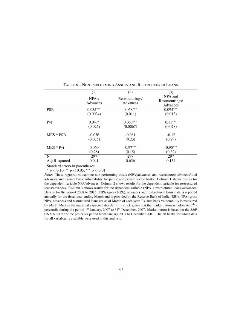
More formal regressions in Table 6 shows similar results. Ex-ante bank
vulnerability and NPAs to loan advances are not significantly related (column
1). However, private sector banks with greater ex-ante bank vulnerability had
lower restructured loans (column 2). More vulnerable private sector banks had
1 percent lower ratio of restructured loans to loan advances. This might be
attributable to the more prudent lending by the vulnerable private sector banks
in contrast to vulnerable PSBs which increased lending to politically important
sectors and at lower loan rates. We do not see any effect on the NPAs of
PSBs probably because they are reluctant to recongnize bad loans.19 Hence,
we interpret the lower NPAs of more vulnerable private sector banks as the true
counterfactual wherein the market disciplines banks resulting in more prudent
lending. Lack of such market discipline in the case of PSBs implies that we do
17Note Bank of Rajasthan was merged with ICICI in 2010. Results are qualitatively similar ifwe drop these banks from the analysis.
18When we restrict to agricultural NPAs, we do see that more vulnerable PSBs had higheragricultural NPAs with a one percent higher MES corresponding to a 36 percent higheragricultural NPAs to total advances to the agricultural sector. There was no effect on the privatesector banks. Since this is likely driven by a large debt waiver program announced by thegovernment in 2008 (see Mukherjee, Subramanian and Tantri (2014), Gine and Kanz (2014)),we focus on the restructured loans.
19The process of recognizing NPAs and bank balance sheet clean-up is still on-going. The process of forcing PSBs to recognize bad loans on their balance sheetsis still on-going and thus may mask true health of these loans (See “Bank NPAs mayhit 8.5 % by March ”, June 28 2016, http://www.thehindu.com/business/Economy/financial-stability-report-released/article8784187.ece)
27
not observe similar lowering of restructured loans for PSBs.
VI. Capital Injections in PSBs
Next, we look at the extent of capital support provided by the Indian
government to the PSBs in the aftermath of the crisis as a direct measure of
government support received by different banks. Since the sample of banks that
received capital injections is small, we only provide a descriptive study. Evidence
suggests that weaker PSBs received greater capital injections. Beginning
December 2008, the government announced a number of capital injections for
PSBs. In February 2009, the government announced capital injections in 3
PSBs: UCO Bank, Central Bank of India and Vijaya Bank. Further, as part
of the 2010-2011 budget, the government announced additional capital infusion
in five PSBs: IDBI Bank, Central Bank, Bank of Maharashtra, UCO Bank and
Union Bank. The amount of capital injections was determined based on PSB
funding requirements and the need for a capital buffer. Effectively, the PSBs
which performed the worst during the crisis resulting in high capital depletion
were more likely to receive support from the government. As of March 2009, all
the banks mentioned above (except Union Bank) had less than 8 percent of Tier 1
capital. Based on the MES measure, these were also among the more vulnerable
banks in our analysis. For example, Union Bank had an MES of 5.74 percent
and Vijaya Bank had an MES of 5.27 percent. UCO Bank had a relatively lower
MES of 4.80 percent. In summary, more vulnerable PSBs did receive greater
ex-post government support. Such direct capital support was not provided to
more vulnerable private sector banks, consistent with our starting assumption
that PSBs have greater government support compared to the private sector banks.28
VII. Conclusion
In this paper, we examine the relatively strong performance of state-owned
banks in India compared to their private-sector counterparts during the global
financial crisis of 2007–09. While more vulnerable private sector banks
performed worse than less vulnerable private sector banks, vulnerable state-
owned banks performed better. We attribute this to the presence of government
guarantees which enabled more vulnerable state-owned banks to grow their
deposit base by increasing their deposit rates. While they also increased loan
advances, they did so at cheaper rates and especially to politically important
sectors. Ex-post, these loan advances have been associated with greater non-
performance and restructuring of assets, thus sowing the seeds of an economic
slowdown in investments in India (as documented in Acharya, Mishra and
Prabhala (2005)).
Our findings are, in fact, consistent with the experience worldwide: financial
institutions with greater access to government guarantees have survived the crisis
or even expanded post-crisis while the ones without such access have failed
or shrunk. A striking case in point has been the growth of the government-
sponsored enterprises (Fannie Mae and Freddie Mac) and commercial banks in
the United States - both sets of institutions with explicit government support and
ready access to central bank emergency lending. These institutions expanded
their holdings of mortgage-backed securities while investment banks and hedge
funds deleveraged and sold these securities (He, Khang and Krishnamurthy
(2010)). Eventually, Fannie Mae and Freddie Mac effectively failed and were put
under the United States government conservatorship in September 2008. Thus,
even though access to government guarantees might be considered a source of
financial stability during a crisis, our results suggest that greater presence of29
government institutions in the financial sector (or greater extent of government
intervention in a crisis) is likely to be associated with the misfortune of crowding
out the private financial sector in the long run.
REFERENCES
Acharya, Viral, and Nada Mora. 2015. “A Crisis of Banks as Liquidity
Providers.” Journal of Finance.
Acharya, Viral, D. Anginer, and A.J. Warburton. 2014. “The End of Market
Discipline? Investor Expectations of Implicit State Guarantees.” NYU Stern
School of Business, Working Paper.
Acharya, Viral, Prachi Mishra, and N.R. Prabhala. 2005. “Bank Financing in
India.” Working paper, CAFRAL.
Acharya, Viral V., Lasse Heje Pedersen, Thomas Philippon, and Matthew P.
Richardson. Forthcoming. “Measuring Systemic Risk.” Review of Financial
Studies.
Banerjee, Abhijit, Shawn Cole, and Esther Duflo. 2005. “Bank Financing
in India.” India’s and China’s Recent Experience with Reform and Growth,
Wanda Tseng and David Cowen, eds.
Calomiris, Charles W., and Stephen H. Haber. 2009. Fragile by Design: The
Political Origins of Banking Crises and Scarce Credit.
Cordella, T., and E. Yeyati. 2003. “Bank bailouts: Moral Hazard vs. Value
Effect.” Journal of Financial Intermediation, 12: 300–330.
Gine, Xavier, and Martin Kanz. 2014. “The Economic Effects of a Borrower
Bailout: Evidence from an Emerging Market.” Working paper.30
Gorton, G., and L. Huang. 2004. “Liquidity, Efficiency and Bank Bailouts.”
American Economic Review, 94: 455–83.
Gropp, Reint, Jukka Vesala, and Giuseppe Vulpes. 2004. “Equity and Bond
Market Signals as Leading Indicators of Bank Fragility.” Journal of Money,
Credit and Banking, 38: 399–428.
He, Zhiguo, In Gu Khang, and Arvind Krishnamurthy. 2010. “ Balance Sheet
Adjustments in the 2008 Crisis.” IMF Economic Review, 58: 118–156.
Iyer, Rajkamal, and Manju Puri. 2012. “Understanding Bank Runs :
The Importance of Depositor-bank Relationships and Networks.” American
Economic Review, 102(4): 1414–1445.
Micco, Alejandro, and Ugo Panizza. 2006. “Bank ownership and lending
behavior.” Economics Letters, 93: 248 – 254.
Mukherjee, Saptarshi, Krishnamurthy Subramanian, and Prasanna Tantri.
2014. “Costs and Benefits of Debt Moratoria: Evidence from a Natural
Experiment in India.” Working paper.
Sapienza, Paola. 2004. “The effects of government ownership on bank lending.”
N 38 38 38 38 38 38 38Adj R-squared 0.967 0.979 0.975 0.982 0.835 0.819 0.839Standard errors in parentheses∗ p < 0.10, ∗∗ p < 0.05, ∗∗∗ p < 0.01
Note: These regressions examine stock performance and ex-ante bank vulnerability for publicand private sector banks. Columns 1–4 show results for the dependent variable Crisis return.Crisis return is the actual stock return during the crisis calculated from 1st January, 2008 to 24th
February, 2009. Ex-ante bank vulnerability is measured by MES. MES is the marginal expectedshortfall of a stock given that the market return is below its 5th- percentile during the period 1st
January, 2007 to 31st December, 2007. Market return is based on the S&P CNX NIFTY forthe pre-crisis period from 1st January, 2007 to 31st December, 2007. Log Asset is the naturallogarithm of the book value of asset value measured as of March 31st, 2008. Columns 5–7 showresults for realized returns over the crisis period broken into pre-bailout, bailout and post-bailoutreturns. Bank bailouts (capital infusion) were announced on December 8th, 2008. Pre-bailoutreturn is the stock return from 7th December, 2007 to 7th December, 2008 and bailout return iscalculated from 8th December to 22nd December, 2008. Post-bailout return is calculated from23rd December to the end of the sample period, that is, 24th February, 2009. MES is calculatedfor the one-year period preceding the pre-bailout, bailout and post-bailout periods. Pre-bailoutMES is calculated for the period 1st January, 2007 to 31st December, 2007 and bailout periodMES is calculated for the period 7th December, 2007 to 8th December, 2008. Post-bailout periodMES is calculated for the period 22nd December, 2007 to 22nd December, 2008. The 38 banksfor which data for all variables is available were used in the overall analysis. Standard errors areheteroskedasticity robust and shown in parenthesis.
32
TABLE 2—DEPOSIT GROWTH
(1) (2) (3) (4)Deposit Growth 2 year Deposit Growth
N 38 38 38 38Adj R-squared 0.785 0.861 0.745 0.745Standard errors in parentheses∗ p < 0.10, ∗∗ p < 0.05, ∗∗∗ p < 0.01
Note: These regressions examine deposit growth and ex-ante bank vulnerability for public andprivate sector banks. Columns 1–2 show results for the dependent variable deposit growth duringthe crisis period. Deposit growth is reported annually for the fiscal year ending March and isprovided by the Reserve Bank of India (RBI). Deposit growth for the crisis period is measuredfrom 31st March, 2008 to 31st March, 2009. Ex-ante bank vulnerability is measured by MES.MES is the marginal expected shortfall of a stock given that the market return is below its 5th -percentile during the period 1st January, 2007 to 31st December, 2007. Market return is based onthe S&P CNX NIFTY for the precrisis period from January 2007 to December 2007. Columns 3–4 show results for deposit growth in the long-run, that is, over a two year period from the start ofthe crisis. The two-year deposit growth is measured from 31st March, 2008 to 31st March, 2010.The 38 banks for which data for all variables is available were used in this analysis. Standarderrors are heteroskedasticity robust and shown in parenthesis.
33
TABLE 3—DEPOSIT GROWTH FOR DIFFERENT TYPES OF DEPOSITS DURING THE CRISIS
Panel A: Deposit growth for deposits with regulated and unregulated deposit rates(1) (2) (3) (4)
Demand Term Savings Within IndiaPSB 0.057 0.145∗∗∗ 0.259∗∗∗ 0.160∗∗∗
N 38 38 38 38Adj R-squared 0.074 0.319 0.092 0.740Standard errors in parentheses∗ p < 0.10, ∗∗ p < 0.05, ∗∗∗ p < 0.01
Note: The table above examines deposit growth by type and ex-ante bank vulnerability for publicand private sector banks. Panel A shows results for the dependent variable deposit growth in eachcategory (demand/term/savings deposits and deposits within India). Panel B shows results forinterbank and corporate/retail (non-interbank) deposits for demand and term deposits. Depositgrowth is from Reserve Bank of India (RBI)and measured from 31st March, 2008 to 31st March,2009. Ex-ante bank vulnerability is measured by MES. MES is the marginal expected shortfallof a stock given that the market return is below its 5th - percentile during the period 1st January,2007 to 31st December, 2007. Market return is based on the S&P CNX NIFTY for the precrisisperiod from January 2007 to December 2007. The 38 banks for which data for all variables isavailable were used in this analysis. Standard errors are heteroskedasticity robust and shown inparenthesis.
34
TABLE 4—DEPOSIT RATES AND MES
Panel A: Change in deposit rates for the short maturity (< 3 years) deposits(1) (2) (3) (4)
Mar 08–Jun 08 Jun 08–Sept 08 Sept 08–Dec 08 Dec 08–Mar 09PSB 0.59∗∗∗ 0.76∗∗∗ -0.18 -0.67∗∗∗
MES * PSB -3.09 9.69∗∗ -0.69 -11.81∗∗∗(4.94) (3.68) (11.26) (4.22)
MES * Pvt -12.18 18.27 -34.49 9.49(17.79) (12.47) (57.41) (9.68)
N 15 32 19 37Adj R-squared 0.414 0.822 -0.005 0.835
Note: Above tables show the average deposit rates against the ex-ante measure of bankvulnerability, MES. Panel A and panel B correspond to the deposit rates for the short maturity(< 3 years) and long maturity (> 3 years) deposits. Columns 1–correspond to the change indeposit rates from March 2008 to June 2008 (Column 1),from June 2008 to September 2008(Column 2), from September 2008 to December 2008 (Column 3) and from December 2008 toMarch 2009 (Column 4) against the ex-ante measure of bank vulnerability, MES. Deposit rate inpercentage is the average of the the minimum and maximum deposit rate provided by the ReserveBank of India (RBI). Deposit rate which were not updated during a quarter are dropped. Ex-antebank vulnerability is measured by MES. MES is the marginal expected shortfall of a stock giventhat the market return is below its 5th - percentile during the period 1st January, 2007 to 31st
December, 2007. Market return is based on the S&P CNX NIFTY for the pre-crisis period fromJanuary 2007 to December 2007. The 38 banks for which data for all variables is available wereused in this analysis. Standard errors are heteroskedasticity robust and shown in parenthesis.
35
TABLE 5—LENDING DURING THE CRISIS
Panel A: Lending growth across different sectors(1) (2) (3) (4)
N 38 38 38 38 38 38Adj R-squared 0.999 0.998 0.999 0.999 0.999 0.796Standard errors in parentheses∗ p < 0.10, ∗∗ p < 0.05, ∗∗∗ p < 0.01
Note: The table examines lending growth and lending rates against ex-ante bank vulnerabilityfor public and private sector banks. Lending data is classified into politically important sectors,banks and other. The politically important sector comprises of loans to public sector firms andpriority sectors such as agriculture and small business loans. Lending growth is for the periodfrom 31st March, 2008 to 31st March, 2009 for each category. Panel A shows the results forgrowth against MES. Panel B shows the regression results for quarterly prime lending ratesagainst MES. Q1 2008 is the prime lending rate from January 2008 to March 2008, Q2 2008 isfrom April 2008 to June 2008, Q3 2008 is from July 2008 to September 2008, Q4 2008 is fromOctober 2008 to December 2008 and Q1 2009 is from January 2009 to March 2009. Column 6shows the change in lending rates during the crisis calculated as the difference between March2009 to December 2007. Lending and rates data is provided by the RBI. The 38 banks for whichdata for all variables is available were used in this analysis. MES is calculated as in Table 1.Standard errors are heteroskedasticity robust and shown in parenthesis.36
TABLE 6—NON-PERFORMING ASSETS AND RESTRUCTURED LOANS
MES * PSB -0.036 -0.081 -0.12(0.075) (0.23) (0.29)
MES * Pvt 0.060 -0.97∗∗∗ -0.90∗∗∗(0.28) (0.15) (0.32)
N 297 297 297Adj R-squared 0.041 0.656 0.154Standard errors in parentheses∗ p < 0.10, ∗∗ p < 0.05, ∗∗∗ p < 0.01
Note: These regressions examine non-performing assets (NPA)/advances and restructured advances/totaladvances and ex-ante bank vulnerability for public and private sector banks. Column 1 shows results forthe dependent variable NPA/advances. Column 2 shows results for the dependent variable for restructuredloans/advances. Column 3 shows results for the dependent variable (NPA + restructured loans)/advances.Data is for the period 2008 to 2015. NPA (gross NPA), advances and restructured loans data is reportedannually for the fiscal year ending March and is provided by the Reserve Bank of India (RBI). NPA (grossNPA, advances and restructured loans are as of March of each year. Ex-ante bank vulnerability is measuredby MES. MES is the marginal expected shortfall of a stock given that the market return is below its 5th -percentile during the period 1st January, 2007 to 31st December, 2007. Market return is based on the S&PCNX NIFTY for the pre-crisis period from January 2007 to December 2007. The 38 banks for which datafor all variables is available were used in this analysis.
37
Panel A: Crisis Returns vs. MES
J&K
AXIS
BOR
CUN
DCB
DBL
FED
HDFC
ICICI
IDB
ING V
KRNTKA
KARUR
KMB
LVB
SOUTHIND
YBL
-.9-.8
-.7-.6
-.5
.02 .03 .04 .05 .06MES
Private Sector Banks
SBI
SBJ
SBMSBT
ALLHBD
ANDHRA
BOB
BOI
BOMAHRSHTRA
CANARA
CBI
CORP
DENA
INDIAN
IOB
OBC
PNB
SYNDICATE
UCO
UNION
VIJAYA
-1-.8
-.6-.4
.01 .02 .03 .04 .05 .06MES
Public Sector Banks
Cris
is re
turn
s
MES
Panel B: Deposit Growth vs. MES
J&K
AXIS
BOR
CUN
DCB
DBL
FED
HDFC
ICICI
IDBING V
KRNTKAKARUR
KMB
LVB
SOUTHIND
YBL
-.4-.2
0.2
.4
.02 .03 .04 .05 .06MES
Private Sector Banks
SBI
SBJ
SBMSBT
ALLHBD
ANDHRA
BOB BOIBOMAHRSHTRA
CANARA
CBI
CORP
DENA
INDIAN IOB
OBCPNB
SYNDICATE
UCO
UNION
VIJAYA
.1.1
5.2
.25
.3.3
5
.01 .02 .03 .04 .05 .06MES
Public Sector Banks
Dep
osit
Gro
wth
MES
FIGURE 1. STOCK PERFORMANCE AND DEPOSIT GROWTH VERSUS MES
Note: Panel A and Panel B plot crisis returns and deposit growth during the crisis respectivelyagainst MES for private and public sector banks. Crisis return is the stock return calculated fromJanuary, 2008 to February, 2009. Deposit growth is from March 2008 to March 2009. MES iscalculated as in Table 1. All 38 banks for which data is available were used in the analysis.
38
AXIS
BOR
CUN DCBDBL
FED
HDFC
ICICI IDB
ING V
KRNTKAKARUR
KMB
LVB SOUTHIND
YBL
J&K
-.002
0.0
02.0
04.0
06.0
08
.02 .03 .04 .05 .06
Private
SBI
SBJ
SBMSBT ALLHBD
ANDHRABOB
BOI
BOMAHRSHTRACANARACBICORP
DENAINDIAN
IOB
OBCPNB
SYNDICATE
UCOUNIONVIJAYA
-.002
0.0
02.0
04.0
06
.01 .02 .03 .04 .05 .06
PSB
Mar
ch 0
8-Ju
ne 0
8
AXIS
BOR
CUN
DCB
DBL
FED
HDFC
ICICI
IDB
ING V
KRNTKAKARUR
KMB
LVB
SOUTHINDYBL
J&K
0.0
05.0
1.0
15
.02 .03 .04 .05 .06
Private
SBI
SBJ
SBM
SBTALLHBD
ANDHRA
BOB
BOI
BOMAHRSHTRA
CANARA
CBICORP
DENAINDIANIOB
OBC
PNB
SYNDICATE
UCO
UNION
VIJAYA0.0
05.0
1.0
15
.01 .02 .03 .04 .05 .06
PSB
June
08-
Sept
08
AXISBOR
CUN DCB
DBLFED
HDFC
ICICI IDB
ING VKRNTKA
KARUR
KMB
LVB SOUTHIND
YBL
J&K
-.01
0.0
1.0
2
.02 .03 .04 .05 .06
Private
SBI
SBJ SBM
SBT
ALLHBD
ANDHRA
BOBBOI
BOMAHRSHTRA
CANARACBI
CORP
DENAINDIANIOB
OBC
PNBSYNDICATE
UCO
UNIONVIJAYA
-.005
0.0
05.0
1
.01 .02 .03 .04 .05 .06
PSB
Sept
08-
Dec
08
AXISBOR
CUN
DCB
DBLFED
HDFC
ICICI
IDB
ING V
KRNTKA
KARUR
KMBLVBSOUTHINDYBL
J&K
-.02
-.015
-.01
-.005
0
.02 .03 .04 .05 .06
Private
SBISBJ
SBM
SBTALLHBD
ANDHRA
BOB
BOI
BOMAHRSHTRA
CANARA
CBI
CORP
DENA
INDIANIOB
OBC
PNBSYNDICATE
UCO
UNION
VIJAYA
-.015
-.01
-.005
0
.01 .02 .03 .04 .05 .06
PSB
Dec
08-
Mar
ch 0
9
MES
FIGURE 2. DEPOSIT RATES VERSUS MES FOR LONG TERM MATURITIES
Note: The graphs plot the change in deposit rates for long maturity (> 3 years) term deposits from March 2008 to June 2008, from June 2008to September 2008, from September 2008 to December 2008 and from December 2008 to March 2009 against the ex-ante measure of bankvulnerability, MES. Average deposit rate using minimum and maximum deposit rate is provided by RBI. MES is calculated as in Table 1. The38 banks for which data for all variables is available is used.
Note: The figure shows average non-performing assets (NPAs) to advances (top panel) andrestructured loans to advances (bottom panel) for the period March 2008 to March 2015separately for public and private sector banks against ex-ante measure of bank vulnerability,MES. The top panel shows average NPA to advances at the beginning of the each year over. Thebottom panel shows total loans restructured between March 2008 to March 2015 normalized byadvances as of the beginning of March 2008. MES is calculated as in Table 1. The 38 banks forwhich data is available were used.
40
For Online Publication: Appendix
A. Model
This section presents a simple model to motivate our empirical work. We
build a simple model to explain how government guarantees can distort behavior
and outcomes for these protected banks. We then compare their outcomes and
behavior with banks that do not enjoy such government guarantees. To maintain
consistency with our empirical hypothesis in the context of India, we shall refer
to the protected banks in the model as PSBs (PSBs) and the unprotected banks
as private sector banks. In India state-owned banks or PSBs enjoy explicit
government guarantees whereas private sector banks do not have these explicit
government guarantees.
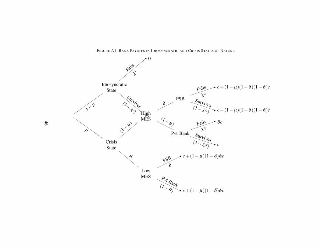
Consider the following simple model (see Figure A1). Nature selects either
of two states, the idiosyncratic state or the crisis state. The idiosyncratic states
occurs with a probability (1− p) and a crisis state occurs with a probability p.
When the idiosyncratic state occurs either of two things can happen –either the
bank fails with a probability λ i in which case it gets a payoff of 0 or it survives
with a probability (1−λ i) in which case it gets a payoff of c. c can be thought
of as the cashflows of the bank or the franchise value of the bank. In case of an
idiosyncratic shock and subsequent bank failure, there is no difference between
a public sector or a private sector bank. Both types of banks get a value of zero
in case of a failure. The assumption is that government guarantees do not kick
in the idiosyncratic state and hence there is no difference between a public and
private sector banks.
Now consider the case when there is an aggregate shock. A mass (1 − µ)
of banks have high MES and the remaining µ banks have low MES. Let this41
economy have a proportion of θ PSBs and (1 − θ) private sector banks. If
a system-wide shock hits the economy, then high MES banks will fail with a
high probability whereas low MES banks will fail with a low probability. For
simplicity, let us assume that low MES banks do not fail whereas high MES
banks have some non-zero probability of failing . Let λ q be the probability that
a high MES bank fails when there is an aggregate shock and (1− λ q) be the
probability that it survives. Now if a high MES bank survives then it gets the
full amount c of cashflows. If it fails, however, private and public sector banks
get different amounts. The crucial assumption here is that PSBs are government
guaranteed.
Let us first consider the simple case when no banks fail. Note, our simplifying
assumption says that low MES banks do not fail. We need to only consider the
high MES banks. With probability (1−λ q) no high MES bank fails. In this case,
all banks receive a payoff of c similar to the idiosyncratic case.
Now consider the case when some high MES banks fail which happens with
a probability (λ q). However, the presence of government guarantees for PSBs
implies that private sector banks are more adversely affected compared to PSBs.
A failing private sector bank which has no government guarantees receives a
lower cashflow of δc, where δ < 1. One can also think of c as the demand for
bank services. When a high MES private sector bank fails (which happens with
probability λ q), then there is a (1− δ )c of gap in demand for bank services.
This demand in bank services is filled in by the surviving banks, that is, between
the public sector (both high and low MES) banks and the remaining low MES
private sector banks. We now introduce another parameter φ which controls the
distribution of this excess demand between high MES PSBs and low MES banks
(both PSBs and private sector banks).
42
Given the above setup we can calculate the franchise values for the banks in
each state. The franchise value for a High MES Public Sector Bank (PSB) is
given by c+(1− µ)(1− δ )(1− φ)c. The value for a High MES Private bank
that fails is δc and High MES Private bank that survives is c. The franchise
value for a Low MES bank is given by c+(1− µ)(1− δ )φc. This is shown in
Figure A1.
We now look at some testable implications from this simple setup. Specifically,
we want to relate how the ex ante bank franchise value changes as the probability
of an aggregate crisis increases. Additionally, we want to relate franchise value
of banks to their vulnerability as measured by MES.
Let V Pvt and V PSB represent the franchise value of the private sector banks and
PSBs respectively. Let ∆V PSB represent the difference in franchise value between
This eventually resulted in a money market and credit squeeze which spilled
over into the real economy.20 The global slowdown also resulted in a slump in
demand for exports. This impact was felt economy-wide and Indian GDP fell
from 9 percent in 2007 to nearly 6.1 percent in 2008. Eventually, the government
of India, fearing an even rapid deterioration of the economy, announced wide-
ranging stimulus packages towards the end of 2008 that appeared to temporarily
restore the economy back to its pre-2008 growth.
20Duvvuri Subbarao,“Impact of the Global Financial Crisis on India Collateral Damage andResponse”, Feb 18, 2009.http:www.rbi.org.inscriptsBS SpeechesView.aspx?Id=410
49
Before 2008, private banks such as ICICI Bank, Karnataka Bank, Lakshmi
Vilas Bank and Kotak Mahindra topped the list of banks with highest NPAs. The
scenario changed drastically in the aftermath of the crisis. After 2008, the gross
non-performing assets (NPAs) of the PSBs grew almost six times to to Rs 3,416
billion in March 2016 and PSBs such as State Bank of India (SBI) and Indian
Overseas Bank topped the list of banks with highest NPAs.
50
D. Robustness Checks
This section reports the results of some robustness checks on our analysis.
A. Stability of MES Ranks over Time
A measure of bank vulnerability that varies substantially over time could make
it difficult to determine whether banks which were more vulnerable in 2006
remained among the more vulnerable banks in 2007, from 2007 to 2008, and
so on. Figure D2 in the appendix plots the MES rankings from January 2006
-December 2006 against the MES ranks from January 2007 - December 2007
confirming that MES rankings in 2006 were reflective of which banks would be
systemically important in 2007.
B. Placebo Tests outside of the Crisis
Table D5 (columns 1–3), Panel A in the appendix show the regressions for
public and private sector banks with the dependent variable as the placebo
“crisis” period returns corresponding to 2005, 2006 and 2007. The corresponding
regressor variables are the “pre-crisis” period MES for the years 2004, 2005
and 2006. The interaction term with MES is insignificant for all periods.
Thus, annual returns in the non-crisis periods, namely 2005, 2006 and 2007
are not explained by the prior year MES. Only, in times of a crisis, the
government guarantees start to matter and affect private and public bank returns
differently. Panel B shows similar regressions results for public and private
sector banks with the dependent variable as the placebo “crisis” period deposit
growth corresponding to 2005, 2006 and 2007. The corresponding regressor
variables are the “pre-crisis” period MES for the years 2004, 2005 and 2006.
The interaction term with MES for PSBs is insignificant for all periods, though51
negative and significant for private sector banks. Thus, annual deposit growth
in the non-crisis periods, namely 2005, 2006 and 2007 are not explained by the
prior year MES.
C. Alternative Measures of Risk
Table D3 in the appendix repeats tests of our basic hypothesis using other
common measures of risk. The regression of event returns against beta and
volatility give results similar to Section II. Regression with volatility as the
risk measure yields a positive and insignificant term for PSBs and a negative
and significant term for private sector banks similar to our results in Table 1.
Regression coefficients using beta and for a two factor model containing the
domestic market return and the global market return are also shown in columns
2 and 3 respectively. The interaction term with beta for dependent variable event
return is positive and significant for public sector banks in both column 2 and
column 3. One might reason that private sector banks had lower returns because
of higher exposure to the global markets. In order to test this hypothesis, we
estimate the coefficients of beta and global beta to estimate the exposure to global
markets. The beta coefficient measures sensitivity to the NSE stock market index.
The global beta coefficient measures sensitivity to the MSCI World market index.
The coefficient for global beta is insignificant and negative for both public and
private sector banks. Thus, exposure to the global markets cannot explain the
difference in behavior of public sector versus private sector banks. Regression of
risk measures against deposit growth show similar results (columns 6–10).
Table D4 uses a modified version of the MES and repeats the analysis. Ex-ante
bank vulnerability is measured by modified MES. Modified MES is the marginal
expected shortfall of a stock given that the banking index return is below its 5th -52
percentile during the period 1st January, 2007 to 31st December, 2007. Banking
sector return is for the pre-crisis period from January 2007 to December 2007 and
is calculated using a price-weighted index of all banks in the analysis leaving out
the bank under consideration. We see that our baseline results remain using the
modified MES.
D. Leverage and Pre-Crises Returns
Leverage is measured as the ratio of the quasi-market value of assets to the
market equity. It is an important predictor of returns during the crisis as shown in
Acharya et al. (Forthcoming). However, we see from Table D3 that leverage was
not a strong predictor of returns for banks in our analysis. Since leverage data
may not be entirely reliable due infrequent and limited balance-sheet reporting
by banks, we proxy for it with pre-crisis returns. The interaction term for crisis
return is significant and negative for private sector banks indicating that more
highly levered banks (due to greater loss of equity capitalization) performed
worse during the crisis.
53
TABLE D1—BANK DATA DURING 2007–2009
Panel A: Public Sector Banks
Bank Name MES Pre-crisis Returns Crisis Returns Deposit Growth Loan GrowthAllahabad Bank 0.04 0.03 -0.66 0.17 0.17Andhra Bank 0.04 0.02 -0.59 0.18 0.25Bank of Baroda 0.04 0.09 -0.55 0.24 0.29Bank of India 0.06 0.08 -0.41 0.23 0.23Bank of Maharashtra 0.03 0.10 -0.75 0.22 0.16Canara Bank 0.05 0.02 -0.53 0.19 0.25Central Bank of India 0.01 0.02 -0.76 0.17 0.16Corporation Bank 0.04 0.02 -0.63 0.29 0.21Dena Bank 0.06 0.13 -0.66 0.24 0.23Indian Bank 0.04 0.10 -0.54 0.17 0.25Indian Overseas Bank 0.04 0.06 -0.76 0.17 0.21Oriental Bank of Commerce 0.05 0.02 -0.63 0.23 0.23Punjab National Bank 0.05 0.03 -0.48 0.23 0.26State Bank of Bikaner and Jaipur 0.01 0.10 -0.97 0.14 0.17State Bank of India 0.05 0.09 -0.54 0.32 0.26State Bank of Mysore 0.03 0.10 -0.71 0.18 0.20State Bank of Travancore 0.01 0.08 -0.70 0.17 0.15Syndicate Bank 0.05 0.05 -0.57 0.20 0.24UCO Bank 0.05 0.18 -0.64 0.23 0.22Union Bank of India 0.06 0.07 -0.42 0.29 0.26Vijaya Bank 0.05 0.08 -0.73 0.13 0.11
54
Panel B: Private Sector Banks
Bank Name MES Pre-crisis Returns Crisis Returns Deposit Growth Loan GrowthAxis Bank 0.04 0.11 -0.63 0.29 0.31Bank of Rajasthan 0.04 0.35 -0.75 0.09 0.05City Union Bank 0.04 0.15 -0.71 0.24 0.22Development Credit Bank 0.05 0.14 -0.89 -0.27 -0.22Dhanalakshmi Bank 0.04 0.10 -0.49 0.32 0.42Federal Bank 0.03 0.10 -0.61 0.22 0.17HDFC Bank 0.03 0.06 -0.51 0.35 0.44ICICI Bank 0.05 0.04 -0.73 -0.11 -0.03IndusInd Bank 0.06 0.17 -0.76 0.15 0.21ING Vysya Bank 0.03 0.10 -0.62 0.20 0.13Jammu & Kashmir Bank 0.02 0.04 -0.72 0.14 0.10Karnataka Bank 0.03 0.05 -0.73 0.18 0.09Karur Vysya Bank 0.03 0.06 -0.54 0.19 0.10Kotak Mahindra Bank 0.05 0.22 -0.81 -0.05 0.07Lakshmi Vilas Bank 0.03 0.08 -0.65 0.27 0.31South Indian Bank 0.04 0.15 -0.76 0.18 0.13Yes Bank 0.04 0.08 -0.80 0.20 0.27
Note: This table contains the list of 38 Indian banks used in our analysis. Panel A contains the public sector banks and panel B contains theprivate sector banks. MES, Pre-Crisis Returns, Crisis Returns, Deposit Growth and Loan Growth are shown. MES (shown in percentage) isthe marginal expected shortfall of a stock given that the market return is below its 5th-percentile during the period 1st January, 2007 to 31st
December, 2007. Market return is based on the S&P CNX NIFTY for the pre-crisis period from January 2007 to December 2007. Beta is basedon the S&P CNX NIFTY index as the market return. Pre− crisis return is the stock return for the period January 2007 to December 2007.Crisis return is the stock return for the period January 2008 to February 2009. Deposit growth for the crisis period is calculated for the periodfrom 31st March, 2008 to 31st March, 2009. Loan growth for the crisis period is calculated for the period from 31st March, 2008 to 31st March,2009. The 38 banks for which both MES data and RBI deposit growth estimates are available were used in this analysis.
55
TABLE D2—SUMMARY STATISTICS
(1)
Private Sector Banks Public Sector Banks TotalMES 0.0383 0.0414 0.0400
N 17 21 38Note: This table contains the summary statistics for MES, Beta, Volatility, GlobalBeta,LogAssets, Leverage, Pre −Crisis Return, Crisis Return, Deposit Growth, 2 year DepositGrowth, and Advances Growth for the 38 banks used in our analysis. Ex-ante bank vulnerabilityis measured by MES. MES is the marginal expected shortfall of a stock given that the marketreturn is below its 5th- percentile during the period 1st January, 2007 to 31st December, 2007.Market return is based on the S&P CNX NIFTY for the pre-crisis period from 1st January, 2007to 31st December, 2007. Volatility is the annualized daily volatility in the pre-crisis period fromJanuary 2007 to December 2007. Beta is based on the S&P CNX NIFTY index as the marketreturn. Global Beta is based in the MSCI World Index returns. Log Asset is the natural logarithmof the book value of asset value measured as of March 31st, 2008. Leverage ratio measured asof March 31, 2008 is the ratio of market equity to the quasi–market value of assets measuredas (book value of assets - book value of equity + market value of equity). Pre-crisis return isthe stock return for the period January 2007 to December 2007. Crisis return is the stock returnduring the crisis calculated from 1st January, 2008 to 24th February, 2009. Deposit Growth is thegrowth in deposits for the period March 2008 to March 2009. Advances Growth is the growth inadvances (loans) for the period March 2008 to March 2009. The 38 banks for which data for allvariables is available were used in the overall analysis.
56
TABLE D3—CRISIS RETURN AND DEPOSIT GROWTH VERSUS MES, BETA, VOLATILITY, LEVERAGE AND PRE-CRISIS RETURNS
Number of Observations 38 38 38 38 38 38 38 38 38 38Adj R-squared 0.972 0.980 0.980 0.965 0.967 0.741 0.747 0.735 0.714 0.726Standard errors in parentheses∗ p < 0.10, ∗∗ p < 0.05, ∗∗∗ p < 0.01
Note: Results are for crisis returns and deposit growth against alternative measures of risk and leverage. Crisis return and deposit growth as calculatedpreviously. Beta and global beta is based on the S&P CNX NIFTY index and MSCI World Index returns respectively. Annualized daily volatility is for January2007–December 2007. Leverage (as of March 31, 2008) is ratio of the quasi- market value of assets (book value of assets - book value of equity + market valueof equity) to the market equity.
57
TABLE D4—CRISIS RETURN AND DEPOSIT GROWTH VERSUS MODIFIED AGGREGATE RISK
MEASURE
(1) (2)Event Return Deposit Growth
PSB -0.88∗∗∗ 0.13∗∗∗(0.11) (0.03)
Pvt -0.65∗∗∗ 0.22∗∗∗(0.07) (0.08)
Modified MES*PSB 7.48∗∗ 2.52∗∗∗(3.11) (0.88)
Modified MES*Pvt -1.73 -2.85(2.44) (3.14)
N 38 38Adj R-squared 0.973 0.730Standard errors in parentheses∗ p < 0.10, ∗∗ p < 0.05, ∗∗∗ p < 0.01
Note: Results for crisis returns and deposit growth against another alternative measures of risk is shown.Crisis return is the stock return during the crisis calculated from 1st January, 2008 to 24th February, 2009.Deposit growth is measured from 31st March, 2008 to 31st March, 2009. Ex-ante bank vulnerability ismeasured by modified MES. Modified MES is the marginal expected shortfall of a stock given that thebanking return is below its 5th - percentile during the period 1st January, 2007 to 31st December, 2007.Market return is based on the S&P CNX NIFTY for the pre-crisis period from January 2007 to December2007. The banking index is calculated using a price-weighted index of all banks in the analysis leaving outthe bank under consideration. The 38 banks for which data for all variables is available were used in thisanalysis. Standard errors are heteroskedasticity robust and shown in parenthesis.
58
TABLE D5—PLACEBO TESTS
Panel A: Event Return(1) (2) (3)
2005 versus 2004 2006 versus 2005 2007 versus 2006PSB 0.174 -0.028 0.695∗∗∗
(0.136) (0.137) (0.123)
Pvt 0.378 0.464∗∗ 0.531∗∗∗(0.256) (0.172) (0.124)
MES * PSB -2.276 3.595 -3.468(2.066) (5.679) (2.507)
MES * Pvt -6.349 -7.560 5.050(4.523) (6.838) (3.340)
Number of Observations 37 37 37Adj R-squared 0.029 0.369 0.837
Panel B: Deposit Growth(1) (2) (3)
2005 versus 2004 2006 versus 2005 2007 versus 2006PSB 0.007 0.110 0.563
MES * PSB 2.069 1.479 -5.090(1.695) (5.058) (7.167)
MES * Pvt -6.810∗∗ -2.941 -1.890∗∗(2.607) (2.238) (0.923)
Number of Observations 36 37 37Adj R-squared 0.592 0.081 0.307Standard errors in parentheses∗ p < 0.10, ∗∗ p < 0.05, ∗∗∗ p < 0.01
Note: Panel A shows the regression results of the placebo tests for placebo crisis returns versusMES. Panel B shows the regression results of the placebo tests for placebo deposit growthversus MES. MES is the marginal expected shortfall of a stock given that the market return isbelow its 5th - percentile during the period 1st January to 31st December in the placebo pre-crisisperiod. Market return is based on the S&P CNX NIFTY for the pre-crisis period from Januaryto December of the placebo pre-crisis period. Placebo crises returns are calculated from 1st
January to 31st December of the crises period. For example, 2005 versus 2004 regression resultsare carried out using crisis period returns from January 1st to December 31st, 2005 against pre-crisis period returns calculated from January 1st to December 31st, 2004. Returns are similarlycalculated for 2006 versus 2005 and 2007 versus 2006. Placebo deposit growth is calculatedfrom annually from March 31st of each year. For example, for the 2005 versus 2004 regressionis carried out using placebo crisis period deposit growth from March 1st,2005 to March 31st,2006 against placebo pre-crisis period MES calculated from January 1st to December 31st, 2004.Deposit growth is similarly calculated for 2006 versus 2005 and 2007 versus 2006. We use the 38publicly listed banks for which data is available from RBI. Standard errors are heteroskedasticityrobust and shown in parenthesis.
59
TABLE D6—SUMMARY STATISTICS FOR DEPOSITS GROWTH BY TYPE
Interbank term Deposits 0.123 0.425 0.290(0.612) (0.931) (0.808)
Corporate/Retail Term Deposits 0.207 0.283 0.249(0.255) (0.0951) (0.186)
N 17 21 38Standard deviation in parentheses
Note: This table shows the descriptive statistics for growth of different types of deposits. Depositgrowth for the crisis period is calculated from data provided by Reserve Bank of India (RBI) forthe period from 31st March, 2008 to 31st March, 2009. Deposits are classified into (A) demanddeposits, (B) term deposits and (C) savings. Deposits can also be classified based on location intodeposits belonging to branches within India. Demand and term deposits are further classified intocorporate/retail deposits and interbank deposits. The 38 banks for which data for all variables isavailable were used in this analysis.
60
TABLE D7—SUMMARY STATISTICS FOR GROWTH IN LENDING AND LENDING RATES
Private Sector Banks Public Sector Banks TotalOverall 0.162 0.216 0.192
(0.163) (0.0471) (0.116)
Priority Sector and public sector firms 0.137 0.172 0.156(0.162) (0.0961) (0.129)
Note: This table shows the descriptive statistics for growth in loans (advances) by type andlending rates. Overall growth in loans (advances) for the crisis period is calculated for the periodfrom 31st March, 2008 to 31st March, 2009. Panel A shows growth in loans in each category,namely, growth in lending to the priority and public sector firms and growth in lending to banks.All other categories are classified under other. Lending rates are calculated as follows. Q1 2008is the average prime lending rate for the period from January 2008 to March 2008, Q2 2008 isfrom April 2008 to June 2008, Q3 2008 is from July 2008 to September 2008, Q4 2008 is fromOctober 2008 to December 2008 and Q1 2009 is from January 2009 to March 2009. The 38banks for which data for all variables is available were used in this analysis.
61
6080
100
120
140
160
Inde
x w
ith b
ase
= 10
0 in
Jan
200
7
01jan
2007
01jul
2007
01jan
2008
01jul
2008
01jan
2009
S&P NIFTY Index BSE Index
BSE and S&P NIFTY Index
5010
015
020
025
0
Inde
x w
ith b
ase
= 10
0 in
200
7
01jan
2007
01jul
2007
01jan
2008
01jul
2008
01jan
2009
Private Sector Banks PSBs
Value Weighted Index
FIGURE D1. STOCK INDEX PERFORMANCE
Note: The left panel shows stock index performance for the period starting January 2007 to January 2009. Two indices, S&P NIFTY and BSESENSEX, are represented. The S&P CNX NIFTY is a free float market capitalization index on the National Stock Exchange and consists of50 companies. Bombay Stock Exchange Sensitive Index (BSE Sensex or Sensex) is a value-weighted index composed of 30 stocks. The rightpanel shows the indexed value weighted returns for the private (public) sector banks used in our analysis weighted by their market capitalization.A base value of 100 as of January 2, 2007 is used for all plots. The beginning of the crisis January 2008, is indicated with a vertical dashed line.
62
FIGURE D2. MES RANK FOR JAN ’07–DEC ’07 VERSUS MES RANK FOR JAN ’06–DEC ’06
IDBIIDB
DENAUNION
BOICANARA
OBCVIJAYA
PNBDCB
SYNDICATEUCO
SBIICICI
KMBBOB
ALLHBDYBL
BORINDIAN
IOBSOUTHIND
DBLANDHRA
CUNAXIS
CORPFED
HDFCKRNTKA
ING VSBM
KARURBOMAHRSHTRA
LVBJ&K
SBJCBI
SBT
010
2030
40M
ES
ran
k 20
07
0 10 20 30 40MES rank 2006
Note: The graph above shows the scatter plot of the MES Rank computed during the period 1st January, 2007 to 31st December, 2007 versusthe MES Rank computed during the period from 1st January, 2006 to 31st December, 2006. MES for a period is the marginal expected shortfallof a stock given that the market return is below its 5th - percentile during the same period. Market return is based on the S&P CNX NIFTY.”MES Rank” ranks banks in descending order of MES values (assigns rank 1 to the bank with the largest MES). The 38 banks for which datawas available for both periods were used in the analysis.
63
0.1
.2.3
Foreign Private Public
All Deposit (YoY)
07-08 08-09
0.1
.2.3
.4
Foreign Private Public
Demand Deposit (YoY)
07-08 08-09
0.1
.2.3
.4
Foreign Private Public
Savings Deposits (YoY)
07-08 08-09
0.1
.2.3
.4
Foreign Private Public
Term Deposit (YoY)
07-08 08-09
0.1
.2.3
Foreign Private Public
Credit (YoY)
07-08 08-09
.13
.09
.06
.02.02
.07
.03.03
.1.1
0.02
.01
.06
0
.05
.08
.12
0.0
5.1
.15
07 Q
107
Q2
07 Q
307
Q4
08 Q
108
Q2
08 Q
308
Q4
09 Q
1
All Deposit (QoQ)
Private PSB
Gro
wth
Rate
FIGURE D3. DEPOSIT AND CREDIT GROWTH
Note: The figures above show the bank group-wise growth in deposits and credit for foreign banks, public sector banks and private sector banksin India. Deposits are classified into demand deposits, term deposits and savings deposits. Growth rates are year-on-year from March 2008 toMarch 2009 for all graphs except the bottom-rightmost panel which shows quarter-on-quarter deposits growth from Q1 2007 to Q1 2009. Datais from the Reserve Bank of India (RBI).
64
AXIS
BOR
CUN
DCBDBLFED
HDFC
ICICI
IDB
ING V
KRNTKAKARUR
KMBLVB
SOUTHIND
YBL
J&K-.005
0.0
05.0
1
.02 .03 .04 .05 .06
PrivateSBI
SBJ SBMSBT ALLHBDANDHRA
BOB BOI
BOMAHRSHTRACANARACBI
CORP
DENAINDIAN
IOB
OBCPNB
SYNDICATE
UCOUNION
VIJAYA
0.0
01.0
02.0
03.0
04
.01 .02 .03 .04 .05 .06
PSB
Mar
ch 0
8-Ju
ne 0
8
AXIS
BOR
CUN DCBDBL
FED
HDFC
ICICI
IDB
ING V
KRNTKAKARUR KMB
LVB
SOUTHIND
YBL
J&K
0.0
05.0
1.0
15
.02 .03 .04 .05 .06
Private
SBI
SBJ
SBM
SBT
ALLHBD
ANDHRABOB
BOI
BOMAHRSHTRA
CANARA
CBICORP
DENA
INDIANIOB
OBC
PNBSYNDICATE
UCO
UNION
VIJAYA
0.0
05.0
1.0
15
.01 .02 .03 .04 .05 .06
PSB
June
08-
Sept
08
AXISBOR
CUN
DCB
DBLFEDHDFC
ICICI
IDB
ING V
KRNTKAKARUR
KMB
LVB
SOUTHIND
YBL
J&K
-.01
-.005
0.0
05.0
1.0
15
.02 .03 .04 .05 .06
Private
SBI
SBJ
SBM
SBT
ALLHBD
ANDHRA
BOB
BOIBOMAHRSHTRA
CANARACBI
CORP
DENAINDIAN
IOB
OBC
PNBSYNDICATE
UCO
UNION
VIJAYA
-.01
-.005
0.0
05
.01 .02 .03 .04 .05 .06
PSB
Sept
08-
Dec
08
AXIS
BORCUNDCB
DBL
FED
HDFC
ICICIIDB
ING VKRNTKA
KARUR
KMB
LVB
SOUTHIND
YBL
J&K
-.015
-.01
-.005
.02 .03 .04 .05 .06
Private
SBI
SBJ
SBM
SBT
ALLHBD
ANDHRA
BOB
BOI
BOMAHRSHTRA
CANARA
CBI
CORP
DENA
INDIAN
IOB
OBCPNB
SYNDICATE
UCO
UNION
VIJAYA
-.015
-.01
-.005
.01 .02 .03 .04 .05 .06
PSB
Dec
08-
Mar
ch 0
9
MES
FIGURE D4. DEPOSIT RATES VERSUS MES FOR SHORT TERM MATURITIES
Note: The above graphs change in deposit rates for short maturity (< 3 year) term deposits from March 2008 to June 2008, from June 2008to September 2008, from September 2008 to December 2008 and from December 2008 to March 2009 against the ex-ante measure of bankvulnerability, MES. Average deposit rate for each bank is calculated as average of minimum and maximum deposit rate provided by RBI. MESis calculated as in Table 1. The 38 banks for which data for all variables is available were used in this analysis.
65
Panel A: NPAAdvances
0.0
5.1
.15
.2N
PA/A
dvan
ces
2007 2008 2009 2010 2011 2012 2013 2014 2015
PSB Private
Panel B: Restructured LoansAdvances
0.0
2.0
4.0
6.0
8.1
Res
truct
ured
Loa
ns/A
dvan
ces
2007 2008 2009 2010 2011 2012 2013 2014 2015
PSB Private
FIGURE D5. NPA AND RESTRUCTURED LOANS FROM 2007–2015
Note: The figures show average NPA to advances (Panel A) and restructured loans to advances(Panel B) for the period March 2007 to March 2015 separately for public and private sector banks.NPA (gross NPA), advances and restructured loans data is publicly available for each fiscal yearfrom the Reserve Bank of India (RBI). The 38 banks for which data is available were used in thisanalysis.