Government, Primary Healthcare, and Standard of Living: Evidence from Costa Rica Luis Diego Granera Vega * October 18, 2021 Abstract I study whether a coordinated effort by a government to increase access to healthcare through increased expenditure would bring about higher incomes at the household level. Using data from the major healthcare reform that Costa Rica underwent in 1994, which greatly increased access to primary healthcare, I explore the effects of get- ting local clinics in their district, as a result of the reform, on household and personal income. Based on theoretical work by Strauss and Thomas (1998) and a seminal paper by Grossman (1972), my main hypothesis is that, by producing healthier individuals, having increased access to healthcare spurs individuals to pursue better-paying jobs, thereby increasing their income. I proceed by difference-in-difference, as well as by an event study specification, both of which point to a positive average impact of around 4% of getting a clinic on income. Keywords: National Government Health Expenditure, Health, Development, Eco- nomic Growth, Fiscal Policy JEL Codes: H51,I150, O23 * PhD student, Department of Economics, University of Washington, Seattle.
Transcript
Government, Primary Healthcare, and Standard of
Living: Evidence from Costa Rica
Luis Diego Granera Vega∗
October 18, 2021
Abstract
I study whether a coordinated effort by a government to increase access to healthcare
through increased expenditure would bring about higher incomes at the household
level. Using data from the major healthcare reform that Costa Rica underwent in
1994, which greatly increased access to primary healthcare, I explore the effects of get-
ting local clinics in their district, as a result of the reform, on household and personal
income. Based on theoretical work by Strauss and Thomas (1998) and a seminal paper
by Grossman (1972), my main hypothesis is that, by producing healthier individuals,
having increased access to healthcare spurs individuals to pursue better-paying jobs,
thereby increasing their income. I proceed by difference-in-difference, as well as by an
event study specification, both of which point to a positive average impact of around
4% of getting a clinic on income.
Keywords: National Government Health Expenditure, Health, Development, Eco-
nomic Growth, Fiscal Policy
JEL Codes: H51,I150, O23
∗PhD student, Department of Economics, University of Washington, Seattle.
1 Introduction
Can a government expansion of healthcare access cause changes in household income? Using
data from Costa Rica, my analysis points to an increase in household income of around 4% as
a result of furthering access to primary healthcare. This comes to add to the literature that
has studied the mechanisms and direction of the relationship between healthcare spending,
health, and economic development.
At the macroeconomic level, there is evidence of a two-sided relationship between eco-
nomic growth and healthcare spending through improved health and life expectancy. Using
data from 48 African countries, Some, Pasali, and Kaboine (2019) [30] established that
healthcare spending increases life expectancy and promotes economic growth. In turn, with
data from rich, middle, and low-income countries, Acemoglu and Johnson (2007) [2] found
that increased life expectancy promotes economic growth. Moreover, from a panel of ten
countries, Bloom, Canning, and Sevilla (2004) [9] concluded that health of the workforce
stimulates economic growth. Furthermore, Alhowaish (2014) [3] showed a relationship of
Granger causality of economic growth on healthcare spending.
At the microeconomic level, the focus of my analysis, there is evidence of a relationship
between household income and individual health. Fichera (2015) [14] observed that increases
in income reduce illness, while Contoyannis and Dooley (2010) [11] noted that socioeconomic
status as children affects health as young adults. Meanwhile, Case, Lubtsky and Paxson
(2002) [10] found that health in children is positively correlated with household income.
Additionally, Strauss and Thomas (1998) [31] laid theoretical groundwork to a causal positive
impact of health on wages, while Thomas and Frankenberg (2002), in their Bulletin of the
World Health Organization article [32] shared empirical results suggesting nutrition as a link
between healthier workers and higher wages.
Adding health insurance into the discussion, from a panel of 100 countries, Moreno-Serra
and Smith (2012) [23] established that broader health insurance coverage leads to better
access to healthcare and improved health, particularly for lower income groups. And even
1
whole populations can benefit economically from healthcare, as McDermott, Cornia, and
Parsons (1991) concluded that getting a hospital in a rural community makes “significant
economic contributions to the community they serve” [21].
We can therefore observe that, in one direction, higher income results in better health. I
want to more deeply understand how the relationship holds in the opposite direction. We do
know that adequate health insurance results in better care, which promotes improved health
[23], which translates into higher wages at the micro level, with theory [31] and weaker
empirical results [32], though so far this chain of events has not been studied as a whole.
All of this made me wonder if this process could be explained by a government interven-
tion. In particular, I wanted to know if a coordinated effort by a government to increase
access to healthcare through increased expenditure, using data from Costa Rica, would bring
about higher incomes at the household level. This would come to strengthen Thomas and
Frankenberg’s conclusions [32] through a different channel, provide further empirical evidence
for Strauss and Thomas’s theoretical model, and advance the understanding on government
interventions in the healthcare sector in the context of universal health insurance.
There is already some evidence connecting access to healthcare to individuals’ health
level. For instance, it is known that bigger distances to healthcare clinics are correlated
with worse health outcomes. Croke et al (2020) [12] studied a reform in Ethiopia that built
almost 3,000 government clinics and its impact on maternal utilization and birth outcomes.
They found increased prenatal care of 0.38 visits and a 7.2% increase in deliveries in-place
per every new clinic opened within 5km. Additionally, focusing on the construction of
maternity facilities in Malawi, Quattrochi et al (2020) [27] established that bigger distances
to the clinics are related to lower healthcare utilization and higher under-five mortality. And
similarly, using data from India, Kumar, Dansereau, and Murray (2014) [19] observed that
women living farther from health facilities are less likely to give birth there. Each extra
kilometer to the nearest clinic is associated with a 4.4% decrease in the probability of giving
birth in-facility.
2
Finally, there has also been important previous work on whether health interventions can
cause changes in income, just as educational interventions like building schools in Indonesia
did for those in treatment [13]. In their ’Worms at Work’ paper (2016) [5], Baird, Hicks,
Kremer, and Miguel studied the long-term effects of a deworming intervention in Kenya (cf.
Kremer and Miguel (2004) [22]). They found that men who were exposed to the treatment
as children worked 17 % more hours and that overall, incomes were on average 26.9% higher.
Moreover, they concluded that the financial returns to deworming of 32% more than make
up for the cost of the program, underscoring the economic potential interventions like these
have.
With near-universal health insurance, Costa Rica provides an ideal case study to test the
hypotheses of this project, as it allows me to skip the step of changing the health insurance
status quo and start the analysis at changes in healthcare availability. A place where access
to healthcare is determined by physical availability [20], not its affordability, Costa Rica
underwent a healthcare reform in the mid-1990s that greatly expanded access to primary
healthcare. Did this have an impact on household income? My analysis concludes an increase
in household income of around 4% as a result of furthering access to primary healthcare.
2 Background
Before 1994, the management of the Costa Rican healthcare sector was shared between the
Ministry of Health and the Social Security Administration [34]. The former was established
in 1922 and, from its inception, its functions were focused on prevention and education, along
with the provision of some basic medical care. The latter came to be in 1941 and it was
designed to provide healthcare and pensions to all workers, minors, pregnant women, and the
poor, funded by a combination payroll taxes, employer taxes, and government contributions.
For over fifty years they would share this partial overlap of functions.
The 1980s brought with the economic downturn both a steep increase in national debt
3
and deep austerity measures, including cuts to healthcare spending [17]. This resulted in a
decrease in service quality and patient satisfaction. As a response, in 1994 the government
decided to enact a major reform to the healthcare system, switching all preventative, public
health, and medical treatment responsibilities from the Ministry of Health to the Social
Security Administration (CCSS), centralizing both funding and decision-making in order
to improve efficiency. For comparison, achieving a similar level of integration in the United
States would require merging the Centers for Disease Control and Prevention (CDC) with the
Department of Veterans’ Affairs (VA), and the Centers for Medicare and Medicaid Services
[25].
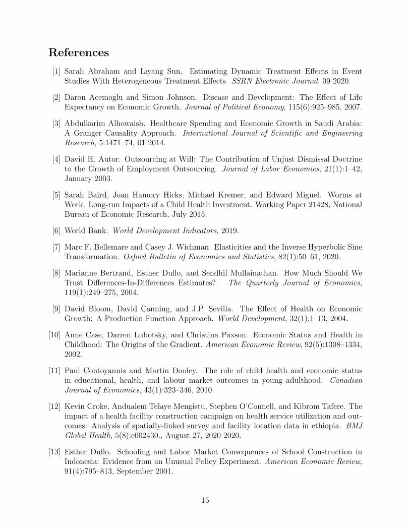
The reform divided the country into 104 areas of 40.000 to 100.000 people each, where
it would establish small clinics responsible for approximately 4.500 people [25] led by teams
comprised of a physician, a nurse, a community health worker, a pharmacist, and a clerk in
charge of detailed health data collection [33]. (The first teams were established at already-
existing clinics, to be followed by building more clinics.) This would provide patients with a
first point of contact to healthcare, combining both preventative, acute, and chronic support,
increasing the depth and breadth of care. These clinics received the name of EBAIS, which
stands for Equipos Basicos de Atencion Integral en Salud, Spanish for “Integrated Teams of
Basic Comprehensive Healthcare”.
As a result of this reform, and despite being a middle-income country, as defined by the
World Bank [6], Costa Rica now exhibits improved health outcomes while spending less than
most of the world [25] both per capita and as a proportion of real gross domestic product:
Costa Rica spends only about $970 per person per year, compared to $1, 061 in the rest
of the world (measured in US $ of 2014), and 9.3% of GDP, compared to 9.9%. Moreover,
maternal, infant, and under-five mortality indicators are low and have decreased steadily over
the last quarter century, as established in his seminal papers on the Costa Rican healthcare
reform by Dr Luis Rosero-Bixby (2004) [28], [29]. Also, life expectancy in Costa Rica is now
nearly five years higher than the rest of Latin America, and almost eight years more than
4
the world average. In fact, in the Western Hemisphere, only Chile and Canada have a higher
life expectancy [24]. This gives Costa Rica the unlikely honor of having become a public
health “positive deviant” [25].
The main policy implication of the reform was that the proportion of the national popu-
lation with access to primary care (that is, within 4 km of their home [29]) went from 25% to
93% in the first twelve years alone. In 2014, the EBAIS clinics provided three-quarters of all
medical consultations and covered the medical needs of 80% of all national patients, giving
some much-needed relief to hospitals [25]. It was learning about this increase in access that
piqued my interest, making me wonder whether, in addition to public health improvements,
any increases in household standard of living could be attributed to the reform.
3 Data
My main source of data is the Encuesta de Hogares de Propositos Multiples (EHPM), or
“Multiple Purpose Household Survey”, an annual, nationally-representative survey of Costa
Rican households given by the Costa Rican Statistics and Censuses Institute (INEC ) between
1987 and 2008. This provides me with a twenty-two-year pooled cross-section of household
data of 30, 000 to 50, 000 observations per year that includes their district, number of peo-
ple per household, age, education, personal and household income, as well as marital and
insurance status of each member, among others. Moreover, in order to ensure that income
variables are comparable across time, I use the Consumer Price Index (CPI), as calculated
by the Costa Rican Central Bank (BCCR), in order to normalize incomes into constant July
2015 colones, the local currency. Additionally, to minimize the effect of outliers I winsorize
the income data, substituting the extreme values beyond the 5th and 95th percentiles with
the values at those percentiles.
In order to determine the districts that benefited from the healthcare reform, I use the
Social Security Administration’s Annual Memories (Memorias Institucionales de la CCSS)
5
to record, year by year, the districts where new EBAIS clinics were built or opened from
1995 to 2008. This serves as a complement to the EBAIS district data from 1995 to 2001
kindly shared with me by Dr Luis Rosero-Bixby.
From among all the 892, 317 observations, I focus on the households located in districts
that did not already have a source of primary healthcare prior to the reform, like a hospital
or clinic. Because the location of those is endogenous, using them would obscure the results
of the analysis of the reform. Table 1 shows summary statistics for the remaining 313, 977
observations: 157, 176 individuals who lived in households whose district either never got
an EBAIS clinic or before it gets one, along with 154, 377 who lived in districts that got
an EBAIS as a result of the reform. These will constitute the comparison and treatment
groups, respectively. In terms of districts, that corresponds to 262 who “always” had a clinic,
59 that “never” did, and 152 that got one “later”, as seen in Figure 1.
Both groups are distributed mostly evenly with regards to number of observations, with
around 155,000, as well as to number of people per household, with around 5. There is some
difference in the proportions of males and females, with the control group having about 5
percentage points more in each, although this could be attributed to the relatively large
number of observations in the treatment group where sex is unknown, 13%. There is also a
difference in age, with people in the treatment group being approximately 40 years old, as
opposed to 30 in the control. Both groups are fairly similar in years of education, with the
treatment group having on average only 0.4 years more. Finally, given an average exchange
rate of 528 Costa Rican colones per US dollar at the time (recall income data is expressed in
colones of July 2015), households in the comparison group had a monthly income of around
$1040, compared to $1,000 in the treatment. Similarly, average personal monthly income in
the comparison group was $205, compared to $211 in the treatment.
6
4 Empirical Strategy
The 1994 Costa Rican healthcare reform has been thoroughly studied from a public health
perspective, as exemplified by the seminal work by Dr Luis Rosero-Bixby [28] [29]. How-
ever, approaching it from an economic point of view would provide a more unique outlook,
establishing the causal link, if any, that the government healthcare reform had on variables
of interest in the Costa Rican economy. In particular, I wish to uncover the treatment effect
of having increased access to primary healthcare on household and personal income, with
the study of education left for my second paper. This comes to add to the literature on the
household effects of building infrastructure, like Duflo’s paper of schools in Indonesia (2001)
[13], and on non-health effects of health reforms, like Miguel and Kremer’s ’Worms at work’
paper (2016) [22].
The rationale behind this pursuit is that having increased access to primary healthcare
would bring about better health outcomes, which in turn translates into higher-quality work-
ers. That is, healthier individuals would make for workers that could aspire to higher-paying
jobs. Given universal health insurance, therefore, it is the availability of healthcare, and not
its affordability, that is the limiting factor in receiving care.
I pursue a difference-in-difference approach, which will constitute the central part of the
empirical analysis. I estimate the effect on both personal and household income Yidt for
household i in district d at year t of Clinicdt, an indicator for a district d having a clinic as a
result of the reform at time t that did not have any source of primary healthcare beforehand,
as well a matrix of controls X, year fixed effects λt, and district fixed effects γd. It should
also be noted that I am only studying districts that did not already have a clinic before
1995, as the placement of those previously-established clinics is endogenous. That way I
can better assess the difference in outcomes as a result of the healthcare reform, despite its
quasi-experimental nature.
7
The equation estimated is
Yidt = αClinicdt +X ′itβ + λt + γd + εidt (1)
where the coefficient of interest is α, the treatment effect on the treated. Also, for all
regressions, heteroskedasticity-robust standard errors are clustered at the district level [8].
I should acknowledge two limitations of this approach: First, that the decision of where
to open the EBAIS clinics was not random, as the government gave priority to lower-income
areas, so making a case for identification will be an important step in the process. And
second, that there is a growing literature about potential pitfalls in the use of difference-
in-difference, as exemplified by the Duflo, Bertrand, and Mulhanaithan (2004) paper [8],
which warns about the potential inconsistency of the resulting standard errors. Moreover,
if using more than two periods’-worth of data, a more recent working paper by Goodman-
Bacon (2019) [15] calls into question the interpretation of the coefficient of interest as an
average treatment effect on the treated, suggesting instead that it is a weighed average of
all two-period difference-in-difference coefficients.
Finally, I am also interested in analyzing the long-term effects, if any, that the healthcare
reform had on income. To that end, I will use an event-study specification, given all the
years’-worth of data available (8 before and 14 after the passing of the reform). My goal
will be to measure how having a clinic in a treated district affected household and personal
income after a varying number of years.
The equation to estimate is
Yidt =α1Clinicdt +X ′itβ + λt + γd
+12∑
t=−21
ηt · Y earsElapseddt + εidt
8
where Y earsElapseddt measures the number of years since a treated district was treated,
normalizing comparison group values to −30.
4.1 Identification strategy
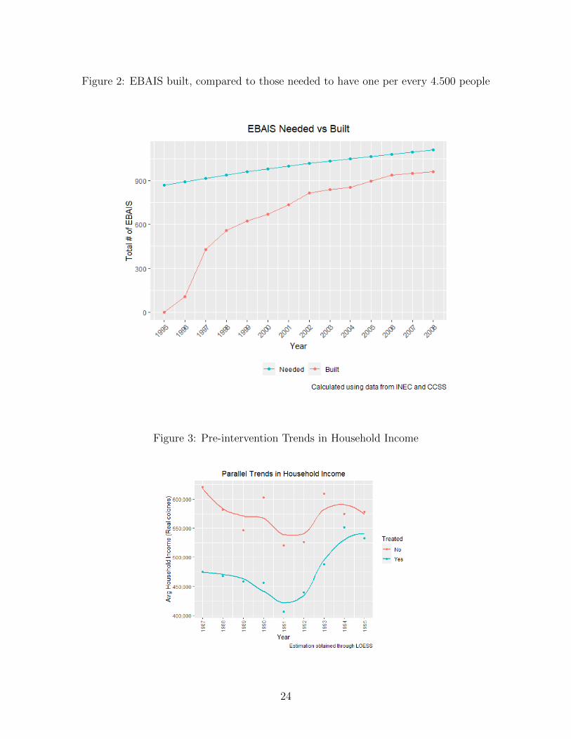
To justify the use of difference-in-difference and an event study [1], I check for parallel trends
in the income variables. A first intuition, providing a necessary but not sufficient condition
for identification, is to look graphically at the trends in income before treatment. I would
want for the slopes to be fairly similar because, if they were not, then income definitely
would not follow parallel trends and I could not use difference-in-difference. Figures 3 and
4 show, using a non-parametric method for household income, as well as linear regression
for personal income, that the trends for the treatment and comparison groups do appear to
be parallel.
The graphs provide only suggestive evidence of parallel trends. Given that treatment was
staggered and there is no single pre- and post-intervention period for the treatment group,
I also follow the methodology suggested by Autor (2003) [4], cited in Pischke (2005) [26], as
a more formal test of the identification assumption. In it, he introduces to the regression
yearly dummies that are interacted with the treatment variable. The desired result is that
the only coefficients to be statistically significant should be those post-intervention.
The model becomes
Yidt = X ′itβ + λt + γd +2008∑1987
βtClinicdtY eart + εidt (2)
where Y eart is a dummy variable corresponding to what year it is.
The test of the difference-in-difference assumption would require that all βt be indistin-
guishable from 0 for the years prior to treatment and that the Clinic ∗ Y ear variables be
jointly insignificant pre-intervention. I would only want and expect for coefficients post-
9
intervention to be positive and statistically significant.
Figure 2 shows the results of this test graphically, with the point estimates along with bars
with their standard errors. Rather surprisingly, because of how the treatment variable was
built, no coefficients are reported prior to the beginning of the reform, 1994. Nevertheless,
this also implies that, vacuously, no pre-intervention coefficient is statistically significant,
so the parallel trends assumption is not violated and we may proceed. Additionally, for
years after the intervention, the estimates for most years are significantly different from 0, as
shown by the 95% confidence intervals. The yearly effects vary between 20, 000 and 40, 000
real colones, or about $38 to $76, with a mean household income of around $1020.
Similarly, Figure 6 shows comparable results in percentages. Again, no results are re-
ported prior to 1994 but most of the post-intervention coefficients are positive and statisti-
cally significant. Yearly estimates compared to the reference year (1994) range from 2% to
8%, again showing significant positive results post-intervention and no significant estimates
pre-intervention.
5 Mechanism
In order to justify the proposed positive causal relationship between an increase in access to
healthcare and increases in income as a result of the 1994 Costa Rican healthcare reform,
I will rely on Strauss and Thomas’ formulation [31] of Michael Grossman’s seminal 1972
model [16] on the link between health and wages.
Here is the intuition behind the results of the model: Increased access to primary health-
care would bring about better health outcomes. This translates into higher-quality/healthier
workers. Healthier individuals would make for workers that could aspire to higher-paying
jobs. Given universal health insurance, therefore, it is the availability of healthcare (Lin-
delow, 2005) [20] and not the ability to pay for it, that is the limiting factor in receiving
care.
10
(For a full account of the theory, see Appendix A.)
Therefore, under this theoretical framework, I would expect for incomes to go up as a
result of the healthcare reform.
6 Results
The difference-in-difference estimation yielded a positive and highly statistically significant
change in income as a result of the healthcare reform. Table 3 shows the effect of getting
an EBAIS on treated districts. Adding district and time fixed effects, as well as controlling
for age, education, insurance type, and marital status, among others, getting an EBAIS led
to an increase of around 17,000 real colones (about $33 of 2015), a positive and statistically
significant increase in average household income as a result of the reform, however modest,
compared to the average monthly income of around $1,022. Without district fixed effects,
the estimate is negative but insignificant, a loss of about 76,000 colones or around $145 in
monthly household income.
Table 4 confirms these results: the treatment effect on the treated is positive (4%), as
hypothesized, and highly statistically significant. This specification also controls for the same
variables, as well as district and time fixed effects. On the other hand, as was the case in
the analysis in levels, without district fixed effects the estimate is negative but insignificant,
a decrease of 14% in household income. This reinforces the importance of the district fixed
effects, since the reform happened at the district level.
Next, Table 5 displays the changes in personal income levels as a result of the healthcare
reform. The two specifications, without and with district fixed effects, respectively, present
either negative or small and positive changes in personal income from getting an EBAIS.
Nevertheless, both changes prove to be statistically insignificant. Without district fixed
effects, the “effect” of the reform was a decrease of around 7,100 real colones or about $13.
Meanwhile, by adding district fixed effects, the negative result disappears, changing sign, to
11
about 535 colones, or around $1.
Correspondingly, Table 6 reports the percent changes in personal income as a result of
the reform, using the inverse hyperbolic sine transformation [7], as some individuals report
zero income (so the logarithm would not be defined). It suggests a statistically insignificant
decrease of 0.2% in personal income as a result of the healthcare reform using time fixed
effects. Without them, the resulting percent change is also a small, negative and insignificant
-0.4%.
This leads me to believe one of two things: first, that combined with the results from
Table 5 discussed above, getting an EBAIS does not appear to have had a positive effect
on individuals; or second, more interestingly, that there might be something special about
families in Costa Rica that make them able to achieve feats impossible or at least impractical
for individuals. Given the collaborative nature of families in Costa Rica, I am led toward
the latter.
Finally, I share the results of the event-study specification. Table 7 reports the estimates
for the effects on households of having been treated with a clinic in their district over several
years, both before and after. As expected, the bulk of the pre-intervention coefficients, small
and positive as well as negative, are insignificant. Although a couple of those coefficients are
indeed significant, which would be indicative of selection, an F-test fails to reject that all
the pre-intervention coefficients are jointly insignificant. In addition, as a result of getting
an EBAIS clinic in their district, I find positive and highly statistically significant increases
in the household income ranging from 19, 000 to 54, 000 colones, or between $36 and $102 of
2015, up to 10 years post-intervention. This corresponds to an increase of between 3% and
7% with respect to the year of treatment. Figure 7 helps visualize these same results.
For personal income, I find statistically significant percent increases up to ten years post-
intervention averaging around 19%. There are four instances of estimates pre-intervention
being statistically significant, but one more time an F-test fails to reject the null that the
pre-intervention coefficients are jointly insignificant. Similarly, looking at results in levels, I
12
find increases ranging from 6, 500 to 12, 000 colones, or $12 to $23 of 2015, and an F-test also
fails to reject the null. That provides evidence for the strength of my event study results on
personal income.
7 Robustness checks
As I explain in the Empirical Strategy section, the identification assumption of difference-in-
difference, parallel trends in income, does seem to hold. First, I find suggestive evidence by
graphing the trends for the treatment and control groups in Tables 3 and 4. Then, I perform
a stronger test by adding time dummies and interacting them with the treatment variable.
Despite the lack of reported coefficients pre-intervention, as seen in Figure 5, this vacuously
indicates a lack of significant coefficients pre-intervention, providing further evidence for
parallel trends.
One aspect I am unable to address stems from a recent paper by Kahn-Lang and Lang
(2020) [18] suggests that the plausibility of parallel trends is greater if the treatment and
control groups start at similar levels, and not just follow similar trends. Nevertheless, given
the quasi-experimental nature of the reform, my treatment and control groups do start at
different levels, which might weaken the argument for parallel trends.
An important decision I made in my empirical analysis was to only focus on those house-
holds that did not already have a source of primary healthcare before the reform. That
reduced the number of observations to about a third, from 892,317 to 311,553, and house-
holds in districts that eventually get a clinic constitute my treatment, while those that never
do are my comparison. Going forward, it would be worthwhile to also repeat the analysis,
but this time with the same treatment group but using the previously discarded observations
as comparison, to check if the results are qualitatively similar.
13
8 Conclusion
Costa Rica underwent a major healthcare reform starting in the 1990s that greatly expanded
access to primary healthcare through its new EBAIS clinics. As a result the reform, now
three-quarters of all medical consultations happen at an EBAIS. The stated goal of the
reform was improving access and quality of care, which would result in better health in-
dicators. Rosero-Bixby [28] showed just that: child mortality went down by 8%, deaths
by transmissible illnesses decreased by 14% and deaths by chronic diseases shrank by 2%,
among others.
This paper discussed the possibility that this reform would also have the unintended
beneficial effect of increasing household or personal incomes. My contention, stemming
from Grossman’s model of healthcare demand [16], was that better access to healthcare
would result in healthier people who could aspire to better paying jobs, thus increasing their
income. (This is dependent on better access necessarily implying more usage of healthcare,
as in the case in Costa Rica, which has near-universal health insurance.) My analysis found
that, as result of getting a clinic in their district stemming from the reform that created the
EBAIS, household income in Costa Rica went up around 4%.
The success that the Costa Rican reform had opens up the possibility that this healthcare
model could be exported to other nations. This analysis gives statistical evidence of the
positive effects that increased access to healthcare given health insurance could have on
income, thereby increasing societal welfare.
14
References
[1] Sarah Abraham and Liyang Sun. Estimating Dynamic Treatment Effects in EventStudies With Heterogeneous Treatment Effects. SSRN Electronic Journal, 09 2020.
[2] Daron Acemoglu and Simon Johnson. Disease and Development: The Effect of LifeExpectancy on Economic Growth. Journal of Political Economy, 115(6):925–985, 2007.
[3] Abdulkarim Alhowaish. Healthcare Spending and Economic Growth in Saudi Arabia:A Granger Causality Approach. International Journal of Scientific and EngineeringResearch, 5:1471–74, 01 2014.
[4] David H. Autor. Outsourcing at Will: The Contribution of Unjust Dismissal Doctrineto the Growth of Employment Outsourcing. Journal of Labor Economics, 21(1):1–42,January 2003.
[5] Sarah Baird, Joan Hamory Hicks, Michael Kremer, and Edward Miguel. Worms atWork: Long-run Impacts of a Child Health Investment. Working Paper 21428, NationalBureau of Economic Research, July 2015.
[6] World Bank. World Development Indicators, 2019.
[7] Marc F. Bellemare and Casey J. Wichman. Elasticities and the Inverse Hyperbolic SineTransformation. Oxford Bulletin of Economics and Statistics, 82(1):50–61, 2020.
[8] Marianne Bertrand, Esther Duflo, and Sendhil Mullainathan. How Much Should WeTrust Differences-In-Differences Estimates? The Quarterly Journal of Economics,119(1):249–275, 2004.
[9] David Bloom, David Canning, and J.P. Sevilla. The Effect of Health on EconomicGrowth: A Production Function Approach. World Development, 32(1):1–13, 2004.
[10] Anne Case, Darren Lubotsky, and Christina Paxson. Economic Status and Health inChildhood: The Origins of the Gradient. American Economic Review, 92(5):1308–1334,2002.
[11] Paul Contoyannis and Martin Dooley. The role of child health and economic statusin educational, health, and labour market outcomes in young adulthood. CanadianJournal of Economics, 43(1):323–346, 2010.
[12] Kevin Croke, Andualem Telaye Mengistu, Stephen O’Connell, and Kibrom Tafere. Theimpact of a health facility construction campaign on health service utilization and out-comes: Analysis of spatially-linked survey and facility location data in ethiopia. BMJGlobal Health, 5(8):e002430., August 27, 2020 2020.
[13] Esther Duflo. Schooling and Labor Market Consequences of School Construction inIndonesia: Evidence from an Unusual Policy Experiment. American Economic Review,91(4):795–813, September 2001.
15
[14] Eleonora Fichera and David Savage. Income and Health in Tanzania. An InstrumentalVariable Approach. World Development, 66(C):500–515, 2015.
[15] Andrew Goodman-Bacon. Difference-in-Differences with Variation in Treatment Tim-ing. (25018), 2019.
[16] Michael Grossman. On the Concept of Health Capital and the Demand for Health.Journal of Political Economy, 80(2):223–255, March-Apr 1972.
[17] Juan Carlos Hidalgo. Growth without poverty reduction: The case of Costa Rica. CatoInstitute Economic Development Bulletin, 18:1–8, 2014.
[18] Ariella Kahn-Lang and Kevin Lang. The Promise and Pitfalls of Differences-in-Differences: Reflections on 16 and Pregnant and Other Applications. Journal of Busi-ness & Economic Statistics, 38(3):613–620, 2020.
[19] Santosh Kumar, Emily A. Dansereau, and Christopher J. L. Murray. Does distancematter for institutional delivery in rural India? Applied Economics, 46(33):4091–4103,2014.
[20] Magnus Lindelow. The Utilisation of Curative Healthcare in Mozambique: Does IncomeMatter? Journal of African Economies, 14(3):435–482, 09 2005.
[21] Richard E. McDermott, Gary C. Cornia, and Robert J. Parsons. The Economic Impactof Hospitals in Rural Communities. The Journal of Rural Health, 7(2):117–133, 1991.
[22] Edward Miguel and Michael Kremer. Worms: Identifying Impacts on Education andHealth in the Presence of Treatment Externalities. Econometrica, 72(1):159–217.
[23] Rodrigo Moreno-Serra and Peter C Smith. Does progress towards universal healthcoverage improve population health? The Lancet, 380(9845):917 – 923, 2012.
[24] Madeline Pesec, Hannah Ratcliffe, and Asaf Bitton. Building a thriving primary healthcare system: The story of Costa Rica. Case Study, Ariadne Labs. https://www. ari-adnelabs. org/wp-content/uploads/sites/2/2017/12/CostaRica-Report-12-19-2017. pdf,2017.
[25] Madeline Pesec, Hannah L Ratcliffe, Ami Karlage, Lisa R Hirschhorn, Atul Gawande,and Asaf Bitton. Primary health care that works: the Costa Rican experience. HealthAffairs, 36(3):531–538, 2017.
[26] Jorn-Steffen Pischke. Lecture notes on Empirical Methods in Applied Economics, Oc-tober 2005.
[27] John Quattrochi, Kenneth Hill, Joshua Salomon, and Marcia Castro. The effects ofchanges in distance to nearest health facility on under-5 mortality and health careutilization in rural Malawi, 1980-1998. BMC Health Services Research, 04 2020.
[28] Luis Rosero-Bixby. Assessing the impact of health sector reform in Costa Rica through aquasi-experimental study. Pan American Journal of Public Health, 15(2):94–103, 2004.
16
[29] Luis Rosero-Bixby. Spatial access to health care in Costa Rica and its equity: a GIS -based study. Social Science & Medicine, 58(7):1271 – 1284, 2004.
[30] Juste Some, Selsah Pasali, and Martin Kaboine. Exploring the Impact of Healthcare onEconomic Growth in Africa. Applied Economics and Finance, 6(3):45–57, May 2019.
[31] John Strauss and Duncan Thomas. Health, Nutrition, and Economic Development.Journal of Economic Literature, 36(2):766–817, 1998.
[32] Duncan Thomas and Elizabeth Frankenberg. Health, nutrition and prosperity : a mi-croeconomic perspective. Bulletin of the World Health Organization : the InternationalJournal of Public Health 2002 ; 80(2) : 106-113, pages Summaries in English, Frenchand Spanish, 2002.
[33] Juan Rafael Vargas and Jorine Muiser. Promoting universal financial protection: apolicy analysis of universal health coverage in Costa Rica (1940–2000). Health ResearchPolicy and Systems, 11(1):28, 2013.
[34] Mauricio Vargas Fuentes. El origen de los EBAIS en Costa Rica. Semanario Universidad,Feb 2013.
17
Tables
Table 1: Summary statistics.
18
Table 2: Leads and lags in treatment for personal income