Government Spending Multipliers under the Zero Lower Bound:

Evidence from Japan∗

Wataru Miyamoto† Thuy Lan Nguyen‡ Dmitriy Sergeyev§

April 14, 2017

Abstract

Using a rich data set on government spending forecasts in Japan, we provide new evidence on the effects

of unexpected changes in government spending when the nominal interest rate is near the zero lower

bound (ZLB). The on-impact output multiplier is 1.5 in the ZLB period, and 0.6 outside of it. We argue

that these results are not driven by the amount of slack in the economy. A simple New Keynesian model

can reproduce some features of our empirical findings if the ZLB period is caused by a deflationary trap

and government spending is not too persistent.

JEL classification: E32, E52, E62.

Keywords: fiscal stimulus, multiplier, government spending, zero lower bound.

∗We thank Francesco Giavazzi, Yuriy Gorodnichenko, Takeo Hoshi, Nir Jaimovich, Oscar Jorda, Andrew Levin, Emi Nakamura,Vincenzo Quadrini, Valerie Ramey, Etsuro Shioji, Jon Steinsson, Tsutomu Watanabe, Johannes Wieland, Sarah Zubairy and seminarand conference participants at the AEA 2016 meetings, 2015 Econometric Society European Winter Meeting, SED 2016, StanfordJuku 2016, the Bank of France, Brown University, Bocconi University, Higher School of Economics, New Economic School,USC Marshall, UC Davis, UNC Chapel Hill, University of Washington Seattle, University of British Columbia, Simon FraserUniversity, the Japanese Ministry of Finance, and Columbia Japan Economic Seminar for their feedback and discussions. AkihisaKato provided excellent research assistance. We are grateful to the Japan Center for Economic Research for kindly providing theforecast data we used in this paper.†Bank of Canada. wmiyamoto@bankofcanada.ca.‡Santa Clara University. tlnguyen@scu.edu.§Bocconi University. dmytro.sergeyev@unibocconi.it.

1 Introduction

How large is the output multiplier, defined as the percentage increase in output in response to an increase

in government spending by one percent of GDP, during periods when nominal interest rates are at the zero

lower bound (ZLB)? The global financial crisis of 2007–2008, which forced the central banks in many

developed countries to keep their short-term nominal interest rates close to the ZLB, brought this question

to the center of policy debates.1

The theoretical literature provides a wide range of answers. In a simple real business cycle model

such as Baxter and King (1993), the output multiplier is below one and independent of the ZLB. In New

Keynesian models, the output multiplier in the ZLB period ranges from a negative to a large positive number.

For example, Woodford (2010), Eggertsson (2011), and Christiano, Eichenbaum, and Rebelo (2011) show

that the multiplier can be substantially larger than one in a standard New Keynesian model in which the

ZLB period is caused by a fundamental shock. In this environment, temporary government spending is

inflationary, which stimulates private consumption and investment by decreasing the real interest rate. As a

result, the output multiplier can be well above three, which is much larger than the prediction of this model

under active monetary policy. At the same time, Mertens and Ravn (2014) argue that the output multiplier

during the ZLB period is quite small in a New Keynesian model in which the zero bound period is caused

by a non-fundamental confidence shock. In this situation, government spending shocks are deflationary,

which increases real interest rates and reduces private consumption and investment. As a result, the output

multiplier during the ZLB period is lower than one—it can even be negative—and it is lower than it is

outside of the ZLB period.

Empirical estimation of the multiplier when the nominal interest rate is at the zero bound is challenging.

First, in most countries, the ZLB periods are rare and short, potentially leading to large sampling errors in

multiplier estimation.2 Second, the ZLB periods often coincide with large recessions, making it difficult to

separate evidence of the ZLB period from that of the recession. Third, even though there are some ZLB

episodes in the early 20th century, several of those periods coincide with World War II, when rationing was

in place, which can confound the multiplier estimation.

This paper presents new evidence using Japanese data from 1980Q1 to 2014Q1. We estimate the effects

1As of this writing, a number of countries, including Denmark, Sweden, and Switzerland, have reduced their short-termnominal interest rates to less than zero, raising the question of whether the zero bound is a constraint on monetary policy. Thus, theterm “zero interest rate policy” might seem more appropriate than “zero lower bound.” In this paper, we will use term “zero lowerbound” in the sense of “zero interest rate policy.” See, Rognlie (2015) for a theoretical analysis of monetary policy with negativeinterest rates.

2Coibion et al. (2016) calculate that in the post-war period, the unconditional frequency of the ZLB experience in advancedcountries is 0.075 and 0.058 without Japan.

1

of government spending shocks on the aggregate economy when the nominal interest rate is at the ZLB (in

the ZLB period) and outside of the ZLB period (in the normal period). We exploit a rich data set that includes

not only standard macroeconomic variables but also forecasts of government spending and other variables

such as inflation and expected inflation to investigate the propagation mechanism of government spending

shocks. We then examine to what extent and under what conditions a simple New Keynesian model can fit

the observed effects of government spending during and outside the ZLB period.

A number of factors make the Japanese ZLB experience the best case to study the effects of government

spending in the ZLB period. First, Japan experiences the longest ZLB episode. The nominal interest rate in

Japan has been near zero since 1995Q4. Second, during this period, Japan has gone through four business

cycles, so we can distinguish between evidence coming from the ZLB period and evidence coming from

periods of recession. Third, Japan has no rationing in effect during the ZLB period.

Our identification strategy is as follows: First, to identify exogenous changes in government spend-

ing, we assume that government spending does not react to output changes within the same quarter. This

assumption, proposed by Blanchard and Perotti (2002), relies on the idea that government needs time to

decide on and implement changes in government spending.3 Second, we control for expected changes in

government spending using quarterly forecasts of future government spending produced by the Japanese

Center for Economic Research (JCER), as well as predicted changes in government spending based on

past macroeconomic variables. The motivation for including expectations is that people may begin react-

ing in anticipation of future government spending changes, which can bias the multiplier estimated without

removing expected government spending changes. In fact, we find that omitting forecast data when identi-

fying government spending shocks changes the estimated multiplier in a non-trivial way, implying that it is

important to control for the expectations effect.

Using Jorda (2005) local projection method, we find that the output multiplier is 1.5 on impact in the

ZLB period and 0.6 in the normal period. At longer horizons, the output multiplier increases to greater

than two in the ZLB period, and becomes negative in the normal period. The differences between the

output multipliers in the ZLB and the normal periods are statistically significant at the 5% level. This result

holds when we add more controls for real-time information. For example, we use forecasts of future output

to control for the information timing and the possibility that current government spending and output may

3This assumption was criticized in the case of the United States (Barro and Redlick, 2011; Ramey, 2011b). Non-defensespending can contemporaneously be affected by changes in aggregate output because a large part of state and local spending in theUnited States automatically responds to cyclical variations in state and local revenues. The identification assumption may be lessproblematic in Japan. Prefecture and local spending is not restricted by prefecture and local contemporaneous revenues becausethe central government can finance a large part of local spending and the local government can issue debt. The central governmentcan also issue debt to finance their spending, especially for public investment, which is a volatile component of total governmentspending.

2

react to expected future changes in output. We also add forecasts from the IMF, the OECD, and the Japanese

Cabinet Office’s Economic Outlook and Basic Stance for Economic and Fiscal Management.

We estimate that government spending shocks crowd out private consumption and investment in the

normal period, but crowd them in during the ZLB period. This difference is statistically significant at the

1% level at most horizons. The unemployment rate exhibits a large negative and significant response in the

ZLB period, but only a marginal drop in the normal period.

We examine empirically whether the New Keynesian inflation expectation channel can explain the higher

multiplier in the ZLB period. To that end, we compute the responses of inflation, expected inflation and the

nominal interest rate to a positive government spending shock. While the responses of inflation measured by

the GDP deflator are only slightly larger in the ZLB period than in the normal periods, CPI inflation responds

more positively and significantly in the ZLB period than in the normal period. Expected inflation measured

by the four-quarters-ahead forecast of inflation increases more in the ZLB period than in the normal period.

The short-term nominal interest rate in the normal period increases, while it stays around zero in the ZLB

period. This result implies that the short-term real interest rate does not increase as much in the ZLB period

as in the normal period in response to government spending shocks.

Our analysis suggests that the difference between the multiplier in the ZLB period and that in the normal

period is not driven by the effects of government spending in recessions. We exploit information from

Japanese data, which contain several business cycles during the ZLB period. The Japanese economy was

in recession half of the time during the normal period but only a third of the time during the ZLB period.

Therefore the multiplier during the ZLB period would be smaller than the multiplier during the normal

period if the only fundamental difference is that the multipliers are larger in recessions. However, we find a

larger multiplier in the ZLB period than in the normal period.

Furthermore, we argue that the identification assumption, that is, that government spending does not

respond to output changes within a quarter, does not explain the difference between the multipliers in the

ZLB period and in the normal period. In particular, the estimates of the multipliers are biased if there is a

non-zero elasticity of contemporaneous government spending reaction to output. However, if the elasticity

of this reaction is the same in both the ZLB and the normal periods, the bias will be approximately the

same across the two periods, and our estimate of the difference in multipliers would remain roughly un-

changed. To explain the difference in the multipliers in the ZLB period and the normal period, the elasticity

of government spending reaction to changes in current output has to be substantially different in the two

periods.

Since a New Keynesian model can generate a wide range of multipliers, from small negative to large

3

positive, in the ZLB period, we study to what extent a simple New Keynesian model calibrated with Japanese

data can match our empirical results. In particular, we feed the estimated path of government spending

shocks into the model to compute the model-implied output and inflation multipliers in both the normal and

the ZLB periods. We find that a simple New Keynesian model can reproduce some features of our empirical

findings such as output multipliers and inflation in some horizons if the ZLB period is caused by a non-

fundamental self-fulfilling low level of confidence (deflationary trap) and government spending is not too

persistent. Nevertheless, the model does not explain the estimated responses of the long-term yields. We

note that the model in which the ZLB period is caused by a fundamental shock does not match any empirical

estimates under our calibration. Our result that the output multiplier in the ZLB caused by a deflationary

trap can be higher than that in the normal period is in stark contrast with previous literature which argues

that the multiplier is smaller in a deflationary trap. The reason is that deflation trap is more persistent that

government spending shocks in our calibration.

Related Literature. Our paper contributes to a large body of work in macroeconomics that estimates the

effects of government spending shocks on the economy. For example, Blanchard and Perotti (2002), Ramey

(2011b), Barro and Redlick (2011), Fisher and Peters (2010) and many other papers identify the multipliers

for the United States using different identification schemes, such as the institutional information approach in

a structural vector autoregression (SVAR), military spending, war dates, and stock returns. Ramey (2011a)

provides a comprehensive survey. The papers in this literature often find the output multiplier to be smaller

than one. We also estimate the output multiplier to be smaller than one in the normal period in Japan.4

Recent literature estimates state-dependent output multipliers. For example, Auerbach and Gorod-

nichenko (2012a,b, 2014) estimates output multipliers during recessions and expansions using U.S., OECD,

and Japanese data. Our paper focuses instead on comparing the multipliers in the ZLB period and in the

normal period. We argue that the difference is not due to the non-linear effects of government spending

during expansion and recession. We also exploit more data on Japan. For example, we include quarterly

forecast data of government spending to control for expectations throughout our sample between 1980Q1

and 2014Q1. We also adjust the published government spending data to exclude transfers.

Few papers estimate the output multiplier in the ZLB periods. Ramey (2011b) estimates that the mul-

tiplier is not higher in the period between 1939 and 1951 in the United States. Crafts and Mills (2012)

estimate that the multiplier is below one in the United Kingdom during the 1922–1938 period when the

nominal interest rate is near zero. We present the evidence from a more recent and long ZLB period in

4Watanabe, Yabu, and Ito (2010) estimated the output multiplier in Japan between 1965 and 2004. Their estimates rangebetween 0.69 and 0.95 depending on specifications.

4

Japan.

The closest work to our paper is Ramey and Zubairy (2016), who examine U.S. data from 1889, which

include two ZLB periods, 1932Q2–1951Q1 and 2008Q4–2013Q4. During World War II, the U.S. govern-

ment rationed many goods such as food, gas, tires and clothing. Therefore, estimation using data from this

period can confound the effects of government spending in the ZLB period and those in rationing states.

Indeed, when Ramey and Zubairy (2016) exclude World War II from their sample, the multiplier in the ZLB

period is larger than when they include World War II, and it is larger than the multiplier during the normal

period. Unlike Ramey and Zubairy (2016), we present new evidence using Japanese data with a long spell

of the ZLB occurring in the recent period. There were no wars or rationing in the economy in the period we

consider. Furthermore, we avoid the gold standard and the fixed nominal exchange rate periods, which can

affect the multipliers. We examine not only output but also other aggregate variables to shed light on the

mechanism driving the results.

Some recent papers use regional panel data and various “natural experiments” to estimate the regional

multipliers by keeping national monetary policy fixed. For example, Nakamura and Steinsson (2014) esti-

mate the regional output multiplier for states within the United States, and Bruckner and Tuladhar (2014) do

the same for Japanese prefectures.5 However, Nakamura and Steinsson (2014), Farhi and Werning (2012),

and Ramey (2011a) note that the regional multiplier is not the same as the aggregate multiplier in the ZLB

period. The reason is that the long-term real interest rate falls in the ZLB period, while it does not fall in

regions with a common monetary policy. One needs a model to map the regional multiplier to the aggregate

multiplier. In contrast to these papers, we directly estimate the aggregate multiplier in the ZLB period.

The paper is also related to the literature that tests the ZLB predictions of New Keynesian models. Our

model and analyses build on the work of Woodford (2010), Eggertsson (2011), and Christiano, Eichenbaum,

and Rebelo (2011). For example, Wieland (2013) examines whether negative aggregate supply shocks,

proxied by oil price shocks and the Great East Japan Earthquake, are expansionary during the ZLB periods.6

Dupor and Li (2015) compare the predictions of a New Keynesian model to empirical impulse responses to

a government spending shock during the passive monetary policy period in the United States. Unlike these

papers, we focus on the effects of government spending shocks in the ZLB period, and find that our empirical

findings do not reject the mechanism in the model if the ZLB period is driven by confidence shocks.

Finally, our paper is related to Mertens and Ravn (2014), who argue that the output multiplier is smaller

5Chodorow-Reich et al. (2012), Shoag (2010), Cohen, Coval, and Malloy (2011) investigate employment effects of localgovernment spending.

6Wieland (2013) finds that oil price spikes decrease output but also decrease the real interest rate in the ZLB period. Heconcludes that these results are not consistent with a calibrated standard New Keynesian model with a fundamental-driven ZLBperiod.

5

in the ZLB period driven by confidence shocks than in the normal period. In contrast, we find that the

multiplier can be larger in the ZLB period due to confidence shocks. Our result is in line with Aruoba, Cuba-

Borda, and Schorfheide (2016), who estimate a New Keynesian model using Japanese data and conclude

that the ZLB period in Japan is more likely to be due to a self-fulfilling confidence shock.

The rest of the paper proceeds as follows. Section 2 explains the identification strategy. In Section 3,

we discuss the data we use. Section 4 presents the baseline results. Section 5 discusses how we distinguish

the effects of government spending during the ZLB period from those during recessions. In Section 6, we

discuss the importance of using forecast data. Section 7 presents the results of robustness checks. Section 8

compares predictions of a simple New Keynesian model with our empirical results. Section 9 concludes.

2 Measurement of Multipliers

Changes in government spending affects aggregate output, and changes in aggregate output can contempo-

raneously affect government spending. To extract variations in government spending unrelated to contempo-

raneous changes in aggregate output, we assume that government spending does not respond to changes in

output within a quarter because it takes policy-makers time to decide on, approve, and implement changes

in fiscal policy. Blanchard and Perotti (2002) and subsequent studies by Auerbach and Gorodnichenko

(2012a,b), Ilzetzki, Mendoza, and Vegh (2013), and others have used this assumption to identify exogenous

government spending changes.

Another way to identify government spending changes unrelated to aggregate output is to use large

military-spending buildups (Barro, 1981; Barro and Redlick, 2011; Ramey and Zubairy, 2016). However,

Japanese military spending accounts for only one percent of GDP, and it varies little over time, potentially

leading to large sampling errors. At the same time, non-military spending in Japan represents a sizable

portion of GDP, and it is more volatile than in the United States.

We remove the anticipated component of government spending changes using a measure of government

spending forecast to compute unexpected exogenous changes in government spending. As emphasized by

previous literature such as Ramey (2011a), it is important to control for expected changes in government

spending.7 The reason is that forward-looking agents can respond to news about future government spending

before it materializes. The estimation without controlling for expected changes in government spending

does not capture all of the effects of government spending and biases the results. Since past macroeconomic

variables such as government spending and output may not be sufficient to fully capture expected changes

7Alesina, Favero, and Giavazzi (2015) measure the effects of shocks to fiscal plans to control for anticipated changes as wellas expected duration of unanticipated changes.

6

in government spending, it is potentially important to include government spending forecasts data to control

for the predicted government spending variation.

We implement the above strategy to measure the effects of government spending shocks using the local

projection method (Jorda, 2005), which estimates impulse response functions by directly projecting a vari-

able of interest on lags of variables usually entering a vector autoregression (VAR).8 This method has some

advantages over a VAR analysis. One advantage of the local projection method is that it does not impose

linear restrictions on the dynamic patterns of responses. Additionally, it does not require the same variables

to be used in each equation, which is important in computing fiscal multipliers. At the same time, when a

VAR correctly captures the data-generating process, it produces more efficient estimates.

To compute multipliers, we use the following two-step estimation procedure. First, we identify the

unexpected innovations in government spending by estimating the following specification:

∆ lnGt = α + γFt−1∆ lnGt +ψ(L)yt−1 + εt , (1)

where ∆ lnGt is the log difference of government spending, Ft−1∆ lnGt is the one-period-ahead forecast of

∆ lnGt , yt−1 is a vector of controls, and ψ(L) is a lag operator. All variables are in real per capita terms. The

estimated residuals, εt , are the unexpected government spending changes orthogonal to the expected com-

ponent of government spending and information in the control variables, so εt is our government spending

shocks. If forecast Ft−1∆ lnGt incorporates all of the information available to agents, there is no need to

add controls ψ(L)yt−1 as additional regressors in equation (1). However, to account for the possibility that

households’ information set may be different from that of forecasters due to the timing of our forecast data

as we discuss below, we include a vector of controls in the estimation.9 Additionally, we note that forecast

data for government spending does not correspond exactly with our “adjusted” government spending as ex-

plained in Section 3, so we include forecast data on the right-hand side in the estimation instead of using

forecast errors or assuming γ = 1. In what follows, we define “the standard controls” to be the growth rate

of government spending, the growth rate of tax revenue, the growth rate of output, and the unemployment

rate. Note that we include the unemployment rate in the standard controls following Barro (1981) and Barro

and Redlick (2011), who find that the unemployment rate contains important information about the state of

the business cycle relative to output. We add four lags of the control variables in the regressions.

8See Jorda (2005) and Stock and Watson (2007) for more details. This implementation has been used in Auerbach and Gorod-nichenko (2012a,b), and Ramey and Zubairy (2016), among others.

9We exclude the controls in one of the robustness exercises, and the baseline results do not change.

7

In the second step, we estimate a series of regression at each horizon h:

xt+h = αxh +β

xh shockt +ψ

xh(L)yt−1 + ε

xt+h, for h = 0,1,2, ... (2)

where xt is a variable of interest, shockt is the series of government spending shocks, proxied by the es-

timated εt in equation (1), and ψxh(L) is a lag operator. Then, β x

h is the response of x at horizon h to an

unexpected government spending shock. When we estimate equation (2) for output, ψxh(L)yt−1 are lags of

the standard controls. For all other variables of interest, ψxh(L)yt−1 are lags of the standard controls as well

as lags of the variable of interest. We specify separately when we include additional controls.10 Note that

regression (2) uses generated regressor shockt . In Section 4.3.3, we show that correcting for the generated

regressors problem does not change our results significantly. In a related environment, Coibion and Gorod-

nichenko (2012) also demonstrated that correcting for the generated regressors problem has no significant

effect on their results.

The effects of government spending on output in both the normal and the ZLB periods can be esti-

mated using equation (2) for output, Yt+h−Yt−1Yt−1

≈ lnYt+h− lnYt−1, and government spending, Gt+h−Gt−1Yt−1

≈

(lnGt+h− lnGt−1)Gt−1Yt−1

. The first variable, output, is similar to the one used in the standard VAR analy-

sis. The second variable, government spending, is converted to the “same units” as output from percentage

changes by multiplying by G/Y at each point in time. With output and government spending expressed in

the same units, the output multiplier at each horizon h, Mh, is defined as the cumulative output gain relative

to government spending during a given period. This definition is consistent with that in Mountford and Uh-

lig (2009) and Ramey and Zubairy (2016). The cumulative multiplier can be conveniently estimated using

the following instrumental variable (IV) regression at each horizon h:

h

∑j=0

xt+ j = αxh +Mh

h

∑j=0

Gt+ j−Gt−1

Yt−1+ψ

xh(L)yt−1 + ε

xt+h, (3)

where the instrument for ∑hj=0

Gt+ j−Gt−1Yt−1

is shockt . In equation (3), ∑hj=0 xt+ j is the sum of the variable x

from t to t +h, and ∑hj=0

Gt+ j−Gt−1Yt−1

is the sum of government spending from t to t +h normalized by output.

Mh is the cumulative multiplier, and its standard errors are calculated using the standard IV estimation

formulas. We use heteroskedasticity and autocorrelation consistent (HAC) standard errors that are robust to

both arbitrary heteroskedasticity and autocorrelation.11

10The Jorda projection method does not require us to use control variables in equation (2) if shockt is exogenous and seriallyuncorrelated. However, additional controls help reduce the variance of residuals making the standard errors of β x

h smaller. This iswhy we add ψx

h(L)yt−1. We also verify that the results do not change significantly if we include lags of shockt (see Figure A8).11We choose automatic bandwidth selection in the estimation.

8

3 Data

We use Japanese quarterly data for the period between 1980Q1 and 2014Q1 in the baseline estimation. There

are several benefits of using Japanese data over other countries, including the United States, to examine the

effects of government spending on the economy in the ZLB period. First, Japan has more information about

the ZLB period than other countries. As plotted in Figure 1, the overnight nominal interest rate in Japan

has stayed near zero since the fourth quarter of 1995, providing approximately 20 years of data on the ZLB

period.

Second, within the ZLB period, Japan has experienced both recessions and booms, so we can potentially

tell if the estimated multiplier is driven by the non-linear effects of government spending in different states

of the business cycle. In Figure 1, we plot output per capita growth rate in Japan, taken from the National

Accounts, along with the recession dates classified by the Cabinet Office.12 There are four business cycles

after 1995 and three in the period between 1980 and 1995. This feature makes Japan an important case

to study; the ZLB periods in other countries often coincide with recessions or wars, making it difficult to

distinguish the effects of government spending in the ZLB period from those during other events.

We exploit a rich quarterly data set that includes forecasts of government spending. Unlike the United

States, Japan has short surveys of professional forecasters that contain little or no information about govern-

ment spending. Therefore, previous studies on Japan such as that by Auerbach and Gorodnichenko (2014)

rely on semiannual forecasts from the OECD starting in 1985 and the IMF starting in 2003 to make infer-

ences about unexpected changes in government spending. An important difference in our study is that we ob-

tain quarterly forecast data produced by the JCER for many macroeconomic variables, including government

spending, output and the GDP deflator. This data set starts in 1967Q1 and contains several forecast horizons,

ranging from nowcast to eight-quarters-ahead forecasts (forecasts of horizons longer than four quarters are

not published regularly).13 The JCER publishes this data set every quarter, except in some years when the

forecast is released in three of the four quarters.14 In the quarters without updated forecast data, we assume

that there were no revisions to the forecasts; the one-quarter ahead forecast is replaced by the two-quarters-

ahead forecast published in the previous quarter, that is, Ft−1∆ lnGt ≡ Ft−2∆ lnGt = Ft−2 [lnGt − lnGt−1],

where Ft− j∆ lnGt denotes the forecast of quarterly growth rate of per capita government spending at hori-

zon j.15 We plot in Figure 2 our one-quarter-ahead forecast of the four-quarters growth rate of government

12In the Cabinet Office, individual members classify recession in a manner similar to that used by the National Bureau ofEconomic Research in the United States. They then agree on the classification collectively. More information can be found athttp://www.esri.cao.go.jp/jp/stat/di/150724hiduke.html (in Japanese).

13The JCER data also contain the initial release and up to seven subsequent revisions of realized data.14The periods with three forecasts a year are 1972 to 1995, 1999 to 2002, and 2004 to 2006.15An alternative way to fill in the missing data is by nowcast or an average of nowcast Ft∆ lnGt and two-quarters-ahead forecast

9

spending, Ft−1∆ lnGt−4,t , along with the realized government spending, ∆ lnGt−4,t .16 Although the forecast

misses some of the fluctuations, such as those in the early 2000s, the one-quarter-ahead forecast tracks the

actual data relatively well. This suggests that the realized government spending may have some predictable

components, and including these forecast data in the estimation can help us obtain a purer measure of unex-

pected government spending shocks. We show in Section 4.3.1 that these forecast data are indeed important

to control for the timing of the spending and can affect the estimated multipliers.

Consistent with previous literature on fiscal multipliers, we construct data for government spending (or

government purchases) as the sum of adjusted government consumption and public investment. Adjusted

government consumption is calculated as total government consumption excluding transfer of goods.17 As

plotted in Figure 1, government spending in Japan is volatile over the entire period between 1980Q2 and

2014Q1. The standard deviation of the growth rate of government spending is 1.73 times larger than that

of output in Japan, compared to 1.21 in the United States, which potentially helps to precisely estimate the

effects of government spending. Tax data, taken from the National Accounts starting in 1980Q1, are the sum

of direct and indirect taxes less subsidies.18 All variables are per capita and deflated by the GDP deflator.

We list in Appendix B the data sources for all variables used in the paper.

We define the normal period as 1980Q1 to 1995Q3 and the ZLB period as 1995Q4 to 2014Q1. Although

the earliest start date for our data with forecast is 1967Q1, we choose the start of the normal period as

1980Q1 for three reasons. First, the definition of government spending data changes in 1980. Second,

although we adjust our government spending series and extend the data to before 1980, there is a break in

the monetary policy regime when Japan switched from a fixed nominal exchange rate regime to a floating

exchange rate regime in 1973. According to Ilzetzki, Mendoza, and Vegh (2013), the fiscal multipliers

in a fixed exchange rate regime are higher than those in a flexible exchange rate regime. Since we focus

on periods with homogeneous monetary policy, we exclude the fixed exchange rate regime period before

1973. Third, the 1973 oil price crisis created a large change in the price level and affected real government

Ft−2∆ lnGt . We find that using these alternative series for forecasts yields the same results as the baseline.16Note that we construct the one-quarter-ahead forecast of the four-quarters growth rate of government spending using real-time

data; i.e., forecasters do not have the final release of government spending in t−4 when making their forecast at time t−1.17After 1980, the total government consumption includes both transfers (payment to households for medical services is an

example) and consumption (payment for textbooks is an example). Therefore, we construct the “adjusted government consumption”by excluding transfers from total government consumption from 1980. The sum of the “adjusted government consumption” andpublic investment is about 18% of GDP on average. Prior to 1980, Japan adopted the 1968 System of National Accounts, which hasa different definition of government consumption. Our adjusted government consumption series is similar to the data on governmentspending prior to 1980. Japan also has data for “actual final” government consumption after 1980. The definition of this series is themost narrow and accounts for less than 8% of output, so the sum of “actual final government consumption” and public investmentis about 14% of GDP. We note that the estimates using actual final government spending or the unadjusted measure of governmentconsumption are similar to the baseline results.

18This series is almost identical to the series constructed by adding taxes on production and imports and taxes on income andwealth, etc., less subsidies from Doi, Hoshi, and Okimoto (2011).

10

spending, which can bias the estimates of the multipliers.19 Therefore, we restrict our attention to the normal

period, 1980Q1–1995Q3. We note that the baseline result presented below does not change if the normal

period starts after the oil price shocks in 1975Q1. The ZLB period is from 1995Q4 to 2014Q1, when the

short-term nominal interest rate falls to 0.25% and stays under 0.6%. We then estimate the multipliers using

equation (3) for both periods.

4 Output Multipliers During and Outside of the Zero Lower Bound

This section first discusses the extracted shocks from our estimation and their relevance as an instrument

for estimating multipliers. We then present the estimates of output multipliers in the ZLB and the normal

periods, including the robustness of the estimates to alternative specifications.

4.1 Extracted Shocks

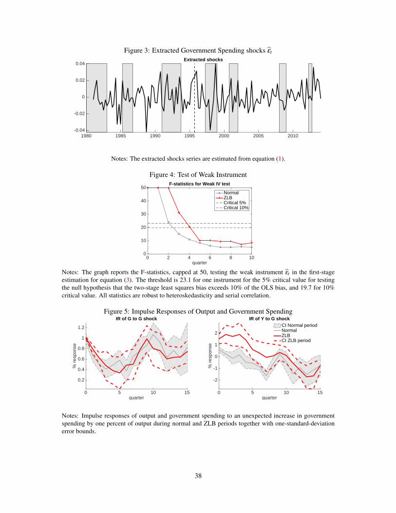
Figure 3 plots the extracted government spending shocks, εt , from equation (1). There is no noticeable dif-

ference between the normal period and the ZLB period in terms of the sizes and the frequency of the shocks.

Additionally, government spending variation during the ZLB period occurs not only during recessions but

also during expansions. The extracted shocks are substantially volatile over time.

Since our extracted government spending shocks εt are the instrument for the estimates of the multipliers

in equation (3), we test whether the instrument is relevant. To take into account possible serial correlations

of the errors, we follow Ramey and Zubairy (2016) and apply the weak instrument tests in Olea and Pfueger

(2013) for every horizons in the normal and the ZLB periods. Figure 4 plots the F-statistics obtained in

the tests along with the thresholds for 5% and 10% critical values for testing the null hypothesis that the

two-stage least squares bias exceeds 10% of the ordinary least squares (OLS) bias.20 In both the normal and

the ZLB periods, the estimated shocks are highly relevant at very short horizons. The F-statistics fall below

the thresholds at horizons longer than one year. This result is consistent with the tests conducted on U.S.

data by Ramey and Zubairy (2016), who also find that the shocks identified from the Blanchard and Perotti

(2002) identification have lower F-statistics at longer horizons. To take into account that the instrument

may be weak at longer horizons, we later test the differences in the output multipliers using both standard

19To the extent that government spending is determined in nominal terms, a large unexpected change in the current price levelcan bias the identification of government spending shocks using nominal government spending deflated by the current price level.We find that the estimated multiplier for the normal period starting in 1973Q1 is slightly higher than the baseline estimates at longerhorizons. However, when we control for this change by deflating nominal government spending by a smoothed measure of inflationor one-quarter lagged inflation, the estimate for the multiplier is similar to that in the baseline.

20The first stage regression includes all the standard controls in four lags.

11

statistics and Anderson and Rubin (1949) statistics.

4.2 Baseline Estimates

We first consider the responses of government spending and output to an unexpected increase in government

spending by one percent of output in period 0. As plotted in Figure 5, output increases on impact and up to

two years in the ZLB period; it increases slightly on impact and then decreases significantly in the normal

period. The one-standard-deviation confidence interval bands for these estimates do not overlap with each

other at shorter horizons. At the same time, the responses of government spending in the normal period are

similar to those in the ZLB period.

To take into account the paths of government spending in the normal period and in the ZLB period,

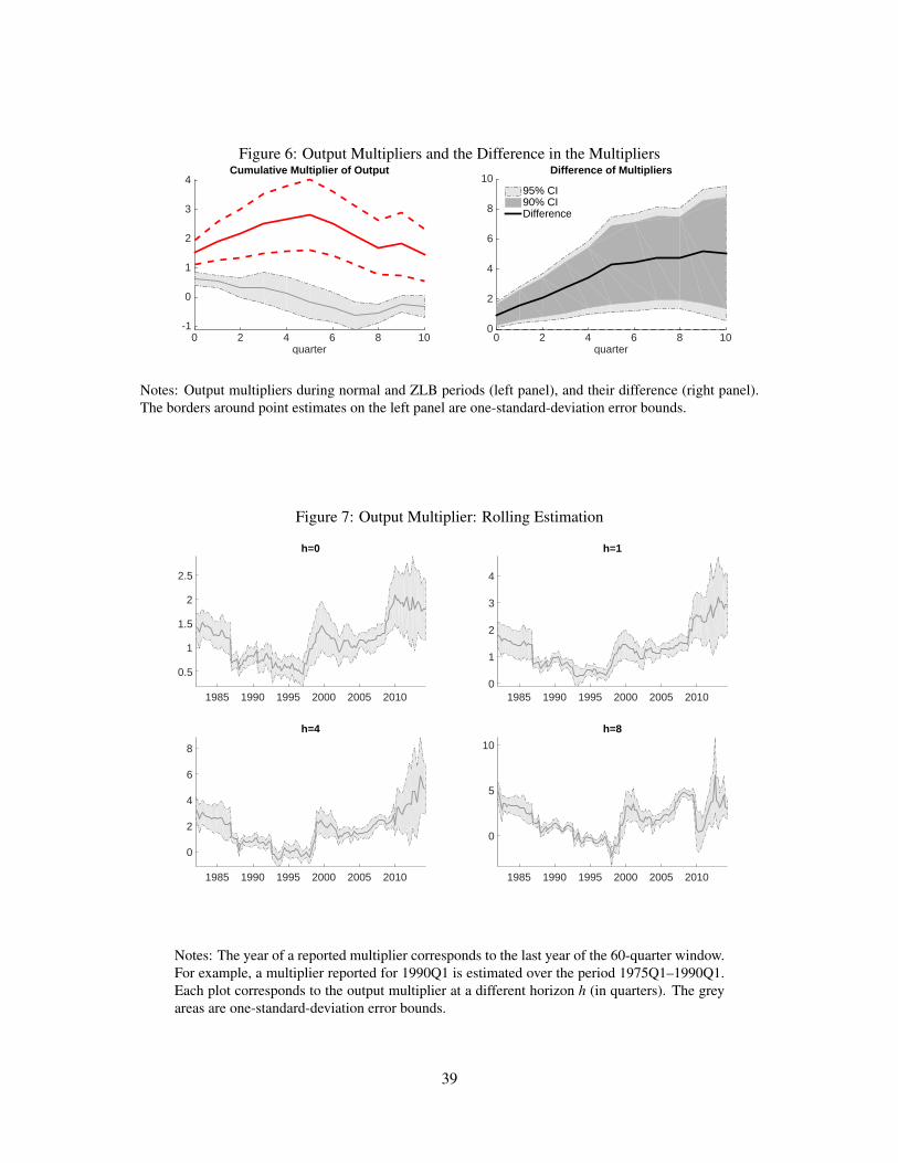
we estimate the output multipliers. Figure 6 plots the output multipliers and their confidence bands in both

normal and ZLB periods. The output multiplier in the ZLB period is significantly larger than zero at all

horizons. It is larger than one and larger than that in the normal period. The output multiplier in the normal

period is 0.6 on impact. This estimate is in line with previous estimates for the United States and other

countries. The output multiplier in the ZLB period is larger: it is 1.5 on impact—more than twice as large as

the on-impact multiplier in the normal period. This multiplier is larger than that documented in the baseline

estimation of Ramey and Zubairy (2016), but it is similar to their estimate when they exclude the World

War II period. The on-impact multipliers in both the normal period and the ZLB period are significantly

larger than zero. The difference between the multipliers in the normal period and in the ZLB period are

pronounced at all horizons. While the output multiplier in the normal period turns negative after the five

quarters, the output multiplier in the ZLB period increases to about two after one year. The one-standard-

deviation confidence bands of the multipliers do not overlap each other. Note that the results of the weak

instrument test suggest that the estimates at longer horizons can be biased.

To formally test whether the multipliers in these two periods are statistically different from each other,

we estimate the following specification:

h

∑j=0

xt+ j = It−1×

[αA,h +MA,h

h

∑j=0

Gt+ j−Gt−1

Yt−1+ψA,h(L)yt−1

]

+(1− It−1)×

[αB,h +MB,h

h

∑j=0

Gt+ j−Gt−1

Yt−1+ψB,h(L)yt−1

]+ ε

xt+h, for h = 1,2, ..., (4)

where It is one if the economy is in the ZLB in period t and zero otherwise, and subscripts A and B indicate

12

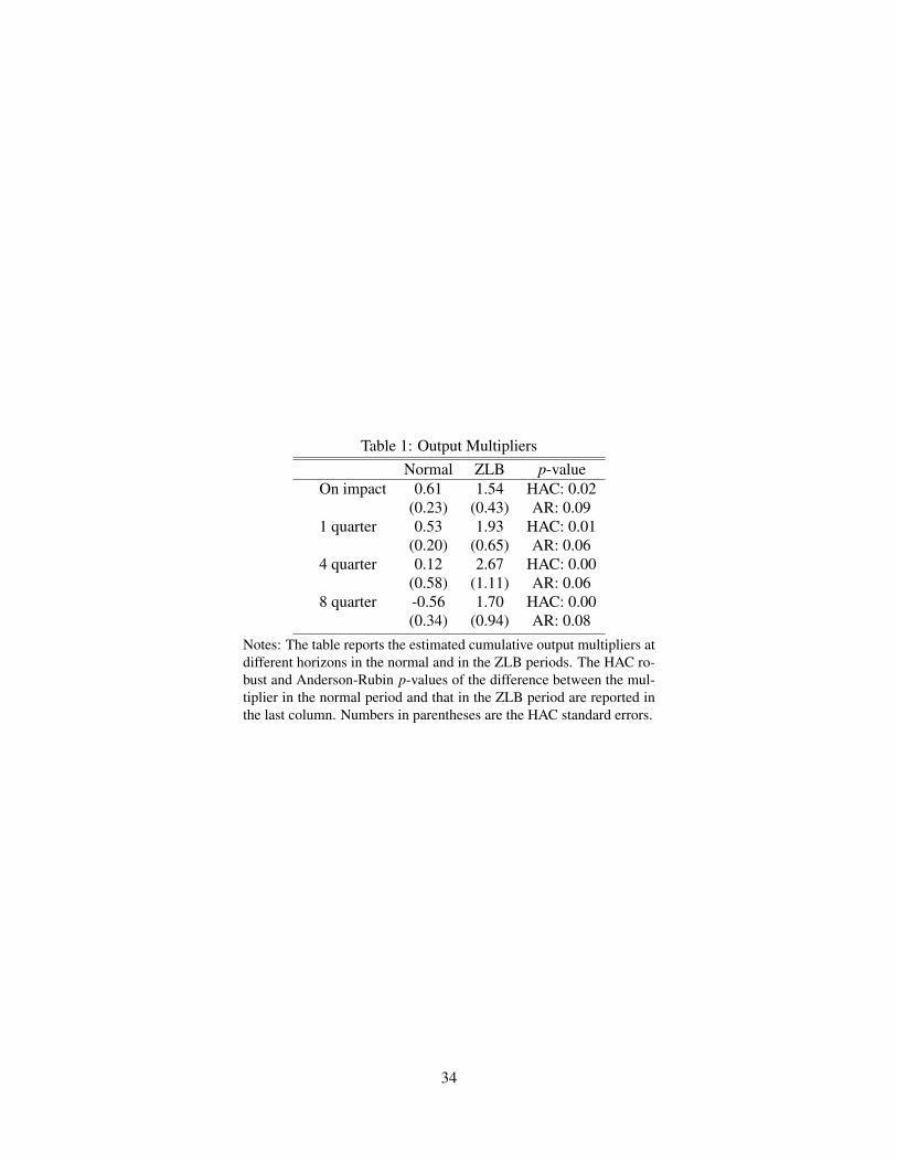
the ZLB and normal periods.21 We test the hypothesis that the multipliers in the ZLB and the normal

periods are the same; i.e. MA,h = MB,h. Table 1 reports HAC p-values for this test at various horizons. We

also include Anderson and Rubin (1949) p-values to account for the fact that the instrument may be weak

at longer horizons. We plot in Figure 6 the differences between the multipliers across all horizons between

zero and 10 quarters and their confidence bands. The 95% confidence interval does not include zero. The

Anderson and Rubin (1949) p-values are slightly higher than the standard p-values, but they are all below

0.1, suggesting that the difference is statistically significant at both short and longer horizons.

4.3 Robustness

This section examines the importance of real-time and other sources of information in estimating the output

multiplier. We also show that the estimated multiplier is robust to other specifications of equation (3).

4.3.1 Importance of Real-time Information

Controlling for forecasts data is important for our analysis. To show this, we compare the baseline estimates

of the output multipliers in the normal period and in the ZLB period with those estimated without forecast

data; i.e., we extract shockt from equation (3) without controlling for forecast.22 The results are displayed in

the first panel of Table 2. Controlling for the information that agents have about future government spending

tends to make the output multipliers larger in the normal period and to a lesser extent in the ZLB period.

This result is similar to the findings for the United States in Auerbach and Gorodnichenko (2012a). Without

controlling for expectations, we would have overstated the effects of government spending in the ZLB period

relative to those in the normal period: government spending is almost five times more expansionary in the

ZLB period than in the normal period on impact. These results suggest that forecast data can change the

estimated multipliers in a non-trivial way and that it is important to control for the expectational effects.23

4.3.2 Additional Predictors of Future Government Spending

Since it is important that we include forecast data in our baseline estimation to obtain unexpected govern-

ment spending shocks, we investigate whether our results are robust to adding more variables to the set of

controls in equation (1).

21Ramey and Zubairy (2016) also use this specification to estimate their state-dependent multipliers. If we use the indicator forthe current period, It , instead of It−1, the results do not change.

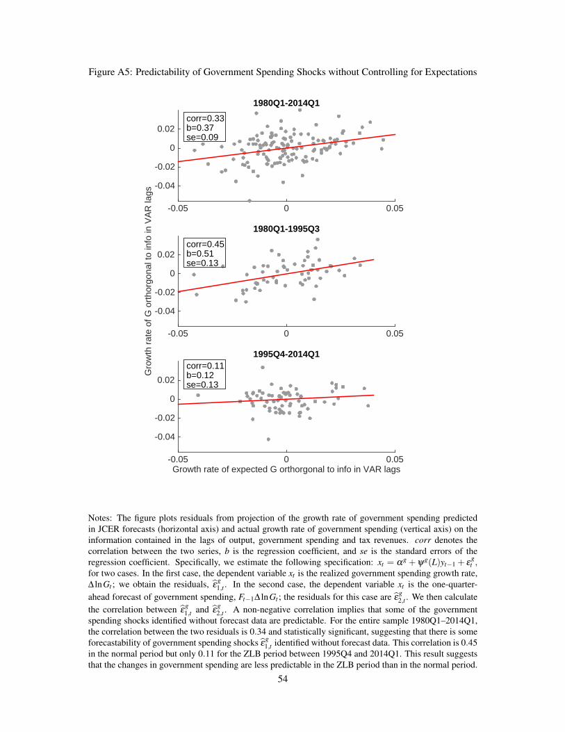
22We plot the estimated multiplier without forecast data and the baseline in Appendix Figure A6.23We also examine the predictability of government spending shocks without controlling for forecast. The results are in Ap-

pendix Figure A5.

13

Other JCER Forecasts. First, we add the government spending component of the fiscal packages ap-

proved by the Japanese government to our first step. These fiscal packages can contain important informa-

tion on the stance of fiscal policy.24 Second, we add a one-year-ahead forecast of the annual government

spending growth rate, Ft∆ lnGt,t+4, to our first step to control for the possibility that agents know the amount

of annual spending but do not know the exact timing. Third, we add one- to four-quarters-ahead forecasts of

the quarterly government spending growth rate. Fourth, we include the one-quarter-ahead forecast of output

as a variable that can summarize the expected future state of the economy. Fifth, we include the one-year-

ahead forecast of the annual output growth rate. Because expected government spending can potentially

react to expected changes in output, it may be important to control for expected output.25

We report in Table 2 the estimated multipliers in these cases.26 The point estimates of the output multi-

pliers in both the normal period and the ZLB period estimated with additional control variables are close to

those in the baseline. The one-standard-deviation confidence intervals for the multipliers in the normal pe-

riod do not overlap with those in the ZLB periods in most cases. Overall, these results suggest that the JCER

forecast of future government spending used in our baseline estimation contains much of the information

present in the additional controls. These results also provide more evidence that the output multiplier in the

ZLB period is substantially different from that in the normal period.

Other Forecast Sources. We next add other sources of forecast into our estimation of unexpected gov-

ernment spending shocks. In particular, the OECD Economic Outlook has released annual forecasts for

government spending in May and November every year since 1983.27 Other sources of government spend-

ing forecast data are the Japanese Cabinet Office’s Economic Outlook database, which contains annual

government spending forecast published in December from 1980, and the quarterly IMF forecast, which

starts in 2003.28 We re-estimate equation (1) to include all of the available one-quarter-ahead forecasts of

24The Japanese government implements fiscal packages from time to time. These packages often contain several measures suchas tax cut, spending, and special transfer. We use the spending component of these packages when these fiscal packages are passed.We also use the information from the supplementary budget for the central government, which is additional budget items approvedduring a fiscal year. Appendix Figure A2 plots these data for the supplementary budget and fiscal packages as a percentage of GDP.The estimated multipliers when these data are added as controls are similar to the baseline.

25We perform several additional robustness exercises. We include other variables that can contain important information aboutpublic investment. For example, we add four lags of contracted public work orders, orders received for public construction, andthe excess returns of construction sector stock prices to control for expected government investment. We also considered variablesthat can include information on the state of the economy and the fiscal stance, such as real exchange rates and the index of leadingindicators. The results remain similar to the baseline estimates. In Appendix Figure A4, we report the estimates of cumulativemultipliers of output in the specification with orders received for public construction and contracted public work orders.

26We plot the results at all horizons in Figure A3.27We thank Yuriy Gorodnichenko for providing us with the OECD and IMF data.28We plot in Figure A1 the actual cumulative growth rate of government spending along with its one-quarter-ahead forecasts

from the JCER, the OECD, and the Japanese Cabinet Office’s Economic Outlook. This plot suggests that the JCER and the OECDforecasts track the actual government spending well before 2000 but less so after 2000.

14

government spending from these sources and compute the multipliers for different horizons in the second-

to-last panel of Table 2. The multipliers in the normal period estimated with additional data are similar

to those in the baseline. Although the estimates for the multipliers in the ZLB period are slightly higher

than the baseline, the difference is small. The differences between the multipliers in the ZLB period and

in the normal period are significant at shorter horizons. Overall, these results are in line with the baseline

estimation.

4.3.3 Variations of the Baseline Specification

We show that the baseline results are robust to other estimation specifications.

First, we estimate a version of specification (2) with a quadratic trend since time series estimates can

be sensitive to trends. The last three rows of Table 2 displays the output multipliers in this case. We find

that the multipliers estimated with a trend are similar to those in the baseline, although the output multiplier

estimated with a trend in the normal time is somewhat larger at longer horizons than in the baseline.

Second, we perform an alternative transformation of government spending and output by dividing them

by potential output to calculate the multipliers. The motivation for this approach is as follows: In our

baseline estimation, we convert government spending from the percentage changes to dollar changes using

the value of the government spending–output ratio at each point in time, rather than using sample averages.

A potential problem of the baseline transformation is that the cyclicality of output can bias the estimated

multiplier. Formally, we estimate equation (3) for (Yt+h−Yt−1)/Y t−1 and (Gt+h−Gt−1)/Y t−1, where Y t is

potential output, computed using the Hodrick-Prescott (HP) filter.29 The multipliers estimated in this case,

reported in Table 2, are essentially the same as our baseline.

Third, one potential concern with our estimation is that we use the residuals εt of equation (1) to proxy

for shockt without taking into account the uncertainty of the estimates. We address this concern and im-

plement a one-step estimation of the effects of unexpected government spending on output. Formally, we

estimate the following version of equation (3):

h

∑j=0

xt+ j = αxh +Mh

h

∑j=0

Gt+ j−Gt−1

Yt−1+ γ

xhFt−1∆ lnGt +ψ

xh(L)yt−1 + ε

xt+h, for h = 0,1,2, ...

where we instrument ∑hj=0

Gt+ j−Gt−1Yt−1

with current growth rate of government spending because the regression

includes both forecast and lags of control variables. This approach has the same interpretation as our two-

step procedure. The results obtained from this estimation are shown in Table 2. The multipliers are virtually

29We set the smoothing parameter to be 1600.

15

identical to our baseline estimates. The standard errors of the one-step and the baseline estimations are also

similar.

Finally, we estimate a 15-year rolling-window regression version of our baseline specification between

1967Q1 and 2014Q1. Figure 7 plots the multiplier at different horizons. The multiplier is time-varying.

Between 1967 and 1984, the cumulative output multiplier is about 1.2 on impact and increases to about 3

at a two-year horizon. This result shows that the multiplier can be larger than one during the 1960s and

1970s when the Japanese economy was under the fixed exchange rate regime. After the collapse of the fixed

exchange rate regime, the multiplier is below unity for all years up to 1997. This result is consistent with the

finding in Ilzetzki, Mendoza, and Vegh (2013) that the multiplier is larger in the fixed exchange rate regime

than in the flexible exchange rate regime. The multiplier becomes higher than unity starting in 1995. This

tendency is similar across all horizons. Overall, the rolling regression results are consistent with our baseline

estimates and suggests that the multiplier is larger in the ZLB period than in the period before 1995.30

5 The Multipliers of Other Variables

We have shown that the output multipliers are different in the ZLB and normal periods. It is natural to expect

that the difference should be reflected in the responses of components of output and other variables related

to output. In this section, we examine the multipliers of private aggregate consumption, investment, and the

unemployment rate in the ZLB period and compare them with those in the normal period.31

5.1 Private Consumption and Investment

The effects of government spending shocks on private consumption and investment can be estimated by

applying (3) for consumption and investment. For example, the consumption multiplier can be estimated by

the following set of IV regressions:

h

∑j=0

Ct+ j−Ct−1

Yt−1= α

Ch +MC

h

h

∑j=0

Gt+ j−Gt−1

Yt−1+ψ

Ch (L)yt−1 + ε

xt+h, for h = 0,1,2, ..., (5)

30We also estimate the output multipliers from a five-variable SVAR. The five variables are forecast of government spending,government spending, tax revenue, output growth rates, and the unemployment rate. We include four lags in the SVAR, similar tothe baseline. The estimated output multipliers in both the ZLB period and the normal period are plotted in Appendix Figure A7.The SVAR results are similar to the baseline estimation using the local projection method. The differences in the multipliers arealso statistically significant as in the baseline estimation.

31We also estimate the multipliers for net exports and the real effective exchange rate in Japan. The results are reported inAppendix Figure A11.

16

where the instrument for the cumulative changes in government spending is shockt . We add four lags of

consumption to the vector of standard controls. The private investment multiplier are estimated and defined

in the same manner.32

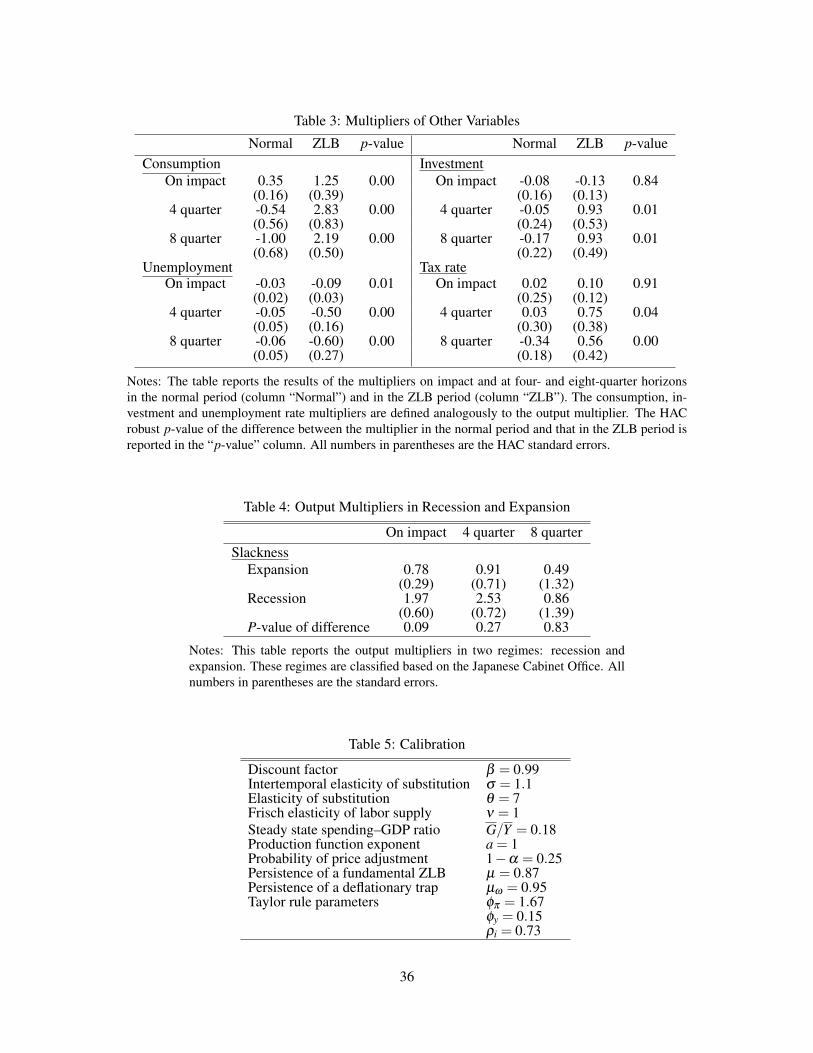
Figure 8 plots the cumulative multipliers of consumption and investment to government spending at all

horizons. The multiplier for consumption is positive and significantly different from zero in the ZLB period;

it is negative and statistically different from zero in the normal period at a one-year and a two-year horizon.

The investment multiplier in the ZLB period is also positive and higher than that in the normal period at

most horizons other than on impact. As indicated by the p-value of the differences in the multipliers in

the two periods in Table 3, the consumption multiplier is significantly larger in the ZLB period than in the

normal period, at 1% significance level. The difference in the investment multipliers is not significant on

impact, but it is statistically significant with the p-value of about 0.01 after four and eight quarters.33

5.2 Unemployment

We examine the responses of the labor market to a government spending shock by estimating a version

of equation (3) for the unemployment rate. The multiplier of the unemployment rate is defined as the

cumulative percentage point changes in unemployment rate in response to a change in government spending

by one percent of output at each horizon, in the ZLB period and in the normal period.34 We plot the

cumulative multipliers of the unemployment rate in Figure 9. During the normal period, the unemployment

rate does not respond much after an increase in government spending by one percent of output. In contrast,

in the ZLB period, the unemployment rate decreases substantially by 0.1 percentage point on impact and

further to 0.5 percentage point a year after an increase in spending by one percent of output. The drop in the

unemployment rate in the ZLB period is significantly different from zero at all horizons. Furthermore, the

confidence intervals of the unemployment rate multipliers in the ZLB and the normal periods do not overlap

across all horizons. We formally test the difference in the unemployment rate multipliers and report in Table

A1. We find that the difference is significant at the 5% level at horizons between one and eight quarters after

32Private consumption is the final consumption including transfer from the government. Private investment is the sum ofresidential and nonresidential investment. The results are the same if we use the final consumption data without transfer from thegovernment.

33We also estimate the multipliers for components of consumption and investment including durables, nondurables, semi-durables, and services consumption as well as residential and non-residential investment using the same specification. The resultsare reported in Appendix Figure A12.

34This measure of the multiplier is analogous to our definition of the output multiplier. Alternatively, one can define the unem-ployment multiplier by the absolute change in the unemployment rate after h quarters normalized by the cumulative governmentspending changes. Both measures of unemployment multipliers imply significantly different behavior of the unemployment ratein the normal and the ZLB periods. See Monacelli, Perotti, and Trigari (2010) for more on empirical and theoretical analyses ofunemployment multipliers.

17

the shock.

To sum up, using Japanese data between 1980Q1 and 2014Q1, we find that:

1. The output multiplier in the ZLB period is larger than that in the normal period. Government spending

is more than twice as expansionary in the ZLB period as in the normal period.

2. Government spending crowds private consumption and investment in during the ZLB period, but it

crowds them out in the normal period.

3. The unemployment rate decreases in the ZLB period significantly more than in the normal period after

a government spending shock.

6 What Explains Larger Multipliers at the Zero Lower Bound?

We investigate several hypotheses that can explain the larger multipliers in the ZLB period. We first examine

the mechanism in New Keynesian models by documenting the effects of government spending on inflation,

expected inflation and nominal interest rates. We then discuss whether the effects of government spending

in recessions, or the differences in the tax rates in the two periods can explain our empirical findings. We

relax the Blanchard-Perotti identification assumption to examine how it may explain the differences in the

multipliers in the two periods. Lastly, we show that the composition of government spending in the two

periods may not explain the difference in the multipliers.

6.1 The New Keynesian Mechanism

A typical New Keynesian model provides a possible explanation for the difference between the multiplier in

the ZLB period and that in the normal period: the short-term nominal interest rate net of expected inflation

goes up in the normal period but drops in the ZLB period. In this section, we document the responses of

inflation, inflation expectations and the nominal interest rate after a government spending shock to shed

light on the New Keynesian mechanism. In Section 7, we examine whether a simple New Keynesian model

calibrated using Japanese data can reproduce these empirical findings.

Denoting inflation by πt , we estimate the multipliers of inflation to government spending shocks from

equation (3) with the variable of interest xt+ j being the inflation rate πt+ j, and the vector of controls includes

four lags of the inflation rate, the standard controls and the five-year nominal interest rate.35 We estimate

35The results do not change if we use other nominal interest rates or the yield of the 10-year bond. The results also do notchange if we do not include current interest rate in the controls.

18

the responses of both GDP deflator inflation and CPI inflation.36

We find mixed evidence on the response of inflation to unexpected government spending shocks: while

the responses of the GDP deflator inflation are mild and not statistically different from zero in both the

normal and the ZLB periods at the short horizons, the responses of CPI inflation are more significantly

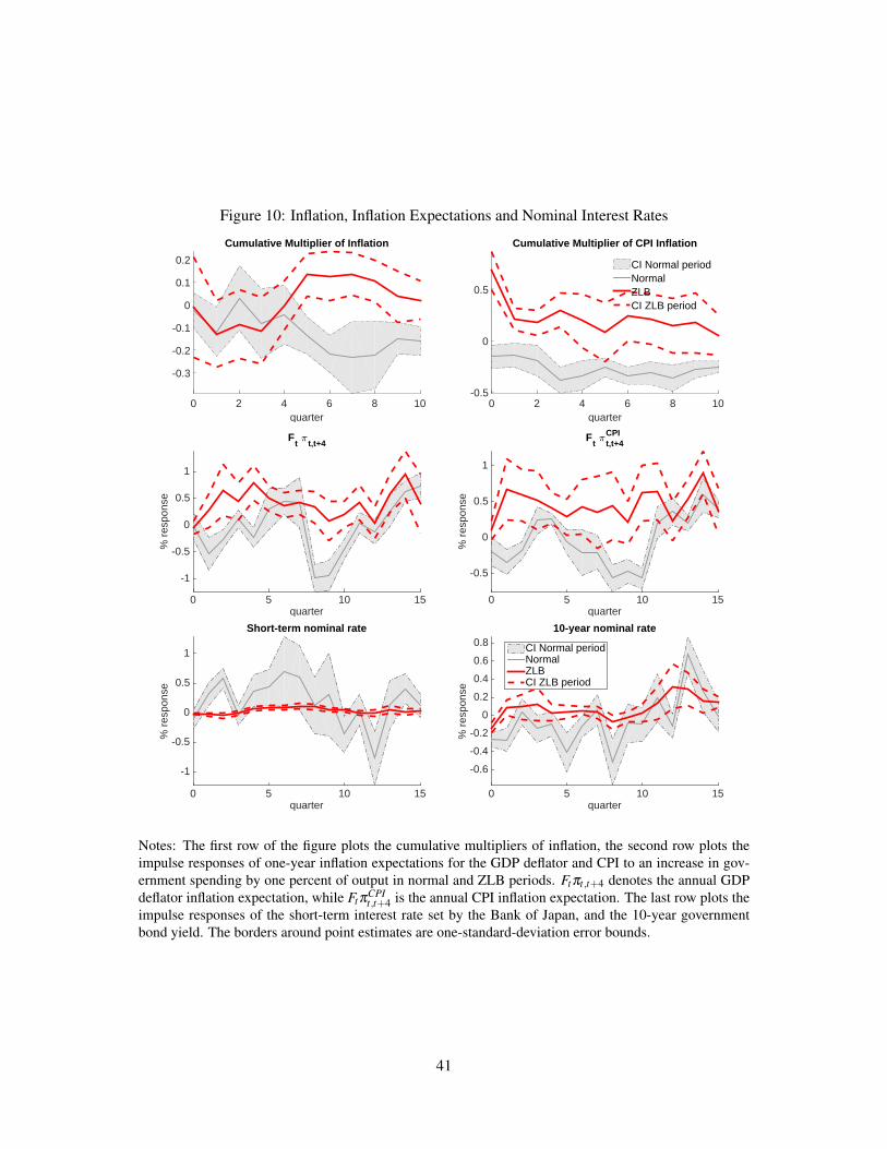
positive in the ZLB period than those in the normal period. Figure 10 plots the multipliers of these two

measures of inflation in both the normal and the ZLB periods. Inflation calculated from the GDP deflator

responds little to a positive government spending shock in both periods, on impact. The cumulative inflation

multiplier is about 0.1 percentage points at a two-year horizon in the ZLB period but negative in the normal

period. Overall, the response of inflation is mild in both periods, and the confidence intervals include zero

at short horizons. The multipliers of CPI inflation are, however, significantly more positive than those of

inflation calculated from the GDP deflator in the ZLB period. CPI inflation in the ZLB period responds

more positively and is significantly larger than zero on impact: an increase in government spending by one

percent of output leads to a 0.68 percentage point increase in CPI inflation in the ZLB period on impact.

The response of CPI inflation in the normal period is −0.16 percentage points.37 This result suggests that

there is some evidence of a positive inflation response in the ZLB period.

The differences of the responses of the four-quarters-ahead annual inflation forecast in the ZLB period

and in the normal period are more pronounced. In the estimation, we control for four lags of the dependent

variables, the standard controls and the five-year nominal interest rate. Figure 10 plots the responses of

the four-quarters-ahead expected annual inflation calculated from both a forecast of the GDP deflator and

the CPI to an increase in government spending by one percent of output. The on-impact responses of

inflation expectations calculated from the GDP deflator are negative but statistically insignificant in both

the normal period and the ZLB period. Inflation expectations are negative in the normal period, while they

are positive in the ZLB period in the next two quarters. Inflation expectation increases by 0.65 percentage

points after two quarters in the ZLB period but decreases by 0.25 percentage points in the normal period. The

differences between inflation expectations in the normal period and those in the ZLB period are also present

when we look at the CPI. The on-impact responses of the CPI inflation expectations are not statistically

36The inflation multiplier is essentially the impulse response of nominal price index divided by the cumulative change in gov-ernment spending.

37To examine the robustness of the response of CPI inflation in the normal period and in the ZLB period, we estimate theresponses of core CPI inflation. Furthermore, since both total CPI and core CPI are affected by the consumption tax hikes in 1989and 1997, we consider the responses of inflation adjusted for these consumption tax changes following Hayashi and Koeda (2014):We adjust the annual inflation rates from April 1989 to March 1990 and from April 1997 to March 1998 for the consumption taxincreases, then recover the CPI level consistent with the adjusted annual inflation rates. The responses of inflation calculated fromthese series are plotted in Figure A10. The inflation responses using either tax-adjusted inflation or the core CPI resemble thebaseline. The tax-adjusted CPI inflation responses are positive and significant on impact in the ZLB period. When food and energyare excluded, the core CPI inflation also increases significantly in the ZLB period on impact.

19

significantly different from zero in both periods. However, at horizons 1 and longer, the CPI inflation

expectation responses are positive and significantly different from zero in the ZLB period, but are negative

in the normal period. We reject the joint null hypothesis that the responses of inflation expectations (both

GDP deflator and CPI) at all horizons do not differ across the two subsamples at the 5% confidence level.

The last panel of Figure 10 plots the impulse responses of the overnight (short-term) nominal interest

rate and the yield on a 10-year government bond to an increase in government spending by one percent of

output, respectively. These responses are estimated by adding to the baseline specification (2) four lags of the

dependent variable, the standard controls and the inflation rate. We include trendt to control for the observed

decline in the nominal interest rate over time.38 We report the results estimated with a quadratic trend, but the

results do not change if we include a linear trend. In the normal period, the short-term interest rate increases

to 0.37 percentage points for a one-year horizon in response to an increase in government spending by

one percent of output. In the ZLB period, the short-term interest rate does not react to government spending

shocks, consistent with the idea that the central bank is not responsive to government spending shocks during

the ZLB period. These results together with the response of expected inflation suggest that the short-term

real interest rate increases more in the normal period than in the ZLB period.

We note that the response of the 10-year nominal interest rate is generally not statistically different

from zero, and increases after 10 quarters in both the normal and the ZLB periods. Additionally, the point

estimates of the response of the long-rates is higher in the ZLB period than in the normal period. This

behavior of the long-term nominal interest rate is at odds with a simple linearized New Keynesian model

in which expectation hypothesis holds. A richer model with bonds risk and term premia can potentially

rationalize our long rates estimates.

6.2 Output Multipliers in the ZLB Period and in Recessions

Recent studies by Auerbach and Gorodnichenko (2012a,b) find that the output multiplier is larger than one

in recessions and smaller than one in expansions using U.S. and OECD data. As the ZLB period often

coincides with recessions, it is important to differentiate evidence from the ZLB period and evidence from

recessions. This section shows that our estimated multiplier in the ZLB period may not be attributed to the

large effects of government spending in recessions. We also examine the possibility that the whole ZLB

period coincides with a long period of elevated slack, which can also potentially explain our results.

We first estimate the multipliers during booms and recessions in Japan between 1980Q1 and 2014Q1

38There is a clear trend in the nominal interest rate in the normal period. If we exclude trend in the specification, as reportedin Appendix Figure A13, the main difference from our results here is that the responses of the nominal interest rate in the normalperiod are not as positive. Note that we do not include trend in other variables since adding trend does not alter the results.

20

by estimating a state-dependent version of the specification in equation (4), similar to Ramey and Zubairy

(2016).39 The recession indicator is based on the Cabinet Office of Japan classification of trough periods.

Figure 11 plots the output multipliers in recessions and expansions and the difference between these two

multipliers. The on-impact output multiplier in recessions is as large as 2.3, and it is 0.8 in expansions.

The differences in the multipliers in recessions and in expansions are smaller at horizons longer than three

quarters. The differences are also not statistically significant at longer horizons, as reported in Table 4. This

result for Japan is qualitatively similar to that for the United States in Auerbach and Gorodnichenko (2012a)

but weaker in significance. The results in this section do not change if we use the peak-to-trough recession

classification by the OECD.

Since the multiplier in recessions is larger than that in expansions, to explain the larger multiplier in the

ZLB period, we would need more recessions in the ZLB than in the normal period. However, this is not the

case. Japan is not always in recession during the ZLB period 1995Q4 and 2014Q1, as can be seen in Figure

1. The number of quarters in recession are slightly higher in the normal period than in the ZLB period: 45%

of the quarters in the normal period are in recession, but only 30% in the ZLB period are. This implies that

the multiplier during the ZLB period should be smaller than the multiplier during the normal period if the

only fundamental difference is between the values of the multipliers in recessions and expansions. More

precisely, the extracted shocks plotted in Figure 3 suggest that most government spending variations during

the ZLB do not occur during recessions, and most government spending variations during the normal period

do not occur during booms. Therefore, it is unlikely that the difference in multipliers across recessions and

booms can explain the difference in multipliers between the ZLB and normal periods that we estimate.40

Our analysis does not rule out the possibility that a long period of slack, coinciding with the ZLB

period, can potentially explain the estimated high output multiplier in the ZLB period. As plotted in Figure

12, the unemployment rate, which is sometimes used as a measure of slack, is permanently higher during the

ZLB period than the normal period. However, we note that one should use labor market tightness, not the

unemployment rate, as an indicator of slack that explains the multipliers. There is no evidence that tightness

changed permanently (see Figure 13).

The fact that tightness and not unemployment is the relevant measure of slack which affects the size of

multipliers comes from the leading theoretical model (Michaillat, 2014). The intuition is based on a standard

search-and-matching labor market model: In states with high tightness, government purchases crowd out

39We also estimate the multipliers in recessions and booms in each subperiod but the confidence interval is large due to the smallsample, especially for recessions.

40It is possible that the multiplier is bigger in deeper recessions. However, it is not the case that Japan has experienced moresevere recessions during the ZLB period than in the normal period.

21

private employment more than in states with low tightness. The government spending multiplier, therefore,

is lower when tightness is higher. In addition, following shifts in the Beveridge curve, unemployment can

vary for given tightness and, hence, multipliers.

While it is clear that the unemployment rate was substantially higher in the ZLB period in Japan, there

is no apparent break in tightness that would signal the permanently higher amount of slack after 1995, as

plotted in Figure 13. One possible explanation for this is the series of labor market reforms in the 1990s

and 2000s that deregulated fixed-term labor contracts and likely shifted the Beveridge curve out, increasing

frictional unemployment without affecting tightness permanently (Hijzen et al., 2015). This again suggests

that tightness, and not unemployment, is a better proxy for labor market slack in Japan.41

6.3 Tax Rate

Another possible explanation for the difference in the output multipliers in the ZLB period and in the normal

period is that tax rates respond differently in the two periods. We estimate the responses of average tax rates

in the normal period and in the ZLB period after a government spending shock. We define the average tax

rate Tt as a ratio of tax revenues to GDP. The cumulative multipliers of the average tax rate are estimated

from equation (3), with the variable of interest Tt+h. We plot the multipliers of the average tax rate in the

last panel of Figure 9. We find that in response to an increase in government spending by one percent of

output, the average tax rate increases in both the normal period and the ZLB period. The increase in the tax

rate is larger in the ZLB period than in the normal period at horizons longer than one year. For example, the

cumulative response of the average tax rate is 0.5 percentage points in the ZLB period after two quarters,

and it is near zero in the normal period. At longer horizons, the cumulative responses of the average tax rate

is more negative in the normal period than in the ZLB period. This result suggests that to the extent that tax

is contractionary, the different responses of the average tax rate in the two periods are not likely to explain

the observed difference in the output multipliers.

6.4 Automatic Stabilizer

To obtain our main results, we assumed that variations in output do not automatically change current govern-

ment spending; i.e., the elasticity of government spending with respect to current output ηG,Y is zero. The

idea behind this assumption, as Blanchard and Perotti (2002) discuss, is that the government needs some

time to change government spending in response to current economic conditions. To examine whether this41This discussion does not mean to imply that the recent papers that estimated state-dependent multipliers in the US data using

unemployment as an indicator of slack are wrong. The reason is that in the US, unlike in Japan, unemployment behavior mirrorstightness behavior.

22

assumption can explain the difference in the multipliers between the ZLB period and the normal period, we

assume a non-zero elasticity of government spending to current output. Specifically, we change the first step

of our empirical procedure, equation (1), as follows:

∆ lnGt = α +ηG,Y ∆ lnYt + γFt−1∆ lnGt +ψ(L)yt−1 + εt ,

and fix ηG,Y to be either−0.1 or 0.1. Consistent with the analysis of Caldara and Kamps (2012), we find that

the on-impact multiplier is lower than our baseline estimates when ηG,Y = 0.1. The on-impact multipliers

in the ZLB and normal periods are 1.4 and 0.5, respectively.42 The on-impact multipliers in both periods

are higher than the baseline when the elasticity, ηG,Y = −0.1: 1.7 in the ZLB period and 0.7 in the normal

period, respectively. This result suggests that our estimated output multiplier is biased if the true elasticity

ηG,Y is non-zero. However, this bias has the same sign and approximately the same size across the ZLB and

normal periods. As a result, the failure of the Blanchard and Perotti (2002) identification assumption alone

may not explain the difference in the estimated output multipliers across the normal and ZLB periods.43

6.5 Composition of Government Spending

Another potential explanation for the difference in the multipliers between the ZLB period and the normal

period is that the investment-consumption composition of government spending has changed over time.

To examine this explanation, we document the responses of government investment and consumption to

government spending shocks and plot the results in Figure 14. In response to an increase in total government

spending by one percent of output, government investment increases by 0.8 percent of output on impact for

both the ZLB period and the normal period. The paths of the responses of government investment are similar

across the two periods. The paths of government consumption are also similar across these two periods with

an increase of about 0.2 percent of output on impact.

If there was a substantial difference in the responses of public consumption and/or public investment

after a government spending shock in the normal and in the ZLB periods, this could potentially account for

some difference in the multipliers that we estimate. However, given that there is no big difference in the

responses, this is not likely to explain the difference in the output multipliers that we estimate.

42Caldara and Kamps (2012) analyze the relationship between fiscal multipliers and the output elasticity of fiscal variables.43Only when we assume substantially different elasticities in the ZLB period and in the normal period can the automatic

stabilizer effect alone explain the difference between the estimated output multipliers. We find that ηG,Y should be −0.7 in thenormal period for the on-impact multiplier in the normal period to be almost the same as our baseline on-impact multiplier in theZLB period (1.5). Alternatively, if ηG,Y = 0.5 in the ZLB period, the on-impact multiplier in the ZLB period equals the on-impactoutput multiplier in the normal period in our baseline estimation (0.6).

23

7 A Model of Government Spending

A possible explanation for our empirical findings of a higher output multiplier in the ZLB period is the

New Keynesian mechanism. However, the predictions about the sign and the size of the multipliers in

New Keynesian models depend crucially on several conditions, e.g, the relative duration of government

spending shocks and ZLB period. This section seeks to understand if and under what conditions a simple

New Keynesian model calibrated with Japanese data can match the empirical results. We find that the model

can replicate some of our empirical findings if the ZLB period is driven by a deflationary trap, and the

government spending process is not too persistent. At the same time, the model with the ZLB period caused

by a fundamental shock misses all of our empirical estimates. We discuss some extensions of the model that

can better explain the data.

We examine a standard New Keynesian model along the lines of Woodford (2010), Eggertsson (2011),

and Christiano, Eichenbaum, and Rebelo (2011).44 The full model description can be found in Appendix

A.1. In this model, there is a continuum of household types, each of which consumes, and supplies a

differentiated labor input. The model features monopolistic competition and Calvo-style sticky prices. There

is no capital investment. The government finances wasteful spending through lump-sum taxes. The model

equilibrium conditions log-linearized around a zero-inflation steady state can be summarized by the IS and

the Phillips curves:

yt − gt = Et (yt+1− gt+1)− σ (it −Etπt+1− r) , (6)

πt = βEπt+1 +κ (yt −Γgt) , (7)

where t indexes a model time period which corresponds to one quarter, yt denotes the log deviation of output

from its steady state, gt denotes government spending deviation from its steady state over steady state output,

πt is inflation, it is a continuously compounded one-period riskless nominal interest rate, and r is the value

of this rate in a steady state with zero inflation. The constant κ is the slope of the Phillips curve, Γ is the

44Instead of comparing our empirical results to the prediction of the full New Keynesian model, one could potentially use ourconsumption and price level impulse responses to check if they are consistent with the Euler equation that takes the following formin the ZLB: ct = Etct+h + σEt(pt+h− pt)+ t.i.p., where t.i.p. collects the terms that do not depend on fiscal policy. We do notfollow this path here, because we do not directly observe the expectations of future consumption or price level responses. Instead,our estimation only provides us with the responses of these variables conditional on staying in the ZLB period. Interpreting ourconditional estimates as expectations of variables is akin to assuming that the economy is expected to stay in the ZLB forever.However, the long-term government bond yields net of term premium are above zero in Japan during the ZLB period (see footnote52). This suggests that the market participants in Japan expected an increase in monetary policy rate in the future. Moreover, to usethis method in the normal period, we would still need to make assumptions about the behavior of monetary policy.

Note that when we, nevertheless, assume that our impulse responses measure the expected path of consumption and price level,we can use the Euler equation to back out σ . We can do this exercise for all horizons h for which we estimate the responses.The median value of backed-out σ over horizons 0–15 is 1.79 with wide standard deviation bounds that include the value in ourcalibration of σ = σ ·C/Y ≈ 0.9.

24

fiscal multiplier under flexible prices, and σ is the “effective” intertemporal elasticity of substitution.45

We characterize government spending policy by a steady state ratio of government spending over GDP,

and by the path of government spending after a government spending shock. We assume that government

spending after a spending shock equals the point estimate of the empirical impulse responses for the first

sixteen quarters; then government spending reverts to steady state according to an AR(1) process. Formally,

gt = gempt for 0 ≤ t ≤ 15, and gt = gemp

15 · ρ t−15 for t > 15, where gempt is our empirical point estimates.

Because the empirical responses of government spending to a government spending shock are very close to

each other in the normal and the ZLB periods, we use the normal period response as gempt .

We define the output multiplier analogous to its empirical counterpart: Myh = ∑

ht=0 yt/∑

ht=0 gt . We intro-

duce the cumulative inflation multiplier and define it similarly to the output multiplier: Mπh =∑

ht=0 πt/∑

ht=0 gt .

To examine the theoretical multipliers in the normal and in the ZLB periods, we consider three scenarios:

(i) an unconstrained monetary policy that follows a Taylor rule, (ii) the zero interest rate period caused by a

fundamental shock to the spread between the monetary policy rate and the interest rate that the households

face, (iii) the zero interest rate period caused by self-fulfilling periods of low confidence.

7.1 Normal Period

We model the normal period by assuming that monetary policy follows the Taylor rule of the following form

it = (1−ρi)(r+φππt +φyyt)+ρiit−1, (8)

where r ≡− logβ , φπ > 1, φy ≥ 0, and 0 < ρi < 1. We assume that the economy never reaches the ZLB in

this case. We solve the model for a unique bounded equilibrium. The details are in Appendix A.3.

7.2 ZLB due to Fundamental Shocks

One way to generate a zero nominal interest rate period is to assume the occurrence of a fundamental shock

that requires the central bank to lower its policy rate to the lowest possible level. We follow Woodford

(2010) and Eggertsson (2011) by allowing the policy interest rate to differ from the interest rate faced by the

households. The Euler equation (6) becomes

yt − gt = Et (yt+1− gt+1)− σ(it −Etπt+1− rnet

t), (9)

45κ,Γ, σ are expressed through the model’s structural parameters in Appendix A.2.

25

where rnett ≡ r−∆t , and ∆t represents a spread between the policy rate and the interest rate that is relevant

for the intertemporal consumption allocation of the households. Intuitively, a positive ∆t may stand for a

temporary disruption of the intermediation in the financial sector.

As in Woodford (2010), we consider a simple two-state Markov example in which rnett takes only two

values: r and rL, where rL < r. If the economy starts from a state with the elevated spread, i.e., rnett = rL,

then it stays in the same state in the next period with probability µ; otherwise, it returns to a zero-spread

state, i.e., rt = r, with probability 1−µ . Once the spread returns to normal level, it stays there forever. If the

monetary policy follows the Taylor rule, (8) a large enough spread shock, i.e., small enough rL, will imply

negative it . As a result, the ZLB on the nominal rate starts to bind. Once the spreads normalize, the central

bank follows the Taylor rule again.

We solve the model for a unique bounded equilibrium. The uniqueness assumption puts an upper bound

on the persistence µ of interest rate spread shocks.

7.3 ZLB due to Non-fundamental Shocks

Self-fulfilling variations in confidence provide an alternative explanation for the occurrence of the ZLB

periods.46 There are two steady states in the standard New Keynesian model when the policy rate follows a

Taylor rule with ZLB constraint: the standard targeted inflation steady state and a “deflationary trap” steady

state with zero nominal interest rate and deflation (Benhabib, Schmitt-Grohe, and Uribe, 2001a,b).47 In the

neighborhood of the deflationary trap steady state, there are infinitely many equilibrium paths leading to

this steady state, implying infinitely many responses to a government spending shock. We follow Mertens

and Ravn (2014) and Aruoba, Cuba-Borda, and Schorfheide (2016) and restrict our attention to Markov

equilibria in which the only state variables are a non-fundamental random variable, called a sunspot, the

current value of exogenous government spending, and a set of current news shocks about future government

spending that replicate the empirically estimated government spending expected by the agents in advance.48

This form of equilibrium restricts the solution to a single equilibrium: a sunspot determines a steady state

to which the economy approaches; the Markovian structure with respect to exogenous fundamental shocks

46In a recent paper, Aruoba, Cuba-Borda, and Schorfheide (2016) estimate a New Keynesian model and conclude that Japan ismore likely to be at the ZLB because it is experiencing a low level of confidence rather than a liquidity trap caused by fundamentalshocks. This provides a rationale to investigate government spending multipliers in this situation. Schmitt-Grohe and Uribe (2016)show that a New Keynesian model with a confidence-driven ZLB period and downward nominal wage rigidity can generate botha persistent ZLB period and persistent increase in the unemployment rate, consistent with the recent experience in Japan. In thecurrent paper, we study only Calvo-style nominal price rigidities.

47Intuitively, if agents believe that there is permanent deflation, the central bank sets the nominal rate to zero. If the level ofdeflation equals the subjective discount factor, the economy can remain in this equilibrium forever. Thus, the economy may end upin a deflationary steady state with zero nominal interest rate because agents unexpectedly change their beliefs.

48In a non-linear solution to the model, the price dispersion will be an additional state variables.

26

pins down a unique response of the economy to shocks.49 We assume that government spending shocks do

not affect sunspots.

Formally, a sunspot, represented by variable ωt , can take on two values {ωP,ωO}. We call ωO a state

with “optimistic” expectations and ωP a state with “pessimistic” expectations because, by assumption, the

economy converges to the desirable targeted inflation steady state when ωt = ωO and to the deflationary

steady state when ωt = ωP. The optimistic expectations state is absorbing: Pr (ωt = ωO|ωt−1 = ωO) = 1.

If the economy starts in a state with pessimistic expectations, the probability to remain in this state in the

next period is Pr (ωt = ωP|ωt−1 = ωP) = µω ∈ [0,1]. We solve the model by log-linearizing the equilibrium

conditions around the zero-inflation steady state. See the appendix for details.50

7.4 Calibration

We set the values of the parameters as in Table 5. The Frisch elasticity of labor supply ν is 1, which is the

standard value used in the macroeconomics literature. The elasticity of intertemporal substitution (IES) σ

is set to 1.1, which is within the wide range of IES values used in the literature. The subjective discount

factor β is 0.99. The elasticity of substitution across varieties θ is set to 7. The production function is

f (Lt(i)) = Lt(i)a, with a = 1. The probability of price adjustment 1−α is 0.25.

The Taylor rule parameters are φπ = 1.67, φy = 0.15, and ρi = 0.73. These numbers are the estimated

Taylor rule coefficients obtained by Aruoba, Cuba-Borda, and Schorfheide (2016) using Japanese data.51

We set the continuation probability of high interest rate spread to µ = 0.87. This number is slightly smaller

than the upper bound on µ that insures the unique bounded equilibrium, and hence it gives the fundamental

ZLB the best chance to generate a high output multiplier. The level of µ implies an average duration of the

ZLB of about two years. We set the persistence of the deflationary trap to µω = 0.95, which corresponds to

an average duration of the deflationary trap of five years.52 The steady state ratio of government spending

over output is 0.18. This number corresponds to the average of government spending over GDP in Japan

during the period 1980Q1–2014Q1. We allow the parameter ρ , governing the persistence of government

49Cass and Shell (1983) show that sunspots matter in macroeconomic models. Benhabib and Farmer (1999) reviews the literatureon sunspots in macroeconomics. Lubik and Schorfheide (2003) discuss the computation of sunspot equilibria in linear rationalexpectations models.

50The approximation around the zero-inflation steady state is valid as long as the values of endogenous variables are sufficientlyclose in the two steady states.

51The specification estimated in Aruoba, Cuba-Borda, and Schorfheide (2016) takes into account that the short-term nominalinterest rate was zero in the last two decades in Japan.

52Imakubo and Nakajima (2015) estimate a 10-year government bond yield net of term premium in Japan. The average value ofthis yield is about 0.8% in the ZLB period. Assuming that in the normal period the steady state policy rate is 4% and that confidenceshocks follow a two-state Markov process, we can back out the (expected) probability of staying in the deflationary trap of 0.8 ayear or about 0.95 per quarter.

27

spending after t = 15, to take on three values {0,0.8,0.99}. We compute the output and inflation multipliers

for each ρ .

7.5 Model Multipliers

The model output multipliers and the empirical point estimates in the normal period are presented in Figure

15(a).53 All three of the model output multipliers are below one at any horizon, are decreasing for the first

several horizons, and go up at longer horizons. These features are qualitatively similar to the behavior of the

empirical output multiplier, which is represented by the black bold line in the same figure. The numerical

values of the model multiplier are close to the empirical estimate at horizons up to four quarters; the model

generates a higher output multiplier at longer horizons compared to the empirical estimates. Figure 15(b)

plots the model and empirical cumulative inflation multipliers in the normal period. We use the empirical

CPI inflation impulse response to compute the empirical cumulative inflation multipliers.54 For the values

of ρ that we consider, the model inflation multipliers are negative, which is qualitatively similar to the

empirical estimate. The model generates negative inflation multipliers because of a negative wealth effect,

which makes workers work more and reduces firms’ marginal costs and inflation. The model inflation

multipliers are smaller in absolute terms. However, this result is sensitive to the Taylor rule parametrization:

higher φy leads to a more negative response of inflation in the model.

Figure 15(c) presents the model output multipliers conditional on staying in the ZLB period in every

quarter plotted. The ZLB period is caused by a fundamental spread shock in this plot.55 The model multipli-

ers are below one; they first slightly decline and then increase somewhat at longer horizons. These features

stand in contrast to the behavior of empirical output multipliers in the ZLB period, the solid black line in

the figure. Note also that the model generates a larger output multiplier during the ZLB period relative to

the normal period for ρ = 0 and 0.8. This is because the real interest rate falls after a government spend-

ing shock when the central bank does not change the interest rate and expected inflation increases. When

ρ = 0.99, government spending is more persistent than in the ZLB period. Private consumption is crowded

53The model output multiplier is not monotonic in persistence ρ for a fixed horizon in Figure 15(a). This is because thewealth effect associated with a higher tax burden due to more persistent government spending has two opposing effects on theeconomy. First, more persistent government spending leads to lower consumption initially and in the future. Second, more persistentgovernment spending makes households work more, reducing the marginal costs of production. This pushes down inflation initiallyand in the future. With smaller inflation, the central bank increases the real interest rate by less, which has a smaller negative effecton consumption. The strength of these two opposing effects varies with the horizon and persistence parameter ρ , leading to theobserved non-monotonic behavior of multipliers with ρ .

54The cumulative inflation multiplier measured by the GDP deflator has large standard errors that always includes theoreticalinflation multipliers.

55The model multipliers are monotonic in persistence parameter ρ for a fixed horizon. This is because the monetary policy doesnot change with government spending persistence during the ZLB.

28

out in the normal period, which reduces consumption during the ZLB period by a lot, so that the output mul-

tiplier is below zero (see Woodford, 2010). Figure 15(d) compares the model cumulative inflation multiplier

conditional on staying in the fundamental ZLB period in every quarter and empirical inflation multipliers in

the ZLB period. The model cumulative inflation multipliers are below the empirical counterpart.

Figure 15(e) presents the model output multipliers conditional on remaining in the ZLB period, where

the ZLB period is caused by confidence shocks. For ρ = 0 and 0.8, the model multipliers are above one; they

first increase and then decline at the longer horizons. These features are similar to the behavior of empirical

output multipliers, the solid black line in the figure. For ρ = 0.8, the model output multipliers are close

to the estimated output multipliers for various horizons. Figure 15(f) compares the model and empirical

cumulative inflation multipliers. For ρ = 0.8, the model inflation multipliers are close to the empirical

counterparts after the initial impact. These results show that the model can generate output and inflation

multipliers reasonably close to the estimated ones. Note that both output and inflation multipliers under

a very persistent government spending process (ρ = 0.99) are lower compared to the cases with higher

government spending persistence. This is because with ρ = 0.99, government spending process is more

persistent than the non-fundamental ZLB period. The negative effect of government spending on private

consumption outside of the ZLB period reduces the output multiplier in the ZLB period.

Why are the model-implied output multipliers higher in the ZLB period caused by confidence shocks

than those in the ZLB period driven by fundamental shocks? The main reason is the difference in the

persistence of the ZLB period in these two cases. In the ZLB caused by the fundamental shock, our focus on

the unique equilibrium requires the ZLB persistence to be low, while the confidence-driven ZLB is expected

to be much longer. Given the persistence of the government spending process, the stimulative effect of

government spending is larger when the nominal interest rate is kept fixed for longer. In our case, since the

estimated path of government spending is persistent, the model needs a long expected duration of the ZLB

period in order to generate higher output multiplier in the ZLB period. Therefore, we obtain a multiplier

that is higher than one in the deflationary trap when ρ = 0 or 0.8. Note that this result is different from the

low output multiplier in the deflationary trap obtained by Mertens and Ravn (2014). The main difference

between our and their calibrations is the persistence of the government spending process. Mertens and Ravn

(2014) assume that government spending is as persistent as a deflationary trap. In this case, an increase

in government spending is deflationary, which reduces the output multiplier. In contrast, when ρ = 0 or

0.8, government spending process is less persistent than a deflationary trap. In this case, an increase in

government spending increases inflation, which stimulates the economy.

29

Discussion. In this section, we presented two main findings. First, the output multipliers generated by a

simple New Keynesian model are close to empirical estimates in the normal period for short horizons. Sec-

ond, in a ZLB period caused by confidence shocks, the model output and inflation multipliers are somewhat

close to our estimates of the multipliers in the ZLB period if government spending is not extremely persis-

tent, that is, ρ = 0.8. Note that we do not have enough data to precisely estimate the long-run behavior of the

government spending process, or ρ . If ρ is not close to 0.8, the model does not match the empirical results

well. This and the fact that this simple model does not match all of our empirical findings can indicate that

alternative mechanisms may also be important in explaining the high output multipliers in the ZLB period.

A number of additional mechanisms proposed in the literature could affect the size of government spend-

ing multipliers in the ZLB period. First, a growing literature studies how household heterogeneity affects the

response of the economy to government spending shocks in a New Keynesian environment. See, for exam-

ple, Eggertsson and Mehrotra (2014) and Violante, Moll, and Kaplan (2015). This literature typically finds

that the New Keynesian inflation expectations channel is weaker compared to models with a representative

agent. It also finds that the response of the economy to government spending shocks depends importantly on

the way this spending is financed. Second, Rendahl (2014) shows that a New Keynesian model augmented

with search-and-matching friction in the labor market can generate a large output multiplier even with a

zero or negative expected inflation response. Third, when a part of government spending takes the form of

public investment that increases productivity of firms, then the output multiplier can be reduced because of

the contractionary effects of expansionary supply shocks in the ZLB period.56 Fourth, openness to inter-

national trade can also affect government spending multipliers (Wieland, 2012; Fujiwara and Ueda, 2013).

We did not explore these mechanisms in the current paper and only studied the ability of the simplest New

Keynesian model to replicate our results.

8 Conclusion

We use information about the ZLB period in Japan to estimate the effects of government spending changes

on output. We control for expected government spending to identify its unexpected changes. Our point

estimate of the output multiplier is larger than one in the ZLB period, and larger than that in the normal

period. On impact, the output multiplier is 1.5 in the ZLB period and 0.6 in the normal period. Furthermore,

government spending crowds in private consumption and investment in the ZLB period, in contrast with the

56In a calibrated model with public investment, we verified that the output multiplier becomes somewhat smaller in the ZLBperiod than in our benchmark model without public investment. These results are available upon request. Note also that if publicinfrastructure takes time to build, the output multiplier can be even higher than in a model without public investment at the ZLB(Bouakez, Guillard, and Roulleau-Pasdeloup, 2016).

30

crowding-out effects in the normal period. We estimate a more positive response in the ZLB period for some

measures of inflation. Additionally, the ex-ante real interest rate decreases by more in the ZLB period than

in the normal period.

We relate our empirical findings to a simple New Keynesian model calibrated with Japanese data. We

find that this model can match a subset of our empirical findings if the ZLB period is driven by confidence

shocks and government spending shocks are not extremely persistent.

References

Alesina, Alberto, Carlo Favero, and Francesco Giavazzi. 2015. “The output effect of fiscal consolidationplans.” Journal of International Economics 96:S19–S42.

Anderson, T.W. and H. Rubin. 1949. “Estimation of the Parameters of a Single Equation in a CompleteSystem of Stochastic Equations.” Annals of Mathematical Statistics 20:46–63.

Aruoba, S Boragan, Pablo Cuba-Borda, and Frank Schorfheide. 2016. “Macroeconomic Dynamics Near theZLB: A Tale of Two Countries.” .

Auerbach, Alan J and Yuriy Gorodnichenko. 2012a. “Fiscal multipliers in recession and expansion.” InFiscal Policy after the Financial crisis. University of Chicago press, 63–98.

———. 2012b. “Measuring the output responses to fiscal policy.” American Economic Journal: EconomicPolicy 4:1–27.

———. 2014. “Fiscal Multipliers in Japan.” Tech. rep., National Bureau of Economic Research.Barro, Robert J. 1981. “Output effects of government purchases.” Journal of Political Economy 89:1086–

1121.Barro, Robert J. and C. J. Redlick. 2011. “Macroeconomic Effects From Government Purchases and Taxes.”

The Quarterly Journal of Economics 126 (1):51–102.Baxter, Marianne and Robert G King. 1993. “Fiscal Policy in General Equilibrium.” American Economic

Review 83 (3):315–34.Benhabib, Jess and R. E. Farmer. 1999. “Indeterminacy and sunspots in macroeconomics.” In Handbook of

Macroeconomics, vol. 1, edited by J. B. Taylor and M. Woodford. Elsevier, 387–448.Benhabib, Jess, Stephanie Schmitt-Grohe, and Martin Uribe. 2001a. “Monetary policy and multiple equi-

libria.” American Economic Review 91 (1):167–186.———. 2001b. “The perils of Taylor rules.” Journal of Economic Theory 96 (1):40–69.Blanchard, Olivier and Roberto Perotti. 2002. “An empirical characterization of the dynamic ef-

fects of changes in government spending and taxes on output.” Quarterly Journal of Economics107 (November):1329–1368.

Bouakez, Hafedh, Michel Guillard, and Jordan Roulleau-Pasdeloup. 2016. “Public investment, time to build,and the zero lower bound.” Review of Economic Dynamics :–.

Bruckner, Marcus and Anita Tuladhar. 2014. “Local Government Spending Multipliers and Financial Dis-tress: Evidence from Japanese Prefectures.” Economic Journal 124:1279–1316.

Caldara, Dario and Christophe Kamps. 2012. “The Analytics of SVARs: A Unified Framework to MeasureFiscal Multipliers.” Working Paper.

Cass, D. and K. Shell. 1983. “Do sunspots matter?” Journal of Political Economy 91 (2):193–227.Chodorow-Reich, Gabriel, Laura Feiveson, Zachary Liscow, and William Gui Woolston. 2012. “Does State

31

Fiscal Relief during Recessions Increase Employment? Evidence from the American Recovery and Rein-vestment Act.” American Economic Journal: Economic Policy 4 (3):118–45.

Christiano, Lawrence, Martin Eichenbaum, and Sergio Rebelo. 2011. “When Is the Government SpendingMultiplier Large?” Journal of Political Economy 119 (1):78 – 121.

Cohen, Lauren, Joshua Coval, and Christopher Malloy. 2011. “Do Powerful Politicians Cause CorporateDownsizing?” Journal of Political Economy 119 (6):1015–1060.

Coibion, Olivier and Yuriy Gorodnichenko. 2012. “What can survey forecasts tell us about informationalrigidities?” Journal of Political Economy 120:116–150.

Coibion, Olivier, Marc Dordal i Carreras, Yuriy Gorodnichenko, and Johannes Wieland. 2016. “Infrequentbut Long-Lived Zero-Bound Episodes and the Optimal Rate of Inflation.” Annual Review of Economicsforthcoming.

Crafts, Nicholas and Terence C. Mills. 2012. “Fiscal Policy in a Depressed Economy: Was there a ’FreeLunch’ in 1930s’ Britain?” Unpublished paper.

Doi, Takero, Takeo Hoshi, and Tatsuyoshi Okimoto. 2011. “Japanese government debt and sustainability offiscal policy.” Journal of the Japanese and International Economies 25 (4):414–433.

Dupor, Bill and Rong Li. 2015. “The expected inflation channel of government spending in the postwarUS.” European Economic Review 74:36–56.

Eggertsson, Gauti B. 2011. “What fiscal policy is effective at Zero interest rates?” NBER MacroeconomicsAnnual 25:59–112.

Eggertsson, Gauti B. and Neil R. Mehrotra. 2014. “A Model of Secular Stagnation.” NBER Working Papers20574, National Bureau of Economic Research, Inc.

Farhi, Emmanuel and Ivan Werning. 2012. “Fiscal Multipliers: Liquidity Traps and Currency Unions.”NBER Working Papers 18381, National Bureau of Economic Research, Inc.

Fisher, Jonas D.M. and Ryan Peters. 2010. “Using Stock Returns to Identify Government Spending Shocks.”The Economic Journal 120 (544):414–436.

Fujiwara, Ippei and Kozo Ueda. 2013. “The fiscal multiplier and spillover in a global liquidity trap.” Journalof Economic Dynamics and Control 37 (7):1264–1283.

Hayashi, Fumio and Junko Koeda. 2014. “Exiting from QE.” NBER Working Paper No. 19938 .Hijzen, Alexander, Ryo Kambayashi, Hiroshi Teruyama, and Yuji Genda. 2015. “The Japanese labour

market during the global financial crisis and the role of non-standard work: A micro perspective.” Journalof the Japanese and International Economies 38:260–281.

Ilzetzki, Ethan, Enrique G. Mendoza, and Carlos a. Vegh. 2013. “How big (small?) are fiscal multipliers?”Journal of Monetary Economics 60 (2):239–254.

Imakubo, Kei and Jouchi Nakajima. 2015. “Estimating inflation risk premia from nominal and real yieldcurves using a shadow-rate model.” Bank of Japan Working Paper Series 15-E-1, Bank of Japan.

Jorda, Oscar. 2005. “Estimation and Inference of Impulse Responses by Local Projections.” AmericanEconomic Review 95 (1):161–182.

Lubik, Thomas A and Frank Schorfheide. 2003. “Computing sunspot equilibria in linear rational expecta-tions models.” Journal of Economic dynamics and control 28 (2):273–285.

Mertens, K. R. S. M. and M. O. Ravn. 2014. “Fiscal Policy in an Expectations-Driven Liquidity Trap.” TheReview of Economic Studies 81 (4):1637–1667.

Michaillat, Pascal. 2014. “A theory of countercyclical govenrment multiplier.” American Economic Journal:Macroeconomics 6 (1):190–217.

Monacelli, T., R. Perotti, and A. Trigari. 2010. “Unemployment Fiscal Multipliers.” Journal of MonetaryEconomics 57 (5):531–553.

Mountford, Andrew and Harald Uhlig. 2009. “What are the effects of fiscal policy shocks?” Journal ofApplied Econometrics 992 (April):960–992.

Nakamura, Emi and Jon Steinsson. 2014. “Fiscal Stimulus in a Monetary Union: Evidence from US Re-

32

gions.” American Economic Review 104 (3):753–92.Olea, Jose Luis Montiel and Carolin Pfueger. 2013. “A Robust Test for Weak Instruments.” Journal of

Business and Economic Statistics 13 (3):358–369.Ramey, Valerie A. 2011a. “Can government purchases stimulate the economy?” Journal of Economic

Literature 49 (3):673–685.———. 2011b. “Identifying Government Spending Shocks: It’s all in the Timing.” The Quarterly Journal

of Economics 126 (1):1–50.Ramey, Valerie A and Sarah Zubairy. 2016. “Government spending multipliers in good times and in bad:

Evidence from US historical data.”Rendahl, Pontus. 2014. “Fiscal policy in an unemployment crisis.” LSE Research Online Documents on

Economics 58132, London School of Economics and Political Science, LSE Library.Rognlie, Matthew. 2015. “What Lower Bound? Monetary Policy with Negative Interest Rates.” .Schmitt-Grohe, Stephanie and Martın Uribe. 2004. “Solving dynamic general equilibrium models us-

ing a second-order approximation to the policy function.” Journal of economic dynamics and control28 (4):755–775.

———. 2016. “Liquidity Traps and Jobless Recoveries.” Manuscript, Columbia University .Shoag, Daniel. 2010. “The impact of government spending shocks: Evidence on the multiplier from state

pension plan returns.” unpublished paper, Harvard University .Stock, J. H. and M. W. Watson. 2007. “Why Has U.S. Inflation Become Harder to Forecast?” Journal of

Money, Credit and Banking 39 (1):3–33.Violante, Gianluca, Benjamin Moll, and Greg Kaplan. 2015. “Monetary Policy According to HANK.” 2015

Meeting Papers 1507, Society for Economic Dynamics.Watanabe, Tsutomu, Tomoyoshi Yabu, and Arata Ito. 2010. “Seidojyouhou wo mochiita zaiseijyousu no

keisoku.” In Zaiseiseisaku to Syakaihosyo. Keio University Press.Wieland, Johannes. 2012. “Fiscal Multipliers at the Zero Lower Bound: International Theory and Evidence.”

University of California–Berkeley, working paper .———. 2013. “Are negative supply shocks expansionary at the zero lower bound?” University of

California–Berkeley, working paper .Woodford, M. 2003. Interest and Prices: Foundations of a Theory of Monetary Policy. Princeton University

Press Princeton, NJ.Woodford, Michael. 2010. “Simple analytics of the government expenditure multiplier.” American Eco-

nomic Journal: Macroeconomics 3 (January):1–35.

Tables and Figures

33

Table 1: Output MultipliersNormal ZLB p-value

On impact 0.61 1.54 HAC: 0.02(0.23) (0.43) AR: 0.09

1 quarter 0.53 1.93 HAC: 0.01(0.20) (0.65) AR: 0.06

4 quarter 0.12 2.67 HAC: 0.00(0.58) (1.11) AR: 0.06

8 quarter -0.56 1.70 HAC: 0.00(0.34) (0.94) AR: 0.08

Notes: The table reports the estimated cumulative output multipliers atdifferent horizons in the normal and in the ZLB periods. The HAC ro-bust and Anderson-Rubin p-values of the difference between the mul-tiplier in the normal period and that in the ZLB period are reported inthe last column. Numbers in parentheses are the HAC standard errors.

34

Table 2: Output Multipliers: Robustness

Normal ZLBOn impact 4 quarter 8 quarter On impact 4 quarter 8 quarter

No Forecast Data0.38 -0.19 -0.49 1.49 2.43 1.53

(0.18) (0.44) (0.38) (0.42) (1.01) (0.86)Add fiscal packages

0.75 0.29 -0.29 1.63 2.53 1.52(0.27) (0.65) (0.35) (0.47) (1.09) (1.06)

Add one-quarter-ahead GDP forecast0.57 0.05 -0.57 1.45 2.57 1.58

(0.23) (0.56) (0.40) (0.43) (1.11) (0.95)Add one to four-quarters-ahead of G

0.54 0.29 -0.36 1.64 2.89 2.10(0.27) (0.56) (0.37) (0.45) (1.29) (1.08)

Add four-quarters-ahead annual G0.57 -0.06 -0.72 1.66 2.72 1.80

(0.22) (0.53) (0.31) (0.43) (1.12) (1.00)Add four-quarters-ahead annual GDP

0.57 -0.16 -0.75 1.41 2.67 2.37(0.23) (0.57) (0.30) (0.43) (1.27) (1.33)

Add OECD, IMF and Government Outlook forecasts0.58 0.19 -0.41 1.66 3.42 2.47

(0.21) (0.54) (0.30) (0.60) (1.81) (1.35)Quadratic trend

0.69 0.52 0.77 1.89 5.13 5.74(0.29) (0.54) (0.73) (0.52) (2.52) (3.71)

Normalized by potential output0.61 0.11 -0.58 1.54 2.68 1.66

(0.23) (0.57) (0.32) (0.43) (1.12) (0.96)One-step estimation

0.61 0.12 -0..56 1.54 2.58 1.54(0.23) (0.52) (0.33) (0.41) (1.06) (0.83)

Notes: “No forecast” are the estimates without controlling for any real-time forecast. “Add fiscal packages”reports the results when we add the public investment component of the fiscal packages approved in Japaninto the estimation. “Add one-quarter-ahead output forecast” reports the results when we add a one-quarter-ahead forecast of output growth rate to identify spending shocks. “Add one- to four-quarters-ahead of G”reports when forecasts of government spending from horizons one to four quarter ahead are included.“Add four-quarters-ahead annual G” and “Add four-quarters-ahead annual GDP” reports the case when weadd four-quarters-ahead forecast of annual spending growth rate and GDP growth rate into the estimation,respectively. “Add OECD, IMF and Government Outlook” reports results with additional one-quarter-ahead forecasts from different sources into the estimation. “Normalized by potential output” reports theestimates when the right-hand side variables in the baseline specification are converted to the same unitsby dividing by potential output. “One-step estimation” estimates the output multiplier in one regressionby adding a one-quarter-ahead forecast of government spending to the control variables. All numbers inparentheses are the standard errors.

35

Table 3: Multipliers of Other Variables

Normal ZLB p-value Normal ZLB p-valueConsumption Investment

On impact 0.35 1.25 0.00 On impact -0.08 -0.13 0.84(0.16) (0.39) (0.16) (0.13)

4 quarter -0.54 2.83 0.00 4 quarter -0.05 0.93 0.01(0.56) (0.83) (0.24) (0.53)

8 quarter -1.00 2.19 0.00 8 quarter -0.17 0.93 0.01(0.68) (0.50) (0.22) (0.49)

Unemployment Tax rateOn impact -0.03 -0.09 0.01 On impact 0.02 0.10 0.91

(0.02) (0.03) (0.25) (0.12)4 quarter -0.05 -0.50 0.00 4 quarter 0.03 0.75 0.04

(0.05) (0.16) (0.30) (0.38)8 quarter -0.06 -0.60) 0.00 8 quarter -0.34 0.56 0.00

(0.05) (0.27) (0.18) (0.42)

Notes: The table reports the results of the multipliers on impact and at four- and eight-quarter horizonsin the normal period (column “Normal”) and in the ZLB period (column “ZLB”). The consumption, in-vestment and unemployment rate multipliers are defined analogously to the output multiplier. The HACrobust p-value of the difference between the multiplier in the normal period and that in the ZLB period isreported in the “p-value” column. All numbers in parentheses are the HAC standard errors.

Table 4: Output Multipliers in Recession and Expansion

On impact 4 quarter 8 quarterSlackness

Expansion 0.78 0.91 0.49(0.29) (0.71) (1.32)

Recession 1.97 2.53 0.86(0.60) (0.72) (1.39)

P-value of difference 0.09 0.27 0.83

Notes: This table reports the output multipliers in two regimes: recession andexpansion. These regimes are classified based on the Japanese Cabinet Office. Allnumbers in parentheses are the standard errors.

Table 5: Calibration

Discount factor β = 0.99Intertemporal elasticity of substitution σ = 1.1Elasticity of substitution θ = 7Frisch elasticity of labor supply ν = 1Steady state spending–GDP ratio G/Y = 0.18Production function exponent a = 1Probability of price adjustment 1−α = 0.25Persistence of a fundamental ZLB µ = 0.87Persistence of a deflationary trap µω = 0.95Taylor rule parameters φπ = 1.67

φy = 0.15ρi = 0.73

36

Figure 1: Nominal Interest Rate, Real GDP and Government Spending Growth Rates in Japan

1980 1985 1990 1995 2000 2005 2010

-0.05

0

0.05

Real GDP Growth rate

1980 1985 1990 1995 2000 2005 2010-0.05

0

0.05

Real Government Spending growth rate

1980 1985 1990 1995 2000 2005 2010

0.02

0.04

0.06

0.08

0.1

0.12Nominal Interest Rate

Notes: The shaded areas are Cabinet Office recession dates.

Figure 2: Government Spending Growth Rate: Actual and Forecast

1985 1990 1995 2000 2005 2010-0.1

-0.05

0

0.05

One-quarter ahead forecast of Government Spending

ActualForecast

Notes: “Actual” denotes the realized government spending growth rate ln(Gt/Gt−4), and “Forecast” de-notes the one-quarter-ahead forecast of government spending Ft−1 ln(Gt/Gt−4) from the JCER.

37

Figure 3: Extracted Government Spending shocks εt

1980 1985 1990 1995 2000 2005 2010-0.04

-0.02

0

0.02

0.04Extracted shocks

Notes: The extracted shocks series are estimated from equation (1).

Figure 4: Test of Weak Instrument

quarter0 2 4 6 8 10

0

10

20

30

40

50F-statistics for Weak IV test

NormalZLBCritical 5%Critical 10%

Notes: The graph reports the F-statistics, capped at 50, testing the weak instrument εt in the first-stageestimation for equation (3). The threshold is 23.1 for one instrument for the 5% critical value for testingthe null hypothesis that the two-stage least squares bias exceeds 10% of the OLS bias, and 19.7 for 10%critical value. All statistics are robust to heteroskedasticity and serial correlation.

Figure 5: Impulse Responses of Output and Government Spending

quarter0 5 10 15

% r

espo

nse

0.2

0.4

0.6

0.8

1

1.2

IR of G to G shock

quarter0 5 10 15

% r

espo

nse

-2

-1

0

1

2

IR of Y to G shockCI Normal periodNormalZLBCI ZLB period

Notes: Impulse responses of output and government spending to an unexpected increase in governmentspending by one percent of output during normal and ZLB periods together with one-standard-deviationerror bounds.

38

Figure 6: Output Multipliers and the Difference in the Multipliers

quarter0 2 4 6 8 10

-1

0

1

2

3

4Cumulative Multiplier of Output

quarter0 2 4 6 8 10

0

2

4

6

8

10Difference of Multipliers

95% CI90% CIDifference

Notes: Output multipliers during normal and ZLB periods (left panel), and their difference (right panel).The borders around point estimates on the left panel are one-standard-deviation error bounds.

Figure 7: Output Multiplier: Rolling Estimation

1985 1990 1995 2000 2005 2010

0.5

1

1.5

2

2.5

h=0

1985 1990 1995 2000 2005 20100

1

2

3

4

h=1

1985 1990 1995 2000 2005 2010

0

2

4

6

8

h=4

1985 1990 1995 2000 2005 2010

0

5

10

h=8

Notes: The year of a reported multiplier corresponds to the last year of the 60-quarter window.For example, a multiplier reported for 1990Q1 is estimated over the period 1975Q1–1990Q1.Each plot corresponds to the output multiplier at a different horizon h (in quarters). The greyareas are one-standard-deviation error bounds.

39

Figure 8: Consumption and Investment Multipliers

quarter0 2 4 6 8 10

-0.5

0

0.5

1

1.5

2

Consumption

quarter0 2 4 6 8 10

0

0.5

1

1.5

Investment

Notes: This figure plots the cumulative multipliers of consumption and investment in the normal periodand in the ZLB period. The borders around point estimates are one standard deviation error bounds.

Figure 9: Unemployment and Taxes Multipliers

quarter0 2 4 6 8 10

-0.8

-0.6

-0.4

-0.2

0Unemployment Rate

quarter0 2 4 6 8 10

-0.5

0

0.5

1

Tax Rate

CI Normal periodNormalZLBCI ZLB period

Notes: This figure plots the cumulative multipliers of unemployment rate and average tax rate in the normalperiod and in the ZLB period. The borders around point estimates are one-standard-deviation error bounds.

40

Figure 10: Inflation, Inflation Expectations and Nominal Interest Rates

quarter0 2 4 6 8 10

-0.3

-0.2

-0.1

0

0.1

0.2

Cumulative Multiplier of Inflation

quarter0 2 4 6 8 10

-0.5

0

0.5

Cumulative Multiplier of CPI Inflation

CI Normal periodNormalZLBCI ZLB period

quarter0 5 10 15

% r

espo

nse

-1

-0.5

0

0.5

1

Ft :

t,t+4

quarter0 5 10 15

% r

espo

nse

-0.5

0

0.5

1

Ft :CPI

t,t+4

quarter0 5 10 15

% r

espo

nse

-1

-0.5

0

0.5

1

Short-term nominal rate

quarter0 5 10 15

% r

espo

nse

-0.6

-0.4

-0.2

0

0.2

0.4

0.6

0.810-year nominal rate

CI Normal periodNormalZLBCI ZLB period

Notes: The first row of the figure plots the cumulative multipliers of inflation, the second row plots theimpulse responses of one-year inflation expectations for the GDP deflator and CPI to an increase in gov-ernment spending by one percent of output in normal and ZLB periods. Ftπt,t+4 denotes the annual GDPdeflator inflation expectation, while Ftπ

CPIt,t+4 is the annual CPI inflation expectation. The last row plots the

impulse responses of the short-term interest rate set by the Bank of Japan, and the 10-year governmentbond yield. The borders around point estimates are one-standard-deviation error bounds.

41

Figure 11: Output Multiplier during Recessions and Expansions

quarter0 2 4 6 8 10

-1

0

1

2

3

Cumulative Multiplier of Output: Expansion vs Recession

CI RecessionRecessionExpansionCI Expansion

quarter0 2 4 6 8 10

-4

-2

0

2

4

6Difference of Multiplier

Notes: The left figure plots the output multipliers in recession and in expansion using Japanese data be-tween 1980Q1 and 2014Q1; recessions are defined by the Japanese Cabinet Office. The borders aroundpoint estimates on the left figure are one-standard-deviation error bounds. The figure on the right showsthe difference in the output multipliers in recessions and in expansions; the 90% confidence interval isshown in dark grey and the one-standard-deviation confidence interval is shown in light grey.

Figure 12: Unemployment Rate in Japan

1980 1985 1990 1995 2000 2005 2010

0.025

0.03

0.035

0.04

0.045

0.05

Unemployment Rate

Notes: The shaded areas are Cabinet Office recession dates.

Figure 13: Labor Market Tightness in Japan

1980 1985 1990 1995 2000 2005 2010

0.6

0.8

1

1.2

1.4

Labor Market Tightness

Notes: Labor market tightness is defined as the ratio of job openings to applicants. The shaded areas are CabinetOffice recession dates.

42

Figure 14: Impulse Responses of Components of Government Spending

quarter0 5 10 15

% r

espo

nse

0

0.2

0.4

0.6

0.8

1

1.2

IR of GI to G shock

quarter0 5 10 15

% r

espo

nse

-0.3

-0.2

-0.1

0

0.1

0.2

0.3

IR of GC to G shock

CI Normal periodNormalZLBCI ZLB period

Notes: This figure plots the responses of government investment (left panel) and government consumption(right panel) to an increase in government spending by one percent of output. The responses for bothgovernment investment and consumption are measured as a percentage of output. The borders aroundpoint estimates are one-standard-deviation error bounds.

43

Figure 15: Estimated and Model Multipliers

0 2 4 6 8 10quarter

-1

-0.5

0

0.5

1

.y

; = 0

; = 0:8

; = 0:99

Data

(a) Output Multipliers in Normal Period

0 2 4 6 8 10quarter

-0.4

-0.3

-0.2

-0.1

0

.:

; = 0

; = 0:8

; = 0:99

Data

(b) Inflation Multipliers in Normal Period

0 2 4 6 8 10quarter

-8

-6

-4

-2

0

2

4

.y

; = 0

; = 0:8

; = 0:99

Data

(c) Output Multipliers in Fundamental ZLB

0 2 4 6 8 10quarter

-1.5

-1

-0.5

0

0.5

1

.:

; = 0

; = 0:8

; = 0:99

Data

(d) Inflation Multipliers in Fundamental ZLB

0 2 4 6 8 10quarter

0.5

1

1.5

2

2.5

3

.y

; = 0

; = 0:8

; = 0:99

Data

(e) Output Multipliers in Deflationary Trap

0 2 4 6 8 10quarter

-0.2

0

0.2

0.4

0.6

0.8

.:

; = 0

; = 0:8

; = 0:99

Data

(f) Inflation Multipliers in Deflationary Trap

Notes: This figure plots model and empirically estimated output (left column) and cumulative inflationmultipliers (right column) in the normal period when the monetary policy follows a Taylor it = (1−ρi)(r+φπ πt +φyyt)+ρiit−1 (panels (a)-(b)), when the monetary policy does not react to fiscal shocks because theeconomy is at the ZLB driven by a fundamental shock (panels (c)-(d)), and when the monetary policy doesnot react to fiscal shocks because the economy is at the ZLB caused by deflationary trap (panels (e)-(f)).We use the CPI to compute the empirical cumulative inflation multiplier in this plot. The model multipliersare computed assuming that during the first 16 quarters government spending equals the estimated pathof government spending after a government spending shock. ρ is the persistence of government spendingafter the estimated government spending path.

44

For Online Publication

Appendices

A Model of Government Spending

A.1 Model Description

Households. The economy is populated by a continuum of households. Different households supply

different types of labor indexed by i, and there are an equal number of households supplying each type of

labor. This is the heterogeneous labor supply assumption. A household supplying labor of type i maximizes

its utility given by

E0

∞

∑t=0

βt

(C1−σ−1

t

1−σ−1 −χLt(i)1+ν−1

1+ν−1

), (A.1)

where Ct is an index of the household’s consumption, Lt(i) is the quantity of labor of type i supplied, β

denotes the subjective discount factor, ν is the Frisch elasticity of labor supply, and σ is the elasticity of

intertemporal substitution.

Consumption Ct is an index given by

Ct =

[∫ 1

0Ct( j)

θ−1θ d j

] θ

θ−1

,

where Ct( j) denotes consumption of variety j, and θ > 1 is the elasticity of substitution between varieties.

There is a continuum of measure one of varieties. We denote Pt( j) the price of variety j, and

Pt =

[∫ 1

0Pt( j)1−θ d j

] 11−θ

is the corresponding price index.

Household of type i maximizes its utility subject to a flow budget constraint given by

∫ 1

0Pt( j)Ct( j)di+Et [Qt,t+1Bt+1(i)]+Tt ≤ Bt(i)+Wt(i)Lt(i)+

∫ 1

0Πt( j)d j, (A.2)

together with a no-Ponzi condition. In this equation, Bt+1(i) is a state-contingent payoff at the beginning of

period t +1 of the financial portfolio of household i, Qt,t+1 is the price of Arrow-Debreu securities divided

45

by the conditional probability of the corresponding state, which equals the unique stochastic discount factor

in equilibrium, Wt(i) is the nominal wage received by labor type i in period t, Πt( j) is the nominal profit of

the firm that produces variety j in period t, and Tt is lump-sum taxes.

Government. There is a government that conducts fiscal and monetary policy. Fiscal policy is represented

by a government spending Gt and lump-sum taxes Tt . Because the Ricardian equivalence holds, the timing

of taxes is irrelevant. The government spending follows a process specified in the main text. Formally,

gt =

gemp

t 0≤ t ≤ 15

gemp15 ·ρ t−15 t > 15

,

where gt ≡ (Gt −G)/Y , G is the steady state value of government spending, Y is the steady state value of

output, ρ is the persistence parameter, and gempt is the estimated empirical path of the reaction of government

spending to a spending shock.

Government spending Gt has the same CES form as the index of household consumption:

Gt =

[∫ 1

0Gt( j)

θ−1θ d j

] θ

θ−1

,

where Gt( j) is government consumption of variety j. The government splits its expenditure∫ 1

0 Pt( j)Gt( j)di

across varieties to minimize government spending.

The active monetary policy is represented by the following Taylor rule:

it = (1−ρi)(r+φππt +φyyt)+ρiit−1,

where yt denotes percentage deviations of output from its steady state, the policy instrument it is a one-

period riskless nominal interest rate, r =− logβ is the value of this rate in a steady state with zero inflation,

φπ > 1,φy ≥ 0 are the response coefficients, and 0≤ ρi < 1.

Firms. There is a continuum of firms, each of which specializes in the production of differentiated good j

with labor using the technology given by

Yt( j) = f (Lt( j)) , (A.3)

46

where f (Lt( j)) = Lt( j)a with a ∈ (0,1). We follow Woodford (2003) and assume that firm j sets mo-

nopolistic price Pt( j) for its output but acts as a price-taker on the market for labor of type j.57 We

assume that firms pay a constant employment tax 1+ τL so that the nominal total cost of production is

(1+ τL)Wt( j) f−1 (Yt( j)).

Firm j can re-optimize its price with probability 1−α . The firm maximizes its value,

Et

∞

∑n=0

Qt,t+nαj [Pt( j)Yt+n|t( j)− (1+ τ

L)Wt( j) f−1 (Yt+n|t( j))],

where Yt+n|t( j) = (Ct+n +Gt+n)(

Pt( j)Pt+n

)−θ

, taking the sequences of Ct ,Gt ,Pt ,Wt( j),Qt,t+n as given.

A.2 Equilibrium Conditions

A household’s optimal choice of consumption, labor supply, and securities holdings leads to

uL (Ct ,Lt(i))uC (Ct ,Lt(i))

=Wt(i)

Pt, (A.4)

βn uC (Ct+n,Lt+n(i))

uC (Ct ,Lt(i))=

Pt+n

PtQt,t+n, (A.5)

Ct( j) =Ct

(Pt( j)

Pt

)−θ

, (A.6)

where uC (Ct ,Lt(i)) =C−σ−1

t and uL (Ct ,Lt(i)) =−χLt(i)ν−1are the derivatives of instantaneous utility func-

tion with respect to consumption and labor. Equation (A.4) represents the household labor supply, equation

(A.5) is the consumption Euler equation, and equation (A.6) is the optimal choice of variety j.

Government demand for variety j is

Gt( j) = Gt

(Pt( j)

Pt

)−θ

.

Firm j optimal price is

Pt( j) = Et

∞

∑n=0

αnQt,t+nYt+n|t( j)Et ∑

∞n=0 αnQt,t+nYt+n|t( j)

St+n|n( j),

where St+n|n( j) =Wt+n(i)/ f ′(

f−1(Yt+n|t( j)

))is the nominal marginal cost.

The log-linearized equilibrium conditions can be summarized by the New Keynesian IS and the Phillips

57More specifically, firms belong to industries. There is a large number of firms in every industry. Each firm in industry xemploys labor of type x. In addition, all firms in a particular industry reset their prices at the same time.

47

curves

yt − gt = Et (yt+1− gt+1)− σ (it −Etπt+1− r) , (A.7)

πt = βEπt+1 +κ (yt −Γgt) , (A.8)

where σ = σC/Y is the “effective” intertemporal elasticity of substitution, C and Y are steady state con-

sumption and output, κ =(1−α)(1−αβ )/α ·(σ−1 +ψν

)/(1+θψν) is the slope of the Phillips curve with

ψν =(1−a+ν−1

)/a being the elasticity of real marginal costs with respect to output, Γ= σ−1/

(σ−1 +ψν

)∈

(0,1) is the fiscal multiplier under flexible prices. Observe that the results do not depend on disutility of

labor parameter χ .

A.3 Solution

Normal period. Under the Taylor rule policy, we find the solution by using the Schmitt-Grohe and Uribe

(2004) algorithm augmented with news shocks. Specifically, we introduce one contemporaneous shock and

15 news shocks to government spending to mimic the estimated path of government spending for the first 16

quarters. This procedure allows us to take into account that the agents expect the whole path of government

spending after a government spending shock in advance. We denote the solution as {ynormt (T ),πnorm

t (T )}∞t=T

for every T ≥ 0, which denotes the period when the economy permanently ends up in the normal period.

Fundamental ZLB period. When the economy finds itself in the ZLB due to fundamental shock to inter-

est rate spreads, we solve for output and inflation that satisfy the following IS and Phillips curve equations

yt − gt = µ (yt+1− gt+1)+(1−µ)[ynorm

t+1 (t +1)− gt+1]

+ σ[µπt+1 +(1−µ)πnorm

t+1 (t +1)+ rL], (A.9)

πt = β[µπt+1 +(1−µ)πnorm

t+1 (t +1)]+κ (yt −Γgt) . (A.10)

We look for the unique bounded solution to these two equations. For example, if there is no lagged interest

rate term in the Taylor rule in the normal period, the unique solution exists when (1−µ)(1−β µ)−σ µκ > 0.

This introduces the upped bound µ on the duration of the ZLB. The condition for the existence of the unique

bounded equilibrium in the case of a lagged interest rate term in the Taylor rule is less tractable. We verify

that it holds numerically.

For government spending shocks not to lift the economy out of the ZLB caused by fundamental shocks,

48

the sequence {gt} has to be small relative to the shock that causes the ZLB. When we solve the model, we

verify that a shock that increases government spending by one percent as a fraction of GDP on impact does

not increase output and inflation enough for the economy to exit the ZLB.

Non-fundamental ZLB period. When the ZLB period is caused by a sunspot shock, we solve for output

and inflation that satisfy the following equations

yt − gt = µω (yt+1− gt+1)+(1−µω)[ynorm

t+1 (t +1)− gt+1]

+ σ[µωπt+1 +(1−µω)π

normt+1 (t +1)+ r

], (A.11)

πt = β[µωπt+1 +(1−µω)π

normt+1 (t +1)

]+κ (yt −Γgt) . (A.12)

We assume that government spending changes do not affect sunspot shocks. The solution to this system

is not unique in general. We pick a single solution as follows. If the economy still finds itself in the

non-fundamental ZLB after 15 quarters after the shock, i.e, the government spending process follows an

AR(1) process, we look for solution of the form yt = ϑyDT r + γ

yDT gt and πt = ϑ π

DT r + γπDT gt . Using the

method of undetermined coefficients, one can verify that this type of solution is unique. After picking

a single solution for t > 15, we then solve equations (A.11) and (A.12) backwards. This uniquely pins

down output and inflation for 0 ≤ t ≤ 15. This backward solution amounts to assuming that the solution

depends on not only the current level of government spending but also on the information about future

government spending represented by news shocks. After obtaining the solution, we verify that condition

(1−ρi)(r+φππt +φyyt)+ρiit−1 < 0 holds for all of the periods for which we assumed the economy is in

the ZLB due to pessimistic sunspots.

B Data Sources

1. Output, consumption, investment, government spending, tax revenue, net exports, and GDP deflator

are from National Accounts of Japan published on the Cabinet Office website:

• http://www.esri.cao.go.jp/index-e.html (English)

• http://www.esri.cao.go.jp/index.html (Japanese)

2. Forecasts of government spending, output and inflation are from the Japan Center for Economic

Research:

49

• http://www.jcer.or.jp/eng/

3. Unemployment rate, labor market tightness, population, and CPI are from Statistics Japan:

• http://www.stat.go.jp/english/data/index.htm (English)

• http://www.stat.go.jp/ (Japanese).

The statistics website can be accessed through http://www.e-stat.go.jp/SG1/estat/

eStatTopPortalE.do (English).

4. Nominal interest rates are from the Bank of Japan:

• http://www.stat-search.boj.or.jp/index_en.html (English)

• http://www.stat-search.boj.or.jp/index.html (Japanese)

5. The real effective exchange rate is from the IMF International Financial Statistics database:

• http://www.imf.org/en/Data

6. The government budget outlook, government spending forecast, leading indicators, public construc-

tion orders, public work orders, and government budget (initial and final) are from the Japanese

NIKKEI NEEDS database:

• http://www.nikkei.co.jp/needs/ (Japanese)

7. The OECD and the IMF government spending forecasts are similar to those used in Auerbach and

Gorodnichenko (2012b) and were obtained form the authors.

8. The construction sector stock price index is from Haver Analytics.

9. The fiscal packages and supplementary budget were collected from newspaper reports.

50

C Additional Tables and Figures

Table A1: Multipliers of Inflation and Interest rates

On impact Horizon 4 Horizon 8GDP deflator inflation

Normal -0.02 -0.05 -0.22(0.08) (0.13) (0.15)

ZLB -0.01 -0.01 0.10(0.22) (0.11) (0.09)

CPI inflationNormal -0.16 -0.34 -0.36

(0.11) (0.15) (0.13)ZLB 0.68 0.20 0.15

(0.19) (0.26) (0.26)GDP deflator inflation expectation

Normal -0.02 -0.23 -0.99(0.25) (0.18) (0.25)

ZLB -0.04 0.79 0.37(0.12) (0.33) (0.29)

CPI inflation expectationNormal -0.19 (0.25) -0.21

(0.20) (0.08) (0.19)ZLB 0.10 0.40 0.44

(0.13) (0.21) (0.47)Short-term interest rate

Normal -0.10 0.37 0.12(0.16) (0.26) (0.59)

ZLB -0.02 0.07 0.10(0.02) (0.03) (0.05)

Long-term interest rateNormal -0.27 -0.10 -0.52

(0,08) (0.13) (0.25)ZLB -0.14 0.03 -0.07

(0.05) (0.09) (0.08)

Notes: This table reports the multipliers of inflation and inflation expectations,and the impulse responses of short-term and long-term nominal interest rates toan increase in government spending by one percent of output. All numbers inparentheses are the standard errors.

51

Figure A1: Other Annual Forecasts of Government Spending

1990 1995 2000 2005 2010

-6

-4

-2

0

2

4

6

8

OECD Semiannual Forecast

OECDJCERActual

1980 1985 1990 1995 2000 2005 2010-10

-8

-6

-4

-2

0

2

4

6

8

Government Outlook Forecast

Gvt outlookJCERActual

Notes: The figures plot the semiannual forecast of government spending from the OECD (in the left figure), andthe annual forecast of government spending from the Japanese Cabinet O-ffice’s Economic Outlook (in the rightfigure) against the same horizon JCER forecast and the actual government spending data.

Figure A2: Supplementary Budget, Fiscal Packages and Total Government Budget in Japan

1985 1990 1995 2000 2005 20100

0.02

0.04

0.06

0.08

0.1

0.12

0.14

0.16Supplementary Budget and Fiscal Packages

Fiscal packagesSupplementary budget

1980 1985 1990 1995 2000 2005 2010

0.15

0.16

0.17

0.18

0.19

0.2

0.21

0.22

Government budget

InitialFinal budget

Notes: Supplementary budget for the central government, fiscal packages, and government budgets for thecentral government are calculated as a ratio of nominal GDP.

52

Figure A3: Output Multipliers: Adding Other Sources of Real-time Information

quarter0 2 4 6 8 10

-0.5

0

0.5

1

1.5

2

2.5

3

3.5

Add Fiscal Package

quarter0 2 4 6 8 10

0

1

2

3

4

5

Add OECD, IMF, Government Outlook

CI Normal periodNormalZLBCI ZLB periodBaseline normalBaseline ZLB

quarter0 2 4 6 8 10

-1

0

1

2

3

Add One-quarter GDP forecast

quarter0 2 4 6 8 10

0

1

2

3

4

Add Forecast of G horizon up to 4

quarter0 2 4 6 8 10

-1

0

1

2

3

4Add Four-quarter ahead annual G

quarter0 2 4 6 8 10

-1

0

1

2

3

4

Add Four-quarter ahead annual GDP

Notes: This figure plots the output multiplier when we add several series to the controls. Theblack lines are the estimates in the ZLB (with plus signs) and in the normal period (dotted) inthe baseline.

Figure A4: Cumulative Output Multipliers: More controls

quarter0 2 4 6 8 10

0

1

2

3

4

5

Add Public Construction Orders

quarter0 2 4 6 8 10

-1

0

1

2

3

4

5Add Public Work Orders

CI Normal periodNormalZLBCI ZLB periodBaseline normalBaseline ZLB

Notes: The figure plots the cumulative output multipliers when we add orders received for public construction (leftpanel) and contracted public work orders (right panel).

53

Figure A5: Predictability of Government Spending Shocks without Controlling for Expectations

-0.05 0 0.05

-0.04

-0.02

0

0.02

1980Q1-2014Q1

Growth rate of expected G orthorgonal to info in VAR lags-0.05 0 0.05

-0.04

-0.02

0

0.02

1995Q4-2014Q1

-0.05 0 0.05

Gro

wth

rat

e of

G o

rtho

rgon

al to

info

in V

AR

lags

-0.04

-0.02

0

0.02

1980Q1-1995Q3

corr=0.33b=0.37se=0.09

corr=0.11b=0.12se=0.13

corr=0.45b=0.51se=0.13

Notes: The figure plots residuals from projection of the growth rate of government spending predictedin JCER forecasts (horizontal axis) and actual growth rate of government spending (vertical axis) on theinformation contained in the lags of output, government spending and tax revenues. corr denotes thecorrelation between the two series, b is the regression coefficient, and se is the standard errors of theregression coefficient. Specifically, we estimate the following specification: xt = αg +ψg(L)yt−1 + ε

gt ,

for two cases. In the first case, the dependent variable xt is the realized government spending growth rate,∆ lnGt ; we obtain the residuals, ε

g1,t . In the second case, the dependent variable xt is the one-quarter-

ahead forecast of government spending, Ft−1∆ lnGt ; the residuals for this case are εg2,t . We then calculate

the correlation between εg1,t and ε

g2,t . A non-negative correlation implies that some of the government

spending shocks identified without forecast data are predictable. For the entire sample 1980Q1–2014Q1,the correlation between the two residuals is 0.34 and statistically significant, suggesting that there is someforecastability of government spending shocks ε

g1,t identified without forecast data. This correlation is 0.45

in the normal period but only 0.11 for the ZLB period between 1995Q4 and 2014Q1. This result suggeststhat the changes in government spending are less predictable in the ZLB period than in the normal period.

54

Figure A6: Output Multipliers with and without Forecast Data

quarter0 2 4 6 8 10

-1

-0.5

0

0.5

Cumulative Multiplier of Output: Normal period

quarter0 2 4 6 8 10

1

1.5

2

2.5

3

3.5

4Cumulative Multiplier of Output: ZLB period

CI w/o expectw/o expectBaselineCI Baseline

Notes: The left (right) figure plots the output multipliers in the normal (ZLB) period estimated inthe baseline (the red lines) and estimated without forecast data (the grey lines), together with theirone-standard-deviation confidence intervals.

Figure A7: Cumulative Multipliers for Output: SVAR

Horizon5 10 15

-2

0

2

4

6SVAR Multiplier

Before ZLBAfter ZLB

Notes: The figure plots the output multipliers in the ZLB period and the normal period estimated from aSVAR.

Figure A8: Cumulative Multiplier of Output When Four Lags of shockt Are Included

quarter0 2 4 6 8 10

0

1

2

3

4

Cumulative Multiplier of Output

CI Normal periodNormalZLBCI ZLB period

Notes: This figure plots the multiplier of output when we include four lags of shockt in the estimation.

55

Figure A9: One-quarter-ahead Inflation Expectations Multiplier

quarter0 2 4 6 8 10

-0.2

0

0.2

0.4

Cumulative Multiplier of Expected Inflation

quarter0 2 4 6 8 10

-0.1

0

0.1

0.2

0.3

0.4

Cumulative Multiplier of Expected CPI Inflation

Notes: “One-quarter inflation expectation” is the inflation expectation from the GDP deflator forecast,Ft−1πt , and “One-quarter CPI inflation expectation” is the inflation expectation from the CPI forecast,Ft−1πCPI

t .

Figure A10: Different Inflation Data

quarter0 5 10 15

% r

espo

nse

-0.6

-0.4

-0.2

0

0.2

0.4

0.6

CPI Tax adjustment

CI Normal periodNormalZLBCI ZLB period

quarter0 5 10 15

% r

espo

nse

-0.4

-0.2

0

0.2

0.4

0.6

Core CPI Tax adjustment

quarter0 5 10 15

% r

espo

nse

-0.4

-0.2

0

0.2

0.4

0.6Core CPI

quarter0 5 10 15

% r

espo

nse

-0.4

-0.2

0

0.2

0.4

0.6

CPI no food

quarter0 5 10 15

% r

espo

nse

-0.4

-0.2

0

0.2

0.4

0.6

CPI No food Tax adjustment

Notes: This figure plots the impulse responses of the inflation rate calculated from CPI, core CPI (exclud-ing food and energy) and CPI no food (excluding fresh food) along with the measures of CPI inflationadjusted for consumption tax changes.

56

Figure A11: Cumulative Multipliers of Net Exports and Real Exchange Rate Multipliers

quarter0 2 4 6 8 10

-3

-2

-1

0Net Exports

quarter0 2 4 6 8 10

-10

-5

0

5

Real effective exchange rate

Notes: An increase in the real exchange rate is an appreciation.

Figure A12: Cumulative Multipliers for Components of Consumption and Investment

quarter0 2 4 6 8 10

0

0.05

0.1

0.15

0.2

0.25Durable Consumption

quarter0 2 4 6 8 10

-0.2

0

0.2

0.4

0.6

0.8Non-Durable Consumption

quarter0 2 4 6 8 10

-0.3

-0.2

-0.1

0

0.1

0.2

0.3

0.4

Services Consumption

quarter0 2 4 6 8 10

0

0.05

0.1

0.15

Semi Durable Consumption

quarter0 2 4 6 8 10

0

0.1

0.2

0.3

0.4

0.5Residential Investment

quarter0 2 4 6 8 10

-0.6

-0.4

-0.2

0

0.2

0.4

0.6

0.8

1Non-Residential Investment

Notes: This figure plots the cumulative multipliers for the consumption of durables, non-durables, ser-vices, as well as residential and non-residential investment. The estimation specification is the same asconsumption and investment in the baseline.

57

Figure A13: Impulse Responses of Interest Rate Without Trend

quarter0 5 10 15

% r

espo

nse

-1

-0.5

0

0.5

1

Short-term nominal rate

quarter0 5 10 15

% r

espo

nse

-1

-0.5

0

0.5

1

10-year nominal rate

CI Normal periodNormalZLBCI ZLB period

Notes: This figure plots the responses of the nominal interest rate when there is no trend in the specification.

58