GPC-Based Stable Reconfigurable Control Don Soloway Computational Sciences Division NASA Ames Research Center Moffett Field, CA 94035 Jianjun Shi and Atul Kelkar * Department of Mechanical Engineering Iowa state University Ames, IA 50010 Abstract This paper presents development of multi-input multi-output (MIMO) Generalized Pre- dictive Control (GPC) law and its application to reconfigurable control design in the event of actuator saturation. A Controlled Auto-Regressive Integrating Moving Average (CARIMA) model is used to describe the plant dynamics. The control law is derived using input-output description of the system and is also related to the state-space form of the model. The sta- bility of the GPC control law without reconfiguration is first established using Riccati-based approach and state-space formulation. A novel reconfiguration strategy is developed for the systems which have actuator redundancy and are faced with actuator saturation type fail- ure. An elegant reconfigurable control design is presented with stability proof. Several numerical examples are presented to demonstrate the application of various results. 1 Introduction Over last decade, GPC has emerged as one of the leading control design strategies for robust control of dynamical systems. In early years (prior to late eighties) GPC’s applicability was essentially limited only to process control applications due to its demand on computational speeds. However, with the advances made in the computer technology over last decade computational speed is not a major concern for many real-life applications and control engineers have started using GPC for many main-stream applications. In recent years, GPC has become a viable alternative or in some cases even a preferred choice over well- known H ∞ ,H 2 , and μ-synthesis approaches. GPC has proved to be very effective when requirements on the robustness and performance are hard to achieve with traditional control designs. GPC belongs to a class of Model Predictive Control (MPC) methods. History of MPC dates back to late 70’s when the process industry showed keen interest in using these control methods. The control formulation at the time was mainly heuristic and algorithmic [1, 2], and exploited the increasing potential of digital processors. These controllers were closely related to the minimum time optimal control methodology. The receding-horizon principle which is central to most of the MPC algorithms came about as early as 60’s [3]. As men- tioned earlier, MPCs became quite popular in the process industries where computational * Author acknowledges support of NASA Ames Research Center through Grant No. NAG2-1471 1
Transcript
GPC-Based Stable Reconfigurable Control
Don SolowayComputational Sciences Division
NASA Ames Research CenterMoffett Field, CA 94035
Jianjun Shi and Atul Kelkar∗
Department of Mechanical EngineeringIowa state University
Ames, IA 50010
Abstract
This paper presents development of multi-input multi-output (MIMO) Generalized Pre-dictive Control (GPC) law and its application to reconfigurable control design in the event ofactuator saturation. A Controlled Auto-Regressive Integrating Moving Average (CARIMA)model is used to describe the plant dynamics. The control law is derived using input-outputdescription of the system and is also related to the state-space form of the model. The sta-bility of the GPC control law without reconfiguration is first established using Riccati-basedapproach and state-space formulation. A novel reconfiguration strategy is developed for thesystems which have actuator redundancy and are faced with actuator saturation type fail-ure. An elegant reconfigurable control design is presented with stability proof. Severalnumerical examples are presented to demonstrate the application of various results.
1 Introduction
Over last decade, GPC has emerged as one of the leading control design strategies for robustcontrol of dynamical systems. In early years (prior to late eighties) GPC’s applicability wasessentially limited only to process control applications due to its demand on computationalspeeds. However, with the advances made in the computer technology over last decadecomputational speed is not a major concern for many real-life applications and controlengineers have started using GPC for many main-stream applications. In recent years,GPC has become a viable alternative or in some cases even a preferred choice over well-known H∞, H2, and µ-synthesis approaches. GPC has proved to be very effective whenrequirements on the robustness and performance are hard to achieve with traditional controldesigns.
GPC belongs to a class of Model Predictive Control (MPC) methods. History of MPCdates back to late 70’s when the process industry showed keen interest in using these controlmethods. The control formulation at the time was mainly heuristic and algorithmic [1, 2],and exploited the increasing potential of digital processors. These controllers were closelyrelated to the minimum time optimal control methodology. The receding-horizon principlewhich is central to most of the MPC algorithms came about as early as 60’s [3]. As men-tioned earlier, MPCs became quite popular in the process industries where computational
∗Author acknowledges support of NASA Ames Research Center through Grant No. NAG2-1471
1
speed was not a major concern. Also, many MPC algorithms were used on multivariablesystems with constraints but no formal proofs of stability or robustness were available.Another parallel development took place using ideas from adaptive control which led tothe development of self-tuning controllers [4] and extended horizon adaptive controllers(EHAC)[5]. This continued evolution of MPCs led to the emergence of the GeneralizedPredictive Control (GPC) methodology in late 80’s [16] which incorporates all major fea-tures of the predictive controllers in a unified framework. Various versions of the samecommon idea gave rise to the following different types of predictive controllers: Multi-stepMultivariable Adaptive Control (MUSMAR)[6], Multipredictor Receding Horizon AdaptiveControl (MURHAC) [7], Predictive Functional Control (PFC) [8], and Unified PredictiveControl (UPC)[9].
MPC has also been formulated in the state-space setting [10], which not only allowsthe use of well established state-space theories for analysis but also provides the ease forextensions to multivariable systems. Moreover, it facilitates the use of stochastic theoriesand treatment of actuator/sensor noise. The well developed estimation theory from statespace methods can be easily incorporated without much complication. The perspectivegained by working in these different domains made it possible to devise some simple tuningrules for ensuring stability and robustness for MPC systems. As a simple analogy, MPCcontroller can be viewed as an observer-based controller wherein its stability, performance,and robustness is determined by the observer dynamics, which can be fixed by adjustableparameters, and regulator dynamics, determined by MPC parameters such as weightings,horizon lengths, etc. In MPC, the control action at the current time instant is obtained bysolving a finite horizon open-loop optimal control problem at each sampling instant. Thatis, the optimization problem yielding a control input is solved on-line at each time instant.The optimization process at each time instant yields an optimal control sequence and onlythe first control input in this sequence is applied to the plant. The novelty of MPC lies inits structure and not the control law itself. It essentially solves a standard nonlinear (orlinear) optimal control problem. The fact that MPC solves the problem on-line and that ithas the ability to naturally and explicitly handle the input and output constraints makesit a popular and powerful control paradigm.
One major criticism of MPC methodology is that, except for some special cases, thereis no general purpose theory which guarantees closed-loop stability of MPC. Although, in[11], some specific stability theorems are given for GPC using the state-space setting thegeneral case stability results for GPC were lacking. Recently, in 90’s, stability of GPC underend-point constraints was shown in [12, 13] where the equality constraints were imposedon the output after at the end of a finite horizon. A variation of this end-point constraintidea is used in this paper for establishing stability of Multi-Input Multi-Output (MIMO)reconfigurable control architecture using GPC. The stability proof uses Linear QuadraticRegulator (LQR) results and monotonicity properties of Riccati solutions. This paper alsopresents a clean and detailed formulation of GPC prediction equations and derivation forend-point constraint-based GPC control law for MIMO linear time-invariant (LTI) systems.A stable reconfiguration capability of the proposed GPC architecture is demonstrated usinga simulation example.
2
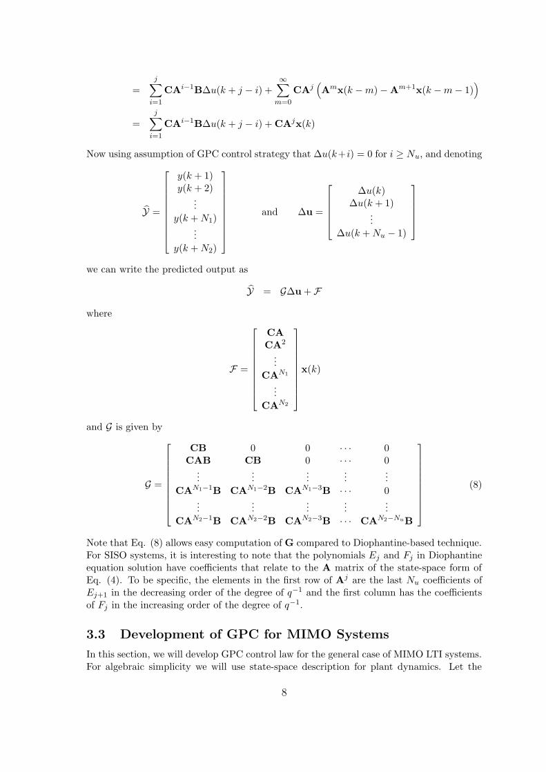
u(t)
y(t)
t-1 t t+1 t+j t+N
N
u(t+j|t)
y(t+j|t)^
... ...
Figure 1: MPC Strategy
2 GPC Control Paradigm
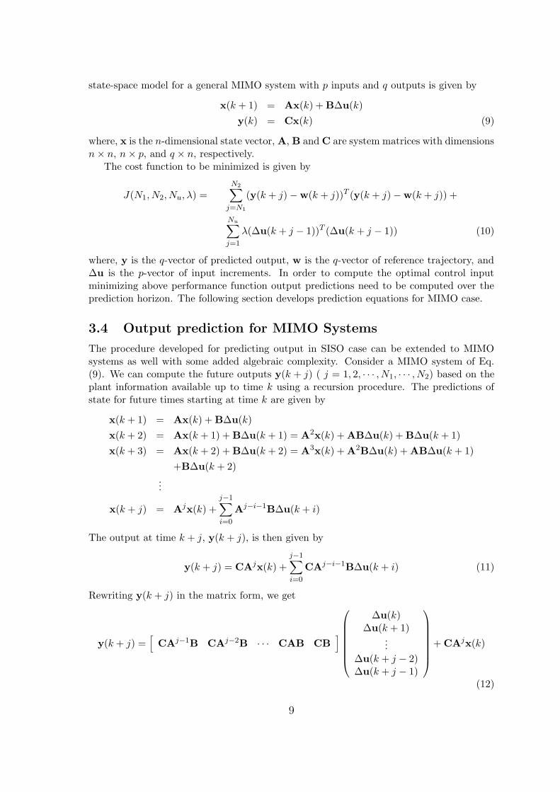
GPC is the most generalized form of MPC. Among all different types of MPC schemes, GPChas maximum design freedom available for choosing design parameters. MPC design hasseveral algorithms leading to different control schemes but all design schemes essentially usethe same design paradigm. There are three basic elements of MPC: the prediction model,the cost function, and the control law. Every MPC uses some kind of plant model to predictfuture plant outputs over a pre-defined prediction horizon, Ny = N2 − N1, where, N1 andN2 represent lower and upper prediction horizons, respectively. The predicted outputs,y(t + k|t) (k = N1, . . . , N2) depend on the past inputs and outputs and on the futurecontrol signals u(t + k|t), k = 1, 2, . . . , Nu, where Nu represents a control horizon. Aset of future control signals is calculated by optimizing a suitable performance index soas to keep the plant output as close to the reference trajectory w(t + k) as possible. Theperformance index is typically a quadratic function of the predicted tracking error andcontrol increments. The optimization is performed at each time step and the first elementof the optimized control sequence is sent to the plant. The whole process is repeated againat the next time step after “receding” the prediction horizon by one time-step. Because ofthis receding horizon feature of this control scheme it is sometimes referred to as RecedingHorizon Control as well. The MPC control strategy is illustrated in Figure 1. Figure showsthe predicted output based on plant model and predicted optimal control sequence basedon predicted future error. In the figure, the control horizon Nu is shown to be same asthe prediction horizon Ny, which is not necessary. In case of GPC, all design parameters,N1, N2, Nu, and λ ( control penalty in cost function) can be changed unlike other MPCschemes where one or more of these parameters are fixed. From this point on in the paperour focus will be on GPC control strategy unless otherwise mentioned. The control systemblock diagram for GPC is shown in Figure 2.
3 GPC Control of SISO Systems
Consider a discrete-time model of the single-input single-output (SISO) system describedusing a backward shift operator (q−1) as,
A(q−1)y(k) = q−dB(q−1)u(k − 1) + C(q−1)ξ(k)
∆(1)
3
Plant
Model (predictor)
Optimizer
Reference Trajectory
Predicted outputs
Cost function Constraints
Error input output
Figure 2: MPC block diagram
where u(k) and y(k) are the control and output sequences of the plant and ξ(k) is anuncorrelated random sequence. A, B, and C are the polynomials in the backward shiftoperator q−1:
A(q−1) = 1 + a1q−1 + a2q
−2 + · · · + anaq−na
B(q−1) = b0 + b1q−1 + b2q
−2 + · · · + bnbq−nb
C(q−1) = 1 + c1q−1 + c2q
−2 + · · · + cncq−nc
where d is the dead time of the system. ∆ is the difference operator 1 − q−1. This modelis known as a Controlled Auto-Regressive Integrating Moving Average (CARIMA) model.For simplicity in the development, without loss of generality, C(q−1) is chosen to be 1. Theplant (1) is then given by:
A(q−1)y(k) = q−dB(q−1)u(k − 1) +ξ(k)
∆(2)
The basic cost function used in GPC has the form
J(N1, N2, Nu, λ) =N2∑
j=N1
[y(k + j) − w(k + j)]2 +Nu∑
j=1
λ(j)[∆u(k + j − 1)]2 (3)
where, y(k + j) is an optimum j-step ahead prediction of the system output up to timek, w(k + j), j = 1, 2, . . . is a future set-point or reference sequence. N1 is the minimumprediction horizon, N2 is the maximum prediction horizon, Nu is the control horizon andλ(k) is a control-weighting sequence. As seen in Eq. (3), the cost function is quadraticand penalizes future tracking errors over prediction horizon and control energy over controlhorizon. It is assumed that the control increments after control horizon are zero. The basicidea is to compute the optimal future control sequence, u∗(k) = [u(k), u(k + 1), . . .], suchthat the cost function J(N1, N2, Nu, λ) is minimized. The control designer has to selectthe tuning parameters, N1, N2, Nu, and λ, to meet certain stability and performanceobjectives. Once u∗(k) is computed, only the first element of the sequence is used and thewhole process is repeated at next time step.
3.1 Prediction of future outputs
In order to compute the cost function, which consists of future tracking errors, we needto compute the future outputs, y(k + j) (N1 ≤ j ≤ N2), using the best available plant
4
model (2). In case of SISO systems, these predictions can be easily computed using theDiophantine equation [9]. The development of prediction equations for SISO case usingDiophantine approach is detailed in the Appendix 3.1. The prediction equations obtainedin section 3.1 using Diophantine approach are very cumbersome to use and are not easilyextendable to MIMO case. This motivates the development of state-space based formulationof prediction equations and control law.
3.2 State-space formulation of prediction equations
Consider a state-space description of the plant (Eq. 1) given as:
x(k + 1) = Ax(k) + B∆u(k) + Bξξ(k) (4)
y(k) = Cx(k) + ξ(k)
The reason for using the state-space form of the system with ∆u(k) as input is that thealgebraic complexity in the derivation of GPC control law reduces significantly in this form.The transformation of system equations with u(k) input to this form is given in detail inthe appendix. In Eq. (4), the dimension of state vector is n = max(na + 1, nb + d + 1, nc),and matrices A, B, Bξ, and C are given by
A =
−a1 1 0 · · · 0−a2 0 1 · · · 0
......
.... . .
...−ad+1 0 0 · · · 0
......
......
...−an 0 0 · · · 0
......
......
...−ana+1 0 0 · · · 0
B =
00...b0...
bn−d−1...
bnb−d−1
Bξ =
c1 − a1
c2 − a2...
cd+1 − ad+1...
cn − an
...cnc − anc
C =[
1 0 · · · 0 · · · 0 · · ·]
where ai are the coefficients of polynomial A, which is given by
Note that, in matrix B, the d leading elements are zeros. The block diagram representationof CARIMA model is shown in Fig. 3. If d = 0, the CARIMA model representationbecomes that of Fig. 4. If in addition to d = 0, C(q−1) = 1, the CARIMA model takes theform of Fig. 5, For both cases of Figs. 4 and 5, we can get the corresponding state-space
5
…… ……
∆u(k)
)(kξ
y(k)
)(1 kxn+ )(3 kx
∆u(k)
)(1 kx
∆u(k
)(2 kx
∆u(k)
q-1 q-1
bn-d-1 c1 c2 cn
1~a− 2
~a− na~−1~
+− naa
……
……
……
……
…… ……
)(2 kxd+
b0 cd+1
1~
+− da
……
……
……
Figure 3: The CARIMA model
∆u(k)
)(kξ
y(k)
)(1 kxna+
x (k)
)(1 kxn+
∆u(k)
)(3 kx
∆u(k)
)(1 kx
∆u(k
)(2 kx
∆u(k)
q-1
b0
q-1 q-1 q-1
bn-1 b1 c1 c2 cn
1~a− 2
~a− na~− 1~
+− naa
……
…… ……
……
…… ……
…… ……
Figure 4: The CARIMA model with d = 0
model.As mentioned previously, since the noise and disturbances in future are not known apriori
for prediction of future outputs only deterministic part of the plant model is consideredin the following development. The deterministic part of plant dynamics in polynomialdescription is given by
A(q−1)∆y(k) = B(q−1)∆u(k − 1) (6)
Let the corresponding state-space model be
x(k + 1) = Ax(k) + B∆u(k) (7)
y(k) = Cx(k)
Using the z-transform, we can obtain the z-domain transfer function H(z) as follows:
H(z) = C(zI − A)−1B
=C(I − A
z)−1B
z
6
∆u(k)
)(kξ
y(k)
)(1 kxna+
x (k)
)(1 kxn+
∆u(k)
)(3 kx
∆u(k)
)(1 kx
∆u(k
)(2 kx
∆u(k)
q-1
b0
q-1 q-1 q-1
bn-1 b1
1~a− 2
~a− na~− 1~
+− naa
……
…… ……
……
…… ……
…… ……
Figure 5: The CARIMA model with d = 0 and C(q−1) = 1
=C
z
(I +
A
z+
A2
z2+
A3
z3+ · · ·
)B
=CB
z+
CAB
z2+
CA2B
z3+ · · ·
By taking the inverse z-transform of the above equation, we get:
A general term y(k + j) (j = 1, 2, · · · , N2) in the above equation can be written as
y(k + j) =∞∑
i=1
CAi−1B∆u(k + j − i)
=j∑
i=1
CAi−1B∆u(k + j − i) +∞∑
i=j+1
CAi−1B∆u(k + j − i)
=j∑
i=1
CAi−1B∆u(k + j − i) +∞∑
m=0
CAm+jB∆u(k − m − 1)
=j∑
i=1
CAi−1B∆u(k + j − i) +∞∑
m=0
CAm+j (x(k − m) − Ax(k − m − 1))
7
=j∑
i=1
CAi−1B∆u(k + j − i) +∞∑
m=0
CAj(Amx(k − m) − Am+1x(k − m − 1)
)
=j∑
i=1
CAi−1B∆u(k + j − i) + CAjx(k)
Now using assumption of GPC control strategy that ∆u(k+i) = 0 for i ≥ Nu, and denoting
Y =
y(k + 1)y(k + 2)
...y(k + N1)
...y(k + N2)
and ∆u =
∆u(k)∆u(k + 1)
...∆u(k + Nu − 1)
we can write the predicted output as
Y = G∆u + F
where
F =
CACA2
...
CAN1
...
CAN2
x(k)
and G is given by
G =
CB 0 0 · · · 0CAB CB 0 · · · 0
......
......
...
CAN1−1B CAN1−2B CAN1−3B · · · 0...
......
......
CAN2−1B CAN2−2B CAN2−3B · · · CAN2−NuB
(8)
Note that Eq. (8) allows easy computation of G compared to Diophantine-based technique.For SISO systems, it is interesting to note that the polynomials Ej and Fj in Diophantineequation solution have coefficients that relate to the A matrix of the state-space form ofEq. (4). To be specific, the elements in the first row of Aj are the last Nu coefficients ofEj+1 in the decreasing order of the degree of q−1 and the first column has the coefficientsof Fj in the increasing order of the degree of q−1.
3.3 Development of GPC for MIMO Systems
In this section, we will develop GPC control law for the general case of MIMO LTI systems.For algebraic simplicity we will use state-space description for plant dynamics. Let the
8
state-space model for a general MIMO system with p inputs and q outputs is given by
x(k + 1) = Ax(k) + B∆u(k)
y(k) = Cx(k) (9)
where, x is the n-dimensional state vector, A, B and C are system matrices with dimensionsn × n, n × p, and q × n, respectively.
The cost function to be minimized is given by
J(N1, N2, Nu, λ) =N2∑
j=N1
(y(k + j) − w(k + j))T (y(k + j) − w(k + j)) +
Nu∑
j=1
λ(∆u(k + j − 1))T (∆u(k + j − 1)) (10)
where, y is the q-vector of predicted output, w is the q-vector of reference trajectory, and∆u is the p-vector of input increments. In order to compute the optimal control inputminimizing above performance function output predictions need to be computed over theprediction horizon. The following section develops prediction equations for MIMO case.
3.4 Output prediction for MIMO Systems
The procedure developed for predicting output in SISO case can be extended to MIMOsystems as well with some added algebraic complexity. Consider a MIMO system of Eq.(9). We can compute the future outputs y(k + j) ( j = 1, 2, · · · , N1, · · · , N2) based on theplant information available up to time k using a recursion procedure. The predictions ofstate for future times starting at time k are given by
The output at time k + j, y(k + j), is then given by
y(k + j) = CAjx(k) +j−1∑
i=0
CAj−i−1B∆u(k + i) (11)
Rewriting y(k + j) in the matrix form, we get
y(k + j) =[
CAj−1B CAj−2B · · · CAB CB]
∆u(k)∆u(k + 1)
...∆u(k + j − 2)∆u(k + j − 1)
+ CAjx(k)
(12)
9
Let us define
y =
y(k + N1)...
y(k + N2)
=
y1(k + N1)y2(k + N1)
...yq(k + N1)
...y1(k + N2)y2(k + N2)
...yq(k + N2)
(N2−N1+1)q×1
(13)
and
∆u =
∆u(k)∆u(k + 1)
...∆u(k + Nu − 1)
=
∆u1(k)∆u2(k)
...∆up(k)
∆u1(k + 1)∆u2(k + 1)
...∆up(k + 1)
...∆u1(k + Nu − 1)∆u2(k + Nu − 1)
...∆up(k + Nu − 1)
Nup×1
(14)
Then predicted outputs are given in a compact form as
y =
CAN1−1B CAN1−2B CAN1−3B · · · 0...
......
. . ....
CAN2−1B CAN2−2B CAN2−3B · · · CAN2−NuB
︸ ︷︷ ︸G
∆u +
CAN1
...
CAN2
x(k)
︸ ︷︷ ︸f
y = G∆u + f (15)
Note that the form of G in MIMO case is same as that of SISO case (Eq. (8)) except theprediction horizon is from N1 to N2. The cost function of Eq. (10) can be rewritten in acompact form as
J(N1, N2, Nu, λ) = (y − w)T (y − w) + λ∆uT ∆u
= (G∆u + f − w)T (G∆u + f − w) + λ∆uT ∆u (16)
10
where, y, ∆u, G, and f are given by Eqs. (13)-(15), and w is given by
w =
w(k + N1)w(k + N1 + 1)
...w(k + N2)
=
w1(k + N1)w2(k + N1)
...wq(k + N1)
...w1(k + N2)w2(k + N2)
...wq(k + N2)
(17)
Rewriting the cost function as,
J =1
2∆uTH∆u + b∆u + f0 (18)
where
H = 2[GTG + λI]
b = 2[(f − w)TG]
f0 = (f − w)T (f − w)
and setting
∂J
∂∆u= 0
we obtain the optimal control input ∆u∗ as follows:
∆u∗ = −H−1bT = −(GTG + λI)−1[GT (f − w)] (19)
The actual control signal sent to the process is the first p elements of the vector ∆u∗.
4 Stability of GPC control law
One of the major drawbacks of GPC control law presented in Eq. (19) is that the closed-loop stability under this control law can not be guaranteed. However, this difficulty canbe overcome if the performance function in Eq. (10) used to obtain the control law can bemodified to include the penalty on the end-state of the system and GPC design parameterscan be chosen in a certain way.
The approach that is taken here to prove the stability of the GPC control law is to usethe stability properties of the corresponding LQR problem. So, the optimal control problemcan now be stated as follows:
For the LTI system
x(k + 1) = Ax(k) + B∆u(k) (20)
y(k) = Cx(k)
11
determine the optimal control law that minimizes the cost with the end-point state weight-ing
where, wx(k + N2) is the desired value of the state at the end of the prediction horizon,N1 = 1, N2 = Nu = N , Q ≥ 0 and λ(j) = λ > 0.
Since the stability properties of the system are independent of the reference input, wecan ignore the reference input (or equivalently assume to be zero), i.e., set wx(k +N2) = 0,and w(k + j) = 0, ∀j. Then, the cost function will be modified to
JN = xT (k + N)Qx(k + N)
+N∑
j=1
y(k + j)Ty(k + j) + λ∆u(k + j − 1)Tu(k + j − 1)
= xT (k + N)(Q + CTC)x(k + N)
+N−1∑
j=0
x(k + j)TCTCx(k + j) + λ∆u(k + j)T ∆u(k + j)
−xT (k)CTCx(k) (22)
4.1 GPC control law with end-point weighting
The GPC control law derived in Section 3.3 is no more optimal for the cost function inEq. (22) since this cost function now includes additional penalty on the end-state of theprediction horizon which was absent in the cost of Eq. (16). The GPC control law for thismodified cost is derived next.
The state evolution equation for the plant in Eq. (20) is given by
x(k + N) = ANx(k) +N−1∑
i=0
AN−i−1B∆u(k + i)
= ANx(k) +[
AN−1B AN−2B · · · B]
︸ ︷︷ ︸C
∆u(k)∆u(k + 1)
...∆u(k + N − 1)
︸ ︷︷ ︸∆u
= ANx(k) + C∆u (23)
Using Eqs. (23) and (15) the cost function in Eq. (22) can be re-written in more compactform as
JN =1
2∆uT
[H + 2C
TQC
]∆u +
[b + 2xT (k)(AN )TQC
]∆u + f0 + xT (k)(AN )TQANx(k)(24)
12
where,
H = 2[GTG + λI
]
b = 2fTG
f0 = fT f
Matrices G and f are as defined in Eq. (15) and f is given as
f =
CA1
CA2
...
CAN
︸ ︷︷ ︸L
x(k) = Lx(k)
Let the cost function in Eq. (24) be further simplified to
JN =1
2∆uTH∆u + b∆u + f0 (25)
where
H = 2[GTG + λI + C
TQC
]
b = 2xT (k)[LTG + (AN )TQC
]
f0 = xT (k)(LT L + (AN )TQAN
)x(k)
Now the optimal control ∆u∗ can be obtained by setting the gradient of Eq. (25) to zerowith respect to ∆u. That is,
∂J
∂∆u= 0 ⇒
∆u∗ = −H−1
bT
= −(GTG + λI + C
TQC
)−1 (GT L + C
TQAN
)x(k)
= −Kx(k) (26)
The following lemmas give the stability result for the corresponding LQR problem whichwill be used in proving the stability of GPC control law and the connection between GPCand LQR control laws.
Lemma 1 For the system (20) the optimal control law minimizing the LQ performanceindex (22) is given by
∆u∗(k) = −K(k)x(k) (27)
where, gain K(k) is given by
K(k + j) = [BT P (k + j + 1)B + λI]−1BT P (k + j + 1)A (28)
and P is the solution of the following Riccati Difference Equation (RDE)
P (k+j) = AT P (k+j+1)A−AT P (k+j+1)B[BT P (k+j+1)B+λI]−1BT P (k+j+1)A+CTC
(29)with the boundary condition
P (k + N) = Q + CTC (30)
13
Proof 1 Proof is given in the appendix.
Lemma 2 For the system shown in Eq. (20) and the performance function given in Eq.(22), the GPC control law given by Eq. (26) is same as the LQR control law (Eq. C.26)evaluated at the same time instant
Proof 2 Proof is given in the appendix.
4.2 Stability result
The RDE in Eq. (C.28) can be re-written by reversing the time index by defining
Pm := P (k + N − m), where m = 0, 1, 2, · · · , N − 1
Then, the RDE in the forward form becomes
Pm+1 = AT PmA − AT PmB(BT PmB + λI)−1BT PmA + CTC (31)
with initial condition P0 = Q + CTC.Now, if we consider the steady-state solution for the infinite horizon problem, i.e., let
N → ∞ and let Pm = Pm+1 = P =constant as m → ∞, then, Eq. (31) becomes theAlgebraic Riccati Equation (ARE) in variable P :
P = AT PA − AT PB(BT PB + λI)−1BT PA + CTC (32)
The following lemma is state without proof which gives the conditions under which thematrix P has the stabilizing property.
Lemma 3 If the system (A, B, C) is stabilizable and detectable, and P0 0, then thematrix sequence, Pm∞m=0, generated by the RDE (Eq. (31)) has a unique limit P whichstabilizes the system and satisfies the Algebraic Riccati Equation (ARE) (Eq. (32)).
Theorem 1 If the system given by Eq. (20) is stabilizable and detectable, P0 P1, Q 0,λ > 0, N1 = 1, and N2 = Nu = N , then the GPC control law of Eq. (26) stabilizes thesystem.
Proof 3 In order to show stability of GPC control law, it suffices to show that the feedbackgain K used in Eq. (26) is stabilizing. From Lemma 2, this is equivalent to showing thatthe corresponding LQR gain in Eq. (C.26) is stabilizing. Note that as long as the GPCparameters (N1, N2, Nu, and λ) are fixed the GPC control is equivalent to a constant-gainstate feedback.
Rewrite the RDE (Eq. (31)) as a set of two equations:
Pm = AT PmA−AT PmB(BT PmB + λI)−1BT PmA + Q(m)
Q(m) : = CTC + (Pm − Pm+1) (33)
where, first of Eq. (33) is nothing but an ARE for a given m. They are also referred toas Fake Algebraic Riccati Equations (FARE) in the literature. Now, by Lemma 3 if thesystem is stabilizable and detectable and Pm −Pm+1 0 , Pm will stabilize the system, i.e.,A = A−B(BT PmB+λI)−1BT PmA will have all of its eigenvalues strictly within the unitcircle. Next, we will use the monotonicity properties of the RDE and the property of FARE
14
to show the stability of GPC.Consider matrix Pk defined as follows
Pk = Pk−1 − Pk
Then, from the result (Fact 5.2.1) on Page 95 of [22], Pk satisfies the RDE
Pk+1 = AT
k PkAk − AT
k PkB(BT PkB + λk)−1BT PkAk
where
Ak = A−B(BT PkB + λI)−1BT PkA
Q(k) = CTC−CTC = 0
λk = BT PkB + λI 0
Now, if
P1 = P0 − P1 0
by the property of the solution of the RDE,
PN = PN−1 − PN 0.
Then, from first of Eq. (33), PN−1 stabilizes the system. Since, PN−1 = P (k + 1), theLQR controller gain K(k) in Eq. (C.26) stabilizes the system. Now, from Lemma 2, GPCcontroller gain K in (Eq. (26)) stabilizes the system
4.3 GPC control law for non-zero reference trajectory
In the case when the desired trajectory is non-zero time varying the GPC control law (Eq.(26)) takes slightly different form to account for the tracking error. Consider the LTI system
In most real life situations it is safe to assume that the desired output trajectory is givento the control designer. However, the control law computation (Eq. 36) requires that thedesired state trajectories are known. This section gives the procedure for computing thedesired state trajectories given the desired output trajectories for a general case.
Consider MIMO LTI system given by the following state-space description
x(k + 1) = Ax(k) + B∆u(k). (37)
Let w(k + N2) denote the desired output trajectory that needs to be tracked by the sys-tem and let wx(k + N2) denote the corresponding trajectories for the desired state. Then,wx(k + N2) must satisfy the following conditions:
w(k + N2) = Cwx(k + N2) (38)
(A − I)wx(k + N2) = 0 (39)
The first condition (Eq. 38) is a direct consequence of output equation. The second condi-tion (Eq. 39) is derived next.
One consideration in tracking problem is that the choice of wx(k + N2) should be con-sistent with the zero steady-state output tracking error. Consider the GPC control lawwith tracking error feedback:
∆u∗(k) = −Ke(k) (40)
where
e(k) = x(k) − wx(k)
The closed-loop error dynamics for the system given by Eq. (37) with control law (40) isgiven by
e(k + 1) = x(k + 1) − wx(k + 1)
= Ax(k) + B∆u∗(k) − wx(k + 1)
= (A − BK)e(k) + Awx(k) − wx(k + 1).
16
At steady-state, for zero tracking error we need
e(k + 1) = e(k) = 0, and wx(k) = wx(k + 1).
Then, to satisfy the end-point constraint of zero tracking error, we need
(A − I)wx(k + N2) = 0.
Combining the conditions of Eqs. (38) and (39), we get
[A − I
C
]wx(k + N2) =
[0
w(k + N2)
](41)
Note that Eq. (41) typically represents under-determined system of equations as matrix onthe left hand side is not generally invertible. In such as case, a least square solution can beobtained for the desired state trajectories as
wx(k + N2) =
([A − I
C
])† [0
w(k + N2)
](42)
where (·)† denotes pseudo-inverse of (·).
4.4.1 Special Case: System with redundant actuators
For the system which has more inputs than outputs, i.e. p > q, the transformation of thesystem with u(k) as input to the form which has ∆u(k) as input, the detectability may belost. To see this, consider the matrix
[λI − A
C
](43)
where A and C are defined as in Eq. (B.16). When λ = 1, rank of (λI − A) is less thann− p. The rank of C can at the most be q. So, the matrix in Eq. (43) must have rank lessthan n, which is not a full column rank. That is, the detectability is lost. However, thisproblem can be addressed as follows:
Consider a system with ∆u(k) as input and let the number of inputs be greater thanthe number of outputs, i.e., p > q.
x(k + 1) = Ax(k) + B∆u(k)
y(k) = Cx(k) (44)
Now consider a modified output y(k) such that
y(k) = Cx(k) (45)
where
y(k) =
[y(k)
u(k − 1)
], C =
[C
0p×(n−p) Ip×p
](46)
17
It can be verified that with respect to this new output the system is detectable. Thus, themodified system now takes the form:
x(k + 1) = Ax(k) + B∆u(k) (47)
y(k) = Cx(k) (48)
which is stabilizable and detectable. For this new system, let the cost function be modifiedas follows:
J = xT (k + N)Qx(k + N) +N∑
j=1
yT (k + j)Qy(k + j) +N∑
j=1
λ∆u(k + j − 1) (49)
where
Q =
[Iq×q
0p×p
](50)
Now, it can be seen that minimizing the cost function given by Eq. (49) for the systemgiven by Eq. (47) is same as minimizing the original cost function (Eq. 22) for originalsystem (Eq. 44). The advantage in dealing with transformed system is that it satisfies theconditions of stability theorem and therefore allows computation of GPC control law.
Now, to show that the stability proof still holds consider the following:We have already shown that the modified cost function is essentially same as the original
cost function. Now it remains to show that the Riccati equations used in Lemma 1 withappropriate boundary condition do not change as a result of transformed system. Theequations in Lemma 1 for the modified system can be rewritten as:
∆u∗(k) = −K(k)x(k)
where
K(k + j) = [BT P (k + j + 1)B + λI]−1BT P (k + j + 1)A
P (k + j) = AT P (k + j + 1)[A − BK(k + j)] + CTQC
with
P (k + N) = Q + CTQC.
By direct substitution, it can be easily verified that
CTQC = CTC.
This essentially proves that the GPC control law derived for the transformed system stabi-lizes the original system.
18
5 Reconfigurable control
In this section, we will extend the stability result obtained in previous section to the case ofreconfigurable control architecture. We present a reconfigurable control scheme wherein thesystem has some redundancy in control actuators and in the event of actuator failures, likesaturation for example, the system can reconfigure itself to re-allocate the control signal toother set of actuators.
Consider a strictly proper stabilizable and detectable MIMO LTI system from Eq. (9)with p inputs and q outputs.
x(k + 1) = Ax(k) + B∆u(k) (51)
y(k) = Cx(k)
Let us suppose that the system has some redundancy in actuators, i. e., p ≥ q and some ofthe p inputs can control more than one outputs. The reconfiguration problem is defined asfollows. If one or more of the p actuators saturate (i.e., become “inactive”) how to re-allocatethe control signal to actuators which are still “active” such that the lost degrees of freedomdue to saturation in controlling certain outputs are regained via re-allocation. Moreover,to ensure that the overall stability of the system is maintained under such reconfiguration.Before reconfiguration scheme is presented and stability of such scheme is established somedefinitions are in order.
5.1 Definitions
Definition 1 Reconfiguration matrix: Any q × p matrix with binary entries (0 or 1) iscalled as Reconfiguration Matrix, Qrc, and is used to set the control priorities for eachactuator.
Qrc is used to select which actuator is used to control a certain output. The size of the Qrc
matrix is q (number of outputs) by p (number of inputs). Each element of Qrc is either 1or 0 indicating weather a particular actuator is allowed to control a specific output or not.For example, let us take a 5-input 2-output system. An example Qrc matrix could be
Qrc =
[0 1 0 0 00 0 1 1 0
](52)
In this example of Qrc, the first output can be controlled only by the second input, and thesecond output can be controlled by both the third and fourth inputs.
This matrix is then used to “reconfigure” the H matrix (where H is the transfer functionmatrix of system in Eq. (51)) as follows which causes the reconfiguration. Reconfigured Hmatrix is denoted by Hrc and is given by
Hrc = Qrc ⊗ H (53)
where, ⊗ indicates the outer product. This outer product effectively modifies the B andthe c matrix of the system to account for reconfiguration.
Definition 2 Let Q be the set of all allowable Qrcs such that the outer product in Eq. (53)produces a set of reconfigured stabilizable and detectable systems.
19
That is,
Q =Qi
rc | (A, Bi, Ci) is stabilizable and detectable ∀i
(54)
where, Bi is the reconfigured B matrix and Ci is the reconfigured C matrix as a result ofouter product of Qi
rc with G.
Definition 3 The matrix designed to prioritize the order of the actuators in which theyare used in the event of saturation failure is called as Reconfiguration Order Matrix.
The design of the reconfiguration matrix Qrc is based on the criteria designed suitably basedon the application, for example one of the criteria could be the saturation of the actuators.The order in which the redundant actuators are used is based on the reconfiguration ordermatrix, Qro. For example, for the Qrc defined in Eq. (52) a reconfiguration order matrixcould be
Qro =
[4 1 2 2 34 3 1 1 2
](55)
This Qro matrix informs the reconfiguration algorithm to use the second input to controlthe first output until it saturates followed by actuators 3 and 4 until they saturate followedby actuators 5 and then 1. Similar logic is used for the second output. Each time thecontrol law is evaluated, the first actuators are used to calculate the control input. Theinput is tested for saturation, if it is saturated, the Qrc matrix is set to the next actuator(or set of actuators). This process is repeated until there is no change in the Qrc matrix orthere are no more free actuators left. Then, the resulting control is sent to the plant. Thisprocess is repeated at each cycle. The repeating of this process ensures that the reverseorder of actuators is used as the actuators unsaturate.
5.2 Stability under reconfigurable control
The stability of the reconfigurable control architecture described above will be establishedin two steps. In the first step, it will be shown that the set of plants obtained afterreconfiguration is stabilized by the GPC control law of Eq. (26). Then, in the secondstep, it will be shown that the system remains stable during the switching of the controllaw under reconfiguration. The stability of the reconfigured system is established by thefollowing theorem.
Theorem 2 All systems resulting from reconfiguration of system given by Eq. (51) due toreconfiguration matrix Qrc are stabilized by the control law of Eq. (26) iff Qrc belongs tothe set Q.
Proof 4 Proof of this theorem is the direct consequence of Definition 2 and Theorem 1.
Note that the control law of Eq. (26) stabilizes the original system (Eq. (51)) as wellaccording to Theorem 1. Having established that both systems - system before reconfigu-ration and the system after reconfiguration - are stabilized by the control law of Eq. (26),to complete the stability argument we need to show that the stability is retained during theprocess of reconfiguration. For that, let the system after reconfiguration is described by
x(k + 1) = Ax(k) + B∆u(k) (56)
y(k) = Cx(k)
20
Let us suppose that the system (51) is under closed-loop control with control law givenby Eq. (26). Suppose the system has actuator saturation at time instant k = r and isreconfigured by matrix Qrc ∈ Q to yield the system of Eq. (56). That means, the dynamicsof the system (51) starting at say initial time k = 0 is governed by the dynamics of system(56) after reconfiguration (i.e., for ∀ k ≥ r). Since the GPC control of Eq. (26) is stabilizingfor system (51), x(r) is bounded. Let x(r) be the initial condition for the system (56) attime instant k = r. Since x(r) is related to x(r) by some similarity transformation, x(r)is also bounded. Now, for time k > r, system evolves according the dynamics of Eq. (56).From Theorem 2, the system (56) is also stabilized by the control law of Eq. (26), i.e., x(k)remains bounded for all r < k ≤ ∞. Thus we have shown that the system remains stablefor all 0 ≤ k ≤ ∞ under control law of Eq. (26)
6 Numerical Example
In this section, a numerical example is given to demonstrate stable reconfiguration capabilityof the GPC control methodology presented in Section 5 using a short-period approximationmodel of an aircraft. Two different cases of reconfiguration are presented where each casecan be considered to represent a different type of actuator limitation and/or failure.
The short-period approximation model of an aircraft considered is:
x(t) =
[0 −1.3677
1.0000 −1.5087
]x(t) +
[−0.0665 −0.0029 −0.0029−0.0862 −0.0043 −0.0043
]u(t)
y(t) =[
0 0.2500]x(t)
where the inputs are elevator deflection, left aileron deflection, and right aileron deflection.The eigenvalues of the open-loop system are −0.7543 ± 0.8937i. The maneuver underconsideration is the step change in the pitch-rate. The initial actuator configuration is suchthat only the desirable input is the elevator input to accomplish this task. The left andright ailerons are considered as redundant actuators and are to be used if elevator fails.For demonstrating reconfiguration capability two different cases are considered: Case (i)system reaches the steady-state condition and elevator fails to hold its position and elevatorinput suddenly drops to zero; and Case (ii) before system reaches to target output elevatorfreezes in its position and some constant input is acting on the system but not adequate toreach the desired position. These two cases are chosen as they represent two quite differentdynamic characteristics. In the first case the redundant actuators (both ailerons) have tocompensate for no elevator input and try to return system to desired steady-state conditionwhereas in the second case the ailerons have to make-up for the inadequate control inputto reach to the desired steady-state. Given below are reconfiguration results based on themethodology presented in Section 5.Reconfiguration strategy and GPC control law design: For both cases, the stepsinvolved in the control law design are same and are given below. The reconfiguration matrixQrc has its initial settings as:
Qrc =[
1 0 0],
21
The outer product of Qrc with the system transfer matrix yields the following system
x(t) =
[0 −1.3677
1.0000 −1.5087
]x(t) +
[0.25000.2758
]u(t)
y(t) =[−0.0128 −0.0665
]x(t) (57)
The discretization of the system of Eq. (57) with sampling time, T = 0.05s, we get
x(k + 1) =
[0.9983 −0.06580.0481 0.9257
]x(k) +
[0.01200.0136
]u(k)
y(k) =[−0.0128 −0.0665
]x(k) (58)
Now, using the transformation given in the Appendix B we can transform the system to anew system which has ∆u(k) as input as follows:
x(k + 1) =
0.9983 −0.0658 0.01200.0481 0.9257 0.0136
0 0 1.0000
x(k) +
0.01200.01361.0000
∆u(k)
y(k) =[−0.0128 −0.0665 0
]x(k) (59)
It can be verify that the system in Eq. (59) is stabilizable but not detectable. In orderto satisfy the conditions of the stability theorem given in Section 4, we define a fictitiousoutput and augment the output matrix to be
Caug =
[−0.0128 −0.0665 0
0 0 1
](60)
With this newly defined C matrix, the system is stabilizable and detectable. Now, choosingthe GPC design parameters as: N1 = 1, N2 = Nu = 5, λ = 0.1, and end-point weightingmatrix Q = diag150 800 1 we can obtain a stabilizing control law. The Riccati solutionsP0 and P1 for these set of design parameters are given below.
This system again is not detectable and one can define new fictitious output as before anddefine a new C matrix as
Caug =
−0.0000 0.0313 0 00 0 1.0000 00 0 0 1.0000
(65)
The modified system with this new C matrix is again controllable and observable. Now ifwe define the new GPC parameters to be N1 = 1, N2 = Nu = 5, λ = 0.1, and the end-pointweighting matrix as Q = diag130 200 1 1, we obtain the following Riccati solutionswhich satisfy the stability condition of Theorem 1 as shown below:
Thus the conditions in the Theorem 1 are satisfied and the GPC control law (Eq. (26))stabilizes the system.
23
Case (i): Consider the first of the two cases mentioned above. In this case, it is assumedthat after system output (pitch rate) reaches its steady-state value of 1.15 deg/sec theelevator input abruptly goes to zero (at t = 2 secs) (potentially this could be a result ofpossible failure) and system is reconfigured using Eq. (6).
Figure 7 shows the system response before and after reconfiguration. It can be seenthat the system reaches a zero steady-state error within 2 seconds and when elevator inputabruptly goes to zero at t = 2 secs, the output starts drifting from the desired value. Att = 2 sec reconfiguration takes place and ailerons take over and bring back the output backto the desired value rendering zero steady-state error. The input time histories are given inFig. 6. As shown in the figure, the elevator deflection has abruptly dropped to zero afterreaching an approximate steady-state value of −1.8 deg and at the same instant aileronstake over and bring the output back to the desired value. The ailerons reach the steadydeflection of about −19 deg. The cost and tracking error plots are given in Figs. 8 and 9,respectively.
0 2 4 6 8 10 12−20
−15
−10
−5
0
5
Time (sec)
Inpu
t (de
g)
ElevatorLeft AileronRight AileronReconfiguration
Figure 6: The GPC control law
0 2 4 6 8 10 120
0.2
0.4
0.6
0.8
1
1.2
1.4
Time (sec)
Pitc
h ra
te (
deg/
sec)
Reference outputPlant output
Reconfiguration
Figure 7: The Plant Output
24
10−2
10−1
100
101
102
10−8
10−6
10−4
10−2
100
102
104
Time (sec)
Cos
t
Reconfiguration
Figure 8: The Cost Function
0 2 4 6 8 10 12−1.2
−1
−0.8
−0.6
−0.4
−0.2
0
0.2
Time (sec)
Pitc
h ra
te e
rror
(de
g/se
c) Reconfiguration
Figure 9: The Plant Output Error
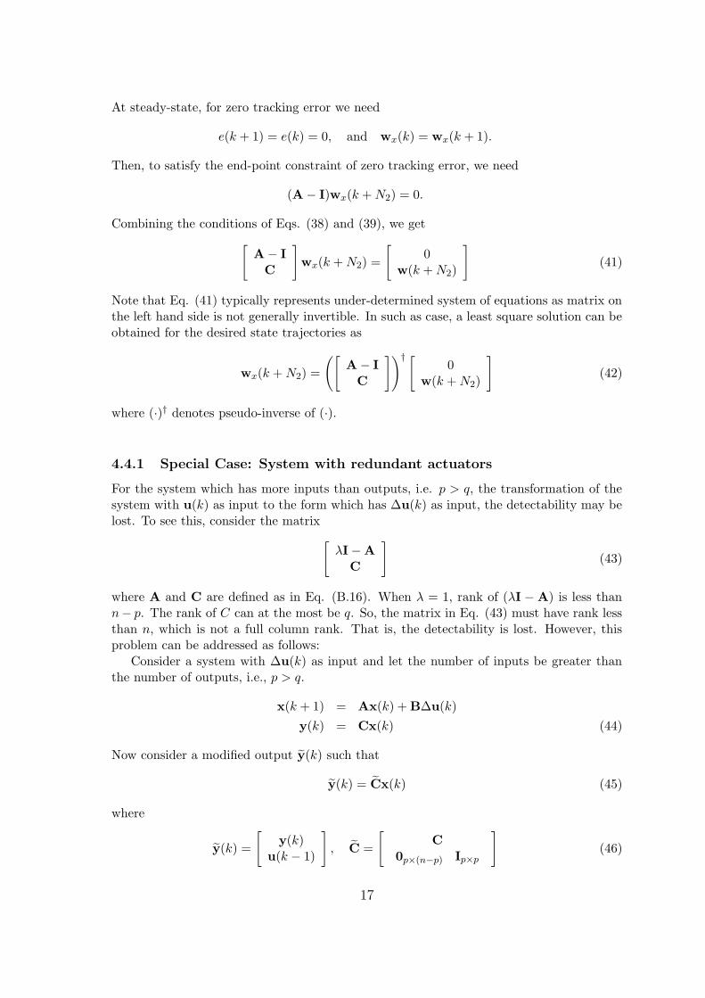
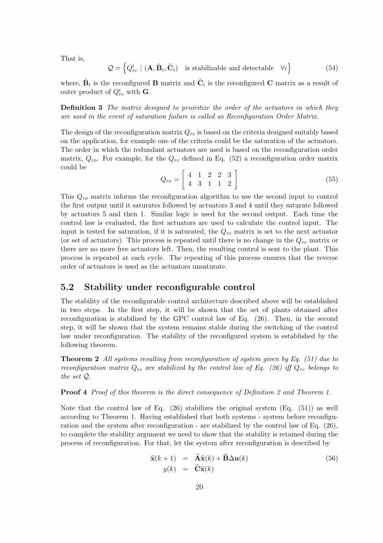
Case (ii): In the second case, it is assumed that the elevator input freezes to somenonzero constant −6 deg before the system output (pitch rate) reaches its desired value(5.73 deg/sec). The simulation results for this case are shown in Figures 10-13. As shownin Fig. 10, the elevator input freezes approximately at −6 deg when the system output hasreached only 90% of its final value. At this time ailerons take over as a result of reconfig-uration and ailerons deflection reaches a steady-state value of approximately −21 deg aspitch rate reaches to desired value of 5.73 deg/sec. As seen in Fig. 11, overall trackingperformance is very satisfactory without steady-state error. The performance function andtracking error time history is shown in Figs. 12 and 13, respectively.
7 Concluding Remarks
This paper presented a comprehensive development of the basic GPC control architectureand derivation of control law for SISO as well as MIMO systems. For SISO systems, both
25
0 2 4 6 8 10 12−30
−25
−20
−15
−10
−5
0
5
Time (sec)
Inpu
t (de
g)
ElevatorLeft AileronRight Aileron
Reconfiguration
Figure 10: The GPC control law
0 2 4 6 8 10 120
1
2
3
4
5
6
7
Time (sec)
Pitc
h ra
te (
deg/
sec)
Reference outputPlant output
Reconfiguration
Figure 11: The Plant Output
z-domain (i.e., polynomial-based) as well as state-space based control law developmentwas given. Stability of GPC based on end-point constraints was presented as a basis forestablishing stability of a novel reconfigurable GPC control architecture. The stabilityconditions for reconfiguration scheme were presented. A numerical example consistingof longitudinal control of aircraft was presented to demonstrate the effectiveness of theproposed reconfiguration methodology.
8 Acknowledgements
The second and third author acknowledge the financial support from NASA Ames ResearchCenter, Moffett Field, CA, through Grant No. NAG2-1471 under the direction of Dr.Michael R. Lowry, Computational Sciences Division.
26
10−2
10−1
100
101
102
100
101
102
103
Time (sec)
Cos
t
Reconfiguation
Figure 12: The Cost Function
0 2 4 6 8 10 12−6
−5
−4
−3
−2
−1
0
1
Time (sec)
Pitc
h ra
te e
rror
(de
g/se
c) Reconfiguration
Figure 13: The Plant Output Error
References
[1] J. Richalet, A. Rault, J.L. Testud, and J. Papon: ‘Algorithmic COntrol of IndustrialProcesses’. In 4th IFAC symposium on Identification and System Parameter Estima-tion. Tbilisi URSS, 1976.
[2] J. Richalet, A. Rault, J.L. Testud, and J. Papon: ‘Model Predictive Heuristic Control:Application to Industrial Processes’, Automatica, 14(2):413-428, 1978.
[3] A. I. Propoi: ‘Use of LP Methods for Synthesizing Sampled-Data Automatic Systems’,Automn Remote COntrol, 24, 1963.
[4] V. Peterka: ‘Predictor-Based Self-Tuning Control,’ Automatica, 20(1):39-50, 1984.
[5] B. E. Ydstie: ‘Extended Horizon Adaptive Control’, IN Proc. 9th IFAC WorldCongress, Budapest, Hungary, 1984.
[6] C. Greco, G. Menga, E. Mosca, and G. Zappa: ‘Performance Improvement of Self-tuning COntrollers by Multi-Step Horizons: the MUSMAR approach’, Automatica,20:681-700, 1984.
27
[7] J. M. Lemos and E. Mosca: ‘A Multipredictor-based LQ Self-tuning Controller’, InIFAC Symposium on Identification and System Parameter Estimation, York, UK, 137-141, 1985.
[8] J. Richalet, S. Abu el Ata-Doss, C. Arber, H.B. Kuntze, A, Jacubash, and W. Schill:‘ Predictive Functional Control: Application to Fast and Accurate Robots,’ In Proc.10th IFAC Congress, Munich, 1987.
[9] R. Soeterboek: ‘Predictive Control: A Unified Appraoch,’ Prentice Hall, 1992.
[10] M Morari: ‘Advances in Model-based Predictive COntrol’, Chapter in Model-basedPredictive Control: Multivaraible Control Technique of Choice in the 1990s?’, OxfordUniv. Press, 1994.
[12] D. W. Clarke and Scattolini: ‘Constrained Receding-horizon Predictive Control’, Proc.IEE, 138(4),:347-354, July 1991.
[13] E. Mosca, J. M. Lemos, and J. Zhang: ‘Stabilizing I/O Receding Horizon Control,’IEEE Conf. in Decision and Control, 1990.
[14] K.R. Muske and J. Rawlings: ‘Model Predictive Control with Linear Models’, AICHEJournal, 39:262-287, 1993.
[15] Ming Ding: ‘Neural Network-Based Predictive Control of Uncertain Systems,’ M.S.Thesis, Mechanical Engineering Dept., Kansas State University, 1998.
[16] D.W.Clarke, C.Mohtadi, and P.S.Tuffs: Generalized Predictive Control- Part I. TheBasic Algorithm, Automatica, 23(2), 1987.
[17] D.W.Clarke, C.Mohtadi, and P.S.Tuffs: Generalized Predictive Control- Part II. Ex-tensions and Interpretations, Automatica, 23(2), 1987.
[18] Properties of Generalized Predictive Control, D.W.Clarke, C.Mohtadi, Automatica,25(6),1989.
[19] R.R.Bitmead, M.Gevers, V.Wertz, and K.Ogata: Adaptive Optimal Control: TheThinking Man’s GPC, Prentice Hall, Englewood Cliffs, New Jersey, 07632, 1990.
[20] H.Demircioglu and D.W.Clarke: Generalized predictive control with end-point stateweighting, IEE Proceedings-D, Vol. 140, No.4, July 1993.
[21] C.L.Phillips and H.T.Nagle: Digital Control System Analysis and Design, Third Edi-tion, Prentice Hall, Saddle River, New Jersey 07458, 1995.
[23] K.Ogata: Discrete-Time Control Systems, Second Edition, Prentice Hall, EnglewoodCliffs, New Jersey, 07632, 1995.
[24] E.F.Camacho and C.Bordons: Model Predictive Control, Springer-Verlag London Lim-ited,1999.
[25] Jeffrey B.Burl: Linear Optimal Control: H∈ and H∞ Methods, Addison-Wesley, 1999.
[26] B.L.Stenvens and F.L.Lewis: Aircraft Control and Simulation, John Wiley and Sons,INC. 1992.
28
[27] R.A.Hess and Y.C.Jung: An Application of Generalized Predictive Control to Rotor-craft Terrain-Following Flight, IEEE Transaction on Systems, Man and Cybernetics,19(5), 1989.
[30] D.Q.Mayne, J.B.Rawlings, C.V.Rao, and P.O.Scokaert: Constrained Model PredictiveControl: Stability and Optimality, Automatica, 36, 789-814, 2000.
[31] J.A.Primbs and V.Nevistic: Feasibility and Stability of Constrained Finite RecedingHorizon Control, Automatica, 36(7), 956-971, 2000.
[32] J.A.Primbs and V.Nevistic: Constrained Finite Receding Horizon Linear QuadraticControl, Proceedings of 36th Conference on Decision and Control, 1997.
[33] A.Jadbabaie, J.Primbs, and J.Hauser: Unconstrained Receding Horizon Control withNo Terminal Cost, Proceedings of the American Control Conference, 2001.
29
Appendix
A Diophantine equation
The Diophantine equation offers a convenient way to obtain a division of two polynomialsand has the following form:
1 = Ej(q−1)A(q−1) + q−jFj(q
−1) (A.1)
where A(q−1) = ∆A(q−1). The degrees of polynomials Ej and Fj are j − 1 and na,respectively. This equation will be useful in writing predictions of future outputs. TheDiophantine equation has a unique solution, Ej and Fj , given A(q−1) and the predictioninterval j.
Consider Eq. (2) and multiply it by Ej∆qj to obtain
As the degree of polynomial Ej(q−1) = j − 1 the noise terms in Eq. (A.3) are all in the
future and therefore can be omitted from the prediction as any better prediction of noiseis not possible. The best prediction of y(k + j) is therefore given by
y(k + j) = Gj(q−1)∆u(k + j − d − 1) + Fj(q
−1)y(k) (A.4)
where, Gj(q−1) = Ej(q
−1)B(q−1). Since the degrees of Ej and Fj are j − 1 and na, the jth
prediction of output involves the past outputs: (y(k), y(k − 1), · · · , y(k − na)) and inputs(∆u(k + j − d − 1), ∆u(k + j − d − 2), · · · , ∆u(k − d − nb)). The polynomials Ej and Fj
obtained from Eq. (A.1) are given by
Ej(q−1) = ej,0 + ej,1q
−1 + · · · + ej,j−1q−(j−1)
Fj(q−1) = fj,0 + fj,1q
−1 + · · · + fj,naq−na
Now, the same Diophantine equation can be used to obtain Ej+1 and Fj+1, where
Fj+1(q−1) = fj+1,0 + fj+1,1q
−1 + · · · + fj+1,naq−na
and the polynomial Ej+1 is be given by
Ej+1(q−1) = Ej(q
−1) + ej+1,jq−j
with ej+1,j = fj,0. The polynomial Gj+1 can now be obtained recursively as follows
Gj+1 = Ej+1B = (Ej + fj,0q−j)B
= Gj + fj,0q−jB (A.5)
30
where
Gj(q−1) = gj,0 + gj,1q
−1 + gj,2q−2 + · · · (A.6)
From Eqs. (A.5) and (A.6), it can be seen that the first j coefficients of Gj+1 will beidentical to those of Gj and the remaining ones are given by
gj+1,j+i = gj,j+i + fj,0bi i = 0, · · · , nb
In the case when system has a dead time of d, the output of the system at any time instantk is the result of input applied to the system at time k − d. As a result, the horizons N1
and N2 should be chosen such that N2 ≥ N1 ≥ d + 1.Now consider the following set of j-step ahead optimal predictions for j = d+1, · · · , N2:
y(k + d + 1) = Gd+1∆u(k) + Fd+1y(k)
y(k + d + 2) = Gd+2∆u(k + 1) + Fd+2y(k)
...
y(k + N1) = GN1∆u(k + N1 − d − 1) + FN1
y(k)
...
y(k + N2) = GN2∆u(k + N2 − d − 1) + FN2
y(k)
which can be re-written as:
Y = G∆u + F(q−1)y(k) + G ′(q−1)∆u(k − 1) (A.7)
where
Y =
y(k + d + 1)y(k + d + 2)
...y(k + N1)
...y(k + N2)
∆u =
∆u(k)∆u(k + 1)
...∆u(k + Nu − 1)
G =
g0 0 0 · · · 0g1 g0 0 · · · 0...
......
......
gN1−d−1 gN1−d−2 gN1−d−3 · · · 0...
......
......
gN2−d−1 gN2−d−2 gN2−d−3 · · · gN2−Nu−d
G′(q−1) =
(Gd+1(q−1) − g0)q
(Gd+2(q−1) − g0 − g1q
−1)q2
...
(GN1−d−1(q−1) − g0 − g1q
−1 − · · · − gN1−d−1q−(N1−d−1))qN1−d
...
(GN2−d−1(q−1) − g0 − g1q
−1 − · · · − gN2−d−1q−(N2−d−1))qN2−d
31
and
F(q−1) =
Fd+1(q−1)
Fd+2(q−1)
...Fd+N1
(q−1)...
Fd+N2(q−1)
Thus, the predicted outputs over the prediction horizon are given by
y =
y(k + N1)y(k + N1 + 1)
...y(k + N2)
= G∆u + f (A.8)
where,
G =
gN1−d−1 gN1−d−2 · · · 0gN1−d gN1−d−1 · · · 0
......
. . ....
gN2−d−1 gN2−d−2 · · · gN2−Nu−d
and
f =
Fd+N1(q−1)
...Fd+N2
(q−1)
y(k)
+
(GN1−d−1(q−1) − g0 − g1q
−1 − · · · − gN1−d−1q−(N1−d−1))qN1−d
...
(GN2−d−1(q−1) − g0 − g1q
−1 − · · · − gN2−d−1q−(N2−d−1))qN2−d
∆u(k − 1)
A.1 Control law
Using Eq. (A.8), the cost function (Eq.(3)) can be written as
J(N1, N2, Nu, λ) = (G∆u + f − w)T (G∆u + f − w) + λ∆uT ∆u (A.9)
where
w =
w(t + d + N1)w(t + d + N1 + 1)
...w(t + d + N2)
Equation (A.9) can be re-written as
J(N1, N2, Nu, λ) =1
2∆uTH∆u + b∆u + f0 (A.10)
32
where
H = 2(GTG + λI)
b = 2(f − w)TG
f0 = (f − w)T (f − w)
Minimizing cost function (3) to obtain optimal control is an unconstrained optimizationproblem as no other constraints are considered on control input or plant output. Theoptimal input ∆u∗ is obtained by setting the gradient of J with respect to ∆u equal tozero. That is,
∆u∗ = −H−1bT = (GTG + λI)−1GT (w − f) (A.11)
The actual control signal sent to the plant is
∆u∗(k) = I1∆u∗ (A.12)
where, I1 = [1, 0, 0, . . . , 0] is the 1 × Nu row vector. From Eq. (A.12) it can be seen that∆u∗(k) is the first element of vector ∆u∗.
33
B System transformation
Typically, most of the system equations are available in the form with the input being u
and not ∆u. However, the GPC control law developed in Eq. (26) is based on the systemhaving input ∆u. This section is intended to provide the equations to transform the systemwith input u to a system with input ∆u.
Consider a MIMO LTI system with p inputs and q outputs.
x(k + 1) = Ax(k) + Bu(k)
y(k) = Cx(k) + Du(k) (B.13)
where input to the system is u and output is y. Let H(z) denote the transfer function fromu(k) to y(k). Then,
Y(z) = H(z)U(z)
where H(z) has a realization
H =
[A B
C D
](B.14)
Now let T(z) be the transfer function from new input ∆u(k) to u(k), i. e.,
U(z) = T(z)∆U(z)
where, T(z) is p × p transfer matrix and has the form:
T(z) =
11−z−1
. . .1
1−z−1
p×p
Suppose T(z) has a realization
T =
[A∆ B∆
C∆ D∆
]=
[Ip×p Ip×p
Ip×p Ip×p
](B.15)
and the state
x∆(k) = u(k − 1).
Now, let H∆(z) denotes the system with input ∆u(k), output y(k), and having followingstate-space description.
x(k + 1) = Ax(k) + B∆u(k)
y(k) = Cx(k) + D∆u(k)
Then,
Y(z) = H(z)T(z)∆U(z)
= H∆(z)∆U(k)
34
where H∆(z) has realization
H∆ =
[A B
C D
]=
A BC∆
0 A∆
BD∆
B∆
C DC∆ DD∆
(B.16)
and the new state is
x(k) =
[x(k)x∆(k)
]=
[x(k)
u(k − 1)
]
35
C Proof of Lemma 1
We will use the principle of optimality to derive the optimal control law. The principle ofoptimality is well known and is stated below The Principle of Optimality: An optimalpolicy has the property that whatever the initial state and the initial decision are, the re-maining decisions must constitute an optimal policy with regard to the state resulting fromthe first decision.
In the context of our problem, the principle may be stated as follows:
If a closed-loop control u∗(k) = f(x(k)) is optimal over the interval 0 ≤ k ≤ N , it isalso optimal over any subinterval m ≤ k ≤ N , where 0 ≤ m ≤ N .
Let us define a set of various costs Fj as follows
[(A − BK(k + N − 1))T (Q + CTC)(A − BK(k + N − 1)) +
CTC + λKT (k + N − 1)K(k + N − 1)] ×
x(k + N − 1)
:= xT (k + N − 1)P (k + N − 1)x(k + N − 1) (C.21)
P (k + N − 1) is thus given by
P (k + N − 1) = [(A − BK(k + N − 1))T (Q + CTC)(A − BK(k + N − 1)) +
CTC + λKT (k + N − 1)K(k + N − 1)] (C.22)
From Eqs. (C.19) and (C.21), by induction we can write
S∗m = xT (k + N − m + 1)P (k + N − m + 1)x(k + N − m + 1)
and
Sm+1 = S∗m + xT (k + N − m)CTCx(k + N − m) + λ∆uT (k + N − m)∆u(k + N − m)
= [Ax(k + N − m) + B∆u(k + N − m)]T P (k + N − m + 1) ×
[Ax(k + N − m) + B∆u(k + N − m)]
+xT (k + N − m)CTCx(k + N − m) + λ∆uT (k + N − m)∆u(k + N − m)
Now, Eq. (C.18) can be used to find the optimal control law as follows
∂Sm+1
∂∆u(k + N − m)= 0 ⇒ ∆u∗(k + N − m) = −K(k + N − m)x(k + N − m) (C.23)
37
where
K(k + N − m) = [BT P (k + N − m + 1)B + λI]−1BT P (k + N − m + 1)A (C.24)
Substituting for ∆u yields
S∗m+1 = xT (k + N − m) ×
[(A − BK(k + N − m))T P (k + N − m + 1)(A − BK(k + N − m)) +
CTC + λKT (k + N − m)K(k + N − m)] ×
x(k + N − m)
:= xT (k + N − m)P (k + N − m)x(k + N − m)
where, P (k + N − m) is given by
P (k + N − m) = AT P (k + N − m + 1)(A − BK(k + N − m)) + CTC (C.25)
and the optimal cost is given by
S∗N+1 = xT (k)P (k)x(k)
J∗N = S∗
N+1 − xT (k)CTCx(k)
= xT (k)(P (k) − CTC)x(k)
From Eqs. (C.20), (C.24) and (C.25), the optimal control law ∆u∗(k) is given by
∆u∗(k) = −K(k)x(k) (C.26)
where, K(k) is obtained from the following recursive equation
K(k + j) = [BT P (k + j + 1)B + λI]−1BT P (k + j + 1)A (C.27)
and P (k) is the solution of the Riccati Difference Equation (RDE)
P (k+j) = AT P (k+j+1)A−AT P (k+j+1)B[BT P (k+j+1)B+λI]−1BT P (k+j+1)A+CTC(C.28)
with the boundary conditionP (k + N) = Q + CTC (C.29)
38
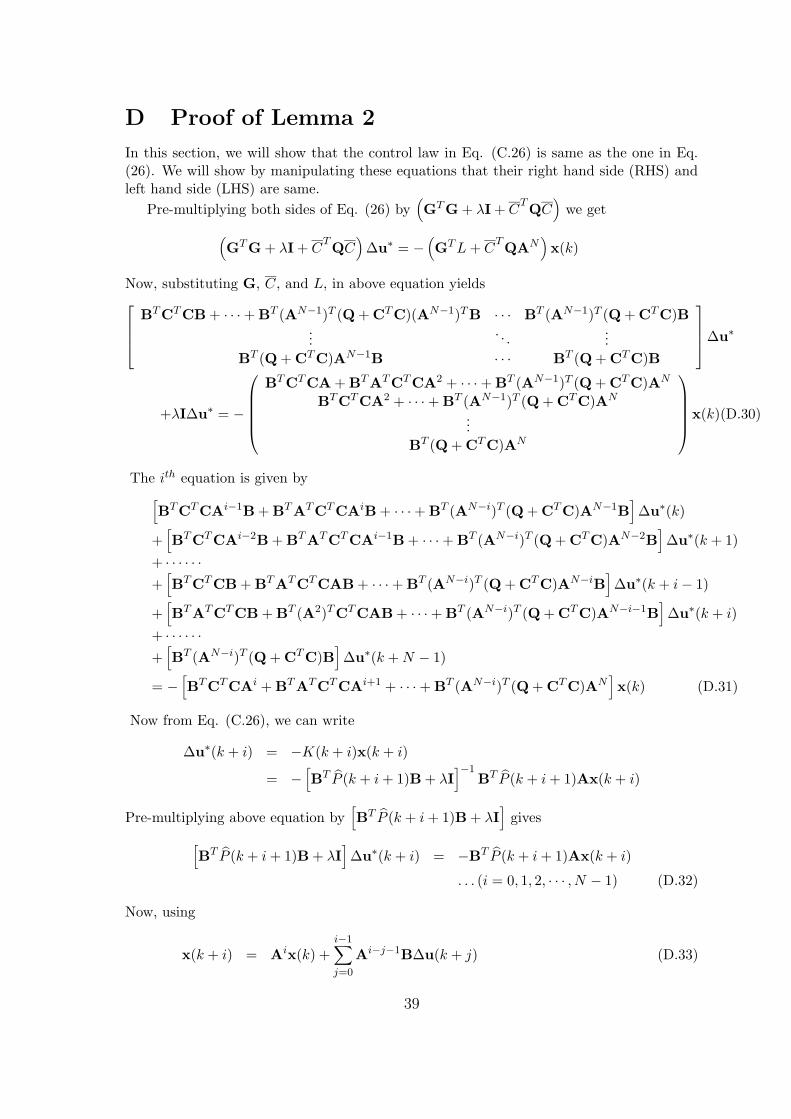
D Proof of Lemma 2
In this section, we will show that the control law in Eq. (C.26) is same as the one in Eq.(26). We will show by manipulating these equations that their right hand side (RHS) andleft hand side (LHS) are same.
Pre-multiplying both sides of Eq. (26) by(GTG + λI + C
TQC
)we get
(GTG + λI + C
TQC
)∆u∗ = −
(GT L + C
TQAN
)x(k)
Now, substituting G, C, and L, in above equation yields
Pre-multiplying above equation by[BT P (k + i + 1)B + λI
]gives
[BT P (k + i + 1)B + λI
]∆u∗(k + i) = −BT P (k + i + 1)Ax(k + i)
. . . (i = 0, 1, 2, · · · , N − 1) (D.32)
Now, using
x(k + i) = Aix(k) +i−1∑
j=0
Ai−j−1B∆u(k + j) (D.33)
39
= Aix(k) +[
Ai−1B Ai−2B · · · B]
∆u(k)∆u(k + 1)
...∆u(k + i − 1)
(D.34)
we can write Eq. (D.32) as
BT P (k + i + 1)[
AiB Ai−1B · · · Ai−1B B]
∆u∗(k)∆u∗(k + 1)
...∆u∗(k + i)
+λI∆u∗(k + i) = −BT P (k + i + 1)Ai+1x(k) (i = 0, 1, 2, · · · , N − 1)
Substituting for index i, we get
BT P (k + 1)B
BT P (k + 2)AB BT P (k + 2)B...
.... . .
BT P (k + N)AN−1B BT P (k + N)AN−2B · · · BT P (k + N)B
∆u∗(k)∆u∗(k + 1)
...∆u∗(k + N − 1)
︸ ︷︷ ︸∆u∗
+λI∆u∗ = −
BT P (k + 1)A
BT P (k + 2)A2
...
BT P (k + N)AN
x(k) (D.35)
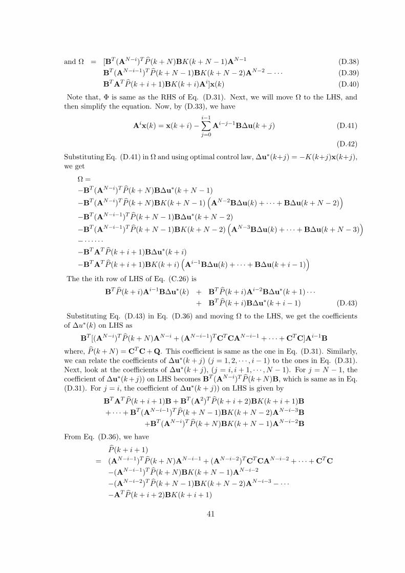
Note that Eqs. (D.30) and (D.35) have similar structure. Now, if we transform the RHSof Eq. (D.35) to match that of Eq. (D.30) and, as a result, if we get the LHS of bothequations to match we have proved the lemma.
So, first transform the RHS of Eq. (D.35) to match that of Eq. (D.30). Consider theith row in the RHS of Eq. (D.35). By Eq. (C.25), we have
P (k + i) = AT P (k + i + 1)A + CTC − AT P (k + i + 1)BK(k + i)
= AT [AT P (k + i + 2)A + CTC − AT P (k + i + 2)BK(k + i + 1)]A + CTC
where, P (k + N) = CTC + Q. This coefficient is same as the one in Eq. (D.31). Similarly,we can relate the coefficients of ∆u∗(k + j) (j = 1, 2, · · · , i − 1) to the ones in Eq. (D.31).Next, look at the coefficients of ∆u∗(k + j), (j = i, i + 1, · · · , N − 1). For j = N − 1, thecoefficient of ∆u∗(k + j)) on LHS becomes BT (AN−i)T P (k +N)B, which is same as in Eq.(D.31). For j = i, the coefficient of ∆u∗(k + j)) on LHS is given by
BTAT P (k + i + 1)B + BT (A2)T P (k + i + 2)BK(k + i + 1)B
+ · · · + BT (AN−i−1)T P (k + N − 1)BK(k + N − 2)AN−i−3B
−(AN−i−2)T P (k + N − 1)BK(k + N − 2)AN−i−3 − · · ·
−AT P (k + i + 2)BK(k + i + 1)
41
Substituting P (k + i + 1), we get the coefficient of ∆u∗(k + i) as follows
BT (AN−i)T P (k + N)AN−i−1B + BT (AN−i−1)TCTCAN−i−2B
+ · · · + BTATCTCB
which is same as the one in Eq. (D.31).Thus, we have shown that the optimal control law given by Eq. (26) is same as the one
given by Eq. (C.26)
Numerical Example:
Consider an LTI system,
x(k + 1) = Ax(k) + B∆u(k)
y(k) = Cx(k)
where
A =
[1 23 1
], B =
[01
], C =
[1 2
]
and the cost function of Eq. (22). Let the GPC control parameters be λ = 1, N1 = 1,N2 = Nu = 3, and
Q = [1] .
Now the GPC control law computed by Eq. (26) yields
Kgpc = (GTG + λI + CTQC)−1(CQA3 + GT L)
=
3.6368 2.46841.8240 3.10170.1072 −0.3723
Similarly, the LQ control law computation for the same cost function using Eq. (D.35)yields
Klqr =
BT P (1)B + λ
BT P (2)AB BT P (2)B + λ
BT P (3)A2B BT P (3)AB BT P (3)B + λ
−1
BT P (1)A
BT P (2)A2
BT P (3)A3
=
3.6368 2.46841.8240 3.10170.1072 −0.3723
which is same as Kgpc. This shows that both control laws are the same at time instantt = k. When the cost horizons for GPC and LQ strategies are identical.