Page 1
University of New MexicoUNM Digital Repository
Electrical and Computer Engineering ETDs Engineering ETDs
9-12-2014
GPGPU-Enabled Physics Based Deformed ModelSimulationAlejandro Enedino Hernandez Samaniego
Follow this and additional works at: https://digitalrepository.unm.edu/ece_etds
This Thesis is brought to you for free and open access by the Engineering ETDs at UNM Digital Repository. It has been accepted for inclusion inElectrical and Computer Engineering ETDs by an authorized administrator of UNM Digital Repository. For more information, please [email protected] .
Recommended CitationHernandez Samaniego, Alejandro Enedino. "GPGPU-Enabled Physics Based Deformed Model Simulation." (2014).https://digitalrepository.unm.edu/ece_etds/116
Page 2
%PINERHVS)RIHMRS,IVRERHI^7EQERMIKS
)PIGXVMGERH'SQTYXIV)RKMRIIVMRK
=MR=ERK
;IM;IRRMI7LY
1EVMSW74EXXMGLMW
M
Page 3
GPGPU-Enabled Physics BasedDeformed Model Simulation
by
Alejandro Enedino Hernandez Samaniego
B.S., Chihuahua Institute of Technology, 2011
THESIS
Submitted in Partial Fulfillment of the
Requirements for the Degree of
Master of Science
Computer Engineering
The University of New Mexico
Albuquerque, New Mexico
July, 2014
Page 4
c©2014, Alejandro Enedino Hernandez Samaniego
iii
Page 5
Dedication
To both my parents, Enedino and Patricia for always being supportive of my dreams.
“UNIX is basically a simple operating system, but you have to be a genius to
understand the simplicity” – Dennis M. Ritchie
iv
Page 6
Acknowledgments
I would like to thank my advisors, professor Yin Yang and professor Wei WennieShu, for their support, and professor Thomas Caudell, for being an excellent teacher,inspiring me to one day become one myself.
I also would like to thank:
CONACYT (Consejo Nacional de Ciencia y Tecnologıa), and the government ofthe United States of Mexico for giving me the opportunity of continuing my educa-tion.
Professors from my alma mater: Instituto Tecnologico de Chihuahua, who not onlysupported me but also encouraged me to keep going and ultimately helped me alongthe way to get my scholarship.
v
Page 7
GPGPU-Enabled Physics BasedDeformed Model Simulation
by
Alejandro Enedino Hernandez Samaniego
B.S., Chihuahua Institute of Technology, 2011
M.S., Computer Engineering, University of New Mexico, 2014
Abstract
Computer simulation techniques are widely adopted nowadays in many areas like
manufacturing, engineering, graphics, animation, virtual reality and so on. However,
the standard finite element based simulation is notorious for its expensive compu-
tation. To address this challenge, I present a GPU-based parallel implementation
for simulating large elastic deformation. Classic modal analysis provides a set of
orthonormal bases vectors, which span a spectral space encoding the dynamics of
the elastic body. As each basis vector is orthogonal to each other, the computa-
tion is completely decoupled and can be well-fit into the modern GPGPU platform.
We further explore the latest feature of NVIDIA CUDA so that the result of GPU
computation can be directly used for upcoming rendering/visualization and a signif-
icant amount of overheads for transmitting data from client GPU and host CPU via
the PCI-Express bus are avoided. Real-time simulation is made possible with this
technique for many cases that otherwise is not possible.
vi
Page 8
Contents
List of Figures xi
List of Tables xiii
Glossary xiv
1 Introduction 1
1.1 Overview . . . . . . . . . . . . . . . . . . . . . . . . . . . . . . . . . . 1
1.2 Computer Simulation . . . . . . . . . . . . . . . . . . . . . . . . . . . 2
1.2.1 History . . . . . . . . . . . . . . . . . . . . . . . . . . . . . . . 2
1.2.2 OpenGL . . . . . . . . . . . . . . . . . . . . . . . . . . . . . . 5
1.3 Parallel Computing . . . . . . . . . . . . . . . . . . . . . . . . . . . . 6
1.3.1 History . . . . . . . . . . . . . . . . . . . . . . . . . . . . . . . 6
1.3.2 Classification . . . . . . . . . . . . . . . . . . . . . . . . . . . 8
1.3.2.1 Levels of Parallelism . . . . . . . . . . . . . . . . . . 8
vii
Page 9
Contents
1.3.2.2 Parallel Architectures . . . . . . . . . . . . . . . . . 10
1.3.3 GPU Computing Languages . . . . . . . . . . . . . . . . . . . 12
1.3.3.1 Brook . . . . . . . . . . . . . . . . . . . . . . . . . . 12
1.3.3.2 NVIDIA CUDA . . . . . . . . . . . . . . . . . . . . . 14
1.3.3.2.1 CUDA Hierarchy: SIMT Architecture
. . . . . . . . . . . . . . . . . . . . . . . . 15
1.3.3.3 OpenCL . . . . . . . . . . . . . . . . . . . . . . . . . 20
1.3.3.3.1 OpenCL Hierarchy :
. . . . . . . . . . . . . . . . . . . . . . . . 21
1.4 Conclusions . . . . . . . . . . . . . . . . . . . . . . . . . . . . . . . . 22
2 Rendering on OpenGL 24
2.1 OpenGL Primitives . . . . . . . . . . . . . . . . . . . . . . . . . . . . 24
2.2 OpenGL Rendering Pipeline . . . . . . . . . . . . . . . . . . . . . . . 26
2.2.1 Fixed Function Pipeline . . . . . . . . . . . . . . . . . . . . . 27
2.2.2 Programmable Function Pipeline . . . . . . . . . . . . . . . . 27
2.2.2.1 GLSL . . . . . . . . . . . . . . . . . . . . . . . . . . 29
2.3 Buffer Objects . . . . . . . . . . . . . . . . . . . . . . . . . . . . . . . 33
2.4 External Libraries . . . . . . . . . . . . . . . . . . . . . . . . . . . . . 37
2.4.1 GLUT . . . . . . . . . . . . . . . . . . . . . . . . . . . . . . . 37
2.4.2 GLEW . . . . . . . . . . . . . . . . . . . . . . . . . . . . . . . 38
viii
Page 10
Contents
2.4.3 GLM . . . . . . . . . . . . . . . . . . . . . . . . . . . . . . . . 39
3 Parallelization 40
3.1 Modal Warping . . . . . . . . . . . . . . . . . . . . . . . . . . . . . . 40
3.1.1 Rotational Part in a Small Deformation . . . . . . . . . . . . 41
3.1.1.1 Kinematics of Infinitesimal Deformation . . . . . . . 41
3.1.1.2 Extended Modal Analysis . . . . . . . . . . . . . . . 43
3.1.1.3 Modal Rotation . . . . . . . . . . . . . . . . . . . . . 44
3.1.2 Implementation . . . . . . . . . . . . . . . . . . . . . . . . . . 46
3.2 Analyze Stage . . . . . . . . . . . . . . . . . . . . . . . . . . . . . . . 48
3.2.1 GNU Profiler . . . . . . . . . . . . . . . . . . . . . . . . . . . 48
3.2.2 Amdahl’s Law . . . . . . . . . . . . . . . . . . . . . . . . . . . 50
3.2.3 Computer and device specs . . . . . . . . . . . . . . . . . . . 51
3.3 Parallelize Stage . . . . . . . . . . . . . . . . . . . . . . . . . . . . . . 53
3.3.1 Kernel Development . . . . . . . . . . . . . . . . . . . . . . . 54
3.4 Experimentation Results - Deploy Stage . . . . . . . . . . . . . . . . 69
3.5 Potential Improvements - Optimize Stage . . . . . . . . . . . . . . . . 72
3.5.1 OpenGL CUDA Interoperability . . . . . . . . . . . . . . . . . 75
3.6 Results . . . . . . . . . . . . . . . . . . . . . . . . . . . . . . . . . . . 77
4 Conclusion and Future Work 83
ix
Page 11
Contents
4.1 Limitations and Future Work . . . . . . . . . . . . . . . . . . . . . . 83
4.1.1 APU’s . . . . . . . . . . . . . . . . . . . . . . . . . . . . . . . 83
4.2 Conclusion . . . . . . . . . . . . . . . . . . . . . . . . . . . . . . . . . 91
A Appendix A - C++ Code 92
References 93
x
Page 12
List of Figures
1.1 Processor Performance Over Time[8] . . . . . . . . . . . . . . . . . . 7
1.2 GPU Computing Language Timeline [13] . . . . . . . . . . . . . . . 13
1.3 BrookGPU System Outline[14] . . . . . . . . . . . . . . . . . . . . . 14
1.4 Brook’s performance on 1st generation of programmable GPUs[14] . 15
1.5 CUDA Hierarchy [17] . . . . . . . . . . . . . . . . . . . . . . . . . . 17
1.6 CUDA Scalability [17] . . . . . . . . . . . . . . . . . . . . . . . . . . 17
1.7 Fermi Streaming Processor (CUDA Core) [18] . . . . . . . . . . . . . 18
1.8 Tesla Streaming Multiprocessor [12] . . . . . . . . . . . . . . . . . . 18
1.9 Fermi Streaming Multiprocessor [18] . . . . . . . . . . . . . . . . . . 19
1.10 Kepler Streaming Multiprocessor (SMX) [19] . . . . . . . . . . . . . 19
1.11 OpenCL Hierarchy [13] . . . . . . . . . . . . . . . . . . . . . . . . . 21
1.12 OpenCL Hierarchy [20] . . . . . . . . . . . . . . . . . . . . . . . . . 22
2.1 OpenGL 1.0 Fixed Pipeline [22] . . . . . . . . . . . . . . . . . . . . 27
2.2 OpenGL 4.3 Rendering Pipeline[7] . . . . . . . . . . . . . . . . . . . 28
xi
Page 13
List of Figures
2.3 Shader compilation process[7] . . . . . . . . . . . . . . . . . . . . . . 31
3.1 CUDA’s Default Stream Behavior . . . . . . . . . . . . . . . . . . . 68
3.2 CUDA’s Streams Behavior . . . . . . . . . . . . . . . . . . . . . . . 68
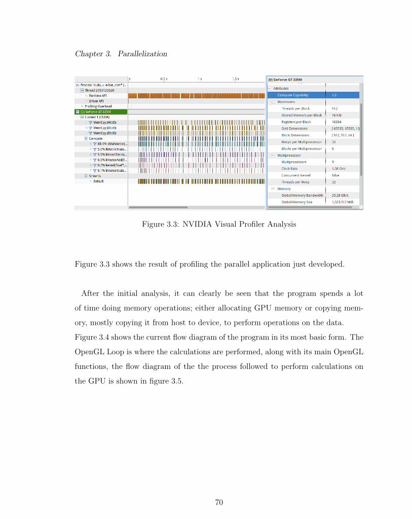
3.3 NVIDIA Visual Profiler Analysis . . . . . . . . . . . . . . . . . . . . 70
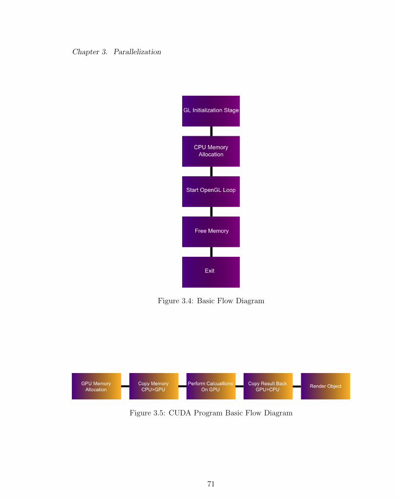
3.4 Basic Flow Diagram . . . . . . . . . . . . . . . . . . . . . . . . . . . 71
3.5 CUDA Program Basic Flow Diagram . . . . . . . . . . . . . . . . . 71
3.6 Basic Flow Diagram After Optimizations . . . . . . . . . . . . . . . 74
3.7 Performance by # Eigenvalues on Different Objects . . . . . . . . . 80
3.8 Performance by Object’s Size . . . . . . . . . . . . . . . . . . . . . . 80
3.9 Bar Analysis . . . . . . . . . . . . . . . . . . . . . . . . . . . . . . . 82
3.10 Armadillo Analysis . . . . . . . . . . . . . . . . . . . . . . . . . . . 82
4.1 Llano APU block diagram [31] . . . . . . . . . . . . . . . . . . . . . 85
4.2 Knapsack Algorithm on APU [32] . . . . . . . . . . . . . . . . . . . 86
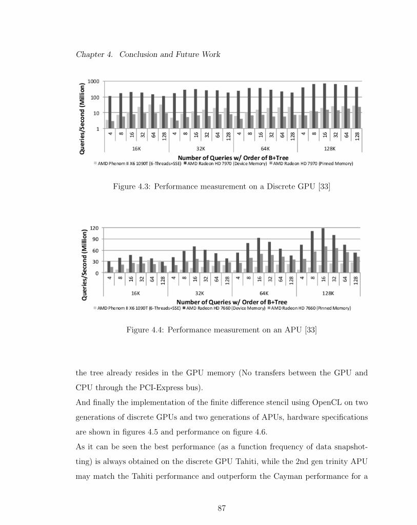
4.3 Performance measurement on a Discrete GPU [33] . . . . . . . . . . 87
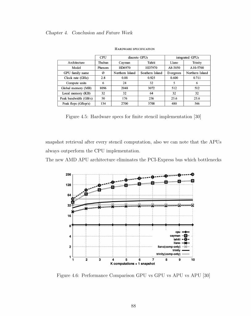
4.4 Performance measurement on an APU [33] . . . . . . . . . . . . . . 87
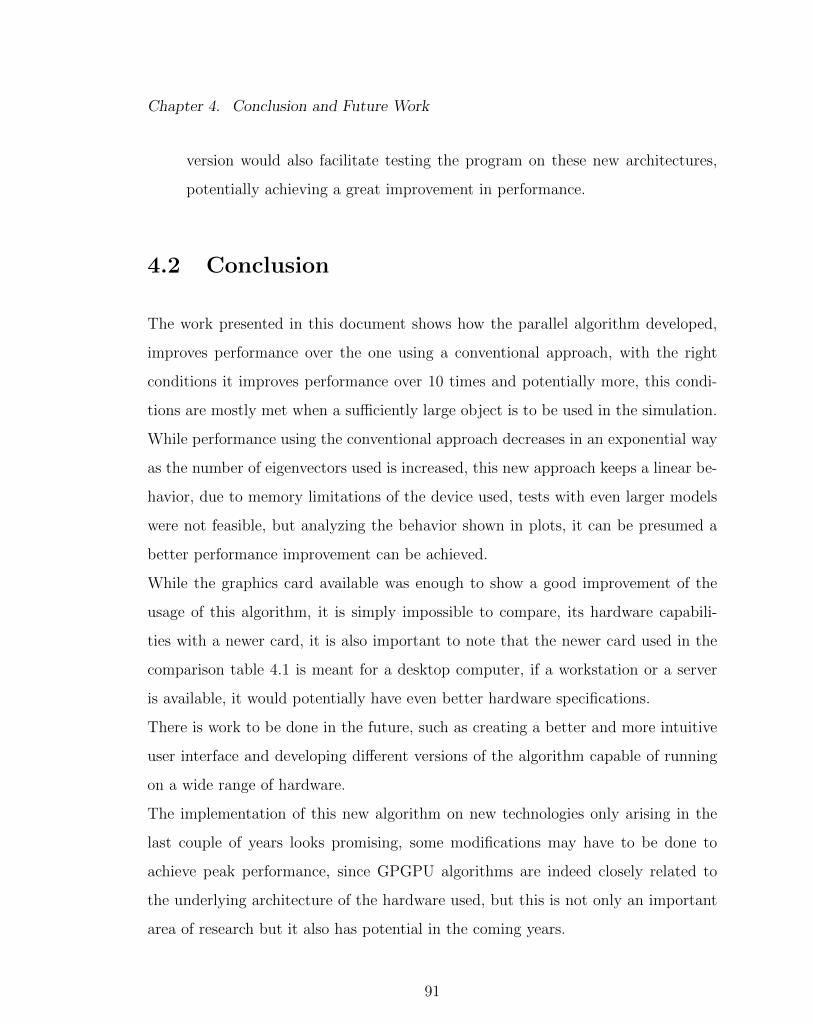
4.5 Hardware specs for finite stencil implementation [30] . . . . . . . . . 88
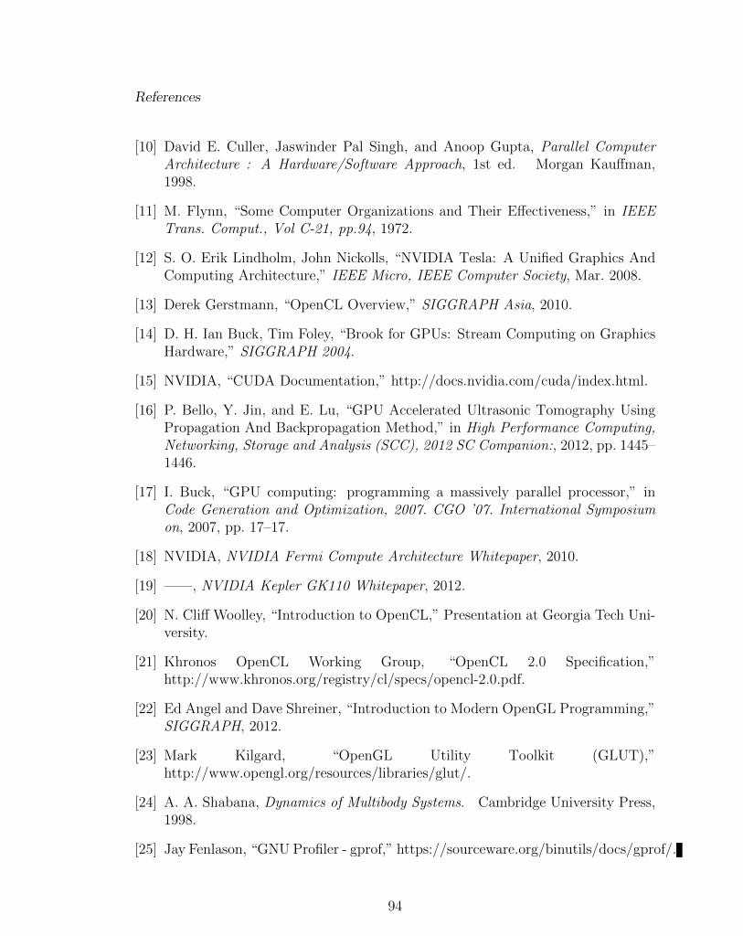
4.6 Performance Comparison GPU vs GPU vs APU vs APU [30] . . . . 88
xii
Page 14
List of Tables
2.1 Buffer Usage Tokens . . . . . . . . . . . . . . . . . . . . . . . . . . . 35
3.1 Initial Experimentation Results . . . . . . . . . . . . . . . . . . . . . 69
3.2 Objects Tested . . . . . . . . . . . . . . . . . . . . . . . . . . . . . . 78
3.3 Bar Performance Results . . . . . . . . . . . . . . . . . . . . . . . . 78
3.4 Sphere Performance Results . . . . . . . . . . . . . . . . . . . . . . 79
3.5 Cube Performance Results . . . . . . . . . . . . . . . . . . . . . . . 79
3.6 Armadillo Performance Results . . . . . . . . . . . . . . . . . . . . . 79
4.1 GPU Comparison . . . . . . . . . . . . . . . . . . . . . . . . . . . . 84
xiii
Page 15
Glossary
ALU Arithmetic Logic Unit.
API Accelerated Programming Interface.
APU Accelerated Processing Unit.
BLP Bit Level Parallelism.
CISC Complex Instruction Set Computer.
CPU Compute Processing Unit.
DLP Data Level Parallelism.
ENIAC Electronic Numerical Integrator and Computer.
FEM Finite Element Methods.
GPU Graphics Processing Unit.
GPGPU General Purpose Computing on Graphics Processing Units
GUI Graphical User Interface.
ILP Instruction Level Parallelism.
MIMD Multiple Instruction Multiple Data.
xiv
Page 16
Glossary
MISD Multiple Instruction Single Data.
RISC Reduced Instruction Set Computer.
SIMD Single Instruction Multiple Data.
SIMT Single Instruction Multiple Thread.
SISD Single Instruction Single Data.
SP Streaming Multiprocessor.
SP Streaming Processor.
STL Standard Template Library.
TLP Thread/Task Level Parallelism.
V AO Vertex Array Object.
V BO Vertex Buffer Object.
xv
Page 17
Chapter 1
Introduction
1.1 Overview
The work described in this document aims to implement a deformed model simu-
lation algorithm in parallel on the GPU (Graphics Processing Unit) using modal
warping, based on physics techniques to approximate the behavior of an object when
its subject totally or partially to a force applied. Using the architectural advantages
of GPUs, this GPGPU (General Purpose Computing on the GPU) algorithm can
be implemented efficiently even with a small device, obtaining a considerable speed
improvement over conventional algorithms and also providing accurate results.
In the following sections an explanation of why certain tools such as computer lan-
guages were chosen and how they were used to implement the algorithm can be
found.
1
Page 18
Chapter 1. Introduction
1.2 Computer Simulation
1.2.1 History
Computer simulation has become one of the most important areas of research in
the last couple of decades, its history dates back to the World War II era, when 2
mathematicians: John Von Neumann and Stanislaw Ulam, faced the complicated
problem of neutrons behavior.
Stan made the following remarks about his ideas in the 1980’s:
” The first thoughts and attempts I made to practice the Monte Carlo method, were
suggested by a question which occurred to me in 1946 as I was convalescing from an
illness and playing solitaires. The question was: what are the chances that a Canfield
solitaire laid out with 52 cards will come out successfully?, After spending a lot of
time trying to estimate them by pure combinational calculations, I wondered whether
a more practical method than ”abstract thinking” might not be to lay it out say one
hundred times and simply observe and count the number of successful plays. This
was already possible to envisage with the beginning of the new era of fast computers,
and I immediately thought of problems of neutron diffusion and other questions of
mathematical physics, more generally how to change processes described by certain
differential equations into an equivalent form interpretable as a succession of random
operations. Later... in 1946 I described the idea to John Von Neumann and we began
to plan the actual calculations”.[1]
Von Neumann was intrigued, doing statistical sampling using newly developed elec-
tronic computing techniques seemed a great idea, in March of 1947 Von Neumann
wrote a letter to Robert Richtmyer, who was the Theoretical Division Leader at
2
Page 19
Chapter 1. Introduction
Los Alamos National Laboratory, where he concluded: ”the statistical approach is
very well suited to a digital treatment”, he outlined in some detail how this method
could be used to solve neutron diffusion and multiplication problems in fission de-
vices,further details about this method lay beyond the scope of this document.
Finally at the end of the letter, Von Neumann attached a tentative ”computing
sheet”, that he felt would serve as a basis for setting up this calculation on the
ENIAC, the ENIAC was the first general purpose computer built in secret at the
University of Philadelphia’s Moore’s School of Electrical Engineering [2].
The outline was the first formulation of a Monte Carlo computation for an electronic
machine.
From that moment on, hardware always predominated the simulation field, it wasn’t
until the 1950’s when programming languages began to emerge and computer simu-
lation started to be developed in several different areas. Computer simulations main
applications vary in different areas nowadays, such as:
• Medical
• Science
• Physics
• Engineering
• Military
One of the specific areas of research in computer simulation is deformable model
simulation, which is also applied in all the areas stated before.
This area has specifically been subject of research in the past three decades, the rea-
son being that, until the 1980’s computer based modelling techniques only allowed
modelling of rigid bodies. In 1984 a series of geometric operators for deforming a
3
Page 20
Chapter 1. Introduction
solid object by transforming the coordinate space were introduced [3]. These were
the starting point for the development of better and improved techniques for de-
formed object modelling.
Computer based deformed modelling techniques are classified in non-physical, phys-
ical and approximate physical techniques:
• Non-Physical Techniques: Purely geometric techniques used to deform virtual
objects, accuracy is sacrificed for more computational efficiency.
– Splines and Patches.
– Free Form Deformation.
• Physical Techniques: Based on principles of continuum mechanics applied to a
geometric structure of a model, these techniques sacrifice computational com-
plexity but provide a more accurate, and realistic result.
– Discrete Models: Mass Spring Damper Methods.
– Continuum Models: Finite Element Methods (FEM).
• Approximate Physical Techniques: These techniques are not derived directly
from continuum mechanics equations, although they are physically motivated.
– Active Contour Models
4
Page 21
Chapter 1. Introduction
While non-physical techniques are the most efficient and more simply imple-
mented computationally speaking, accuracy is also greatly sacrificed, the most widely
used techniques are physical based techniques [4], where FEM are state of the art
in physically based modelling becoming more used in the last few years as computa-
tional power increases.
Physics based techniques are more complex computationally speaking due to the
fact that they handle nonlinearities, this has the main advantage of providing a
more accurate and realistic result, but it becomes complex, for this specific case,
handling nonlinearities would not easily allow for a parallel algorithm to be created,
but omitting the nonlinear term would create unrealistic results, increasing the vol-
ume of the model inaccurately.
The modal warping technique used in this work omits the nonlinear term initially
when precomputing, although once the simulation is being run, the rotation infor-
mation is kept, even when the object is deformed, the precomputed modal basis is
warped according to the rotational information obtained [5], giving a realistic result
but also providing the opportunity of approaching the problem in a parallelizable
way.
A more profound classification survey and explanation of these techniques and their
advantages and disadvantages can be found on [6] and [4].
1.2.2 OpenGL
OpenGL is merely an API; a software library for accessing features in graphics hard-
ware, as of today it contains more than 500 different commands, used to specify
objects, images and operations needed to produce interactive 3-dimensional com-
5
Page 22
Chapter 1. Introduction
puter graphics applications[7].
OpenGL is designed to be implemented on many different types of graphics hard-
ware, or it could even be implemented entirely in software, it is also independent of
the operating system the computer is running on, due to this type of implementa-
tion, some limitations may be considered, it does not provide functions to process
user input or creating windows, which means it needs to be used along with some
other library that performs this functions and complement it, OpenGL also has the
limitation if it may be called that, that lacks a functionality for describing models or
3D objects in any way, neither to read files of any sort. Instead the programmer must
read these files or construct the 3D objects from a small set of geometric primitives
(points, lines, triangles, etc.) these primitives will be explained in further detail on
section 2.1 of this document.
1.3 Parallel Computing
1.3.1 History
Computer technology made incredible progress in over 60 years since the first gen-
eral purpose computer was created, if we analyze the progress over time, we see that
during the first 25 years, progress was made in both creating new architectures and
developing new technologies, delivering a raise of approximately 25% per year on
performance.
By 1970 when the microprocessor emerged, it led to a higher rate of performance
improvement, around 35% per year.
In the early 1980’s a set of changes made possible the development of RISC (Re-
duced Instruction Set Computer), which used new performance techniques such as
instruction level parallelism and the use of caches, this started what some people
6
Page 23
Chapter 1. Introduction
Figure 1.1: Processor Performance Over Time[8]
call the hardware renaissance of computers, where a 52% of improvement per year
was achieved. As figure 1.1 shows, the renaissance ended on the year of 2003, this
happened because as time passed transistors got smaller, faster and used less power,
so processor makers not only added more and more transistors on the same chip, but
they also increased the clock frequency of processors.
The question is: Why did they stop?. The simplest answer to that power, both
power and heat are the main issue when developing a microprocessor, due to the fact
that a billion of transistors generate a lot of heat , and when running at that speed
it is impossible to keep the chip from melting. The CPU’s or main processors may
have been hurt by this parameter, but GPUs have not, or at least not in the same
way, due to the fact that GPUs are different in architecture, they have a lot more of
compute units or ALU’s (Arithmetic Logic Units), but each of those is a lot simpler
7
Page 24
Chapter 1. Introduction
too, they have small caches, memory accesses are extremely coherent, and memory
modules are usually a lot faster than the ones used for CPU’s (also known as system
memory), this means that when we have a problem which can be organized in a way
that there are a wide amount simple computations to do, instead of small amount of
complex ones, GPUs are a good option to solve this type of problem [9].
1.3.2 Classification
There are several types of different parallelization techniques, they are mainly clas-
sified according to how the calculations are organized to be computed in parallel.
1.3.2.1 Levels of Parallelism
Parallelism can be characterized in levels or forms of where the parallelism is applied
to, which could be exploited differently depending on the parallel architecture. Lev-
els of parallelism may be classified as follows:
• Bit Level Parallelism (BLP): BLP is a form of parallelism achieved by increas-
ing the processor word size, doing so reduces the number of instructions the
processor has to execute in order to perform an operation on variables whose
sizes are greater than the length of the processor word size, an addition between
two 32-bit integers using a 16-bit processor, requires the processor to first add
the 16 lower order bits from each of the integers and then add the 16 higher
order bits, requiring two instructions to complete a single operation [10].
• Instruction Level Parallelism (ILP): ILP is a form of parallelism achieved by
applying different techniques to the instructions sent to the processor, tech-
8
Page 25
Chapter 1. Introduction
niques such as pipelining, which overlaps the execution of instructions and
improves performance, or loop unrolling, performing several loop operations
in just one cycle instead of one operation per cycle, limitations for this type
of parallelism include data dependencies and control hazards, when exploiting
this type of parallelism one must be sure that the data is independent from one
cycle to another, otherwise those 2 or more instructions cannot be executed
simultaneously or be completely overlapped, and also that the instructions are
not control dependent, meaning that the order in which the instructions are
executed does not matter, since it cannot be known for sure which operation
will be executed first when executed in parallel.
There are 2 main approaches for exploiting ILP, an approach that relies on
hardware to help discover and exploit the parallelism dynamically, and an
approach relying on software technology to find parallelism statically at compile
time [8].
• Data Level Parallelism (DLP): DLP is a form of parallelism where parallelism is
focused on the data itself, in a multiprocessor system when executing a single
set of instructions (SIMD) 1.3.2.2, data parallelism is achieved when each
processor performs the same computations on different pieces of distributed
data.
• Thread/Task Level Parallelism (TLP): TLP is a form of parallelism, focused
on distributing execution processes or threads across different computer nodes,
or processors, this is achieved when a thread or process is executed on each
different processor, where this threads may execute the same or different code
and on the same or different data, this form of parallelization requires inter-
communication amongst threads, in general TLP is more flexible than DLP
and thus more generally applicable[8].
9
Page 26
Chapter 1. Introduction
1.3.2.2 Parallel Architectures
The most popular characterization of different types of parallel architectures was
defined by Flynn in 1966 [11] and is specified as follows:
• SISD: Simple Instruction Simple Data - Conventional single processors com-
puters are classified as SISD systems, each arithmetic instruction initiates an
operation on a data item taken from a single stream of data elements.
• SIMD: Simple Instruction Multiple Data - The same instruction is executed by
multiple processors using different data streams, these type of systems exploit
DLP (Data Level Parallelism), by applying the same operations to multiple
items of data in parallel. In these type of systems each processor has its own
data memory, but there is only one instruction memory and control processor,
whose function is to fetch and dispatch instructions. There are three main
variants of SIMD: Vector Architectures, Multimedia SIMD Set extensions and
GPUs.
Given the fact that in this work I use a variant of SIMD’s I will explain a little
further each of these:
– Vector Architectures:
Vector architectures grab sets of data elements scattered in memory, place
them into large, sequential register files, operate on the data in those reg-
ister files and then disperse the results back into memory.
A single instruction operates on vectors of data, which in turn, results
in dozens of register-register operations on independent data elements.
These register files act as compiler-controlled buffers, both hide mem-
ory latency and leverage memory bandwidth, vector loads/stores are also
10
Page 27
Chapter 1. Introduction
deeply pipelined, so the program pays the long memory latency only once
per load/store instruction instead of doing it on every element.
– Instruction Set Extensions For Multimedia:
These extensions as the name implies are often used for multimedia pur-
poses or applications, since many of these applications operate on nar-
rower data types, than what conventional processors are optimized for,
they can be used for audio, graphics, etc. An instruction specifies the
same operation on vectors of data, but unlike vector architectures, which
have register files, these instructions tend to specify fewer operands and
use much smaller registers.
– Graphic Processing Units:
This variation of the SIMD taxonomy, offers high potential performance,
GPUs share some features with vector architectures, but they also have
their own distinguishing characteristics, these systems have a conventional
system processor and a system memory in addition to their own process-
ing units and graphics memory, that is why these systems are often called
heterogeneous [8]. Although GPUs do fall inside this category, this ex-
plains their functionality mainly for what they were initially developed
for: computer graphics; when these are utilized to perform GPGPU or in
other words, for applications traditionally handled by the CPU, they fall
into a new category (not part of Flynn’s taxonomy) SIMT (Simple In-
struction Multiple Thread) [12] which will be explained in further detail
later in this document 1.3.3.2.1 .
• MISD: Multiple Instruction Simple Data - Multiple instruction streams and a
single data stream, no commercial multiprocessor of this type has been built
11
Page 28
Chapter 1. Introduction
to this date.
• MIMD: Multiple Instruction Multiple Data - Multiple instruction streams and
also multiple data streams, where each processor fetches its own instructions
and operates on its own data, these type of systems exploit TLP (Thread Level
Parallelism) 1.3.2.1.
Although Flynn’s taxonomy characterizes very well the majority of commercial par-
allel architectures, it is a coarse model, and some multiprocessors are hybrids of these
categories.
1.3.3 GPU Computing Languages
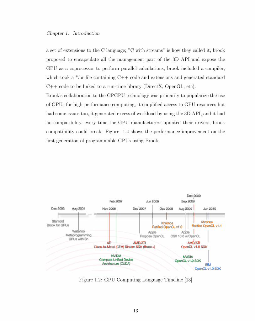
GPU languages first appeared in 2003, it is shown how they have evolved over the
years in figure 1.2.
1.3.3.1 Brook
Back in the year 2003: Brook, or BrookGPU appeared [14], developed at Stanford
University, researchers realized GPUs could also be used to perform general com-
puting calculations, due to their underlying architecture, but at the time, the only
way to access GPUs resources was to use one of the graphics API’s (Application
Programming Interfaces): OpenGL or Direct3D, so researchers had to use them if
they wanted to perform calculations on the GPU, the problem was that one had to
become an expert in graphics programming to do this, which seriously complicated
things, since graphics programmers think in terms of shaders and textures, while
parallel programmers think in terms of kernels or streams. Brook was presented as
12
Page 29
Chapter 1. Introduction
a set of extensions to the C language; ”C with streams” is how they called it, brook
proposed to encapsulate all the management part of the 3D API and expose the
GPU as a coprocessor to perform parallel calculations, brook included a compiler,
which took a *.br file containing C++ code and extensions and generated standard
C++ code to be linked to a run-time library (DirectX, OpenGL, etc).
Brook’s collaboration to the GPGPU technology was primarily to popularize the use
of GPUs for high performance computing, it simplified access to GPU resources but
had some issues too, it generated excess of workload by using the 3D API, and it had
no compatibility, every time the GPU manufacturers updated their drivers, brook
compatibility could break. Figure 1.4 shows the performance improvement on the
first generation of programmable GPUs using Brook.
Figure 1.2: GPU Computing Language Timeline [13]
13
Page 30
Chapter 1. Introduction
1.3.3.2 NVIDIA CUDA
Brook’s success was enough to attract the attention of both major GPU manufac-
turing companies: ATI and specially of NVIDIA, so Brook’s researchers got into
development teams at NVIDIA’s headquarters with the idea of offering hardware/-
software suited for this type of calculations. But, since NVIDIA architects and
developers knew all about their own design there was no need to rely on graphics
API’s anymore, and they were able to design a set of software layers to communicate
with the GPU: CUDA (Compute Unified Device Architecture) [15].
CUDA provides 2 API’s:
• CUDA Runtime API (High-Level)
• CUDA Driver API (Low-Level)
Figure 1.3: BrookGPU System Outline[14]
14
Page 31
Chapter 1. Introduction
Although, each call to a function of the high level API is broken down into more
basic instructions managed by the low level API.
The CUDA Runtime API can be considered as very low level too, since it requires
knowledge of the hardware that is being used, but it still offers functions that are
highly practical in terms of initialization and context management.
Both API’s are able to communicate with graphics libraries such as Direct3D and
OpenGL, this is useful since one can generate resources using CUDA and these can
be passed to the graphics API, the advantage here being that the resources remain
stored in GPUs RAM without having to transit through the bottleneck of the PCI-
Express bus.
1.3.3.2.1 CUDA Hierarchy: SIMT Architecture
CUDA extends the C programming language by allowing the programmer to define
C parallel functions called kernels, when called, these functions are executed N times
Figure 1.4: Brook’s performance on 1st generation of programmable GPUs[14]
15
Page 32
Chapter 1. Introduction
in parallel by N different CUDA threads as opposed to regular C functions. Note
that originally the kernels could only be ”launched” from using the CPU, although
has NVIDIA introduced the Kepler architecture featuring the ability to launch ker-
nels from the GPU without CPU involvement.
Each thread that executes the kernel has its own local memory, and its given a
unique thread ID, which is accessible within the kernel. This unique ID variable is a
3 component vector or 3 dimensional vector.
These threads are organized in warps, warps are groups of 32 threads, which is the
minimum size of the data processed in SIMD by a CUDA SM (Streaming Multipro-
cessor). Due to granularity issues in CUDA; instead of manipulating warps directly,
threads are organized into blocks that can contain from 64 to 1024 threads on current
GPUs, and they all share a memory called ”shared memory”.
CUDA capable devices use this new execution model or architecture called SIMT
to manage and execute thousands of threads efficiently, which were both first intro-
duced by NVIDIA in 2006 with the G80 (Tesla Family) of GPUs [12].
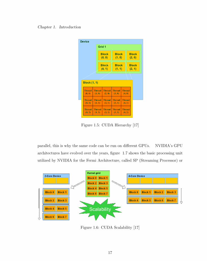
Finally these blocks are organized into a one-dimensional, two-dimensional or three-
dimensional grid, where the number of thread blocks in a grid is usually dictated
by the size of the data being processed or the number of processors in the system,
this is where a the global memory is used, it is the slowest of them all but it can be
accessed from any threads on the device [16]. The advantage of grouping them in this
sort of hierarchy is that the number of blocks processed simultaneously by the GPU
are closely linked to the architecture of the GPU (hardware resources), the number
of blocks in a grid make it possible to totally abstract that constraint and apply a
kernel to a large quantity of threads in a single call, without worrying about fixed re-
sources. The CUDA Runtime library takes care of that, making this model extremely
extensible, if the GPU has only a few resources it executes the blocks sequentially,
but if it has a large number of processing units instead, it can process them all in
16
Page 33
Chapter 1. Introduction
Figure 1.5: CUDA Hierarchy [17]
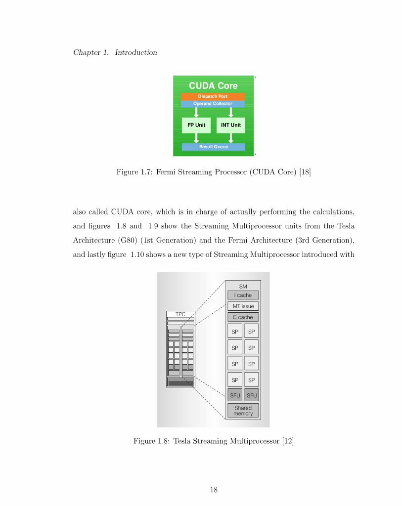
parallel, this is why the same code can be run on different GPUs. NVIDIA’s GPU
architectures have evolved over the years, figure 1.7 shows the basic processing unit
utilized by NVIDIA for the Fermi Architecture, called SP (Streaming Processor) or
Figure 1.6: CUDA Scalability [17]
17
Page 34
Chapter 1. Introduction
Figure 1.7: Fermi Streaming Processor (CUDA Core) [18]
also called CUDA core, which is in charge of actually performing the calculations,
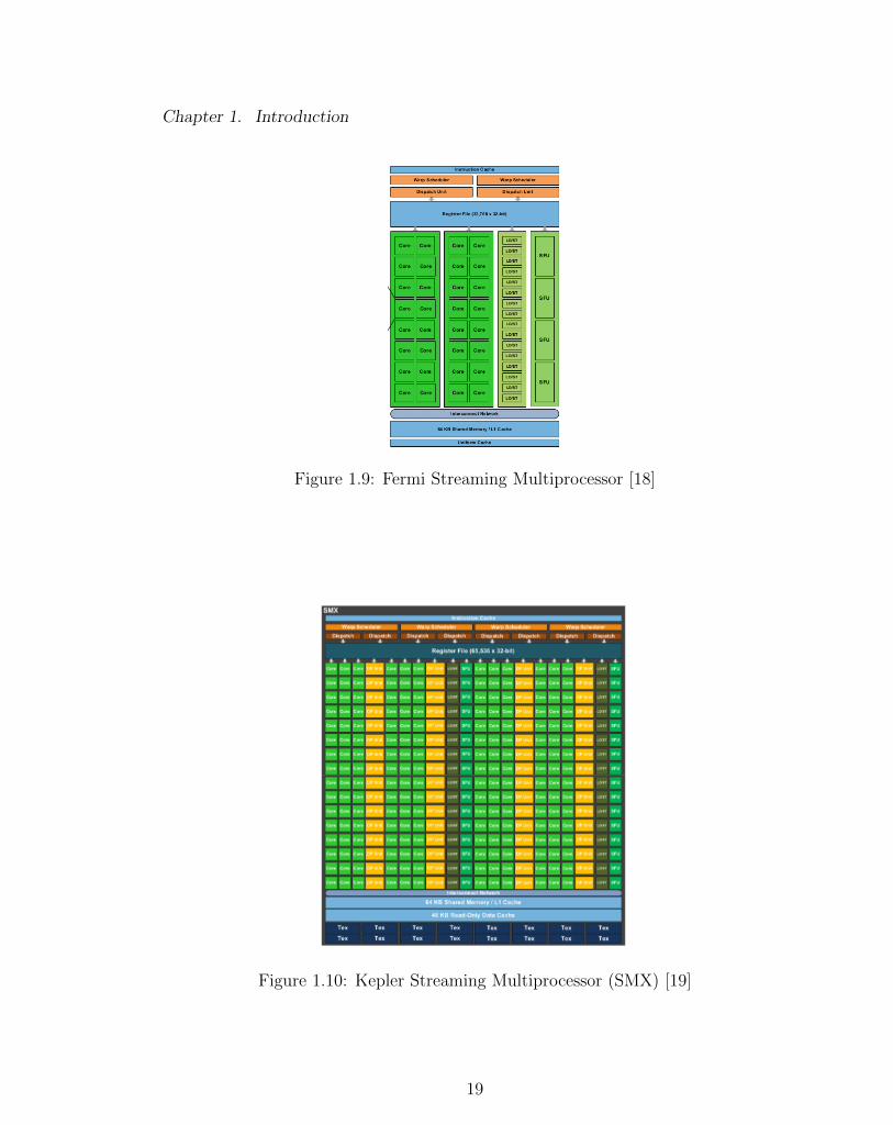
and figures 1.8 and 1.9 show the Streaming Multiprocessor units from the Tesla
Architecture (G80) (1st Generation) and the Fermi Architecture (3rd Generation),
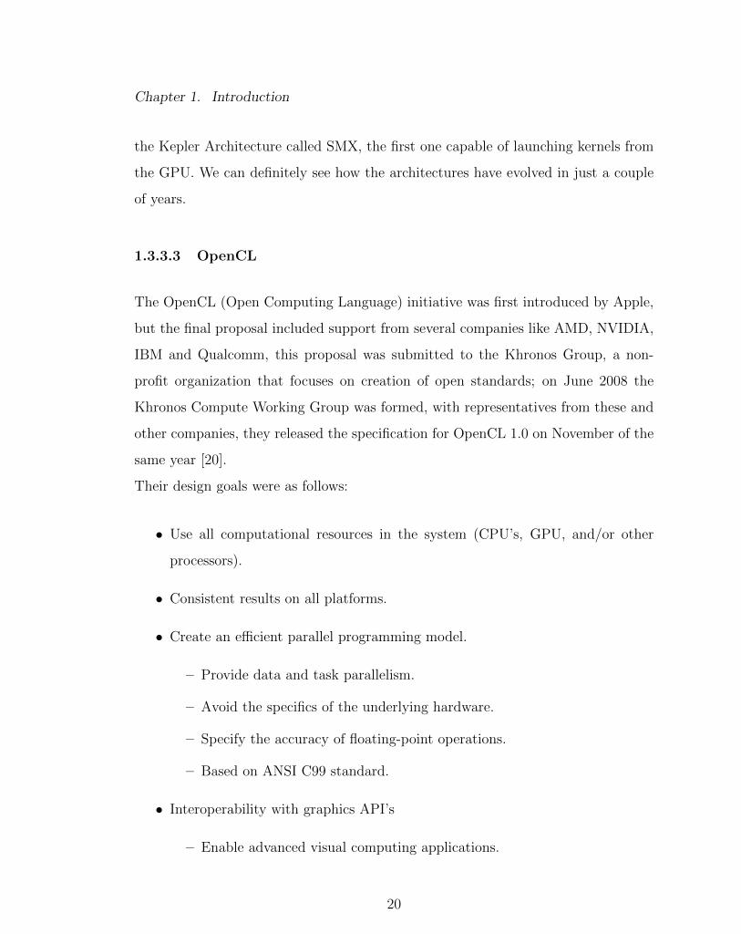
and lastly figure 1.10 shows a new type of Streaming Multiprocessor introduced with
Figure 1.8: Tesla Streaming Multiprocessor [12]
18
Page 35
Chapter 1. Introduction
Figure 1.9: Fermi Streaming Multiprocessor [18]
Figure 1.10: Kepler Streaming Multiprocessor (SMX) [19]
19
Page 36
Chapter 1. Introduction
the Kepler Architecture called SMX, the first one capable of launching kernels from
the GPU. We can definitely see how the architectures have evolved in just a couple
of years.
1.3.3.3 OpenCL
The OpenCL (Open Computing Language) initiative was first introduced by Apple,
but the final proposal included support from several companies like AMD, NVIDIA,
IBM and Qualcomm, this proposal was submitted to the Khronos Group, a non-
profit organization that focuses on creation of open standards; on June 2008 the
Khronos Compute Working Group was formed, with representatives from these and
other companies, they released the specification for OpenCL 1.0 on November of the
same year [20].
Their design goals were as follows:
• Use all computational resources in the system (CPU’s, GPU, and/or other
processors).
• Consistent results on all platforms.
• Create an efficient parallel programming model.
– Provide data and task parallelism.
– Avoid the specifics of the underlying hardware.
– Specify the accuracy of floating-point operations.
– Based on ANSI C99 standard.
• Interoperability with graphics API’s
– Enable advanced visual computing applications.
20
Page 37
Chapter 1. Introduction
Figure 1.11: OpenCL Hierarchy [13]
– Efficient resource sharing for graphics data.
– Support graphics oriented built-in methods.
Then OpenCL is defined as: ”The open standard for developing cross-platform, ven-
dor agnostic, parallel programs that run on current and future multi-core processors
within workstations, desktops, notebooks and mobile devices”. OpenCL 2.0 specifi-
cation was released on November 14th, 2013 , and it supports the following vendors:
NVIDIA, AMD, Apple, Samsung, Qualcomm, ARM, Intel, IBM and others [21].
1.3.3.3.1 OpenCL Hierarchy :
In OpenCL programs are divided in 2 parts: One that executes on the device
(GPU) and the other that executes on the host (CPU); code that is to be executed
on the device must be inside a kernel and is where all the parallelism must happen,
these kernels can only be called from the host. Much like NVIDIA’s CUDA, OpenCL
kernels are executed N times in parallel by N different work-items, which are the
smallest execution entity, each work-item has its own ID, accessible from the kernel
and distinguishes it from the other ones, making it possible to process different data,
every work-item also has its own memory, referred to as private memory. Work-
21
Page 38
Chapter 1. Introduction
Figure 1.12: OpenCL Hierarchy [20]
items are grouped into work-groups, where they can share a memory called local
memory, these work groups also have their unique ID. Finally the work groups are
organized into an N-Dimensional grid called ND-Range, where N=1,2 or 3, and a
global memory is shared between the whole grid.
1.4 Conclusions
The work explained in section 3.1 was initially thought to be developed using MAT-
LAB, it was, and it provided advantages over the previous related work, being able
to accurately simulate rotations on large objects, but MATLAB libraries still pro-
vided a slower and slower rendering and computations as the object became larger
and larger, performance started to become an issue, that motivated the work ex-
plained in this document, to be able to provide not only a better and more efficient
renderer engine; using OpenGL, but also to be able to perform the computations
22
Page 39
Chapter 1. Introduction
faster, doing this in a compiled language such as C or C++, if programmed cor-
rectly, would have provided better results than the ones obtained using MATLAB,
although a better option was to use parallel programming on the GPU (GPGPU),
since the modal warping method efficiently decouples the physics equations on which
the simulation is based, making calculations independent from each other, it requires
a vast amount of operations on matrices, which also may be computed on an element
by element basis on independent data, meaning that an operation to compute ele-
ment i is independent on the one used to compute element j, these type of operations
are a perfect example to use parallel programming and more specifically on the GPU.
The parallel version was programmed using C++ as its main language, OpenGL was
used to program the renderer for the 3 dimensional object simulation, and CUDA
as its parallel programming platform, it must be noted that as explained in section
1.3.3.3 OpenCL and CUDA programming models are very similar, meaning that in
the future would allow for an OpenCL version to be developed ”easily” based on the
already existing version programmed in CUDA.
23
Page 40
Chapter 2
Rendering on OpenGL
This part of the document will aim to explain in some basic level of detail what
was used in this work to render the 3-dimensional object or model onto the display,
including OpenGL functionality, functions, and external libraries.
2.1 OpenGL Primitives
The primary objective of using OpenGL is to render graphics into a framebuffer,
which will be displayed on a screen, complex objects are broken up into OpenGL
primitives, that when drawn at high enough density, give the appearance of a 3-
dimensional object.
OpenGL includes a vast amount of functions to describe the layout of primitives
in computer memory, these are arguably the most important functions in OpenGL,
since without them, the programmer would not be able to display anything on the
screen.
The are 3 primary types of primitives in OpenGL, even though OpenGL supports
24
Page 41
Chapter 2. Rendering on OpenGL
many primitives, in the end they all get rendered as one of the main primitives:Points,
Lines and Triangles, these may also be called native primitives, hence they are sup-
ported on most graphics hardware. Now a brief explanation of these native primitive
types:
• Points : Points are represented on OpenGL by a single vertex, the vertex
represents a point in a 4-dimensional homogeneous coordinates, OpenGL uses
a set of rules named rasterization rules, to determine which pixels on the screen
will be covered by a certain point. These are very simple, if a point falls within
a square centered on the point’s location, then the respective pixel is covered.
Size of the square is determined by the size specified by the programmer for
the points, in which one side of the square will equal to the point’s size, this is
set by an OpenGL state function (glPointSize()).
When points are rendered, each vertex essentially becomes, a single pixel on
the screen, if a different size is set, a point may end up being a little more than
one pixel.
• Lines: line in OpenGL refers to a line segment, meaning it does not extend
to infinity on both directions, lines are represented by pairs of vertices, one
for each endpoint of the line, lines may also be joined together to represent a
connected series or line segments(line strip), or may even be closed (line loop).
The rasterization rule used for lines is called the diamond exit rule: When
rasterizing a line running from point A to point B, a pixel should be lit if the
line passes through the imaginary edge of a diamond shape drawn inside the
pixel’s square area on the screen, this is done so if another line going from B
to C needs to be drawn, the pixel in which B resides is lit only once.
• Triangles: Triangles are made up of collections of 3 vertices, when separate
triangles are rendered, each triangle is independent of all others. A triangle is
25
Page 42
Chapter 2. Rendering on OpenGL
rendered by projecting each of the 3 vertices into the screen space and forming
3 edges running between the edges. A sample is considered covered if it lies
on the positive side of all of the half spaces formed by the lines between the
vertices. Rules for triangles are:
– No pixel on a shared edge between 2 triangles that together would cover
the pixel should be unlit.
– No pixel on a shared edge between 2 triangles should be lit by more than
one of them.
Meaning that there will be no gaps between the triangles and they wont be
overdrawn.
Triangles may also be drawn onto strips or fans, which may result in more efficient
rendering, reutilizing vertices described on previous triangles, in the case of a triangle
strip, the first triangle is drawn using the 3 first vertices, then each subsequent vertex
forms another triangle along with the last 2 vertices of the previous triangle, for the
triangle fan the first vertex forms a shared point that is included in each subsequent
triangle, triangles will be drawn using that shared vertex along with the next two
vertices.
2.2 OpenGL Rendering Pipeline
The OpenGL rendering pipeline it’s defined as a sequence of processing stages for
converting the data the application provides to OpenGL into a final rendered image.
26
Page 43
Chapter 2. Rendering on OpenGL
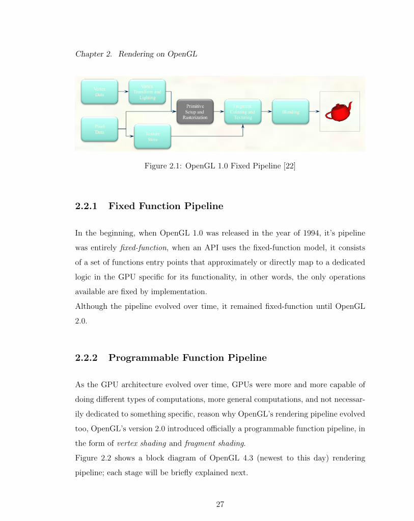
Figure 2.1: OpenGL 1.0 Fixed Pipeline [22]
2.2.1 Fixed Function Pipeline
In the beginning, when OpenGL 1.0 was released in the year of 1994, it’s pipeline
was entirely fixed-function, when an API uses the fixed-function model, it consists
of a set of functions entry points that approximately or directly map to a dedicated
logic in the GPU specific for its functionality, in other words, the only operations
available are fixed by implementation.
Although the pipeline evolved over time, it remained fixed-function until OpenGL
2.0.
2.2.2 Programmable Function Pipeline
As the GPU architecture evolved over time, GPUs were more and more capable of
doing different types of computations, more general computations, and not necessar-
ily dedicated to something specific, reason why OpenGL’s rendering pipeline evolved
too, OpenGL’s version 2.0 introduced officially a programmable function pipeline, in
the form of vertex shading and fragment shading.
Figure 2.2 shows a block diagram of OpenGL 4.3 (newest to this day) rendering
pipeline; each stage will be briefly explained next.
27
Page 44
Chapter 2. Rendering on OpenGL
Figure 2.2: OpenGL 4.3 Rendering Pipeline[7]
• Vertex shading: Receives the vertex data, specified in VBOs, processing each
vertex separately. This stage is mandatory for all OpenGL programs, and must
have a shader bound to it.
• Tessellation shading: This is an optional stage, that generates additional ge-
ometry within the OpenGL pipeline, as compared to having the application
specify each geometric primitive explicitly. This stage receives the output of
the vertex shading stage, and does further processing of the received vertices.
• Geometry shading: This is another optional stage, that can modify the entire
geometric primitives within the OpenGL pipeline, this stage operates on in-
dividual geometric primitives allowing each to be modified, additionally more
28
Page 45
Chapter 2. Rendering on OpenGL
geometry may be generated from the input primitive,change the type of geo-
metric primitive or discarding geometry altogether. It receives its input after
vertex shading has completed processing the vertices of a geometric primitive
or from the primitives generated from the tessellation shading stage.
• Fragment shading: This stage processes the individual fragments generated by
the OpenGL’s rasterizer, it must have a shader bound to it, here a fragment’s
color and depth values are computed and then sent for further processing in
the fragment-testing and blending parts of the pipeline.
• Compute shading: Although it is not part of the graphics pipeline as all the
other stages. A computer shader processes generic work items, driven by an
application-chosen range, rather than by graphical inputs like vertices and frag-
ments. Compute shaders can process buffers created and consumed by other
shader programs in the application.
2.2.2.1 GLSL
It is important to understand what shaders are, they work like a function call, where
data is passed in, some process is applied to the data and then its returned, these
functions are written in the OpenGL Shading Language (GLSL), which is a special
language very similar to C++ used specifically for constructing shaders. Here I will
give a very brief explanation on how to load GLSL shaders.
A GLSL shader is provided in a string of characters, it can either be loaded from a
file of declared as a string of characters on code, most times the first method being
more effective since, those files may be changed after compiling without a problem.
The first line on a shader file must specify the version of GLSL to be used, if it is
not specified GLSL 110 will be assumed and may be incompatible with the current
OpenGL version, just as in C or C++ variables are declared before the declaration
29
Page 46
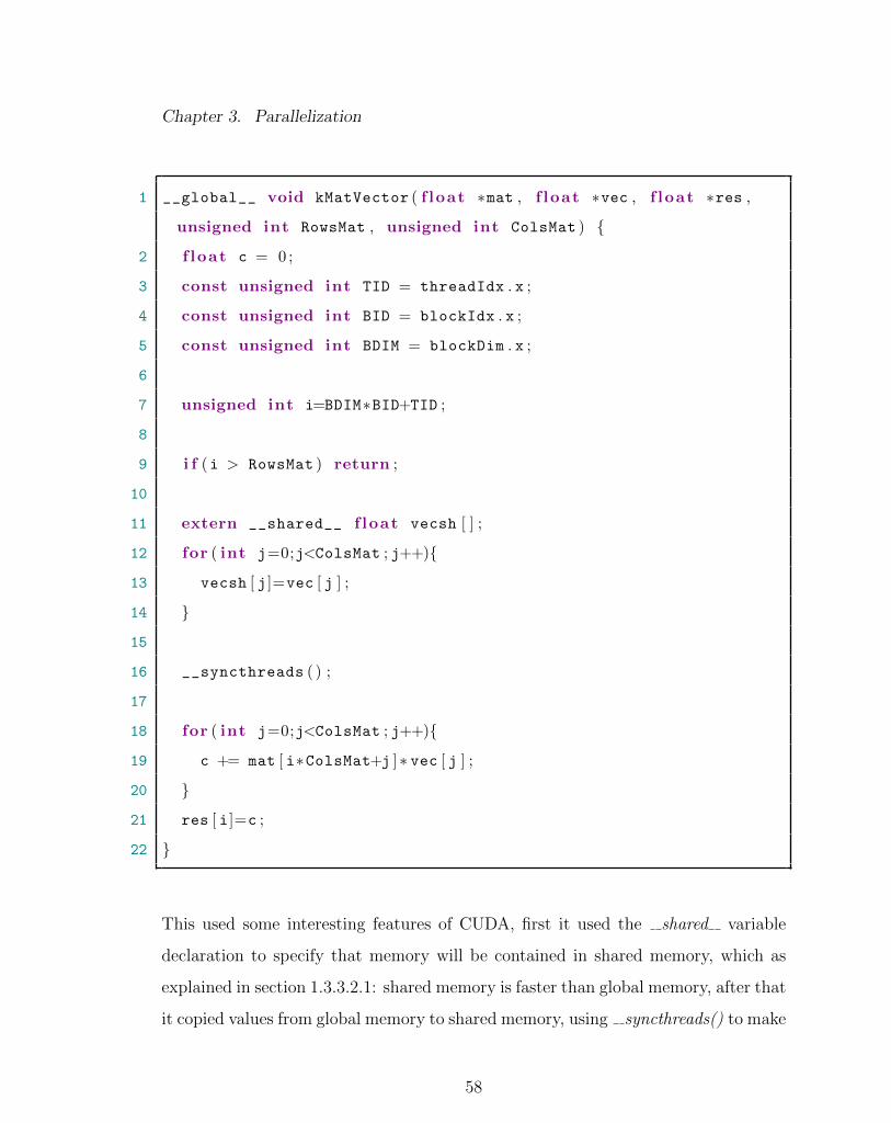
2
Chapter 2. Rendering on OpenGL
of the main() function, these variables are the connection to the outside world, the
shader does not know where its data is coming from but it only sees its input variables
populated with data every time it executes, hence the importance of these shader
variables, if they are not specified correctly the shader won’t be able to do much.
In the main() function is where the shader actually performs calculations using
the variables populated with the input, a good and simple example is passing the
position of a node as the input to the vertex shader, using the vertex shader as a
pass-through shader copying the input to the output, which will; eventually be the
input of the fragment shader, in which in its main() function will perform some cal-
culation and based on the node’s position a different color may be obtained. The
shaders utilized for this work are located in the appendix of this document.
To associate data going into the vertex shader we need to connect the shader vari-
ables declared as ”in” to a vertex attribute array, which will be explained in section
2.3. Shaders also need to be compiled before they are used, they work in a similar
way as C programs, the compiler analyses the program, checking for errors, trans-
lates it into object code, which is then linked to generate an executable program, the
main difference is that the compiler and linker are also part of the OpenGL API.
This process is shown on figure 2.3. To create a shader object, the function glCre-
ateShader() is used as follows:
1 GLuint glCreateShader ( GLenum type ) ;
2 /* Allocates a shader object, type must be one of
3 GL_VERTEX_SHADER , GL_FRAGMENT_SHADER , GL_TESS_CONTROL_SHADER ,
4 GL_TESS_EVALUATION_SHADER , or GL_GEOMETRY_SHADER */
Once the shader object is created it needs to be associated with the source code of
the shader, that is done with the function glShaderSource().
30
3
Page 47
Chapter 2. Rendering on OpenGL
Figure 2.3: Shader compilation process[7]
1 void glShaderSource ( GLuint shader , GLsizei count ,
4 const GLchar ∗∗string , const GLint ∗length ) ;
5 /* Associates the source of a shader with a shader object shader.
6 string is an array of count GLchar strings that compose the
As explained in the figure the next step is to compile the shader object:
1 void glCompileShader ( GLuint shader ) ;
2 /* Compiles the source code for shader. The results of the
3 compilation can be queried by calling glGetShaderiv() with
4 an argument of GL_COMPILE_STATUS. */
After the shader object was compiled, they need to be linked to create an executable
shader program, this is a similar process as the one explained before for creating
31
Page 48
Chapter 2. Rendering on OpenGL
shader objects, first a shader program needs to be created, to be able to attach those
shader objects to it.
1 GLuint glCreateProgram (void ) ;
2 /* Creates an empty shader program. The return value is either
3 a nonzero integer, or zero if an error occurred. */
and to attach shader objects to it:
1 void glAttachShader ( GLuint program , GLuint shader ) ;
2 /* Associates the shader object, "shader" , with the shader
3 program, "program". A shader object can be attached to a shader
4 program at any time, although its functionality will only be
5 available after a successful link of the shader program.
6 A shader object can be attached to multiple shader programs
7 simultaneously. */
A shader object may be removed from a program with:
1 void glDetachShader ( GLuint program , GLuint shader ) ;
2 /* Removes the association of a shader object, "shader", from
3 the shader program, "program". If shader is detached from program
4 and had been previously marked for deletion (by calling
5 glDeleteShader()), it is deleted at that time. */
Now with all the shader objects attached to the program, they need to be linked in
order to become an executable program:
1 void glLinkProgram ( GLuint program ) ;
2 /* Processes all shader objects attached to "program" to generate
3 a completed shader program. The result of the linking operation
4 can be queried by calling glGetProgramiv() with GL_LINK_STATUS.
32
Page 49
Chapter 2. Rendering on OpenGL
5 GL_TRUE is returned for a successful link; GL_FALSE otherwise. */
After a program has been successfully linked it can be used like this:
1 void glUseProgram ( GLuint program ) ;
2 /* Use the linked shader program "program". */
Shader objects and shader programs may be deleted as follows respectively:
1 void glDeleteShader ( GLuint shader ) ;
2 /* Deletes shader. If shader is currently linked to one or more
3 active shader programs, the object is tagged for deletion and
4 deleted once the shader program is no longer being used by any
5 shader program. */
1 void glDeleteProgram ( GLuint program ) ;
2 /* Deletes program immediately if not currently in use in any
3 context, or schedules program for deletion when the program is
4 no longer in use by any contexts. */
2.3 Buffer Objects
Buffers objects are general purpose memory storage blocks allocated by OpenGL,
they give OpenGL implementations flexibility and improve performance, although
they are generic by definition, the programmer is required to specify or describe the
usage for them during the implementation, they can be used to store many types of
data, but in this work buffers are used for storing vertex information, hence they are
called Vertex Buffer Objects (VBOs).
33
Page 50
Chapter 2. Rendering on OpenGL
To allocate data on a buffer object, a buffer object first need to be created, this is
done using the glGenBuffers() command, and it has the following prototype:
1 void glGenBuffers ( GLsizei n , GLuint ∗buffers ) ;
2 /* Returns n currently unused names for buffer
3 objects in the array buffers. */
This will create an array of buffer objects names located at &buffers, although they
are not object buffers yet, they are only placeholders. The buffer objects are not
created until the name is bound to one of the buffer binding points on the con-
text. There are several types of buffer binding points or also called targets, such
as: GL ARRAY BUFFER for VBOs and GL ELEMENT ARRAY BUFFER for El-
ement Buffer Objects, which is where the vertex indices are contained.
Buffer objects will be actually created after the binding is done, using the glBind-
Buffer() command, with the following prototype:
1 void glBindBuffer ( GLenum target , GLuint buffer ) ;
2 /* Binds the buffer object "buffer" to the specified
3 buffer binding point as specified by "target". */
After creating the buffer, the next step to make something useful out of it, is to put
data on it. This is done via the glBufferData() function:
1 void glBufferData ( GLenum target , GLsizeiptr size ,
2 const GLvoid ∗data , GLenum usage ) ;
3 /* Allocate size bytes of storage for the object bound
4 to the target, data must be non-null, usage describes
5 the intended usage for that buffer */
The function glBufferData() allocates storage, if size is larger than the space allo-
cated for that buffer, the buffer will be resized, it is important to note the usage
34
Page 51
Chapter 2. Rendering on OpenGL
parameter, since it may have big influence on the performance of the program, it
should be specified as one of the OpenGL usage tokens.
These usage tokens are composed of 2 parts: The first one can be either STATIC,
DYNAMIC, STREAM, while the second one can be DRAW, READ or COPY, these
are explained in further detail in table 2.3. OpenGL will make decisions based on
STATIC Contents will be modified once and used manytimes.
DYNAMIC Contents will be modified repeatedly, and usedmany times.
STREAM Contents will be modified once and used at mosta few times.
DRAW Contents are modified by the application and usedas the source for OpenGL drawing and image spec-ification commands.
READ Contents are modified by reading data fromOpenGL and used to return that data whenqueried by the application.
COPY Contents are modified by reading data fromOpenGL and used as the source for OpenGL draw-ing and image specification commands.
Table 2.1: Buffer Usage Tokens [7]
this parameter, such as placing the data on fast memory or avoiding to do so, if
considers it not convenient.
To modify a buffer, completely or partially, the function glBufferSubData() is used
like this:
1 void glBufferSubData ( GLenum target , GLintptr offset ,
2 GLsizeiptr size , const GLvoid ∗data ) ;
3 /* Replaces a subset of a buffer object’s data store
4 with new data. The section of the buffer object bound
5 to "target" starting at "offset" bytes is updated with
35
Page 52
Chapter 2. Rendering on OpenGL
6 "size" bytes of data addressed by "data". */
When the buffers are correctly populated with the required data, this data needs
to be hooked up to the shader. Vertex Array Objects (VAOs) are OpenGL objects
that describe how the vertex attributes are stored in a Vertex Buffer Object (VBO),
the VAO is not the object storing the vertex data but it is only the descriptor
of this data. To associate the data going into the vertex shader, the shader ”in”
variables need to be connected to a Vertex Attribute Array, doing so with the function
glVertexAttribPointer():
1 void glVertexAttribPointer ( GLuint index , GLint size , GLenum type ,
2 GLboolean normalized , GLsizei stride , const GLvoid ∗pointer ) ;
3 /* Specifies where the data values for the vertex attribute with
4 location "index" can be accessed. "pointer" is the offset in
5 bytes from the start of the buffer object currently bound to the
6 GL_ARRAY_BUFFER target for the first set of values in the array.
7 "size" represents the number of components to be updated per
8 vertex. "type" specifies the data type of each element in the
9 array. "normalized" indicates that the vertex data should be
10 normalized before being presented to the vertex shader. "stride"
11 is the byte offset between consecutive elements in the array. */
The state set by this function is stored in the currently bound VAO, there is only
one thing left to do to be able to use this data, the VAO needs to be enabled, and
this is done by the function glEnableVertexAttribArray():
1 void glEnableVertexAttribArray ( GLuint index ) ;
2 void glDisableVertexAttribArray ( GLuint index ) ;
3 /* Specifies that the vertex array associated with variable index
4 be enabled or disabled. index must be a value between zero and
36
Page 53
Chapter 2. Rendering on OpenGL
5 GL_MAX_VERTEX_ATTRIBS 1. */
Once the data is ready to be used by OpenGL, all that needs to be done is draw it
on the screen, for this the function glDrawElements() will be used.
1 void glDrawElements ( GLenum mode , GLsizei count ,
2 GLenum type , const GLvoid ∗indices ) ;
3 /* Defines a sequence of geometric primitives using "count"
4 number of elements, whose indices are stored in the buffer bound
5 to the Element Array Buffer (EAB). "indices" represents an offset
6 ,in bytes, into the EAB where the indices begin. "type" must be
7 one of GL_UNSIGNED_BYTE , GL_UNSIGNED_SHORT , or GL_UNSIGNED_INT ,
8 indicating the data type of the indices the EAB. "mode" specifies
9 what kind of primitives are constructed. */
2.4 External Libraries
2.4.1 GLUT
As explained before, OpenGL is designed to be implemented on different hardware
and it is independent of the operating system running on the computer, for this very
reason, OpenGL does not contain any functions or commands to manage windows,
this needs to be done manually depending on the operating system the software is
intended to run on, in this work the GLUT (OpenGL Utility Toolkit) library was
used to overcome this, facilitating the OpenGL initialization and window managing.
The version of GLUT used is called freeglut, it is based on the original version, but
it’s more updated and more compatible in many cases, a more in depth explanation
37
Page 54
Chapter 2. Rendering on OpenGL
of how GLUT works can be found at [23].
GLUT makes making OpenGL applications a simpler process, this is done in its most
basic form in the following way:
• Initialization: In the initialization part several functions are called, such as
glutInit(), and glutCreateWindow(), their names are very obvious of what they
do, but also in this phase other functions may be called, to specify the window
size, position or OpenGL display mode for example.
• Registering Callbacks: In this phase, the programmer must specify the func-
tions that will be called when a specific event happens, this functions could be
for example, what function to call when a key was pressed or released on the
keyboard (glutKeyboardFunc()), when the user uses a mouse button or even
moves the mouse(glutMouseFunc() and glutMotionFunc()), and some of them
more needed than others, such like what function to call when it’s time to
display or render something on the screen (glutDisplayFunc()), when OpenGL
is idle (glutIdleFunc()), or when the window is resized(glutReshapeFunc()).
• Main Loop: Lastly what needs to be done is to call the glutMainLoop() function
which basically loops between the functions previously specified and has an
event handler to perform the correct callback for a specific event.
2.4.2 GLEW
GLEW is the OpenGL Extension Wrangler, which is another external library used in
this work, it is a cross platform open source C/C++ extension loading library, GLEW
provides efficient runtime mechanisms for determining which OpenGL extensions
are supported on the target platform, OpenGL core and extension functionality is
38
Page 55
Chapter 2. Rendering on OpenGL
exposed in a single header file glew.h, all that needs to be done is to initialize it
calling the function glewInit() after creating the window using GLUT[].
2.4.3 GLM
OpenGL Mathematics or GLM is a header only c++ mathematics library for graph-
ics software based on the OpenGL Shading Language (GLSL), this library intends
to provide classes and functions designed and implemented following as strictly as
possible the GLSL conventions and functionalities so that when a programmer knows
GLSL, GLM will also look familiar, although it is not limited to GLSL, it provides
extended capabilities including matrix transformations, quaternions, random number
generation, among others, it also ensures interoperability with third party libraries
, SDKs and OpenGL, it replaces deprecated functions, and as a general purpose
library it can be used in many applications. In this work the GLM library is used
primarily to perform the object manipulations using matrices for transformations
and rotations, and camera manipulation.
39
Page 56
Chapter 3
Parallelization
When using parallel computing to develop parallel algorithms it is a good idea to
follow some software engineering discipline or programming model, one good example
is the APOD (Analyze Parallelize Optimize and Deploy) model, which is defined as
a systematic automation process, that the programmer must follow to break down
the optimization process and succeeding not only at developing fast algorithms, but
also be efficient and organized about it.
First an explanation of the theory behind the algorithm will be explained
3.1 Modal Warping
This work is based primarily on the paper presented at the IEEE transactions on
visualization and computer graphics by Min Gyu Choi and Hyeong-Seok Ko [5].
In their work they present a technique to perform real time simulation of objects,
their work is based on implementing a special type modal analysis called modal
warping to FEM to improve simulation speed when using large objects, however what
40
Page 57
Chapter 3. Parallelization
modal warping fails to achieve is being accurate for large deformations, extending
their modal analysis work to identify a rotational component of an infinitesimal
deformation and being able to keep track of it, achieving accurate results.
Reason why modal analysis is a good choice of algorithm to be implemented on
a GPU; it provides accurate results and applying modal analysis to FEM, as its
explained further in the next section makes it easy to decouple the calculation of the
modal amplitudes making every calculation independent from each other fitting for
the most part the threads organization used in GPGPU computing.
3.1.1 Rotational Part in a Small Deformation
The non-linear term in a strain sensor is the one responsible for the appearance and
disappearance of rotational deformations, since it is generally known that every in-
finitesimal deformation can be decomposed into a rotation followed by a strain this
serves as a basis for this technique, basically: at every timestep of the simulation,
small rotations are identified on every point of the material, then the effect of them
is integrated to obtain the deformed shape.
A brief explanation of this calculation goes as follows:
3.1.1.1 Kinematics of Infinitesimal Deformation
Given an elastic solid object; x ∈ R3 denotes the position of a material node/point
in an undeformed state, which will in turn move to a new position given by a(x) due
to a subsequent deformation.
a(x) = x+ u(x), x ∈ Ω
41
Page 58
Chapter 3. Parallelization
where Ω is the domain of the solid.
Differentiating both sides with respect to x gives us:
da = (I + Ou)dx (3.1)
The infinitesimal strain tensor ε which measures the change in the squared length
of dx during an infinitesimal deformation is defined as:
ε =1
2(Ou+ OuT )
if we note that 12(Ou+ OuT ) is a meaningful quantity, Ou can be decomposed as:
Ou =1
2(Ou+ OuT ) +
1
2(Ou− OuT ) = ε+ ω (3.2)
The skew-symmetric tensor ω, is closely related to the curl of the displacement field
Ou and it may rewritten as:
ω =1
2(Ou− OuT ) =
1
2(O× u)× = w× (3.3)
Where w× denotes the standard skew symmetric matrix of vector w. Therefore
12(O × u)× can be viewed as a rotation vector that causes rotation of the material
points at and near x, by an angle given by θ = ‖w‖ about the unit axis w = w‖w‖
ω is called the infinitesimal rotation tensor
Finally if we substitute equations 3.3 and 3.2 into 3.1 we obtain:
da = dx+ εdx︸︷︷︸+ θw × dx︸ ︷︷ ︸ (3.4)
Showing that an infinitesimal deformation can be decomposed correctly into strain
and rotation.
42
Page 59
Chapter 3. Parallelization
3.1.1.2 Extended Modal Analysis
The purpose of extending the modal analysis is to keep track of the rotation experi-
enced by each material point during deformation.
The governing equation for a finite element model is given by:
Mu+ Cu+Ku = F (3.5)
Where u(t) is a 3n-dimensional vector representing the displacements of the n nodes,
from their original positions and F (t) is a vector that represents the external forces
acting on the nodes. The mass, damping and stiffness matrices M, C and K respec-
tively are independent of time and are completely characterized at the rest state
under the commonly adopted assumption that C = ξM + ζK where ξ and ζ are
scalar weighting factors (Rayleigh Damping) [5].
In general M and K are not diagonal, thus equation 3.5 is a coupled system of ordi-
nary differential equations (ODEs). Let Φ and a diagonal matrix Λ be the solution
matrices to the generalized eigenvalue problem: KΦ = MΦΛ, such that ΦTMΦ = I
and ΦTKΦ = Λ.
Since the columns of matrix Φ form a basis of the 3n-dimensional space, u can be
expressed as a linear combination of the columns:
u(t) = Φq(t) (3.6)
Where Φ is the modal displacement matrix ; every column represents a different mode,
and q(t) is a vector containing the corresponding modal amplitudes.
Examining the eigenvalues, allows to only take dominant columns (modes) of Φ, re-
ducing significantly the amount of computation to be performed.
Substituting equation 3.6 in equation 3.5 followed by a premultiplication of ΦT de-
couples 3.5 as:
Mq q + Cq q +Kqq = ΦTF (3.7)
43
Page 60
Chapter 3. Parallelization
where Mq = I , Cq = ξI + ζΛ, and Kq = Λ are now all diagonal matrices and ΦTF
is defined as the modal force.
Manipulating the previous equation the following equations can be obtained:
qk =(α− I) ∗ qk−1 + β ∗ qk−1 + γ ∗ ΦT ∗ F k−1
h(3.8)
qk = α ∗ qk−1 + β ∗ qk−1 + γ ∗ ΦT ∗ F k−1 (3.9)
Where h is the time step size and the coefficient matrices can be obtained by:
αi = 1− h2 ∗ kidi
βi = h ∗ (1− h ∗ Ci + h2 ∗ kidi
)
γi =h2
di
di = Mi + h ∗ Ci + h2 ∗ ki
Where: Mi, Ci and Ki represent the diagonal entries of Mq,Cq and Kq
3.1.1.3 Modal Rotation
While the conventional way of accurately calculating strain and deformation is de-
fined as:
ε = Ou ∗ OuT (3.10)
The previous equation provides accurate results but it is computationally complex,
reason why it is chosen to use the infinitesimal strain sensor from equation 3.3,
trading off accuracy for complexity, to overcome this problem the calculation of
displacement for every node needs to be independent of rotation, and the rotation
44
Page 61
Chapter 3. Parallelization
must be included afterwards.
The rotation matrix is defined as follows:
R =
∫ t
0
ω(t) ∗ dt (3.11)
Where ω(t) is the angular velocity of a certain node for in a specific timestep.
It can be assumed that the rotation linearly varies from 0 to t starting at 0 and ending
in w, for a certain time w∗τt→ R, given this we can include define the composite
vector w(t) as follows:
w(t) = W ∗ Φ ∗ q(t) = Ψ(q(t) (3.12)
To make the calculation time independent Ψ can be defined as and be precomputed
as:
Ψ = W ∗ Φ (3.13)
Equation 3.12, will later be used to calculate the rotation using Rodrigues formula
[24]
Ri = [I + (wi×)1− cos‖wi‖‖wi‖
(wi×)2(1− sin‖wi‖‖wi‖
)] (3.14)
Where: i indicates this calculation is for a specific node , wi× is defined as the
skew symmetric matrix for that specific node and ‖wi‖ is the magnitude of the skew
symmetric matrix and I is the identity matrix with a size of n ∗ n, given that it is a
3 dimensional node n = 3, and finally Ri will also be a n ∗ n matrix.
Lastly what needs to be done is to include the rotational part in the displacement
calculation doing so by applying Ri on equation 3.6 for a specific node:
ui(t) = Ri ∗ ui(t) (3.15)
After doing so u(t) will contain not only displacement information for all nodes but
also rotation information, which will only need to be applied to the nodes original
location to get the new location for a specific timestep.
45
Page 62
Chapter 3. Parallelization
3.1.2 Implementation
The implementation of the modal warping technique will be explained in this section.
The displacement is given by equation 3.6, it is obtained by the multiplication of
the modal displacement matrix by the vector containing the corresponding modal
amplitudes, to get these two elements, we need to solve the eigen problem first to get
Φ; which in this case its precomputed and use equations 3.8 and 3.9 to obtain q.
Lastly using equation 3.14 we can also include the rotational information, providing
an accurate result.
A brief analysis of the equations previously will give the chronological order in which
the elements need to be obtained: The final goal is to obtain a displacement per
3-dimensonal node, which is given by:
u(t) = Φq(t)
To obtain u first Φ and q need to be obtained, in the case of Φ it is assumed it was
previously computed, and q will be given by the following equation:
qk = α ∗ qk−1 + β ∗ qk−1 + γ ∗ ΦT ∗ F k−1
Asit can be seen to get q we not only need to get q first using equation:
qk =(α− I) ∗ qk−1 + β ∗ qk−1 + γ ∗ ΦT ∗ F k−1
h
But also the coefficients matrices which are given by:
αi = 1− h2 ∗ kidi
βi = h ∗ (1− h ∗ Ci + h2 ∗ kidi
)
γi =h2
di
46
Page 63
Chapter 3. Parallelization
di = Mi + h ∗ Ci + h2 ∗ ki
Where: Mi, Ci and Ki represent the diagonal entries of Mq,Cq and Kq, and as
explained in section 3.1 we can assume that K contains the eigenvalues, M is the
Identity matrix and C is a linear combination of both. In chronological order of
execution, calculations need to be performed as follows:
1. Solve the Eigenproblem: From this: Φ and K will be obtained, being the
eigenvectors and the eigenvalues respectively.
2. Compute C : After getting K and knowing that M is the Identity matrix, C
can be computed as a linear combination of both.
3. Compute Coefficient Matrices: All the coefficient matrices will be diagonal
matrices obtained from the equations previously explained.
The elements previously mentioned are time independent and can be computed at
the beginning of the program, while the following need to be computed at every
timestep or iteration of the program:
1. Compute q
2. Compute q
3. Compute u
4. Compute rotation: rotational information needs to be calculated, and it can
be obtained using the Rodrigues’s formula
5. Include rotation: Including the rotational information obtained in the last
element is vital since it will give an accurate result
47
Page 64
Chapter 3. Parallelization
3.2 Analyze Stage
The first step of the model is to analyze the problem, or in this case analyze the cur-
rent algorithm, which was developed using conventional computing, executing CPU
code exclusively, the original algorithm was developed using MATLAB as stated be-
fore, so the first step was to create or translate the original algorithm from MATLAB
to C/C++, doing so to not only to get a better performance already, but also to be
able to reuse parts of this code on the parallel version programmed in CUDA.
3.2.1 GNU Profiler
A good way of analyzing a program is using a technique called profile based analysis,
profiling an application will output some vital information of where the program
spends its time, and this in turn will facilitate developing algorithms that will improve
performance on the parts of the code where its most important, GNU profiler (gprof)
was the tool selected to do this task [25]. Below is the filtered output of the GNU
profiler:
1 $ gprof −p mwgpu
2
3 % cumulative self self total
4 time seconds seconds calls ms/call ms/call name
5 83 .01 1 .71 1 .71 135378 0 .01 0 .01 matrixByVec ( . . . )
6 8 .25 1 .88 0 .17 414 0 .41 0 .41 matrixTranspose ( . . . )
7 3 .88 1 .96 0 .08 132480 0 .00 0 .00 matrixMult ( . . . )
8 3 .40 2 .03 0 .07 414 0 .17 0 .17 insertZeros ( . . . )
9 0 .49 2 .05 0 .01 1656 0 .01 0 .01 vectorAdd ( . . . )
Listing 3.1: GNU Profiler Filtered Output
48
Page 65
Chapter 3. Parallelization
From this output we can see easily in what functions the program spends more
time, it is important to also note the amount of times a certain function was called,
since noticing that a programs spends a lot of time on a certain function might not
necessarily mean its inefficient, it might be that it just needs to call that function a
lot of times.
As noted before the functions where the program spends more time are, in order of
time spent:
• matrixByVec()
• matrixTranspose()
• matrixMult()
• insertZeros()
• vectorAdd()
• computeR()
This is valuable information, since it gives a good start point on where the paral-
lelization would improve more the original algorithm, after getting this information,
singling out every one of this functions to analyze is the next step.
After analyzing all the functions, it can be stated that the functions matrixByVec(),
matrixTranspose() and matrixMult() can be parallelized in most of their computa-
tions, while insertZeros() and computeR() not so much, but since most of the time
spent is on the first three functions mentioned, it can be presumed that a good
optimization will be achieved.
49
Page 66
Chapter 3. Parallelization
3.2.2 Amdahl’s Law
To be able to approximate the performance gain that can be obtained by improving
some portion of an algorithm may be improved, Amdahl’s Law is used. Amdahl’s
law states that the performance improvement to be gained from using some faster
mode of execution is limited by the fraction of time the faster mode can be used.
Amdahl’s law defines the speedup that can be gained by using a particular feature[8].
Where speedup is defined as:
Speedup =Performance using the enhancementwhen possible
Performancewithout using the enhancement(3.16)
Amdahl’s law gives a quick way to find the speedup from some enhancement, depend-
ing on two factors: The fraction of the computation time in the original algorithms
that can be converted to take advantage of the enhancement, and the improvement
gained by the enhanced execution mode (how much faster the task would run if the
enhanced mode where to be used for the entire algorithm. The execution time is
defined as follows:
ExecT imenew = ExecT imeold ∗ ((1−Fractionenhanced)+FractionenhancedSpeedupenhanced
) (3.17)
and the overall speedup is the ration of the execution times:
Speedupoverall =ExecT imeoldExecT imenew
(3.18)
or:
Speedupoverall =1
((1− Fractionenhanced) + Fractionenhanced
Speedupenhanced)
(3.19)
Amdahl’s law expresses the law of diminishing returns: The incremental improvement
is the speedup gained by an improvement of just a portion of the computation, it
diminishes as improvements are added. Analyzing the specific case of this algorithm
we can note that the fraction of the code that can be improved is a constant, where
50
Page 67
Chapter 3. Parallelization
this fraction was approximated using the profiler in section 3.2.1, although the time
spent on executing it’s a variable, depending on how large the object used on the
simulation is, the number of nodes the object has and the number of eigenvalues used
in the calculation, will define the time spent on calculating the modal displacement.
It can be presumed then that as the object gets larger and larger, the gain on
algorithm performance will also increase.
3.2.3 Computer and device specs
It is also important to specify the specifications of the devices and software used to
measure performance improvement, these will be described in the following listings:
1 OS : Arch Linux x86_64 GNU/Linux
2 Kernel : 3.14.0−5−ARCH
3
4 GCC : gcc ( GCC ) 4 . 8 . 2 20140206 ( prerelease )
5
6 Make : GNU Make 4 .0
7
8 NVCC : NVIDIA (R ) Cuda compiler driver
9 Cuda compilation tools , release 6 . 0 , V6 . 0 . 1
Listing 3.2: Operating System & Software Specifications
The CPU and system memory specifications are a filtered version of the information
taken from the files /proc/cpuinfo and /proc/meminfo, gotten using the Linux kernel,
and some information using other commands.
51
Page 68
15
Chapter 3. Parallelization
1 Processor : Genuine Intel (R ) Core 2 Duo CPU U7300 @ 1 .30 Ghz
2 CPU MHz : 1733 .00
3 Cache Size : 3072 KB
4
5 Memory :
6 Size : 4096 MB
7 Form Factor : SODIMM
8 Type : DDR3
9 Speed : 800 MHz
Listing 3.3: CPU and System Memory Specifications
GPU or device specifications listed below are a filtered version of the output obtained
by the deviceQuery utility given by NVIDIA with the CUDA release, and also the
information obtained using the NVIDIA Visual Profiler [26], whose functionality will
be explained in section 3.4.
1 GPU : GeForce GT 335M
2 CUDA Driver Version / Runtime Version 6 .0 / 5 .5
3 CUDA Capability Major/Minor version number : 1 . 2
4 Total amount of global memory : 1023 MBytes
5 ( 9) Multiprocessors , ( 8) CUDA Cores/MP : 72 CUDA Cores
6 GPU Clock rate : 1080 MHz
7 Memory Clock rate : 790 Mhz
8 Memory Bus Width : 128−bit
9 Warp size : 32
10 Maximum number of threads per multiprocessor : 1024
11 Maximum number of threads per block : 512
12 Max dimension size of a thread block (x , y , z ) : (512 , 512 , 64)
13 Max dimension size of a grid size (x , y , z ) : (65535 , 65535 , 1)
52
16
Page 69
Chapter 3. Parallelization
14 Integrated GPU sharing Host Memory : No
17 Support host page−locked memory mapping : Yes
18 Device supports Unified Addressing ( UVA ) : No
Listing 3.4: GPU Specifications
The above is perhaps the most valuable information of all, since as specified before
in section 1.3.3.2, when using parallel computing on the GPU; the programmer must
develop algorithms somewhat based on the underlying architecture of the device,
for example the amount of maximum threads possible to execute per block is a
very important parameter, which was thought of when developing the algorithm, or
another important parameter would be the amount of CUDA cores available for a
specific device.
3.3 Parallelize Stage
With all the information previously obtained, CUDA can be integrated to an existing
C/C++ application, the CUDA entry point being a host only function, containing
the kernel or kernels, called from C/C++ code.
The compiler needed for CUDA code is called nvcc, and it only needs to compile
the file that contains the function previously specified, while any other file can be
compiled with a conventional compiler such as gcc. First, a host only function was
created called displacement(), parameters such as the force vector, number of nodes,
eigenvalues, among others were passed to it, the purpose of this function as mentioned
before was to be a entry point to CUDA, in this function the environment to use
CUDA is created, allocating GPU memory, copying memory from host to device or
vice-versa, calculating the amount of threads needed to be run per block (there is a
53
Page 70
Chapter 3. Parallelization
maximum amount of threads depending on the device), etc. Although once all that
is done this function is also in charge of one of the most important things, which is
launching the kernels.
To implement the parallel algorithm the same ”sequence” found on the conventional
algorithm was followed, creating a parallel version of the functions needed, as it was
shown before the most important ones were matrixByVec(), matrixTranspose(), etc.
These functions were ”replicated” in the form or kernels.
In this first version the displacement() function would be called from inside the
OpenGL loop created by GLUT [23], it would allocate and copy all the memory
needed on the GPU, launch the kernels to perform different calculations, and after
a result for that node displacement was obtained it would return that result in the
form of an array which would then be used in the main code to modify the OpenGL
buffer previously created, to render the object on the screen.
3.3.1 Kernel Development
In this section a basic explanation of the kernels developed will be given.
The major kernels used in this work as it was shown in figure 3.3 are:
• kMatVector
• kInsertZeros
• kVectorAdd
• kModBuffer
• kComputeR
54
Page 71
Chapter 3. Parallelization
These kernels are used to implement the equations found on section 3.1.2, the purpose
of these equations is to be able to get the location displacement from every node
contained on the object, while keeping the rotation information too.
The calculations that need to be parallelized are the ones to be computed on every
iteration of the program, hence obtaining a better improvement in performance.
Analyzing the following equation the q vector can be obtained:
qk =(α− I) ∗ qk−1 + β ∗ qk−1 + γ ∗ ΦT ∗ F k−1
h
It can be separated in 5 main operations:
result1 = (α− I) ∗ qk−1
result2 = β ∗ qk−1
result3 = γ ∗ ΦT ∗ F k−1
result = Σni resulti
q =result
h= result ∗ 1
h
• The first part (result1) can also be separated in an addition between matrices
(α + (−Identity)) multiplied by qk−1 which is a vector.
• The second part (result2) is merely a matrix (β) multiplication by a vector
(qk−1).
• The third part (result3) performs two sequential multiplications, the first one
a matrix by a vector ΦT ∗ F k−1 assuming that the transpose of Φ was previ-
ously calculated, and the second one, multiplying the result obtained by the
coefficient matrix γ.
55
Page 72
Chapter 3. Parallelization
• The next operation is to perform an addition of the result obtained from all
the previous ones.
• And the last one is to multiply that result which is a vector by a scalar ( 1h).
With the next equation q can be obtained:
qk = α ∗ qk−1 + β ∗ qk−1 + γ ∗ ΦT ∗ F k−1
Looking at the previous equation, it can be seen that it could be separated in the
following operations:
result1 = (α) ∗ qk−1
result2 = β ∗ qk−1
result3 = γ ∗ ΦT ∗ F k−1
q = Σni resulti
But looking closely, two of these operations were already calculated previously to get
q (β ∗ qk−1 and γ ∗ΦT ∗F k−1), so the only one different is (α) ∗ qk−1 and then adding
them all together. This will take more space in memory but save time not performing
unnecessary calculations. With these results now the following calculation can be
computed:
u(t) = Φq(t)
This is again a matrix (Φ) multiplication by a vector (q(t))
After this the only computation needed is to include the rotational information in
vector u(t) although it is not that simple, to do this we need to implement equation
3.15:
ui(t) = Ri ∗ ui(t)
56
Page 73
Chapter 3. Parallelization
This will include the rotation information in the u(t) but it will do it for every node,
the Ri matrix can be obtained using Rodrigues’s formula like this:
Ri = [I + (wi×)1− cos‖wi‖‖wi‖
(wi×)2(1− sin‖wi‖‖wi‖
)]
To implement this the following calculations need to be performed first:
1. Compute w vector
2. Compute wi skew symmetric matrix
3. Calculate wi vector’s norm
4. Calculate the skew symmetric matrix squared: wi×2
Vector w(t) can be obtained by multiplying the Ψ matrix by vector q(t), where it is
assumed that this matrix was previously precomputed.
And the skew symmetric matrix of vector wi is given by:
0 −w3 w2
w3 0 −w1
−w2 w1 0
.
Generic kernels were created to perform matrix and vector operations, it was decided
this way instead of creating one major kernel to perform calculations per element
because the device available was not powerful computationally speaking.
After several tests and performance measurements it was proven that using generic
kernels was more efficient for this device while the same code could still work on
better devices.
A good example of this is the kmatrixByVec kernel which performs the multiplication
of a matrix by a vector, the original code developed was this:
57
Page 74
Chapter 3. Parallelization
1 __global__ void kMatVector ( f loat ∗mat , f loat ∗vec , f loat ∗res ,
unsigned int RowsMat , unsigned int ColsMat )
2 f loat c = 0 ;
3 const unsigned int TID = threadIdx . x ;
4 const unsigned int BID = blockIdx . x ;
5 const unsigned int BDIM = blockDim . x ;
6
7 unsigned int i=BDIM∗BID+TID ;
8
9 i f (i > RowsMat ) return ;
10
11 extern __shared__ f loat vecsh [ ] ;
12 for ( int j=0;j<ColsMat ; j++)
13 vecsh [ j ]=vec [ j ] ;
14
15
16 __syncthreads ( ) ;
17
18 for ( int j=0;j<ColsMat ; j++)
19 c += mat [ i∗ColsMat+j ]∗ vec [ j ] ;
20
21 res [ i ]=c ;
22
This used some interesting features of CUDA, first it used the shared variable
declaration to specify that memory will be contained in shared memory, which as
explained in section 1.3.3.2.1: shared memory is faster than global memory, after that
it copied values from global memory to shared memory, using syncthreads() to make
58
Page 75
Chapter 3. Parallelization
sure all threads were synchronized and the vector in shared memory contained all
the information needed, after that the actual matrix by vector multiplication was
calculated, nonetheless performance was slow and the code had to be modified to:
1 __global__ void kMatVector ( f loat ∗mat , f loat ∗vec , f loat ∗res ,
unsigned int RowsMat , unsigned int ColsMat )
2 f loat c = 0 ;
3 const unsigned int TID = threadIdx . x ;
4 const unsigned int BID = blockIdx . x ;
5 const unsigned int BDIM = blockDim . x ;
6
7 unsigned int i=BDIM∗BID+TID ;
8
9 for ( int j=0;j<ColsMat ; j++)
10 c += mat [ i∗ColsMat+j ]∗ vec [ j ] ;
11
12 res [ i ]=c ;
13
Getting rid of all shared memory operations.
The architecture on this device was not able to hold enough shared memory for
the vector in some of the models, and while a workaround could have been found
for this, the processors were still too slow and sacrificing the use of another for loop
to use shared memory, creating another branch in the thread code was simply not
feasible.
Two other important kernels used were the kModBuffer and kVectorAdd, which as
the name suggests, the first one modifies the OpenGL graphics buffer and the second
59
Page 76
Chapter 3. Parallelization
one adds two vectors, these two kernels basically perform the same operation since
the graphics buffer is nothing more than a vector in memory. Again shared memory
operations had to be avoided:
1 __global__ void kModBuffer ( f loat ∗buffer , f loat ∗d_nodes , f loat
∗u , unsigned int totalThreads )
2
3 const unsigned int TID = threadIdx . x ;
4 const unsigned int BID = blockIdx . x ;
5 const unsigned int BDIM = blockDim . x ;
6
7 unsigned int index=BDIM∗BID+TID ;
8
9
10 i f ( index>totalThreads )
11 return ;
12 // Add displacement to original nodes
13 buffer [ index ]=d_nodes [ index ]+u [ index ] ;
14
15
The first part of the kernel is to know which thread is actually being executed, this
is how the index for the memory location to be modified is obtained. The if branch
is to make sure the that none of the threads will try to modify memory locations not
part of the buffer, as explained before this was part of the warp optimizations.
While these two kernels seem very simple, they are executed many times hence their
importance on performance.
60
Page 77
Chapter 3. Parallelization
Lastly another important kernel to mention is the kInsertZeros kernel, this is
particularly important because along with the kComputeR kernel its one of the less
parallelizable parts of the program, in fact to be able to do this in parallel it has to
be executed several times, unlike the serial version which is able to do it in only one
execution.
1 __global__ void kInsertZeros ( f loat ∗Input , f loat ∗Output ,
unsigned int position , unsigned int number , unsigned int
numElements )
2 //Get element to work on
3 const unsigned int TID = threadIdx . x ;
4 const unsigned int BID = blockIdx . x ;
5 const unsigned int BDIM = blockDim . x ;
6
7 unsigned int i=BDIM∗BID+TID ;
8 //Array wil be increasin its size per execution
9 i f (i<numElements )
10 // Do it 3 times
11 // i for insert 0’s
12 i f (i>position−1 && i<=position+number−1)
13 Output [ i ]=0;
14 // i After 0’s
15 else i f (i>=position+number )
16 Output [ i ]=Input [ i−number ] ;
17 // i before 0’s
18 else i f (i<position )
19 Output [ i ]=Input [ i ] ;
20
21
61
Page 78
Chapter 3. Parallelization
This kernel inserts three 0’s on the array containing the displacement, each zero
corresponds to a dimension (x,y,z), this is because some of the nodes of the object
are fixed to analyze the object’s behavior, meaning that these nodes should not have
a displacement, and since they are not used for the calculation, these locations in
memory need to be 0. The complex part here is that since it is being done in parallel,
there is no communication between the threads, the programmer cannot know the
order in which threads will be executed, and for this specific operation order does
matter, this is why this kernel needs to be executed several times. It is important to
note that a workaround for this is to use sparse structures which is one of the items
on future work to improve performance of this program.
The kComputeR kernel is very long but some important parts will be explained here,
this kernel implements the Rodrigues’s formula shown in equation 3.14, and it then
includes this information on vector u(t) it is not very parallelizable with the CUDA
version compatible with this device.
1 f loat sum=0;
2 // Compute Norm
3 for (j=0;j<size ; j++)
4 sum+=d_w [ rI+j ]∗ d_w [ rI+j ] ;
5
6 i f (sum<0.00001)
7 norm=1;
8 else
9 norm=sqrtf ( sum ) ;
This part is used to obtain the norm of the vector w, avoiding a future division by
zero, although it is a simple operation, but the usage of sqrt which is unavoidable
makes it slow.
This kernel has to work per node, meaning that unlike most other kernels that
62
Page 79
Chapter 3. Parallelization
perform operations per location in memory, this one perform operations on three lo-
cations of memory, since every node contains information about its three dimensions.
Using CUDA 6 a kernel is able to launch more kernels, which could avoid this and
make every kernel to work on only one location per memory.
1 // Get skew matrix ^2
2 for (j=0;j<size ; j++)
3 for (k=0;k<size ; k++)
4 sum=0;
5 for (l=0;l<size ; l++)
6 sum+=skew_w [ j∗size+l ]∗ skew_w [ l∗size+k ] ;
7
8 skew_w2 [ j∗size+k ]=sum ;
9
10
11
12 // Get R Matrix
13 for (j=0;j<size∗size ; j++)
14 R [ j ]=Identity [ j ]+skew_w [ j ]∗ b+skew_w2 [ j ]∗ c ;
15
16
17 // Multiply R by uc and modify u
18 for (j=0;j<size ; j++)
19 sum=0;
20 for (k=0;k<size ; k++)
21 sum+=R [ j∗size+k ]∗ d_uc [ rI+k ] ;
22 d_u [ rI+j ]=sum ;
23
63
Page 80
Chapter 3. Parallelization
It is clearly seen that inside this kernel many operations for which another kernel
was already developed (such as matrix multiplication, or multiplying a matrix by a
vector) are executed, again the usage of CUDA 6 could greatly improve performance,
by launching kernels from the GPU.
It is important to note that this kernel uses functions such as sine and cosine, the
implementation of this kernel uses a special library made available by NVIDIA which
contain intrinsics functions developed specifically to be executed on the GPU and
work a lot faster than their equivalent implementations of the Math.h library on C.
There were some other kernels developed to perform operations like matrix by ma-
trix multiplication, using shared memory which is not used at the moment but in a
future version it can be very well implemented, and a matrix transpose kernel which
is not as important since after the optimizations it is only executed once.
Another important fact is that, after analyzing the code it might seem serialized
in some way due to the fact that when launching kernels, one launch needs to wait
until the previous kernel finishes, but to overcome this problem CUDA Streams were
used, a CUDA stream is defined as a single operation sequence that will be executed
on a GPU device.
CUDA kernels by default are executed in the default stream, if all the kernels are on
the same stream, they do have to wait for the previous one to finish to be launched,
although if they are put on different CUDA streams, multiple kernels can run concur-
rently, performance can be improved by increasing the number of concurrent kernels
setting a higher degree of parallelism.
64
Page 81
Chapter 3. Parallelization
A stream can be declared as follows:
1 //Declare the stream
2 cudaStream_t stream_1 ;
3 //Create the actual stream on CUDA
4 cudaStreamCreate(&stream_1 )
After being declared the stream can be used when launching a kernel, by specifying
on the kernel launch parameters on which stream it should run.
1 //Launch kMatVector Kernel on stream 1
2 kMatVector<<< blocksPerGrid , threadsPerBlock , stream_1>>>
And lastly when the program will not use the stream for any other calculations it
should be destroyed:
1 //Destroy the stream
2 cudaStreamDestroy ( stream_1 ) ;
An array of streams can also be created:
1 //Create array of streams
2 int nstreams= 3 ;
3 // Allocate and Initialize Array
4 cudaStream_t ∗streams = ( cudaStream_t ∗)
5 malloc ( nstreams ∗ s izeof ( cudaStream_t ) ) ;
6 for ( int i = 0 ; i < nstreams ; i++)
7 cudaStreamCreate (&(streams [ i ] ) ) ;
8
65
Page 82
19
Chapter 3. Parallelization
This way many kernels can be launched on the several streams contained in the
array. The programmer needs to be aware that in some cases a synchronization
between steams needs to be performed, this to make sure that the data needed has
already been calculated correctly avoiding unwanted results.
1 //Synchronize streams
2 cudaStreamSynchronize ( )
So as an example: in the calculation of vector q(t), the first and second operations
are independent from each other so they can and should be executed on different
streams as it is shown in the following code snippet.
1 //Create array of streams
2 int nstreams= 2 ;
3 // Allocate and Initialize Array
4 cudaStream_t ∗streams = ( cudaStream_t ∗)
5 malloc ( nstreams ∗ s izeof ( cudaStream_t ) ) ;
6 for ( int i = 0 ; i < nstreams ; i++)
7 cudaStreamCreate (&(streams [ i ] ) ) ;
8
9
10 //Arguments: Matrix , Vector, Result Array Location ,
11 // Size of Matrix (m,n)
12 kMatVector<<< blocksPerGrid , threadsPerBlock , streams [0]>>>(
d_alphaI , d_qo , d_u1 , eigencount , eigencount ) ;
13 //Make sure no error was returned from CUDA
14 error = cudaGetLastError ( ) ;
15 i f ( error != cudaSuccess )
16
17 //Print Error Code and Line
66
20
Page 83
Chapter 3. Parallelization
18 fprintf ( stderr , ” Fa i l ed to launch MatByVec ke rne l
21 ( r e s u l t 1 ) ( e r r o r code %s ) !\n” , cudaGetErrorString ( error ) ) ;
22 exit ( EXIT_FAILURE ) ;
23
24
25 //Arguments: Matrix , Vector, Result Array Location ,
26 // Size of Matrix (m,n)
27 kMatVector<<< blocksPerGrid , threadsPerBlock , streams [1]>>>(d_beta
, d_qdo , d_u2 , eigencount , eigencount ) ;
28 //Make sure no error was returned from CUDA
29 error = cudaGetLastError ( ) ;
30 i f ( error != cudaSuccess )
31
32 //Print Error Code and Line
33 fprintf ( stderr , ” Fa i l ed to launch MatByVec ke rne l
34 ( r e s u l t 2 ) ( e r r o r code %s ) !\n” , cudaGetErrorString ( error ) ) ;
35 exit ( EXIT_FAILURE ) ;
36
37
38 //Synchronize streams
39 cudaStreamSynchronize ( )
Basic chronologic diagrams of execution are shown in figures 3.1 and 3.2; the first
one shows how kernels are executed one after another when they are all in the default
stream, while the second one shows how kernels can be executed concurrently if they
are on different streams.
67
Page 84
Chapter 3. Parallelization
Figure 3.1: CUDA’s Default Stream Behavior
Figure 3.2: CUDA’s Streams Behavior
68
Page 85
Chapter 3. Parallelization
3.4 Experimentation Results - Deploy Stage
In this first occasion the optimize stage was skipped since the initial parallelization
may be considered as part of the optimize stage.
Here are the results in terms of simulation time when comparing the conventional
algorithm vs the parallel algorithm Although this work is to be tested only on much
# of Nodes # of Eigenvalues SimTime (ms) SimTime CUDA (ms)336 100 7.2 13.3336 500 31.97 30.3336 900 95.33 70.3248 100 2.1 4.12
Table 3.1: Initial Experimentation Results
larger objects, this table shows that even for small objects the parallel version does
not work as initially expected, it is even slower than the serial version in some cases,
it also shows that as the number of eigenvalues used increases, the parallel version
performance improves over the serial version, confirming what was explained in sec-
tion 3.2.2. To debug and check what is happening NVIDIA released a vital tool
called NVIDIA Visual Profiler [26], which does basically the same thing as the GNU
Profiler explained before in section 3.2.1, but working on CUDA programs.
The NVIDIA Visual Profiler not only gives information about the profiled program
such as the time spent on different kernels, allocating GPU memory, or performing
memory copy operations, but it also shows important information about the device
the program is being run on, similar information as the one obtained using the de-
viceQuery() tool from NVIDIA.
69
Page 86
Chapter 3. Parallelization
Figure 3.3: NVIDIA Visual Profiler Analysis
Figure 3.3 shows the result of profiling the parallel application just developed.
After the initial analysis, it can clearly be seen that the program spends a lot
of time doing memory operations; either allocating GPU memory or copying mem-
ory, mostly copying it from host to device, to perform operations on the data.
Figure 3.4 shows the current flow diagram of the program in its most basic form. The
OpenGL Loop is where the calculations are performed, along with its main OpenGL
functions, the flow diagram of the the process followed to perform calculations on
the GPU is shown in figure 3.5.
70
Page 87
Chapter 3. Parallelization
Figure 3.4: Basic Flow Diagram
Figure 3.5: CUDA Program Basic Flow Diagram
71
Page 88
Chapter 3. Parallelization
3.5 Potential Improvements - Optimize Stage
After deploying the first application a loop can be created between the stages Op-
timize and Deploy, performing optimizations on the algorithm, as minimal as they
might be, deploying the application and testing it to see improvements, then going
back to the optimize stage to perform optimizations on different areas of the code
and so on.
After further analysis of the profile application, focusing on time spent on specific
operations, some stages of the diagrams shown in figures 3.4 and 3.5 may be im-
proved:
• GPU memory allocation:
Although it is technically better to work on Local memory than to work on
Global memory when performing calculations using the GPU, in this case it
was better to work on global memory, this avoid transferring vast amounts
of memory from host to device in every loop iteration. For this, the func-
tion allocate GPUmem() was created; it does more than then name indicates,
it allocates global memory on the GPU, transfers data from host to device,
amongst other small functionalities.
• Memory transfers:
Using the previous optimization, allows the GPU to keep in memory data that
will be used on the next iteration, again avoiding unnecessary data transfers
in in every iteration.
• Initial Transpose:
One of the operations needed to be calculates is a matrix transpose, it is un-
necessary to calculate this inside the loop since it can be calculated at the
72
Page 89
Chapter 3. Parallelization
beginning of the program, and saved to global memory for it to be used later
during the execution of the loop.
• CUDA Streams:
Using CUDA streams can improve a program’s performance greatly, since sev-
eral operations can be executing at the same time.
• OpenGL Buffer modification:
Another way to avoid unnecessary usage of the PCI-Express bus is to take
advantage of the CUDA and OpenGL interoperability, basically rendering the
object directly from the result obtained; this is further explained in section
3.5.1
These were the main or more important optimizations that should be done, the basic
flow diagram of the whole program after these optimizations have been introduced
is shown in figure 3.6.
Some other optimizations that might seem minimal are very important, such as
optimizing kernel launches per warp, as explained in section 1.3.3.2.1 warps are
groups of 32 threads, these groups are the ones actually executed at the same time,
and it has been discovered that there is a small but noticeable lag, that happens when
launching a number of threads different than a multiple of 32, this can be corrected
by launching more threads than needed, rounding up the number of threads launched
to the next multiple of 32, this would represent a problem since when executing the
kernel code for a certain thread, it might try to operate on an undesired memory
location, causing in many cases a segmentation fault or other errors, this is corrected
by using a simple if() branch to make sure the thread to be executed will only operate
up to a desired index.
73
Page 90
Chapter 3. Parallelization
Figure 3.6: Basic Flow Diagram After Optimizations
74
Page 91
Chapter 3. Parallelization
3.5.1 OpenGL CUDA Interoperability
Benchmarks dedicated to measure performance of parallel algorithms on heteroge-
neous architectures, such as Parboil [27] and Rodinia [28], based on statistical meth-
ods such as Principal Component Analysis and Clustering Analysis provide metrics
independent of the underlying GPU architecture [29]. As an example; the Rodinia
benchmark suite was tested, comparing CPU vs GPU performance, where the GPU
showed a speedup of 5.5 to 80.8 CPU implementation and from 1.6 to 26.3 of the
CPU implementation [29].
Performing general purpose computing on the GPU, has some drawbacks, never-
theless all benchmark suites correlate on one point, amongst all of them, the most
important drawback is the time spent on memory transfers between CPU memory
and GPU memory this due to the fact that the GPU is located on a different chip
than the CPU and they communicate through the PCI-Express bus, which as of this
date has a bandwidth on the order of 6GB/s and creates a bottleneck [30].
This means that when developing parallel algorithms the programmer must try to
avoid memory transfers between system and device as much as possible, in this case,
the program is performing some type of computer simulation which is being rendered
on the screen using OpenGL, the object is described using nodes, and the simula-
tion calculates the nodes new location after some force has been applied to it, after
this; in memory the nodes location is updated so it can be rendered once again, this
is located on GPU or device memory, although to change it, it is first changed on
system memory, involving memory transfer between the CPU and GPU every single
time the new location for the nodes is calculated, to avoid this CUDA API provides
some interoperability with the graphics API, in this case OpenGL.
Vertex Buffer Objects are relatively easy to handle in CUDA, since the programmer
75
Page 92
Chapter 3. Parallelization
needs not to be concerned about texture element fetching or texture filtering, VBOs
work much like C arrays that reside in device memory instead of system memory.
After declaring the VBO as previously referenced, the buffer object needs to be
registered so it can be used in CUDA, this is done using the cudaGraphicsGLRegis-
terBuffer() method as follows:
1 cudaError_t cudaGraphicsGLRegisterBuffer ( struct
2 cudaGraphicsResource ∗∗ resource , GLuint buffer ,
3 unsigned int flags ) ;
4 /* Registers the "buffer" object specified by buffer for access
5 by CUDA. A handle to the registered object is returned as
6 "resource". The register flags flags specify the intended
7 usage.*/
Before the registered resource can be accessed in CUDA, the resource must be
mapped , this will lock the resource to the CUDA resource object, if the VBO
was accessed while it was mapped in CUDA, an error will be thrown, after using the
resource in CUDA it must be unmapped when it is no longer needed.
1 cudaError_t cudaGraphicsMapResources ( int count ,
2 cudaGraphicsResource_t ∗ resources , cudaStream_t stream = 0) ;
3 /* Maps the "count" graphics resources in "resources" for access
4 by CUDA. The resources in resources may be accessed by CUDA until
5 they are unmapped. The graphics API from which resources were
6 registered should not access any resources while they are mapped
7 by CUDA. If an application does so, the results are undefined. */
So far the resource is mapped in memory so it can be guaranteed that it is safe to use
inside a CUDA kernel, but still have no access to the contents of that resource, the
last step needed to use the buffer object on CUDA is to get a pointer to the device
76
Page 93
Chapter 3. Parallelization
memory, which will be used to access the contents of the resource inside a CUDA
kernel, this is done via the function cudaGraphicsResourceGetMappedPointer():
1 cudaError_t cudaGraphicsSubResourceGetMappedArray ( struct
2 cudaArray∗∗ array , cudaGraphicsResource_t resource ,
3 unsigned int arrayIndex , unsigned int mipLevel ) ;
4 /* Returns in *devPtr a pointer through which the mapped graphics
5 resource resource may be accessed. Returns in *size the size of
6 the memory in bytes which may be accessed from that pointer.
7 The value set in devPtr may change every time that resource
8 is mapped. */
After getting the pointer to device memory this can be accessed inside any CUDA
kernel, in this case, computing the nodes new location is done purely on device
memory, avoiding unneeded memory transfers. These avoided memory transfers
vary depending on the model used on the simulation, since models are of different
sizes, being all 3 dimensional, but containing a different amount of nodes.
3.6 Results
The models used to test performance of the first parallel version from section 3.4, are
considered small meshes, table 3.6 describe the models used to test performance on
the optimized version and their characteristics, another reason why these were not
tested at first was that at the time it was simply not feasible mostly due to memory
limitations; the only model considered in both the first and optimized version was
the Bar model, which can be used as a point of comparison between both, table
3.6 shows the results obtained when testing this specific model, and the tables that
follow, show the speedup obtained on all the other different models.
77
Page 94
Chapter 3. Parallelization
Figure Object # of Nodes # of Elements
Bar 336 1080
Sphere 1130 3341
Cube 4913 24576
Armadillo 13144 49736
Table 3.2: Objects Tested
# of Eigenvalues SimTime (ms) SimTime CUDA (ms) Speedup (x)10 1.65 3.21 0.51100 6.45 5.07 1.27500 65.37 17.82 3.66900 147.18 28.22 5.21
Table 3.3: Bar Performance Results
78
Page 95
Chapter 3. Parallelization
# of Eigenvalues SimTime (ms) SimTime CUDA (ms) Speedup (x)10 42.01 15.94 2.63100 54.63 17.95 3.04500 103.93 32.11 3.23700 155.09 39.80 3.891000 233.56 47.73 4.891500 411.03 66.31 6.19
Table 3.4: Sphere Performance Results
# of Eigenvalues SimTime (ms) SimTime CUDA (ms) Speedup (x)10 108.94 53.33 2.04100 167.23 60.04 2.78200 356.77 66.69 5.34300 422.09 77.08 5.47500 577.55 108.5 5.771000 1039.41 172.37 6.032000 2570.36 331.27 7.75
Table 3.5: Cube Performance Results
# of Eigenvalues SimTime (ms) SimTime CUDA (ms) Speedup (x)5 170.02 128.69 1.3250 336.43 142.21 2.36100 546.71 150.03 3.64200 917.85 174.41 5.26300 1590.38 192.96 8.24500 2667.89 297.61 8.96700 3691.06 343.01 10.76
Table 3.6: Armadillo Performance Results
79
Page 96
Chapter 3. Parallelization
Figure 3.7: Performance by # Eigenvalues on Different Objects
Figure 3.8: Performance by Object’s Size
80
Page 97
Chapter 3. Parallelization
Analyzing figure 3.7 we can see the behavior of the algorithm according to each
different object, varying the amount of eigenvalues used, and on figure 3.8, we can
analyze its behavior as the number of nodes contained within the object is increased.
All the optimizations applied represented a large performance improvement, it was
proven what was only presumed before, the parallel program performance improves
over the conventional program’s performance as the object becomes larger and the
number of eigenvalues increases, this is not surprising given the fact that GPUs in
general perform better when used on large datasets.
While the time taken to perform calculations on the serial version behaves somewhat
exponentially as the number of eigenvalues is increased, the parallel version’s behav-
ior is rather linear.
Profiling the optimized application to examine the memory transfers shows us that
in case of the armadillo for example the memory transfers between system and device
memory is now 40.54 KB per displacement calculation, we can then see that accord-
ing to table 3.6 the armadillo has 13144 3-dimensional nodes, stored in floating point
numbers (4 bytes):
ArmadilloKB =13144 ∗ (3) ∗ (4)
1024= 154.03
So by using the CUDA and OpenGL interoperability copying back the result to
system memory and then copying it back to GPU to render it is avoided, a total of
154.06∗2 = 308.06KB of memory transfers are avoided per displacement call, which
would account for:
308.06
308.06 + 40.54∗ 100 = 88.36%
of transfers per call.
81
Page 98
Chapter 3. Parallelization
Figure 3.9: Bar Analysis
The program also has the capability to save the object’s nodes location at a
certain time, giving the opportunity to the user perform a post simulation analysis
of the object’s behavior, figures 3.9 and 3.10 show an example of how an object may
be analyzed afterwards.
Figure 3.10: Armadillo Analysis
82
Page 99
Chapter 4
Conclusion and Future Work
4.1 Limitations and Future Work
During the development of this project, possible new features and limitations were
encountered.
The limitations found are mostly related to the hardware available, the graphics
card used (NVIDIA GeForce GT 335M) is not only old but it is also only found on
personal computers, it is considered a small device, table 4.1 shows the comparison
of the hardware specifications of this card, against a newer one.
4.1.1 APU’s
Although using CUDA and OpenGL Interoperability minimizes memory transfers
between device and system memory, somewhat overcoming the PCI-Express bottle-
neck in some cases, there are other alternatives, this bottleneck is a known issue for
83
Page 100
Chapter 4. Conclusion and Future Work
GeForce GT 335M GeForce GTX Titan ZCUDA Compute capability 1.2 (Legacy) 3.5Architecture Tesla G80 Kepler# of Transistors 727 Million 14.2 BillionInterface PCI-E 2.0 PCI-E 3.0Memory 1GB GDDR3 (800MHz) 12GB GDDR5 (7 GHz)Memory Interface Width 128 bit 768 bitStreaming Processors 72 5760L1 cache 16K 48KL2 cache 1536Warp Scheduler 1 4Precision 32 bit 64 bit
Table 4.1: GPU Comparison
a vast number of applications in many different areas, and for this same reason it
has been tried to be fixed also on an architectural level.
In 2011 AMD announced the 1st generation of the Fusion project or APUs (Accel-
erated Processing Units), its first codename was called Llano (high-end) and Brazos
(low-power), 2nd generation Trinity and Brazos-2 were announced on June 2012 and
3rd generation Kaveri is expected to be released on 2014, the important thing about
the Fusion architecture or APUs is that its the first one to have both the CPU and
the GPU on the same chip, as this proposes many challenges its major advantage is
that it no longer suffers from the PCI-E bottleneck for memory transfers, although
one disadvantage is that they can only be programmed in OpenCL.
The Llano variant combines 4 x86 processor cores, a unified video decoder, a Di-
rectX11 graphics core, it fits on 227mm2 of die area in a 32 nm silicon insulator
process, it features a node called Northbridge which is where the processor, graph-
ics and multimedia are jointly managed, it connects the processor cores, the I/O
interfaces, graphics and video accelerators and 2 64-bit channels of DRAM through
a multi-stage memory controller (DDR3-1866). It uses a AMD Turbo Core (ATC)
84
Page 101
Chapter 4. Conclusion and Future Work
Figure 4.1: Llano APU block diagram [31]
technology to maximize core performance in the systems thermal design power, while
balancing power budget between processor and graphics cores using the same cooling
solution [31].
A Radeon Memory Bus (RMB) is a 256-bit bus used to access memory with a band-
width of 29 GB/s, the processor cores use an L2 cache of 1MB, a reordering buffer
to accommodate up to 84 micro-ops contributing to better ILP, a load/store buffer
handling up to 52 operations and an enhanced instruction-pointer-based prefetcher
contributing to better instructions per cycle, the GPU uses a VLIW-5 as a basic
building block, includes 4 stream cores, one special function core, a branch unit and
some general purpose registers.
16 AMD Radeon VLIW-5 elements combine to form a SIMD processing unit, the
graphics core compute unit consists of 5 such SIMDs, forming a structure of 400
85
Page 102
Chapter 4. Conclusion and Future Work
Figure 4.2: Knapsack Algorithm on APU [32]
stream cores, delivering throughput of 480 GFlops [31]. It uses a unified memory
architecture (UMA) where GPU and CPU share a common memory and traffic is
routed using the GMC (Graphics Memory Controller).
This new technology has already been adopted by the 8th generation of video game
consoles, both the Playstation 4 and the Xbox One, use a customized AMD APU.
Only a few researchers have tested/compared algorithm performance on APUs, some
examples are shown next: In figure 4.2 the Knapsack algorithm was tested on an
APU using a Radeon 5870 as GPU (mid-range) against an Intel i7 at 1.6 GHz.
In figures 4.3 and 4.4 it is shown the implementation of B+ tree searches (heavily
used on database management systems) on a high end discrete GPU and a high-end
CPU against a (mid-end) APU, where depending on the size of the problem they
APU performs better (4.9x best case, 2.5x average) than the discrete GPU imple-
mentation, the only case where the discrete GPU implementation is better its when
86
Page 103
Chapter 4. Conclusion and Future Work
Figure 4.3: Performance measurement on a Discrete GPU [33]
Figure 4.4: Performance measurement on an APU [33]
the tree already resides in the GPU memory (No transfers between the GPU and
CPU through the PCI-Express bus).
And finally the implementation of the finite difference stencil using OpenCL on two
generations of discrete GPUs and two generations of APUs, hardware specifications
are shown in figures 4.5 and performance on figure 4.6.
As it can be seen the best performance (as a function frequency of data snapshot-
ting) is always obtained on the discrete GPU Tahiti, while the 2nd gen trinity APU
may match the Tahiti performance and outperform the Cayman performance for a
87
Page 104
Chapter 4. Conclusion and Future Work
Figure 4.5: Hardware specs for finite stencil implementation [30]
snapshot retrieval after every stencil computation, also we can note that the APUs
always outperform the CPU implementation.
The new AMD APU architecture eliminates the PCI-Express bus which bottlenecks
Figure 4.6: Performance Comparison GPU vs GPU vs APU vs APU [30]
88
Page 105
Chapter 4. Conclusion and Future Work
many GPU applications, but since it is a new technology the APUs are not power-
ful computationally speaking, they perform a lot better than what the difference in
specifications between the discrete GPUs and APUs show, also the internal memory
bandwidth of the APUs its still a lot slower than the one from GPUs, new genera-
tions of APUs will rely on unified memory, but 1st and 2nd gen still have a distinct
GPU memory partition.Also note that the APUs architecture was designed thinking
in performance per watt, these APUs are 100 Watts TDP compared to 250 Watts on
the discrete GPUs. Once this technology takes off we can expect a lot of performance
improvement.
In contrast NVIDIA released CUDA 6 on November 18th 2013, where they introduce
a unified memory programming model, where now the programmer has access to the
whole memory address space (both CPU and GPU memory) using a single pointer,
and while this provides a simpler programming model, and uses a very complex
background process (transparent to the programmer) to migrate memory from the
GPU to the CPU and vice-versa, achieving performance improvement, this still does
not completely address the problem of having the bottleneck of the PCI-Express bus
bandwidth.
After deep analysis, these are some of the possible improvements that can be added
to this work in the future:
• C++ Code: At the beginning of this project the C language was selected for
many of its features, although it was selected it was not limited to it, during
the development of the project I have realized that C++ has some interesting
features that may be useful for this work, such as: using STL (Standard Tem-
plate Library) vectors instead of C arrays; for easier manipulation and in some
cases better performance, the use of Object Oriented Programming; for better
organization of the code and also better scalability, amongst other features, the
goal would be to make the code fully C++ compatible in the future.
89
Page 106
Chapter 4. Conclusion and Future Work
• Eigenvectors: For the moment this work assumes the eigenvectors have been
precomputed, this is very computationally expensive, although to this date,
there is no known accurate algorithm to calculate the eigenvectors in parallel
efficiently, it would be an important addition to include this calculation, either
serially or in parallel.
• Click-to-Fix Feature: One important addition that is possible if the eigen-
vectors calculation is included is the click-to-fix feature, using the mouse to
interact with the 3D model, to fix certain nodes and not apply a force to them,
instead of pre-fixing them.
• Improve Rendering: Rendering may be improved, if the computation is only
done for the nodes on the surface, it is unnecessary to perform all the calcu-
lations for the nodes that are ”inside” the object since they don’t affect the
behavior of the object as a whole.
• OpenCL: As it was explained before in section 1.3.3.3 OpenCL programming
is similar to CUDA programming, and their code organization or hierarchy is
also similar, meaning it is potentially possible to create an OpenCL version of
the code, which would work on other graphic cards, instead of only NVIDIA
cards supported by CUDA.
• OpenMP: With the addition of an OpenCL version it would be also a good
addition to use parallel programming on both the CPU and GPU; each used for
different calculations that better fit their architecture, this could be done for
the CPU using POSIX threads or for more compatibility with OpenCL using
OpenMP.
• APUs: Lastly, as explained before, new architectures are arising, including
APUs which are still in an initial stage of development, creating an OpenCL
90
Page 107
Chapter 4. Conclusion and Future Work
version would also facilitate testing the program on these new architectures,
potentially achieving a great improvement in performance.
4.2 Conclusion
The work presented in this document shows how the parallel algorithm developed,
improves performance over the one using a conventional approach, with the right
conditions it improves performance over 10 times and potentially more, this condi-
tions are mostly met when a sufficiently large object is to be used in the simulation.
While performance using the conventional approach decreases in an exponential way
as the number of eigenvectors used is increased, this new approach keeps a linear be-
havior, due to memory limitations of the device used, tests with even larger models
were not feasible, but analyzing the behavior shown in plots, it can be presumed a
better performance improvement can be achieved.
While the graphics card available was enough to show a good improvement of the
usage of this algorithm, it is simply impossible to compare, its hardware capabili-
ties with a newer card, it is also important to note that the newer card used in the
comparison table 4.1 is meant for a desktop computer, if a workstation or a server
is available, it would potentially have even better hardware specifications.
There is work to be done in the future, such as creating a better and more intuitive
user interface and developing different versions of the algorithm capable of running
on a wide range of hardware.
The implementation of this new algorithm on new technologies only arising in the
last couple of years looks promising, some modifications may have to be done to
achieve peak performance, since GPGPU algorithms are indeed closely related to
the underlying architecture of the hardware used, but this is not only an important
area of research but it also has potential in the coming years.
91
Page 108
Appendix A
Appendix A - C++ Code
The updated code can be found at the following location:
https://github.com/aehs29unm/mwgpu
92
Page 109
References
[1] Roger Eckhardt, “Stan Ulam, John Von Neumann, and the Monte CarloMethod,” Los Alamos Sience, 1987.
[2] N. Metropolis, “The Beginning of the Monte Carlo method,” Los Alamos Sci-ence, 1987.
[3] D. Terzopoulos, J. Platt, A. Barr, and K. Fleischer, “Elastically deformablemodels,” SIGGRAPH Comput. Graph., vol. 21, no. 4, pp. 205–214, Aug. 1987.[Online]. Available: http://doi.acm.org/10.1145/37402.37427
[4] P. Moore and D. Molloy, “A survey of computer-based deformable models,” inMachine Vision and Image Processing Conference, 2007. IMVIP 2007. Inter-national, Sept 2007, pp. 55–66.
[5] Min Gyu Choi and Hyeong-Seok Ko, “Modal Warping: Real-Time Simulationof Large Rotational Deformation and Manipulation,” IEEE Transactions onVisualization and Computer Graphics, 2005.
[6] S. F. Gibson and B. Mirtich, “A survey of deformable modeling in computergraphics,” 1997.
[7] Dave Shreiner, Graham Sellers, John Kessenich, and Bill Licea-Kane, OpenGLProgramming Guide, 8th ed. Addison-Wesley, Mar. 2013.
[8] John L. Hennessy and David A. Patterson, Computer Architecture - A Quanti-tative Approach, 5th ed. Morgan Kauffman, 2011.
[9] David Luebke (NVIDIA) and John Owens (University of California at Davis),Introduction to Parallel Computing. Massive Open Online Curse (Udacity),2012.
93
Page 110
References
[10] David E. Culler, Jaswinder Pal Singh, and Anoop Gupta, Parallel ComputerArchitecture : A Hardware/Software Approach, 1st ed. Morgan Kauffman,1998.
[11] M. Flynn, “Some Computer Organizations and Their Effectiveness,” in IEEETrans. Comput., Vol C-21, pp.94, 1972.
[12] S. O. Erik Lindholm, John Nickolls, “NVIDIA Tesla: A Unified Graphics AndComputing Architecture,” IEEE Micro, IEEE Computer Society, Mar. 2008.
[13] Derek Gerstmann, “OpenCL Overview,” SIGGRAPH Asia, 2010.
[14] D. H. Ian Buck, Tim Foley, “Brook for GPUs: Stream Computing on GraphicsHardware,” SIGGRAPH 2004.
[15] NVIDIA, “CUDA Documentation,” http://docs.nvidia.com/cuda/index.html.
[16] P. Bello, Y. Jin, and E. Lu, “GPU Accelerated Ultrasonic Tomography UsingPropagation And Backpropagation Method,” in High Performance Computing,Networking, Storage and Analysis (SCC), 2012 SC Companion:, 2012, pp. 1445–1446.
[17] I. Buck, “GPU computing: programming a massively parallel processor,” inCode Generation and Optimization, 2007. CGO ’07. International Symposiumon, 2007, pp. 17–17.
[18] NVIDIA, NVIDIA Fermi Compute Architecture Whitepaper, 2010.
[19] ——, NVIDIA Kepler GK110 Whitepaper, 2012.
[20] N. Cliff Woolley, “Introduction to OpenCL,” Presentation at Georgia Tech Uni-versity.
[21] Khronos OpenCL Working Group, “OpenCL 2.0 Specification,”http://www.khronos.org/registry/cl/specs/opencl-2.0.pdf.
[22] Ed Angel and Dave Shreiner, “Introduction to Modern OpenGL Programming,”SIGGRAPH, 2012.
[23] Mark Kilgard, “OpenGL Utility Toolkit (GLUT),”http://www.opengl.org/resources/libraries/glut/.
[24] A. A. Shabana, Dynamics of Multibody Systems. Cambridge University Press,1998.
[25] Jay Fenlason, “GNU Profiler - gprof,” https://sourceware.org/binutils/docs/gprof/.
94
Page 111
References
[26] NVIDIA, “NVIDIA Visual Profiler,” https://developer.nvidia.com/nvidia-visual-profiler.
[27] I.-J. S. John A. Stratton, Christoper Rodrigues, “Parboil: A Revised Bench-mark Suite for Scientific and Commercial Throughput Computing,” Universityof Illinois at Urbana-Champaign, Mar. 2012.
[28] S. Che, M. Boyer, J. Meng, D. Tarjan, J. Sheaffer, S.-H. Lee, and K. Skadron,“Rodinia: A benchmark suite for heterogeneous computing,” in Workload Char-acterization, 2009. IISWC 2009. IEEE International Symposium on, 2009, pp.44–54.
[29] S. Che, J. Sheaffer, M. Boyer, L. Szafaryn, L. Wang, and K. Skadron, “A charac-terization of the rodinia benchmark suite with comparison to contemporary cmpworkloads,” in Workload Characterization (IISWC), 2010 IEEE InternationalSymposium on, 2010, pp. 1–11.
[30] H. Calandra, R. Dolbeau, P. Fortin, J.-L. Lamotte, and I. Said, “Evaluation ofsuccessive cpus/apus/gpus based on an opencl finite difference stencil,” in Par-allel, Distributed and Network-Based Processing (PDP), 2013 21st EuromicroInternational Conference on, 2013, pp. 405–409.
[31] M. S. Alexander Branover, Denis Foley, “AMD Fusion APU - Llano,” IEEEComputer Society, 2012.
[32] M. Doerksen, S. Solomon, and P. Thulasiraman, “Designing apu oriented sci-entific computing applications in opencl,” in High Performance Computing andCommunications (HPCC), 2011 IEEE 13th International Conference on, 2011,pp. 587–592.
[33] M. Daga and M. Nutter, “Exploiting coarse-grained parallelism in b+ treesearches on an apu,” in High Performance Computing, Networking, Storageand Analysis (SCC), 2012 SC Companion:, 2012, pp. 240–247.
95