42
Author: Andrea Purgato GPU Acceleration and Interactive Visualization for Spatio-Temporal Network Committee: Angus Forbes Tanya Berger-Wolf Marco D. Santambrogio
Author:
Andrea Purgato
GPU Acceleration and Interactive Visualization for Spatio-Temporal Network
Committee:
Angus ForbesTanya Berger-WolfMarco D. Santambrogio
Andrea Purgato /42
Objectives
2
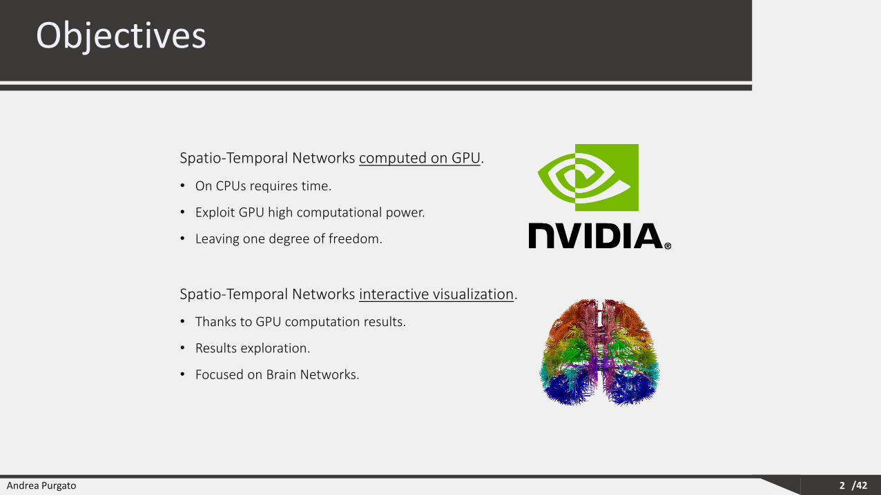
Spatio-Temporal Networks computed on GPU.
• On CPUs requires time.
• Exploit GPU high computational power.
• Leaving one degree of freedom.
Spatio-Temporal Networks interactive visualization.
• Thanks to GPU computation results.
• Results exploration.
• Focused on Brain Networks.
Andrea Purgato /42
Outline
3
1. Spatio-Temporal Network
2. GPU Programming Model
3. Similarity Computation
4. Experimental Evaluation
5. Brain Network Visualization
6. Final Considerations

Andrea Purgato /42
Outline
4
1. Spatio-Temporal Network
2. GPU Programming Model
3. Similarity Computation
4. Experimental Evaluation
5. Brain Network Visualization
6. Final Considerations
Andrea Purgato /42
Spatio-Temporal Network (1/5)
5
• Spatio-Temporal Network represents an evolution of usual graphs.
• Introduces the time component.
• Network structure changes during the time.
• Used to represent dynamic interactions among entities.
• Increased the graphs complexity.
• Applied to many different contexts. [1]
[1] Holme, P.: Modern temporal network theory: a colloquium.
Andrea Purgato /42
Spatio-Temporal Network (2/5)
6
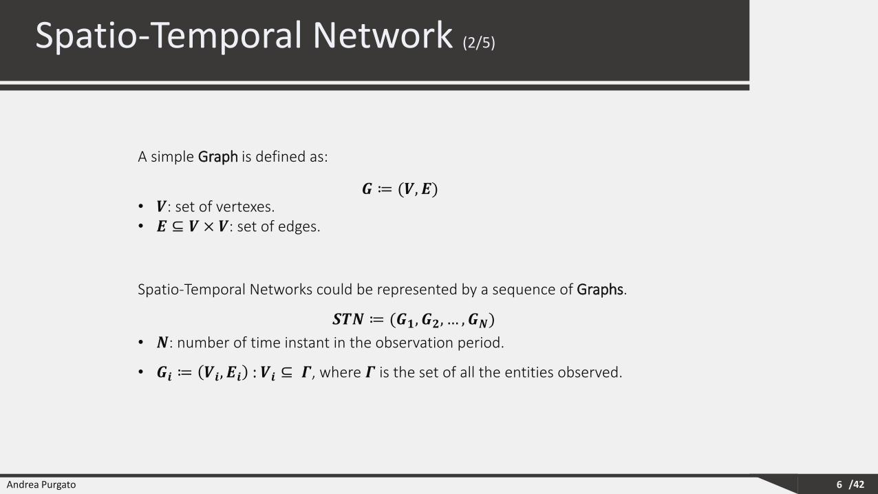
A simple Graph is defined as:
𝑮 ≔ (𝑽, 𝑬)• 𝑽: set of vertexes.• 𝑬 ⊆ 𝑽 × 𝑽: set of edges.
Spatio-Temporal Networks could be represented by a sequence of Graphs.
𝑺𝑻𝑵 ≔ (𝑮𝟏, 𝑮𝟐, … , 𝑮𝑵)
• 𝑵: number of time instant in the observation period.
• 𝑮𝒊 ≔ 𝑽𝒊, 𝑬𝒊 : 𝑽𝒊 ⊆ 𝜞, where 𝜞 is the set of all the entities observed.
Andrea Purgato /42
Spatio-Temporal Network (3/5)
7
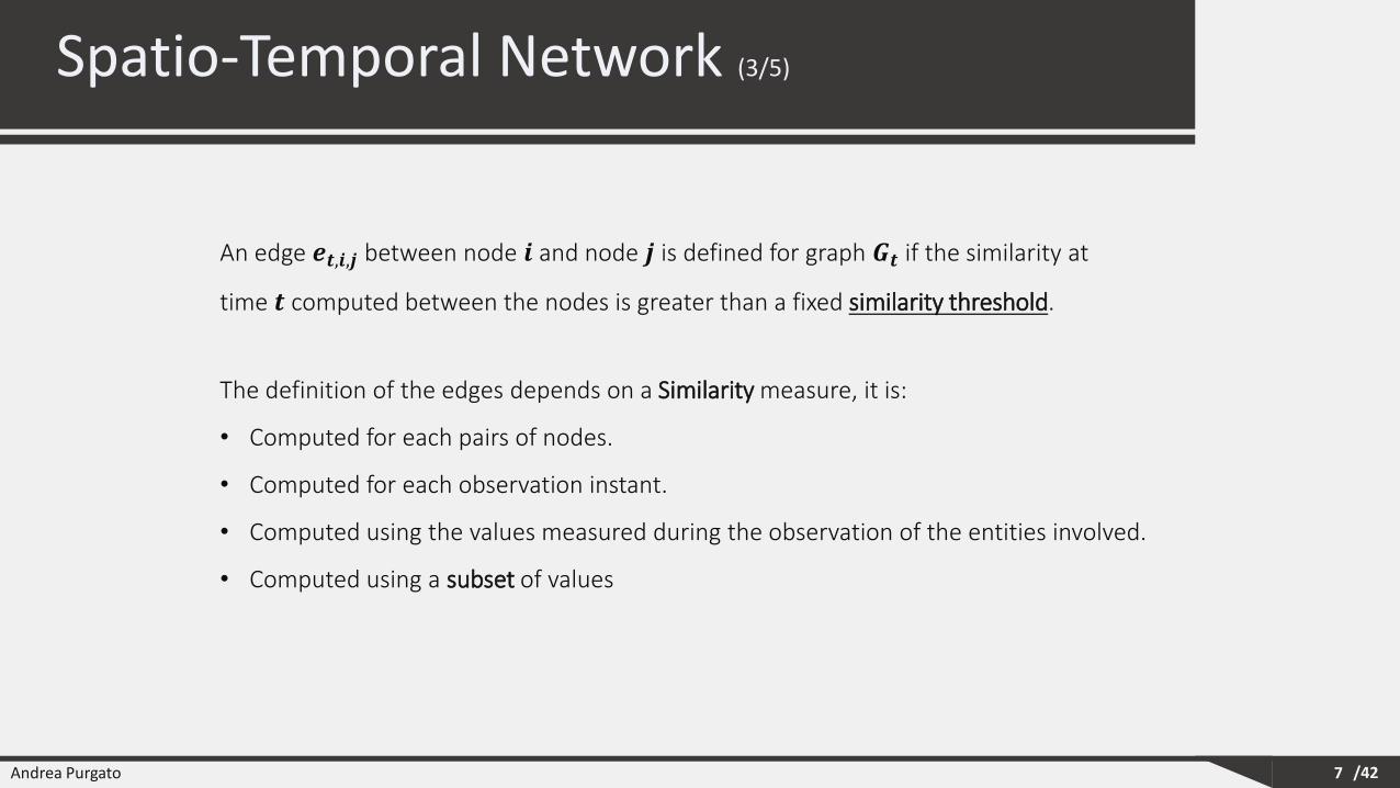
The definition of the edges depends on a Similarity measure, it is:
• Computed for each pairs of nodes.
• Computed for each observation instant.
• Computed using the values measured during the observation of the entities involved.
• Computed using a subset of values
An edge 𝒆𝒕,𝒊,𝒋 between node 𝒊 and node 𝒋 is defined for graph 𝑮𝒕 if the similarity at
time 𝒕 computed between the nodes is greater than a fixed similarity threshold.
Andrea Purgato /42
Spatio-Temporal Network (4/5)
8
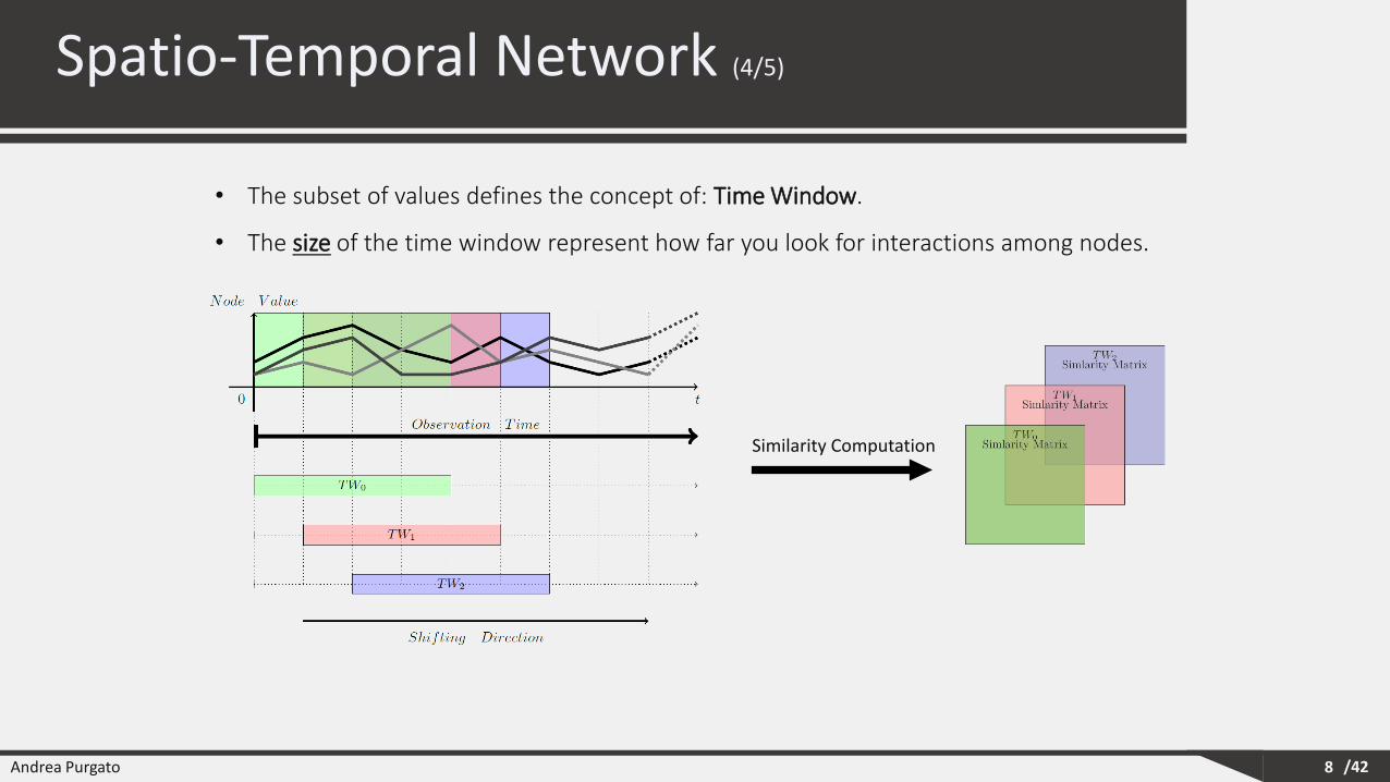
• The subset of values defines the concept of: Time Window.
• The size of the time window represent how far you look for interactions among nodes.
Similarity Computation
Andrea Purgato /42
Spatio-Temporal Network (5/5)
9
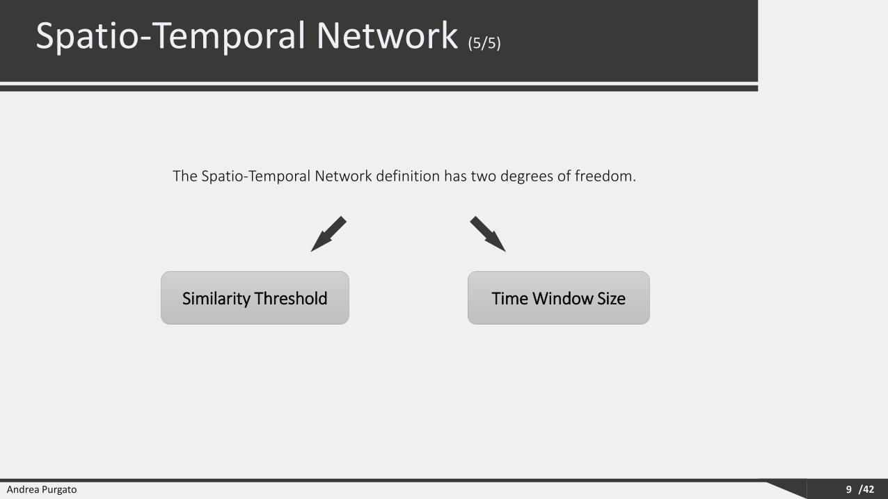
The Spatio-Temporal Network definition has two degrees of freedom.
Time Window SizeSimilarity Threshold

Andrea Purgato /42
Outline
10
1. Spatio-Temporal Network
2. GPU Programming Model
3. Similarity Computation
4. Experimental Evaluation
5. Brain Network Visualization
6. Final Considerations
Andrea Purgato /42
GPU Programming Model (1/4)
11
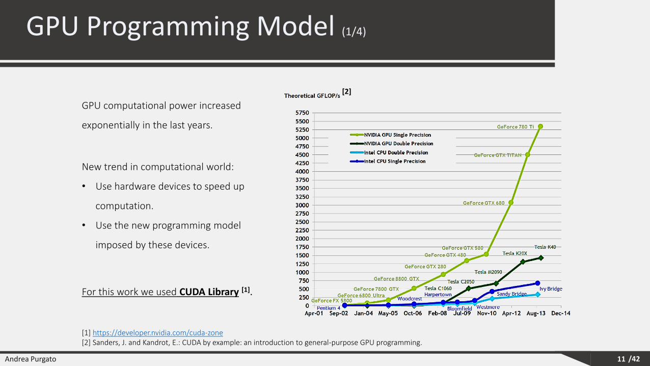
GPU computational power increased
exponentially in the last years.
New trend in computational world:
• Use hardware devices to speed up
computation.
• Use the new programming model
imposed by these devices.
For this work we used CUDA Library [1].
[1] https://developer.nvidia.com/cuda-zone[2] Sanders, J. and Kandrot, E.: CUDA by example: an introduction to general-purpose GPU programming.
[2]
Andrea Purgato /42
GPU Programming Model (2/4)
12
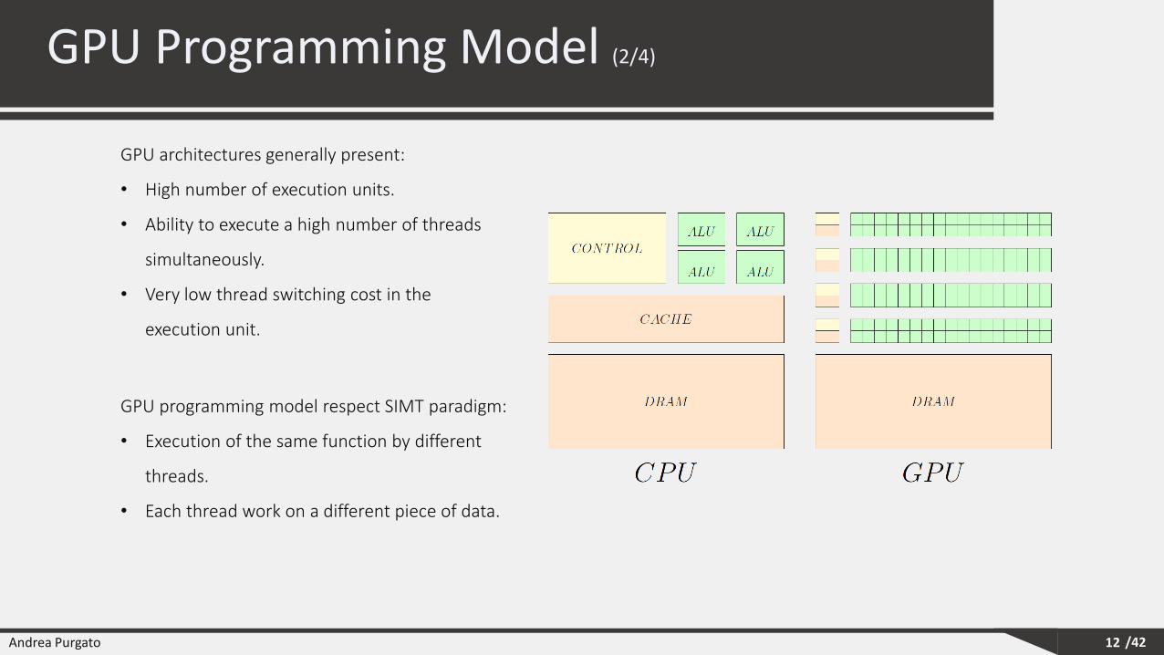
GPU architectures generally present:
• High number of execution units.
• Ability to execute a high number of threads
simultaneously.
• Very low thread switching cost in the
execution unit.
GPU programming model respect SIMT paradigm:
• Execution of the same function by different
threads.
• Each thread work on a different piece of data.
Andrea Purgato /42
GPU Programming Model (3/4)
13
Architectures that support CUDA programming presents two main components:
• Global Memory (GM)
• Streaming Multiprocessor (SM)
Function executed by a GPU thread called: Kernel Function.
• Executed after a GPU call performed by the CPU.
• Each call must have associated a GPU Structure.
Streaming Multiprocessor:
• Collection of execution units.
• Independent each other.
• Execute threads in bunch, called Warps.
Andrea Purgato /42
GPU Programming Model (4/4)
14
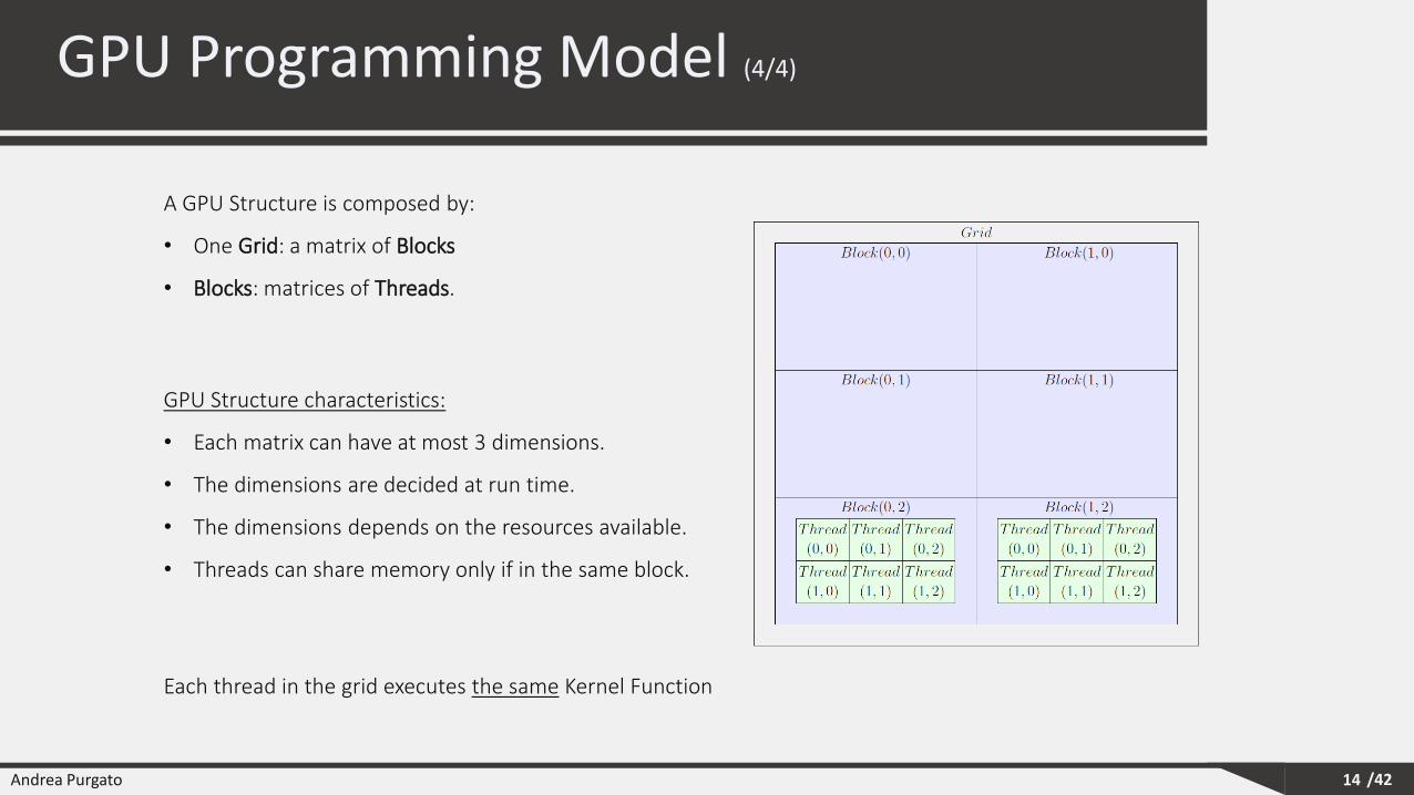
A GPU Structure is composed by:
• One Grid: a matrix of Blocks
• Blocks: matrices of Threads.
Each thread in the grid executes the same Kernel Function
GPU Structure characteristics:
• Each matrix can have at most 3 dimensions.
• The dimensions are decided at run time.
• The dimensions depends on the resources available.
• Threads can share memory only if in the same block.

Andrea Purgato /42
Outline
15
1. Spatio-Temporal Network
2. GPU Programming Model
3. Similarity Computation
4. Experimental Evaluation
5. Brain Network Visualization
6. Final Considerations
Andrea Purgato /42
Similarity Computation
16
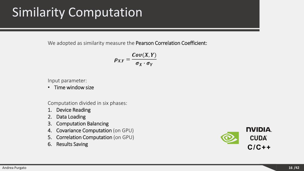
Computation divided in six phases:1. Device Reading2. Data Loading3. Computation Balancing4. Covariance Computation (on GPU)5. Correlation Computation (on GPU)6. Results Saving
We adopted as similarity measure the Pearson Correlation Coefficient:
𝝆𝑿,𝒀 =𝑪𝒐𝒗(𝑿, 𝒀)
𝝈𝑿 ∙ 𝝈𝒀
Input parameter:• Time window size
Andrea Purgato /42
1. Device Reading
17
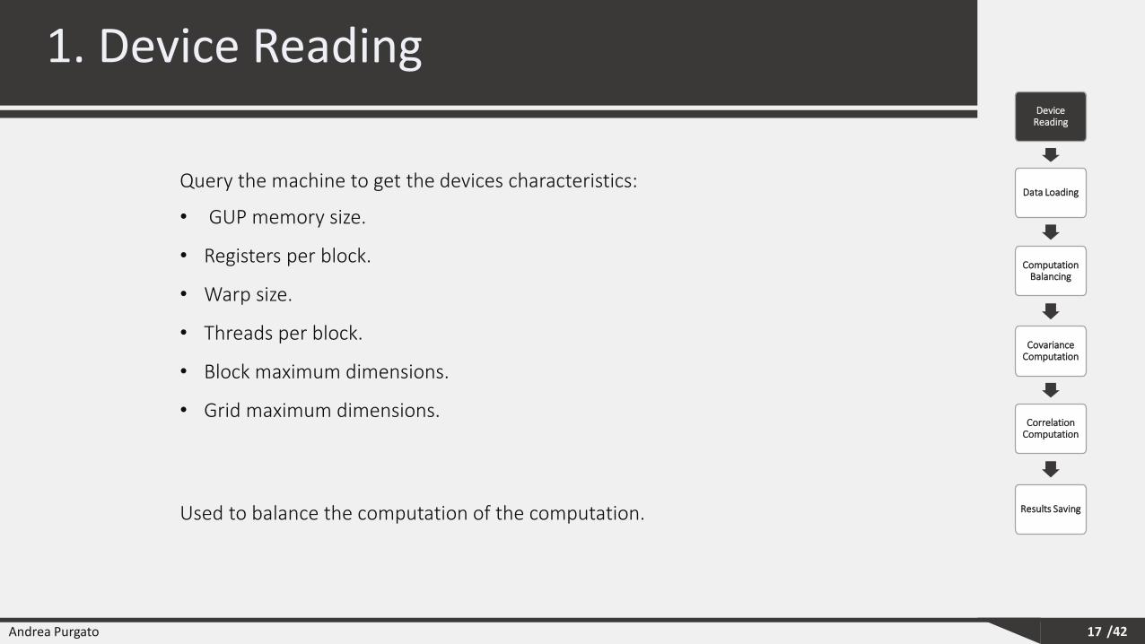
Query the machine to get the devices characteristics:
• GUP memory size.
• Registers per block.
• Warp size.
• Threads per block.
• Block maximum dimensions.
• Grid maximum dimensions.
Used to balance the computation of the computation.
Device Reading
Data Loading
Computation Balancing
Covariance Computation
Correlation Computation
Results Saving
Andrea Purgato /42
2. Data Loading
18
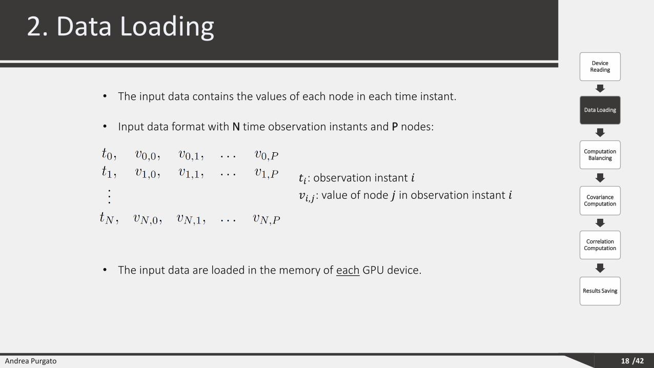
• Input data format with N time observation instants and P nodes:
𝑡𝑖: observation instant 𝑖
𝑣𝑖,𝑗: value of node 𝑗 in observation instant 𝑖
• The input data contains the values of each node in each time instant.
• The input data are loaded in the memory of each GPU device.
Device Reading
Data Loading
Computation Balancing
Covariance Computation
Correlation Computation
Results Saving
Andrea Purgato /42
3. Computation Balancing (1/4)
19
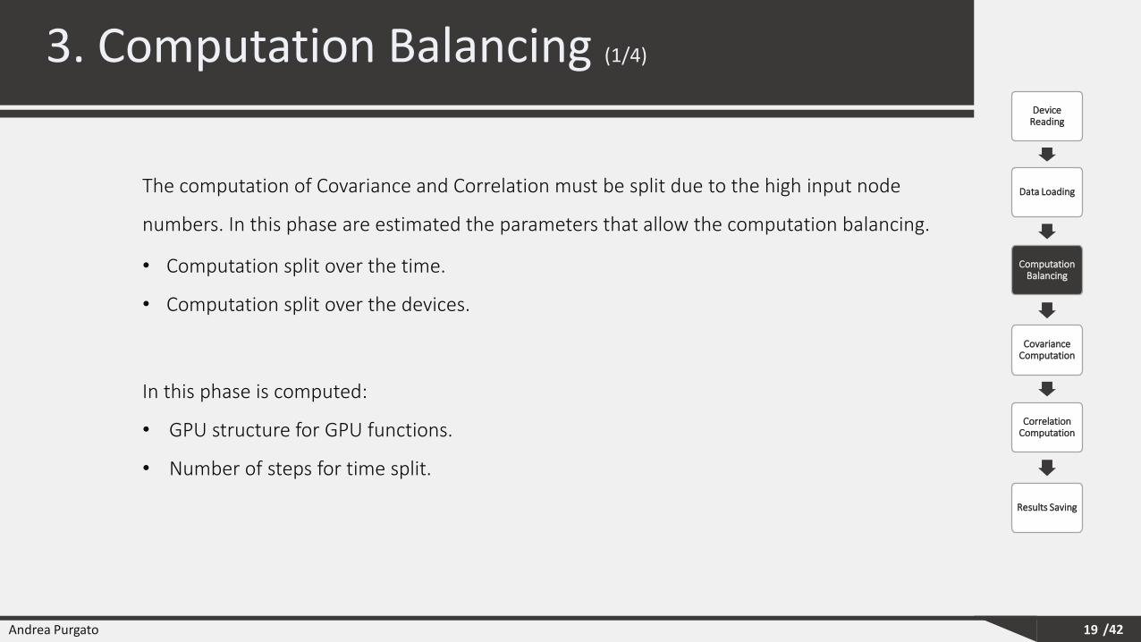
The computation of Covariance and Correlation must be split due to the high input node
numbers. In this phase are estimated the parameters that allow the computation balancing.
Device Reading
Data Loading
Computation Balancing
Covariance Computation
Correlation Computation
Results Saving
• Computation split over the time.
• Computation split over the devices.
In this phase is computed:
• GPU structure for GPU functions.
• Number of steps for time split.
Andrea Purgato /42
3. Computation Balancing (2/4)
20
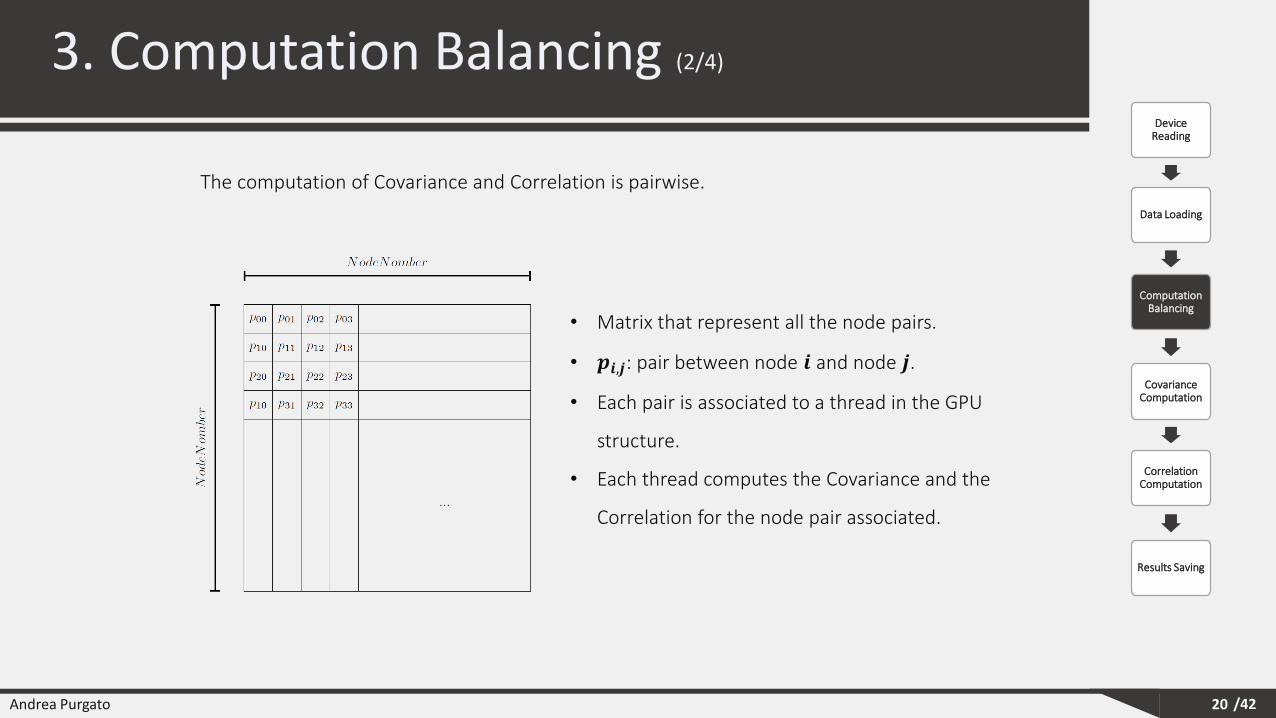
The computation of Covariance and Correlation is pairwise.
Device Reading
Data Loading
Computation Balancing
Covariance Computation
Correlation Computation
Results Saving
• Matrix that represent all the node pairs.
• 𝒑𝒊,𝒋: pair between node 𝒊 and node 𝒋.
• Each pair is associated to a thread in the GPU
structure.
• Each thread computes the Covariance and the
Correlation for the node pair associated.
Andrea Purgato /42
3. Computation Balancing (3/4)
21
Device Reading
Data Loading
Computation Balancing
Covariance Computation
Correlation Computation
Results Saving
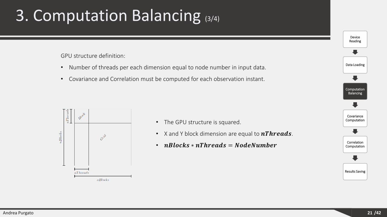
• The GPU structure is squared.
• X and Y block dimension are equal to 𝒏𝑻𝒉𝒓𝒆𝒂𝒅𝒔.
• 𝒏𝑩𝒍𝒐𝒄𝒌𝒔 ∗ 𝒏𝑻𝒉𝒓𝒆𝒂𝒅𝒔 = 𝑵𝒐𝒅𝒆𝑵𝒖𝒎𝒃𝒆𝒓
GPU structure definition:
• Number of threads per each dimension equal to node number in input data.
• Covariance and Correlation must be computed for each observation instant.
Andrea Purgato /42
3. Computation Balancing (3/4)
22
Device Reading
Data Loading
Computation Balancing
Covariance Computation
Correlation Computation
Results Saving
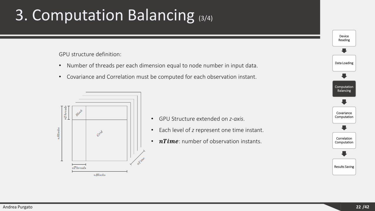
• GPU Structure extended on z-axis.
• Each level of z represent one time instant.
• 𝒏𝑻𝒊𝒎𝒆: number of observation instants.
GPU structure definition:
• Number of threads per each dimension equal to node number in input data.
• Covariance and Correlation must be computed for each observation instant.
Andrea Purgato /42
3. Computation Balancing (4/4)
23
Device Reading
Data Loading
Computation Balancing
Covariance Computation
Correlation Computation
Results Saving
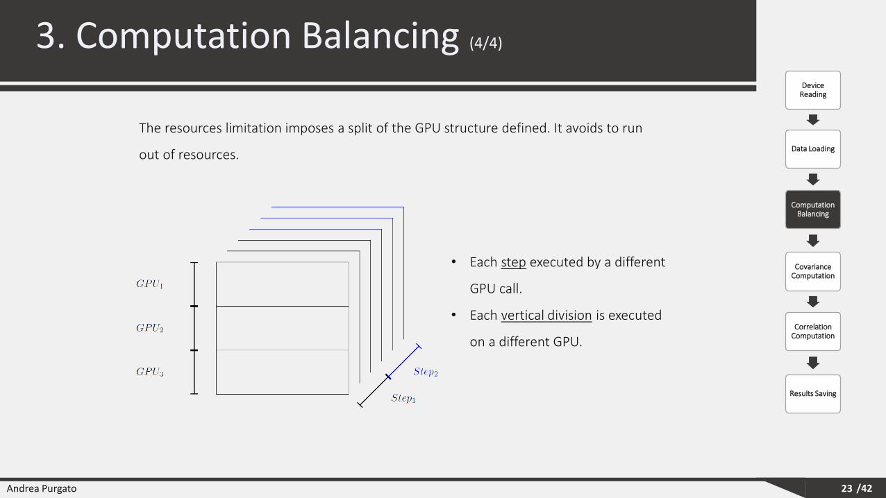
The resources limitation imposes a split of the GPU structure defined. It avoids to run
out of resources.
• Each step executed by a different
GPU call.
• Each vertical division is executed
on a different GPU.
Andrea Purgato /42
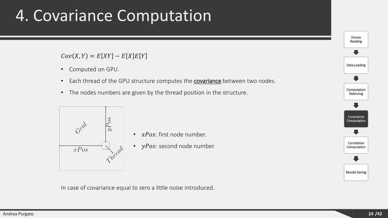
4. Covariance Computation
24
Device Reading
Data Loading
Computation Balancing
Covariance Computation
Correlation Computation
Results Saving
• 𝑥𝑃𝑜𝑠: first node number.
• 𝑦𝑃𝑜𝑠: second node number.
In case of covariance equal to zero a little noise introduced.
𝐶𝑜𝑣 𝑋, 𝑌 = 𝐸 𝑋𝑌 − 𝐸 𝑋 𝐸 𝑌
• Computed on GPU.
• Each thread of the GPU structure computes the covariance between two nodes.
• The nodes numbers are given by the thread position in the structure.
Andrea Purgato /42
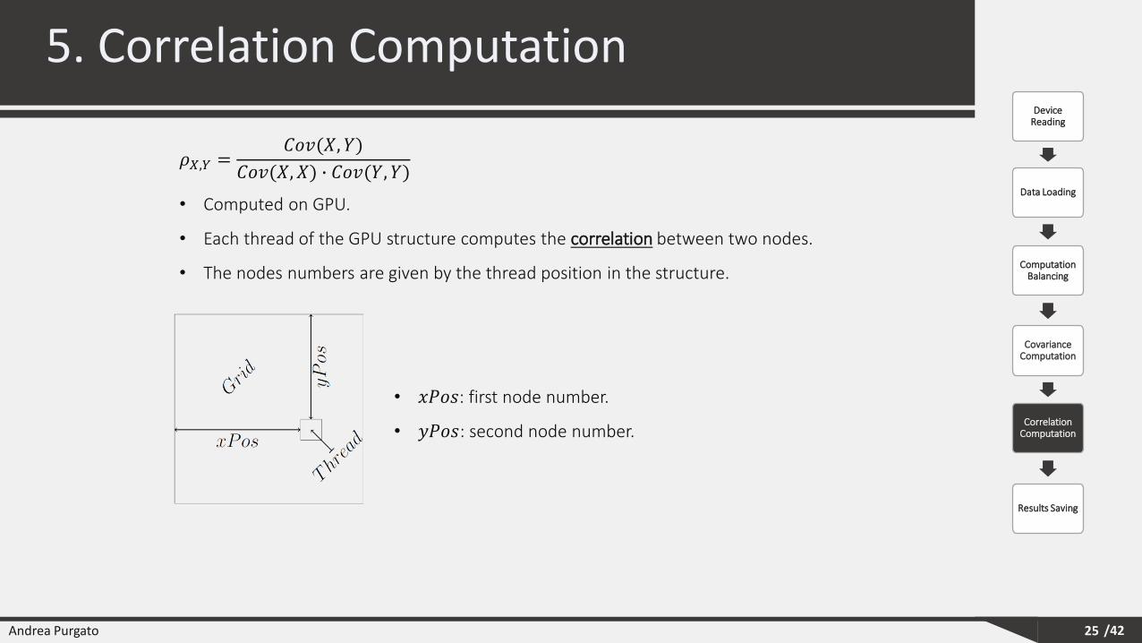
5. Correlation Computation
25
Device Reading
Data Loading
Computation Balancing
Covariance Computation
Correlation Computation
Results Saving
• 𝑥𝑃𝑜𝑠: first node number.
• 𝑦𝑃𝑜𝑠: second node number.
𝜌𝑋,𝑌 =𝐶𝑜𝑣(𝑋, 𝑌)
𝐶𝑜𝑣(𝑋, 𝑋) ∙ 𝐶𝑜𝑣(𝑌, 𝑌)
• Computed on GPU.
• Each thread of the GPU structure computes the correlation between two nodes.
• The nodes numbers are given by the thread position in the structure.
Andrea Purgato /42
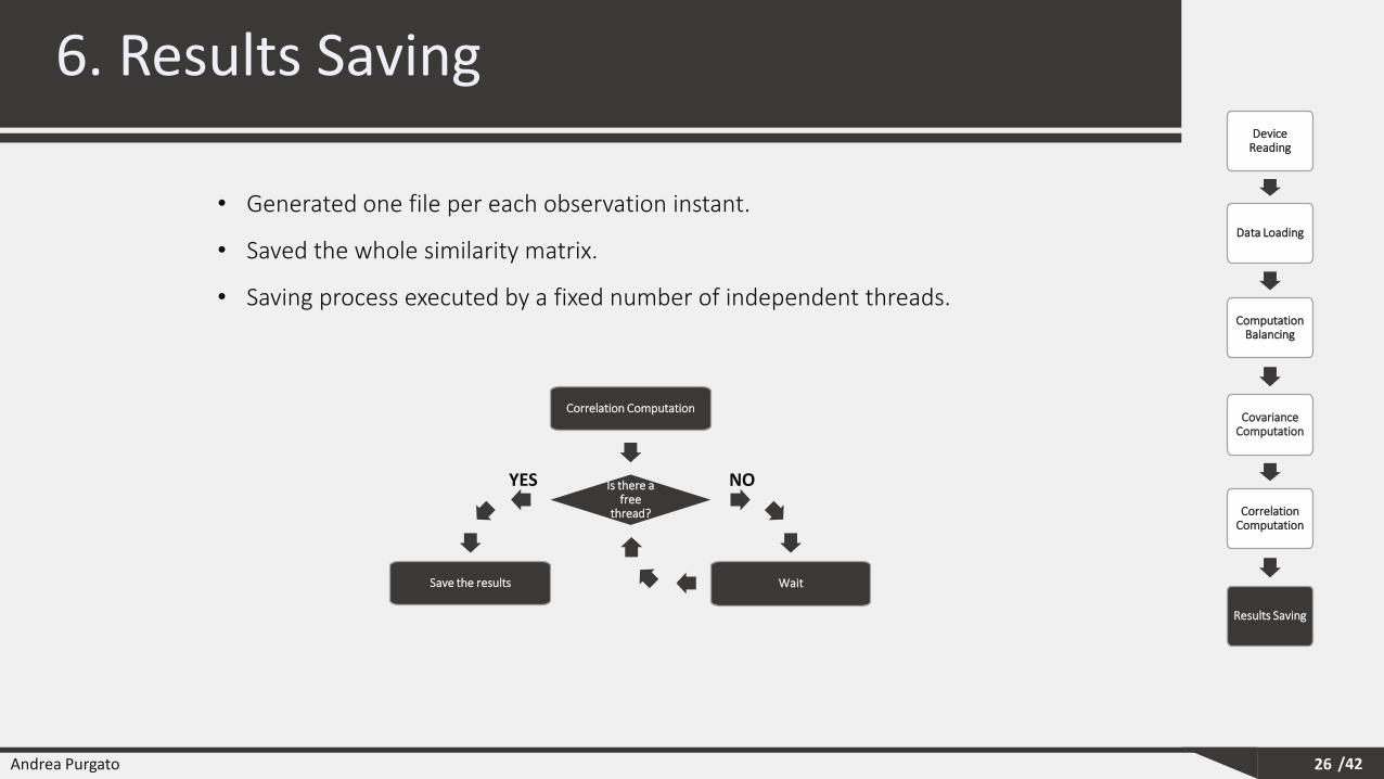
6. Results Saving
26
Device Reading
Data Loading
Computation Balancing
Covariance Computation
Correlation Computation
Results Saving
• Generated one file per each observation instant.
• Saved the whole similarity matrix.
• Saving process executed by a fixed number of independent threads.
Correlation Computation
Is there a free
thread?
Save the results Wait
YES NO

Andrea Purgato /42
Outline
27
1. Spatio-Temporal Network
2. GPU Programming Model
3. Similarity Computation
4. Experimental Evaluation
5. Brain Network Visualization
6. Final Considerations
Andrea Purgato /42
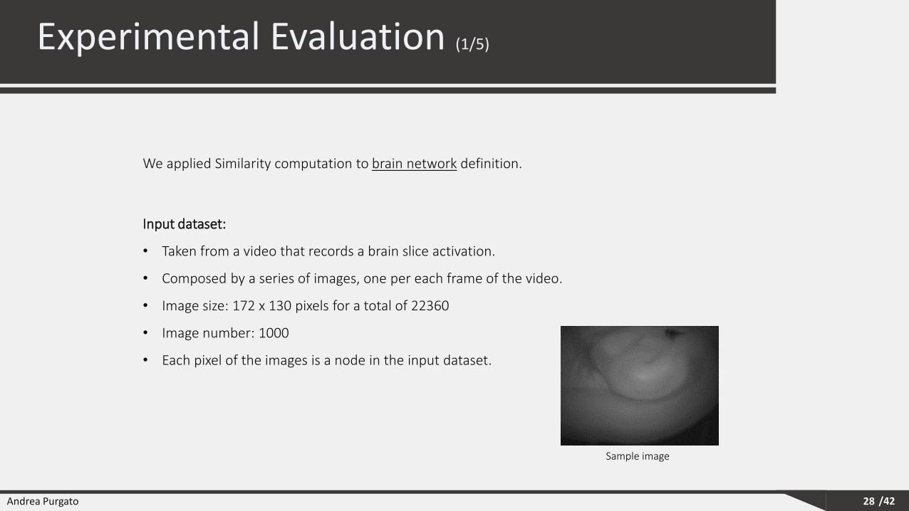
Experimental Evaluation (1/5)
28
Input dataset:
• Taken from a video that records a brain slice activation.
• Composed by a series of images, one per each frame of the video.
• Image size: 172 x 130 pixels for a total of 22360
• Image number: 1000
• Each pixel of the images is a node in the input dataset.
We applied Similarity computation to brain network definition.
Sample image

Andrea Purgato /42
Experimental Evaluation (2/5)
29
Each pixel is represented by a discrete function:
• For each observation instant is taken the pixel hue value.
• The discrete functions are transformed in the input file.
Andrea Purgato /42
Experimental Evaluation (3/5)
30
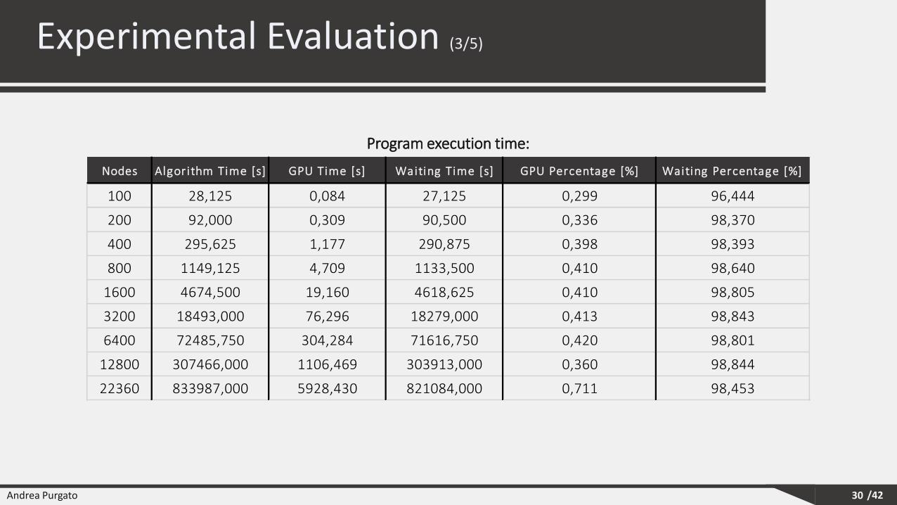
Program execution time:
Nodes Algorithm Time [s] GPU Time [s] Waiting Time [s] GPU Percentage [%] Waiting Percentage [%]
100 28,125 0,084 27,125 0,299 96,444
200 92,000 0,309 90,500 0,336 98,370
400 295,625 1,177 290,875 0,398 98,393
800 1149,125 4,709 1133,500 0,410 98,640
1600 4674,500 19,160 4618,625 0,410 98,805
3200 18493,000 76,296 18279,000 0,413 98,843
6400 72485,750 304,284 71616,750 0,420 98,801
12800 307466,000 1106,469 303913,000 0,360 98,844
22360 833987,000 5928,430 821084,000 0,711 98,453
Andrea Purgato /42
Experimental Evaluation (4/5)
31
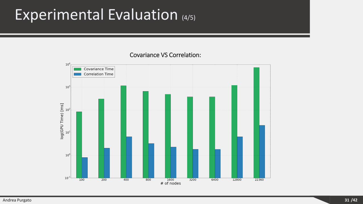
Covariance VS Correlation:
Andrea Purgato /42
Experimental Evaluation (5/5)
32
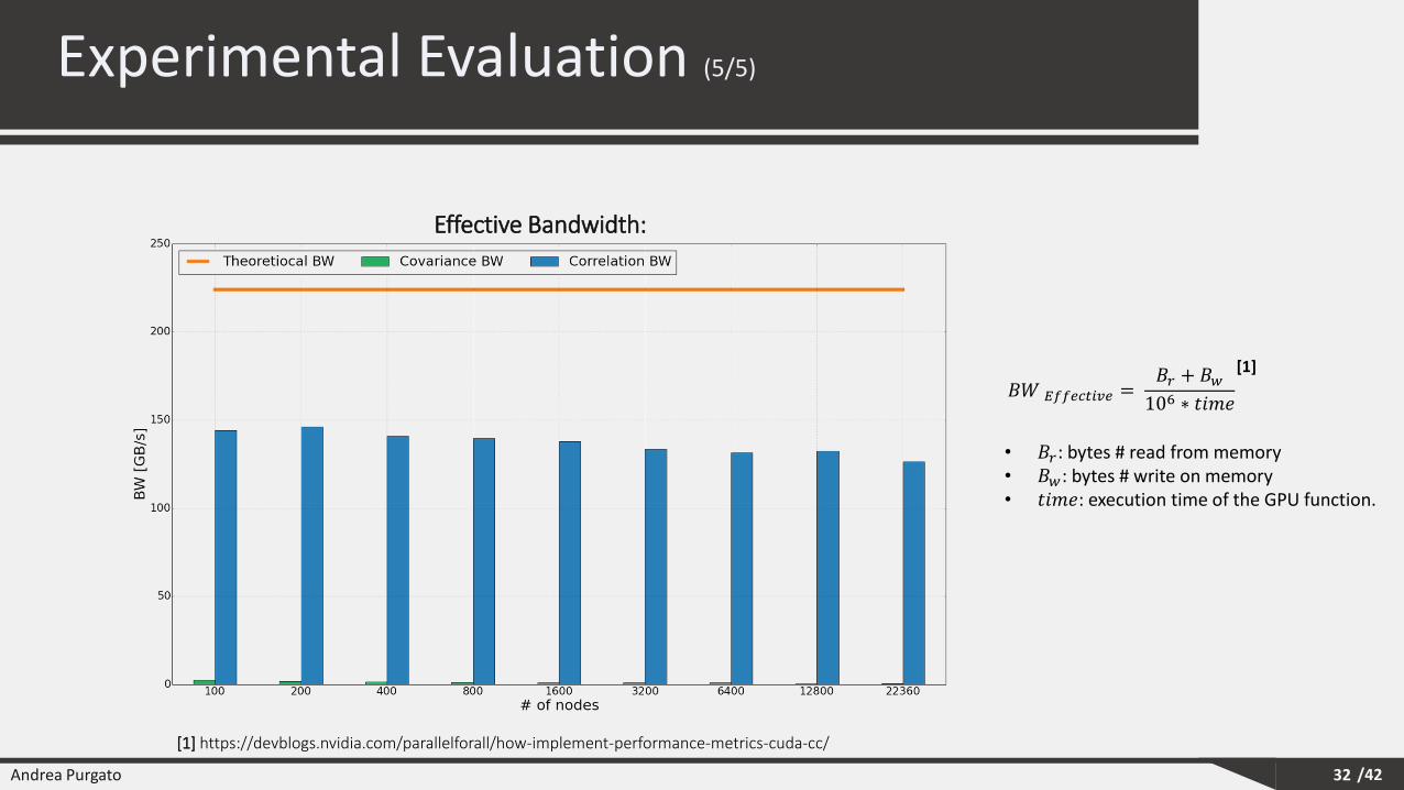
Effective Bandwidth:
𝐵𝑊 𝐸𝑓𝑓𝑒𝑐𝑡𝑖𝑣𝑒 =𝐵𝑟 + 𝐵𝑤106 ∗ 𝑡𝑖𝑚𝑒
• 𝐵𝑟: bytes # read from memory• 𝐵𝑤: bytes # write on memory• 𝑡𝑖𝑚𝑒: execution time of the GPU function.
[1]
[1] https://devblogs.nvidia.com/parallelforall/how-implement-performance-metrics-cuda-cc/

Andrea Purgato /42
Outline
33
1. Spatio-Temporal Network
2. GPU Programming Model
3. Similarity Computation
4. Experimental Evaluation
5. Brain Network Visualization
6. Final Considerations
Andrea Purgato /42
Brain Network Visualization (1/6)
34
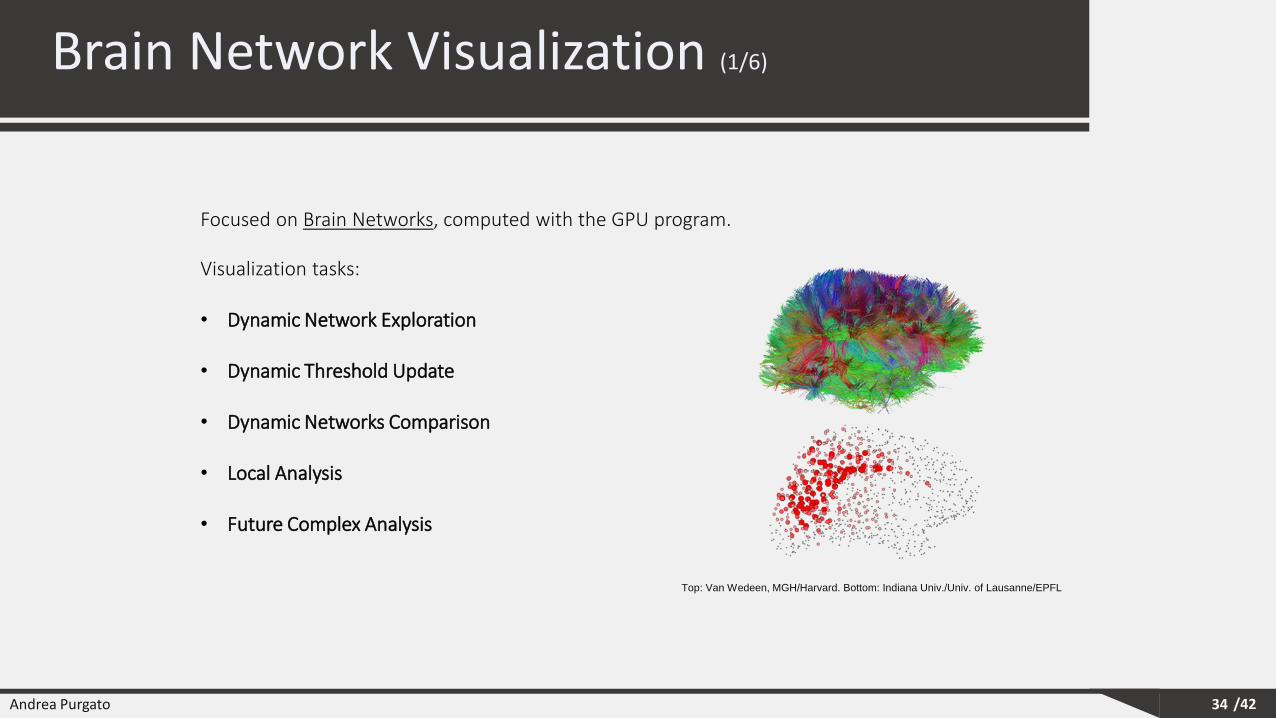
Focused on Brain Networks, computed with the GPU program.
Visualization tasks:
• Dynamic Network Exploration
• Dynamic Threshold Update
• Dynamic Networks Comparison
• Local Analysis
• Future Complex Analysis
Top: Van Wedeen, MGH/Harvard. Bottom: Indiana Univ./Univ. of Lausanne/EPFL
Andrea Purgato /42
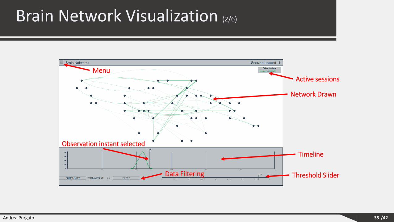
Brain Network Visualization (2/6)
35
Active sessions
Network Drawn
Timeline
Threshold Slider
Menu
Observation instant selected
Data Filtering
Andrea Purgato /42
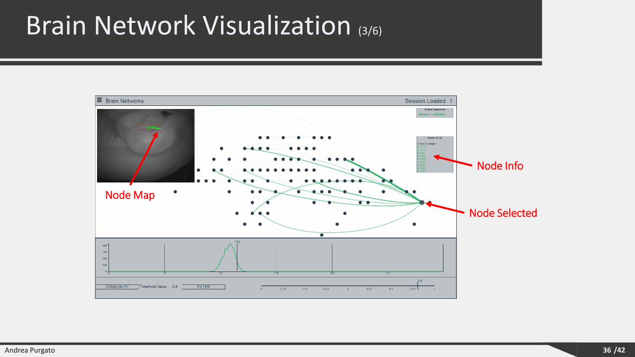
Brain Network Visualization (3/6)
36
Node Selected
Node Info
Node Map
Andrea Purgato /42
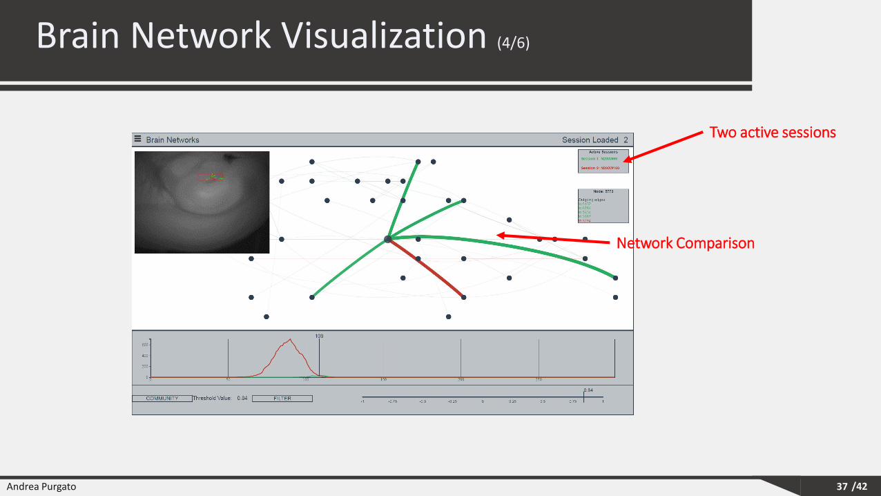
Brain Network Visualization (4/6)
37
Two active sessions
Network Comparison
Andrea Purgato /42
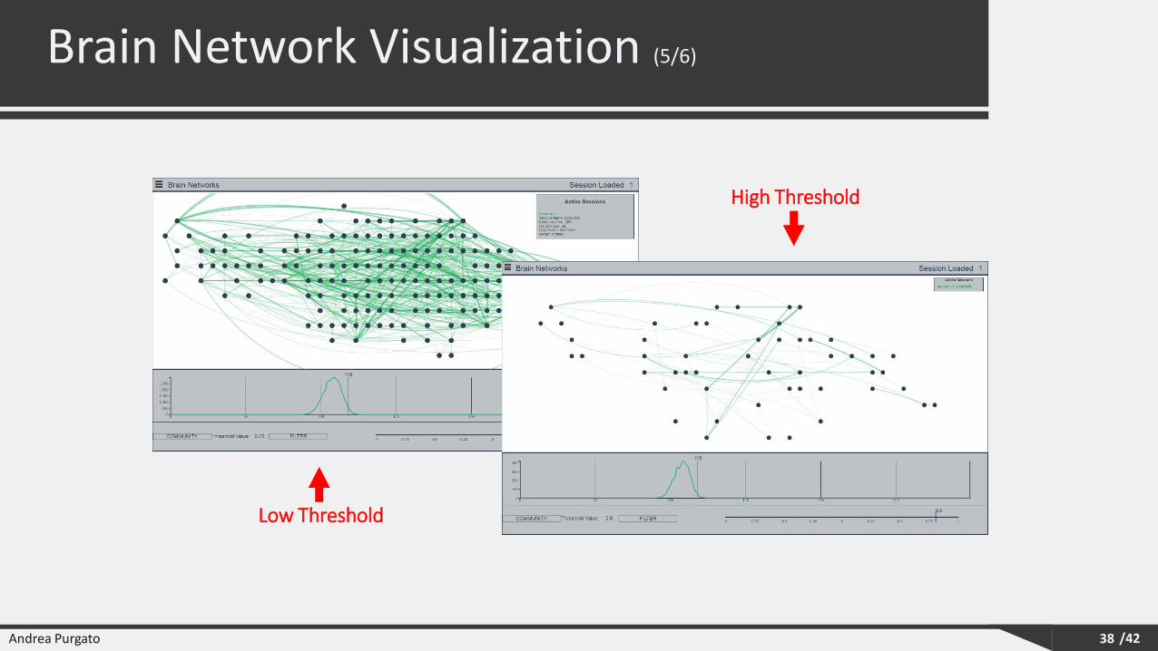
Brain Network Visualization (5/6)
38
Low Threshold
High Threshold
Andrea Purgato /42
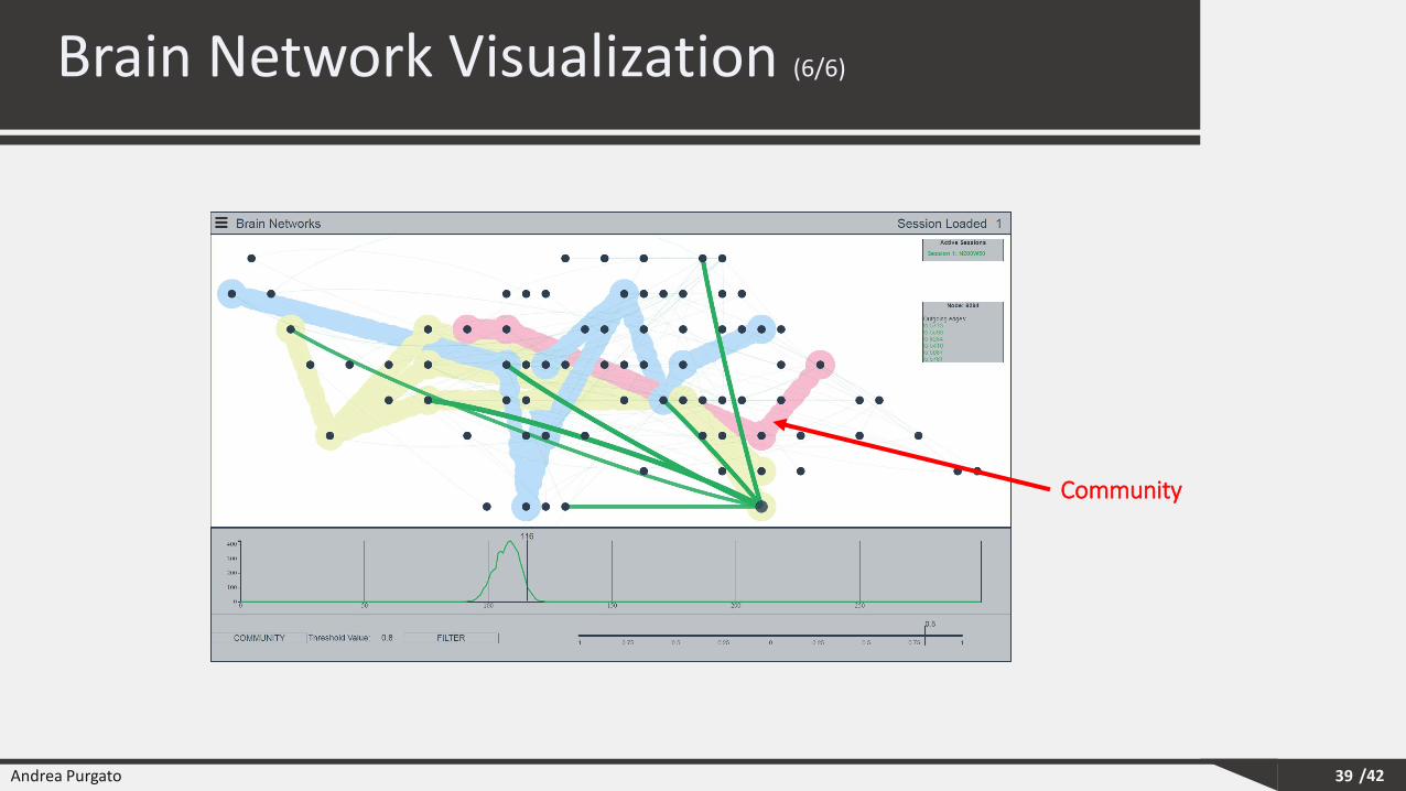
Brain Network Visualization (6/6)
39
Community
Andrea Purgato /42
Outline
40
1. Spatio-Temporal Network
2. GPU Programming Model
3. Similarity Computation
4. Experimental Evaluation
5. Brain Network Visualization
6. Final Considerations
Andrea Purgato /42
Final Considerations
41
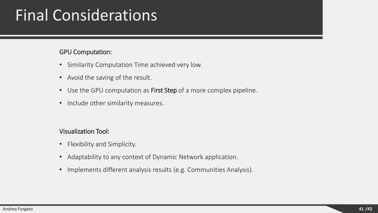
GPU Computation:
• Similarity Computation Time achieved very low.
• Avoid the saving of the result.
• Use the GPU computation as First Step of a more complex pipeline.
• Include other similarity measures.
Visualization Tool:
• Flexibility and Simplicity.
• Adaptability to any context of Dynamic Network application.
• Implements different analysis results (e.g. Communities Analysis).

/42Andrea Purgato 42
QUESTIONS?
Thanks for your attention!


