Gradient-based Methods for Optimization. Part II. Prof. Nathan L. Gibson Department of Mathematics Applied Math and Computation Seminar October 28, 2011 Prof. Gibson (OSU) Gradient-based Methods for Optimization AMC 2011 1 / 42
Transcript
Gradient-based Methods for Optimization. Part II.
Prof. Nathan L. Gibson
Department of Mathematics
Applied Math and Computation SeminarOctober 28, 2011
Prof. Gibson (OSU) Gradient-based Methods for Optimization AMC 2011 1 / 42
Summary from Last Time
Summary from Last Time
Unconstrained OptimizationNonlinear Least Squares
Parameter ID Problem
Sample Problem:
u′′ + cu′ + ku = 0; u(0) = u0; u′(0) = 0 (1)
Assume data {uj}Mj=0 is given for some times tj on the interval [0,T ]. Find
x=[c , k]T such that the following objective function is minimized:
f (x) =1
2
M∑j=1
|u(tj ; x)− uj |2 .
Prof. Gibson (OSU) Gradient-based Methods for Optimization AMC 2011 2 / 42
Summary from Last Time
Summary Continued
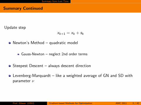
Update stepxk+1 = xk + sk
Newton’s Method – quadratic model
Gauss-Newton – neglect 2nd order terms
Steepest Descent – always descent direction
Levenberg-Marquardt – like a weighted average of GN and SD withparameter ν
Prof. Gibson (OSU) Gradient-based Methods for Optimization AMC 2011 3 / 42
Summary from Last Time
Summary of Methods
Newton:
mNk (x) = f (xk) +∇f (xk)
T (x − xk) +1
2(x − xk)
T∇2f (xk)(x − xk)
Gauss-Newton:
mGNk (x) = f (xk) +∇f (xk)
T (x − xk) +1
2(x − xk)
TR ′(xk)TR ′(xk)(x − xk)
Steepest Descent:
mSDk (x) = f (xk) +∇f (xk)
T (x − xk) +1
2(x − xk)
T 1
λkI (x − xk)
Levenberg-Marquardt:
mLMk (x) = f (xk)+∇f (xk)
T (x−xk)+1
2(x−xk)
T(R ′(xk)
TR ′(xk) + νk I)(x−xk)
0 = ∇mk(x) =⇒ Hksk = −∇f (xk)
Prof. Gibson (OSU) Gradient-based Methods for Optimization AMC 2011 4 / 42
Summary from Last Time
Levenberg-Marquardt Idea
If iterate is not close enough to minimizer so that GN does not give adescent direction, increase ν to take more of a SD direction.
As you get closer to minimizer, decrease ν to take more of a GN step.
For zero-residual problems, GN converges quadratically (if at all)SD converges linearly (guaranteed)
Prof. Gibson (OSU) Gradient-based Methods for Optimization AMC 2011 5 / 42
Summary from Last Time
LM Alternative Perspective
Approximate Hessian may not be positive definite (orwell-conditioned), increase ν to add regularity.
As you get closer to minimizer, Hessian will become positive definite.Decrease ν as less regularization is necessary.
Regularized problem is “nearby problem”, want to solve actualproblem as soon as feasible.
Prof. Gibson (OSU) Gradient-based Methods for Optimization AMC 2011 6 / 42
Outline
Line Search (Armijo Rule)
Damped Gauss-NewtonLMA
Levenberg-Marquardt Parameter
Polynomial Models
Trust Region
Changing TR RadiusChanging LM Parameter
Prof. Gibson (OSU) Gradient-based Methods for Optimization AMC 2011 7 / 42
Line Search
Step Length
Steepest Descent Method
We define the steepest descent direction to be dk = −∇f (xk). Thisdefines a direction but not a step length.
We define the Steepest Descent update step to be sSDk = λkdk for
some λk > 0.
We would like to choose λk so that f (x) decreases sufficiently.
If we ask simply thatf (xk+1) < f (xk)
Steepest Descent might not converge.
Prof. Gibson (OSU) Gradient-based Methods for Optimization AMC 2011 8 / 42
Line Search Sufficient Decrease
Predicted Reduction
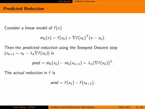
Consider a linear model of f (x)
mk(x) = f (xk) +∇f (xk)T (x − xk).
Then the predicted reduction using the Steepest Descent step(xk+1 = xk − λk∇f (xk)) is
pred = mk(xk)−mk(xk+1) = λk‖∇f (xk)‖2.
The actual reduction in f is
ared = f (xk)− f (xk+1).
Prof. Gibson (OSU) Gradient-based Methods for Optimization AMC 2011 9 / 42
Line Search Sufficient Decrease
Sufficient Decrease
We define a sufficient decrease to be when
ared ≥ α pred ,
where α ∈ (0, 1) (e.g., 10−4 or so).Note: α = 0 is simple decrease.
Prof. Gibson (OSU) Gradient-based Methods for Optimization AMC 2011 10 / 42
Line Search Armijo Rule
Armijo Rule
We can define a strategy for determining the step length in terms of asufficient decrease criteria as follows:Let λ = βm, where β ∈ (0, 1) (think 1
2) and m ≥ 0 is the smallest integersuch that
ared > α pred ,
where α ∈ (0, 1).
Prof. Gibson (OSU) Gradient-based Methods for Optimization AMC 2011 11 / 42
Line Search Armijo Rule
Line Search
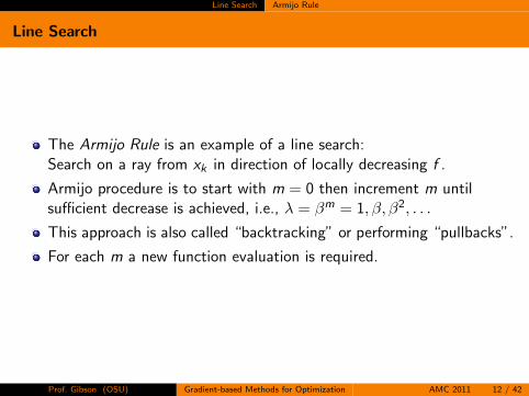
The Armijo Rule is an example of a line search:Search on a ray from xk in direction of locally decreasing f .
Armijo procedure is to start with m = 0 then increment m untilsufficient decrease is achieved, i.e., λ = βm = 1, β, β2, . . .
This approach is also called “backtracking” or performing “pullbacks”.
For each m a new function evaluation is required.
Prof. Gibson (OSU) Gradient-based Methods for Optimization AMC 2011 12 / 42
Line Search Damped Gauss-Newton
Damped Gauss-Newton
Armijo Rule applied to the Gauss-Newton step is called the DampedGauss-Newton Method.
Recall
dGN = −(R ′(x)TR ′(x)
)−1R ′(x)TR(x).
Note that if R ′(x) has full column rank, then
0 > ∇f (x)TdGN =
−(R ′(x)TR(x)
)T (R ′(x)TR ′(x)
)−1R ′(x)TR(x)
so the GN direction is a descent direction.
Prof. Gibson (OSU) Gradient-based Methods for Optimization AMC 2011 13 / 42
Line Search Damped Gauss-Newton
Damped Gauss-Newton Step
Thus the step for Damped Gauss-Newton is
sDGN = βmdGN
where β ∈ (0, 1) and m is the smallest non-negative integer to guaranteesufficient decrease.
Prof. Gibson (OSU) Gradient-based Methods for Optimization AMC 2011 14 / 42
Line Search LMA
Levenberg-Marquardt-Armijo
If R ′(x) does not have full column rank, or if the matrix R ′(x)TR ′(x)may be ill-conditioned, you should be using Levenberg-Marquardt.
The LM direction is a descent direction.
Line search can be applied.
Can show that if νk = O(‖R(xk)‖) then LMA converges quadraticallyfor (nice) zero residual problems.
Prof. Gibson (OSU) Gradient-based Methods for Optimization AMC 2011 15 / 42
Line Search
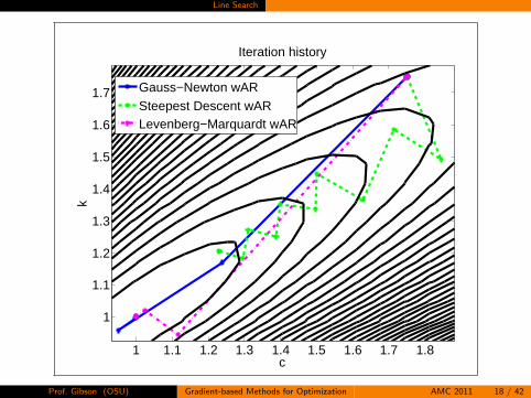
Numerical Example
Recallu′′ + cu′ + ku = 0; u(0) = u0; u
′(0) = 0.
Let the true parameters be x∗ = [c , k]T = [1, 1]T . Assume we haveM = 100 data uj from equally spaced time points on [0, 10].
We will use the initial iterate x0 = [3, 1]T with Steepest Descent,Gauss-Newton and Levenberg-Marquardt methods using the ArmijoRule.
Prof. Gibson (OSU) Gradient-based Methods for Optimization AMC 2011 16 / 42
Line Search
0.8 1 1.2 1.4 1.6 1.8 2
0.6
0.8
1
1.2
1.4
1.6
1.8
c
k
Search Direction
Gauss−NewtonSteepest DescentLevenberg−Marquardt
Prof. Gibson (OSU) Gradient-based Methods for Optimization AMC 2011 17 / 42
Line Search
1 1.1 1.2 1.3 1.4 1.5 1.6 1.7 1.8
1
1.1
1.2
1.3
1.4
1.5
1.6
1.7
c
k
Iteration history
Gauss−Newton wARSteepest Descent wARLevenberg−Marquardt wAR
Prof. Gibson (OSU) Gradient-based Methods for Optimization AMC 2011 18 / 42
Line Search
0 1 2 3 4 510
−8
10−6
10−4
10−2
100
102
Iterations
Gra
dien
t Nor
m
Gauss−Newton with Armijo rule
0 1 2 3 4 510
−15
10−10
10−5
100
105
Iterations
Fun
ctio
n V
alue
Gauss−Newton with Armijo rule
0 2 4 6 8 10
101.4
101.5
101.6
101.7
Iterations
Gra
dien
t Nor
m
Steepest Descent with Armijo rule
0 2 4 6 8 1010
0
101
102
103
104
Iterations
Fun
ctio
n V
alue
Steepest Descent with Armijo rule
Prof. Gibson (OSU) Gradient-based Methods for Optimization AMC 2011 19 / 42
Line Search
0 1 2 3 4 510
−8
10−6
10−4
10−2
100
102
Iterations
Gra
dien
t Nor
m
Gauss−Newton with Armijo rule
0 1 2 3 4 510
−15
10−10
10−5
100
105
Iterations
Fun
ctio
n V
alue
Gauss−Newton with Armijo rule
IterationsPullbacks
0 2 4 6 8 10
101.4
101.5
101.6
101.7
Iterations
Gra
dien
t Nor
m
Steepest Descent with Armijo rule
0 2 4 6 8 1010
0
101
102
103
104
Iterations
Fun
ctio
n V
alue
Steepest Descent with Armijo rule
IterationsPullbacks
Prof. Gibson (OSU) Gradient-based Methods for Optimization AMC 2011 20 / 42
Levenberg-Marquardt Parameter
Word of Caution for LM
Note that blindly increasing ν until a sufficient decrease criteria issatisfied is NOT a good idea (nor is it a line search).
Changing ν changes direction as well as step length.
Increasing ν does insure your direction is descending.
But, increasing ν too much makes your step length small.
Prof. Gibson (OSU) Gradient-based Methods for Optimization AMC 2011 21 / 42
Levenberg-Marquardt Parameter
1 1.5 2 2.5 3 3.5 4 4.51
1.2
1.4
1.6
1.8
2
2.2
2.4
c
k
Levenberg−Marquardt step
ν=1ν=2ν=4
Prof. Gibson (OSU) Gradient-based Methods for Optimization AMC 2011 22 / 42
Levenberg-Marquardt Parameter
1 1.5 2 2.5 31
1.1
1.2
1.3
1.4
1.5
1.6
1.7
c
k
Levenberg−Marquardt step
ν=100ν=200ν=400
Prof. Gibson (OSU) Gradient-based Methods for Optimization AMC 2011 23 / 42
Polynomial Models
Line Search Improvements
Step length control with polynomial models
If λ = 1 does not give sufficient decrease, use f (xk), f (xk + d) and∇f (xk) to build a quadratic model of
ξ(λ) = f (xk + λd)
Compute the λ which minimizes model of ξ.
If this fails, create cubic model.
If this fails, switch back to Armijo.
Exact line search is (usually) not worth the cost.
Prof. Gibson (OSU) Gradient-based Methods for Optimization AMC 2011 24 / 42
Trust Region Methods
Trust Region Methods
Let ∆ be the radius of a ball about xk inside which the quadraticmodel
mk(x) = f (xk) +∇f (xk)T (x − xk)
+1
2(x − xk)THk(x − xk)
can be “trusted” to accurately represent f (x).
∆ is called the trust region radius.
T (∆) = {x | ‖x − xk‖ ≤ ∆} is called the trust region.
Prof. Gibson (OSU) Gradient-based Methods for Optimization AMC 2011 25 / 42
Trust Region Methods
Trust Region Problem
We compute a trial solution xt , which may or may not become ournext iterate.
We define the trial solution in terms of a trial step xt = xk + st .
The trial step is the (approximate) solution to the trust regionproblem
min‖s‖≤∆
mk(xk + s).
I.e., find the trial solution in the trust region which minimizes thequadratic model of f .
Prof. Gibson (OSU) Gradient-based Methods for Optimization AMC 2011 26 / 42
Trust Region Methods Changing Trust Region Radius
Changing Trust Region Radius
Test the trial solution xt using predicted and actual reductions.
If µ = ared/pred too low, reject trial step and decrease trust regionradius.
If µ sufficiently high, we can accept the trial step, and possibly evenincrease the trust region radius (becoming more aggressive).
Prof. Gibson (OSU) Gradient-based Methods for Optimization AMC 2011 27 / 42
Trust Region Methods
Exact Solution to TR Problem
Theorem
Let g ∈ RN and let A be a symmetric N × N matrix. Let
m(s) = gT s + sTAs/2.
Then a vector s is a solution to
min‖s‖≤∆
m(s)
if and only if there is some ν ≥ 0 such that
(A + νI )s = −g
and either ν = 0 or ‖s‖ = ∆.
Prof. Gibson (OSU) Gradient-based Methods for Optimization AMC 2011 28 / 42
Trust Region Methods LM as a TRM
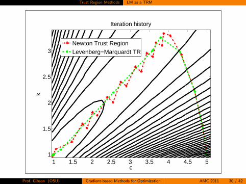
LM as a TRM
Instead of controlling ∆ in response to µ = ared/pred , adjust ν.
Start with ν = ν0 and compute xt = xk + sLM .
If µ = ared/pred too small, reject trial and increase ν. Recomputetrial (only requires a linear solve).
If µ sufficiently high, accept trial and possibly decrease ν (maybe to0).
Once trial accepted as an iterate, compute R, f , R ′, ∇f and test‖∇f ‖ for termination.
Prof. Gibson (OSU) Gradient-based Methods for Optimization AMC 2011 29 / 42
Trust Region Methods LM as a TRM
1 1.5 2 2.5 3 3.5 4 4.5 51
1.5
2
2.5
3
c
k
Iteration history
Newton Trust RegionLevenberg−Marquardt TR
Prof. Gibson (OSU) Gradient-based Methods for Optimization AMC 2011 30 / 42
Trust Region Methods LM as a TRM
0 5 10 15 20 25 3010
−6
10−4
10−2
100
102
104
Iterations
Gra
dien
t Nor
m
Newton Trust Region
0 5 10 15 20 25 3010
−15
10−10
10−5
100
105
Iterations
Fun
ctio
n V
alue
Newton Trust Region
0 2 4 6 8 10 1210
−8
10−6
10−4
10−2
100
102
104
Iterations
Gra
dien
t Nor
m
Levenberg−Marquardt
0 2 4 6 8 10 1210
−15
10−10
10−5
100
105
Iterations
Fun
ctio
n V
alue
Levenberg−Marquardt
Prof. Gibson (OSU) Gradient-based Methods for Optimization AMC 2011 31 / 42
Summary
Summary
If Gauss-Newton fails, use Levenberg-Marquardt for low-residualnonlinear least squares problems.
Achieves global convergence expected of Steepest Descent, but limitsto quadratically convergent method near minimizer.
Use either a trust region or line search to ensure sufficient decrease.
Can use trust region with any method that uses quadratic model of f .Can only use line search for descent directions.
Prof. Gibson (OSU) Gradient-based Methods for Optimization AMC 2011 32 / 42
References
1 Levenberg, K., “A Method for the Solution of Certain Problems inLeast-Squares”, Quarterly Applied Math. 2, pp. 164-168, 1944.
2 Marquardt, D., “An Algorithm for Least-Squares Estimation of NonlinearParameters”, SIAM Journal Applied Math., Vol. 11, pp. 431-441, 1963.
3 More, J. J., “The Levenberg-Marquardt Algorithm: Implementation andTheory”, Numerical Analysis, ed. G. A. Watson, Lecture Notes inMathematics 630, Springer Verlag, 1977.
4 Kelley, C. T., “Iterative Methods for Optimization”, Frontiers in AppliedMathematics 18, SIAM, 1999.http://www4.ncsu.edu/∼ctk/matlab darts.html.
Prof. Gibson (OSU) Gradient-based Methods for Optimization AMC 2011 33 / 42
Linear Least Squares
Consider A ∈ RM×N and b ∈ RM , we wish to find x ∈ RN such that
Ax = b.
In the case when M = N and A−1 exists, the unique solution is given by
x = A−1b.
For all other cases, if A is full rank, a solution is given by
x = A+b
where A+ = (ATA)−1AT is the (Moore-Penrose) psuedoinverse of A. Thissolution is known as the (linear) least squares solution because itminimizes the `2 distance between the range of A and the RHS b
x = argmin‖b − Ax‖2.
Prof. Gibson (OSU) Gradient-based Methods for Optimization AMC 2011 34 / 42
Linear Least Squares
Can also be written as the solution to the normal equation
ATAx = ATb.
Corollary: There exists a unique least squares solution to Ax = b iff A hasfull rank.However, there may be (numerical) problems if A is “close” torank-deficient, i.e., ATA is close to singular.
Prof. Gibson (OSU) Gradient-based Methods for Optimization AMC 2011 35 / 42
Linear Least Squares
Regularization
One can make ATA well-posed or better conditioned by adding on awell-conditioned matrix, e.g., αI , α > 0 (Tikhonov Regularization). Thuswe may solve
(ATA + αI )x = ATb
or equivalentlyx = argmin‖b − Ax‖2 + α‖x‖2
where we have added a penalty function.Of course, now we are solving a different (nearby) problem; this is atrade-off between matching the data (b) and prefering a particular type ofsolution (e.g., minimum norm).
Prof. Gibson (OSU) Gradient-based Methods for Optimization AMC 2011 36 / 42
Statistical Estimation
Linear Least Squares with Uncertainty
Consider solvingAX = B − N
where now X ,B,N are random variables with N ∼ N (~0,CN) representingadditive Gaussian white noise and we expect the solution X to behaveX ∼ N (~0,CX ) (prior distribution). For any given realization of B we wishto find the expected value of X under uncertainty governed by N.
Prof. Gibson (OSU) Gradient-based Methods for Optimization AMC 2011 37 / 42
Statistical Estimation
Maximum Likelihood Estimator
The maximum likelihood estimator answers question: “which value of X ismost likely to produce the measured data B?”
xMLE = argmaxp(b|x) = argmaxlogp(b|x)
where
p(b|x) = c exp
(−1
2(b − Ax)TC−1
N (b − Ax)
)and
logp(b|x) = −1
2(b − Ax)TC−1
N (b − Ax) + c
Prof. Gibson (OSU) Gradient-based Methods for Optimization AMC 2011 38 / 42
Statistical Estimation
The maximum occurs when
0 =d
dxlogp(b|x) = ATC−1
N (b − Ax)
orATC−1
N Ax = ATC−1N b.
Note that solution does not depend on assumed distribution for X (ignoresprior). If we assume that the error i.i.d., CN = σ2
N I , then
ATAx = ATb
and we get exactly the normal equations. Thus if you use the least squaressolution, you are assuming i.i.d, additive Gaussian white noise.
Prof. Gibson (OSU) Gradient-based Methods for Optimization AMC 2011 39 / 42
Statistical Estimation
Weighted Linear Least Squares
If this is not a good assumption, don’t use lsq. For instance, if CN = γ2Γ,Γ spd, then xMLE solves
ATΓ−1Ax = ATΓ−1b
ormin
x‖b − Ax‖Γ
otherwise known as weighted least squares.
Prof. Gibson (OSU) Gradient-based Methods for Optimization AMC 2011 40 / 42
Statistical Estimation
Maximum a Posteriori Estimator
MAP directly answers the question: “given observation b what is the mostlikely x?” Consider again
AX = B − N
with N ∼ N (~0,CN) and X ∼ N (~0,CX ) (prior distribution). ApplyingBayes’ Law
p(x |b) =p(b|x)p(x)
p(b)
and taking logs on both sides gives
logp(x |z) = −1
2(b − Ax)TC−1
N (b − Ax)− frac12xTC−1X x + c .
Differentiating wrt x implies xMAP solves
(ATC−1N A + C−1
x )x = ATC−1N b.
Prof. Gibson (OSU) Gradient-based Methods for Optimization AMC 2011 41 / 42
Statistical Estimation
Tikhonov Regularization (Again)
(ATC−1N A + C−1
x )x = ATC−1N b.
Assuming CN = σ2N I and CX = σ2
X I , then(ATA +
(σN
σX
)2
I
)x = ATb
which are exactly the Tikhonov regularized normal equations with
α =
(σN
σX
)2
representing a signal-to-noise ratio (trade-off).
Prof. Gibson (OSU) Gradient-based Methods for Optimization AMC 2011 42 / 42