1TtfiPpwaasSpNmoa

lbmrpdra

2Tpt

wsD

w

Lv et al. Vol. 26, No. 5 /May 2009/J. Opt. Soc. Am. A 1085

Gradient refractive index square lenses.I. Fabrication and refractive index distribution

Hao Lv,* Aimei Liu, Jufang Tong, Xunong Yi, and Qianguang Li

Department of Physics, Xiaogan University, Xiaogan 432000, China*Corresponding author: kuerlvhao@yahoo.com.cn

Received September 30, 2008; revised February 19, 2009; accepted March 1, 2009;posted March 4, 2009 (Doc. ID 101977); published April 1, 2009

An equation for the distribution of refractive index of a gradient refractive index square lens has been estab-lished, and such a lens has been fabricated using ion exchange. The distributions of refractive indices at dif-ferent angles of incidence are discussed. Experimental and theoretical data are compared and show goodagreement. © 2009 Optical Society of America

OCIS codes: 220.4610, 080.2710, 110.2760.

wa

sw

W

vt

Sc

w

SC

. INTRODUCTIONhe development of gradient refractive index (GRIN) op-ical technology began over 100 years ago, when it wasrst mentioned as the Maxwell fisheye lens and in Wood’shysical Optics of 1905 [1] in terms of the sinusoidalropagation of light through a GRIN medium. However, itas not until recently that more widespread applicationnd development of micro-optics have been explored, suchs Moore has studied on GRIN optic elements [2]. At theame time, the researchers and engineers at Nipponheet Glass (NSG) and Gradient lens Corp. have madelant-scale developments of GRIN optical lenses [3]; theSG notation is generally written in SELFOC form. For aore recent and complete interpretation of GRIN technol-

gy, see the review papers by Borrelli [4] and Yulin Li etl. [5,6].GRIN lenses, such as Maxwell fish-eye spherical

enses, GRIN rod lenses, and GRIN plane lenses haveeen fabricated using many kinds of manufacturingethods [7–9]. But there has been no report of gradient

efractive index square lenses to our knowledge. In thisaper, we report the fabrication of gradient refractive in-ex square lenses using the ion exchange method, and theefractive index profiles are discussed both theoreticallynd experimentally.

. THEORYo describe the index distribution as a result of a diffusionrocess, it is necessary to use a nonlinear diffusion equa-ion [10],

�C�x,y,t�

�t= D� �2C�x,y,t�

�x2 +�2C�x,y,t�

�y2 � , �1�

here the partial derivatives with respect to time t andpace x and y are denoted by �. C is the concentration and

is a diffusion coefficient.When t=0, the initial condition of the Eq. (1) can be

ritten

1084-7529/09/051085-5/$15.00 © 2

C�x,y,0� = C0 − C1, �2�

here C0 and C1 represent the initial ion concentrationnd the boundary ion concentration, respectively.When the ion exchange attaches to the periphery of a

quare lens, the boundary conditions of Eq. (1) can beritten

C�0,y,t� = C�a,y,t� = 0, �3�

C�x,0,t� = C�x,a,t� = 0, �4�

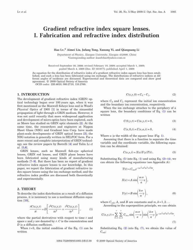
here a is the width of the square lens (Fig. 1).Assuming that there is a function to separate the time

ariable and the coordinate variable, the following equa-ion can be obtained:

C�x,y,t� = X�x�Y�y�T�t�. �5�

ubstituting Eq. (5) into Eq. (1) and using Eq. (2)–(4), wean obtain the following equations (see Appendix A):

T�t� = Cmne−�m2+k2/a2��2Dt,

X�x� = A sin�m�

ax� ,

Y�y� = B sin�k�

ay� , �6�

here Cmk, A, and B are constants and m ,k=1,2. . ..According to the superposition principle, we can obtain

C�x,y,t� = �k=1

�

�m=1

�

Cmn sin�m�

ax�sin�k�

ay�e−�m2+k2/a2��2Dt.

�7�

ubstituting Eq. (2) into Eq. (7), we obtain the value of:

mk

009 Optical Society of America

At

ctd

Ce

et

r

w

3SpALcw1chpag

e(itT

Ff

1086 J. Opt. Soc. Am. A/Vol. 26, No. 5 /May 2009 Lv et al.

Cmk =4

a2�0

a�0

a

sin�m�

ax�sin�k�

ay�dxdy. �8�

ccordingly, substituting Eq. (8) into Eq. (7), the concen-ration difference �C of exchanging ions can be obtained:

�C = C�x,y,t� − C1

= �k=1

�

�m=1

�

Cmk sin�m�

ax�sin�k�

ay�e−�m2+k2/a2��2Dt.

�9�

In ion exchange, the driving force of the diffusion pro-ess is the concentration gradient of the dopant ion, andhe dopant distribution will result from Fickian diffusionescribed by [8]

�n�x,y,t�

�t= D� �2n�x,y,t�

�x2 +�2n�x,y,t�

�y2 � . �10�

omparing Eq. (10) with Eq. (1), one can see there is a lin-ar relationship between the refractive index and the ion

ig. 1. (Color online) Design schematic diagram of gradient re-ractive index square lens.

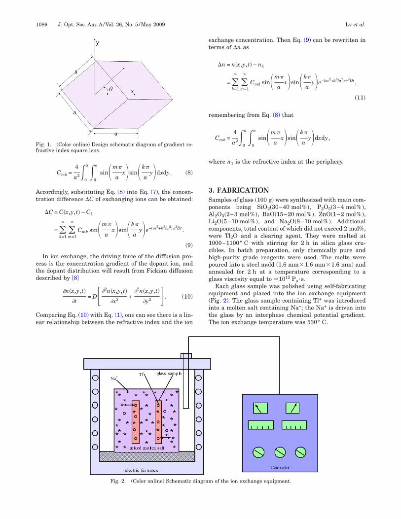
Fig. 2. (Color online) Schematic d

xchange concentration. Then Eq. (9) can be rewritten inerms of �n as

�n = n�x,y,t� − n1

= �k=1

�

�m=1

�

Cmk sin�m�

ax�sin�k�

ay�e−�m2+k2/a2��2Dt,

�11�

emembering from Eq. (8) that

Cmk =4

a2�0

a�0

a

sin�m�

ax�sin�k�

ay�dxdy,

here n1 is the refractive index at the periphery.

. FABRICATIONamples of glass �100 g� were synthesized with main com-onents being SiO2�30–40 mol% �, P2O5�3–4 mol% �,l2O3�2–3 mol% �, BaO�15–20 mol% �, ZnO�1–2 mol% �,i2O�5–10 mol% �, and Na2O�8–10 mol% �. Additionalomponents, total content of which did not exceed 2 mol%,ere Tl2O and a clearing agent. They were melted at000–1100° C with stirring for 2 h in silica glass cru-ibles. In batch preparation, only chemically pure andigh-purity grade reagents were used. The melts wereoured into a steel mold �1.6 mm�1.6 mm�1.6 mm� andnnealed for 2 h at a temperature corresponding to alass viscosity equal to 1012 Pa·s.

Each glass sample was polished using self-fabricatingquipment and placed into the ion exchange equipmentFig. 2). The glass sample containing Tl+ was introducednto a molten salt containing Na+; the Na+ is driven intohe glass by an interphase chemical potential gradient.he ion exchange temperature was 530° C.

of the ion exchange equipment.

iagram

4TPfufc

w

wafmcTOclt

tv6pret

5Tssm

F=

Lv et al. Vol. 26, No. 5 /May 2009/J. Opt. Soc. Am. A 1087

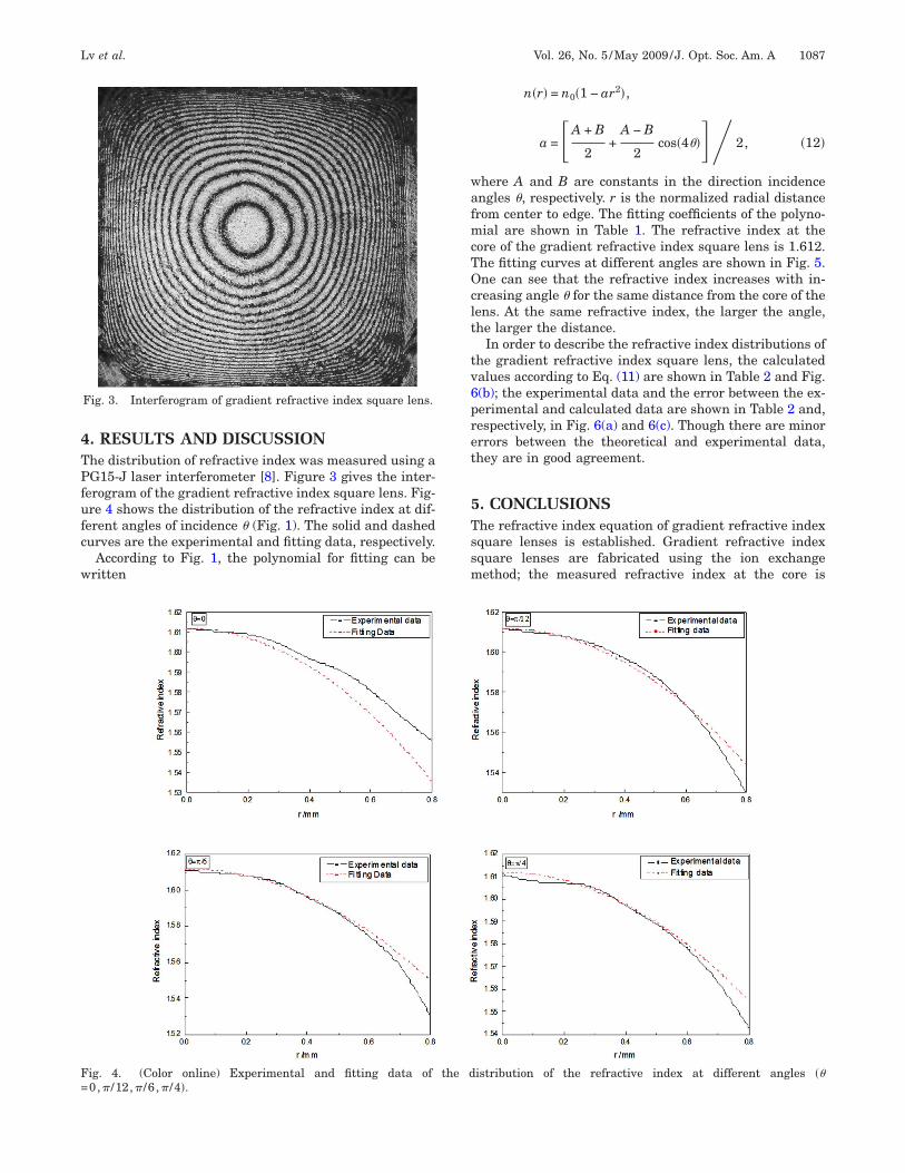
. RESULTS AND DISCUSSIONhe distribution of refractive index was measured using aG15-J laser interferometer [8]. Figure 3 gives the inter-

erogram of the gradient refractive index square lens. Fig-re 4 shows the distribution of the refractive index at dif-erent angles of incidence � (Fig. 1). The solid and dashedurves are the experimental and fitting data, respectively.

According to Fig. 1, the polynomial for fitting can beritten

Fig. 3. Interferogram of gradient refractive index square lens.

ig. 4. (Color online) Experimental and fitting data of0,� /12,� /6 ,� /4�.

n�r� = n0�1 − ar2�,

a = �A + B

2+

A − B

2cos�4��� 2, �12�

here A and B are constants in the direction incidencengles �, respectively. r is the normalized radial distancerom center to edge. The fitting coefficients of the polyno-ial are shown in Table 1. The refractive index at the

ore of the gradient refractive index square lens is 1.612.he fitting curves at different angles are shown in Fig. 5.ne can see that the refractive index increases with in-

reasing angle � for the same distance from the core of theens. At the same refractive index, the larger the angle,he larger the distance.

In order to describe the refractive index distributions ofhe gradient refractive index square lens, the calculatedalues according to Eq. (11) are shown in Table 2 and Fig.(b); the experimental data and the error between the ex-erimental and calculated data are shown in Table 2 and,espectively, in Fig. 6(a) and 6(c). Though there are minorrrors between the theoretical and experimental data,hey are in good agreement.

. CONCLUSIONShe refractive index equation of gradient refractive indexquare lenses is established. Gradient refractive indexquare lenses are fabricated using the ion exchangeethod; the measured refractive index at the core is

istribution of the refractive index at different angles ��

the d

actdCiri

ASi

Fd

A ]

Ft

1088 J. Opt. Soc. Am. A/Vol. 26, No. 5 /May 2009 Lv et al.

1.612. The refractive index distribution at differentngles of viewing are discussed. The refractive index in-reases with increasing viewing angle at the same dis-ance from the core of the lens. At the same refractive in-ex, the larger the viewing angle, the larger the distance.omparing the experimental and theoretical data, there

s good agreement, though there are minor errors. Thisesearch is a basis for future study of gradient refractivendex square lens arrays.

PPENDIX Aubstituting Eq. (5) into Eqs. (1), (3), and (4), the follow-

ng equations can be obtained:

Table 2. Theoretical, Experimental Data, andError of Gradient Refractive Index Square Lens

Coordinates�x ,y� Experimental Data Theoretical Data Error

(1.131,1.000) 1.6142 1.6127 0.093(1.525,1.000) 1.5844 1.5798 0.290(1.511,1.137) 1.5840 1.5813 0.170(1.657,1.176) 1.5612 1.5561 0.330(1.065,1.113) 1.6141 1.6127 0.087(1.272,1.471) 0.5844 1.5838 0.004(1.093,1.093) 1.6145 1.6127 0.011(1.391,1.391) 1.5844 1.5854 0.063(1.535,1.535) 1.5613 1.5624 0.070

ig. 5. (Color online) Fitting curves of the refractive index atifferent angles ��=0,� /12,� /6 ,� /4�.

Table 1. Optimized Coefficients for the RefractiveIndex Profile

ngle ���Fitting

Coefficient �a� Polynomial [n�r�=n0�1−ar2�, n0=1.612

0 0.0659 n�r�=n0�1−0.0659r2�� /12 0.1188 n�r�=n0�1−0.1188r2�� /6 0.0968 n�r�=n0�1−0.0968r2�� /4 0.0890 n�r�=n0�1−0.0890r2�

T�

DT−

X�

X−

Y�

Y= 0, �A1�

X�0�Y�y�T�t� = X�a�Y�y�T�t� = 0, �A2�

ig. 6. (Color online) Results diagram of Table 2: (a) experimen-al data, (b) theoretical data, (c) error.

It

Ut

a

St

ATE

R

1

Lv et al. Vol. 26, No. 5 /May 2009/J. Opt. Soc. Am. A 1089

X�x�Y�0�T�t� = X�x�Y�a�T�t� = 0, �A3�

X�x�Y�y�T�0� = C0 − C1. �A4�

n order to obtain the solution of Eq. (A1), we assume thathere are functions

X� + EX = 0,

Y� + FX = 0. �A5�

sing the initial conditions, X�0�=X�a�=0, Y�0�=Y�a�=0,he values of the constants E and F can be calculated as

E = �m��2/a2,

F = �k��2/a2, �A6�

nd the solutions of Eq. (A5) can be obtained as

X�x� = A sin�m�

ax� ,

Y�y� = B sin�k�

ay� . �A7�

ubstituting Eqs. (A5)–(A7) into Eq. (A1), we can obtainhe value of T�t�

T�t� = C e−�m2+k2/a2��2Dt. �A8�

mk

CKNOWLEDGMENTShis work is supported by the Research Foundation ofducation Bureau of Hubei Province, China.

EFERENCES1. R. W. Wood, Physical Optics (MacMillan, 1905).2. D. T. Moore, “Gradient-index optics: a review,” Appl. Opt.

19, 1035–1038 (1980).3. K. Iga, “Theory for gradient-index imaging,” Appl. Opt. 19,

1039–1043 (1980).4. N. F. Borrell, Micro-optics Technology (Marcel Dekker,

1999).5. Y. L. Li, W. P. Wang, X. D. Zhang, and J. M. Huo,

“Preparations on several GRIN lenses,” Acta Opt. Sin. 23,23–24 (2003) (in Chinese).

6. Y. L. Li, T. H. Li, G. H. Jiao, B. W. Hu, J. M. Huo, and L. L.Wang, “Research on micro-optical lenses fabricationtechnology,” Optik (Stuttgart) 118, 395–401 (2007).

7. S. Ilyas and M. Gal, “Gradient refractive index planarmicrolens in Si using porous silicon,” Appl. Phys. Lett. 89,211123–211125 (2006).

8. H. Lv, B. Shi, L. Guo, and A. Liu, “Fabrication of Maxwellfish-eye spherical lenses and research on distributionprofiles of gradient refractive index,” J. Opt. Soc. Am. A 25,609–611 (2008).

9. K. Fujii, S. Ogi, and N. Akazawa, “Gradient-index rod lenswith a high acceptance angle for color use by Na+ for Li+

exchange,” Appl. Opt. 33, 8087–8093 (1994).0. B. Messerschmidt, B. L. McIntyre, and S. N. Houde-Walter,

“Desired concentration-dependent ion exchange for micro-optic lenses,” Appl. Opt. 35, 5670–5676 (1996).