1

Gradient Wind Adjustment and Tropical Cyclone Intensification

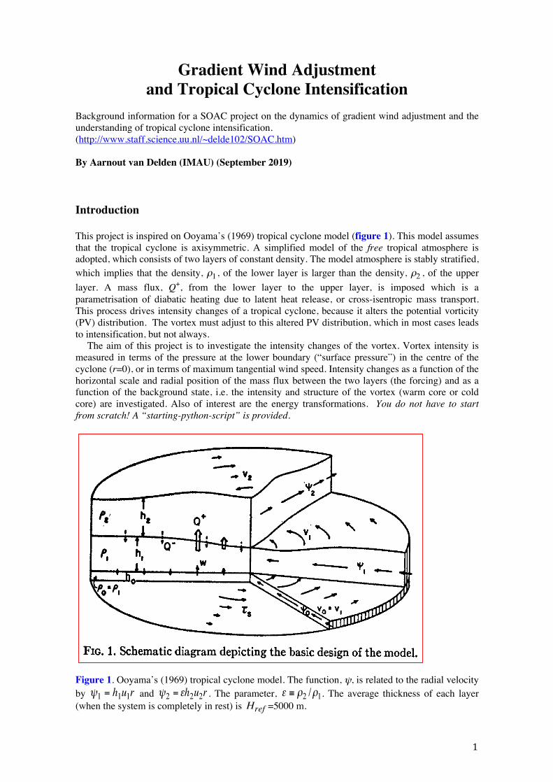
Background information for a SOAC project on the dynamics of gradient wind adjustment and the understanding of tropical cyclone intensification. (http://www.staff.science.uu.nl/~delde102/SOAC.htm) By Aarnout van Delden (IMAU) (September 2019) Introduction This project is inspired on Ooyama’s (1969) tropical cyclone model (figure 1). This model assumes that the tropical cyclone is axisymmetric. A simplified model of the free tropical atmosphere is adopted, which consists of two layers of constant density. The model atmosphere is stably stratified, which implies that the density, ρ1 , of the lower layer is larger than the density, ρ2 , of the upper layer. A mass flux, Q+, from the lower layer to the upper layer, is imposed which is a parametrisation of diabatic heating due to latent heat release, or cross-isentropic mass transport. This process drives intensity changes of a tropical cyclone, because it alters the potential vorticity (PV) distribution. The vortex must adjust to this altered PV distribution, which in most cases leads to intensification, but not always. The aim of this project is to investigate the intensity changes of the vortex. Vortex intensity is measured in terms of the pressure at the lower boundary (“surface pressure”) in the centre of the cyclone (r=0), or in terms of maximum tangential wind speed. Intensity changes as a function of the horizontal scale and radial position of the mass flux between the two layers (the forcing) and as a function of the background state, i.e. the intensity and structure of the vortex (warm core or cold core) are investigated. Also of interest are the energy transformations. You do not have to start from scratch! A “starting-python-script” is provided.

Figure 1. Ooyama’s (1969) tropical cyclone model. The function, ψ, is related to the radial velocity by

€

ψ1 = h1u1r and

€

ψ2 = εh2u2r . The parameter,

€

ε ≡ ρ2 /ρ1. The average thickness of each layer (when the system is completely in rest) is

€

Href =5000 m.

2

Governing equations

The equations, which govern the tangential (v) and radial (u) velocity components and the thickness (h) of the two upper layers, are

€

∂rvi∂t

+ ui∂rvi∂r

= −rfui , (1)

€

∂ui∂t

+ ui∂ui∂r

= −∂Φi∂r

+ vi f +vir

⎛

⎝ ⎜

⎞

⎠ ⎟ , (2)

€

∂hi∂t

+ ui∂hi∂r

= −hir∂rui∂r

+ Mi . (3)

The subscript, i, indicates the index of the layer. Layer, i=1, is the lower layer in the free troposphere. Layer, i=2, is the upper layer in the free troposphere. For simplicity, we neglect the existence of the lower boundary layer (layer 0). The geopotential, Φ, is related to the thickness of the layers by

€

Φ1 = g h1 +εh2 − z( ) and

€

Φ2 = g h1 + h2 − z( ) , (4) with

€

ε =ρ2ρ1

<1 . (5)

The mass flux between the two layers is a parametrisation of latent heat release due to condensation in clouds, which is hypothesized to drive tropical cyclone intensification. If upward (positive), this mass flux increases the thickness of the upper layer at the cost of the thickness of the lower layer, which qualitatively has the correct influence on the potential vorticity. In other words, potential vorticity increases below the heat source and decreases above the heat source. The (diabatic) mass flux can be prescribed as

€

M1 = −Qexp −r − r0( )2

a2

⎧ ⎨ ⎪

⎩ ⎪

⎫ ⎬ ⎪

⎭ ⎪ , (6)

€

M2 =Qεexp −

r − r0( )2

a2

⎧ ⎨ ⎪

⎩ ⎪

⎫ ⎬ ⎪

⎭ ⎪ , (7)

so that

€

M1 +εM2 = 0 . (8) Q,

€

r0 and a are parameters to be prescribed, representing the amplitude and the horizontal scale of the mass flux, respectively. The parameter, Q, may be a linear function of time:

€

Q =Q0T

if t ≤ T and Q = 0 if t > T . (9)

€

Q0 is a prescribed constant. We will investigate the response of the system as a function of the times scale, T, and the spatial scale, a, of the forcing (the mass flux between the two layers).

3

Numerical solution of the time-dependent linear problem We first solve equations (1) to (3), linearised around the state of rest:

€

∂vi∂t

= − fui , (10)

€

∂ui∂t

= −∂Φi∂r

+ vi f +vir

⎛

⎝ ⎜

⎞

⎠ ⎟ , (11)

€

∂hi∂t

= −Hrefr

∂rui∂r

+ Mi . (12)

We use a stretched grid in the radial direction, which is given by

€

r x( ) = b exp λx( ) −1{ } with x = 0,1,2,... (13) If x=0, r=0. The grid spacing in x, Δx=1. The values of the parameters, b and λ, can be tuned to obtain the desired resolution and stretching. In the example shown here, b=20000 and λ=0.05. Derivatives with respect to r must be expressed as derivatives with respect to x using

€

∂∂r

=dxdr

∂∂x

(14)

with

€

dxdr

=1

λ r + b( ) or

€

dr = λ r + b( )dx . (15)

The boundary condition at r=0 is as follows:

€

u = v =∂h∂r

=∂Φ∂r

= 0 .

Eq. (12) is solved at integer values of x, i.e. at x=0,1, 2, 3,… (eq. 13) and eqs. (1) and (2) are solved at points half way these points (i.e. at x=0.5, 1.5, 2.5,…). Figure 2 shows the final state, in terms of the tangential velocities and the gradient wind velocities in both layers of an integration, starting from the state of rest, in which ε=0.9, a=500 km.

€

r0=0, T=6 hours,

€

Q0=0.2x

€

Href and

€

Href =5000 m. The approximation of the time derivative is Euler forward in the predictor step and Euler backward in the corrector step. The new values of h and v from the predictor step are used directly for the “predictor step” of eq. (11) (the eq. for ∂u/∂t). The new value of u is used to recalculate the new values of h and v (corrector step). The scheme, therefore, is semi-implicit and appears to be numerically stable if the initial state corresponds to the state of rest. The system will tend to adjust to gradient wind balance:

€

v f +vr

⎛

⎝ ⎜

⎞

⎠ ⎟ =

∂Φ∂r , (16)

which is the steady state solution of (11) (for simplicity, we have dropped the subscript i). Eq. 16 can solved for v.This yields the gradient wind (

€

vgrad ) equation:

€

vgrad = −fr2

±12

f 2r2 + 4r ∂Φ∂r

, (17)

4

Figure 2. Tangential velocities in both layers at t=24 hours (upper panel) and at t=36 hours (lower panel) as a function radius in an integration of the linear shallow water equations (i.e. linearised around the initial steady state of rest). The initial state is the state of rest. Also plotted is the gradient wind (thin curves). Parameter values are ε=0.9, a=500 km, T=6 hours (eq. 9) and Q0= 0.2x

€

Href=1000 m. The thick lines correspond to the real velocity, while the thin lines correspond to the gradient velocity (eq. 10). The internal Rossby radius (eq. 16) in this case is 700 km. The surface pressure at r=0 has decreased by 1.43 hPa between t=0 and t=36 hrs. Oscillations are still present both at t=24 hrs and at t=36 hrs, which induce deviations from gradient wind balance.

5

Eq. 17 has a solution if

€

∂Φi∂r

≥ −f 2r4g (18)

The model is initialized with the state of rest. After 36hours (figure 2, lower panel) a weak nearly balanced cyclonic vortex is observed in the lower layer (max tangential wind velocity is 1.83 m/s) while a weak nearly balanced anti-cyclonic vortex is observed in the upper layer (minimum tangential wind velocity is -2.09 m/s). Imbalances are clearly visible at t=24 hrs at r>1000 km. These imbalances propagate outward and represent gravity inertia waves. Numerical solution of the “quasi-nonlinear” problem It will also be possible to initialise the model with a finite amplitude vortex in gradient wind balance. We can then investigate the vortex intensity changes, due to the mass flux, M, as function of vortex intensity and structure. Initially, a balanced “Rankine vortex” is prescribed. The tangential wind in a Rankine vortex is given by,

€

v r( ) =vmaxrRmax

if r ≤ Rmax; v r( ) =vmaxRmax

r if r > Rmax . (19)

Here,

€

vmax is the prescribed maximum tangential velocity, which need not be equal in both layers. In fact, the vertical shear of the tangential wind speed determines whether a balanced cyclone is “warm-core”, “cold-core” or “barotropic”. A warm core balanced cyclone is characterised by a decrease of the tangential wind with height (

€

v1>

€

v2). It has been shown by van Delden (1989) that a warm core cyclone responds much more strongly to a given forcing (mass flux) than a cold-core vortex. We now linearise the equations around the finite amplitude vortex, which leads to the following set of governing equations.

€

∂vi∂t

= −ui f +ζi( ), (19)

€

∂ui∂t

= −ui∂ui∂r

−∂Φi∂r

+ vi f +vir

⎛

⎝ ⎜

⎞

⎠ ⎟ ≈ −

∂Φi∂r

+ vi f +vir

⎛

⎝ ⎜

⎞

⎠ ⎟ , (20)

€

∂hi∂t

= −1r∂rhiui∂r

+ Mi ≈ −Href

r∂rui∂r

+ Mi . (21)

where

€

ζi =1r∂rvi∂r

. (22)

We have also assumed that the term, u∂u/∂r, in eq. 20 can be neglected and that

€

hi ≈ Href in eq. 21. Initially, in both layers,

€

ζ =2vmaxRmax

if r ≤ Rmax; ζ = 0 if r > Rmax . (23)

6

Figure 3. Tangential velocities in both layers as a function radius at t=18 hours in two integrations with a finite amplitude Rankine vortex as initial condition. (1) (upper panel) with

€

vmax = 30 m/s in layer 1 and vmax =15 m/s in layer 2 (a baroclinic “warm core” vortex); (2) (lower panel) with

€

vmax =15 m/s in layer 1 and vmax = 30 m/s in layer 2 (a baroclinic “cold core” vortex). The radius of maximum wind is 500 km in both layers. Also plotted is the gradient wind (thin curves). Parameter values are ε=0.9, a=500 km, T=6 hours (eq. 9) and Q0= 0.2x

€

Href =1000 m. The thick lines correspond to the real velocity, while the thin lines correspond to the gradient velocity (eq. 10). The internal Rossby radius (eq. 16) in this case is 318 km. In the first case the surface pressure at r=0 decreases by 3.1 hPa between t=0 and t=18 hrs (see figure 4). In the second case the surface pressure at r=0 decreases by 1.9 hPa between t=0 and t=18 hrs. In other words, the same mass flux has a much larger effect on central surface pressure if the vortex is intense and has a “warm core”.

7

Figure 4. Central (r=0) surface pressure deficit (relative to the initial state) as a function of time in the simulation starting with a warm-core vortex (upper panel of figure 3). At later times we assume that

€

ζ =1r∂rvgrad∂r

. (24)

where

€

vgrad (eq. 17) is calculated at the same gridpoints as h (i.e. at x=0,1,2,3…) using a centred difference approximation, so that the relative vorticity is obtained on the same intermediate grid points as u and v. The results of two integrations are shown in figure 3. Both integrations are initialised with a finite amplitude Rankine vortex in gradient wind balance. In the upper panel the initial state is a “warm-core” vortex in which the balanced wind velocity decreases with height, i.e.

€

v1 > v2. In the lower panel the initial state is a “cold-core” vortex with

€

v2 > v1. The vortex is nearly perfectly in gradient wind balance at t=18 hrs, but note the initial stage of what is presumably a numerical instability near r=0. This, apparently, does not (yet) affect the central surface pressure (figure 4). Research questions (0) Investigate the boundary condition at r=0. Try to solve the numerical problem that is visible in figure 3? (1) Analyse the dynamics of the inertia-gravity waves, which propagate to larger r, in an experiment in which the forcing-time, T (eq. 9), is shorter than 6 hours. Do the waves have any effect on the potential vorticity distribution? (2) Investigate the dependence of the central surface pressure tendency on the structure and scale of the initial balanced vortex for different diabatic mass flux distributions. For example, you may try to find out what happens when the diabatic mass flux is located out side the radius of maximum wind (

€

r0 ≠ 0). (3) Find the final balanced state from potential vorticity inversion . (4) The gradient wind balance equation (17) has two solutions. The normal state of gradient wind balance, when ∂Φ/∂r>0, is the solution with the plus sign in front of the square root on the r.h.s. of eq. 17, which corresponds to a cyclonic circulation (v>0). The solution with minus sign in front of the square root corresponds to an anticyclonic circulation (v<0). Try to initialize the model with the latter solution.

8

Literature Aarnout van Delden, 2017: Chapter 5 of the lecture notes on Atmospheric Dynamics. http://www.staff.science.uu.nl/~delde102/AtmosphericDynamics.htm . Aarnout van Delden, 1989: On the deepening and filling of balanced cyclones by diabatic heating. Meteorol.Atmos.Phys., 41, 127-145. pdf Allen C. Kuo and Lorenzo M. Polvani, 2000: Nonlinear geostrophic adjustment, cyclone/anticyclone asymmetry and potential vorticity rearrangement. Physics of Fluids, 12, 1087-1100. Katsuyuki Ooyama, 1969: Numerical simulation of the life-cycle of tropical cyclones. J.Atmos.Sci., 26, 3-40. David Randall, 1994: Geostrophic adjustment and the finite difference shallow water equations. J.Atmos.Sci., 122, 1371-1377. Rick Salmon, 1998: Lectures on Geophysical Fluid Dynamics. Oxford University Press. Page 90-91.