Graduate Public Finance - Overview of Public Finance...

Graduate Public FinanceOverview of Public Finance in a Spatial Setting

Owen ZidarUniversity of Chicago

Introduction

Graduate Public Finance Overview of Spatial Public Finance Introduction 1 / 35

Outline

1 Introductions: logistics, schedule, etc

2 Motivation and Goals

3 What is special about spatial public finance?

4 Main Questions

5 Course Outline


Introductions: who am I/ who are you?

1 My backgroundPh.D. from UC Berkeley, BA from DartmouthStaff Economist at Council of Economic Advisers

2 Research fiscal policy topicsIncidence and efficiency costs of corporate taxationEconomic impacts of taxing high-income earnersEffect of state tax system on U.S. economyThe structure of state corporate taxationBusiness taxation and ownership in the U.S.Who profits from patents? Rent sharing at innovative firmsBusiness Income and U.S. income inequality


Motivation and Goals

Motivation:

1 Key policy debates, large spatial disparities, labs of democracy

2 Rich setting for economics and great data

3 Overlap w/ many fields (labor, urban, trade, development, macro)

Goals:

1 Provide context and guidance on open questions

2 Present benchmark models and new research

3 Enhance your applied modeling and empirical skills


What’s special about Spatial PF?

Mobility of factors (and goods)

Spillovers

AgglomorationCongestion

Spatial Heterogeneity in Endowments (and Outcomes)

Hierarchy

FederalismCompetition with many neighbors


Questions

1 Taxation: how should we pay for government services?What should we tax? With what structure? At what rate?Taxation of capital, labor, and goods in a spatial settingIncidence, efficiency, and policy implications

2 Spending: how big should government be and what should it provide?

Are local services being under or over provided (level and composition)?How are local services allocated? E.g., How much police spendingallocated to rich/poor neighborhoods?Redistribution, safety net, and mobility responses to benefit generosity

3 Hierarchy: How should governments be organized?When is local provision efficient?Fiscal federalism and Tax Competition

4 Dynamics: Growth, Economic Development, and PovertyBig push and Industrial policy? Local vs Aggregate Consequences?Should we have special economic zones? Bail outs? Pension reform?Opportunity and growth across locations: causes, consequences, andpolicy implications


Course Outline

1 Overview, baseline Rosen-Roback spatial model

2 Place-based Policies and Spatial Disparities in Opportunity1 Welfare Economics of Local Economic Development Programs2 Where is the Land of Opportunity

3 Capital taxes in a spatial setting, the Harberger Model1 Brief overview of capital taxation2 Capital Taxes with Two Sectors (corporate taxes and property taxes)

4 Firm Location and Taxes, Million Dollar Plants, Agglomeration1 Firm Location and Taxes2 Million Dollar Plants3 Big Push and Agglomeration in Production, Consumption (and Public

Goods)


Graduate Public FinanceThe Rosen-Roback Spatial Model1

Owen ZidarUniversity of Chicago

Lecture 1

1Thanks to David Card for providing his lecture notes, some of which are reproducedand extended here. Stephanie Kestelman provided excellent assistance making theseslides.

Graduate Public Finance Rosen-Roback Spatial Model Lecture 1 8 / 35

Outline

1 ModelOverviewWorkers: Indirect Utility ConditionFirms: No Profit Condition

2 EquilibriumComponents of Economic ModelsExogenous Model ParametersEndogenous Model OutcomesEquilibrium: Indifference ConditionsSolving Model

3 Comparative Statics and Value of AmenitiesPrice effects under different assumptions about amenitiesInferring Amenity ValuesExtensions (Albouy JPE, 2009)


Outline





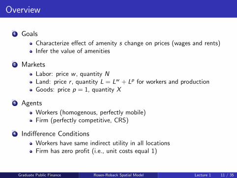
Overview

1 Goals

Characterize effect of amenity s change on prices (wages and rents)Infer the value of amenities

2 Markets

Labor: price w , quantity NLand: price r , quantity L = Lw + Lp for workers and productionGoods: price p = 1, quantity X

3 Agents

Workers (homogenous, perfectly mobile)Firm (perfectly competitive, CRS)

4 Indifference Conditions

Workers have same indirect utility in all locationsFirm has zero profit (i.e., unit costs equal 1)


Workers: Preferences and Budget Constraint

Utility is u(x , lc , s)

x is consumption of private good

lc is consumption of land

s is amenity

Budget constraint is x + rlc − w − I = 0

I is non-labor income that is independent of location (e.g., share ofnational land portfolio)

w is labor income (note: no hours margin).


Workers: Indirect Utility

Indirect utility is given

V (w , r , s) = maxx ,lc

u(x , lc , s) s.t. x + rlc − w − I = 0

Let λ = λ(w , r , s) be the marginal utility of a dollar of income, then

Vw = λ > 0

Vr = −λlc < 0

⇒ Vr = −Vw lc


Aside: Example of Indirect Utility

Utility is Cobb Douglas over goods and land with an amenity shifter:

u(x , lc , s) = sθW xγ(lc)1−γ

Then x = γ(w+I1

)and lc = (1− γ)

(w+Ir

)So indirect utility is:

V (w , r , s) = γγ(1− γ)(1−γ)︸︷︷︸constant

sθW︸︷︷︸Amenities

1−γr−(1−γ)︸︷︷︸Prices

(w + I )︸︷︷︸Income

MU of income is λ(w , r , s)

Vw = λ = γγ(1− γ)(1−γ)sθW 1−γr−(1−γ)

Vr = −λlc = −γγ(1− γ)(1−γ)sθW 1−γr−(1−γ) (1− γ)

(w + I

r

)︸︷︷︸

lc

⇒ Vr = −Vw lc


Firms: Unit Cost Function

CRS production with cost function C (X ,w , r , s)

X is output

Unit cost c(w , r , s) = C(X ,w ,r ,s)X

Lp is total amount of land used by firms

N is total employment

From Sheppard’s Lemma, we have

cw = N/X > 0

cr = Lp/X > 0


Aside: Example technology, cost function, factor demand

Suppose X = f (N, Lp) = sθFNαL1−α, then cost function is:

C (X ,w , r , s) = X (sθF )−1wαr1−α(α−α(1− α)−(1−α))⇒c(w , r , s) = (sθF )−1wαr1−α(α−α(1− α)−(1−α))

Then

Cw (X ,w , r , s) = α

(X (sθF )−1wαr1−α(α−α(1− α)−(1−α))

)w

= N

Cr (X ,w , r , s) = (1− α)

(X (sθF )−1wαr1−α(α−α(1− α)−(1−α))

)r

= Lp

Dividing both sides by X gives:

cw = N/X > 0

cr = Lp/X > 0


Outline





Aside: Components of Models2

Three parts of any model

1 Exogenous parameters: model elements that are taken “as given”

2 Endogenous outcomes: model elements that “move around”

3 Equilibrium conditions: the set of rules that tells you what theendogenous model outcomes should be for a given set of exogenousmodel parameters.

“Given a [insert set of exogenous model parameters here], equilibrium isdefined by the [insert endogenous model outcomes here] such that [listequilibrium conditions here].”

2Follows Treb Allen’s NotesGraduate Public Finance Rosen-Roback Spatial Model Lecture 1 18 / 35

Exogenous parameters

Workers Parameters: s, θW , γ, I

s is level of amenitiesθW governs importance of amenities for utilityγ governs importance of goods for utility1− γ governs importance of land for utilityI is non-labor income

Firm Parameters: s, θF , α

s is level of amenitiesθF governs importance of amenities for productivityα is output elasticity of labor1− α is output elasticity of land


Endogenous Model Outcomes

Recall:

Labor: price w , quantity N

Land: price r , quantities Lw , Lp for workers and production

Goods: price p = 1, quantity X

so endogenous outcomes are w , r ,N, Lw , Lp,X


Equilibrium Concept: Two key indifference conditions

In equilibrium, workers and firms are indifferent across cities with differentlevels of s and endogenously varying wages w(s) and rents r(s):

c(w(s), r(s), s) = 1 (1)

V (w(s), r(s), s) = V 0 (2)

where V 0 is the initial equilibrium level of indirect utility.

Specifically, in our example:Given s, θW , θF , γ, I , α, equilibrium is defined by local prices and quantitiesw , r ,N, Lw , Lp,X such that 1 and 2 hold and land markets clear.

N.B. We will mainly be focusing on prices: w(s) and r(s).


Solving for effect of amenity changes on prices

Differentiate 1 and 2 with respect to s and rearrange, we have:[cw crVw Vr

] [w ′(s)r ′(s)

]=

[−cs−Vs

](3)

Solving for w ′(s), r ′(s), we have

w ′(s) =Vrcs − crVs

crVw − cwVr

r ′(s) =Vscw − csVw

crVw − cwVr

Note we can rewrite

crVw − cwVr = λLp/X + λlcN/X = λL/X = VwL/X


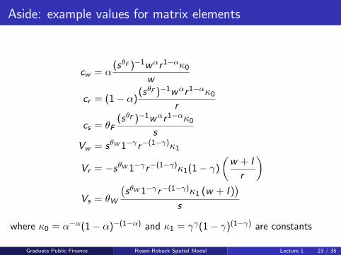
Aside: example values for matrix elements

cw = α(sθF )−1wαr1−ακ0

w

cr = (1− α)(sθF )−1wαr1−ακ0

r

cs = θF(sθF )−1wαr1−ακ0

s

Vw = sθW 1−γr−(1−γ)κ1

Vr = −sθW 1−γr−(1−γ)κ1(1− γ)

(w + I

r

)Vs = θW

(sθW 1−γr−(1−γ)κ1 (w + I )

)s

where κ0 = α−α(1− α)−(1−α) and κ1 = γγ(1− γ)(1−γ) are constants


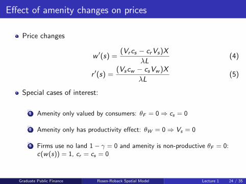
Effect of amenity changes on prices

Price changes

w ′(s) =(Vrcs − crVs)X

λL(4)

r ′(s) =(Vscw − csVw )X

λL(5)

Special cases of interest:

1 Amenity only valued by consumers: θF = 0⇒ cs = 0

2 Amenity only has productivity effect: θW = 0⇒ Vs = 0

3 Firms use no land 1− γ = 0 and amenity is non-productive θF = 0:c(w(s)) = 1, cr = cs = 0


Outline





1. Amenity only valued by consumers: θF = 0⇒ cs = 0

When cs = 0, higher s ⇒ higher r , lower l

Workers are willing to pay more in land rents and receive less in payto have access to higher levels of amenities

w

r

V(w, r, s0) = V0

V(w, r, s1) = V0

c(w, r) = 1


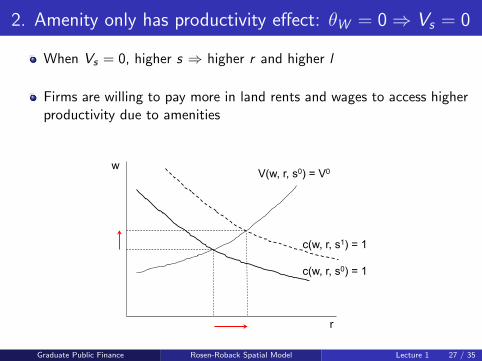
2. Amenity only has productivity effect: θW = 0⇒ Vs = 0

When Vs = 0, higher s ⇒ higher r and higher l

Firms are willing to pay more in land rents and wages to access higherproductivity due to amenities

w

r

V(w, r, s0) = V0

c(w, r, s0) = 1

c(w, r, s1) = 1


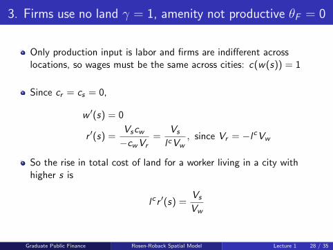
3. Firms use no land γ = 1, amenity not productive θF = 0

Only production input is labor and firms are indifferent acrosslocations, so wages must be the same across cities: c(w(s)) = 1

Since cr = cs = 0,

w ′(s) = 0

r ′(s) =Vscw−cwVr

=Vs

lcVw, since Vr = −lcVw

So the rise in total cost of land for a worker living in a city withhigher s is

lc r ′(s) =Vs

Vw


3. Firms use no land γ = 1, amenity not productive θF = 0

VsVw

= marginal WTP for a change in s so the marginal value of achange in the amenity is “fully capitalized” in rents

w

r

V(w, r, s0) = V0

c(w, s0) = 1

V(w, r, s1) = V1

VsVw

= θW(w+I )

s is increasing in income, decreasing in level of amenities


Inferring the Value of Amenities

How do we infer the value of amenities in the more general case?

Ω(s) = V (w(s), r(s), s) represents total utility of living in city s

If all cities have equal utility, then

Ω′(s) = Vww′(s) + Vr r

′(s) + Vs = 0 in equilibrium

Vs = −Vww′(s)− Vr r

′(s)

Vs = −Vww′(s) + lcVw r

′(s)

⇒ Vs

Vw= lc r ′(s)− w ′(s) (6)

So WTP for the amenity is extra land cost for consumers less lowerwages in a higher-amenity city


Inferring the Value of Amenities

We can get more insight from looking at firms:

Firms face c(w(s), r(s), s) = 1 across cities, so

cww′(s) + cr r

′(s) + cs = 0 (7)

Consider 2 cases

1 cs = 0 (no productivity effects of higher amenity levels)

2 cs 6= 0


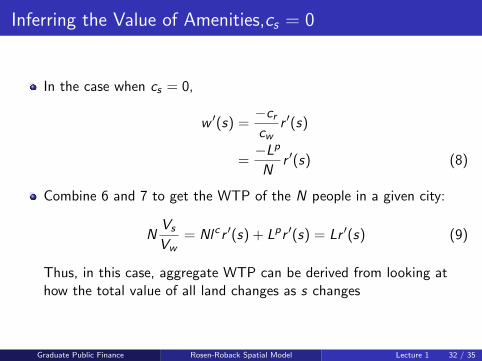
Inferring the Value of Amenities,cs = 0

In the case when cs = 0,

w ′(s) =−crcw

r ′(s)

=−Lp

Nr ′(s) (8)

Combine 6 and 7 to get the WTP of the N people in a given city:

NVs

Vw= Nlc r ′(s) + Lpr ′(s) = Lr ′(s) (9)

Thus, in this case, aggregate WTP can be derived from looking athow the total value of all land changes as s changes


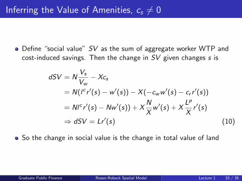
Inferring the Value of Amenities, cs 6= 0

Define “social value” SV as the sum of aggregate worker WTP andcost-induced savings. Then the change in SV given changes s is

dSV = NVs

Vw− Xcs

= N(lc r ′(s)− w ′(s))− X (−cww ′(s)− cr r′(s))

= Nlc r ′(s)− Nw ′(s)) + XN

Xw ′(s) + X

Lp

Xr ′(s)

⇒ dSV = Lr ′(s) (10)

So the change in social value is the change in total value of land


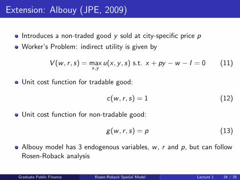
Extension: Albouy (JPE, 2009)

Introduces a non-traded good y sold at city-specific price p

Worker’s Problem: indirect utility is given by

V (w , r , s) = maxx ,y

u(x , y , s) s.t. x + py − w − I = 0 (11)

Unit cost function for tradable good:

c(w , r , s) = 1 (12)

Unit cost function for non-tradable good:

g(w , r , s) = p (13)

Albouy model has 3 endogenous variables, w , r and p, but can followRosen-Roback analysis


Extension: Albouy (JPE, 2009)

Studies the unequal geographic burden of federal taxation

Progressive fed tax schedule ⇒ higher taxes in higher w places

“Federal taxes act like an arbitrary head tax for living in a city withwage improving attributes, whatever those attributes may be”

Simulation: a worker moving from a typical low-wage city to ahigh-wage city would experience a 27% increase in federal taxes,which is equivalent to a $269 billion transfer from workers inhigh-wage, high-productivity areas to low-wage, low-productivitycities.

N.B. Could use approach to study an amenity s (e.g., inefficiency in thelocal construction sector) that raises the cost of the local good and has noinherent value for consumers or productivity effects on the traded sector(i.e., θF = θW = 0).


Date post:	28-Aug-2018
Category:	Documents
Upload:	hadang
View:	229 times
Download:	0 times

Graduate Public Finance - Overview of Public Finance...

Documents