Graph Detection and Estimation Theory - (and algorithms ... · IntroductionDetectionEstimation...

Introduction Detection Estimation

Graph Detection and Estimation Theory(and algorithms, and applications)

Patrick J. Wolfe

Statistics and Information Sciences Laboratory (SISL)School of Engineering and Applied SciencesDepartment of Statistics, Harvard University

sisl.seas.harvard.edu

Graph Exploitation SymposiumMIT Lincoln Laboratory, 13 April 2010

Wolfe (Harvard University) Graph Detection and Estimation Theory April 2010 1 / 26

sisl.seas.harvard.edu

Introduction Detection Estimation

OutlineGraph detection and estimation theory

1 IntroductionIdentifying “structure” in network dataErdos-Renyi and related modelsNetwork modularity as residuals analysis

2 Residuals-Based DetectionNetwork test statisticsSubgraph detectionSimulation study

3 Estimation for Point Process Graphs (Perry & W, 2010)Point process graph modelParameter estimationData analysis example


Introduction Detection Estimation Structure Erdos-Renyi Modularity

Introduction to Graphs and NetworksA brief overview

Network data are increasingly prevalent across fields, yet evenbasic analyses prove computationally demanding

Yet though random graph theory has been put to use inalgorithms and combinatorics, we typically lack a detectionand estimation theory for classes of popular graph models

In this talk we will extend a simple model due to Chung & Lu,and investigate a popular method of residuals-based analysisas a form of testing for graph structure



Introduction to Graphs and NetworksA brief overview

Typically, network topology is considered a function,intentional or otherwise, of the data acquisition procedure

However, one may think of a graph-valued data set itself as a“random instantiation of the network structure”

A concern of practitioners is to identify such structure throughheterogeneity of the observed data set

For example, networks of people may “cluster” depending onhobbies, political leaning, and so on

Given a (potentially massive) network or some sub-networkthereof, how can we identify the existence of structure?



The Mechanics of Working with Graph-Valued DataAdjacency matrices and the like

An (undirected, unweighted)graph is a set G = (V ,E ) ofvertices and edges.

The order n of the graph isits number of vertices, andthe number of edges iscalled its size.

We may represent a graph Gvia its adjacency matrix, asymmetric matrix whose ijthelement is 1 if vertices i andj share an edge, and 0otherwise (see Figure)

Example Adjacency Matrix

10 20 30 40 50 60 70 80 90 100

10

20

30

40

50

60

70

80

90

100

One may define a suitableLaplacian operator whosespectrum contains muchimportant information aboutthe graph.



An Example: Erdos-RenyiA model exhibiting no structure

In the classical Erdos-Renyi model, links are formedindependently with (global) probability p

Rows/columns of the adjacency matrix thus representindependent random samples of Bernoulli random variables(as in the previous figure)

The degree, or number of edges, emanating from any vertex,is a Binomial(n − 1, p) random variable

Such a graph is said to be simple: self-loops and multipleedges are disallowed

Random graph theory tells us much about this classicalmodel. . .



Properties of the Erdos-Renyi ModelAll hinges on the growth of (n − 1)p, the expected number of edges per vertex

Almost-Regularity: The number of edges e(U) of a fixedsubgraph of order u is such that, if np > 144 log n, then

P(∣∣e(U)− p

(u2

)∣∣ <√7p log nu

)n→∞−→ 1

Connectivity: If np grows faster than 12 log n, then a.e. graph

is connected. The complement is also true

Degrees: If np · n→∞ but np ·√

n→ 0, then a.e. graph hasclose to 1

2n2p vertices of degree 1, and the rest of degree 0

For M close to np, the set of graphs having M edges, takenequiprobably, behaves similarly

However, in these cases, np is growing rapidly—something notnecessarily evident in “natural” data sets



Related ModelsGeneralizations of Erdos-Renyi

With only a single parameter, the Erdos-Renyi model is rarelya good fit for real-world data

Numerous generalizations have been proposed, often in theprocess of trying to “match” a particular data set via itsdegree sequence (k1, k2, . . . , kn):

Configuration model (Bender & Canfield, 1978): randomly“rewire” a given graph to preserve its degree sequenceGiven-expected-degrees model (Chung & Lu, 2002): Edges are(conditionally) independent, with P(Aij = 1) ∝ kikj

As constructed, neither of these graphs are simple—theyadmit self-loops and/or multiple edges. Even counting thenumber of fixed-degree simple graphs for a given graphicaldegree sequence is nontrivial (Blitzstein & Diaconis)

The Chung-Lu model has the advantage that it retains dyadicindependence–though it now depends on n parameters



The Given-Expected-Degrees ModelA generative model retaining dyadic independence

It is easy to show that the given-expected-degrees model doesin fact achieve expected degrees (k1, k2, . . . , kn)—more onthat point later

However, it is somewhat more general: Any positive sequence

(k1, k2, . . . , kn), such that maxi ki ≤√∑n

j=1 kj will serve as a

generator for the Chung-Lu model

The model also extends directly to the case of directedgraphs, with P(Aij = 1) ∝ kout

i k inj and consequently a

specification in terms of 2n parameters

This model is often fitted to data in the context of what istermed network modularity. . .



Modularity and Community DetectionNewman’s clustering approach

In “community detection”, Newman’s concept of maximizingnetwork modularity Q is often invoked:

Q ∝n∑

i=1

n∑j=1

(Aij −

1∑ni ′=1 ki ′

kikj

)δ(i , j),

with δ(i , j) = 1 iff vertices i and j are in the same community

In a proper likelihood-based formulation of the Chung-Lumodel, this boils down to a graph-based residuals analysis interms of “observed-minus-expected” degrees, with

A− 1∑ni=1 ki

kkT

the so-called modularity matrix

Maximizing modularity Q is thus equivalent to a communityassignment that maximizes the signed residuals relative to theChung-Lu model!


Introduction Detection Estimation Test Statistics Subgraph Detection Simulation Study







Formulating a graph detection problemThe search for good test statistics

Our earlier observation enables us to develop tests for graphs(or embedded subgraphs) whose variability is left mostlyunexplained by the Chung-Lu model

We’ll limit ourselves here to the specific task of subgraphdetection:

Given a “background” graph corresponding to some generativemodel—or indeed a real-world data set—how detectable is a“foreground” object such as a clique?In general, densely structured subgraphs are correspondinglyunlikely under the basic assumption of dyadic independenceConsequently, dense embedded subgraphs should be“detectable”

First, however, we’ll investigate how difficult the problemappears to be. . .



Degrees as Summary StatisticsErdos-Renyi model

Figure: Adjacency matrix (left) and degree distribution (right) of a1024-vertex Erdos-Renyi graph

Large cliques are easily detectable when embedded inErdos-Renyi graphs, owing to their high degrees



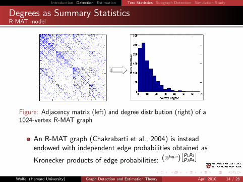
Degrees as Summary StatisticsR-MAT model

Figure: Adjacency matrix (left) and degree distribution (right) of a1024-vertex R-MAT graph

An R-MAT graph (Chakrabarti et al., 2004) is insteadendowed with independent edge probabilities obtained as

Kronecker products of edge probabilities: (⊗log n)[p1p3

p2p4

]Wolfe (Harvard University) Graph Detection and Estimation Theory April 2010 14 / 26


Detecting Embedded SubgraphsA question of p-values

Figure: Clique (left) and background R-MAT graph (right) combine toyield a detection task

Locating (with high probability) an embedded clique in givenrandom graph relies on its low likelihood under thebackground model

It is nontrivial to detect such embeddings directly via theempirical degree distribution



Algorithmic ApproachSubgraph detection via the modularity matrix

We may observe theembedding of verticesinduced by the first twoprincipal eigenvectors of themodularity matrix

A Chi-squared test on theexpected proportion ofvertices embedded into eachof the 4 quadrants yieldsgood performance

Maximizing over rotationangle in the plane canfurther improve test power

Figure: Without (top) & with (bottom) embedding



Brief Simulation StudyDetection results across various subgraph densities

0 0.2 0.4 0.6 0.8 1

0

0.2

0.4

0.6

0.8

1

ROC: R−MAT Background

Probability of False Alarm

Pro

babi

lity

of D

etec

tion

70%75%

80%

85%

90%

95%100%

0 50 100 150 200 250 300 3500

50

100

150

200

250

300

350

400

450

500

χ2max

Sam

ple

Pro

port

ion

R−MAT w/ Embedding: Distribution of Test Statistics

Background AloneBackground and Foreground

Operating characteristics of the subgraph detection test,shown for various subgraph densities (left), with empiricalsampling distributions of the test statistic shown for the caseof a 12-vertex clique (right)


Introduction Detection Estimation Point Process Estimation Data Analysis







A Point Process Model for GraphsLikelihood-based formulation

In many applications, a data matrix X comes in the form ofcounts with associated time stamps: for example, pairwisee-mail exchanges, text messages, or phone conversations

Here, given a set of individuals labeled 1, 2, . . . , n underobservation for times t ∈ (0,T ], we choose to model theinteractions between individuals i and j as a point process

ξij(t) = #{s ∈ (0, t] : node i interacts with node j at time s}

For s < t we set ξij(s, t] ≡ ξij(t)− ξij(s) to be the number oftimes that i and j interact in (s, t], and we assume theinteractions to be instantaneous and dyadically independent



A Point Process Model for GraphsLikelihood-based formulation

Under mild assumptions, the intensity

λij(t) ≡ limδ→0

E [ξij(t + δ)− ξij(t)]

δ

exists at all times t ∈ (0,T ]

Independence of interactions in non-overlapping intervalsresults in ξij(s, t] being a Poisson random variable. We referto its rate parameter simply by λij

The total number of counts Xij ≡ ξij(T ) in a given interval isthus a sufficient statistic for λij , and elements of the datamatrix X are independent with

P(Xij = xij) =(λijT )xij

xij !e−λijT



A Log-Linear Model for IntensitiesRelated to the gravity model and network traffic analysis

In this modeling context, the adjacency matrix A is simply aright-censored version of the data matrix X

Under our assumptions, then, Aij is a Bernoulli randomvariable with

P(Aij = 1) = 1− e−λijT

A simple log-linear model is given by

log λij = η + αi + αj , i 6= j

with the identifiability constraint that∑

i αi = 0

In general, it is possible to prove consistency and asymptoticnormality of ML estimators for this model as T →∞, andderive the explicit form of the Fisher information



Maximum-Likelihood InferenceClosed-form solution and a connection to Chung-Lu

If self-loops are allowed, then maximum-likelihood estimatesare obtainable in closed form, via the standard exponentialfamily parameterization for a Poisson mean

In fact, such estimates are easily seen to be

λij =1

T

kikj∑i ′ ki ′

,

showing the relation to our earlier Chung-Lu model!

A simple Taylor argument shows that as long as λij is small,then the corresponding adjacency matrix has

P(Aij = 1) ≈kikj∑i ′ ki ′



Maximum-Likelihood InferenceStructural zeros

Asymptotic results are also available for fixed T , with n→∞

So-called structural zeros (as they arise in contingency tableanalysis) complicate matters—for instance, the prohibition ofself-loops

We can estimate such zeros directly from the observed graphdata—or, they may come directly from the application context

These typically preclude a closed-form MLE, but our earliermethod of Chung-Lu fitting can be used to initialize a sparsesolver. We are currently building an R package for the generalcase of directed graph fitting



Enron E-mail DataPer-week e-mail volume

010

020

030

040

050

0

Week

Num

ber

of e

mai

ls

1999 2000 2001 2002

●●●●●●●●●●●●●●●●●●●●●●●●●●●●●●●●●●●●

●●●●●●●●●●●●

●●●●●●●

●●●●

●

●●●●●●●●●●●●●●●●●●●●

●●●●●●

●

●

●

●

●

●

●●

●

●●●

●●●

●

●●●●

●

●●

●

●

●

●

●●

●●●●●

●

●

●

●●●●●

●

●●

●

●

●

●

●

●●●

●

●

●

●

●●●

●

●

●

●

●

●

●●

●

●

●●

●●

●●

●

●

●

●●

●

●

●

●

●

●●●●●

●●●●●●●●●●●●

2001−04−01

● ●

●

● ●● ●

●

●●

●

●

●

●

● ●

●● ●

●●

●

●

●

● ● ●●

●

●

● ●

●

●

Figure: E-mail volume per week from the Enron corpus (left) and asuitably time-homogeneous period (right)

The Enron e-mail corpus comprises 189 weeks of e-mailexchanges amongst 156 employees



Estimated ParametersPoint process model fitted to the Enron corpus

●●● ●●●●●●●●●●●●●●●●●●●●●●●●●●●●●●●●●●●●●●●●●●●●●●●●●●●●●●●●●●●●●●●●●●●●●●●●●●●●●●●●●●●●●●●●● ● ●● ●

Estimated send parameter

qalp

ha

−2 −1 0 1 2 3

−2

2N

orm

al q

uant

ile●●●●●●●●●●●●●●●●●●●●●●●●●●●●●●●●●●●●●●●●●●●●●●●●●●●●●●●●●●●●●●●●●●●●●●●●●●●●●●●●●●●●●●●●●●●●●●●●●●●●●●●●●●●●●●●●●●●●●●●●●●●●●●●●●

●

qbeta

Est

imat

ed r

ecei

ve p

aram

eter

−1

01

2

−2Normal quantile

●

●

●

●

●

● ●●

●

●

●

●● ●●

●

●

●

●

●

●●

●

●

●

●

●

●

●

●

●

●●

●

●

●

●

●

●

●

●

●

●

●●

●

●

●

●

●

●●●

●●

●

●

●

●

●

●

●

●●

●

● ●●

●

●

●

●

●

●

●

●

●

●

●

●

●

●●

●

●

●

●

●

●

●

●

●

●

●

●

●

●

●

●●●●●

●

●

●●●

●

●

●

●

●●

●

●

●

●

●●

●

●

●

●

●

●

●

●

●

●

●

●

●

●

●

●

●

●

●●

●

●●●

●●●●

●

●

●

●●

●

●

●

alpha

beta

Figure: Estimated parameters forthe Enron corpus

Estimate θ = (η, α, β) viamaximum likelihood, using 90identifiability constraints on2 · 156 + 1 = 313 parameters,giving 313− 90 = 223 d.o.f.

For an arbitrary node, i , thereis no apparent relationshipbetween the estimated sendparameter, αi , and receiveparameter, βi .

In this modeling framework, itis also possible to includecovariates (for instance,employee organizationalhierarchy)



SummaryGraph detection and estimation theory




MIT Lincoln Laboratory, NSF-DMS/MSBS/CISE, DARPA, and ARO

PECASE support is gratefully acknowledged


Date post:	04-Jun-2018
Category:	Documents
Upload:	ngohanh
View:	230 times
Download:	0 times

Graph Detection and Estimation Theory - (and algorithms ... · IntroductionDetectionEstimation...

Documents