Page 1
Basic Graph Theory
with Applications to Economics
Debasis Mishra∗
February 23, 2011
1 What is a Graph?
Let N = 1, . . . , n be a finite set. Let E be a collection of ordered or unordered pairs of
distinct 1 elements from N . A graph G is defined by (N, E). The elements of N are called
vertices of graph G. The elements of E are called edges of graph G. If E consists of
ordered pairs of vertices, then the graph is called a directed graph (digraph). When we
say graph, we refer to undirected graph, i.e., E consists of unordered pairs of vertices. To
avoid confusion, we write an edge in an undirected graph as i, j and an edge in a directed
graph as (i, j).
Figure 1 gives three examples of graphs. The rightmost graph in the figure is a di-
rected graph. In all the graphs N = 1, 2, 3, 4. In the leftmost graph in Figure 1, E =
1, 2, 2, 3, 2, 4, 3, 4. In the directed graph, E = (1, 2), (1, 3), (2, 3), (3, 2), (3, 4), (4, 1).
1 2
34
1 2
34
1 2
34
Figure 1: Examples of graph
∗Planning Unit, Indian Statistical Institute, 7 Shahid Jit Singh Marg, New Delhi 110016, India, E-mail:
[email protected]
1In standard graph theory, we do not require this distinct restriction.
1
Page 2
Often, we associate weights to edges of the graph or digraph. These weights can represent
capacity, length, cost etc. of an edge. Formally, a weight is a mapping from set of edges to
real numbers, w : E → R. Notice that weight of an edge can be zero or negative also. We
will learn of some economic applications where this makes sense. If a weight system is given
for a (di)graph, then we write (N, E, w) as the (di)graph.
1.1 Modeling Using Graphs: Examples
Example 1: Housing/Job Market
Consider a market of houses (or jobs). Let there be H = a, b, c, d houses on a street.
Suppose B = 1, 2, 3, 4 be the set of potential buyers, each of whom want to buy exactly
one house. Every buyer i ∈ B is interested in ∅ 6= Hi ⊆ H set of houses. This situation can
be modeled using a graph.
Consider a graph with the following set of vertices: N = H ∪ B (note that H ∩ B = ∅).
The only edges of the graph are of the following form: for every i ∈ B and every j ∈ Hi,
there is an edge between i and j. Graphs of this kind are called bipartite graphs, i.e., a
graph whose vertex set can be partitioned into two non-empty sets and the edges are only
between vertices which lie in separate parts of the partition.
Figure 2 is a bipartite graph of this example. Here, H1 = a, H2 = a, c, H3 =
b, d, H4 = c. Is it possible to allocate a unique house to every buyer?
1
2
3
4
a
b
c
d
Figure 2: A bipartite graph
If every buyer associates a value for every house, then it can be used as a weight of the
graph. Formally, if there is an edge (i, j) then w(i, j) denotes the value of buyer i ∈ B for
house j ∈ Hi.
2
Page 3
Example 2: Coauthor/Social Networking Model
Consider a model with researchers (or agents in Facebook site). Each researcher wants
to collaborate with some set of other researchers. But a collaboration is made only if both
agents (researchers) put substantial effort. The effort level of agent i for edge (i, j) is given
by w(i, j). This situation can be modeled as a directed graph with weight of edge (i, j) being
w(i, j).
Example 3: Transportation Networks
Consider a reservoir located in a state. The water from the reservoir needs to be supplied
to various cities. It can be supplied directly from the reservoir or via another cities. The
cost of supplying water from city i to city j is given and so is the cost of supplying directly
from reservoir to a city. What is the best way to connect the cities to the reservoir?
The situation can be modeled using directed or undirected graphs, depending on whether
the cost matrix is asymmetric or symmetric. The set of nodes in the graph is the set of cities
and the reservoir. The set of edges is the set of edges from reservoir to the cities and all
possible edges between cities. The edges can be directed or undirected. For example, if the
cities are located at different altitudes, then cost of transporting from i to j may be different
from that from j to i, in which case we model it as a directed graph, else as an undirected
graph.
2 Definitions of (Undirected) Graphs
If i, j ∈ E, then i and j are called end points of this edge. The degree of a vertex is
the number of edges for which that vertex is an end point. So, for every i ∈ N , we have
deg(i) = #j ∈ N : i, j ∈ E. In Figure 1, degree of vertex 2 is 3. Here is a simple lemma
about degree of a vertex.
Lemma 1 The number of vertices of odd degree is even.
Proof : Let O be the set of vertices of odd degree. Notice that if we take the sum of the
degrees of all vertices, we will count the number of edges exactly twice. Hence,∑
i∈N deg(i) =
2#E. Now,∑
i∈N deg(i) =∑
i∈O deg(i) +∑
i∈N\O deg(i). Hence, we can write,
∑
i∈O
deg(i) = 2#E −∑
i∈N\O
deg(i).
Now, right side of the above equation is even. This is because 2#E is even and for every
i ∈ N \O, deg(i) is even by definition. Hence, left side of the above equation∑
i∈O deg(i) is
even. But for every i ∈ O, deg(i) is odd by definition. Hence, #O must be even.
3
Page 4
A path is a sequence of distinct vertices (i1, . . . , ik) such that ij, ij+1 ∈ E for all
1 ≤ j < k. The path (i1, . . . , ik) is called a path from i1 to ik. A graph is connected if there
is a path between every pair of vertices. The middle graph in Figure 1 is not connected.
A cycle is a sequence of vertices (i1, . . . , ik, ik+1) with k > 2 such that ij, ij+1 ∈ E for
all 1 ≤ j ≤ k, (i1, . . . , ik) is a path, and i1 = ik+1. In the leftmost graph in Figure 1, a path
is (1, 2, 3) and a cycle is (2, 3, 4, 2).
A graph G′ = (N ′, E ′) is a subgraph of graph G = (N, E) if ∅ 6= N ′ ⊆ N , E ′ ⊆ E, and
for every i, j ∈ E ′ we have i, j ∈ N ′. A connected acyclic (that does not contain a cycle)
graph is called a tree. Graphs in Figure 1 are not trees, but the second and third graph
in Figure 3 are trees. A graph may contain several trees (i.e. connected acyclic subgraphs).
The spanning tree of a connected graph is a subgraph (N, E ′) such that (N, E ′) is a tree.
Note that E ′ ⊆ E and a spanning tree does not contain a cycle. By definition, every tree
(N ′, E ′) is a spanning tree of graph (N ′, E ′).
Figure 3 shows a connected graph (which is not a tree) and two of its spanning trees.
1
2 3
4
1
2 3
4
1
2 3
4
Figure 3: Spanning trees of a graph
2.1 Properties of Trees and Spanning Trees
We now prove some properties of trees and spanning trees.
Proposition 1 Every tree G′ = (N ′, E ′), where G′ is a subgraph of a graph G = (N, E),
satisfies the following properties.
1. There is a unique path from i to j in G′ for every i, j ∈ N ′.
2. If there is an edge i, j ∈ E \ E ′ with i, j ∈ N ′, adding i, j to E ′ creates a cycle.
3. By removing an edge from E ′ disconnects the tree.
4. Every tree with at least two vertices has at least two vertices of degree one.
5. #E ′ = #N ′ − 1.
4
Page 5
Proof :
1. Suppose there are at least two paths from i to j. Let these two paths be P1 =
(i, i1, . . . , ik, j) and P2 = (i, j1, . . . , jq, j). Then, consider the following sequence of
vertices: (i, i1, . . . , ik, j, jq, . . . , j1, i). This sequence of vertices is a cycle or contains a
cycle if both paths share edges, contradicting the fact that G′ is a tree.
2. Consider an edge i, j ∈ E \ E ′. In graph G′, there was a unique path from i to j.
The edge i, j introduces another path. This means the graph G′′ = (N ′, E ′ ∪ i, j)
is not a tree (from the claim above). Since G′′ is connected, it must contain a cycle.
3. Let i, j ∈ E ′ be the edge removed from G′. By the first claim, there is a unique path
from i to j in G′. Since there is an edge between i and j, this unique path is the edge
i, j. This means by removing this edge we do not have a path from i to j, and hence
the graph is no more connected.
4. We do this using induction on number of vertices. If there are two vertices, the claim
is obvious. Consider a tree with n vertices. Suppose the claim is true for any tree
with < n vertices. Now, consider any edge i, j in the tree. By (1), the unique path
between i and j is this edge i, j. Now, remove this edge from the tree. By (3), we
disconnect the tree into trees which has smaller number of vertices. Each of these trees
have either a single vertex or have two vertices with degree one (by induction). By
connecting edge i, j, we can increase the degree of one of the vertices in each of these
trees. Hence, there is at least two vertices with degree one in the original graph.
5. For #N ′ = 2, it is obvious. Suppose the claim holds for every #N ′ = m. Now, consider
a tree with (m + 1) vertices. By the previous claim, there is a vertex i that has degree
1. Let the edge for which i is an endpoint be i, j. By removing i, we get another
tree of subgraph (N ′ \ i, E ′ \ i, j). By induction, number of edges of this tree is
m − 1. Since, we have removed one edge from the original tree, the number of edges
in the original tree (of a graph with (m + 1) vertices) is m.
We prove two more important, but straightforward, lemmas.
Lemma 2 Let G = (N, E) be a graph and G′ = (N, E ′) be a subgraph of G such that
#E ′ = #N − 1. If G′ has no cycles then it is a spanning tree.
Proof : Call a subgraph of a graph G a component of G if it is maximally conntected, i.e.,
G′′ = (N ′′, E ′′) is a component of G = (N, E) if G′′ is connected and there does not exist
vertices i ∈ N ′′ and j ∈ N \N ′′ such that i, j ∈ E.
5
Page 6
Clearly, any graph can be partitioned into its components with a connected graph having
one component, which is the same graph. Now, consider a cycle-free graph G′ = (N, E ′) and
let G1, . . . , Gq be the components of G′ with number of vertices in component Gj being nj
for 1 ≤ j ≤ q. Since every component in a cycle-free graph is a tree, by Proposition 1 the
number of edges in component Gj is nj − 1 for 1 ≤ j ≤ q. Since the components have no
vertices and edges in common, the total number of edges in components G1, . . . , Gq is
(n1 − 1) + . . . + (nq − 1) = (n1 + n2 + . . . + nq)− q = #N − q.
By our assumption in the claim, the number of edges in G′ is #N − 1. Hence, q = 1, i.e.,
the graph G′ is a component, and hence a spanning tree.
Lemma 3 Let G = (N, E) be a graph and G′ = (N, E ′) be a subgraph of G such that
#E ′ = #N − 1. If G′ is connected, then it is a spanning tree.
Proof : We show that G′ has no cycles, and this will show that G′ is a spanning tree. We
do the proof by induction on #N . The claim holds for #N = 2 and #N = 3 trivially.
Consider #N = n > 3. Suppose the claim holds for all graphs with #N < n. In graph
G′ = (N, E ′), there must be a vertex with degree 1. Else, every vertex has degree at least two
(it cannot have degree zero since it is connected). In that case, the total degree of all vertices
is 2#E ≥ 2n or #E = n−1 ≥ n, which is a contradiction. Let this vertex be i and let i, j
be the unique edge for which i is an endpoint. Consider the graph G′′ = (N\i, E ′\i, j).
Clearly, G′′ is connected and number of edges in G′′ is one less than n− 1, which equals the
number of edges in E ′ \ i, j. By our induction hypothesis, G′′ has no cycles. Hence, G′
cannot have any cycle.
3 The Minimum Cost Spanning Tree Problem
Consider a graph G = (N, E, w), i.e., a weighted graph. Assume G to be connected. Imagine
the weights to be costs of traversing an edge. So, w ∈ R#E+ . The minimum cost spanning
tree (MCST) problem is to find a spanning tree of minimum cost in graph G. Figure 4
shows a weighted graph. In this figure, one can imagine one of the vertices as “source” (of
water) and other vertices to be cities. The weights on edges may represent cost of supplying
water from one city to another. In that case, the MCST problem is to find a minimum cost
arrangement (spanning tree) to supply water to cities.
There are many greedy algorithms that find an MCST. We give a generic algorithm, and
show one specific algorithm that falls in this generic class.
The generic greedy algorithm grows an MCST one edge at a time. The algorithm manages
a subset A of edges that is always a subset of some MCST. At each step of the algorithm, an
6
Page 7
b
cd 4
3
2
2
1
1
a
Figure 4: The minimum cost spanning tree problem
edge i, j is added to A such that A ∪ i, j is a subset of some MCST. We call such an
edge a safe edge for A (since it can be safely added to A without destroying the invariant).
In Figure 4, A can be taken to be b, d, a, d, which is a subset of an MCST. A safe edge
for A is a, c.
Here is the formal procedure:
1. Set A = ∅.
2. If (N, A) is not a spanning tree, then find an edge i, j that is safe for A. Set
A← A ∪ i, j and repeat from Step 2.
3. If (N, A) is a spanning tree, then return (N, A).
Remark: After Step 1, the invariant (that in every step we maintain a set of edges which
belong to some MCST) is trivially satisfied. Also, if A is not a spanning tree but a subset of
an MCST, then there must exist an edge which is safe.
The question is how to identify safe edges. We discuss one such rule. The algorithm we
discuss is due to Kruskal, and hence called the Kruskal’s algorithm. For this, we provide
some definitions. A cut in a graph G = (N, E) is a partition of set of vertices (V, N \ V )
with V 6= N and V 6= ∅. An edge i, j crosses a cut (V, N \V ) if i ∈ V and j ∈ N \V . We
say a cut (V, N \ V ) respects a set of edges A if no edge from A crosses the cut. A light
edge crossing a cut (V, N \ V ) is an edge that has the minimum weight among all the edges
crossing the cut (V, N \ V ).
Figure 5 shows a graph and two of its cuts. The first cut is (1, 2, 3, 4, 5, 6). The
following set of edges respect this cut 1, 2, 1, 3. Also, the set of edges 4, 5, 5, 6
and the set of edges 1, 3, 4, 5 respect this cut. Edges 1, 4, 2, 6, 3, 4 cross this
cut.
The following theorem says how a light edge of an appropriate cut is a safe edge.
7
Page 8
5
14
5
62
3
6
3
4
2
1
Figure 5: Cuts in a graph
Theorem 1 Let G = (N, E, w) be a connected graph. Let A ⊂ T ⊆ E be a subset of edges
such that (N, T ) is an MCST of G. Let (V, N \ V ) be any cut of G that respects A and let
i, j be a light edge crossing (V, N \ V ). Then edge i, j is a safe edge for A.
Proof : Let A be a subset of edges of MCST (N, T ). If i, j ∈ T , then we are done. So, we
consider the case when i, j /∈ T . Since (N, T ) is a spanning tree, adding edge i, j to T
creates a cycle (Proposition 1). Hence, the sequence of vertices in the set of edges T ∪i, j
contains a cycle between vertex i and j - the unique cycle it creates consists of the unique
path from i to j in MCST (N, T ) and the edge i, j. This cycle must cross the cut (V, N \V )
at least twice - once at i, j and the other at some edge a, b 6= i, j such that a ∈ V ,
b ∈ N \ V which crosses the cut (V, N \ V ). Note that a, b ∈ T . If we remove edge a, b,
then this cycle is broken and we have no cycle in the graph G′′ = (N, (T ∪i, j)\a, b).
By Proposition 1, there are #N − 1 edges in (N, T ). Hence, G′′ also has #N − 1 edges. By
Lemma 2, G′′ is a spanning tree.
Let T ′ = (T∪i, j)\a, b. Now, the difference of edge weights of T and T ′ is equal to
w(a, b)−w(i, j). Since (N, T ) is an MCST, we know that w(a, b)−w(i, j) ≤ 0. Since
i, j is a light edge of cut (V, N\V ) and a, b crosses this cut, we have w(a, b) ≥ w(i, j).
Hence, w(a, b) = w(i, j). Hence (N, T ′) is an MCST.
This proves that (A ∪ i, j) ⊆ T ′. Hence, i, j is safe for A.
The above theorem almost suggests an algorithm to compute an MCST. Consider the
following algorithm. Denote by V (A) the set of vertices which are endpoints of edges in A.
1. Set A = ∅.
2. Choose any vertex i ∈ N and consider the cut (i, N \ i). Let i, j be a light edge
of this cut. Then set A← A ∪ i, j.
3. If A contains #N − 1 edges then return A and stop. Else, go to Step 4.
8
Page 9
4. Consider the cut (V (A), N \ V (A)). Let i, j be a light edge of this cut.
5. Set A← A ∪ i, j and repeat from Step 3.
This algorithm produces an MCST. To see this, by Theorem 1, in every step of the
algorithm, we add an edge which is safe. This means the output of the algorithm contains
#N − 1 edges and no cycles. By Lemma 2, this is a spanning tree. By Theorem 1, this is
an MCST.
We apply this algorithm to the example in Figure 4. In the first iteration of the algorithm,
we choose vertex a and consider the cut (a, b, c, d). A light edge of this cut is a, c. So,
we set A = a, c. Then, we consider the cut (a, c, b, d). A light edge of this cut is
a, d. Now, we set A = a, c, a, d. Then, we consider the cut (a, c, d, b). A light
edge of this cut is b, d. Since (N, a, c, a, d, b, d) is a spanning tree, we stop. The
total weight of this spanning tree is 1 + 2 + 1 = 4, which gives the minimum weight over all
spanning trees. Hence, it is an MCST.
4 Application: The Minimum Cost Spanning Tree Game
In this section, we define a coopearative game corresponding to the MCST problem. To do
so, we first define the notion of a cooperative game and a well known stability condition for
such games.
4.1 Cooperative Games
Let N be the set of agents. A subset S ⊆ N of agents is called a coalition. Let Ω be the set
of all coalitions. A cooperative game is a tuple (N, c) where N is a finite set of agents and
c is a characteristic function defined over set of coalitions Ω, i.e., c : Ω → R. The number
c(S) can be thought to be the cost incurred by coalition S when they cooperate 2.
The problem is to divide the total cost c(N) amongst the agents in N when they coop-
erate. We give an example of a cooperative game and analyze it below. Before that, we
describe a well known solution concept of core.
A cost vector x assigns every player a cost in a game (N, c). The core of a cooperative
game (N, c) is the set of cost vectors which satisfies a stability condition.
Core(N, c) = x ∈ R#N :∑
i∈N
xi = c(N),∑
i∈S
xi ≤ c(S) ∀ S ( N
2Cooperative games can be defined with value functions also, in which case notations will change, but
ideas remain the same.
9
Page 10
2
34
1 2
1
1
23
0
Figure 6: An MCST game
Every cost vector in the core is such that it distributes the total cost c(N) amongst agents
in N and no coalition of agents can be better off by forming their independent coalition.
There can be many cost vectors in a core or there may be none. For example, look at
the following game with N = 1, 2. Let c(12) = 5 and c(1) = c(2) = 2. Core conditions
tell us x1 ≤ 2 and x2 ≤ 2 but x1 + x2 = 5. But there are certain class of games which have
non-empty core (more on this later). We discuss one such game.
4.2 The Minimum Cost Spanning Tree Game
The minimum cost spanning tree game (MCST game) is defined by set of agents N =
1, . . . , n and a source agent to whom all the agents in N need to be connected. The
underlying graph is (N ∪ 0, E, c) where E = i, j : i, j ∈ N ∪ 0, i 6= j and c(i, j)
denotes the cost of edge i, j. For any S ⊆ N , let S+ = S ∪ 0. When a coalition of
agents S connect to source, they form an MCST using edges between themseleves. Let c(S)
be the total cost of an MCST when agents in S form an MCST with the source. Thus, (N, c)
defines a cooperative game.
An example is given in Figure 6. Here N = 1, 2, 3 and c(123) = 4, c(12) = 4, c(13) =
3, c(23) = 4, c(1) = 2, c(2) = 3, c(3) = 4. It can be verified that x1 = 2, x2 = 1 = x3 is in the
core. The next theorem shows that this is always the case.
For any MCST (N, T ), let p(i), i be the last edge in the unique path from 0 to agent i.
Define xi = c(p(i), i) for all i ∈ N . Call this the Bird allocation - named after the inventor
of this allocation.
Figure 7 gives an example with 5 agents (the edges not show have very high cost). The
MCST is shown with red edges in Figure 7. To compute Bird allocation of agent 1, we
observe that the last edge in the unique path from 0 to 1 in the MCST is 0, 1, which has
cost 5. Hence, cost allocation of agent 1 is 5. Consider agent 2 now. The unique path from
0 to 2 in the MCST has edges, 0, 3 followed by 3, 2. Hence, the last edge in this path
10
Page 11
45
6
38
63
4
8
7
0
1
2
3
4
5
Figure 7: Bird allocation
0
12
1
22
Figure 8: More than one Bird allocation
is 3, 2, which has a cost of 3. Hence, cost allocation of agent 2 is 3. Similarly, we can
compute cost allocations of agents 3,4, and 5 as 4, 6, and 3 respectively.
There may be more than one Bird allocation. Figure 8 illustrates that. There are two
MCSTs in Figure 8 - one involving edges 0, 1 and 1, 2 and the other involving edges
0, 2 and 1, 2. The Bird allocation corresponding to the first MCST is: agent 1’s cost
allocation is 2 and that of agent 2 is 1. The Bird allocation corresponding to the second
MCST is: agent 2’s cost allocation is 2 and that of agent 1 is 2.
Theorem 2 Any Bird allocation is in the core of the MCST game.
Proof : For any Bird allocation x, by definition∑
i∈N xi = c(N). Consider any coalition
S ( N . Assume for contradiction c(S) <∑
i∈S xi.
11
Page 12
Let (N, T ) be an MCST for which the Bird allocation x is defined. Delete for every i ∈ S,
the edge ei = p(i), i (last edge in the unique path from 0 to i) from the MCST (N, T ).
Let this new graph be (N, T ). Then, consider the MCST corresponding to nodes S+ (which
only use edges having endpoints in S+). Such an MCST has #S edges by Proposition 1.
Add the edges of this tree to (N, T ). Let this graph be (N, T ′). Note that (N, T ′) has the
same number (#N − 1) edges as the MCST (N, T ). We show that (N, T ′) is connected. It
is enough to show that there is a path from source 0 to every vertex i ∈ N . We consider two
cases.
Case 1: Consider any vertex i ∈ S. We have a path from 0 to i in (N, T ′) by the MCST
corresponding S+.
Case 2: Consider any vertex i /∈ S. Consider the path in (N, T ) from 0 to i. Let k be the
last vertex in this path such that k ∈ S. So, all the vertices from k to i are not in S in the
path from 0 to i. If no such k exists, then the path from 0 to i still exists in (N, T ′). Else,
we know from Case 1, there is a path from 0 to k in (N, T ′). Take this path and go along
the path from k to i in (N, T ). This defines a path from 0 to i in (N, T ′).
This shows that (N, T ′) is connected and has #N − 1 edges. By Lemma 3, (N, T ′) is a
spanning tree.
Now, the new spanning tree has cost c(N)−∑
i∈S xi + c(S) < c(N) by assumption. This
violates the fact that the original tree is an MCST.
If there are more than one Bird allocations, each of them belongs to the core. Moreover,
any convex combination of these Bird allocations is also in the core (this is easy to verify,
and left as an exercise).
5 Hall’s Marriage Theorem
Consider an economy with a finite set of houses H and a finite set of buyers B with #B ≤
#H . We want to find if houses and buyers can matched in a compatible manner. For every
buyer i ∈ B, a set of houses ∅ 6= Hi are compatible. Every buyer wants only one house from
his compatible set of houses. We say buyer i likes house j if and only if j ∈ Hi. This can be
represented as a bipartite graph with vertex set H ∪B and edge set E = i, j : i ∈ B, j ∈
Hi. We will denote such a bipartite graph as G = (H ∪ B, Hii∈B).
We say two edges i, j, i′, j′ in a graph are disjoint if i, j, i′, j′ are all distinct, i.e.,
the endpoints of the edges are distinct. A set of edges are disjoint if every pair of edges in
that set are disjoint. A matching in graph G is a set of edges which are disjoint. We ask
whether there exists a matching with #B edges, i.e., where all the buyers are matched.
12
Page 13
Figure 9 shows a bipartite graph with a matching: 1, b, 2, a, 3, d, 4, c.
1
2
3
4
a
b
c
d
Figure 9: A bipartite graph with a matching
Clearly, a matching where all buyers are matched will not always exist. Consider the case
where #B ≥ 2 and for every i ∈ B, we have Hi = j for some j ∈ H , i.e, every buyer likes
the same house - j. No matching where all the buyers are matched is possible in this case.
In general, if we take a subset S ⊆ B of buyers and take the set of houses that buyers in
S like: D(S) = ∪i∈SHi, then #S ≤ #D(S) is necessary for a matching where all buyers are
matched to exist. Else, number of houses who buyers in S like are less, and so some buyer
cannot be matched. For example, if we pick a set of 5 buyers who like only a set of 3 houses,
then we cannot match some buyers.
Hall’s marriage theorem states that this condition is also sufficient.
Theorem 3 A matching with #B edges in a bipartite graph G = (H ∪ B, Hii∈B) exists
if and only if for every ∅ 6= S ⊆ B, we have #S ≤ #D(S), where D(S) = ∪i∈SHi.
Proof : Suppose a matching with #B edges exists in G. Then, we have #B disjoint edges.
Denote this set of edges as M . By definition, every edge in M has a unique buyer and a
unique house as endpoints, and for every i, j ∈ M we have j ∈ Hi. Now, for any set of
buyers ∅ 6= S ⊆ B, we define M(S) = j ∈ H : i, j ∈M, i ∈ S - the set of houses matched
to buyers in S in matching M . We know that #S = #M(S). By definition M(S) ⊆ D(S).
Hence #S ≤ #D(S).
Suppose for every ∅ 6= S ⊆ B, we have #S ≤ #D(S). We use induction to prove that
a matching with #B edges exists. If #B = 1, then we just match her to one of the houses
she likes (by our condition she must like at least one house). Suppose a matching with #B
edges exists for any graph with less than l + 1 buyers. We will show that a matching with
#B edges exists for any graph with #B = l + 1 buyers.
There are two cases to consider.
Case 1: Suppose #S < #D(S) for every ∅ 6= S ( L (notice proper subset). Then choose
an arbitrary buyer i ∈ B and any j ∈ Hi, and consider the edge i, j. Now consider
the bipartite graph G′ = (H \ j ∪ B \ i, Hk \ jk∈B\i). Now, G′ is a graph with
13
Page 14
l buyers. Since we have removed one house and one buyer from G to form G′ and since
#S ≤ #D(S)− 1 for all ∅ 6= S ( B, we will satisfy the condition in the theorem for graph
G′. By induction assumption, a matching exists in graph G′ with #B − 1 edges. This
matching along with edge i, j forms a matching of graph G with #B edges.
Case 2: For some ∅ 6= S ( B, we have #S = #D(S). By definition #S < #B, and hence
by induction we have a matching in the graph G′ = (S ∪ D(S), Hii∈S) with #S edges.
Now consider the graph G′′ = ((H \D(S)) ∪ (B \ S), Hi \D(S)i∈B\S). We will show that
the condition in the theorem holds in graph G′′.
Consider any ∅ 6= T ⊆ (B \ S). Define D′(T ) = D(T ) \ D(S). We have to show that
#T ≤ #D′(T ). We know that #(T ∪S) ≤ #D(T ∪S). We can write #D(T ∪S) = #D(S)+
#(D(T ) \D(S)) = #D(S) + #D′(T ). Hence, #(T ∪ S) = #T + #S ≤ #D(S) + #D′(T ).
But #S = #D(S). Hence, #T ≤ #D′(T ). Hence, the condition in the theorem holds for
graph G′′. By definition #(B \ S) < #B. So, we apply the induction assumption to find
a matching in G′′ with #(B \ S) edges. Clearly, the matchings of G′ and G′′ do not have
common edges, and they can be combined to get a matching of G with #B edges.
Remark: Hall’s marriage theorem tells you when a matching can exist in a bipartite graph.
It is silent on the problem of finding a matching when it exists. We will study other results
about existence and feasibility later.
6 Maximum Matching in Bipartite Graphs
We saw in the last section that matching all buyers in a bipartite matching problem requires
a combinatorial condition hold. In this section, we ask the question - what is the maximum
number of matchings that is possible in a bipartite graph? We will also discuss an algorithm
to compute such a maximum matching.
6.1 M-Augmenting Path
We start with the notion of augmenting path in an arbitrary undirected graphs. To remind,
in a graph G = (N, E), a matching M ⊆ E is a set of disjoint edges in G. Here, one can
think of nodes in G to be students, the set of edges to be set of possible pairings of students.
The problem of finding roommates for students can be thought to be a problem of finding a
matching (of maximum size) in G. Figures 10 and 11 show two matchings in a graph - dark
edges represent a matching.
Before we introduce the definition of an augmenting path, we introduce some terminology.
The length of a path (cycle) is the number of edges in a path (cycle). Given a graph
G = (N, E), a set of vertices S ⊆ N is covered by a set of edges X ⊆ E if every vertex
14
Page 15
1
23
4
56
Figure 10: A matching in a graph
1
23
4
56
Figure 11: A matching in a graph
in S is an endpoint of some edge in X. If (i1, i2, . . . , ik) is a path, then i1 and ik are called
endpoints of this path.
Definition 1 Let M be a matching in a graph G = (N, E). A path P (with non-zero
length) in G is called M-augmenting if its endpoints are not covered by M and its edges
are alternatingly in and out of M .
Note that an M-augmenting path need not contain all the edges in M . Suppose an
M-augmenting path contains k edges from E \ M . Note that k ≥ 1 as endpoints of an
M-augmenting path are not covered by M . Then, there are exactly k − 1 edges from M in
this path. If k = 1, then we have no edges from M in this path. So, an M-augmenting path
has odd (2k− 1) number of edges, and the number of edges in M is less than the number of
edges out of M in an M-augmenting path.
Figures 12 and 13 show two matchings and their respective M-augmenting paths.
Definition 2 A matching M in graph G = (N, E) is maximum if there does not exist
another matching M ′ in G such that #M ′ > #M .
It can be verified that the matching in Figure 10 is a maximum matching. There is
an obvious connection between maximum matchings and augmenting paths. For example,
15
Page 16
1
23
4
56
Figure 12: An M-augmenting path for a matching
1
23
4
56
Figure 13: An M-augmenting path for a matching
notice the maximum matching M in Figure 10. We cannot seem to find an M-augmenting
path for this matching. On the other hand, observe that the matching in Figure 11 is not
a maximum matching (the matching in Figure 10 has more edges), and Figure 12 shows an
augmenting path of this matching. This observation is formalized in the theorem below.
Theorem 4 Let G = (N, E) be a graph and M be a matching in G. The matching M is a
maximum matching if and only if there exists no M-augmenting paths.
Proof : Suppose M is a maximum matching. Assume for contradiction that P is an M-
augmenting path. Let EP be the set of edges in P . Now define, M ′ = (EP \M)∪ (M \EP ).
By definition of an augmenting path, EP \M contains more edges than EP ∩M . Hence, M ′
contains more edges than M . Also, by definition of an augmenting path, the edges in EP \M
are disjoint. Since M is a matching, the set of edges in (M \ EP ) are disjoint. Also, by the
definition of the augmenting path (ends of an augmenting path are not covered in M), we
have that the edges in (EP \M) and edges in (M \EP ) cannot share an endpoint. Hence, M ′
is a set of disjoint edges, i.e., a matching with size larger than M . This is a contradiction.
Now, suppose that there exists no M-augmenting path. Assume for contradiction that
M is not a maximum matching and there is another matching M ′ larger than M . Consider
the graph G′ = (N, M ∪M ′). Hence, every vertex of graph G′ has degree in 0, 1, 2. Now,
16
Page 17
partition G′ into components. Each component has to be either an isolated vertex or a path
or a cycle. Note that every cycle must contain equal number of edges from M and M ′. Since
the number of edges in M ′ is larger than that in M , there must exist a component of G′
which is a path and which contains more edges from M ′ than from M . Such a path forms
an M-augmenting path. This is a contradiction.
Theorem 4 suggests a simple algorithm for finding a maximum matching. The algorithm
starts from some arbitrary matching, may be the empty one. Then, it searches for an
augmenting path of this matching. If there is none, then we have found a maximum matching,
else the augmenting path gives us a matching larger than the current matching, and we
repeat. Hence, as long as we can find an augmenting path for a matching, we can find a
maximum matching.
6.2 Algorithm for Maximum Matching in Bipartite Graphs
We describe a simple algorithm to find a maximum matching in bipartite graphs. We have
already laid the foundation for such an algorithm earlier in Theorem 4, where we proved
that any matching is either a maximum matching or there exists an augmenting path of that
matching which gives a larger matching than the existing one. We use this fact.
The algorithm starts from an arbitrary matching and searches for an augmenting path of
that matching. Let M be any matching of bipartite graph G = (N, E) and N = B ∪L such
that for every i, j ∈ E we have i ∈ B and j ∈ L. Given the matching M , we construct a
directed graph GM from G as follows:
• The set of vertices of GM is N .
• For every i, j ∈M with i ∈ B and j ∈ L, we create the edge (i, j) in graph GM , i.e.,
edge from i to j.
• For every i, j /∈M with i ∈ B and j ∈ L, we create the edge (j, i) in graph GM , i.e.,
edge from j to i.
Consider the bipartite graph in Figure 14 (left one) and the matching M shown with dark
edges. For the matching M , the corresponding directed graph GM is shown on the right in
Figure 14.
Let BM be the set of vertices in B not covered by M and LM be the set of vertices in L
not covered by M . Note that every vertex in BM has no outgoing edge and every vertex in
LM has no incoming edge.
We first prove a useful lemma. For every directed path in GM the corresponding path in
G is the path obtained by removing the directions of the edges in the path of GM .
17
Page 18
1
2
3
4
a
b
c
d d
1
2
3
4
a
b
c
Figure 14: A bipartite graph with a matching
Lemma 4 A path in G is an M-augmenting path if and only if it is the corresponding path
of a directed path in GM which starts from a vertex in LM and ends at a vertex in BM .
Proof : Consider a directed path P in GM which starts from a vertex in LM and ends at
vertex in BM . By definition, the endpoints of P are not covered by M . Since edges from L
to B are not in M and edges from B to L are in M in GM , alternating edges in P is in and
out of M . Hence, the corresponding path in G is an M-augmenting path.
For the converse, consider an M-augmenting path in G and let P be this path in GM
with edges appropriately oriented. Note that endpoints of P are not covered by M . Hence,
the starting point of P is in LM and the end point of P is in BM - if the starting point
belonged to BM , then there will be no outgoing edge and if the end point belonged to LM ,
then there will be no incoming edge. This shows that P is a directed path in GM which
starts from a vertex in LM and ends at a vertex in BM .
Hence, to find an augmenting path of a matching, we need to find a specific type of path
in the corresponding directed graph. Consider the matching M shown in Figure 14 and the
directed graph GM . There is only one vertex in LM - b. The directed path (b, 1, a, 2, c, 4)
is a path in GM which starts at LM and ends at BM (see Figure 15). The corresponding
path in G gives an M-augmenting path. The new matching from this augmenting path
assigns: 1, b, 2, a, 4, c, 3, d (see Figure 15). It is now easy to see that this is indeed
a maximum matching (if it was not, then we would have continued in the algorithm to find
an augmenting path of this matching).
6.3 Minimum Vertex Cover and Maximum Matching
The size of a maximum matching in a graph is the number of edges in the maximum
matching. We define vertex cover now and show its relation to matching. In particular, we
show that the minimum vertex cover and the maximum matching of a bipartite graph have
the same size.
18
Page 19
1
2
3
4
a
b
c
d d
1
2
3
4
a
b
c
Figure 15: A bipartite graph with a matching
Definition 3 Given a graph G = (N, E), a set of vertices C ⊆ N is called a vertex cover
of G if every edge in E has at least one end point in C. Further, C is called a minimum
vertex cover of G if there does not exist another vertex cover C ′ of G such that #C ′ < #C.
Clearly, the set of all vertices in a graph consists of a vertex cover. But this may not be
a minimum vertex cover. We give some examples in Figure 16. Figure 16 shows two vertex
covers of the same graph - vertex covers are shown with black vertices. The first one is not
a minimum vertex cover but the second one is.
23
4
56
11
2 3
4
56
Figure 16: Vertex cover
An application of the vertex cover can be as follows. Suppose the graph represents a
city: the vertices are squares and the edges represent streets. The city plans to deploy
security office (or medical store or emergency service or park) at squares to monitor streets.
A security officer deployed at a square can monitor all streets which have an endpoint in
that square. The minimum vertex cover problem finds the minimum set of squares where
one needs to put a security officer to monitor all the streets.
Fix a graph G. Denote the size of maximum matching in G as ν(G) - this is also called
the matching number of G. Denote the size of minimum cover in G as τ(G) - this is also
called the vertex cover number of G.
Lemma 5 For any graph G, ν(G) ≤ τ(G).
19
Page 20
Proof : Any vertex cover contains at least one end point of every edge of a matching. Hence,
consider the maximum matching. A vertex cover will contain at least one vertex from every
edge of this matching. This implies that for every graph G, ν(G) ≤ τ(G).
Lemma 5 can hold with strict inequality in general graphs. Consider the graph in Figure
17. A minimum vertex cover, as shown with black vertices, has two vertices. A maximum
matching, as shown with the dashed edge, has one edge.
1
2 3
Figure 17: Matching number and vertex cover number
But the relationship in Lemma 5 is equality in case of bipartite graphs as the following
theorem, due to Konig shows.
Theorem 5 (Konig’s Theorem) Suppose G = (N, E) is a bipartite graph. Then, ν(G) =
τ(G).
1
2
3
4
a
b
c
d
Figure 18: Matching number and vertex cover number in bipartite graphs
Figure 18 shows a bipartite graph and its maximum matching edges (in dark) and mini-
mum vertex cover (in dark). For the bipartite graph in Figure 18 the matching number (and
the vertex cover number) is two.
20
Page 21
We will require the following useful result for proving Theorem 5. A graph may have
multiple maximum matchings. The following result says that there is at least one vertex
which is covered by every maximum matching if the graph is bipartite.
Lemma 6 Suppose G = (N, E) is a bipartite graph with E 6= ∅. Then, there exists a vertex
in G which is covered by every maximum matching.
Proof : Assume for contradiction that every vertex is not covered by some maximum match-
ing. Consider any edge i, j ∈ E. Suppose i is not covered by maximum matching M and
j is not covered by maximum matching M ′. Note that j must be covered by M - else adding
i, j to M gives another matching which is larger in size than M . Similarly, i must be
covered by M ′. Note that the edge i, j is not in (M ∪M ′).
Consider the graph G′ = (N, M ∪ M ′). A component of G′ must contain i (since M ′
covers i). Such a component will have alternating edges in and out of M and M ′. Since i
is covered by M ′ and not by M , i must be an end point in this component. Further, this
component must be a path - denote this path by P . Note that P contains alternating edges
from M and M ′ (not in M). The other endpoint of P must be a vertex k which is covered by
M - else, P defines an M-augmenting path, contradicting that M is a maximum matching
by Theorem 4. This also implies that k is not covered by M ′ and P has even number of
edges.
We argue that P does not contain j. Suppose P contains j. Since j is covered by M and
not by M ′, j must be an endpoint of P . Since G is bipartite, let N = B ∪L and every edge
u, v ∈ E is such that u ∈ B and v ∈ L. Suppose i ∈ B. Since the number of edges in P is
even, both the end points of P must be in B. This implies that j ∈ B. This contradicts the
fact that i, j is an edge in G.
So, we conclude that j is not in P . Consider the path P ′ formed by adding edge i, j
to P . This means j is an end point of P ′. Note that j is not covered by M ′ and the other
endpoint k of P ′ is also not covered by M ′. We have alternating edges in and out of M ′ in
P ′. Hence, P ′ defines an M ′-augmenting path. This is a contradiction by Theorem 4 since
M ′ is a maximum matching.
Proof of Theorem 5
Proof : We use induction on number of vertices in G. The theorem is clearly true if G has
one or two vertices. Suppose the theorem holds for any bipartite graph with less than n
vertices. Let G = (N, E) be a bipartite graph with n vertices. By Lemma 6, there must
exist a vertex i ∈ N such that every maximum matching of G must cover i. Let Ei be the
set of edges in G for which i is an endpoint. Consider the graph G′ = (N \i, E \Ei). Note
that G′ is bipartite and contains one less vertex. Hence, ν(G′) = τ(G′).
21
Page 22
We show that ν(G′) = ν(G) − 1. By deleting the edge covering i in any maximum
matching of G, we get a matching of G′. Hence, ν(G′) ≥ ν(G)−1. Suppose ν(G′) > ν(G)−1.
This means, ν(G′) ≥ ν(G). Hence, there exists a maximum matching of G′, which is also
a matching of G, and has as many edges as the maximum matching matching of G. Such
a maximum matching of G′ must be a maximum matching of G as well and cannot cover i
since i is not in G′. This is a contradiction since i is a vertex covered by every maximum
matching of G.
This shows that ν(G′) = τ(G′) = ν(G)− 1. Consider the minimum vertex cover C of G′
and add i to C. Clearly C ∪i is a vertex cover of G and has τ(G′)+1 vertices. Hence, the
minimum vertex cover of G must have no more than τ(G′) + 1 = ν(G) vertices. This means
τ(G) ≤ ν(G). But we know from Lemma 5 that τ(G) ≥ ν(G). Hence, τ(G) = ν(G).
Now, we show how to compute a minimum vertex cover from a maximum matching in a
bipartite graph. We leave the formal proof of the fact that this indeed produces a minimum
vertex cover as an exercise.
Consider the bipartite graph G in Figure 18. Figure 19 shows its maximum matching (in
dark edges) M and the directed graph GM suggested by Lemma 4. We first consider the set
of vertices reachable from the set of vertices in LM in GM - a vertex i is reachable from a
vertex j in a directed graph if there is a path from j to i. Call such a set of vertices RM . In
Figure 19, we have LM = c, d and RM = c, d, 1, b.
Define C := (L \RM) ∪ (B ∩RM).
We show that C defines a vertex cover of G. To see this, take any edge i, j where i ∈ B
and j ∈ L. If j ∈ L \ RM , then j ∈ C, and i, j is covered. If j ∈ RM , then there are
two cases: (1) i, j ∈M , in that case, the directed path to j must come from i, and hence
i ∈ RM ; (2) i, j /∈ M , then there is an edge from j to i in GM , and hence i ∈ RM . So,
j ∈ RM implies i ∈ RM , and hence i ∈ C.
Note that RM ∩ Bm = ∅ - because if some vertex in i ∈ RM belongs to BM , then it
must be the last vertex in the path which starts from a vertex in LM , and this will define an
M-augmenting path, a contradiction since M is a maximum matching.
Note that LM ⊆ RM . Hence, C is disjoint from LM . Since C is disjoint from BM , it is
disjoint from BM ∪ LM .
Further, no edge in M is contained in C. To see this, suppose i, j ∈ M and i, j ∈ C
with i ∈ B and j ∈ L. But this means i ∈ RM , which means j ∈ RM , which contradicts the
fact that j ∈ C.
The last two observations imply that #C ≤ #M . Therefore, C is a minimum vertex
cover. In Figure 19, we have C := 1, a, which is a minimum vertex cover.
22
Page 23
1
2
3
4
a
b
c
d
Figure 19: Minimum vertex cover from maximum matching
7 Basic Directed Graph Definitions
A directed graph is defined by a triple G = (N, E, w), where N = 1, . . . , n is the set
of n nodes, E ⊆ (i, j) : i, j ∈ N is the set of edges (ordered pairs of nodes), and w is a
vector of weights on edges with w(i, j) ∈ R denoting the weight or length of edge (i, j) ∈ E.
Notice that the length of an edge is not restricted to be non-negative. A complete graph is
a graph in which there is an edge between every pair of nodes.
a
b
c
d
e
f
5
4
10
−3
3
−2
2
1
4
Figure 20: A Directed Graph
A path is a sequence of distinct nodes (i1, . . . , ik) such that (ij , ij+1) ∈ E for all 1 ≤ j ≤
k−1. If (i1, . . . , ik) is a path, then we say that it is a path from i1 to ik. A graph is strongly
connected if there is a path from every node i ∈ N to every other node j ∈ N \ i.
A cycle is a sequence of nodes (i1, . . . , ik, ik+1) such that (i1, . . . , ik) is a path, (ik, ik+1) ∈
E, and i1 = ik+1. The length of a path or a cycle P = (i1, . . . , ik, ik+1) is the sum of the edge
lengths in the path or cycle, and is denoted as l(P ) = w(i1, i2) + . . . + w(ik, ik+1). Suppose
there is at least one path from node i to node j. Then, the shortest path from node i to
node j is a path from i to j having the minimum length over all paths from i to j. We denote
the length of the shortest path from i to j as s(i, j). We denote s(i, i) = 0 for all i ∈ N .
Figure 20 shows a directed graph. A path from a to f is (a, b, d, e, f). A cycle in the
graph is (c, d, e, c). The length of the path (a, b, d, e, f) is 5 + (−3) + (−2) + 4 = 4. The
23
Page 24
length of the cycle (c, d, e, c) is 1 + (−2) + 2 = 1. The possible paths from a to f with their
corresponding lengths are:
• (a, f): 10.
• (a, b, f): 5 + 3 = 8.
• (a, b, d, e, f): 5 + (−3) + (−2) + 4 = 4.
• (a, c, d, e, f): 4 + 1 + (−2) + 4 = 7.
Hence, s(a, f) = 4, and the shortest path from a to f is (a, b, d, e, f).
Here is a useful lemma.
Lemma 7 Suppose (i, i1, . . . , ik, j) is the shortest path from i to j in the digraph G =
(N, E, w). If G has no cycles of negative length, then for every ip ∈ i1, . . . , ik, s(i, ip) +
s(ip, j) = s(i, j).
Proof : Let P1 = (i, i1, . . . , ip) and P2 = (ip, . . . , ik, j). We show that l(P1) = s(i, ip) and
l(P2) = s(ip, j), and this will establish the claim.
By the definition of the shortest path, s(i, ip) ≤ l(P1). Assume for contradiction, s(i, ip) <
l(P1). This implies that there is some other path P3 from i to ip which is shorter than P1.
If P3 does not involve any vertex from P2, then P3 and P2 define a path from i to j, and
l(P3) + l(P2) < s(i, j). But this contradicts the fact that (i, i1, . . . , ik, j) is a shortest path.
If P3 involves a vertex from P2, then P3 and P2 will include cycles, which have non-negative
length. Removing these cycles from P2 and P3 will define a new path from i to j which has
shorter length. This is again a contradiction.
A similar argument works if s(ip, j) < l(P2).
7.1 Potentials
Definition 4 A potential of a directed graph G is a function p : N → R such that
p(j)− p(i) ≤ w(i, j) for all (i, j) ∈ E.
Figure 21 illustrates the idea of potentials.
Notice that if p is a potential of graph G, so is p(j) + αj∈N for all α ∈ R. Potentials
do not always exist. The following theorem provides a necessary and sufficient condition.
Theorem 6 There exists a potential of directed graph G = (N, E, w) if and only if G has
no cycles of negative length.
24
Page 25
i jw(i,j)
p(j)p(i)
p(i) + w(i,j) >= p(j)
Figure 21: Idea of potentials
Proof : Suppose a potential p exists of graph G. Consider a cycle (i1, . . . , ik, i1). By
definition of a cycle, (ij , ij+1) ∈ E for all 1 ≤ j ≤ k−1 and (ik, i1) ∈ E. Hence, we can write
p(i2)− p(i1) ≤ w(i1, i2)
p(i3)− p(i2) ≤ w(i2, i3)
. . . ≤ . . .
. . . ≤ . . .
p(ik)− p(ik−1) ≤ w(ik−1, ik)
p(i1)− p(ik) ≤ w(ik, i1).
Adding these inequalities, we get w(i1, i2)+. . .+w(ik−1, ik)+w(ik, i1) ≥ 0. The right had side
of the inequality is the length of the cycle (i1, . . . , ik, i1), which is shown to be non-negative.
Now, suppose every cycle in G has non-negative length. We construct another graph G′
from G as follows. The set of vertices of G′ is N ∪ 0, where 0 is a new (dummy) vertex.
The set of edges of G′ is E ∪ (0, j) : j ∈ N, i.e., G′ has all the edges of G and new edges
from 0 to every vertex in N . The weights of new edges in G′ are all zero, whereas weights
of edges in G remain unchanged in G′. Clearly, there is a path from 0 to every vertex in G′.
Observe that if G contains no cycle of negative length then G′ contains no cycle of negative
length. Figure 22 shows a directed graph and how the graph with the dummy vertex is
created.
1
2 3
45 −2
21
−3
4
1
4
2 −3 3
2
4−2
10
0
0 0
0
0
Figure 22: A directed graph and the new graph with the dummy vertex
25
Page 26
We claim that s(0, j) for all j ∈ N defines a potential of graph G. Consider any (i, j) ∈ E.
We consider two cases.
Case 1: The shortest path from 0 to i does not include vertex j. Now, by definition of
shortest path s(0, j) ≤ s(0, i) + w(i, j). Hence, s(0, j)− s(0, i) ≤ w(i, j).
Case 2: The shortest path from 0 to i includes vertex j. In that case, s(0, i) = s(0, j)+s(j, i)
(by Lemma 7). Hence, s(0, i)+w(i, j) = s(0, j)+s(j, i)+w(i, j). But the shortest path from
j to i and then edge (i, j) creates a cycle, whose length is given by s(j, i) + w(i, j). By our
assumption, s(j, i)+w(i, j) ≥ 0 (non-negative cycle length). Hence, s(0, i)+w(i, j) ≥ s(0, j)
or s(0, j)− s(0, i) ≤ w(i, j).
In both cases, we have shown that s(0, j)− s(0, i) ≤ w(i, j). Hence s(0, j) for all j ∈ N
defines a potential of graph G.
An alternate way to prove this part of the theorem is to construct G′ slightly differently.
Graph G′ still contains a new dummy vertex but new edges are now from vertices in G to
the dummy vertex 0. In such G′, there is a path from every vertex in N to 0. Moreover, G′
contains no cycle of negative length if G contains no cycle of negative length. We claim that
−s(j, 0) for all j ∈ N defines a potential for graph G. Consider any (i, j) ∈ E. We consider
two cases.
Case 1: The shortest path from j to 0 does not include vertex i. Now, by definition of
shortest path s(i, 0) ≤ w(i, j) + s(j, 0). Hence, −s(j, 0)− (−s(i, 0)) ≤ w(i, j).
Case 2: The shortest path from j to 0 includes vertex i. In that case, s(j, 0) = s(j, i)+s(i, 0).
Hence, s(j, 0) + w(i, j) = s(j, i) + w(i, j) + s(i, 0). But s(j, i) + w(i, j) is the length of
cycle created by taking the shortest path from j to i and then taking the direct edge (i, j).
By our assumption, s(j, i) + w(i, j) ≥ 0. Hence, s(j, 0) + w(i, j) ≥ s(i, 0), which gives
−s(j, 0)− (−s(i, 0)) ≤ w(i, j).
The proof of Theorem 6 shows a particular potential when it exists. It also shows an
elegant way of verifying when a system of inequalities (of the potential form) have a solution.
Consider the following system of inequalities. Inequalities of this form are called difference
26
Page 27
1 2
3
4
2
2−1
−3
0
1
Figure 23: A graphical representation of difference inequalities
inequalities.
x1 − x2 ≤ 2
x2 − x4 ≤ 2
x3 − x2 ≤ −1
x3 − x4 ≤ −3
x4 − x1 ≤ 0
x4 − x3 ≤ 1.
To find if the above system of inequalities have a solution or not, we construct a graph with
vertex set 1, 2, 3, 4 and an edge for every inequality with weights given by the right hand
side of the inequalities. Figure 23 shows the graphical representation. Clearly, a solution
to these difference inequalities correspond to potentials of this graph. It can be easily seen
that the cycle (3, 4, 3) in this graph has a length (−3) + 1 = (−2). Hence, there exists no
potential of this graph by Theorem 6.
From the proof of Theorem 6, we have established how to compute a potential when
it exists. It suggests that if we have a vertex from which a path exists to every vertex or
a vertex to which a path exists from every other vertex, then shortest such paths define a
potential.
Theorem 7 Suppose G = (N, E, w) is a directed graph with no cycle of negative length
and i is a vertex in G such that there is a path from i to every other vertex in G. Then
p(j) = s(i, j) for all j ∈ N \i and p(i) = 0 defines a potential of graph G. Similarly, if i is
a vertex in G such that there is a path from every other vertex in G to i, then p(j) = −s(j, i)
for all j ∈ N \ i and p(i) = 0 defines a potential of graph G.
27
Page 28
Proof : The proof is similar to the second part of proof of Theorem 6 - the only difference
being we do not need to construct the new graph G′ and work on graph G directly.
Figure 24 gives an example of a complete directed graph. It can be verified that this
graph does not have a cycle of negative length. Now, a set of potentials can be computed
using Theorem 7. For example, fix vertex 2. One can compute s(1, 2) = 3 and s(3, 2) = 4.
Hence, (−3, 0,−4) is a potential of this graph. One can also compute s(2, 1) = −2 and
s(2, 3) = −3, which gives (−2, 0,−3) to be another potential of this graph.
−2
−1
43
1
23
−3
4
Figure 24: Potentials for a complete directed graph
8 Unique Potentials
We saw that given a digraph G = (N, E, w), there may exist many potentials. Indeed, if p
is a potential, then so is q, where q(j) = p(j) + α for all j ∈ N and α ∈ R is some constant.
There are other ways to construct new potentials from a given pair of potentials. We say
a set of n-dimensional vectors X ⊆ Rn form a lattice if x, y ∈ X implies x ∧ y, defined by
(x ∧ y)i = min(xi, yi) for all i, and x ∨ y, defined by (x ∨ y)i = max(xi, yi) for all i both
belong to X. We give some examples of lattices in R2. The whole of R2 is a lattice since if
we take x, y ∈ R2, x ∧ y and x ∨ y is also in R2. Similarly, R2+ is a lattice. Any rectangle in
R2 is also a lattice. However, a circular disk in R2 is not a lattice. To see this, consider the
circular disk at origin of unit radius. Though x = (1, 0) and y = (0, 1) belong to this disk,
x ∨ y = (1, 1) does not belong here.
The following lemma shows that the set of potentials of a digraph form a lattice.
Lemma 8 The set of potentials of a digraph form a lattice.
Proof : If a graph does not contain any potentials, then the lemma is true. If a graph
contains a potential, consider two potentials p and q. Let p′(i) = min(p(i), q(i)) for all
28
Page 29
i ∈ N . Consider any edge (j, k) ∈ E. Without loss of generality, let p′(j) = p(j). Then
p′(k)− p′(j) = p′(k)− p(j) ≤ p(k)− p(j) ≤ w(j, k) (since p is a potential). This shows that
p′ is a potential.
Now, let p′′(i) = max(p(i), q(i)) for all i ∈ N . Consider any edge (j, k) ∈ E. Without
loss of generality let p′′(k) = p(k). Then p′′(k)−p′′(j) = p(k)−p′′(j) ≤ p(k)−p(j) ≤ w(j, k)
(since p is a potential). This shows that p′′ is a potential.
This shows that there is more structure shown by potentials of a digraph. It is instructive
to look at a complete graph with two vertices and edges of length 2 and −1. Potentials exist
in this graph. Dashed regions in Figure 25 shows the set of potentials of this graph. Note
that if edge lengths were 1 and −1, then this figure would have been the 45-degree line
passing through the origin.
p(1)
p(2)
p(2) − p(1) =−1
p(1) − p(2) = 2
Figure 25: Potentials of a complete graph with two vertices
In this section, we investigate conditions under which a unique potential (up to a constant)
may exist. We focus attention on strongly connected digraphs.
Definition 5 We say a strongly connected digraph G = (N, E, w) satisfies potential
equivalence if for every pair of potentials p and q of G we have p(j)− q(j) = p(k)− q(k)
for all j, k ∈ N .
Alternatively, it says that if a digraph G satisfies potential equivalence then for every
pair of potentials p and q, there exists a constant α ∈ R such that p(j) = q(j) + α for all
j ∈ N . So, if we find one potential, then we can generate all the potentials of such a digraph
by translating it by a constant.
Let us go back to the digraph with two nodes N = 1, 2 and w(1, 2) = 2, w(2, 1) = −1.
Consider two potentials p, q in this digraph as follows: p(1) = 0, p(2) = 2 and q(1) =
−1, q(2) = 0. Note that p(1) − q(1) = 1 6= p(2) − q(2) = 2. Hence, potential equivalence
fails in this digraph. However, if we modify edge weights as w(1, 2) = 1, w(2, 1) = −1, then
29
Page 30
the p above is no longer a potential. Indeed, now we can verify that potential equivalence is
satisfied. These insights are summarized in the following result.
Theorem 8 A strongly connected digraph G = (N, E, w) satisfies potential equivalence if
and only if s(j, k) + s(k, j) = 0 for all j, k ∈ N .
Proof : Suppose the digraph G satisfies potential equivalence. Then consider the potentials
of G by taking shortest paths from j and k - denote them by p and q respectively. Then we
have
p(j)− q(j) = p(k)− q(k)
or s(j, j)− s(k, j) = s(j, k)− s(k, k),
where p(j) = s(j, j) = 0 = p(k) = s(k, k). So, we have s(j, k) + s(k, j) = 0.
Now, suppose s(j, k) + s(k, j) = 0 for all j, k ∈ N (note that such a digraph will always
have cycles of non-negative length, and hence will have potentials). Consider the shortest
path from j to k. Let it be (j, j1, . . . , jq, k). Consider any potential p of G. We can write
s(j, k) = w(j, j1) + w(j1, j2) + . . . + w(jq, k)
≥ p(j1)− p(j) + p(j2)− p(j1) + . . . + p(k)− p(jq)
= p(k)− p(j).
Hence, we get p(k)−p(j) ≤ s(j, k). Similarly, p(j)−p(k) ≤ s(k, j) or p(k)−p(j) ≥ −s(k, j) =
s(j, k). This gives, p(k) − p(j) = s(j, k). Hence, for any two potentials p and q we have
p(k)− p(j) = q(k)− q(j) = s(j, k).
It is instructive to look at the right digraph in Figure 27. One can verify that p(0) =
0, p(1) = 0, p(2) = −0.5 is a potential of this digraph. Another potential can be obtained
by taking shortest paths from vertex 1: q(0) = 0.5, q(1) = 0, q(2) = −0.5. Notice that p and
q do not differ by constant. So this digraph fails potential equivalence. This can also be
observed by noting that s(0, 1) = 0 and s(1, 0) = 0.5 - so by Theorem 8 potential equivalence
must fail in this digraph.
9 Application: Fair Pricing
Consider a market with N = 1, . . . , n agents (candidates) and M = 1, . . . , m indivisible
goods (jobs). We assume m = n (this is only for simplicity). Each agent is interested needs
to be assigned exactly one good, and no good can be assigned to more than one agent. If
agent i ∈ N is assigned to good j ∈ M , then he gets a value of vij . A price is a vector
p ∈ Rm+ , where p(j) denotes the price of good j. Price is fixed by the market, and if agent
30
Page 31
i gets good j, he has to pay the price of good j. A matching µ is a bijective mapping
µ : N → M , where µ(i) ∈M denotes the good assigned to agent i. Also, µ−1(j) denotes the
agent assigned to good j in matching µ. Given a price vector p, a matching µ generates a
net utility of viµ(i) − p(µ(i)) for agent i.
Definition 6 A matching µ can be fairly priced if there exists p such that for every i ∈ N ,
viµ(i) − p(µ(i)) ≥ viµ(j) − p(µ(j)) ∀ j ∈ N \ i.
If such a p exists, then we say that µ is fairly priced by p.
Our idea of fairness is the idea of envy-freeness. If agent i gets object j at price p(j) and
agent i′ gets object j′ at price p(j′), agent i should not envy agent i′’s matched object and
price, i.e., he should get at least the payoff that he would get by getting object j′ at p(j′).
Not all matchings can be fairly priced. Consider an example with two agents and two
goods. The values are v11 = 1, v12 = 2 and v21 = 2 and v22 = 1. Now consider the matching
µ: µ(1) = 1 and µ(2) = 2. This matching cannot be fairly priced. To see this, suppose p is
a price vector such that µ is fairly priced by p. This implies that
v11 − p(1) ≥ v12 − p(2)
v22 − p(2) ≥ v21 − p(1).
Substituting the values, we get
p(1)− p(2) ≤ −1
p(2)− p(1) ≤ −1,
which is not possible. This begs the question whether there exists any matching which can
be fairly priced.
Definition 7 A matching µ is efficient if∑
i∈N viµ(i) ≥∑
i∈N viµ′(i) for all other matchings
µ′.
Consider another example with 3 agents and 3 goods with valuations as shown in Table
1. The efficient matching in this example is: agent i gets good i for all i ∈ 1, 2, 3.
Theorem 9 A matching can be fairly priced if and only if it is efficient.
The proof of this fact comes by interpreting the fairness conditions as potential inequal-
ities. For every matching µ, we associate a complete digraph Gµ with set of nodes equal to
the set of goods M . The digraph Gµ is a complete digraph, which means that there is an
31
Page 32
1 2 3
v1· 4 2 5
v2· 2 5 3
v3· 1 4 3
Table 1: Fair pricing example
edge from every object to every other object. The weight of edge from node j to node k is
given by
w(j, k) = vµ−1(k)k − vµ−1(k)j .
For the example in Table 1, we take µ to be the efficient matching, and construct Gµ.
The edge lengths are:
w(1, 2) = v22 − v21 = 3
w(2, 1) = v11 − v12 = 2
w(1, 3) = v33 − v31 = 2
w(3, 1) = v11 − v13 = −1
w(2, 3) = v33 − v32 = −1
w(3, 2) = v22 − v23 = 2.
The digraph Gµ is shown in Figure 26.
1
23
3
22
−1
−1
2
Figure 26: Digraph Gµ
It is easy to check then that µ can be fairly priced if there exists p such that for every
i ∈ N
p(µ(i))− p(µ(j)) ≤ w(µ(j), µ(i)) ∀ j ∈ N \ i.
32
Page 33
Hence, µ can be fairly priced if and only if Gµ has no cycles of negative length.
Without loss of generality, reindex the objects such that µ(i) = i for all i ∈ N . Now,
look at an arbitrary cycle C = (i1, i2, . . . , ik, i1) in Gµ. Denote by R = N \ i1, . . . , ik. The
length of the cycle C in Gµ is
w(i1, i2) + w(i2, i3) + . . . + w(ik, i1) = [vi2i2 − vi2i1 ] + [vi3i3 − vi3i2 ] + . . . + [vi1i1 − vi1ik ]
=k∑
r=1
virir − [vi1ik + vi2i1 + vi3i2 + . . . + vikik−1 ]
=
k∑
r=1
virir +∑
h∈R
vhh −∑
h∈R
vhh − [vi1ik + vi2i1 + . . . + vikik−1]
Note that∑k
r=1 virir +∑
h∈R vhh is the total value of all agents in matching µ. Denote
this as V (µ). Now, consider another matching µ′: µ′(i) = µ(i) = i if i ∈ R and µ′(ih) = ih−1
if h ∈ 2, 3, . . . , k and µ′(i1) = ik. Note that µ′ is the matching implicitly implied by the
cycle, and V (µ′) =∑
h∈R vhh + [vi1ik + vi2i1 + vi3i2 + . . . + vikik−1 ]. Hence, length of cycle C
is V (µ)− V (µ′).
Now, suppose µ is efficient. Then, V (µ) ≥ V (µ′). Hence, length of cycle C is non-
negative, and µ can be fairly priced. For the converse, suppose µ can be fairly priced. Then,
every cycle has non-negative length. Assume for contradiction that it is not efficient. Then,
for some µ′, we have V (µ)−V (µ′) < 0. But every µ′ corresponds to a reassignment of objects,
and thus corresponds to a cycle. To see this, let C = i ∈ M : µ−1(i) 6= µ′−1(i). Without
loss of generality, assume that C = i1, . . . , ik, and suppose that µ′(ir) = ir−1 for all r ∈
2, . . . , k and µ′(i1) = ik. Then, the length of the cycle (i1, . . . , ik, i1) is V (µ)−V (µ′). Since
lengths of cycles are non-negative, this implies that V (µ) < V (µ′), which is a contradiction.
Let us revisit the example in Table 1. We can verify that if µ is efficient, then Gµ has
no cycles of negative length. In this case, we can compute a price vector which fairly prices
µ by taking shortest paths from any fixed node. For example, fix node 1, and set p(1) = 0.
Then, p(2) = s(1, 2) = 3 and p(3) = s(1, 3) = 2.
10 Application: One Agent Implementation
Consider an agent coming to an interview. The agent has a private information, his ability,
which is called his type. Let us assume that type of the agent is a real number in a finite
set T = t1, t2, . . . , tn, where ti ∈ R for all i ∈ 1, . . . , n and t1 < t2 < . . . < tn. The
interviewer does not know the type of the agent. The agent reports some type and given this
type, the interviewer assigns a number in [0, 1], called the allocation. The allocation reflects
the probability of getting the job or the fraction of the responsibility assigned to the agent.
The interviewer knows the set T but does not know what the actual type of the agent. This
33
Page 34
leaves the room open for the interviewer to report any type to increase his utility. So, an
allocation rule is a mapping a : T → [0, 1].
Given an allocation and his ability, the agent derives some value or cost from the job.
This is captured by the valuation (cost) function v : [0, 1]× T → R.
Along with the allocation, there is a payment done to the agent. This is again a function
of the reported type. So, a payment rule is a mapping p : T → R. We assume that if an
agent reports type s to an allocation rule a and payment rule p when his true type is t, his
net utility is
v(a(s), t) + p(s).
Definition 8 An allocation rule a : T → [0, 1] is implementable if there exists a payment
rule p : T → R such that reporting true type is a dominant strategy, i.e.,
v(a(t), t) + p(t) ≥ v(a(s), t) + p(s) ∀ s, t ∈ T.
In this case, we say payment rule p implements allocation rule a.
Define for every s, t ∈ T and for allocation rule a
w(s, t) = v(a(s), s)− v(a(t), s).
The constraints of implementability admit a potential form. We can say an allocation rule
a is implementable if there exists a payment rule p such that
p(s)− p(t) ≤ w(t, s).
Consider the complete directed graph Ga corresponding to allocation rule a with set of
vertices being T and length of edge (s, t) being w(s, t). Then, the payment rule defines the
potential of Ga. Such a payment rule exists if and only if Ga has no cycles of negative length.
Indeed, we can find a particular payment rule, if it exists, by fixing a particular type, say
the lowest type t1, and taking the shortest path from t1 to every other type in Ga.
We give two examples of allocation rules for T = 0, 1, 2 and v(a(s), t) = a(s)× t for all
s, t ∈ T .
Example 1: Suppose a(0) = 1, a(1) = 0, a(2) = 1. Then, the edge lengths of Ga is as shown
below.
w(0, 1) = v(a(0), 0)− v(a(1), 0) = 0
w(0, 2) = v(a(0), 0)− v(a(2), 0) = 0
w(1, 0) = v(a(1), 1)− v(a(0), 1) = −1
w(1, 2) = v(a(1), 1)− v(a(2), 1) = −1
w(2, 0) = v(a(2), 2)− v(a(0), 2) = 0
w(2, 1) = v(a(2), 2)− v(a(1), 2) = 2.
34
Page 35
The digraph Ga is shown in figure 27. It is easily seen that (0, 1, 0) is a negative length
cycle of this digraph. So, a is not implementable in this example.
Example 1
Example 2
1
0
1 22
0
0
0
00
−1
−1
0
2
2
1
−0.5
0.5
Figure 27: Ga for Example 1 and Example 2
Example 2: Suppose a(0) = 0, a(1) = 0.5, a(2) = 1. Then the edge lengths of Ga is as
shown below.
w(0, 1) = v(a(0), 0)− v(a(1), 0) = 0
w(0, 2) = v(a(0), 0)− v(a(2), 0) = 0
w(1, 0) = v(a(1), 1)− v(a(0), 1) = 0.5
w(1, 2) = v(a(1), 1)− v(a(2), 1) = −0.5
w(2, 0) = v(a(2), 2)− v(a(0), 2) = 2
w(2, 1) = v(a(2), 2)− v(a(1), 2) = 1.
The digraph Ga is shown in figure 27. It is easily seen that there is no negative length
cycle of this digraph. So, a is implementable in this example. One particular payment rule
which implements a in this example is to set p(0) = 0 and consider the shortest paths from
0, which gives p(1) = 0, p(2) = −0.5.
11 The Maximum Flow Problem
We are given a directed graph G = (N, E, c), where the weight function c : E → R++
(positive) reflects the capacity of every edge. We are also given two specific vertices of this
digraph: the source vertex, denoted by s, and the terminal vertex, denoted by t. Call such
a digraph a flow graph. So, whenever we say G = (N, E, c) is a flow graph, we imply that
G is a digraph with a source vertex s and terminal vertex t.
35
Page 36
A flow of a flow graph G = (N, E, c) is a function f : E → R+. Given a flow f for a
flow graph G = (N, E, c), we can find out for every vertex i ∈ N , the outflow, inflow, and
excess flow as follows:
δ−i (f) =∑
(i,j)∈E
f(i, j)
δ+i (f) =
∑
(j,i)∈E
f(i, j)
δi(f) = δ+i (f)− δ−i (f).
A flow f is a feasible flow for a flow graph G = (N, E, c) if
1. for every (i, j) ∈ E, f(i, j) ≤ c(i, j) and
2. for every i ∈ N \ s, t, δi(f) = 0.
So, feasibility requires that every flow should not exceed the capacity and excess flow at
a node must be zero.
Definition 9 The maximum flow problem is to find a feasible flow f of a flow graph
G = (N, E, c) such that for every feasible flow f ′ of G, we have
δt(f) ≥ δt(f′).
The value of a feasible flow f in flow graph G = (N, E, c) is given by ν(f) = δt(f). So,
the maximum flow problem tries to find a feasible flow that maximizes the value of the flow.
Figure 28 shows a flow graph with a feasible flow. On every edge, capacity followed by
flow amount is written. It is easy to verify that this flow is feasible (but verify that this is
not a maximum flow).
The maximum flow problem has many applications. One original application was rail-
ways. Suppose there are two cities, say Delhi and Mumbai, connected by several possible rail
networks (i.e., routes which pass through various other cities). We want to determine what
is the maximum traffic that can go from Delhi to Mumbai. The capacity of traffic from a
city to another city is given (by the train services between these two cities). So, the solution
of the problem is the solution to the max flow problem.
11.1 Analysis of the Maximum Flow Problem
We now analyze some properties of the maximum flow problem. The first property is imme-
diate.
36
Page 37
s t
1
2
1/0
2/2
1/1
1/1
2/1
Figure 28: Feasible flow
Lemma 9 Suppose f is a feasible flow of flow graph G = (N, E, c) with s and t being the
source and terminal vertices. Then, δs(f) + δt(f) = 0.
Proof : Since δi(f) = 0 for all i ∈ N \ s, t, we have∑
i∈N δi(f) = δs(f) + δt(f). But we
know that∑
i∈N δi(f) = 0 - the inflow of one node is the outflow of some other node. Hence,
δs(f) + δt(f) = 0.
A consequence of this lemma is that the problem of finding a maximum flow can be
equivalently formulated as minimizing the excess flow in the source.
The concept of a cut is important in analyzing the maximum flow problem. In flow
graphs, a cut is similar to a cut in an undirected graph: a partitioning of the set of vertices.
An (s, t)-cut of digraph G = (N, E, c) is (S, N \S) such that s ∈ S and t ∈ N \S. For every
such cut, (S, N \ S), define S− := (i, j) ∈ E : i ∈ S, j /∈ S and S+ = (i, j) : j ∈ S, i /∈ S.
The capacity of a cut (S, N \ S) in flow graph G = (N, E, c) is defined as
κ(S) =∑
(i,j)∈S−
c(i, j).
Definition 10 An (s, t)-cut (S, N \ S) in flow graph G = (N, E, c) is called a saturated
cut for flow f if
1. f(i, j) = c(i, j) for all (i, j) ∈ S− and
2. f(i, j) = 0 for all (i, j) ∈ S+.
Figure 29 shows a saturated cut: (s, 2, 1, t).
The second part of the definition of saturated cut is equally important. Figure 30 shows
a cut in the same graph which meets the first part of the definition (i.e. flow in the cut
equals capacity) but fails the second part since f(1, 2) 6= 0.
37
Page 38
s t
1
2
2/2
1/1
1/0
1/1
2/2
Figure 29: Saturated cut
s t
1
2
2/2
1/1
1/1
1/0
2/1
Figure 30: A cut which is not saturated
Lemma 10 For any feasible flow f of a flow graph G = (N, E, c) and any (s, t)-cut (S, N \S)
of G
1. ν(f) ≤ κ(S),
2. if (S, N \ S) is saturated for flow f , ν(f) = κ(S).
3. if (S, N \ S) is saturated for flow f , then f is a maximum flow.
38
Page 39
Proof : We prove (1) first. Using Lemma 9, we get
ν(f) = −δs(f) = −∑
i∈S
δi(f)
=∑
(i,j)∈S−
f(i, j)−∑
(i,j)∈S+
f(i, j)
≤∑
(i,j)∈S−
f(i, j)
≤∑
(i,j)∈S−
c(i, j)
= κ(S),
where the inequality comes from feasibility of flow. Note that both the inequalities are
equalities for saturated flows. So (2) follows. For (3), note that if (S, N \ S) is saturated
for flow f , then ν(f) = κ(S). For any feasible flow f ′, we know that ν(f ′) ≤ κ(S) = ν(f).
Hence, (3) follows.
Lemma 10 says that if there is a (s, t)-cut which is saturated for flow f , then f is a
maximum flow. However, if f is a maximum flow, then not every (s, t)-cut is saturated.
Figure 31 shows a maximum flow and an (s, t)-cut which is not saturated.
s t
1
2
2/2
1/1
1/1
1/1
2/2
Figure 31: A maximum flow f does not imply every (s, t)-cut is saturated for f
11.2 The Residual Digraph of a Flow
We now proceed to identify some key properties which will help us identify a maximum flow.
The first is the construction of a residual digraph. Let f be a feasible flow in flow graph
G = (N, E, c). We define the residual digraph Gf for flow f as follows:
39
Page 40
• The set of vertices is N (same as the set of vertices in G).
• For every edge (i, j) ∈ E,
– Forward Edge: if f(i, j) < c(i, j), then (i, j) is an edge in Gf with capacity
cf (i, j) = c(i, j)− f(i, j).
– Reverse Edge: if f(i, j) > 0, then (j, i) is an edge in Gf with capacity cf(j, i) =
f(i, j).
Note that this may create two edges from some i to some j in Gf . In that case, we keep the
edge which has minimum capacity. The set of edges of Gf is denoted as Ef . So, the residual
digraph Gf = (N, Ef , cf ). We illustrate the residual digraphs for two flows in Figures 32
and 33.
s t
1
2
2/2
1/1
1/1
1/0
2/1
s t
2
1
1
1
2
1
1
1
Figure 32: Residual digraph of a flow
s t
1
2
2/2
1/1
s
2
122
1
1/1
2/2
1/0
1
t
1
Figure 33: Residual digraph of a flow
The next theorem illustrates the importance of a residual digraph.
40
Page 41
Theorem 10 Let f be a feasible flow of a flow graph G = (N, E, c) and Gf be the residual
digraph for flow f . The feasible flow f is a maximum flow for G if and only if there is no
path from s to t in Gf .
Proof : Suppose f is a maximum flow. Assume for contradiction that there is path P =
(s, v1, v2, . . . , vk, t) from s to t in Gf . Let EP be the set of edges in P corresponding to
original graph G, and let EP+
be the set of forward edges in P and EP−
be the set of reverse
edges in P (again, corresponding to original graph G). Define δ = min(i,j)∈EP cf(i, j) and let
• f ′(i, j) = f(i, j) + δ if (i, j) ∈ EP+
,
• f ′(i, j) = f(i, j)− δ if (i, j) ∈ EP−
, and
• f ′(i, j) = f(i, j) if (i, j) ∈ E \ EP .
Call such a path P an augmenting path. By definition δ > 0.
First, we show that f ′ is a feasible flow of G. We show that in two steps:
Capacity and Non-Negativity Constraints. For any edge not corresponding to path
P in Gf , the capacity constraints are met since f is feasible. For a forward edge (i, j) ∈ EP ,
we increase the flow by δ ≤ cf (i, j) = c(i, j) − f(i, j). Hence, f(i, j) + δ ≤ c(i, j), and
capacity constraints are satisfied. For a reverse edge (i, j) ∈ EP , we decrease flow by
δ ≤ cf(i, j) = f(i, j), and hence, f(i, j) − δ ≥ 0. So, non-negativity constraints in these
edges is satisfied.
Flow Balancing Constraints. For any vertex i not part of path P , the flow balancing
constraints hold. For any vertex i /∈ s, t in P , let (ip, i) be the edge incoming to i in P
and (i, is) be the edge outgoing from i in P . The following possibilities exist:
1. (ip, i) and (i, is) are forward edges, in which case δ is added to incoming flow to i and
δ is added from the outgoing flow of i in G. So, flow balancing holds.
2. (ip, i) is a forward edge and (i, is) is a reverse edge. Then, δ is added to incoming flow
(by (ip, i)), but subtracted from the incoming flow (by (is, i)). So, flow balancing holds.
3. (ip, i) is a reverse edge and (i, is) is a forward edge. Then, δ is subtracted from the
outgoing flow (by (i, ip)) but added to the outgoing flow (by (i, is)). So, flow balancing
holds.
4. (ip, i) and (i, is) are reverse edges. Then, δ is subtracted from outgoing flow and also
subtracted from the incoming flow. So, flow balancing holds.
41
Page 42
So, f ′ is a feasible flow. Let (vk, t) be the unique edge in P which is incoming to t. Note
that there is no outgoing edge of t which is part of P . If (vk, t) is a forward edge, then the
inflow to t is increased by δ from f to f ′. If (vk, t) is a reverse edge, then the outflow from t
is decreased by δ from f to f ′. In either case, the excess flow of t is increased from f to f ′
by δ. So, ν(f ′) = ν(f)+ δ > ν(f). Hence, f is not a maximum flow. This is a contradiction.
It is worth going to Figure 32, and understand the augmenting path a bit more. Here,
the augmenting path in the residual digraph is (s, 2, 1, t). Note that δ = 1. So, we push 1
unit of flow more on (s, 2), then push back 1 unit of flow on (1, 2), and finally push 1 unit of
flow more on (1, t).
Suppose there is no path from s to t in Gf . Let S be the set of all vertices i in Gf such
that there is a path from s to i. Now, (S, N \ S) defines an (s, t)-cut in G. Since there is no
path from s to t in Gf , there is no edge (i, j) ∈ Ef such that i ∈ S and j ∈ (N \ S) in Gf .
This implies that in the original flow graph G,
1. for every edge (i, j) ∈ E such that i ∈ S and j ∈ (N \S), we have f(i, j) = c(i, j), and
2. for every edge (j, i) ∈ E such that i ∈ S and j ∈ (N \ S), we have f(j, i) = 0.
This implies that the cut (S, N \S) is a saturated cut for flow f in flow graph G. By Lemma
10, f is a maximum flow.
This theorem leads to one of the most well known results in graph theory. Denote by
F G, the set of all feasible flows of a flow graph G = (N, E, c). Denote by SG, the set
S ⊆ N : (S, N \ S) is an (s, t)-cut of G.
Theorem 11 For every flow graph G = (N, E, c) with a source vertex s and a terminal
vertex t
maxf∈F G
ν(f) = minS∈SG
κ(S).
Proof : Suppose f is a maximum flow. It is immediate that ν(f) ≤ κ(S) for any S ∈ SG
(by Lemma 10). By Theorem 10, there is no path from s to t in the residual digraph Gf .
Let S be the set of nodes for which there is some path from s in Gf . So, (S, N \ S) is an
(s, t)-cut in G. Since there is no path from s to t in Gf , (S, N \S) is a saturated cut for flow
f in G. Hence, ν(f) = κ(S) (by Lemma 10). This implies that ν(f) = minS∈SG κ(S).
11.3 Ford-Fulkerson Algorithm
The following algorithm, known as the Ford-Fulkerson algorithm, finds the maximum flow
of a flow graph if the capacities are rational.
42
Page 43
We are given a flow graph G = (N, E, c) with a source vertex s and a terminal vertex t.
Assume that there is at least one path from s to t. Then, the algorithm goes as follows.
S0 Start with zero flow, i.e. f(i, j) = 0 for all (i, j) ∈ E.
S1 Construct the residual digraph Gf .
S2 Check if the residual digraph Gf has a path from s to t.
S2.1 If not, stop - f is the maximum flow.
S2.2 If yes, increase flow along an augmenting path (i.e., a path in Gf from s to t) by
the minimum residual capacity on that path as shown in Theorem 10 (feasibility
is maintained). Iterate from Step S1.
If the algorithm terminates, then from Theorem 10 it must find a maximum flow. If
the flows are integral, then the algorithm must terminate since capacities are finite integers
and in every iteration the flow increases by at least one. Note that if all capacities are
integral, then the algorithm outputs an integral flow. So, if all capacities are integral, then
the maximum flow is also an integral flow. As an exercise, find the maximum flow of the
digraph in Figure 34. You can verify that the maximum flow amount is 7.
s
1
2
3
4
t
4
5
5
2
32
3
2
Figure 34: Maximum flow
We show some of the steps. Let us start from a feasible flow as shown in Figure 35.
Then, Figure 36 shows the residual digraph for this flow. We see that there is a path from
s to t in this graph: (s, 2, 3, t). We can augment flow along this path by 3 units. The new
flow is shown in Figure 37. This is a maximum flow since if the cut (s, 1, 2, 3, 4, t) has
a capacity of 7, and this flow value is also 7.
We now formally prove how the Ford-Fulkerson algorithm finds a maximum flow if the
capacities are rational numbers.
43
Page 44
s
1
2
3
4
t
4/2
2/2
5/2
5/2
2/2
3/2
3/02/0
Figure 35: A feasible flow
s
1
2
3
4
t
2
2 2
2
2
2
3
3
1
2
3
2
Figure 36: Residual digraph for flow in Figure 35
s
1
2
3
4
t
4/2
2/2
2/2
3/2
2/0
5/5
3/3
5/5
Figure 37: Maximum flow for the flow graph in Figure 34
Theorem 12 If all capacities are rational, then the Ford-Fulkerson algorithm terminates
finitely with a maximum flow.
Proof : If all capacities are rational then there exists a natural number K such that Kc(i, j)
44
Page 45
is an integer for all (i, j) ∈ E. Then, in every iteration, the flow is augmented by at least1K
. Since the flow value is bounded (by the minimum cut capacity), the algorithm must
terminate finitely.
However, the algorithm may not terminate in general for irrational capacities. You are
encouraged to think of an example with irrational capacities.
12 Disjoint Paths
We now study another graph problem, and a max-min relation on this. In this problem, we
are given a digraph and two vertices in it, and we are asked to find the maximum number
of disjoint paths in such a digraph. This has applications in communication networks.
The premise of this problem is a directed graph G = (N, E) (not weighted) and two
special vertices s (source - with no incoming edges) and t (terminal - with no outgoing
edges). We are interested in finding the number of edge-disjoint paths from s to t, where
two paths are edge disjoint if they do not share an edge. Two disjoint paths (in dark black
and blue) for a digraph are shown in Figure 38.
s
1
2
3
4
t
Figure 38: Two disjoint paths
Consider a network connectivity problem. Suppose there is digraph G with source vertex
s and terminal vertex t. We want to find out what is the minimum number of edges from
G that must be removed to disconnect t from s, i.e., no path from s to t. The following
theorem, and ensuing corollary, show that the two problems are related.
Theorem 13 (Menger’s Theorem) A digraph G = (N, E) with source vertex s and ter-
minal vertex t has at least k disjoint paths from s to t if and only if there is a path from s
to t after deleting any (k − 1) edges from G.
45
Page 46
Proof : Suppose there are at least k disjoint paths from s to t. Then deleting (k − 1) edges
from G will not delete one edge from at least one of the paths from s to t. Hence, there will
remain at least one path from s to t.
Suppose there is a path from s to t after deleting any (k − 1) edges from G. We convert
G into a flow graph, where the capacity function is defined as follows: c(i, j) = 1 for all
(i, j) ∈ E. Since there is at least one path from s to t after deleting any (k − 1) edges from
G, the capacity of any (s, t)-cut in G must be at least k. Hence, the maximum flow in G
must be at least k. Now, note that any feasible integral flow in G is either (a) a set of paths
from s to t or (b) a cycle (not involving s or t). Also, an integral maximum flow exists.
Consider such an integral maximum flow. If a maximum flow involves a cycle, we can set
the flow in this cycle to zero without loss of generality, and still get an integral maximum
flow. Hence, without loss of generality, a maximum flow consists of a set of paths from s to
t. Since the capacity of every edge is just 1, one edge can carry flow of only one path from
s to t. Hence, each unit of flow from s to t corresponds to a unique path from s to t. So,
there are at least k disjoint paths from s to t.
An immediate corollary to this result is the following.
Corollary 1 Suppose G = (N, E) is a digraph with source vertex s and terminal vertex
t. The number of disjoint paths from s to t in G equals the minimum number of edges that
need to be removed from G such that there are no paths from s to t.
Proof : Suppose there are k disjoint paths from s to t. Let the minimum number of edges
that need to be removed from G such that there are no paths from s to t be ℓ. This means
by deleting any ℓ− 1 edges from G, there is still a path from s to t. By Theorem 13, k ≥ ℓ.
Suppose k > ℓ. Then, again by Theorem 13, by removing any k − 1 edges there is still a
path from s to t. This contradicts the fact that by removing ℓ edges there is no path from s
to t.
A small comment about disjoint paths. Suppose we have k disjoint paths. Let the first
edges of these paths be: (s, i1), (s, i2), . . . , (s, ik). This obviously means there are at least
k edges from s to the rest of the graph. However, it does not mean that by deleting
(s, i1), (s, i2), . . . , (s, ik), there is no path from s to t. The example in Figure 39 illustrates
that. There are two disjoint paths from s to t in the graph in Figure 39. Take for example
the pair of disjoint paths (s, 1, 2, t) and (s, 3, 4, t) (there are other pairs of disjoint paths). If
we remove two edges (s, 1) and (s, 3), there are still paths from s to t.
46
Page 47
s t
12
3 4
Figure 39: Two disjoint paths
47
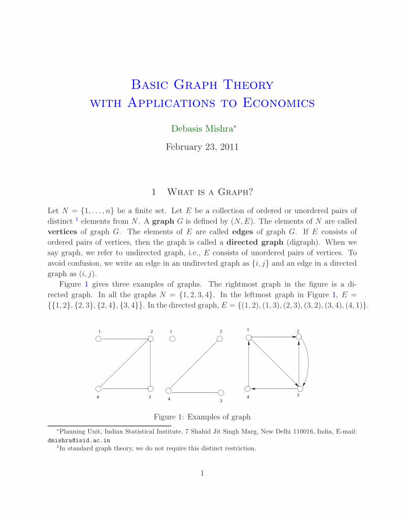

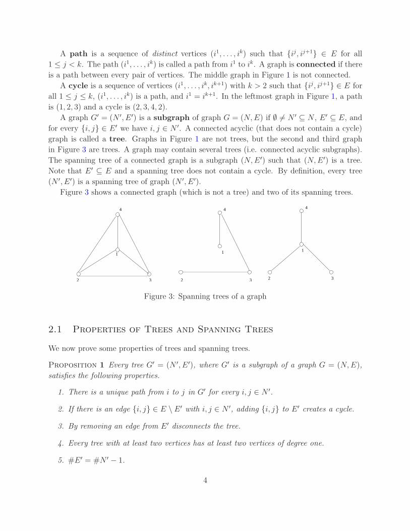
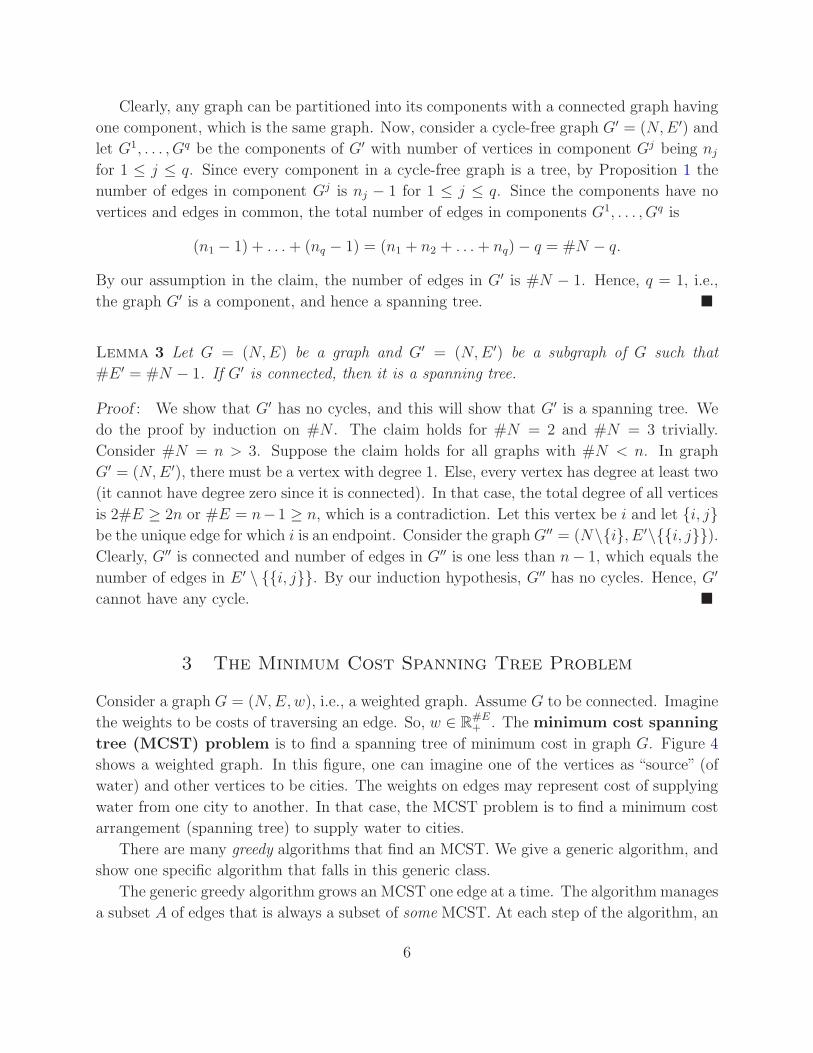
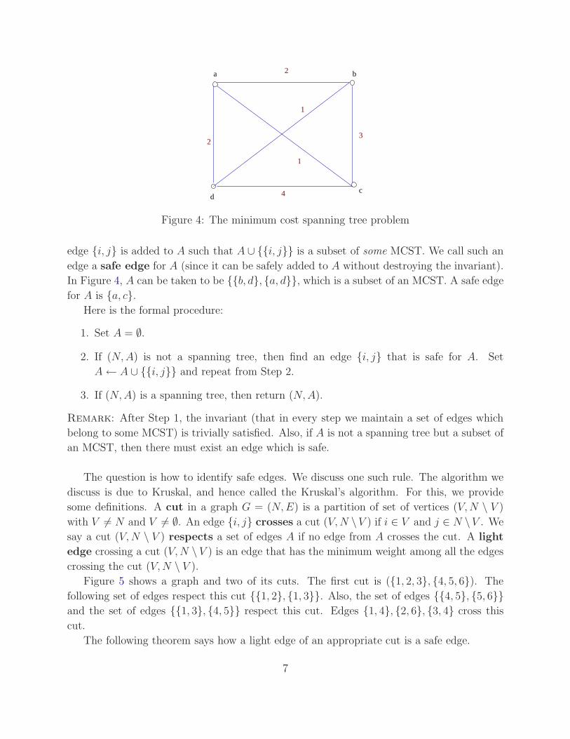


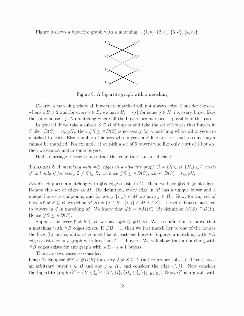
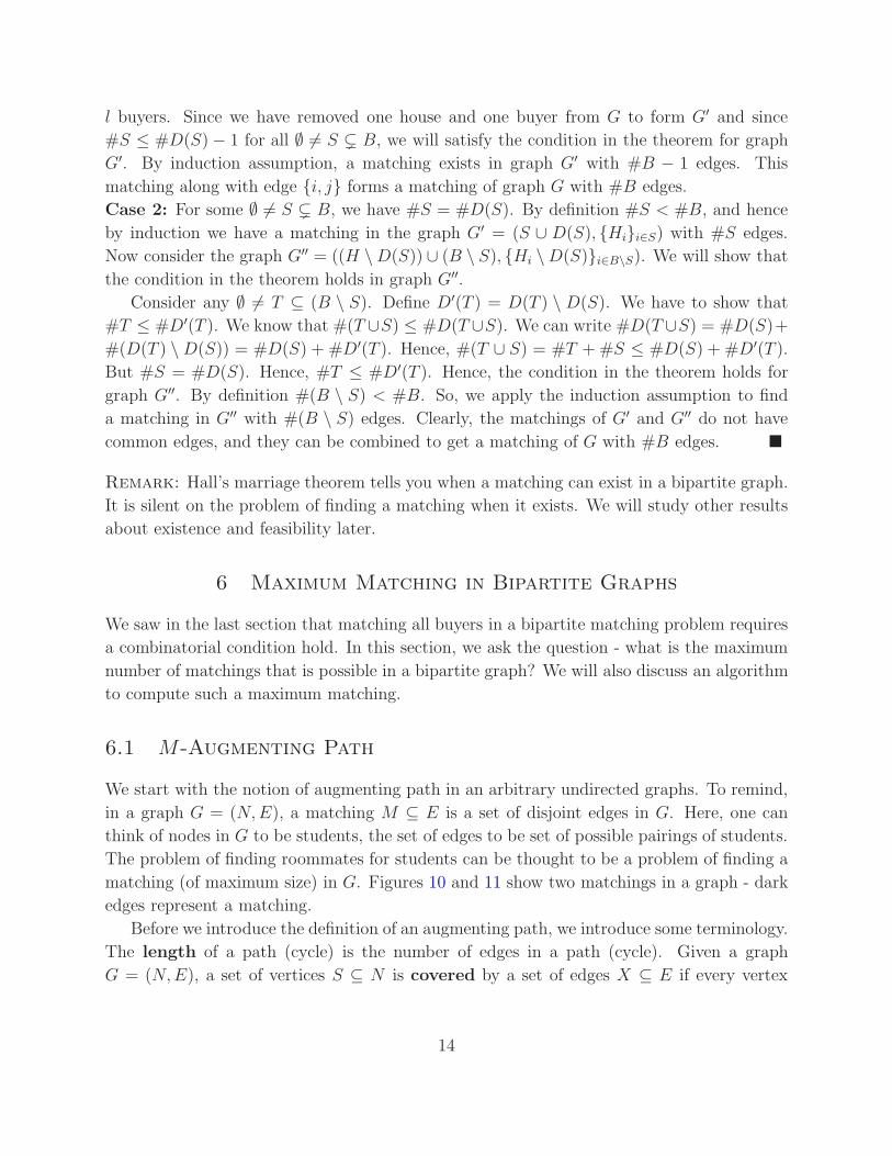
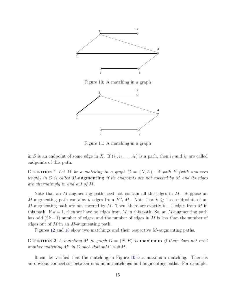


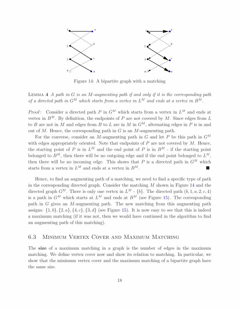


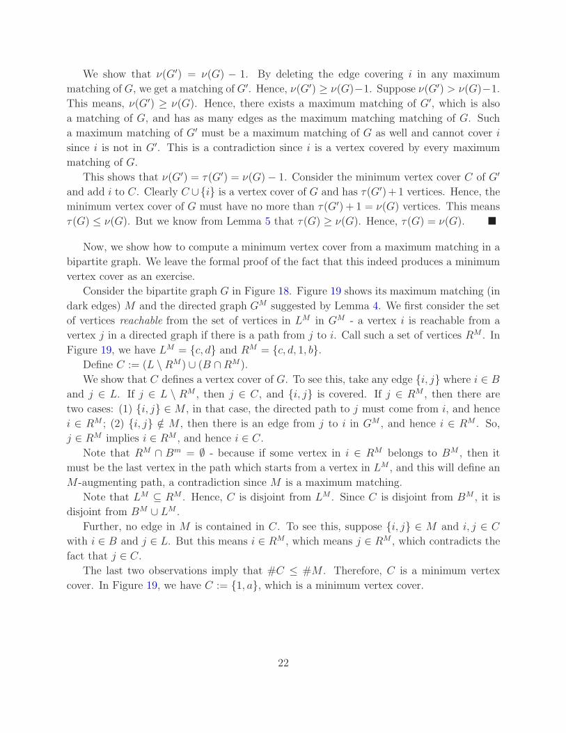

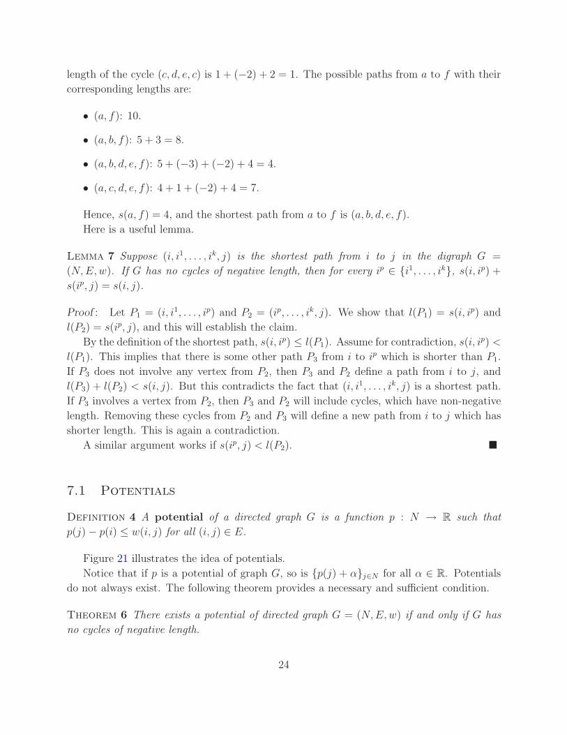

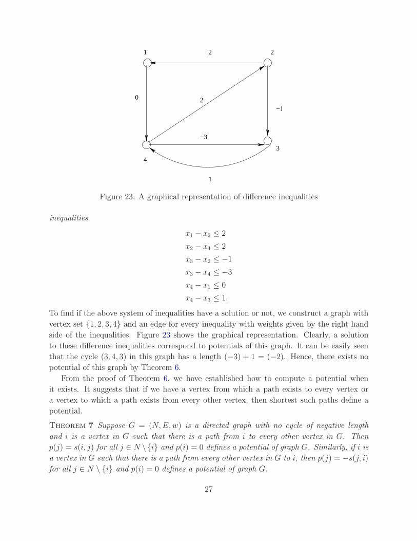


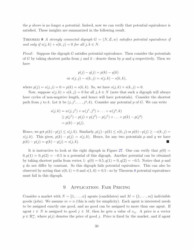

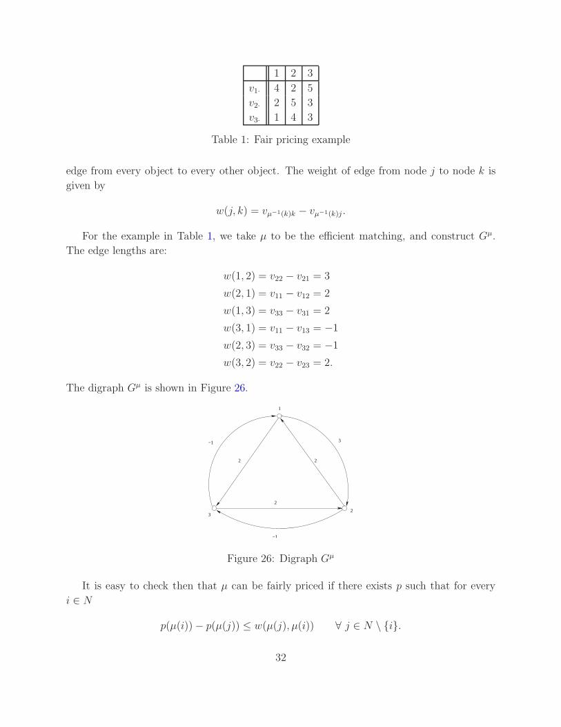
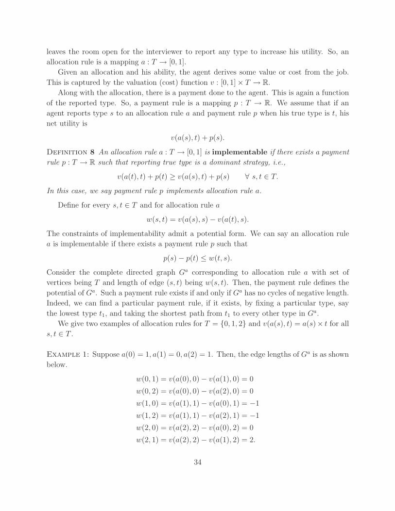

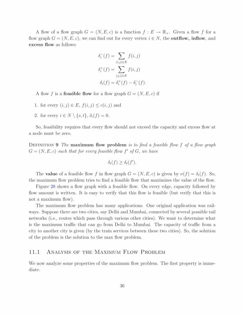
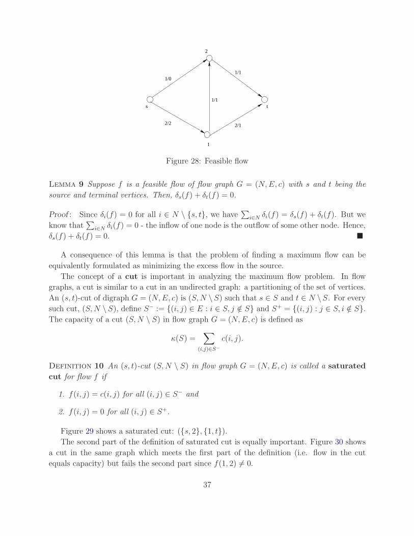

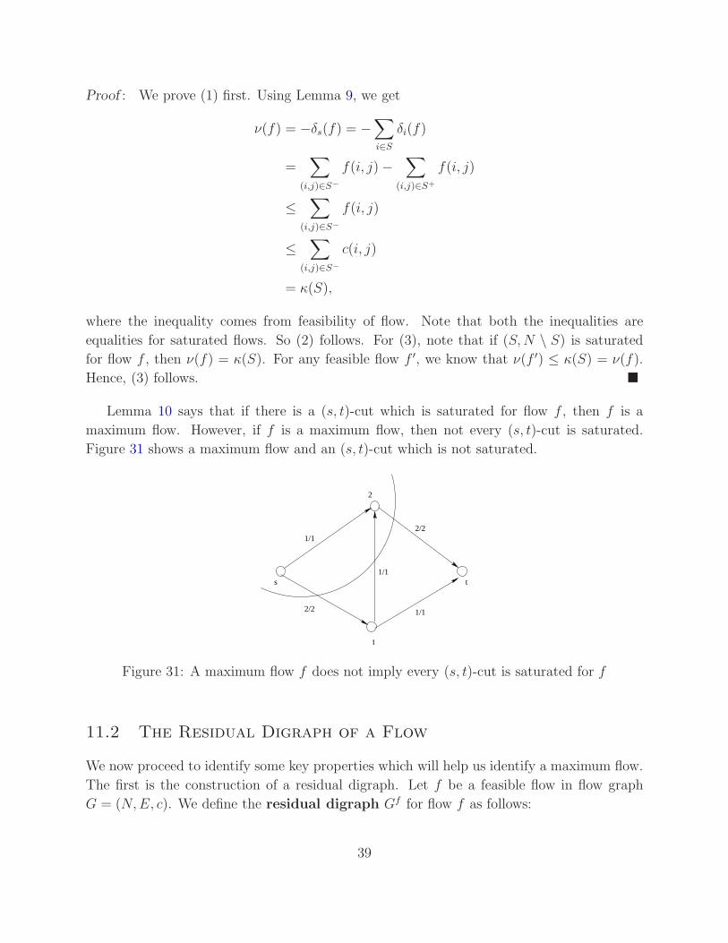


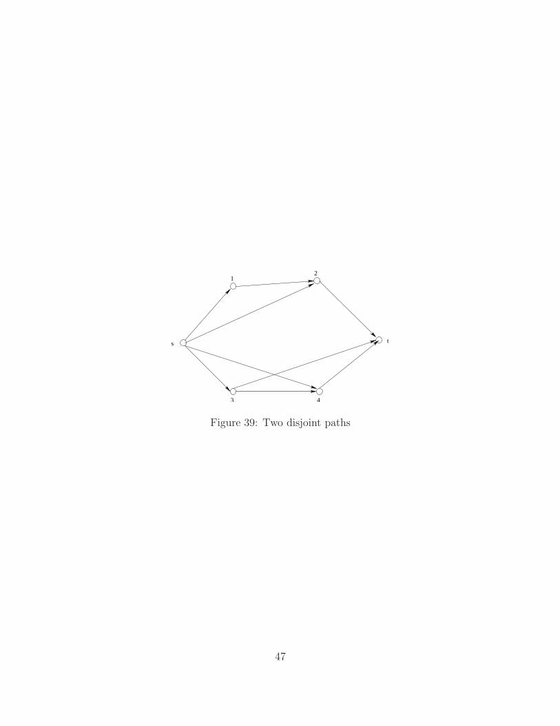


![Instruction Manual · Instruction Manual (App version 5.0+) 2019 Aug. 21 Bump Recorder Co., Ltd. 2 ... Advanced (front-side photography)”. Launch the app and open the [Graph] tab.](https://static.documents.pub/doc/80x56/60463a5aa4550a193c2a5f7c/instruction-manual-instruction-manual-app-version-50-2019-aug-21-bump-recorder.jpg)


