55
CASS-MT Task #7 - Georgia Tech GraphCT: A Graph Characterization Toolkit •David A. Bader, David Ediger, •Karl Jiang & Jason Riedy October 26, 2009
| Date post: | 24-Dec-2015 |
| Category: |
Documents |
| Upload: | juverianousheen |
| View: | 19 times |
| Download: | 0 times |

CASS-MT Task #7 - Georgia Tech
GraphCT:A Graph Characterization Toolkit
•David A. Bader, David Ediger,•Karl Jiang & Jason Riedy
October 26, 2009

Outline
Motivation
What is GraphCT?Package for Massive Social Network Analysis
Can handle graphs with billions of vertices & edges
Key FeaturesCommon data structure
A “buffet” of functions that can be combined
Using GraphCT
Future of GraphCT
Function Reference

Driving Forces in Social Network Analysis
An explosion of data!
300 million active Facebook users worldwide
in September 2009

Current Social Network Packages
UCINet, Pajek, SocNetV, tnetWritten in C, Java, Python, Ruby, RLimitations
Runs on workstation
Single-threaded
Several thousand to several million vertices
Low density graphs
We need a package that will easily accommodate graphs with several billion vertices on large, parallel machines

The Cray XMT
Tolerates latency by massive multithreadingHardware support for 128 threads on each processorGlobally hashed address spaceNo data cache Single cycle context switchMultiple outstanding memory requests
Support for fine-grained,
word-level synchronizationFull/empty bit associated with every
memory word
Flexibly supports dynamic load balancing
GraphCT currently tested on a 64 processor XMT: 8192 threads512 GB of globally shared memory
Image Source: cray.com

What is GraphCT?
Graph Characterization Toolkit
Efficiently summarizes and analyzes static graph data
Built for large multithreaded, shared memory machines like the Cray XMT
Increases productivity by decreasing programming complexity
Classic metrics & state-of-the-art kernels
Works on all types of graphsdirected or undirected
weighted or unweighted
Dynamic spatio-temporal graph

Key Features of GraphCT
Low-level primitives to high-level analytic kernelsCommon graph data structureDevelop custom reports by mixing and matching functionsCreate subgraphs for more in-depth analysisKernels are tuned to maximize scaling and performance (up to 64 processors) on the Cray XMT
Load the Graph Data Find Connected Components Run k-Betweenness Centralityon the largest component

Static graph data structure
typedef struct {int numEdges;int numVertices;int startVertex[NE]; /* start vertex of edge,
sorted, primary key */int endVertex[NE]; /* end vertex of edge,
sorted, secondary key */int intWeight[NE]; /* integer edge weight */
int edgeStart[NV]; /* per-vertex index into endVertex array */
int marks[NV]; /* common array for marking or coloring of vertices
*/} graph;

Using GraphCT

Usage options
Operations on input graphs can be specified in 3 ways:Via the command line
Perform a single graph operation
Read in graph, execute kernel, write back result
Via a script [in progress]
Batch multiple operations
Intermediate results need not be written to file (though they can be)
Via a developer’s API
Perform complex series of operations
Manipulate data structures
Implement custom functions

The command line interface
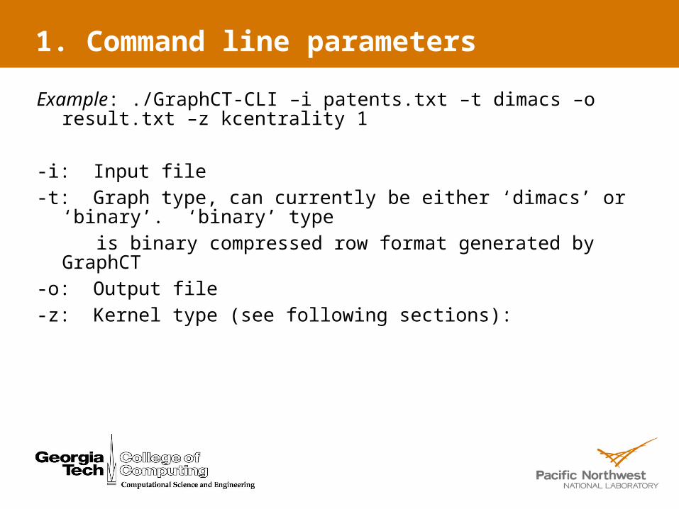
1. Command line parameters
Example: ./GraphCT-CLI –i patents.txt –t dimacs –o result.txt –z kcentrality 1
-i: Input file
-t: Graph type, can currently be either ‘dimacs’ or ‘binary’. ‘binary’ type
is binary compressed row format generated by GraphCT
-o: Output file
-z: Kernel type (see following sections):
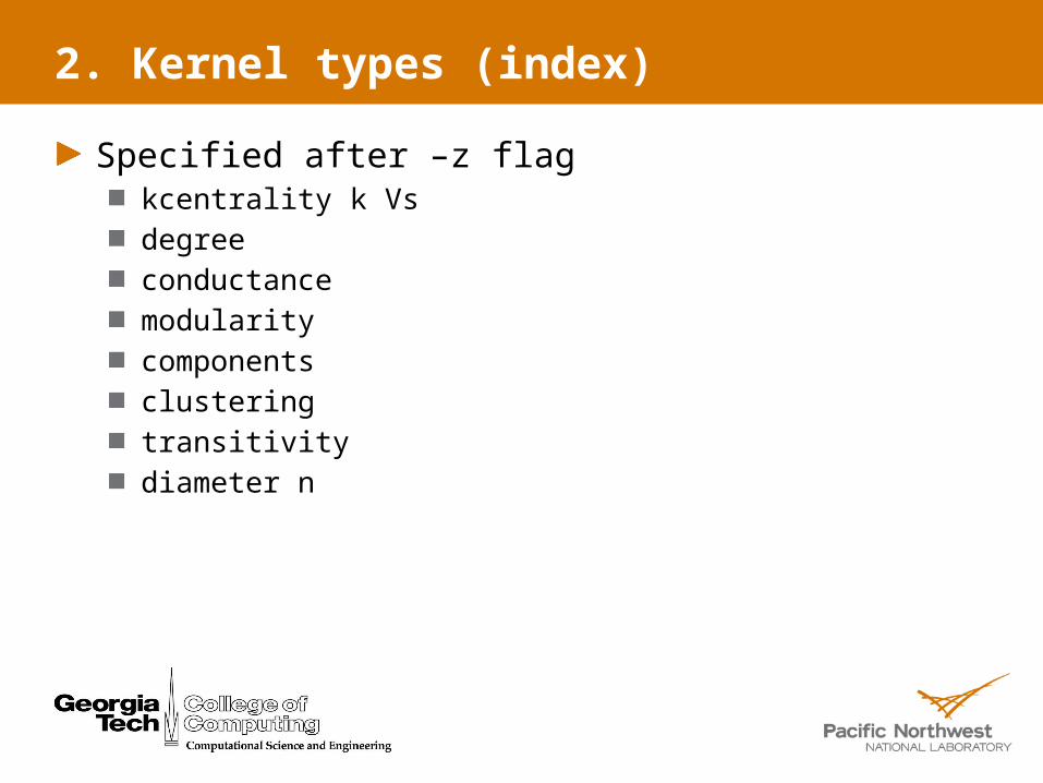
2. Kernel types (index)
Specified after –z flagkcentrality k Vs degreeconductancemodularitycomponentsclusteringtransitivitydiameter n

3. Degree distribution & graph diameter
Diameter can only be ascertained by repeatedly performing breadth first searches different vertices.
The more breadth first searches, the better approximation to the true diameter
-z diameter <P>Does breadth first searches from P percent of the vertices, where P is an integer
Degree distribution:-z degree: gives
Maximum out-degree
Average out-degree
Variance
Standard deviation

4. Conductance and modularity
-z conductance, -z modularity
Defined over colorings of input graphDescribe how tightly knit communities divided by a cut are
Not very meaningful in command line mode
In batch mode a coloring can be followed by conductance/modularity calculation
In batch mode:Finds connected components
Modularity uses component coloring as a partition
Conductance uses the largest component as the cut
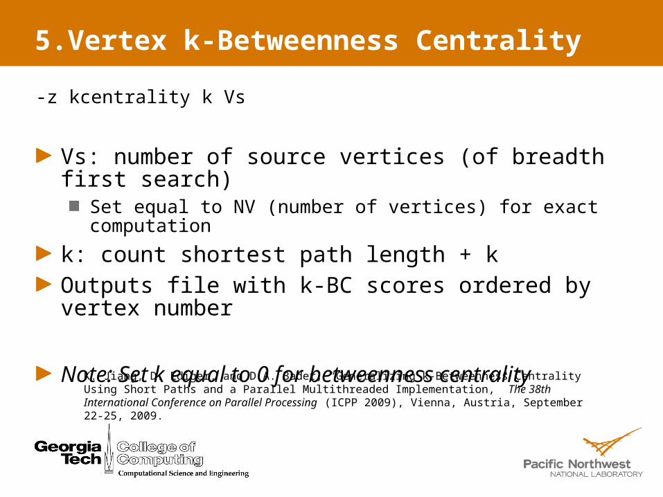
5.Vertex k-Betweenness Centrality
-z kcentrality k Vs
Vs: number of source vertices (of breadth first search)Set equal to NV (number of vertices) for exact computation
k: count shortest path length + kOutputs file with k-BC scores ordered by vertex number
Note: Set k equal to 0 for betweenness centrality
K. Jiang, D. Ediger, and D.A. Bader, “Generalizing k-Betweenness Centrality Using Short Paths and a Parallel Multithreaded Implementation,” The 38th International Conference on Parallel Processing (ICPP 2009), Vienna, Austria, September 22-25, 2009.

6. Transitivity/clustering coefficient
-z transitivity
Writes output file with local transitivity coefficient of each vertex
Measures number of transitive triads over total number of transitive triples
-z clustering
Writes output file with local clustering coefficient of each vertex
Number of triangles formed by neighbors over number of potential triangles
Gives sense of how close vertex is to belonging to a clique
Tore Opsahl and Pietro Panzarasa. “Clustering in weighted networks,” Social Networks, 31(2):155-163, May 2009.

7. Component statistics
-z components
Statistics about connected components in graphNumber of componentsLargest component sizeAverage component sizeVarianceStandard deviation
Writes output file with vertex to component mapping

Writing a script file [in progress]

1. Example script
read dimacs patents.txt => binary_pat.binprint diameter 10save graphextract component 1 => component1.binprint degreeskcentrality 1 256 => k1scores.txtkcentrality 2 256 => k2scores.txtrestore graphextract component 2print degrees

2. Script fundamentals
Work on single ‘active graph’Can save and restore graphs at any point, like memory feature on pocket calculatorOperations can:
Output data to the screen (e.g. degree information)
Output data to file (e.g. kcentrality data)
Modify the active graph (extract subgraph, component)

3. Example breakdown
read dimacs patents.txt => binary_pat.binTwo operations: reads in ‘patents.txt’ as a dimacs graph file, and writes the resulting graph back out as a binary file called ‘binary_pat.dat’
Binary graph is usually smaller and quicker to load
=> filename always takes the output of a particular command and writes it to the file ‘filename’
Current graph formats are ‘dimacs’ and ‘binary’
print diameter 10print command is used to print information to the screen
Shows the estimated diameter based on BFS runs from 10% of vertices

3. Example breakdown (cont.)
save graphRetain the current active graph for use later
extract component 1 => component1.binextract command is used to use a coloring to extract a subgraph from the active graph
component 1 colors the largest connected component
Writes resulting graph to a binary file
print degreesAny kernel from the previous section may be usedIf output is a graph or per-vertex data, it cannot be printed

3. Example breakdown (cont.)
kcentrality 1 256 => k1scores.txtCalculates k=1 betweenness centrality based on breadth first searches from 256 source vertices
Result stored in ‘k1scores.txt’, one line per vertex
kcentrality result cannot be printed to screen since it is per-vertex data
restore graphRestore active graph saved earlierCan restore same graph multiple times

3. Example breakdown (cont.)
extract component 2Extract the second largest component of the graph

Graph parsers
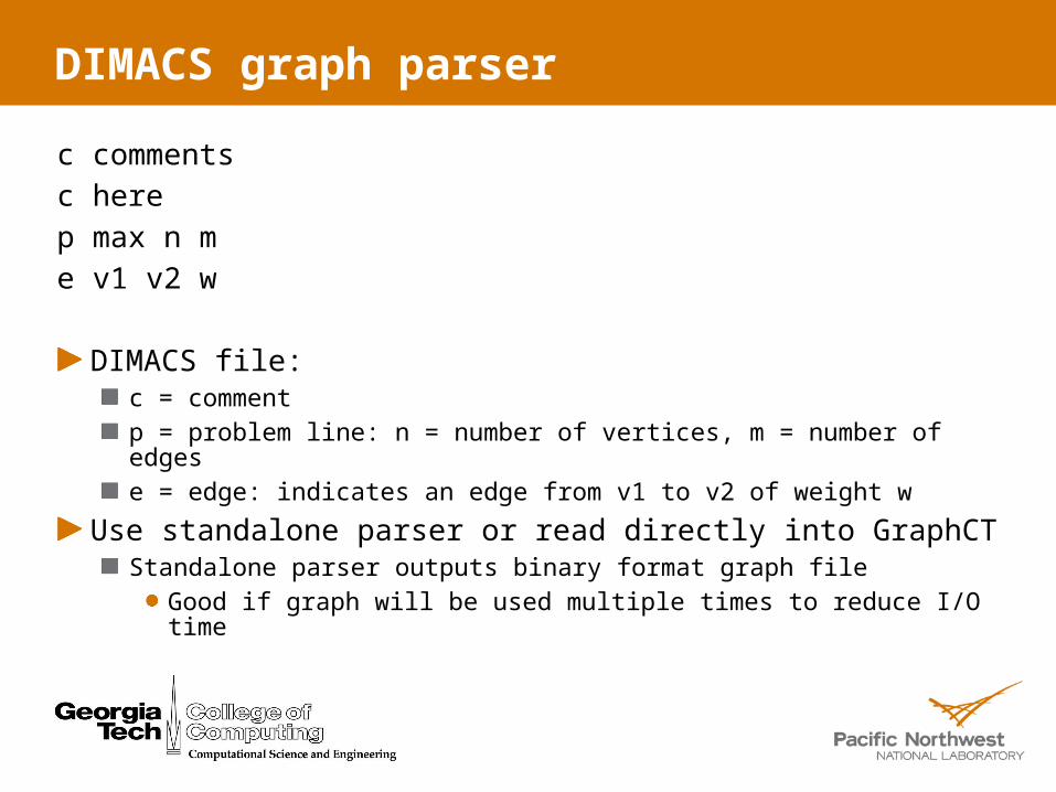
DIMACS graph parser
c commentsc herep max n me v1 v2 w
DIMACS file:c = comment
p = problem line: n = number of vertices, m = number of edges
e = edge: indicates an edge from v1 to v2 of weight w
Use standalone parser or read directly into GraphCTStandalone parser outputs binary format graph file
Good if graph will be used multiple times to reduce I/O time

From data to analysis
GraphCT produces a simple listing of the metrics most desired by the analyst
At a glance, the size, structure, and features of the graph can be described
Output can be custom tailored to show more or less data
Full results are written to files on disk for per-vertex kernels
k-Betweenness CentralityLocal clustering coefficientsBFS distance
Excellent for external plotting & visualization software

The Future of GraphCT
Additional high-level toolsDivisive betweenness-based community detection
Greedy agglomerative clustering (CNM)
Hybrid techniques
Additional subgraph generators
Helper functionsData pre-processing
Support for common graph formats
Extension to support dynamic graph dataSTINGER example

Experimental Kernels

Random walk subgraph extraction
Choose a number of random starting vertices nSG
Perform a BFS of length subGraphPathLength from each source vertex
Extract the subgraph:
void findSubGraphs(graph *G, int nSG, int subGraphPathLength)
subG = genSubGraph(G, NULL, 1);

Developer’s Notes:
A Programming Example

1. Initialization & graph generation
// I want a graph with ~270 million verticesgetUserParameters(28);
// Generate the graph tuples using RMATSDGdata = (graphSDG*) malloc(sizeof(graphSDG));genScalData(SDGdata, 0.57, 0.19, 0.19, 0.05);
// Build the graph data structureG = (graph *) malloc(sizeof(graph));computeGraph(G, SDGdata);

2. Degree distribution & graph diameter
// Display statistics on the vertex out-degreecalculateDegreeDistributions(G);
// Find the graph diameter exactlycalculateGraphDiameter(G, NV);// This will require 270M breadth first searches!
// Estimate the graph diametercalculateGraphDiameter(G, 1024);// This only does 1024 breadth first searches
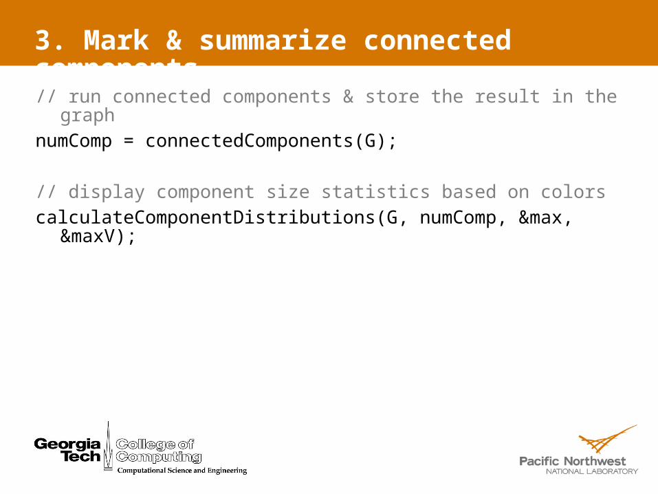
3. Mark & summarize connected components
// run connected components & store the result in the graph
numComp = connectedComponents(G);
// display component size statistics based on colorscalculateComponentDistributions(G, numComp, &max,
&maxV);

4. Find 10 highest 2-betweenness vertices
BC = (double *) malloc(NV * sizeof(double));
// k=2, 256 source verticeskcentrality(G, BC, 256, 2);
printf("Maximum BC Vertices\n");for (j = 0; j < 10; j++) { maxI = 0; maxBC = BC[0]; for (i = 1; i < NV; i++)
if (BC[i] > maxBC) {maxBC = BC[i]; maxI = i;} printf("#%2d: %8d - %9.6lf\n", j+1, maxI, maxBC); BC[maxI] = 0.0;}

Function Reference
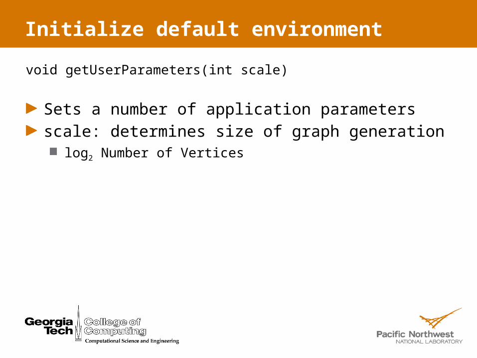
Initialize default environment
void getUserParameters(int scale)
Sets a number of application parametersscale: determines size of graph generation
log2 Number of Vertices

Load external graph data
int graphio_b(graph *G, char *filename)
Load from a binary data file containing compressed data structure using 4-byte integersFormat:
Number of Edges (4 bytes)Number of Vertices (4 bytes)Empty padding (4 bytes)edgeStart array (NV * 4 bytes)endVertex array (NE * 4 bytes)intWeight array (NE * 4 bytes)

Scalable data generator
void genScalData(graphSDG*, double a, double b, double c, double d)
Input:RMAT parameters A, B, C, & D
Must call getUserParameters( ) prior to calling this function
Output:graphSDG data structure (raw tuples)
Note: this function should precede a call to computeGraph() to transform tuples into a graph data structure
D. Chakrabarti, Y. Zhan, and C. Faloutsos. “R-MAT: A recursive model for graph mining”. In Proc. 4th SIAM Intl. Conf. on Data Mining (SDM), Orlando, FL, April 2004. SIAM.

Graph construction
void computeGraph(graph *G, graphSDG *SDGdata)
Input:graphSDG data structure
Output:graph data structure
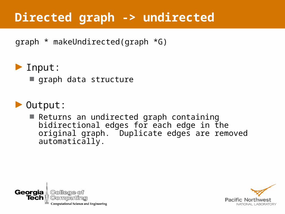
Directed graph -> undirected
graph * makeUndirected(graph *G)
Input:graph data structure
Output:Returns an undirected graph containing bidirectional edges for each edge in the original graph. Duplicate edges are removed automatically.

Generate a subgraph
graph * genSubGraph(graph *G, int NV, int color)
Input:graph data structure (marks[] must be set)
NV should always be set to NULL
color of vertices to extract
Output:Returns a graph containing only those vertices in the original graph marked with the specified color

K-core graph reduction
graph * kcore(graph *G, int K)
Input:graph data structure
minimum out-degree K
Output:Returns a graph containing only those vertices in the original graph with an out-degree of at least K

Vertex k-Betweenness Centrality
double kcentrality(graph *G, double BC[], int Vs,int K)
Vs: number of source verticesSet equal to G->NV for an exact computation
K: count shortest path length + KBC[ ]: stores per-vertex result of computation
Note: Set K equal to 0 for betweenness centrality
K. Jiang, D. Ediger, and D.A. Bader, “Generalizing k-Betweenness Centrality Using Short Paths and a Parallel Multithreaded Implementation,” The 38th International Conference on Parallel Processing (ICPP 2009), Vienna, Austria, September 22-25, 2009.

Degree distribution statistics
void calculateDegreeDistributions(graph*)
Input:graph data structure
Output:Maximum out-degreeAverage out-degreeVarianceStandard deviation

Component statistics
void calculateComponentDistributions (graph *G,int numColors, int *max, int *maxV)
Input:graph data structure
numColors: largest integer value of the coloring
Output:max: size of the largest component
maxV: an integer ID within the largest component

Modularity score
double computeModularityValue(graph *G,int membership[], int numColors)
Input:graph data structure
membership[]: the vertex coloring (partitioning)
numColors: the number of colors used above
Output:Modularity score is returned

Conductance score
double computeConductanceValue(graph *G,int membership[])
Input:graph data structure
membership[]: a binary partitioning
Output:Conductance score is returned

Connected components
int connectedComponents(graph *G)
Input:graph data structure
Output:G->marks[] : array containing each vertex’s coloring where each component has a unique color
Returns the number of connected components

Breadth first search
int * calculateBFS(graph *G, int startV, int mode)
Input:graph data structure
startV: vertex ID to start the search from
mode:
mode = 0: return an array of the further vertices where the first element is the number of vertices
mode = 1: return an array of the distances from each vertex to the source vertex
Output:Returns an array according to the mode described above
D.A. Bader and K. Madduri, “Designing Multithreaded Algorithms for Breadth-First Search and st-connectivity on the Cray MTA-2,” The 35th International Conference on Parallel Processing (ICPP 2006), Columbus, OH, August 14-18, 2006.

Graph diameter
int calculateGraphDiameter(graph *G, int Vs)
Input:graph data structure
Vs: number of breadth-first searches to run
Output:Returns the diameter (if Vs = NV) or the length of the longest path found
Note: this can be used to find the exact diameter or an approximation if only a subset of source vertices is used

Global transitivity coefficient
double calculateTransitivityGlobal(graph *G)
Input:graph data structure
Output:Returns the global transitivity coefficient (for both directed and undirected graphs)
Tore Opsahl and Pietro Panzarasa. “Clustering in weighted networks,” Social Networks, 31(2):155-163, May 2009.

Local transitivity coefficient
double * calculateTransitivityLocal(graph *G)
Input:graph data structure
Output:Returns the local transitivity coefficient for each vertex in an array
Tore Opsahl and Pietro Panzarasa. “Clustering in weighted networks,” Social Networks, 31(2):155-163, May 2009.

Local clustering coefficient
double * calculateClusteringLocal(graph *G)
Input:graph data structure
Output:Returns the local clustering coefficient for each vertex in an array
Tore Opsahl and Pietro Panzarasa. “Clustering in weighted networks,” Social Networks, 31(2):155-163, May 2009.


