James Madison UniversityJMU Scholarly Commons

Senior Honors Projects, 2010-current Honors College

Spring 2014

Graphical calculation of the fractal dimension forapplications in geographyLeeanne Nathalie JacksonJames Madison University

Follow this and additional works at: https://commons.lib.jmu.edu/honors201019

This Thesis is brought to you for free and open access by the Honors College at JMU Scholarly Commons. It has been accepted for inclusion in SeniorHonors Projects, 2010-current by an authorized administrator of JMU Scholarly Commons. For more information, please contactdc_admin@jmu.edu.

Recommended CitationJackson, Leeanne Nathalie, "Graphical calculation of the fractal dimension for applications in geography" (2014). Senior HonorsProjects, 2010-current. 431.https://commons.lib.jmu.edu/honors201019/431

Graphical Calculation of the Fractal Dimension

for Applications in Geography

_______________________

A Project Presented to

the Faculty of the Undergraduate

College of Integrated Science and Engineering

James Madison University

_______________________

in Partial Fulfillment of the Requirements

for the Degree of Bachelor of Science _______________________

by Leeanne Nathalie Jackson

May 2014

Accepted by the faculty of the Department of Integrated Science and Technology, James Madison University, in

partial fulfillment of the requirements for the Degree of Bachelor of Science.

FACULTY COMMITTEE:

Project Advisor: Dr. Helmut Kraenzle, Ph.D.,

Professor, Geographic Science

Reader: Dr. David Bernstein, Ph.D.,

Professor, Computer Science

Reader: Dr. Zachary Bortolot, Ph.D.,

Associate Professor, Geographic Science

HONORS PROGRAM APPROVAL:

Barry Falk, Ph.D.,

Director, Honors Program

2

Table of Contents

Acknowledgements 4

Abstract 5

Purpose and Objective 6

Literature Review 7

Methodology 11

Results 26

Discussion 30

Future Work 31

Appendix 32

Bibliography 50

3

List of Figures

1. Calculating the fractal dimension of an object with the box counting method. Image

from Kraenzle 1992 9

2. A UML Conceptual Class Diagram representing the overall

structure of the design 11

3. A UML Class Diagram specifying the attributes and functions

of the LineFeature class 13

4. A UML Class Diagram specifying the attributes and functions

of the Grid class 15

5. A UML Class Diagram specifying the attributes and functions

of the Cell class 17

6. A UML Class Diagram specifying the attributes and functions

of the LineSegment class 19

7. A UML Class Diagram specifying the attributes and functions

of the Point class 21

8. An image displaying 3 different levels of iteration of the Koch fractal. Obtained from

https://www2.southeastern.edu/Academics/Faculty/jbell/fractals.html 23

9. An image displaying several levels of iteration of the Sierpinski triangle. Obtained

from http://math.bu.edu/DYSYS/chaos-game/node2.html 24

10. U.S. zip code 22407, ESRI U.S. Zip Code Areas 24

11. Above: The original U.S. Zip Code 22407 and its vertices, as obtained from ESRI

Below: The simplified zip code region, with significantly fewer vertices 25

12. Program output and percent error for the Koch fractal 27

13. Program output and percent error for the Sierpinski fractal 28

14. Program output and percent error for U.S. Zip Code 22407 29

4

Acknowledgements

I would like to thank my advisor, Dr. Helmut Kraenzle, for his continued support and

guidance throughout the course of this project. I would also like to thank Dr. David Bernstein,

who has given me valuable technical support and project guidance.

5

Abstract

One metric that may be useful to geographers, especially in the study of natural features,

such as coastlines or animal habitats, is the fractal dimension. This statistic measures the

complexity of a feature, and can help researchers to predict patterns in data or to improve

existing datasets. The goal of this project was to create an application that graphically calculates

the fractal dimension of geographic features, and which may be added to the existing set of

technological tools used by geographers.

The method chosen for this algorithm to graphically calculate the fractal dimension was

to perform a functional box count. This involves overlaying a grid on the feature being examined

and counting the number of cells that intersect the shape. An object-oriented Python program

was designed and developed to represent geographic features in a vector format, and to

recursively calculate the fractal dimension. The design includes classes representing polygon and

linear curve features, as well as the points and line segments which make up these features.

The algorithm for calculating the fractal dimension has been tested for accuracy by

assessing its output using fractals with known and documented fractal dimensions. It has then

been applied to different geographic features to measure the dimension as an indicator of various

measures of interest to geographers.

6

Purpose and Objective

Geographic Information Systems (GIS) include tools for storing, displaying, and

analyzing geographic data, including graphical representations of both man-made and natural

features. A wide range of tools and software are available for geographers to use in their study

of these features, and as new technologies are developed, the capabilities of analysis using GIS

continue to expand.

The capabilities of GIS are wide-ranging, some involving geographic features, some

involving the features’ attributes, and others involving both. This project is concerned with

measures of the geographic features themselves, and draws upon coordinate-based calculations.

Broadly speaking, there are three types of geographic features: zero-dimensional features

(points), one-dimensional features (lines and curves), and two-dimensional features (polygons).

Not surprisingly, there are different measures of interest for each type of geographic features.

Examples include slope and angle for one-dimensional features and area and symmetry for two-

dimensional features.

This project is concerned with one particular measure of one-dimensional features: the

fractal dimension. This statistic measures a feature’s complexity, and can help researchers in the

field to predict patterns in data or to improve existing datasets. The goal of this project is to

create an application that will graphically calculate the fractal dimension of geographic features,

and which may be added to the existing set of technological tools used by geographers.

7

Literature Review

Natural geographic features have long been difficult to model and represent with

traditional Euclidean geometry, due to their complexity and scale-dependent characteristics

(Duckham & Worboys, 2004). For example, if one were to examine an image of a feature such

as a river or coastline, increasing levels of detail may be noted as the feature is viewed at

increasingly finer scales. In addition, the characteristics of a feature that may be examined at this

finer scale resemble those of a coarser, more zoomed-out view of the feature (Duckham &

Worboys, 2004). This characteristic of geographic features is called “self-similarity”, and is best

represented using fractal geometry (Duckham & Worboys, 2004). Fractals differ from traditional

Euclidean geometry in that they are defined recursively rather than by direct description of their

characteristics (Duckham & Worboys, 2004). They are perfectly and infinitely self-similar, and

have been successfully used to represent both natural and man-made features since Benoit

Mandelbrot first pioneered the development of techniques to analyze these complex forms in

1982 (Knight, n.d.).

One measure which may be calculated when using fractal geometry as a model for

geographic features is the fractal dimension, which describes the complexity of a feature (Knight,

n.d.). For geographic applications, it may also be described as a measure of the degree to which

detail is revealed at different scales (Duckham & Worboys, 2004). Dimensions of shapes and

objects are generally represented as integers, with the topological dimension of a point being

zero, that of a line or curve being one, a surface being two, and a solid object being three (Knight,

n.d.). The fractal dimension includes values that lie between these traditional integer descriptions,

to allow more nuanced interpretation of the complexity of an object (Knight, n.d.). For example,

a linear feature that is complex enough to fill a large area of space, thus appearing surface-like,

may have a fractal dimension that is nearer to two than one (Knight, n.d.). In geographic areas of

8

study, the fractal dimension is a useful descriptor of the shape of features, and has been used for

a variety of applications, especially in the study of geologic and biological features (Duckham &

Worboys, 2004). For example, Corbit and Garbary (1995) calculated the fractal dimension of the

forms of brown algae colonies to measure their levels of complexity, which allowed them to

predict their stages of development using raster images. In an interesting application to human-

made features, Knight (n.d.) proposed that the fractal dimension be used as a measure of

compactness and compared it to other traditional measures of this characteristic to examine

voting districts in the United States. The fractal dimension gives geographers and other scientists

a way to quantitatively describe features to uncover patterns which could not be observed using

traditional geometry.

One common method cited by researchers for graphically calculating the fractal

dimension is to perform a functional box count (Knight, n.d.). A grid is overlaid on the feature

being examined, and the number of cells that intersect the shape are counted. This is performed

using varying grid sizes, decreasing in size with each succession (Knight, n.d.). In this way, the

rapidity with which the length of the shape increases when examined at increasingly fine levels

of detail may be detected (Knight, n.d.). Data including the box count and the size of the boxes,

when logged and plotted on a graph, should form a log-linear pattern with the following

relationship:

( ) ( )

where C denotes the box count and S denotes the box size. Using this formula, the fractal

dimension is represented by the absolute value of b, or the slope of the line (Knight, n.d.).

Kraenzle used fractal models to generate coastlines and applied the box counting method to

calculate the fractal dimension of various coastlines (Fig. 1, Kraenzle, 1992).

9

Figure 1. Calculating the fractal dimension of an object with the box counting method. Image

from Kraenzle 1992

As the box-counting method for calculating the fractal dimension is inherently graphical,

development of an algorithm for this purpose requires a choice of how to represent the features.

Computer graphics may be stored in both vector formats, which store information about the

shapes of features in the form of coordinates making up lines or polygons, and raster formats,

which store an array of pixels to represent an image. Vector formats are used most often to

10

represent geographic features, while raster formats are often associated with data values

corresponding to a grid of coordinates on the ground. Raster formats are often used when data

comes from a source such as satellite or aerial photography. The box-count method of

calculating the fractal dimension has been used by geographers to analyze features stored with

both of these data types (Ran, 2008). For the algorithm described below, a vector data format

was chosen to represent the fractal and geographic features due to the speed and ease of

performing spatial operations and the linear format of the features of interest.

11

Methodology

A program was developed in Python using the Eclipse PyDev environment to represent

vector objects necessary for calculating the fractal dimension of a shape.

High-Level Algorithm Design

Figure 2. A UML Conceptual Class Diagram representing the overall structure of the design.

An object-oriented design was developed to represent vector objects necessary for

calculating the fractal dimension of a fractal or geographic feature, incorporating the following

classes:

LineFeature

This class represents a vector feature which is made up of LineSegment objects.

Objects of this class represent the feature for which the fractal dimension is of interest. These

features may be imported from an ArcGIS feature class, or represents another type of shape, such

as a fractal. Though the first and last Point of a LineFeature object can refer to the same location,

all LineFeature objects are one-dimensional. A LineFeature has a length, but not an area. Though

a LineFeature object, when rendered, might appear to be the border of a polygon, it is not a

polygon.

12

Grid

The Grid class represents a set of grid cells (Cell objects) which are contained within

the bounding box of a given shape. This class depends on a LineFeature object to supply it

with a bounding box upon which it is constructed. The grid is necessary for the box-counting

algorithm used to calculate the fractal dimension. A Grid object is always square and its

boundary length is equal to the length of the longest side of the associated LineFeature’s

bounding box.

Cell

A Cell object represents one cell which is part of a Grid object. A Cell is composed

of four line segments representing its square boundary, and is used in the box-counting algorithm

to determine whether a given line segment intersects, or is contained within, its boundaries.

LineSegment – A LineSegment object contains two Point objects representing a starting

point and an endpoint. LineSegments are components of LineFeature and Cell objects.

The key behavior of a LineSegment is the ability to determine whether it intersects with

another LineSegment. This is the foundation for the line-cell intersection logic used in the box-

counting algorithm.

Point – Point objects represent vectors which contain an x-coordinate and a y-coordinate, and

they make up the endpoints of LineSegment objects. Point objects are also used to represent

the coordinates of a LineFeature or Grid’s bounding box.

13

Individual Class Documentation

Figure 3. A UML Class Diagram specifying the attributes and functions of the LineFeature class.

The LineFeature class represents a piecewise linear curve. It is composed of a series of

connected LineSegment objects, and its main purpose is to calculate the fractal dimension of

the linear feature.

Attributes:

_lines – Contains a list of LineSegment objects which make up the LineFeature.

_boundingBox – Contains the bounding coordinates of the LineFeature, stored as a list of

two Point objects in the following format: [MinPoint, MaxPoint]

_grid – Contains the Grid object associated with this feature, which is created upon

instantiation of a LineFeature object. The boundaries of the Grid coincide with the bounding

box, originating from the box’s bottom-left point.

Methods:

__init__(lineSegments, fileName) – The constructor, which initializes all attributes.

The LineSegments which make up the curve can be provided either in the form of a list of

LineSegment objects, or in a comma-delimited text file containing coordinate values.

14

calcFractalDimension(iterations) – This method calculates the fractal dimension of

the LineFeature object. It uses the grid attribute to recursively perform a box count with a

user-specified number of iterations.

_boxCount(grid) –This helper method for calcFractalDimension performs a box count

on the LineFeature object using the Grid provided as an argument. It is called upon in each

iteration of the calcFractalDimension method to perform the count.

_calculateBox() – This method is called by the constructor to calculate the bounding box of

the LineFeature by calculating its minimum and maximum coordinates.

getLines() – This is an accessor method to retrieve the LineSegments which make up this

LineFeature.

15

Figure 4. A UML Class Diagram specifying the attributes and functions of the Grid class.

The Grid class represents a grid which overlays a LineFeature object – the bounding

box of the object is used to determine the Grid’s size. The Grid represents the grid of boxes

used in the box-counting algorithm, and includes attributes to keep track of the bounding box,

the cells which make up the grid, and the grid cell sizes in proportion to the overall grid height

and width. The Grid is stored as an attribute of a LineFeature object.

Attributes:

_cells – This is a list containing all the Cell objects which represent the cells of the grid.

_bound – This list contains two Point objects representing the bounding box of the grid. It is

in the format [minPoint, maxPoint].

_proportion – This integer represents the denominator of the fraction

, representing the

proportion of the width or height (whichever is larger) of the grid which is occupied by a single

cell. For example, if the grid is only one large cell (the bounding box), the proportion is 1. If the

grid was divided into 3 cells by 3 cells (9 total), and each cell’s dimensions are

of that of the

grid, the proportion is 3.

16

_distance – This is a floating point value representing the length of one side of the square

grid.

_cellSize – This contains a floating point value representing the length of one side of any cell

in the grid.

Methods:

__init__(boundBox, proportion) – The constructor, which takes the coordinates of the

bounding box (a list of two Point objects) and an integer proportion value as arguments. The

proportion parameter determines how many cells will initially make up the grid. The constructor

sets the initial values for all attributes, creating the initial set of cells using the createCells()

method.

createCells(lowerLeft, distance, iterations, lowRight, upLeft,

upRight) – This method takes a Point object (lowerLeft) and creates a Cell object using

the distance parameter to calculate the location of the remaining three coordinates which make

up the Cell’s LineSegments. It then recursively calculates cells for the rest of the grid. The

parameter “iterations” is used to keep track of the number of cells which need to be created.

The remaining parameters are Boolean values which specify whether a new cell will need to be

created using one of the other points of this cell as its starting point.

refineGrid() – This method creates and returns a new Grid object with the same bounding

box, but with grid cells of half the width of the current Grid’s cells.

getDistance() – This is an accessor method for the length of one side of the Grid.

toString() – A method used to print the contents of a Grid object (describing all of the cells

which have been created). The primary purpose of this method is for debugging.

getCellSize() – This is an accessor method for the cell size of the Grid.

17

Figure 5. A UML Class Diagram specifying the attributes and functions of the Cell class.

The Cell class represents one cell in a Grid object. The cell is square in shape, and is

made up of four LineSegments, representing the top, bottom, left, and right boundaries of the

square. A Cell is constructed from four line segments, and contains a function determining

whether another LineSegment is intersecting the area which the Cell occupies.

Attributes:

_top – The LineSegment which represents the top boundary of this Cell.

_bottom – The LineSegment which represents the bottom boundary of this Cell.

_left – The LineSegment which represents the left boundary of this Cell.

_right – The LineSegment which represents the right boundary of this Cell.

Methods:

__init__(top, bottom, left, right) – This method is the constructor, which takes in

the four line segments which make up this Cell as parameters. The LineSegment attributes

are initialized using these values.

18

intersects(line) – This method takes a single LineSegment as a parameter. It returns

true if the given LineSegment intersects the Cell, otherwise it returns false. Intersection is

defined as follows:

1. The LineSegment intersects any boundary line of the Cell, or

2. The LineSegment is completely contained within the Cell.

toString() – Prints the contents of the cell – the four LineSegments which make it up.

Primarily used for debugging.

19

Figure 6. A UML Class Diagram specifying the attributes and functions of the LineSegment

class.

A LineSegment represents one line segment which is a part of a LineFeature or

Cell. A LineSegment has a start Point and an end Point. It contains functions for accessing

these points, and determining whether the LineSegment intersects another LineSegment,

which is the basis for determining whether a LineSegment intersects a Cell.

Attributes:

_start – A Point object which represents the starting point of the LineSegment.

_end – A Point object which represents the end point of the LineSegment.

_slopeIsDefined – A Boolean value which is true if the slope has a defined value. In the

case where the x values of the start and end points of the line are equal, the slope is undefined

and cannot be used in calculations.

_slope – Contains the slope of the line, represented as a floating point value.

Methods:

__init__(start, end) – The constructor, which takes two Point objects as parameters:

the start and end points of the LineSegment. All attributes are initialized.

20

getStart() – Returns the start point of the LineSegment.

getEnd() – Returns the end point of the LineSegment.

intersects(other) – Takes a LineSegment as a parameter. Returns true if the

LineSegment which calls the method and the LineSegment which is the parameter intersect

one another, otherwise returns false.

toString() – Returns a string representation of this LineSegment, describing its start and

end points. Primarily used for debugging.

_findSlope() – This method is used by the constructor to determine if the slope is defined,

and to calculate the slope. It returns a floating point value representing the slope.

21

Figure 7. A UML Class Diagram specifying the attributes and functions of the Point class.

A Point represents one (x, y) coordinate pair, which is the start or end point of a

LineSegment object. The Point class contains attributes containing the x and y values. It also

contains functions for determining if the Point is greater than or less than another point in both

the x and y directions.

Attributes:

_xCoord – The x-coordinate of the Point.

_yCoord – The y-coordinate of the Point.

Methods:

__init__(xValue, yValue) – The constructor, initializes the coordinates of the point based

on the parameters xValue and yValue, which must be float values.

getX() – Returns the x-coordinate of the Point.

getY() – Returns the y-coordinate of the Point.

toString() – Returns a string representation of the Point, describing its coordinates.

Primarily used for debugging.

22

isGreater(other) – Compares the Point calling the method to another point, given as a

parameter, returning true if the x and y values of the first point are both greater than those values

of the second point. Primarily used to determine whether a LineSegment is contained within a

Cell.

isLess(other) – Compares the Point calling the method to another point, given as a

parameter, returning true if the x and y values of the first point are both less than those values of

the second point. This function is primarily used to determine whether a LineSegment is

contained within a Cell.

23

Study Design

The output of the program was tested using two fractals with known dimensions: the

Koch Snowflake Fractal (Fig. 8), with a dimension of 1.2618, and the Sierpinski Triangle (Fig.

9), with a dimension of 1.5849 (Mandelbrot, 1982). An algorithm to produce a text file

containing coordinates for the Koch fractal was provided by JMU undergraduate student Colin

Spohn, and the algorithm was run with four, five, and six iterations to generate fractals of

varying complexity to be used as input. The Sierpinski fractal was generated using an algorithm

which directly created a list of LineSegments to initialize a LineFeature object. The Sierpinski

fractal was also generated with four, five, and six iterations.

Figure 8. An image displaying 3 different levels of iteration of the Koch fractal. Obtained from

https://www2.southeastern.edu/Academics/Faculty/jbell/fractals.html

24

Figure 9. An image displaying several levels of iteration of the Sierpinski triangle. Obtained

from http://math.bu.edu/DYSYS/chaos-game/node2.html

The program’s output was also tested using one geographic feature, the boundary of U.S.

zip code 22407, isolated from ESRI’s U.S. Zip Code Areas (Five-Digit) dataset (Fig.10). The

vertices of this feature were exported from ArcGIS as a text file. A copy of this feature was made

and re-digitized with a smaller number of vertices to be used as a preliminary examination of the

difference in the fractal dimension based on the accuracy of digitization and complexity of a

feature.

Figure 10. U.S. zip code 22407, ESRI U.S. Zip Code Areas

25

The results of the algorithm using three different numbers of grid refinements (four, five,

and six iterations) were recorded for each vector object used. These numbers were chosen due to

the fact that the algorithm was limited to seven or fewer iterations, because eight or more

produced a stack overflow error due to the recursive nature of the function, which limits the

depth of calculations. The percent error of the output was then calculated to assess accuracy

using the following formula:

( )

Figure 11. Left: The original U.S. Zip Code 22407 and its vertices, as obtained from ESRI

Right: The simplified zip code region, with significantly fewer vertices.

26

Expected Results

Because the box-counting algorithm is designed so that more iterations of grid refinement

will produce an approximation which approaches the true fractal dimension, it is expected that

higher numbers of grid refinement iterations will produce output values which are closer to the

actual value. It should also occur that higher numbers of iterations when generating each fractal

will produce results closer to the actual fractal dimension, because a higher number of fractal

iterations more closely approximates the ideal infinite fractal.

With regard to the U.S. zip code feature, it is expected that the original and more

complex version of the feature, before vertices were simplified, would have a higher fractal

dimension value because the fractal dimension is a measure of complexity.

27

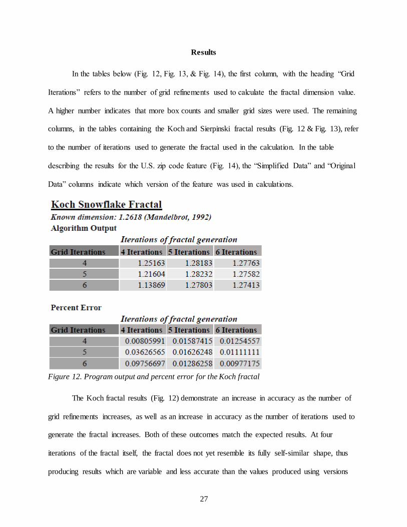
Results

In the tables below (Fig. 12, Fig. 13, & Fig. 14), the first column, with the heading “Grid

Iterations” refers to the number of grid refinements used to calculate the fractal dimension value.

A higher number indicates that more box counts and smaller grid sizes were used. The remaining

columns, in the tables containing the Koch and Sierpinski fractal results (Fig. 12 & Fig. 13), refer

to the number of iterations used to generate the fractal used in the calculation. In the table

describing the results for the U.S. zip code feature (Fig. 14), the “Simplified Data” and “Original

Data” columns indicate which version of the feature was used in calculations.

Figure 12. Program output and percent error for the Koch fractal

The Koch fractal results (Fig. 12) demonstrate an increase in accuracy as the number of

grid refinements increases, as well as an increase in accuracy as the number of iterations used to

generate the fractal increases. Both of these outcomes match the expected results. At four

iterations of the fractal itself, the fractal does not yet resemble its fully self-similar shape, thus

producing results which are variable and less accurate than the values produced using versions

28

with higher numbers of iterations. Higher numbers of fractal iterations produced less variable

results, when different numbers of grid refinements were used, than lower numbers of fractal

iterations.

Figure 13. Program output and percent error for the Sierpinski fractal

The Sierpinski fractal output (Fig. 13) is in agreement with the results of the Koch fractal

calculations in that higher numbers of iterations when generating the fractals produced generally

more accurate results, and that the output values varied less among the fractals which were

generated with a higher number of iterations than those generated with a lower number of

iterations. However, calculations using the Sierpinski fractal demonstrated that as the number of

grid refinements increased, the fractal dimension value decreased and moved further from the

correct value. This result is contrary to expectations.

29

Figure 14. Program output and percent error for U.S. Zip Code 22407

The original zip code data (Fig. 14), before being re-digitized and simplified, was shown

to have a higher fractal dimension than that of the simplified data at each level of grid iteration.

This result matches the expected outcome. An additional observation which can be drawn from

these data is that a higher number of grid iterations produced a smaller fractal dimension, when

each dataset is examined independently.

30

Discussion

The results of the Koch and Sierpinski fractal calculations demonstrate that running the

algorithm using fractals generated with higher numbers of iterations produce results which are

closer to the actual fractal dimension values. The results using the Koch fractal also support the

notion that running a higher number of grid refinements will produce a result that is increasingly

closer to the actual value. The results using the Sierpinski fractal contradicted this notion, as the

values decreased and moved away from the correct result as the number of grid refinements was

increased. However, this can be explained by the fact that the Sierpinski fractal represents a

polygonal shape, and the algorithm used only examines the linear boundary of the feature. As a

result, when the grid size becomes increasingly fine (as is the case with a higher number of

refinements), a smaller proportion of the grid’s boxes intersect the feature, because there are

large open spaces representing the triangles which would be counted if the polygon area was

taken into consideration. As a result, the Sierpinski fractal is best suited to area-based

calculations, and the values produced by the algorithm tested have limited accuracy.

Other observations to be made from the fractal results include the fact that there was less

variation in the output values when the fractals used were generated with a higher number of

iterations, and that the fractals generated with only four iterations were not yet close enough to

their mature shape to produce accurate results.

As was expected, the results of the zip code feature output suggest that there is positive

association between the complexity of the geographic data and the fractal dimension. At every

level of grid refinement, the more complex original dataset had a higher fractal dimension than

its simplified counterpart.

31

Future Work

Several additions could be made to the program developed in this project. The algorithm

currently only handles piecewise linear curve objects, and could be expanded to work with

polygon data, taking into account the area which is contained by the shape when performing the

box count. The program’s efficiency could also be studied, and its speed of execution could

likely be improved by changing the implementation of the recursive functions to use a loop.

Doing so would also remove the limitation on the number of iterations created by the recursion.

If this software was found to be accurate and useful as a GIS tool, a GUI could be developed and

the software could be distributed. It could also be extended to support GIS data formats such as

those used by ESRI.

One implication of the zip code data results is that the fractal dimension could be used as

a measure of data and digitization accuracy – a set of data which has been collected accurately

should be similar in complexity to a known accurate set of data, and further work on this subject

could bring to light a useful application of the fractal dimension to this area.

32

Appendix: Python Code

i. LineFeature Class (LineFeature.py)

'''

LineFeature.py

This class represents a line feature object, which is composed

of LineSegment objects.

Includes a method to calculate the fractal dimension.

Created by Leeanne Jackson, James Madison University

Last edited: March 28, 2014

'''

from LineSegment import LineSegment

from Point import Point

from Grid import Grid

import math

class LineFeature(object):

#Constructor - initialize variables

def __init__(self, lineSegments = None, fileName = None):

if lineSegments == None:

if fileName == None:

print "Please supply either a file name or a list of segments."

else:

coordFile = open(fileName, 'r')

self._lines = []

segment = []

line = coordFile.readline()

while line:

i = 0

n = len(line)

value = ""

pair = []

33

while i < n:

if line[i] != ",":

value = value + line[i]

else:

i = i + 1

break

i = i + 1

pair.append(float(value))

value = ""

while i < n:

if line[i] != "\n":

value = value + line[i]

i = i + 1

pair.append(float(value))

value = ""

segment.append(pair)

pair = []

line = coordFile.readline()

if len(segment) == 2:

self._lines.append(LineSegment(Point(segment[0][0], segment[0][1]),

Point(segment[1][0], segment[1][1])))

segment = []

self._boundingBox = self._calculateBox()

self._grid = Grid(self._boundingBox, 5)

else:

self._lines = lineSegments

self._boundingBox = self._calculateBox()

self._grid = Grid(self._boundingBox, 5)

#Returns fractal dimension value

#Parameter iterations: The number of iterations to refine

#the grid

def calcFractalDimension(self, iterations):

grid = self._grid

lines = []

points = []

34

proportion = 1

while iterations > 0:

print "Iterations remaining: ", iterations

count = self._boxCount(grid)

points.append(Point(math.log(1.0/grid.getCellSize()), math.log(count)))

grid = grid.refineGrid()

proportion = proportion * 2

iterations -= 1

x = 0

n = len(points)

while x < n:

if x < n - 1:

lines.append(LineSegment(points[x], points[x+1]))

else:

lines.append(LineSegment(points[x], points[0]))

x += 1

sum = 0.0

for z in lines:

if z._slopeIsDefined:

sum += z.getSlope()

return sum / len(lines)

#Helper method for calcFractalDimension - counts the cells

#in the given grid which intersect with this line feature object

def _boxCount(self, grid):

boxCount = 0

flag = False

for x in grid._cells:

flag = False

for y in self._lines:

if x.intersects(y):

boxCount += 1

flag = True

if flag:

35

break

return boxCount

#Helper method:

#Returns bounding box of the shape in the following format:

# [MinPoint, MaxPoint]

def _calculateBox(self):

minX = self._lines[0].getEnd().getX()

minY = self._lines[0].getStart().getY()

maxX = self._lines[0].getStart().getX()

maxY = self._lines[0].getStart().getY()

i = 0

n = len(self._lines)

while i < n:

start = self._lines[i].getStart()

end = self._lines[i].getEnd()

if start.getX() < minX:

minX = start.getX()

if start.getX() > maxX:

maxX = start.getX()

if end.getX() < minX:

minX = end.getX()

if end.getX() > maxX:

maxX = end.getX()

if start.getY() < minY:

minY = start.getY()

if start.getY() > maxY:

maxY = start.getY()

if end.getY() < minY:

minY = end.getY()

if end.getY() > maxY:

maxY = end.getY()

i += 1

36

box = [Point(minX, minY), Point(maxX, maxY)]

return box

#Accessor method for the LineSegment objects which make up

#this feature.

def getLines(self):

return self._lines

37

ii. Grid Class (Grid.py)

'''

Grid.py

This class represents a grid used in a box count to calculate the

fractal dimension of a feature. It is composed of Cell objects.

Includes methods for refining the grid cells.

Created by Leeanne Jackson, James Madison University

Last Edited: March 30, 2014

'''

from Cell import Cell

from Point import Point

from LineSegment import LineSegment

class Grid(object):

###

# Constructor

#

# boundBox

# The bounding box of the fractal to be contained

# by this grid. format [minPoint, maxPoint]

# proportion

# An int (x) representing the size of the cells in relation to the grid.

# cell = 1/x * (grid size)

###

def __init__(self, boundBox, proportion):

height = abs(boundBox[1].getY() - boundBox[0].getY())

width = abs(boundBox[1].getX() - boundBox[0].getX())

self._cells = []

self._bound = boundBox

38

if height > width:

self._distance = height

else:

self._distance = width

self._proportion = proportion

self._cellSize = self._distance / float(self._proportion)

self._createCells(boundBox[0], self._distance / float(proportion),

proportion - 1, True, True, True)

###

# Create a cell using its bottom-left point - a Point object

# Distance parameter is the length of one side of the cell

#

# Appends the new cell to the _cells attribute

#

# Parameters lowRight, upLeft, upRight are boolean values indicating which points in relation

# to this point should be calculated. For example, if the Cell is the upper-rightmost Cell in

# the Grid, no other cells will be calculated using its points

#

###

def _createCells(self, lowerLeft, distance, iterations, lowRight, upLeft, upRight):

lowerRight = []

upperLeft = []

upperRight = []

lowerRight = Point(lowerLeft.getX() + distance, lowerLeft.getY())

upperLeft = Point(lowerLeft.getX(), lowerLeft.getY() + distance)

upperRight = Point(lowerLeft.getX() + distance, lowerLeft.getY() + distance)

top = LineSegment(upperLeft, upperRight)

bottom = LineSegment(lowerRight, lowerLeft)

left = LineSegment(lowerLeft, upperLeft)

right = LineSegment(upperRight, lowerRight)

self._cells.append(Cell(top, bottom, left, right))

39

if iterations > 0:

if lowRight:

self._createCells(lowerRight, distance, iterations - 1, True, False, False)

if upLeft:

self._createCells(upperLeft, distance, iterations - 1, False, True, False)

if upRight:

self._createCells(upperRight, distance, iterations - 1, True, True, True)

###

# Use createCells to divide cells into a finer grid

#

# Halves the dimensions of the grid cells, increasing the number of cells.

#

# Returns a new grid as the result - current grid is not modified.

###

def refineGrid(self):

newGrid = Grid(self._bound, self._proportion * 2)

return newGrid

#Accessor method for the Grid size (length of one side)

def getDistance(self):

return self._distance

#Accessor method for the length of one side of each Cell.

def getCellSize(self):

return self._cellSize

#Debug print method

def toString(self):

print "Grid with cells: \n"

for cell in self._cells:

cell.toString()

40

iii. Cell Class (Cell.py)

'''

Cell.py

This class represents a grid cell, and includes methods

for detect intersection with LineSegment objects.

Created by Leeanne Jackson, James Madison University

Last Edited: March 30, 2014

'''

from LineSegment import LineSegment

class Cell(object):

###

# Constructor

#

# top

# The top line segment bounding this cell.

# bottom

# The bottom line segment bounding this cell.

# left

# The left line segment bounding this cell.

# right

# The right line segment bounding this cell.

###

def __init__(self, top, bottom, left, right):

self._top = top

self._bottom = bottom

self._left = left

self._right = right

###

# Returns true if grid cell space intersects the given line segment. Returns false

# otherwise.

41

#

# Touching any part of the box constitutes intersection, as does being completely

# contained by the box.

#

# Parameter line is a LineSegment object

####

def intersects(self, line):

if (line.intersects(self._top) or line.intersects(self._bottom) or

line.intersects(self._left) or line.intersects(self._right)):

return True

minPoint = self._bottom.getEnd()

maxPoint = self._top.getEnd()

if (minPoint.isLess(line.getStart()) and maxPoint.isGreater(line.getStart()) and

minPoint.isLess(line.getEnd()) and maxPoint.isGreater(line.getEnd())):

return True

return False

# Printing method for debugging output

def toString(self):

print ("Cell with Line Segments:\n Top:\n" + self._top.toString() + "\nBottom:\n" +

self._bottom.toString() + "\nLeft:\n" + self._left.toString() + "\nRight:\n" +

self._right.toString() + "\n")

42

iv. LineSegment Class (LineSegment.py)

'''

LineSegment.py

This class represents a single line segment, which has

a start and end point. The coordinates are represented

using Point objects.

Created by Leeanne Jackson, James Madison University

Last Edited: March 30, 2014

'''

import math

class LineSegment(object):

###

# Constructor

#

# start

# The first (start) Point

# end

# The second (end) Point

###

def __init__(self, start, end):

self._start = start

self._end = end

self._slopeIsDefined = False

self._slope = self._findSlope()

#Accessor method for the start point

def getStart(self):

return self._start

#Accessor method for the end point

def getEnd(self):

43

return self._end

#Accessor method for the slope

def getSlope(self):

return self._slope

###

# Determines whether the calling LineSegment object

# intersects the parameter LineSegment object.

# Returns a boolean value

###

def intersects(self, other):

otherStart = other.getStart()

otherEnd = other.getEnd()

x1 = self._start.getX()

x2 = self._end.getX()

x3 = otherStart.getX()

x4 = otherEnd.getX()

y1 = self._start.getY()

y2 = self._end.getY()

y3 = otherStart.getY()

y4 = otherEnd.getY()

denom = (y4-y3)*(x2-x1) - (x4-x3)*(y2-y1)

if abs(denom) < 0.000001:

return False

ua = ((x4-x3)*(y1-y3) - (y4-y3)*(x1-x3))/denom

ub = ((x2-x1)*(y1-y3) - (y2-y1)*(x1-x3))/denom

if (0 < ua < 1) and (0 < ub < 1):

return True

return False

44

# Debugging print method

def toString(self):

return ("Line segment\nStart Point: " + self._start.toString() + "End Point: " +

self._end.toString() + "\n")

# Helper method which calculates slope of the line

def _findSlope(self):

if not (abs(self._end.getX() - self._start.getX()) < 0.000001):

self._slopeIsDefined = True

if self._slopeIsDefined:

return((self._end.getY() - self._start.getY()) / (self._end.getX() –

self._start.getX()))

45

v. Point Class (Point.py)

'''

Point.py

This class represents a single vector (point), which has

both an x and a y coordinate.

Created by Leeanne Jackson, James Madison University

Last Edited: March 30, 2014

'''

class Point(object):

# Constructor

def __init__(self, xValue, yValue):

self._xCoord = xValue

self._yCoord = yValue

# Accessor method for the X value

def getX(self):

return self._xCoord

# Accessor method for the Y value

def getY(self):

return self._yCoord

# Debugging output method

def toString(self):

return("(" + str(self._xCoord) + "," + str(self._yCoord) + ")")

# Returns true if both the X and Y values of this Point are greater

# than those of the parameter Point

def isGreater(self, other):

if self._xCoord > other.getX() and self._yCoord > other.getY():

return True

return False

46

# Returns true if both the X and Y values of this Point are less

# than those of the parameter Point

def isLess(self, other):

if self._xCoord < other.getX() and self._yCoord < other.getY():

return True

return False

47

vi. Driver for Coordinate File Input (Coordinate_File_Test.py)

###

# Line Feature from File Fractal Dimension Test

# Created by Leeanne Jackson, James Madison University

# Last Edited April 4, 2014

###

from Point import Point

from LineSegment import LineSegment

from LineFeature import LineFeature

fractal = LineFeature(fileName = "Koch_Coordinates_4_iter.txt")

result = fractal.calcFractalDimension(4)

print "Expected value: 1.2618, Mandelbrot, The Fractal Geometry of Nature 1982"

print "Actual value: ", result

48

vii. Driver for Sierpinski Fractal Coordinate List Input (Sierpinski_Test.py)

###

# Sierpinski Fractal Test for Calculating Fractal Dimension

# Created by Leeanne Jackson, James Madison University

# Last Edited January 14, 2014

###

from Point import Point

from LineSegment import LineSegment

from LineFeature import LineFeature

# Define XY coordinates of points A, B, C of Sierpinski Triangle

A = Point(0.0, 0.0)

B = Point(16.0, 32.0)

C = Point(32.0, 0.0)

# Set number of iterations for fractal

it = 4

lines = []

###

# Function: sierpinski

#

# Recursively calculates coordinates that form the inner triangle which

# divides a Sierpinski triangle.

#

# Parameters:

#

# A,B, and C Arrays containing the XY coordinates forming a triangle

# iterations Number of iterations in the fractal

###

def sierpinski(A, B, C, iterations):

if iterations > 0:

# Calculate coordinates of inner triangle

D = Point(B.getX(), A.getY())

E = Point(((B.getX() - A.getX())/2.0) + A.getX(),((B.getY() - A.getY())/2.0) + A.getY())

49

F = Point(((C.getX() - B.getX())/2.0) + B.getX(), E.getY())

# Store coordinates

lines.append(LineSegment(D,E))

# Line E->F

lines.append(LineSegment(E,F))

# Line F->D

lines.append(LineSegment(F,D))

# Subtract number of iterations

iterations -= 1

# Recurse, calculating coordinates for inner triangles of

# the triangles created by the new lines.

sierpinski(A, E, D, iterations)

sierpinski(E, B, F, iterations)

sierpinski(D, F, C, iterations)

##Main method:

# Call sierpinski function with coordinates of A,B,C

sierpinski(A, B, C, it)

sierpinskiFractal = LineFeature(lines)

#Calculate fractal dimension and output

result = sierpinskiFractal.calcFractalDimension(4)

print "Expected value: 1.5849, Mandelbrot, The Fractal Geometry of Nature 1982"

print "Actual value: ", result

50

Bibliography

Bell, J. A. (n.d.). Fractals. Southeastern Louisiana University. Retrieved April 7, 2014, from

https://www2.southeastern.edu/Academics/Faculty/jbell/fractals.html.

Corbit, J. D., & Garbary, D. J. (1995). Fractal Dimension as a Quantitative Measure of

Complexity in Plant Development. Proceedings: Biological Sciences, Vol. 262, No. 1363,

pp. 1-6.

Devaney, R. L. (1995). The Sierpinski Triangle. Boston University Department of Mathematics

and Statistics. Retrieved April 7, 2014, from http://math.bu.edu/DYSYS/chaos-

game/node2.html.

Duckham, M., & Worboys, M. (2004). GIS: A Computing Perspective (Second Edition). CRC

Press.

Knight, J. (n.d.). GIS Based Compactness Measurement Using Fractal Analysis. Spatial

Information Science and Engineering, University of Maine. Retrieved April 14, 2013.

From http://www.spatial.maine.edu/~onsrud/ucgis/testproc/knight/knight.html.

Kraenzle, H. (1992). Fraktale Modellierung von Kuestenlinien. Geo-Informations-Systeme,

Wichmann Verlag Karlsruhe, Vol. 1, 1992, pp. 12-17.

Mandelbrot, B. B. (1982). The Fractal Geometry of Nature. San Francisco: W.H. Freeman and

Company

Olsen, E.R., Ramsey, R.D., & Winn, D.S. (1993). A Modified Fractal Dimension as a

Measure of Landscape Diversity. Photogrammetric Engineering & Remote Sensing, Vol. 59, No. 10, pp. 1517-1520.

Ran, K. (2008). Calculating Fractal Dimension from Vector Images. TJHSST Computer Systems Laboratory

Shamsgovara, A. (2012). Analytic and Numerical Calculations of Fractal Dimensions. Royal

Institute of Technology, KTH. Research Academy for Young Scientists.