Page 1
Graphical models, message-passing algorithms, and
variational methods: Part II
Martin Wainwright
Department of Statistics, and
Department of Electrical Engineering and Computer Science,
UC Berkeley, Berkeley, CA USA
Email: wainwrig@{stat,eecs}.berkeley.edu
For further information (tutorial slides, films of course lectures), see:
www.eecs.berkeley.edu/ewainwrig/
1
Page 2
Introduction
• graphical models are used and studied in various applied statistical
and computational fields:
– machine learning and artificial intelligence
– computational biology
– statistical signal/image processing
– communication and information theory
– statistical physics
– .....
• based on correspondences between graph theory and probability
theory
• important but difficult problems:
– computing likelihoods, marginal distributions, modes
– estimating model parameters and structure from (noisy) data
2
Page 3
Outline1. Recap
(a) Background on graphical models
(b) Some applications and challenging problems
(c) Illustrations of some message-passing algorithms
2. Exponential families and variational methods
(a) What is a variational method (and why should I care)?
(b) Graphical models as exponential families
(c) Variational representations from conjugate duality
3. Exact techniques as variational methods
(a) Gaussian inference on arbitrary graphs
(b) Belief-propagation/sum-product on trees (e.g., Kalman filter; α-β alg.)
(c) Max-product on trees (e.g., Viterbi)
4. Approximate techniques as variational methods
(a) Mean field and variants
(b) Belief propagation and extensions on graphs with cycles
(c) Convex methods and upper bounds
(d) Tree-reweighted max-product and linear programs
3
Page 4
Undirected graphical models
Based on correspondences between graphs and random variables.
• given an undirected graph G = (V, E), each node s has an
associated random variable Xs
• for each subset A ⊆ V , define XA := {Xs, s ∈ A}.
PSfrag replacements
1
2
3 4
5 6
7PSfrag replacements
A
B
S
Maximal cliques (123), (345), (456), (47) Vertex cutset S
• a clique C ⊆ V is a subset of vertices all joined by edges
• a vertex cutset is a subset S ⊂ V whose removal breaks the graph
into two or more pieces
4
Page 5
Factorization and Markov properties
The graph G can be used to impose constraints on the random vector
X = XV (or on the distribution p) in different ways.
Markov property: X is Markov w.r.t G if XA and XB are
conditionally indpt. given XS whenever S separates A and B.
Factorization: The distribution p factorizes according to G if it can
be expressed as a product over cliques:
p(x) =1
Z
∏
C∈C
exp{θC(xC)
}︸ ︷︷ ︸
compatibility function on clique C
Theorem: (Hammersley-Clifford) For strictly positive p(·), the
Markov property and the Factorization property are equivalent.
5
Page 6
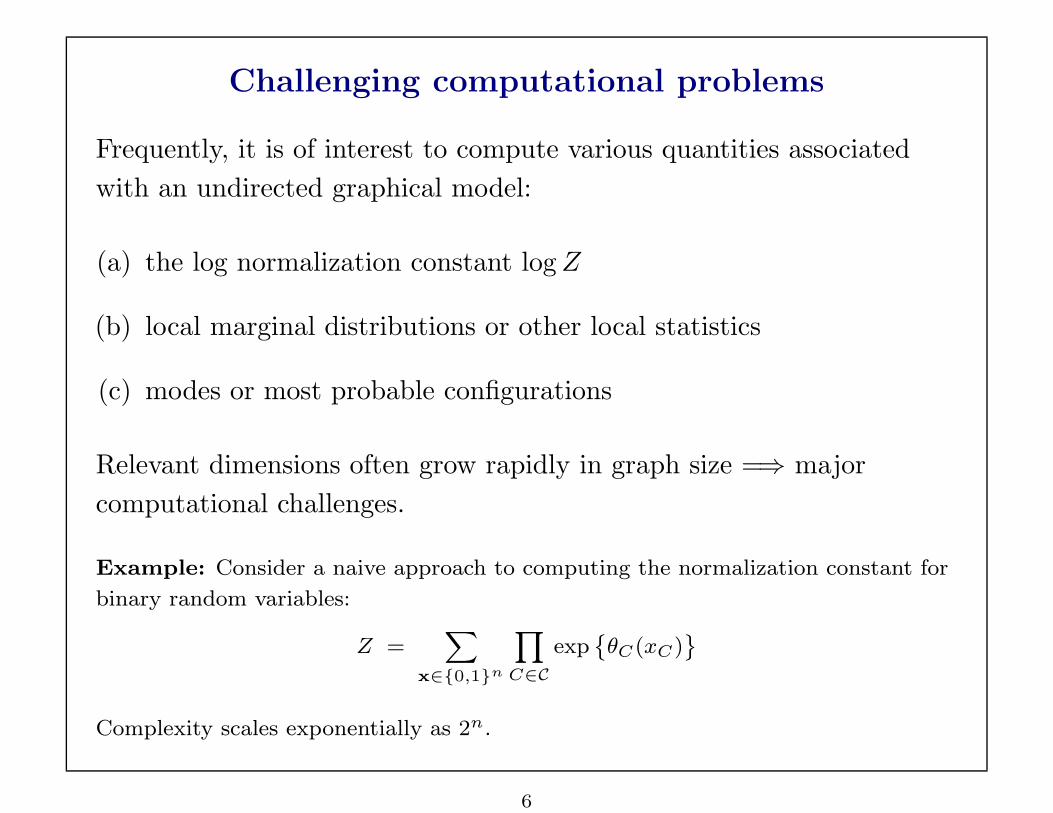
Challenging computational problems
Frequently, it is of interest to compute various quantities associated
with an undirected graphical model:
(a) the log normalization constant log Z
(b) local marginal distributions or other local statistics
(c) modes or most probable configurations
Relevant dimensions often grow rapidly in graph size =⇒ major
computational challenges.
Example: Consider a naive approach to computing the normalization constant for
binary random variables:
Z =X
x∈{0,1}n
Y
C∈C
exp˘
θC(xC)¯
Complexity scales exponentially as 2n.
6
Page 7
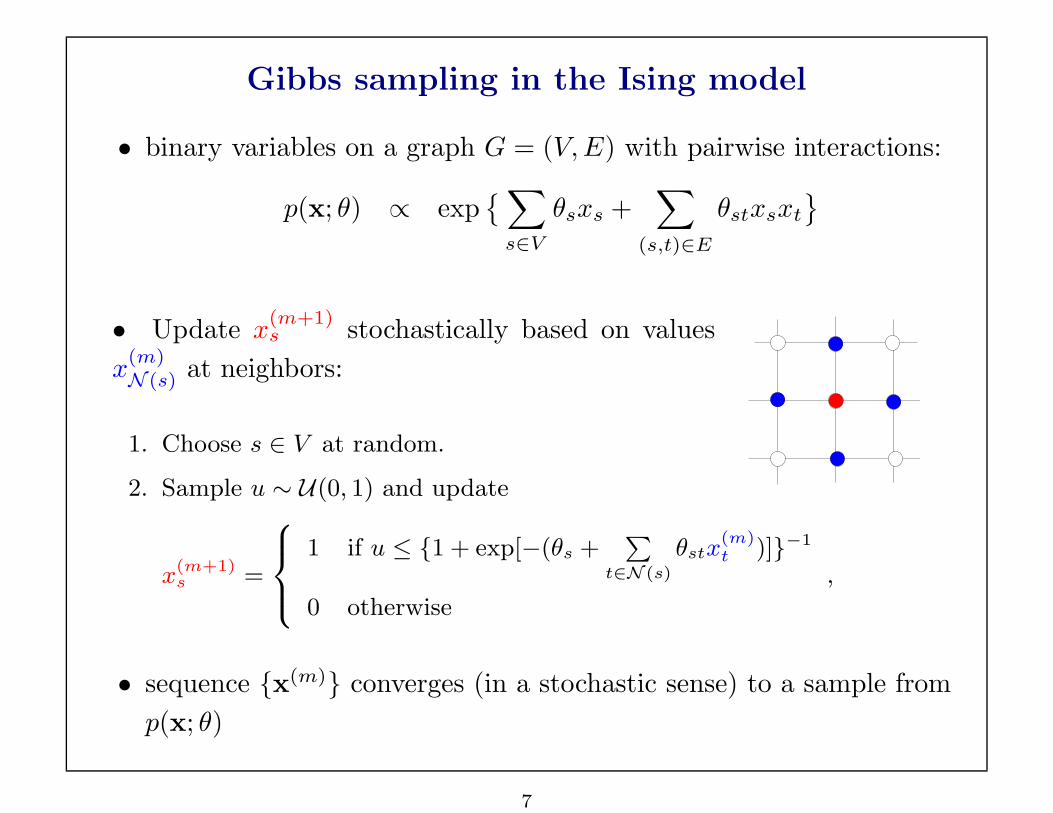
Gibbs sampling in the Ising model
• binary variables on a graph G = (V, E) with pairwise interactions:
p(x; θ) ∝ exp{∑
s∈V
θsxs +∑
(s,t)∈E
θstxsxt
}
• Update x(m+1)s stochastically based on values
x(m)N (s) at neighbors:
1. Choose s ∈ V at random.
2. Sample u ∼ U(0, 1) and update
x(m+1)s =
8><>:
1 if u ≤ {1 + exp[−(θs +P
t∈N (s)
θstx(m)t )]}−1
0 otherwise
,
• sequence {x(m)} converges (in a stochastic sense) to a sample from
p(x; θ)
7
Page 8
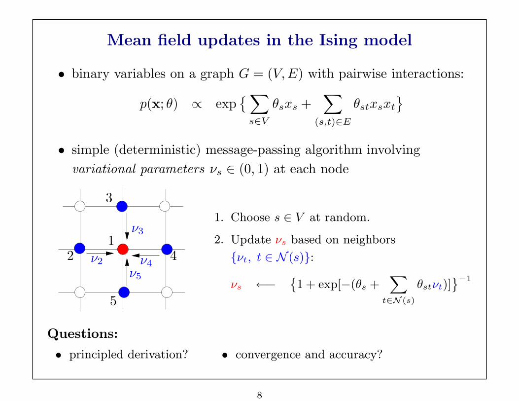
Mean field updates in the Ising model
• binary variables on a graph G = (V, E) with pairwise interactions:
p(x; θ) ∝ exp{∑
s∈V
θsxs +∑
(s,t)∈E
θstxsxt
}
• simple (deterministic) message-passing algorithm involving
variational parameters νs ∈ (0, 1) at each node
PSfrag replacements1
2
3
4
5
ν2
ν3
ν4ν5
1. Choose s ∈ V at random.
2. Update νs based on neighbors
{νt, t ∈ N (s)}:
νs ←−˘1 + exp[−(θs +
X
t∈N (s)
θstνt)]¯−1
Questions:
• principled derivation? • convergence and accuracy?
8
Page 9
Sum and max-product algorithms: On trees
Exact for trees, but approximate for graphs with cycles.
PSfrag replacementsTt
Tu
Tv
Tw
t
w
u
v
s
tMut
Mwt
Mvt
Mts
Mts ≡ message from node t to s
Γ(t) ≡ neighbors of node t
Sum-product: for marginals
(generalizes α− β algorithm; Kalman filter)
Max-product: for MAP configurations
(generalizes Viterbi algorithm)
Update: Mts(xs) ←P
x′
t∈Xt
nexp
hθst(xs, x
′t) + θt(x
′t)i Q
v∈Γ(t)\s
Mvt(xt)o
.
Marginals: p(xs; θ) ∝ exp{θt(xt)}Q
t∈Γ(s) Mts(xs).
9
Page 10
Sum and max-product: On graphs with cycles
• what about applying same updates on graph with cycles?
• updates need not converge (effect of cycles)
• seems naive, but remarkably successful in many applications
PSfrag replacementsTt
Tu
Tv
Tw
t
w
u
v
s
tMut
Mwt
Mvt
Mts
Mts ≡ message from node t to s
Γ(t) ≡ neighbors of node t
Sum-product: for marginals
Max-product: for modes
Questions: • meaning of these updates for graphs with cycles?
• convergence? accuracy of resulting “marginals”?
10
Page 11
Outline1. Recap
(a) Background on graphical models
(b) Some applications and challenging problems
(c) Illustrations of some message-passing algorithms
2. Exponential families and variational methods
(a) What is a variational method (and why should I care)?
(b) Graphical models as exponential families
(c) Variational representations from conjugate duality
3. Exact techniques as variational methods
(a) Gaussian inference on arbitrary graphs
(b) Belief-propagation/sum-product on trees (e.g., Kalman filter; α-β alg.)
(c) Max-product on trees (e.g., Viterbi)
4. Approximate techniques as variational methods
(a) Mean field and variants
(b) Belief propagation and extensions
(c) Convex methods and upper bounds
(d) Tree-reweighted max-product and linear programs
11
Page 12
Variational methods
• “variational”: umbrella term for optimization-based formulation of
problems, and methods for their solution
• historical roots in the calculus of variations
• modern variational methods encompass a wider class of methods
(e.g., dynamic programming; finite-element methods)
Variational principle: Representation of a quantity of interest u as
the solution of an optimization problem.
1. allows the quantity u to be studied through the lens of the
optimization problem
2. approximations to u can be obtained by approximating or relaxing
the variational principle
12
Page 13
Illustration: A simple variational principle
Goal: Given a vector y ∈ Rn and a symmetric matrix Q Â 0, solve the
linear system Qu = y.
Unique solution u(y) = Q−1y can be obtained by matrix inversion.
Variational formulation: Consider the function Jy : Rn → R defined by
Jy(u) :=1
2uT Qu− yT u.
It is strictly convex, and the minimum is uniquely attained:
u(y) = arg minu∈Rn
Jy(u) = Q−1y.
Various methods for solving linear systems (e.g., conjugate gradient)
exploit this variational representation.
13
Page 14
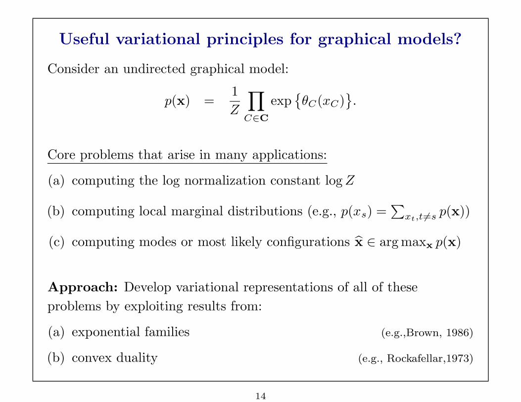
Useful variational principles for graphical models?
Consider an undirected graphical model:
p(x) =1
Z
∏
C∈C
exp{θC(xC)
}.
Core problems that arise in many applications:
(a) computing the log normalization constant log Z
(b) computing local marginal distributions (e.g., p(xs) =∑
xt,t 6=s p(x))
(c) computing modes or most likely configurations x ∈ arg maxx p(x)
Approach: Develop variational representations of all of these
problems by exploiting results from:
(a) exponential families (e.g.,Brown, 1986)
(b) convex duality (e.g., Rockafellar,1973)
14
Page 15
Maximum entropy formulation of graphical models
• suppose that we have measurements µ of the average values of
some (local) functions φα : Xn → R
• in general, will be many distributions p that satisfy the
measurement constraints Ep[φα(x)] = µ
• will consider finding the p with maximum “uncertainty” subject to
the observations, with uncertainty measured by entropy
H(p) = −∑
x
p(x) log p(x).
Constrained maximum entropy problem: Find p to solve
maxp∈P
H(p) such that Ep[φα(x)] = µ
• elementary argument with Lagrange multipliers shows that solution
takes the exponential form
p(x; θ) ∝ exp{∑
α∈I
θαφα(x)}.
15
Page 16
Exponential families
φα : Xn → R ≡ sufficient statistic
φ = {φα, α ∈ I} ≡ vector of sufficient statistics
θ = {θα, α ∈ I} ≡ parameter vector
ν ≡ base measure (e.g., Lebesgue, counting)
• parameterized family of densities (w.r.t. ν):
p(x; θ) = exp{∑
α
θαφα(x) − A(θ)}
• cumulant generating function (log normalization constant):
A(θ) = log( ∫
exp{〈θ, φ(x)〉}ν(dx))
• set of valid parameters Θ := {θ ∈ Rd | A(θ) < +∞}.
• will focus on regular families for which Θ is open.
16
Page 17
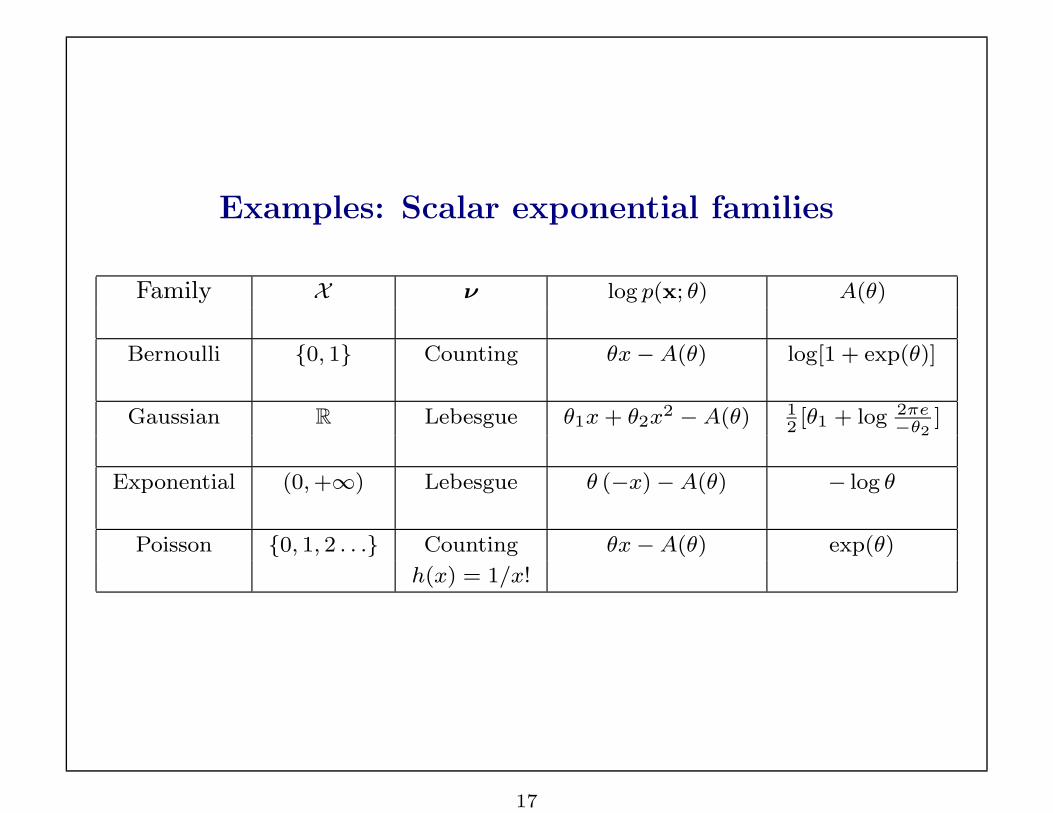
Examples: Scalar exponential families
Family X ν log p(x; θ) A(θ)
Bernoulli {0, 1} Counting θx−A(θ) log[1 + exp(θ)]
Gaussian R Lebesgue θ1x + θ2x2 −A(θ) 12[θ1 + log 2πe
−θ2]
Exponential (0, +∞) Lebesgue θ (−x)−A(θ) − log θ
Poisson {0, 1, 2 . . .} Counting θx−A(θ) exp(θ)
h(x) = 1/x!
17
Page 18
Graphical models as exponential families
• choose random variables Xs at each vertex s ∈ V from an arbitrary
exponential family (e.g., Bernoulli, Gaussian, Dirichlet etc.)
• exponential family can be the same at each node (e.g., multivariate
Gaussian), or different (e.g., mixture models).PSfrag replacements
1
2
3 4
5 6
7
Key requirement: The collection φ of sufficient statistics must
respect the structure of G.
18
Page 19
Example: Discrete Markov random field
PSfrag replacements
θst(xs, xt)θs(xs)θt(xt)
Indicators: I j(xs) =
8
<
:
1 if xs = j
0 otherwise
Parameters: θs = {θs;j , j ∈ Xs}
θst = {θst;jk, (j, k) ∈ Xs ×Xt}
Compact form: θs(xs) :=P
j θs;jI j(xs)
θst(xs, xt) :=P
j,k θst;jkI j(xs)I k(xt)
Density (w.r.t. counting measure) of the form:
p(x; θ) ∝ exp˘X
s∈V
θs(xs) +X
(s,t)∈E
θst(xs, xt)¯
Cumulant generating function (log normalization constant):
A(θ) = logX
x∈Xn
exp˘X
s∈V
θs(xs) +X
(s,t)∈E
θst(xs, xt)¯
19
Page 20
Special case: Hidden Markov model
• Markov chain {X1, X2, . . .} evolving in time, with noisy observation
Yt at each time t
PSfrag replacements
θ23(x2, x3)
θ5(x5)
x1 x2 x3 x4 x5
y1 y2 y3 y4 y5
• an HMM is a particular type of discrete MRF, representing the
conditional p(x |y; θ)
• exponential parameters have a concrete interpretation
θ23(x2, x3) = log p(x3 |x2)
θ5(x5) = log p(y5 |x5)
• the cumulant generating function A(θ) is equal to the log likelihood
log p(y; θ)
20
Page 21
Example: Multivariate Gaussian
U(θ): Matrix of natural parameters φ(x): Matrix of sufficient statistics
2
6
6
6
6
6
6
6
6
6
4
0 θ1 θ2 . . . θn
θ1 θ11 θ12 . . . θ1n
θ2 θ21 θ22 . . . θ2n
......
......
...
θn θn1 θn2 . . . θnn
3
7
7
7
7
7
7
7
7
7
5
2
6
6
6
6
6
6
6
6
6
4
1 x1 x2 . . . xn
x1 (x1)2 x1x2 . . . x1xn
x2 x2x1 (x2)2 . . . x2xn
......
......
...
xn xnx1 xnx2 . . . (xn)2
3
7
7
7
7
7
7
7
7
7
5
Edgewise natural parameters θst = θts must respect graph structure:
1
3
2
4 5
1 2 3 4 5
1
2
3
4
5
(a) Graph structure (b) Structure of [Z(θ)]st = θst.
21
Page 22
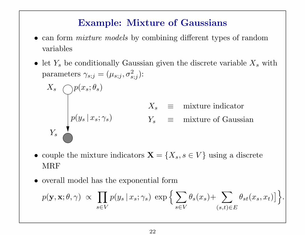
Example: Mixture of Gaussians
• can form mixture models by combining different types of random
variables
• let Ys be conditionally Gaussian given the discrete variable Xs with
parameters γs;j = (µs;j , σ2s;j):
PSfrag replacements
Ys
Xs p(xs; θs)
p(ys |xs; γs)
Xs ≡ mixture indicator
Ys ≡ mixture of Gaussian
• couple the mixture indicators X = {Xs, s ∈ V } using a discrete
MRF
• overall model has the exponential form
p(y,x; θ, γ) ∝∏
s∈V
p(ys |xs; γs) exp{∑
s∈V
θs(xs)+∑
(s,t)∈E
θst(xs, xt)]}
.
22
Page 23
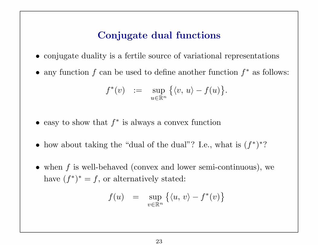
Conjugate dual functions
• conjugate duality is a fertile source of variational representations
• any function f can be used to define another function f ∗ as follows:
f∗(v) := supu∈Rn
{〈v, u〉 − f(u)
}.
• easy to show that f∗ is always a convex function
• how about taking the “dual of the dual”? I.e., what is (f ∗)∗?
• when f is well-behaved (convex and lower semi-continuous), we
have (f∗)∗ = f , or alternatively stated:
f(u) = supv∈Rn
{〈u, v〉 − f∗(v)
}
23
Page 24
Geometric view: Supporting hyperplanes
Question: Given all hyperplanes in Rn × R with normal (v,−1), what
is the intercept of the one that supports epi(f)?
Epigraph of f :
epi(f) := {(u, β) ∈ Rn+1 | f(u) ≤ β}.
PSfrag replacements
f(u)
u(v,−1)
β
−cb
−ca
〈v, u〉 − ca
〈v, u〉 − cb
Analytically, we require the smallest c ∈ R such that:
〈v, u〉 − c ≤ f(u) for all u ∈ Rn
By re-arranging, we find that this optimal c∗ is the dual value:
c∗ = supu∈Rn
˘〈v, u〉 − f(u)
¯.
24
Page 25
Example: Single Bernoulli
Random variable X ∈ {0, 1} yields exponential family of the form:
p(x; θ) ∝ exp˘
θ x¯
with A(θ) = logˆ
1 + exp(θ)˜
.
Let’s compute the dual A∗(µ) := supθ∈R
˘
µθ − log[1 + exp(θ)]¯
.
(Possible) stationary point: µ = exp(θ)/[1 + exp(θ)].
PSfrag replacements
A(θ)
θ
〈µ, θ〉 −A∗(µ)
PSfrag replacements
A(θ)
θ〈µ, θ〉 − c
(a) Epigraph supported (b) Epigraph cannot be supported
We find that: A∗(µ) =
8
<
:
µ log µ + (1− µ) log(1− µ) if µ ∈ [0, 1]
+∞ otherwise..
Leads to the variational representation: A(θ) = maxµ∈[0,1]
˘
µ · θ −A∗(µ)¯
.
25
Page 26
More general computation of the dual A∗
• consider the definition of the dual function:
A∗(µ) = supθ∈Rd
{〈µ, θ〉 −A(θ)
}.
• taking derivatives w.r.t θ to find a stationary point yields:
µ−∇A(θ) = 0.
• Useful fact: Derivatives of A yield mean parameters:
∂A
∂θα
(θ) = Eθ[φα(x)] :=
∫φα(x)p(x; θ)ν(x).
Thus, stationary points satisfy the equation:
µ = Eθ[φ(x)] (1)
26
Page 27
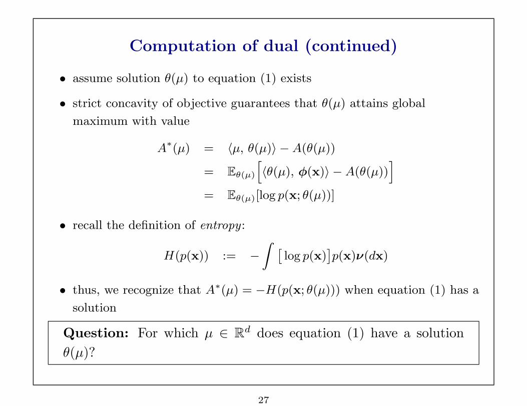
Computation of dual (continued)
• assume solution θ(µ) to equation (1) exists
• strict concavity of objective guarantees that θ(µ) attains global
maximum with value
A∗(µ) = 〈µ, θ(µ)〉 −A(θ(µ))
= Eθ(µ)
h〈θ(µ), φ(x)〉 −A(θ(µ))
i
= Eθ(µ)[log p(x; θ(µ))]
• recall the definition of entropy :
H(p(x)) := −
Z ˆlog p(x)
˜p(x)ν(dx)
• thus, we recognize that A∗(µ) = −H(p(x; θ(µ))) when equation (1) has a
solution
Question: For which µ ∈ Rd does equation (1) have a solution
θ(µ)?
27
Page 28
Sets of realizable mean parameters
• for any distribution p(·), define a vector µ ∈ Rd of mean
parameters:
µα :=
∫φα(x)p(x)ν(dx)
• now consider the setM(G; φ) of all realizable mean
parameters:
M(G; φ) ={µ ∈ R
d∣∣ µα =
∫φα(x)p(x)ν(dx) for some p(·)
}
• for discrete families, we refer to this set as a marginal polytope,
denoted by MARG(G; φ)
28
Page 29
Examples of M: Gaussian MRF
φ(x) Matrix of sufficient statistics U(µ) Matrix of mean parameters
2
6
6
6
6
6
6
6
6
6
4
1 x1 x2 . . . xn
x1 (x1)2 x1x2 . . . x1xn
x2 x2x1 (x2)2 . . . x2xn
......
......
...
xn xnx1 xnx2 . . . (xn)2
3
7
7
7
7
7
7
7
7
7
5
2
6
6
6
6
6
6
6
6
6
4
1 µ1 µ2 . . . µn
µ1 µ11 µ12 . . . µ1n
µ2 µ21 µ22 . . . µ2n
......
......
...
µn µn1 µn2 . . . µnn
3
7
7
7
7
7
7
7
7
7
5
• Gaussian mean parameters are specified by a single semidefinite
constraint as MGauss = {µ ∈ Rn+(n
2) | U(µ) º 0}.
Scalar case:
U(µ) =
24 1 µ1
µ1 µ11
35
PSfrag replacements
Mgauss
µ1
µ11
29
Page 30
Examples of M: Discrete MRF
• sufficient statistics:I j(xs) for s = 1, . . . n, j ∈ Xs
I jk(xs, xt) for(s, t) ∈ E, (j, k) ∈ Xs ×Xt
• mean parameters are simply marginal probabilities, represented as:
µs(xs) :=X
j∈Xs
µs;jI j(xs), µst(xs, xt) :=X
(j,k)∈Xs×Xt
µst;jkI jk(xs, xt)
PSfrag replacements aj
MARG(G)
〈aj , µ〉 = bj
µe • denote the set of realizable µs and µst
by MARG(G)
• refer to it as the marginal polytope
• extremely difficult to characterize for
general graphs
30
Page 31
Geometry and moment mapping
PSfrag replacements
ΘM
θ µ
For suitable classes of graphical models in exponential form, the
gradient map ∇A is a bijection between Θ and the interior ofM.
(e.g., Brown, 1986; Efron, 1978)
31
Page 32
Variational principle in terms of mean parameters
• The conjugate dual of A takes the form:
A∗(µ) =
8<:−H(p(x; θ(µ))) if µ ∈ intM(G;φ)
+∞ if µ /∈ clM(G;φ).
Interpretation:
– A∗(µ) is finite (and equal to a certain negative entropy) for any µ that is
globally realizable
– if µ /∈ clM(G;φ), then the max. entropy problem is infeasible
• The cumulant generating function A has the representation:
A(θ)| {z } = supµ∈M(G;φ)
{〈θ, µ〉 − A∗(µ)}
| {z },
cumulant generating func. max. ent. problem overM
• in contrast to the “free energy” approach, solving this problem provides
both the value A(θ) and the exact mean parameters bµα = Eθ[φα(x)]
32
Page 33
Alternative view: Kullback-Leibler divergence
• Kullback-Leibler divergence defines “distance” between probability
distributions:
D(p || q) :=
Z hlog
p(x)
q(x)
ip(x)ν(dx)
• for two exponential family members p(x; θ1) and p(x; θ2), we have
D(p(x; θ1) || p(x; θ2)) = A(θ2)−A(θ1)− 〈µ1, θ2 − θ1〉
• substituting A(θ1) = 〈θ1, µ1〉 −A∗(µ1) yields a mixed form:
D(p(x; θ1) || p(x; θ2)) ≡ D(µ1 || θ2) = A(θ2) + A∗(µ1)− 〈µ1, θ2〉
Hence, the following two assertions are equivalent:
A(θ2) = supµ1∈M(G;φ)
{〈θ2, µ1〉 − A∗(µ1)}
0 = infµ1∈M(G;φ)
D(µ1 || θ2)
33
Page 34
Challenges
1. In general, mean parameter spaces M can be very difficult to
characterize (e.g., multidimensional moment problems).
2. Entropy A∗(µ) as a function of only the mean parameters µ
typically lacks an explicit form.
Remarks:
1. Variational representation clarifies why certain models are
tractable.
2. For intractable cases, one strategy is to solve an approximate form
of the optimization problem.
34
Page 35
Outline1. Recap
(a) Background on graphical models
(b) Some applications and challenging problems
(c) Illustrations of some message-passing algorithms
2. Exponential families and variational methods
(a) What is a variational method (and why should I care)?
(b) Graphical models as exponential families
(c) Variational representations from conjugate duality
3. Exact techniques as variational methods
(a) Gaussian inference on arbitrary graphs
(b) Belief-propagation/sum-product on trees (e.g., Kalman filter; α-β alg.)
(c) Max-product on trees (e.g., Viterbi)
4. Approximate techniques as variational methods
(a) Mean field and variants
(b) Belief propagation and extensions
(c) Convex methods and upper bounds
(d) Tree-reweighted max-product and linear programs
35
Page 36
A(i): Multivariate Gaussian (fixed covariance)
Consider the set of all Gaussians with fixed inverse covariance Q Â 0.
• potentials φ(x) = {x1, . . . , xn} and natural parameter θ ∈ Θ = Rn.
• cumulant generating function:
density
A(θ) = log
Z
Rn
z }| {
exp˘ nX
s=1
θsxs
¯exp
˘−
1
2x
T Qx¯dx
| {z }base measure
• completing the square yields A(θ) = 12θT Q−1θ + constant
• straightforward computation leads to the dual
A∗(µ) = 12µT Qµ− constant
• putting the pieces back together yields the variational principle
A(θ) = supµ∈Rn
˘θT µ−
1
2µT Qµ
¯+ constant
• optimum is uniquely obtained at the familiar Gaussian mean bµ = Q−1θ.
36
Page 37
A(ii): Multivariate Gaussian (arbitrary covariance)
• matrices of sufficient statistics, natural parameters, and mean
parameters:
φ(x) =
241
x
35h1 x
i, U(θ) :=
24 0 [θs]
[θs] [θst]
35 U(µ) := E
(241
x
35h1 x
i)
• cumulant generating function:
A(θ) = log
Zexp
n〈〈U(θ), φ(x)〉〉
odx
• computing the dual function:
A∗(µ) = −1
2log det U(µ)−
n
2log 2πe,
• exact variational principle is a log-determinant problem:
A(θ) = supU(µ)Â0, [U(µ)]11=1
˘〈〈U(θ), U(µ)〉〉+
1
2log det U(µ)
¯+
n
2log 2πe
• solution yields the normal equations for Gaussian mean and covariance.
37
Page 38
B: Belief propagation/sum-product on trees
• discrete variables Xs ∈ {0, 1, . . . , ms − 1} on a tree T = (V, E)
• sufficient statistics: indicator functions for each node and edge
I j(xs) for s = 1, . . . n, j ∈ Xs
I jk(xs, xt) for (s, t) ∈ E, (j, k) ∈ Xs ×Xt.
• exponential representation of distribution:
p(x; θ) ∝ exp˘X
s∈V
θs(xs) +X
(s,t)∈E
θst(xs, xt)¯
where θs(xs) :=P
j∈Xsθs;jI j(xs) (and similarly for θst(xs, xt))
• mean parameters are simply marginal probabilities, represented as:
µs(xs) :=X
j∈Xs
µs;jI j(xs), µst(xs, xt) :=X
(j,k)∈Xs×Xt
µst;jkI jk(xs, xt)
• the marginals must belong to the following marginal polytope:
MARG(T ) := { µ ≥ 0 |X
xs
µs(xs) = 1,X
xt
µst(xs, xt) = µs(xs) },
38
Page 39
Decomposition of entropy for trees
• by the junction tree theorem, any tree can be factorized in terms of
its marginals µ ≡ µ(θ) as follows:
p(x; θ) =∏
s∈V
µs(xs)∏
(s,t)∈E
µst(xs, xt)
µs(xs)µt(xt)
• taking logs and expectations leads to an entropy decomposition
H(p(x; θ)) = −A∗(µ(θ)) =∑
s∈V
Hs(µs)−∑
(s,t)∈E
Ist(µst)
where
Single node entropy: Hs(µs) := −∑
xsµs(xs) log µs(xs)
Mutual information: Ist(µst) :=∑
xs,xtµst(xs, xt) log µst(xs,xt)
µs(xs)µt(xt).
• thus, the dual function A∗(µ) has an explicit and easy form
39
Page 40
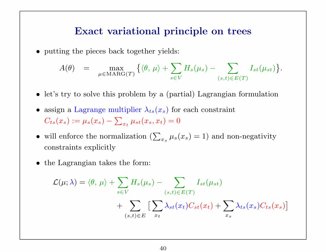
Exact variational principle on trees
• putting the pieces back together yields:
A(θ) = maxµ∈MARG(T )
˘〈θ, µ〉+
X
s∈V
Hs(µs)−X
(s,t)∈E(T )
Ist(µst)¯.
• let’s try to solve this problem by a (partial) Lagrangian formulation
• assign a Lagrange multiplier λts(xs) for each constraint
Cts(xs) := µs(xs)−P
xtµst(xs, xt) = 0
• will enforce the normalization (P
xsµs(xs) = 1) and non-negativity
constraints explicitly
• the Lagrangian takes the form:
L(µ; λ) = 〈θ, µ〉+X
s∈V
Hs(µs)−X
(s,t)∈E(T )
Ist(µst)
+X
(s,t)∈E
ˆX
xt
λst(xt)Cst(xt) +X
xs
λts(xs)Cts(xs)˜
40
Page 41
Lagrangian derivation (continued)
• taking derivatives of the Lagrangian w.r.t µs and µst yields
∂L
∂µs(xs)= θs(xs)− log µs(xs) +
X
t∈N (s)
λts(xs) + C
∂L
∂µst(xs, xt)= θst(xs, xt)− log
µst(xs, xt)
µs(xs)µt(xt)− λts(xs)− λst(xt) + C ′
• setting these partial derivatives to zero and simplifying:
µs(xs) ∝ exp˘
θs(xs)¯
Y
t∈N (s)
exp˘
λts(xs)¯
µs(xs, xt) ∝ exp˘
θs(xs) + θt(xt) + θst(xs, xt)¯
×Y
u∈N (s)\t
exp˘
λus(xs)¯
Y
v∈N (t)\s
exp˘
λvt(xt)¯
• enforcing the constraint Cts(xs) = 0 on these representations yields thefamiliar update rule for the messages Mts(xs) = exp(λts(xs)):
Mts(xs) ←X
xt
exp˘
θt(xt) + θst(xs, xt)¯
Y
u∈N (t)\s
Mut(xt)
41
Page 42
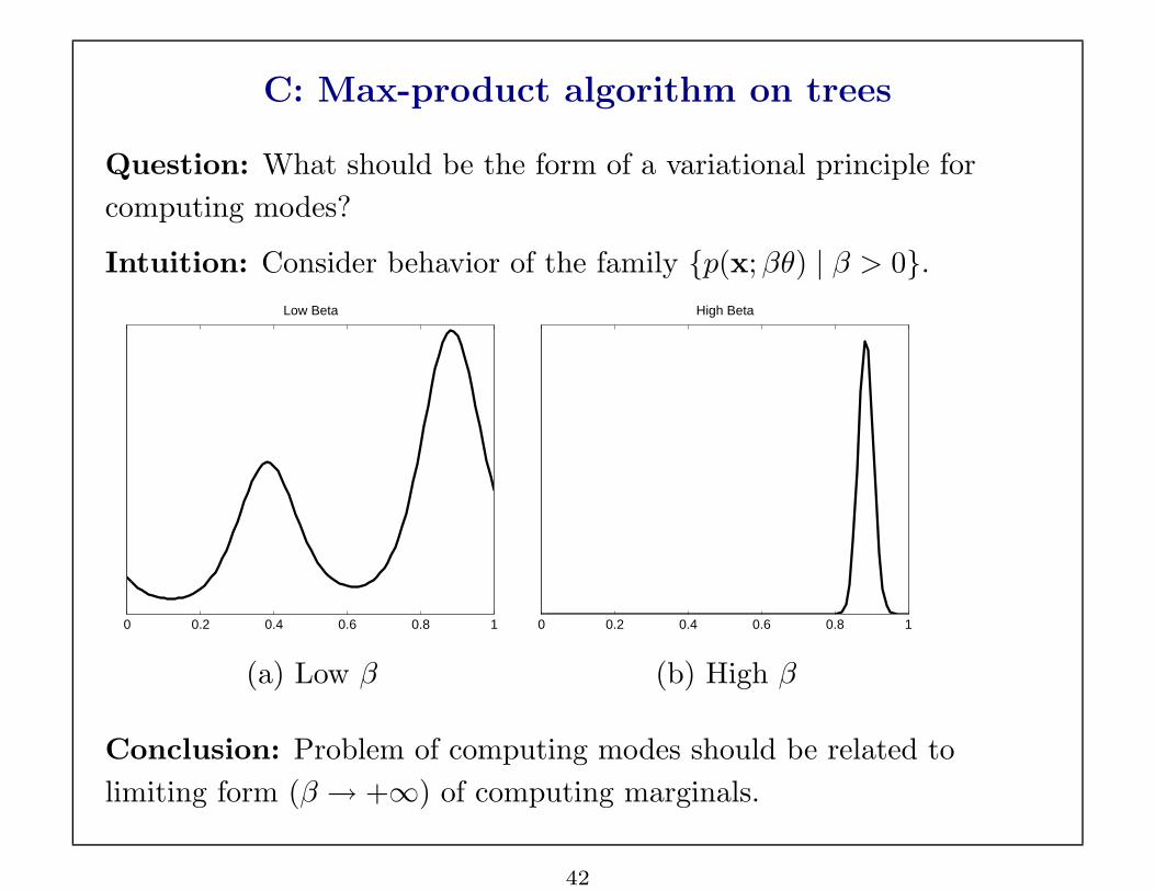
C: Max-product algorithm on trees
Question: What should be the form of a variational principle for
computing modes?
Intuition: Consider behavior of the family {p(x; βθ) | β > 0}.
0 0.2 0.4 0.6 0.8 1
Low Beta
0 0.2 0.4 0.6 0.8 1
High Beta
(a) Low β (b) High β
Conclusion: Problem of computing modes should be related to
limiting form (β → +∞) of computing marginals.
42
Page 43
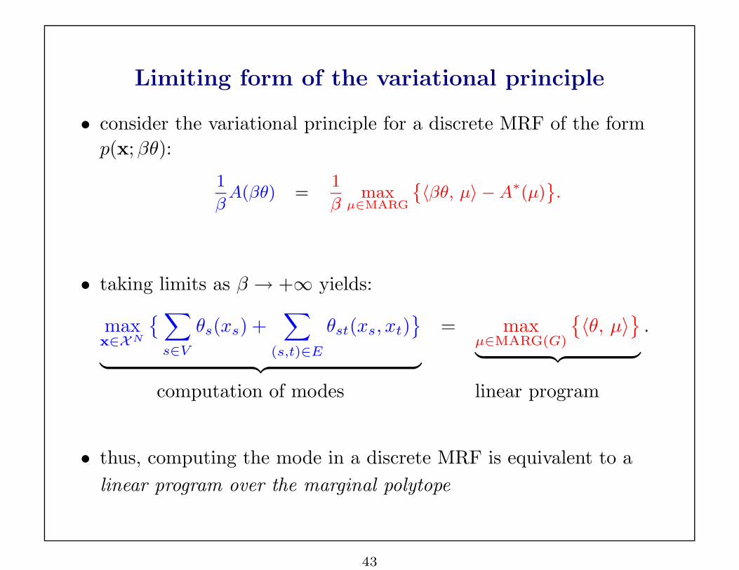
Limiting form of the variational principle
• consider the variational principle for a discrete MRF of the form
p(x; βθ):
1
βA(βθ) =
1
βmax
µ∈MARG
˘〈βθ, µ〉 −A∗(µ)
¯.
• taking limits as β → +∞ yields:
maxx∈XN
{∑
s∈V
θs(xs) +∑
(s,t)∈E
θst(xs, xt)}
︸ ︷︷ ︸
= maxµ∈MARG(G)
{〈θ, µ〉
}
︸ ︷︷ ︸.
computation of modes linear program
• thus, computing the mode in a discrete MRF is equivalent to a
linear program over the marginal polytope
43
Page 44
Max-product on tree-structured MRFs
• recall the max-product (belief revision) updates:
Mts(xs) ← maxxt
exp{θt(xt) + θst(xs, xt)
} ∏
u∈N (t)\s
Mut(xt)
• for trees, the variational principle (linear program) takes the
especially simple form
maxµ∈MARG(T )
{∑
s∈V
θs(xs)µs(xs) +∑
(s,t)∈E
θst(xs, xt)µst(xs, xt)}
• constraint set is the marginal polytope for trees
MARG(T ) := { µ ≥ 0 |∑
xs
µs(xs) = 1,∑
xt
µst(xs, xt) = µs(xs) },
• a similar Lagrangian formulation shows that max-product is an
iterative method for solving this linear program (details in Wainwright
& Jordan, 2003)
44
Page 45
Outline1. Recap
(a) Background on graphical models
(b) Some applications and challenging problems
(c) Illustrations of some message-passing algorithms
2. Exponential families and variational methods
(a) What is a variational method (and why should I care)?
(b) Graphical models as exponential families
(c) Variational representations from conjugate duality
3. Exact techniques as variational methods
(a) Gaussian inference on arbitrary graphs
(b) Belief-propagation/sum-product on trees (e.g., Kalman filter; α-β alg.)
(c) Max-product on trees (e.g., Viterbi)
4. Approximate techniques as variational methods
(a) Mean field and variants
(b) Belief propagation and extensions
(c) Convex relaxations and upper bounds
(d) Tree-reweighted max-product and linear programs
45
Page 46
A: Mean field theory
Difficulty: (typically) no explicit form for −A∗(µ) (i.e., entropy as a
function of mean parameters) =⇒ exact variational principle is
intractable.
Idea: Restrict µ to a subset of distributions for which −A∗(µ) has a
tractable form.
Examples:
(a) For product distributions p(x) =∏
s∈V µs(xs), entropy decomposes
as −A∗(µ) =∑
s∈V Hs(xs).
(b) Similarly, for trees (more generally, decomposable graphs), the
junction tree theorem yields an explicit form for −A∗(µ).
Definition: A subgraph H of G is tractable if the entropy has an
explicit form for any distribution that respects H.
46
Page 47
Geometry of mean field
• let H represent a tractable subgraph (i.e., for which
A∗ has explicit form)
• letMtr(G; H) represent tractable mean parameters:
Mtr(G; H) := {µ| µ = Eθ[φ(x)] s. t. θ respects H}.
1 2
65
9
3
4
7 8
1 2
65
9
3
4
7 8
PSfrag replacements
µe
M
Mtr• under mild conditions, Mtr is a non-
convex inner approximation to M
• optimizing overMtr (as opposed toM)
yields lower bound :
A(θ) ≥ supeµ∈Mtr
˘〈θ, eµ〉 −A∗(eµ)
¯.
47
Page 48
Alternative view: Minimizing KL divergence
• recall the mixed form of the KL divergence between p(x; θ) and
p(x; θ):
D(µ || θ) = A(θ) + A∗(µ)− 〈µ, θ〉
• try to find the “best” approximation to p(x; θ) in the sense of KL
divergence
• in analytical terms, the problem of interest is
infeµ∈Mtr
D(µ || θ) = A(θ) + infeµ∈Mtr
{A∗(µ)− 〈µ, θ〉
}
• hence, finding the tightest lower bound on A(θ) is equivalent to
finding the best approximation to p(x; θ) from distributions with
µ ∈Mtr
48
Page 49
Example: Naive mean field algorithm for Ising model
• consider completely disconnected subgraph H = (V, ∅)
• permissible exponential parameters belong to subspace
E(H) = {θ ∈ Rd | θst = 0 ∀ (s, t) ∈ E}
• allowed distributions take product form p(x; θ) =∏
s∈V
p(xs; θs), and
generate
Mtr(G; H) = {µ | µst = µsµt, µs ∈ [0, 1] }.
• approximate variational principle:
maxµs∈[0,1]
X
s∈V
θsµs+X
(s,t)∈E
θstµsµt−ˆ
X
s∈V
µs log µs+(1−µs) log(1−µs)˜
ff
.
• Co-ordinate ascent: with all {µt, t 6= s} fixed, problem is strictly
concave in µs and optimum is attained at
µs ←−{1 + exp[−(θs +
∑
t∈N (s)
θstµt)]}−1
49
Page 50
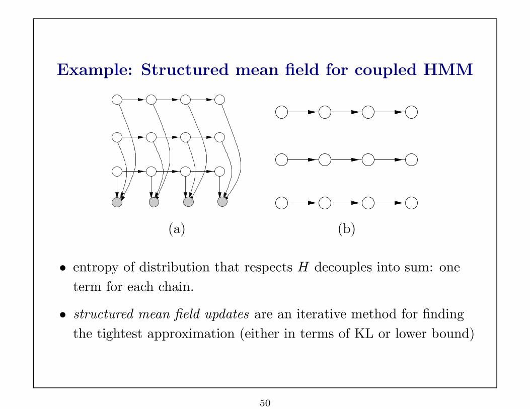
Example: Structured mean field for coupled HMM
(a) (b)
• entropy of distribution that respects H decouples into sum: one
term for each chain.
• structured mean field updates are an iterative method for finding
the tightest approximation (either in terms of KL or lower bound)
50
Page 51
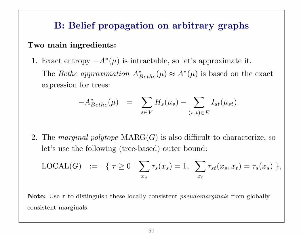
B: Belief propagation on arbitrary graphs
Two main ingredients:
1. Exact entropy −A∗(µ) is intractable, so let’s approximate it.
The Bethe approximation A∗Bethe(µ) ≈ A∗(µ) is based on the exact
expression for trees:
−A∗Bethe(µ) =
∑
s∈V
Hs(µs)−∑
(s,t)∈E
Ist(µst).
2. The marginal polytope MARG(G) is also difficult to characterize, so
let’s use the following (tree-based) outer bound:
LOCAL(G) := { τ ≥ 0 |∑
xs
τs(xs) = 1,∑
xt
τst(xs, xt) = τs(xs) },
Note: Use τ to distinguish these locally consistent pseudomarginals from globally
consistent marginals.
51
Page 52
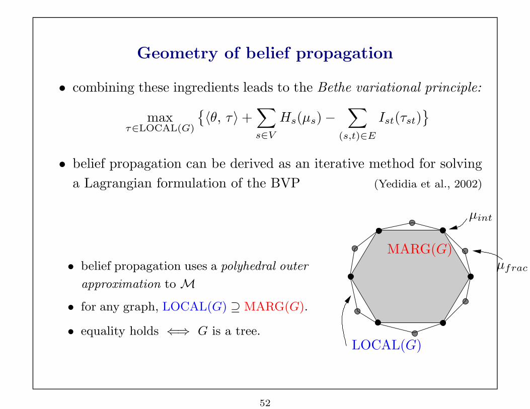
Geometry of belief propagation
• combining these ingredients leads to the Bethe variational principle:
maxτ∈LOCAL(G)
{〈θ, τ〉+
∑
s∈V
Hs(µs)−∑
(s,t)∈E
Ist(τst)}
• belief propagation can be derived as an iterative method for solving
a Lagrangian formulation of the BVP (Yedidia et al., 2002)
• belief propagation uses a polyhedral outer
approximation toM
• for any graph, LOCAL(G) ⊇ MARG(G).
• equality holds ⇐⇒ G is a tree.
PSfrag replacements
µint
LOCAL(G)
MARG(G)µfrac
52
Page 53
Illustration: Globally inconsistent BP fixed points
Consider the following assignment of pseudomarginals τs, τst:
Locally consistent
(pseudo)marginals
3
2
1
�� �� � ��
� �� � � � �
�� �� � ��
� � � � ���
�� � �
� � � ��� � �
� � � �
�� � �
� � � ��
� �� � � �
� �� � ���
• can verify that τ ∈ LOCAL(G), and that τ is a fixed point of belief
propagation (with all constant messages)
• however, τ is globally inconsistent
Note: More generally: for any τ in the interior of LOCAL(G), can
construct a distribution with τ as a BP fixed point.
53
Page 54
High-level perspective
• message-passing algorithms (e.g., mean field, belief propagation)
are solving approximate versions of exact variational principle in
exponential families
• there are two distinct components to approximations:
(a) can use either inner or outer bounds toM
(b) various approximations to entropy function −A∗(µ)
• mean field: non-convex inner bound and exact form of entropy
• BP: polyhedral outer bound and non-convex Bethe approximation
• Kikuchi and variants: tighter polyhedral outer bounds and better
entropy approximations
(e.g.,Yedidia et al., 2002)
54
Page 55
Generalized belief propagation on hypergraphs
• a hypergraph is a natural generalization of a graph
• it consists of a set of vertices V and a set E of hyperedges, where
each hyperedge is a subset of V
• convenient graphical representation in terms of poset diagrams
1 2
3 4
14
1 2
2
4 3
31 2 3 2 3 4
2 3
1 2 4 552
2 3 5 6
5
54 7 85 8
5 6 8 9
4 5 5 6
(a) Ordinary graph (b) Hypertree (width 2) (c) Hypergraph
• descendants and ancestors of a hyperedge h:
D+(h) := {g ∈ E | g ⊆ h }, A+(h) := {g ∈ E | g ⊇ h }.
55
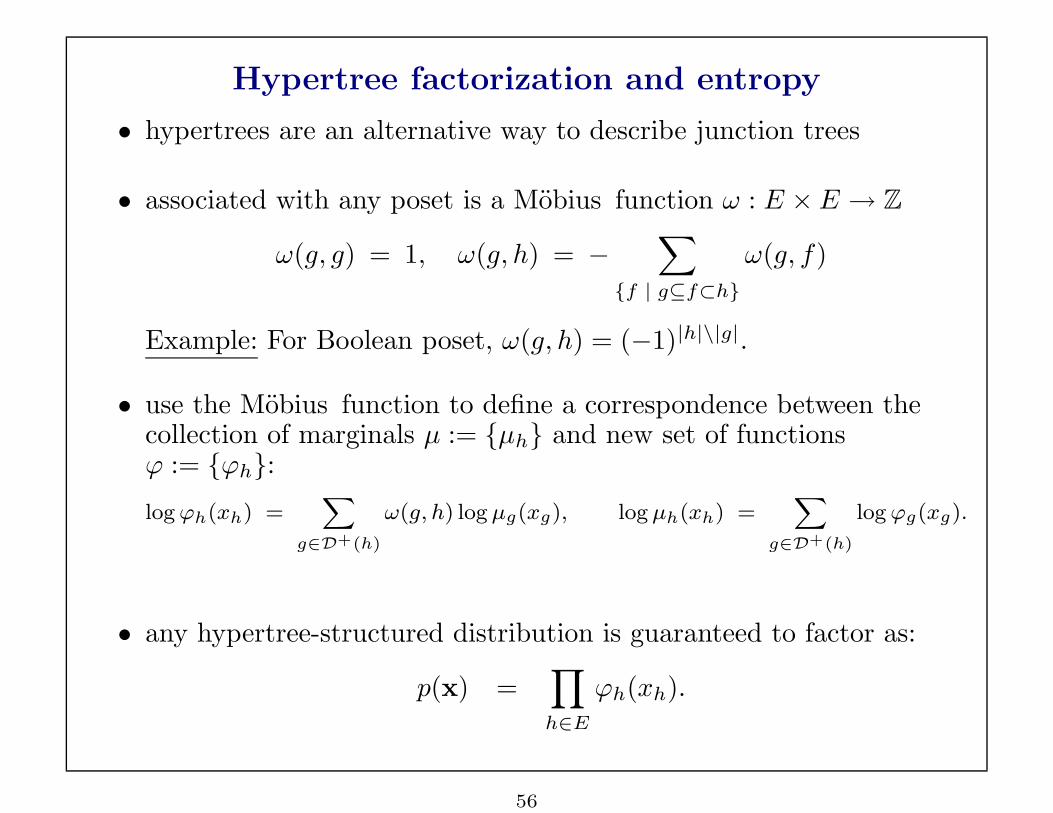
Page 56
Hypertree factorization and entropy
• hypertrees are an alternative way to describe junction trees
• associated with any poset is a Mobius function ω : E × E → Z
ω(g, g) = 1, ω(g, h) = −∑
{f | g⊆f⊂h}
ω(g, f)
Example: For Boolean poset, ω(g, h) = (−1)|h|\|g|.
• use the Mobius function to define a correspondence between thecollection of marginals µ := {µh} and new set of functionsϕ := {ϕh}:
log ϕh(xh) =X
g∈D+(h)
ω(g, h) log µg(xg), log µh(xh) =X
g∈D+(h)
log ϕg(xg).
• any hypertree-structured distribution is guaranteed to factor as:
p(x) =∏
h∈E
ϕh(xh).
56
Page 57
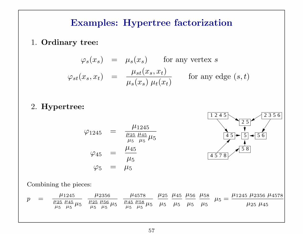
Examples: Hypertree factorization
1. Ordinary tree:
ϕs(xs) = µs(xs) for any vertex s
ϕst(xs, xt) =µst(xs, xt)
µs(xs) µt(xt)for any edge (s, t)
2. Hypertree:
ϕ1245 =µ1245
µ25
µ5
µ45
µ5µ5
ϕ45 =µ45
µ5
ϕ5 = µ5
1 2 4 552
2 3 5 6
54 5 5 6
54 7 85 8
Combining the pieces:
p =µ1245
µ25
µ5
µ45
µ5µ5
µ2356µ25
µ5
µ56
µ5µ5
µ4578µ45
µ5
µ58
µ5µ5
µ25
µ5
µ45
µ5
µ56
µ5
µ58
µ5µ5 =
µ1245 µ2356 µ4578
µ25 µ45
57
Page 58
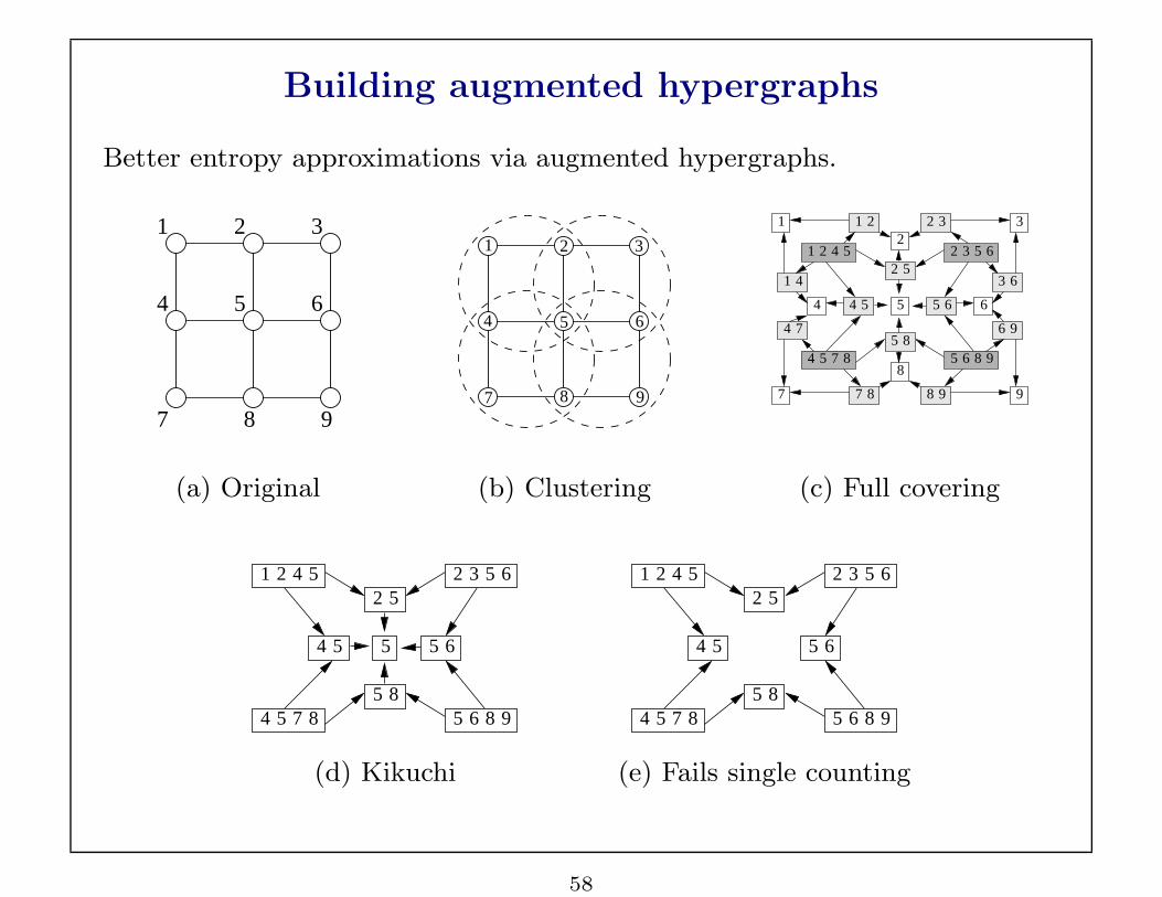
Building augmented hypergraphs
Better entropy approximations via augmented hypergraphs.
1 2
65
9
3
4
7 8
1 2
87
4
3
9
5 6
1 2 4 5
54 7 8 5 6 8 9
2 3 5 6
7 8 8 9
5 6
4 7
1 4
4 5
1 2 2 3
6 9
8
4 5
5 8
52
2
3 6
6
1
7
3
9
(a) Original (b) Clustering (c) Full covering
1 2 4 552
2 3 5 6
5
54 7 85 8
5 6 8 9
4 5 5 6
1 2 4 552
2 3 5 6
54 7 85 8
5 6 8 9
4 5 5 6
(d) Kikuchi (e) Fails single counting
58
Page 59
C. Convex relaxations and upper bounds
Possible concerns with the Bethe/Kikuchi problems and variations?
(a) lack of convexity ⇒ multiple local optima, and substantial
algorithmic complications
(b) failure to bound the log partition function
Goal: Techniques for approximate computation of marginals and
parameter estimation based on:
(a) convex variational problems ⇒ unique global optimum
(b) relaxations of exact problem ⇒ upper bounds on A(θ)
Usefulness of bounds:
(a) interval estimates for marginals
(b) approximate parameter estimation
(c) large deviations (prob. of rare events)
59
Page 60
Bounds from “convexified” Bethe/Kikuchi problems
Idea: Upper bound −A∗(µ) by convex combination of tree-structured
entropies.
PSfrag replacementsPSfrag replacements PSfrag replacements PSfrag replacements
−A∗(µ) ≤ −ρ(T 1)A∗(µ(T 1)) − ρ(T 2)A∗(µ(T 2)) − ρ(T 3)A∗(µ(T 3))
• given any spanning tree T , define the moment-matched tree distribution:
p(x; µ(T )) :=Y
s∈V
µs(xs)Y
(s,t)∈E
µst(xs, xt)
µs(xs) µt(xt)
• use −A∗(µ(T )) to denote the associated tree entropy
• let ρ = {ρ(T )} be a probability distribution over spanning trees
60
Page 61
Edge appearance probabilities
Experiment: What is the probability ρe that a given edge e ∈ E
belongs to a tree T drawn randomly under ρ?
PSfrag replacements
e
b
f
PSfrag replacements
e
b
f
PSfrag replacements
e
b
f
PSfrag replacements
e
b
f
(a) Original (b) ρ(T 1) = 13
(c) ρ(T 2) = 13
(d) ρ(T 3) = 13
In this example: ρb = 1; ρe = 23 ; ρf = 1
3 .
The vector ρe = { ρe | e ∈ E } must belong to the spanning tree
polytope, denoted T(G). (Edmonds, 1971)
61
Page 62
Optimal bounds by tree-reweighted message-passing
Recall the constraint set of locally consistent marginal distributions:
LOCAL(G) = { τ ≥ 0 |X
xs
τs(xs) = 1,
| {z }
X
xs
τst(xs, xt) = τt(xt)
| {z }}.
normalization marginalization
Theorem: (Wainwright, Jaakkola, & Willsky, 2002; To appear in IEEE-IT)
(a) For any given edge weights ρe = {ρe} in the spanning tree polytope,
the optimal upper bound over all tree parameters is given by:
A(θ) ≤ maxτ∈LOCAL(G)
˘〈θ, τ〉+
X
s∈V
Hs(τs)−X
(s,t)∈E
ρstIst(τst)¯.
(b) This optimization problem is strictly convex, and its unique optimum
is specified by the fixed point of ρe-reweighted message passing:
M∗ts(xs) = κ
X
x′
t∈Xt
(exp
hθst(xs, x′t)
ρst
+ θt(x′t)i
Qv∈Γ(t)\s
ˆM∗
vt(xt)˜ρvt
ˆM∗
st(xt)˜(1−ρts)
).
62
Page 63
Semidefinite constraints in convex relaxations
Fact: Belief propagation and its hypergraph-based generalizations all
involve polyhedral (i.e., linear) outer bounds on the marginal polytope.
Idea: Use semidefinite constraints to generate more global outer
bounds.
Example: For the Ising model, relevant mean parameters are µs = p(Xs = 1) and
µst = p(Xs = 1, Xt = 1).
Define y = [1 x]T , and consider the second-order moment matrix:
E[yyT ] =
2
6
6
6
6
6
6
6
6
6
4
1 µ1 µ2 . . . µn
µ1 µ1 µ12 . . . µ1n
µ2 µ12 µ2 . . . µ2n
......
......
...
µn µn1 µn2 . . . µn
3
7
7
7
7
7
7
7
7
7
5
It must be positive semidefinite, which imposes (an infinite number of) linear
constraints on µs, µst.
63
Page 64
Illustrative example
Locally consistent
(pseudo)marginals
3
2
1
�� �� � ��
� �� � � � �
�� �� � ��
� � � � ���
�� � �
� � � ��� � �
� � � �
�� � �
� � � ��
� �� � � �
� �� � ���
Second-order
moment matrix
µ1 µ12 µ13
µ21 µ2 µ23
µ31 µ32 µ3
=
0.5 0.4 0.1
0.4 0.5 0.4
0.1 0.4 0.5
Not positive-semidefinite!
64
Page 65
Log-determinant relaxation
• based on optimizing over covariance matrices M1(µ) ∈ SDEF1(Kn)
Theorem: Consider an outer bound OUT(Kn) that satisfies:
MARG(Kn) ⊆ OUT(Kn) ⊆ SDEF1(Kn)
For any such outer bound, A(θ) is upper bounded by:
maxµ∈OUT(Kn)
{〈θ, µ〉+
1
2log det
[M1(µ)+
1
3blkdiag[0, In]
]}+
n
2log(
πe
2)
Remarks:
1. Log-det. problem can be solved efficiently by interior point methods.
2. Relevance for applications:
(a) Upper bound on A(θ).
(b) Method for computing approximate marginals.
(Wainwright & Jordan, 2003)
65
Page 66
Results for approximating marginals
0 0.1 0.2 0.3 0.4 0.5 0.6 0.7 0.8
Strong +
Weak +
Strong +/−
Weak +/−
Strong −
Weak −
Nearest−neighbor grid
Average error in marginal
LDBP
0 0.1 0.2 0.3 0.4 0.5 0.6 0.7 0.8
Strong +
Weak +
Strong +/−
Weak +/−
Strong −
Weak −
Fully connected
Average error in marginal
LDBP
(a) Nearest-neighbor grid (b) Fully connected
• average `1 error in approximate marginals over 100 trials
• coupling types: repulsive (−), mixed (+/−), attractive (+)
66
Page 67
D. Tree-reweighted max-product algorithm
• integer program (IP): optimizing cost function over a discrete space
(e.g., {0, 1}n)
• IPs computationally intractable in general, but graphical structure
can be exploited
• tree-structured IPs solvable in linear time with dynamic
programming (max-product message-passing)
• standard max-product algorithm applied to graphs with cycles, but
no guarantees in general
• a novel perspective:
– “tree-reweighted” max-product for arbitrary graphs
– optimality guarantees for reweighted message-passing
– forges connection between max-product message passing and linear
programming (LP) relaxations
67
Page 68
Some previous theory on ordinary max-product
• analysis of single-cycle graphs (Aji & McEliece, 1998; Horn, 1999; Weiss,
1998)
• guarantees for attenuated max-product updates (Frey & Koetter, 2001)
• locally optimal on “tree-plus-loop” neighborhoods (Weiss & Freeman,
2001)
• strengthened optimality results and computable error bounds on
the gap (Wainwright et al., 2003)
• exactness after finite # iterations for max. weight bipartite
matching (Bayati, Shah & Sharma, 2005)
68
Page 69
Standard analysis via computation tree
• standard tool: computation tree of message-passing updates
(Gallager, 1963; Weiss, 2001; Richardson & Urbanke, 2001)
PSfrag replacements
1
2 3
4
PSfrag replacements
11
11
1
222
2
2
2
3 33
3
3
3
44
4 4
(a) Original graph (b) Computation tree (4 iterations)
• level t of tree: all nodes whose messages reach the root (node 1)
after t iterations of message-passing
69
Page 70
Illustration: Non-exactness of standard max-product
Intuition:
• max-product is solving (exactly) a modified problem on the computation
tree
• nodes not equally weighted in computation tree ⇒ max-product can
output an incorrect configuration
PSfrag replacements
1
2 3
4
PSfrag replacements
11
11
1
222
2
2
2
3 33
3
3
3
44
4 4
(a) Diamond graph Gdia (b) Computation tree (4 iterations)
• for example: asymptotic node fractions in this computation tree:hf(1) f(2) f(3) f(4)
i=
h0.2393 0.2607 0.2607 0.2393
i
70
Page 71
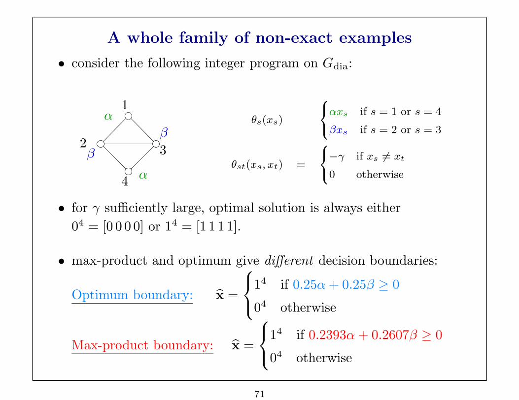
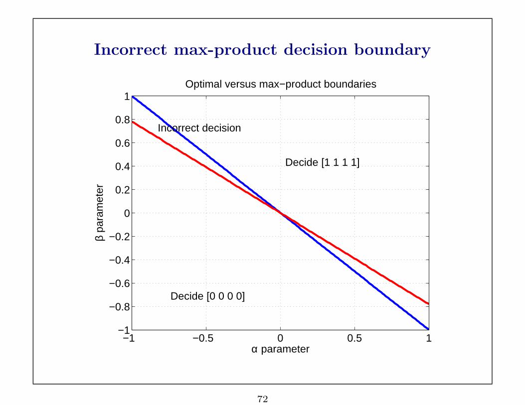
A whole family of non-exact examples
• consider the following integer program on Gdia:
PSfrag replacements
1
23
4
α
α
β
β
θs(xs)
8
<
:
αxs if s = 1 or s = 4
βxs if s = 2 or s = 3
θst(xs, xt) =
8
<
:
−γ if xs 6= xt
0 otherwise
• for γ sufficiently large, optimal solution is always either
04 = [0 0 0 0] or 14 = [1 1 1 1].
• max-product and optimum give different decision boundaries:
Optimum boundary: x =
14 if 0.25α + 0.25β ≥ 0
04 otherwise
Max-product boundary: x =
14 if 0.2393α + 0.2607β ≥ 0
04 otherwise
71
Page 72
Incorrect max-product decision boundary
−1 −0.5 0 0.5 1−1
−0.8
−0.6
−0.4
−0.2
0
0.2
0.4
0.6
0.8
1
α parameter
β pa
ram
eter
Optimal versus max−product boundaries
Decide [1 1 1 1]
Decide [0 0 0 0]
Incorrect decision
72
Page 73
Tree-reweighted max-product algorithm
(Wainwright, Jaakkola & Willsky, 2002)
Message update from node t to node s:
reweighted messages
Mts(xs) ← κ maxx′
t∈Xt
(exp
hθst(xs, x′t)
ρst| {z }+ θt(x
′t)i
Qv∈Γ(t)\s
z }| {ˆMvt(xt)
˜ρvt
ˆMst(xt)
˜(1−ρts)
| {z }
).
reweighted edge opposite message
Properties:
1. Modified updates remain distributed and purely local over the graph.
2. Key differences:
• Messages are reweighted with ρst ∈ [0, 1].
• Potential on edge (s, t) is rescaled by ρst ∈ [0, 1].
• Update involves the reverse direction edge.
3. The choice ρst = 1 for all edges (s, t) recovers standard update.
73
Page 74
TRW max-product computes pseudo-max-marginals
• observe that the mode-finding problem can be solved via the exact
max-marginals:
µs(xs) := max{x′ | x′
s=xs}
p(x′), µst(xs, xt) := max{x′ | x′
s=xs,x′
t=xt}
p(x′)
• any message fixed point M∗ defines a set of pseudo-max-marginals
{ν∗s , ν∗
st} at nodes and edges
• will show these TRW message-passing never “lies”, and establish
optimality guarantees for suitable fixed points
• guarantees require the following conditions:
(a) Weight choice: the edge weights ρ = {ρst | (s, t) ∈ E} are
“suitably” chosen (in the spanning tree polytope)
(b) Strong tree agreement: There exists an x∗ such that:
– Nodewise optimal: x∗s belongs to arg maxxs
ν∗s (xs).
– Edgewise optimal: (x∗s , x∗
t ) belongs to arg maxxs,xtν∗
st(xs, xt).
74
Page 75
Edge appearance probabilities
Experiment: What is the probability ρe that a given edge e ∈ E
belongs to a tree T drawn randomly under ρ?
PSfrag replacements
e
b
f
PSfrag replacements
e
b
f
PSfrag replacements
e
b
f
PSfrag replacements
e
b
f
(a) Original (b) ρ(T 1) = 13
(c) ρ(T 2) = 13
(d) ρ(T 3) = 13
In this example: ρb = 1; ρe = 23 ; ρf = 1
3 .
The vector ρe = { ρe | e ∈ E } must belong to the spanning tree
polytope, denoted T(G). (Edmonds, 1971)
75
Page 76
TRW max-product never “lies”
Set-up: Any fixed point ν∗ that satisfies the strong tree agreement
(STA) condition defines a configuration x∗ = (x∗1, . . . , x
∗n) such that
x∗s ∈ arg max
xs
ν∗s (xs),
︸ ︷︷ ︸(x∗
s, x∗t ) ∈ arg max
xs,xt
ν∗st(xs, xt)
︸ ︷︷ ︸Node optimality Edge-wise optimality
Theorem 1 (Arbitrary problems) (Wainwright et al., 2003):
(a) Any STA configuration x∗ is provably MAP-optimal for the graph
with cycles.
(b) Any STA fixed point is a dual-optimal solution to a certain
“tree-based” linear programming relaxation.
Hence, TRW max-product acknowledges failure by lack of strong tree
agreement.
76
Page 77
Performance of tree-reweighted max-product
Key question: When can strong tree agreement be obtained?
• performance guarantees for particular problem classes:
(a) guarantees for submodular and related binary problems
(Kolmogorov & Wainwright, 2005)
(b) LP decoding of error-control codes
(Feldman, Wainwright & Karger, 2005; Feldman et al., 2004)
• empirical work on TRW max-product and tree LP relaxation:
(a) LP decoding of error-control codes
(Feldman, Wainwright & Karger, 2002, 2003, 2005; Koetter & Vontobel,
2003, 2005)
(b) data association problem in sensor networks
(Chen et al., SPIE 2003)
(c) solving stereo-problems using MRF-based formulation
(Kolmogorov, 2005; Weiss, Meltzer & Chanover, 2005)
77
Page 78
Basic idea: convex combinations of trees
Observation: Easy to find its MAP-optimal configurations on trees:
OPT(θ(T )) :=˘x ∈ Xn | x is MAP-optimal for p(x; θ(T ))
¯.
Idea: Approximate original problem by a convex combination of trees.
ρ = {ρ(T )} ≡ probability distribution over spanning trees
θ(T ) ≡ tree-structured parameter vector
PSfrag replacementsPSfrag replacementsPSfrag replacementsPSfrag replacements
∗ θ∗ = ρ(T 1)θ(T 1) + ρ(T 2)θ(T 2) + ρ(T 3)θ(T 3)
† OPT(θ∗) ⊇ OPT(θ(T 1)) ∩ OPT(θ(T 2)) ∩ OPT(θ(T 3)).
78
Page 79
Tree fidelity and agreement
Goal: Want a set {θ(T )} of tree-structured parameters and probability
distribution {ρ(T )} such that:
Combining trees yields original problem.
Fidelity to original:
︷ ︸︸ ︷θ∗ =
∑
T
ρ(T )θ(T ).
Tree agreement: The set⋂
T
OPT(θ(T ))
︸ ︷︷ ︸is non-empty.
Configurations on which all trees agree.
Lemma: Under the fidelity condition, the set⋂
T OPT(θ(T )) of
configurations on which trees agree is contained within the optimal set
OPT(θ∗) for the original problem.
Consequence: If we can find a set of tree parameters that satisfy both
conditions, then any configuration x∗ ∈⋂
T OPT(θ(T )) is
MAP-optimal for the original problem on the MRF with cycles.
79
Page 80
Message-passing as negotiation among trees
Intuition:
• reweighted message-passing ⇒ negotiation among the trees
• ultimate goal ⇒ adjust messages to obtain tree agreement.
• when tree agreement is obtained, the configuration x∗ is
MAP-optimal for the graph with cycles
• hence solving a sequence of tree problems (very easy to do! )
suffices to find an optimum on the MRF (hard in general)
80
Page 81
Dual perspective: linear programming relaxation
• Reweighted message-passing is attempting to find a tight upper
bound on the convex function A∞(θ∗) := maxx∈Xn〈θ∗, φ(x)〉.
• The dual of this problem is a linear programming relaxation of the
integer program.
• any unconstrained integer program (IP) can be re-written as a LP
over the convex hull of all possible solutions (Bertsimas & Tsitsiklis,
1997)
• the IP maxx∈{0,1}n
{∑s∈V θs(xs) +
∑(s,t)∈E θst(xs, xt)
}is exactly
the same as the linear program (LP)
maxµs,µst∈MARG(G)
{∑
s∈V
∑
xs
µs(xs)θs(xs)+∑
(s,t)∈E
∑
xs,xt
θst(xs, xt)µst(xs, xt)}
• here MARG(G) is the marginal polytope of all realizable marginal
distributions µs and µst
81
Page 82
Geometric perspective of LP relaxation
PSfrag replacements
µint
LOCAL(G)
MARG(G)µfrac
• relaxation is based on replacing the exact marginal polytope (very
hard to characterize!) with the tree relaxation
LOCAL(G) := { τ ≥ 0 |∑
xs
τs(xs) = 1,∑
xt
τst(xs, xt) = τs(xs) },
• leads to a (poly-time solvable) linear programming relaxation
82
Page 83
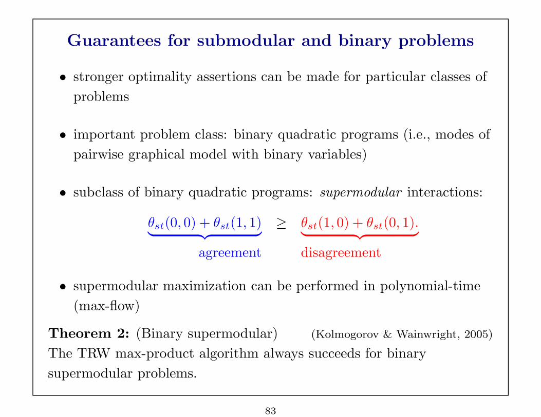
Guarantees for submodular and binary problems
• stronger optimality assertions can be made for particular classes of
problems
• important problem class: binary quadratic programs (i.e., modes of
pairwise graphical model with binary variables)
• subclass of binary quadratic programs: supermodular interactions:
θst(0, 0) + θst(1, 1)︸ ︷︷ ︸ ≥ θst(1, 0) + θst(0, 1).︸ ︷︷ ︸agreement disagreement
• supermodular maximization can be performed in polynomial-time
(max-flow)
Theorem 2: (Binary supermodular) (Kolmogorov & Wainwright, 2005)
The TRW max-product algorithm always succeeds for binary
supermodular problems.
83
Page 84
Partial information
Question: Can TRW message-passing still yield useful (partial)
information when strong tree agreement does not hold?
Theorem 2: (Binary persistence) (Kolmogorov & Wainwright, 2005; Hammer
et al., 1984)
Let S ⊆ V be the subset of vertices for which there exists a single point
x∗s ∈ arg maxxs
ν∗s (xs). Then for any optimal solution y ∈ OPT(θ∗), it
holds that ys = x∗s.
Some outstanding questions:
• what fraction of variables are correctly determined in “typical”
problems?
• do similar partial validity results hold for more general (non-binary)
problems?
84
Page 85
Some experimental results: amount of frustration
0
25
50
75
100
0 0.2 0.4 0.6 0.8 1
σ • d = 2
σ • d = 4
σ • d = 6
σ • d = 8
0
25
50
75
100
0 0.2 0.4 0.6 0.8 1
σ • d = 1
σ • d = 2
σ • d = 3
σ • d = 4
85
Page 86
Some experimental results: coupling strength
0
25
50
75
100
2 4 6 8 10
N = 4
N = 128
N = 8
0
25
50
75
100
0 2 4 6 8
N = 4
N = 128 N = 8
86
Page 87
Disparity computation in stereo vision
• estimate depth in scenes based on two (or more) images taken from
different positions
• one powerful source of stereo information:
– biological vision: disparity from offset eyes
– computer vision: disparity from offset cameras
• challenging (computational) problem: estimate the disparity at
each point of an image based on a stereo pair
• broad range of research in both visual neuroscience and computer
vision
87
Page 88
Global approaches to disparity computation
• wide range of approaches to disparity in computer vision (see, e.g.,
Scharstein & Szeliski, 2002)
• global approaches: disparity map based on optimization in an MRF
PSfrag replacements
θst(ds, dt)
θs(ds)θt(dt)
• grid-structured graph G = (V, E)
• ds ≡ disparity at grid position s
• θs(ds) ≡ image data fidelity term
• θst(ds, dt) ≡ disparity coupling
• optimal disparity map bd found by solving MAP estimation problem for
this Markov random field
• computationally intractable (NP-hard) in general, but TRW
max-product and other message-passing algorithms can be applied
88
Page 89
Middlebury stereo benchmark set
• standard set of benchmarked examples for stereo algorithms
(Scharstein & Szeliski, 2002)
• Tsukuba data set: Image sizes 384× 288× 16 (W ×H ×D)
(a) Original image (b) Ground truth disparity
89
Page 90
Comparison of different methods
(a) Scanline dynamic programming (b) Graph cuts
(c) Ordinary belief propagation (d) Tree-reweighted max-product
(a), (b): Scharstein & Szeliski, 2002; (c): Sun et al., 2002 (d): Weiss, et al., 2005;
90
Page 91
Summary and future directions
• variational methods are based on converting statistical and
computational problems to optimization:
(a) complementary to sampling-based methods (e.g., MCMC)
(b) a variety of new “relaxations” remain to be explored
• many open questions:
(a) prior error bounds available only in special cases
(b) extension to non-parametric settings?
(c) hybrid techniques (variational and MCMC)
(d) variational methods in parameter estimation
(e) fast techniques for solving large-scale relaxations (e.g., SDPs,
other convex programs)
91


![1 Unifying Message Passing Algorithms Under the Framework of … · 2019-12-06 · arXiv:1703.10932v4 [cs.IT] 5 Dec 2019 1 Unifying Message Passing Algorithms Under the Framework](https://static.documents.pub/doc/80x56/5f0c9f257e708231d4365116/1-unifying-message-passing-algorithms-under-the-framework-of-2019-12-06-arxiv170310932v4.jpg)


![Message Passing Algorithms for Compressed SensingarXiv:0907.3574v1 [cs.IT] 21 Jul 2009 Message Passing Algorithms for Compressed Sensing David L. Donoho Department of Statististics](https://static.documents.pub/doc/80x56/5f449d12b1253e2f764e59d5/message-passing-algorithms-for-compressed-sensing-arxiv09073574v1-csit-21-jul.jpg)


