Graphics Processor Unit (GPU) Accelerated Shallow Transparent Layer Detection in Optical Coherence Tomographic (OCT) images for real-time

Corneal Surgical Guidance

Tejas Sudharshan Mathai1, 2, John Galeotti1, 2, Samantha Horvath2, George Stetten1, 2

1 Department of Biomedical Engineering, Carnegie Mellon University, Pittsburgh, USA 2 Robotics Institute, Carnegie Mellon University, Pittsburgh, USA

tmathai@andrew.cmu.edu

Abstract. An image analysis algorithm is described that utilizes a Graphics Processor Unit (GPU) to detect in real-time the most shallow subsurface tissue layer present in an OCT image obtained by a prototype SDOCT corneal imaging system. The system has a scanning depth range of 6mm and can acquire 15 volumes per second at the cost of lower resolution and signal-to-noise ratio (SNR) than diagnostic OCT scanners. To the best of our knowledge, we are the first to experiment with non-median percentile filtering for simultaneous noise reduction and feature enhancement in OCT images, and we believe we are the first to implement any form of non-median percentile filtering on a GPU. The algorithm was applied to five different test images. On an average, it took ~0.5 milliseconds to preprocess an image with a 20th-percentile filter, and ~1.7 milliseconds for our second-stage algorithm to detect the faintly imaged transparent surface.

Keywords: OCT, image-guidance, real-time, GPU, percentile filter, surface detection.

1 Introduction

Spectral Domain Optical Coherence Tomography (SDOCT) is a non-invasive, non-contact imaging modality that has found great use in ophthalmology for corneal and retinal disease diagnosis. SDOCT uses near-infrared wavelengths, typically in the 800nm-1600nm range, to image sub-surface structures - including transparent surfaces - in soft tissue, such as those in the anterior segment of the eye and the retina. These light waves penetrate not only the clear cornea and lens, but also the opaque limbus, where important physiological processes take place at the intersection of the cornea, iris, and sclera. The basic acquisition unit of a SDOCT scanner is a one-dimensional axial scan (A-scan) along the beam path, but by rapidly steering the OCT beam, multiple A-scans can be combined to produce 2-D and 3-D high resolution cross-sectional images of the tissue. [1, 2] Over the past few years, there has been significant progress towards the creation of SDOCT systems that provide higher image acquisition speeds. Since OCT was first demonstrated in 1991, the A-scan rates have gone up from 400 Hz to 20 MHz in experimental systems. [3] Most of the commercially available SDOCT systems operate using line scan rates within 30 – 85 KHz to produce high quality 2D B-scan images. The fastest spectrometer-based SDOCT systems that have been developed operate with a dual camera configuration and a 500 KHz A-scan rate. [4] These SDOCT setups have been used to obtain 2D images and 3D volumes; for high resolution 3D volumetric scans, the acquisition time is still on the order of seconds. [5, 6, 7] However, most of the SDOCT systems today were developed for diagnosis rather than clinical surgery, and only a few attempts have been made to integrate real-time OCT into eye surgery. OCT systems have been previously combined with surgical microscopes in order to obtain cross-sections of the sclera and cornea, but these systems were used in a “stop and check” scenario rather than for real-time guidance. [8, 9] It is a challenge to integrate a SDOCT system into interactive eye surgery while satisfying clinicians’ needs and preferences for high resolution, high signal-to-noise ratio (SNR), and real-time frame rates. In order to produce higher resolution images, more samples of the target need to be acquired, and higher contrast images with better SNR require a longer exposure for each individual A-scan (longer dwell time at each spot on the target). [2] SDOCT images are inevitably affected by noise. [11-14] A tradeoff always exists between fast image acquisition and high image quality, and if the image acquisition speed is increased, then SNR will suffer. [7, 10] OCT scanners laterally sample a target by steering the beam across one or two dimensions in order to produce a 2D image or a 3D volume. Processing the samples from the target to create an image is also a computationally intensive task, and the total time it takes to

process the samples into an image can be higher than the line scan acquisition rate. There have been approaches to quickly process interferometer data into image volumes, and to render the analyzed OCT volumes at speeds suitable for real-time visualization, but for the most part, volumetric rendering still happens only post-process. In particular, attempts have been made to utilize Graphics Processing Units (GPUs) and Field-Programmable Gate Arrays (FPGAs) in order to improve the data processing and rendering. [15-22] Parallel programming approaches have also been followed to improve very high speed acquisition of OCT data, hide the data processing latency, and render 3D OCT volumes at real-time frame rates. [4, 20]

The focus of this paper is on a computationally simple image analysis algorithm that makes use of a Compute Unified Device Architecture (CUDA) enabled NVIDIA Quadro-5000 Graphics Processor Unit (GPU), which allows fast processing of 2D images to occur in real-time. Our algorithm will be integrated into a custom-built prototype SDOCT corneal imaging system that can scan 128,000 lines per second (128 kHz A-scan rate) with acceptable image quality (12-bits/pixel frequency sampling). Our implementation is tolerant of the low SNR in the images inherent with the necessarily short exposure times of the SDOCT spectrometer’s line-scan camera. The algorithm (diagrammed in Fig. 1) automatically detects the shallowest surface of an imaged structure in 1.4-3.2 milliseconds, depending on the dimensions of the image (as discussed later), and hence has real–time applications. The algorithm will be incorporated into our existing augmented-reality SDOCT system for intra-operative surgical guidance. [23] In the future, the detected first tissue surface layer will be rendered in OpenGL, and then overlaid within the surgical microscope viewing environment, so as to appear in-situ within the actual corneal structure to provide real-time 3D visualization and surgical guidance for clinicians.

Fig 1. A block diagram portraying the different stages in the algorithm. The CPU stages are shown in white blocks, while the GPU stages are shown in shaded blocks.

2 Methods

2.1 Prototype System Configuration

The prototype OCT system consists of an 840nm super luminescent diode (SLD) light source with 50nm bandwidth that feeds light into a broadband, single-mode fiber-optic Michelson Interferometer that splits the light into sample-arm and reference-arm sections. The sample-arm section interrogates the target sample being imaged. For this paper, the target sample was a static phantom model consisting of a piece of folded scotch tape embedded inside clear candle wax gel. Fig 2(a) shows a zoomed image of the phantom (with the embedded scotch-tape) as reconstructed by our OCT system. The reference-arm section physically matches the path length of the light traveling through the sample-arm section from the SLD source to the beginning of the target range in the sample. The light output from the sample arm and reference arm are combined back together in the interferometer, and fed into a spectrometer that measures the amplitudes of the individual frequency components of the received signal. The detected signal is processed into an A-scan 1D image, which is a depth profile of the various reflections of light from the distinct structural layers present in the sample. The A-scan represents a reflectivity profile along the beam for a fixed lateral scanning position of the scanning mechanism, and at a single fixed location on the target sample.

Multiple A-scans are collected to form a 2D cross-sectional image of the target sample region being imaged. [24] The prototype SDOCT system has a scan depth range of 6mm, and acquires A-scans at 128 kHz when scanning 15 volumes per second resulting in lower contrast, lower quality SDOCT images than typical SDOCT systems. We do this to satisfy the physical space requirements for real-time surgical guidance. The SLD source has a total light output of ~6.76 mW, but the light output progressively decreases as it passes through the fibers and components in the SDOCT system. The power at the output of the sample-arm is 2.851 mW. The light returned by the sample is combined with the light output from the reference-arm in the interferometer, which filters out the light scattered in the sample, preserving only the small percentage of light that directly interrogated the subsurface targets for analysis by the spectrometer, where the input power is on the order of 50-100 nW.

2.2 Image Analysis

Noise Reduction. As a result of the rapid acquisition time of our SDOCT system, the output images are affected by substantial speckle noise. Since the manufacturer of our SDOCT system applied a custom non-linear noise reduction algorithm to the images acquired by the system, we chose not to attempt to explicitly model the residual noise. Instead, we chose to implement a post-processing algorithm that is insensitive to the remaining noise in the images. The integration time for all the frequency signals at the detector is very short, < 8 ns, and this contributes to the noise. SDOCT SNR also inherently drops off with depth, of particular relevance to our system with its extra deep 6mm A-scan length. Since the SNR depends in part on the light output power being detected at the spectrometer and the detector sensitivity, it follows that a generated image will have more noise and less contrast if the detected light output at the spectrometer is low. [24] Consequently, due to the noisy background, the physical edge boundaries are difficult to discriminate in the images generated by our SDOCT system.

 

Fig 2. (a) A zoomed view of an original noisy OCT image (b) Zoomed view of a bilateral filtered image (left), and the detected surface (right), (c) Zoomed view of a median filtered image (left), and the detected surface (right), (d) Zoomed view of a 20th-percentile and Gaussian filtered image (left), and subsequent detected surface (right), (e) Zoomed view of an extremely noisy OCT image (left), and the 20th-percentile and Gaussian filtered output (right), which resulted in significant noise reduction.

Sufficiently fast conventional noise-reduction methods such as Gaussian blurring, or non-iterative edge-preserving smoothing methods such as Bilateral filtering, were unable to satisfactorily suppress the noise in the OCT images without substantial loss of contrast on the actual structures being scanned. When the surface detection algorithm (described next) was applied after bilateral filtering our test image, the detected shallow surface was false as shown in Fig 2 (b). Median filtering is one of the slowest non-iterative noise-reduction algorithms [25], and it is often used to remove speckle noise, but it also struggled with the large amplitude of the image noise, as shown in Fig 2 (c). A key insight into our problem is that while the background contains many pixels that are very bright due to noise,

a   b   c   d   e  

with several background patches containing over 50% bright noise pixels, these pixels are generally randomly scattered and intermixed with dark pixels. Only actual surfaces contain a large majority of bright pixels. Sharpening our images using a Laplacian filter (after smoothing using a Gaussian) did not improve our detection, albeit the contrast of the image improved. Since Laplacian filters approximate the second-order derivatives of the image [26], application of a Laplacian filter to the original image increased the noise by enhancing the intensity values of the noisy pixels in the background patches. So, a filter was required that would increase the edge contrast for any input image while darkening pixels that are not mostly surrounded by bright edge pixels. Percentile filers, also known as rank filters, are certainly not new to image processing, but aside from the Median filter, other percentile filters are typically not used directly for noise reduction or image restoration, but rather for more specialized tasks, such as estimating the statistical properties of image noise, surface relief etc. [27, 28, 29]

We believe that we are the first to apply non-median percentile filtering to OCT noise reduction, as well as to implement percentile filtering (for any purpose) on a GPU. For our particular OCT images, selecting 20th-percentile (first quintile) seemed to best suppress the noise while simultaneously increasing the contrast of the first surface in all of our images. The intensity of most pixels is adjusted by the percentile filter toward the dark end of the gray-level range, except for those pixels surrounded almost exclusively (≥80% of their neighbors) by bright pixels. The 20th percentile was calculated by first determining the ordinal rank n described by:

𝑛   = !  !""

×  N + !! (1)

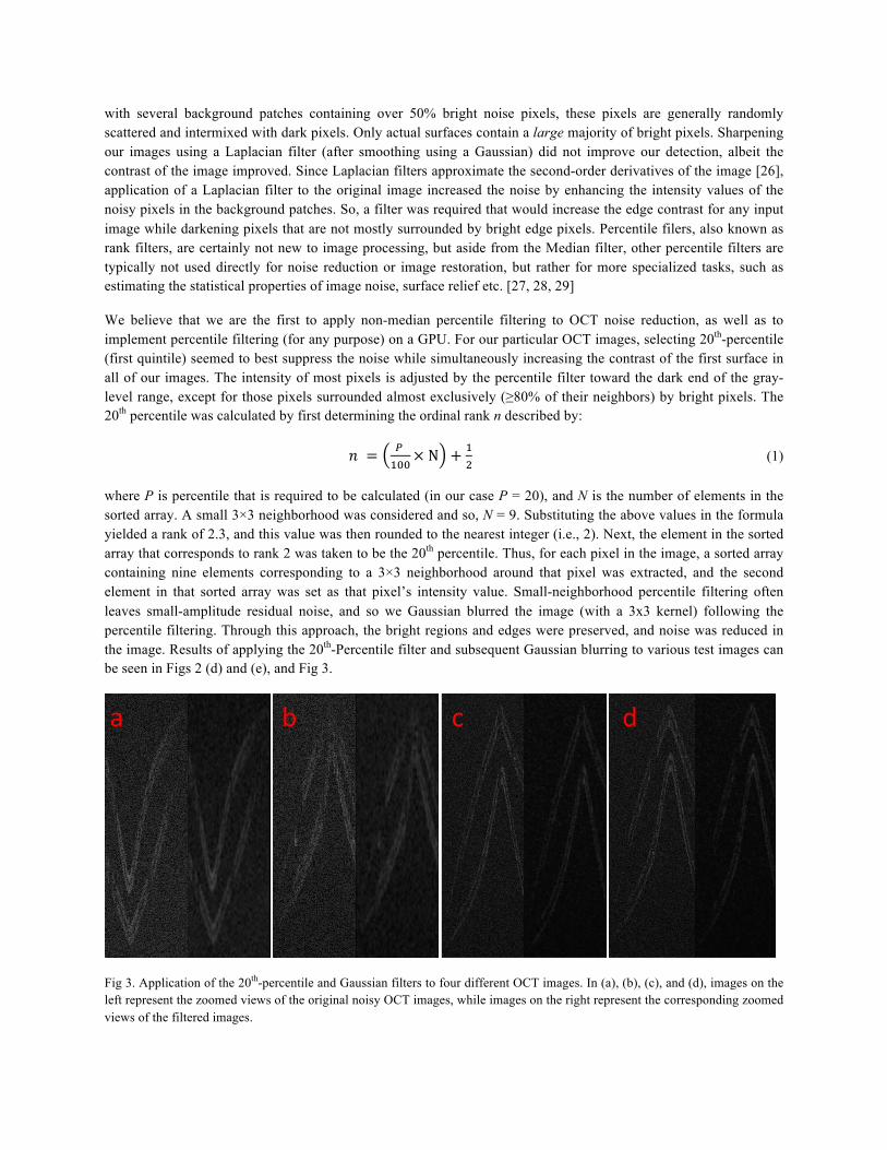
where P is percentile that is required to be calculated (in our case P = 20), and N is the number of elements in the sorted array. A small 3×3 neighborhood was considered and so, N = 9. Substituting the above values in the formula yielded a rank of 2.3, and this value was then rounded to the nearest integer (i.e., 2). Next, the element in the sorted array that corresponds to rank 2 was taken to be the 20th percentile. Thus, for each pixel in the image, a sorted array containing nine elements corresponding to a 3×3 neighborhood around that pixel was extracted, and the second element in that sorted array was set as that pixel’s intensity value. Small-neighborhood percentile filtering often leaves small-amplitude residual noise, and so we Gaussian blurred the image (with a 3x3 kernel) following the percentile filtering. Through this approach, the bright regions and edges were preserved, and noise was reduced in the image. Results of applying the 20th-Percentile filter and subsequent Gaussian blurring to various test images can be seen in Figs 2 (d) and (e), and Fig 3.

Fig 3. Application of the 20th-percentile and Gaussian filters to four different OCT images. In (a), (b), (c), and (d), images on the left represent the zoomed views of the original noisy OCT images, while images on the right represent the corresponding zoomed views of the filtered images.

a   b   c   d  

Fig 4. Results of the surface-detection algorithm. In (a), (b), (c), and (d), the original images are shown on the left while the detected surfaces are shown on the right.

Detection of Surfaces. The goal of our preprocessing is to enable very fast surface-detection for robust, real-time operation. After the input OCT image is 20th-percentile and Gaussian filtered, an Otsu threshold for the entire grayscale OCT image is computed using Otsu’s method. [30,31] Otsu’s original filter uses a bimodal histogram containing two peaks, which represent the foreground and the background, to model the original grayscale image. The filter then tries to find an optimal threshold that separates the two peaks so that the variance within each region is minimal. If there are L gray-levels in the OCT image [1, 2, 3…. L], then the within-class variance is calculated for each gray level. The within-class variance is defined as the sum of weighted variances of the two classes of pixels (foreground and background), and it is represented by:

𝜎!!(𝑡) =  𝑤! 𝑡 𝜎!!(𝑡) + 𝑤!(𝑡)𝜎!!(𝑡) (2)

where 𝜎!! is the within-class variance, 𝜎!! is the variance of a single (foreground or background) class, and 𝑤i is the weight that represents the probabilities of the two classes separated by the threshold t. The gray level value for which the sum of weighted variances is lowest is set as the Otsu threshold. This approach is computationally intensive as it involves an exhaustive search for the threshold among all the gray-levels present in the 8-bit grayscale OCT image. A faster approach to threshold selection, also described by Otsu, involves the computation of the between-class variance. Otsu showed that maximizing the between-class variance led to the same result as minimizing the within-class variance [29, 30], and the between-class variance is given by:

𝜎!! 𝑡  =  𝜎!! 𝑡 −  𝜎!! 𝑡 =  𝑤! 𝑡 𝑤! 𝑡 [𝜇! 𝑡 −  𝜇! 𝑡 ]2 (3)

where 𝜎!! is the between-class variance, 𝜎!! is the total variance of both classes, 𝑤! are the class probabilities, and 𝜇! are the class means respectively. 𝜎!! and 𝜎!! are functions of the threshold, while 𝜎!! is not.

The class probability 𝑤! 𝑡 is represented as a function of the threshold t by:

𝑤! 𝑡 =   𝑝!!! (4)

where 𝑝!  is the probability distribution, which was obtained by normalizing the gray-level histogram, and the class mean 𝜇! 𝑡 is calculated by:

𝜇! 𝑡 = 𝑝 𝑖!! 𝑥 𝑖 𝑤! (5)

a   b   c   d  

where  𝑥 𝑖 is the center of the ith histogram bin. Similarly, by using the same formulas above, 𝑤! 𝑡 and 𝜇! 𝑡 can be computed from the histogram for bins which are greater than t. The between-class variance calculation is a much faster and simpler approach to selecting a threshold that separates the foreground pixels from background pixels. Next, our surface detection algorithm performs a very efficient linear search along each individual column of the 20th-percentile filtered image for the first faintly visible surface. As the search iterates down each column (A-scan) in the preprocessed image, the algorithm compares each pixel’s intensity value with its neighbors, and based upon the computed Otsu threshold, it determines if the current pixel is present in the background or the foreground of the image. By efficiently utilizing the pre-determined Otsu threshold, the surface-detection algorithm correctly selects the first surface for the majority of the columns in the image. These individual selected pixel localizations (one per column) are then pruned of outliers (as described below), and connected together into one or more curved sections, each of which corresponds to an unambiguous physically continuous segment of the underlying surface.

Isolated single-pixel outliers were easily removed, but small clusters of connected outliers were more challenging to remove in real-time. Fortunately, these clusters tended to be physically separated from the actual surface of interest, and so, they could be implicitly excluded during the curve-connecting stage. Detected pixels were connected together so as to find only the surface of interest by first measuring the distance between each set of two detected points, and then connecting them together by a rendered line.  Sets of two points whose distance exceeded a given threshold were also connected together, but by a line of lower intensity, so that while the entire surface is automatically detected, there is also a visual cue to locations where ambiguity in the OCT image could possibly indicate that a small gap might be present in the physical tissue surface.

Table 1. Performance of the algorithm measured for five images.

Image Number

Dimension GPU execution time – 20th-Percentile Filter

(milliseconds)

GPU execution time –Surface Detection

(milliseconds)

CPU Execution Time –Surface Detection

(milliseconds) 1 256 x 1024 ~0.368 1.222 109 2 256 x 1024 ~0.368 1.218 93 3 256 x 1024 ~0.368 1.040 141 4 256 x 2048 ~0.727 2.475 172 5 256 x 2048 ~0.727 2.472 202

Average Execution Time (milliseconds)

~0.512 1.685 143.5

3 Results

The 20th-percentile filter, followed by Gaussian blurring, reduced large amounts of speckle noise in the image, which allowed the surface detection algorithm to quickly and accurately detect the shallowest surface present in the image. The surfaces detected by the algorithm for different images are shown in Fig 4, and the measured time it took to execute the entire algorithm on the GPU is shown in Table 1. The dimensions of B-scan OCT images that were passed as an input to the algorithm were varied, and this was intentionally done in order to measure the performance of the algorithm under this condition. On an average, the 20th-percentile filter implemented using CUDA on the GPU took ~0.512 milliseconds to execute. The detection of the surface from the 20th-percentile and Gaussian filtered image took ~1.7 milliseconds on average.

The surface-detection algorithm was also implemented on the CPU, and its performance was measured and found to be 143.5 milliseconds, on average. The original image and the detected curve’s mask were overlaid using ITK-SNAP [32] as seen in Fig 5. From the overlaid images, it is visually noticeable that most of the detected surfaces match with the curved structures in the original image, with the total computation time being less than 3.5 milliseconds. However, the algorithm is not perfect, and the noise present in the original low-contrast OCT images

does occasionally result in fractured surface detection as shown in Figs 5 and 6. The performance of the algorithm was timed using NVIDIA’s Visual Profiler v4.2 and NVIDIA’s Nsight Visual Studio Edition v3.2. On average, the total runtime of the program was 1.126 seconds, which included the low-bandwidth memory copies to and from the CPU and GPU. [33]

Fig 5. Zoomed results showing two different original images with overlaid surface detection. In (a) and (b), the detected curve (shown in red) for each test image was overlaid on the original image. By visual inspection, the detected curves line up well with the original edges.

Fig 6. Zoomed crops of the overlays for two different images in (a) and (b) show how a lack of differentiation in intensity between pixels representing an edge versus the background can cause the surface detection to be fractured by gaps.

4 Discussion and Future Directions

The dimensions of the image play a vital role in the performance of the percentile filter. For a 256x1024 pixel image, the execution times were measured for the PercentileFilterKernel and SurfaceDetectionKernel on the GPU; the filtering stage took ~369µs to filter the image, while the surface-detection stage took 1.22ms to execute. Unlike a CPU that is optimized to handle sequential code that is complex and branching, a GPU is optimized for the parallel application of one piece of code (a kernel) to many elements at once (e.g., to each pixel in an image). With a GPU, each pixel’s intensity value in the output image can be calculated by a dedicated thread, which is assigned to work on the corresponding pixel and its neighbors in the input image. As with a CPU, a GPU’s fastest memory is its on-chip registers and its slowest memory is the bulk global GPU memory. Also, just like a CPU can speed global memory access by using a cache (for example: L1 cache), a GPU can speed access to its global memory by allocating a dedicated high-speed shared memory to each block of threads. During runtime, a block of threads executed by a streaming multiprocessor (SM) on the GPU is further grouped into warps, where a warp is a group of

a   b  

a   b  

32 parallel threads. The use of shared memory allows global memory access to be coalesced by warps, and thereby improves the latency of the data fetches. As shared memory is present on-chip, it has a latency that is roughly 100x lower than uncached global memory access, and it is allocated per block, which allows all parallel threads in a block to have access to the same high-speed shared memory. [33] GPUs also permit traditional L1 caching of memory, but the GPU L1 cache still has inferior performance to per-block shared memory in terms of memory bandwidth. [34]

PercentileFilterKernel  –  Active  Thread  Occupancy    

 

SurfaceDetectionKernel  –  Active  Thread  Occupancy  

Fig 7. Graphs detailing the current active thread occupancy on the GPU for the PercentileFilterKernel and SurfaceDetectionKernel respectively. The red circle shows the algorithm’s active thread occupancy on the GPU as set against other theoretically calculated occupancy levels by NVIDIA’s Nsight Visual Studio Edition v3.2.

The active thread occupancy levels for our algorithm are displayed in Fig 7, and the red circle in each graph represents the runtime state of the GPU as dictated by our algorithm. Occupancy can be measured in terms of warps, and it is defined as the ratio of the current number of active warps running concurrently on a streaming multiprocessor (SM) to the maximum number of warps that can run concurrently. [33] For the PercentileFilterKernel, there are 48 warps active on our GPU with the maximum number of warps for our GPU being 48. Thus, the occupancy level for the Percentile Filter is 100%. From the graph detailing the varying block size for the PercentileFilterKernel, allocating 256 threads per block allowed an efficient coalesced global memory access. Out of these 256 threads per block, only 128 threads were used to load the neighbors of consecutive pixels to the shared memory. Each of these 128 threads processed a 3×3 or 5×5 neighborhood as set by the user, and loaded

them into shared memory. The remaining 128 threads in the same block would access the “shared” pixels that were previously loaded by the first set of 128 threads, thus effectively reducing the read operation by half, and at the same time, creating a very efficient memory access pattern. In the two Fig 7 graphs titled “Varied Shared Memory Usage”, the legend “L1” represents the cache memory present on the GPU, while the legend “Shared” represents the shared memory present on the GPU, as previously discussed. From the shared memory usage graph for the PercentileFilterKernel, it can be seen that the utilization of the shared memory on the GPU allows faster data access when compared to L1-cache memory of the GPU. Similarly, from the graphs for the SurfaceDetectionKernel, the occupancy was calculated to be 100%, with registers being sufficient so-as to not require or benefit from shared memory, and the active warp count equals the maximum number of warps running in parallel on the GPU. As seen from the varying block size graph for the SurfaceDetectionKernel, only 256 threads were used to detect the faintly visible surface. Each thread was allowed to process pixels only along a single column of the image. The thread extracted the values of the neighbors of a pixel, either in a 3×3 or 5×5 neighborhood as set by the user, loaded the values to memory, and used the computed Otsu threshold to determine if the pixel is present on the edge representing the phantom’s surface.

However, the percentile filtering stage of the algorithm can be further optimized. In future work, the sorting scheme employed by the 20th-percentile filter could be upgraded in order to boost the performance of the algorithm. Presently, a naïve bubble sorting implementation is used by the algorithm. A naïve bubble sort is efficient in cases where only a 3×3 or a 5×5 pixel neighborhood is being considered, and only half the elements stored in the sorting array are being sorted, leading to a runtime of O(n2/4). However, as the size of the sorting array increases with neighborhood size, it becomes more efficient to run other sorting algorithms, such as radix sort or quick sort. [35, 36] Moving beyond the detection of the first surface, detecting underlying surfaces poses a challenge because these surfaces do not always appear smoothly connected or visible in the image. There may be gaps in the image that actually represent a structure in the target tissue being imaged, and it is important to represent these gaps by appropriate marker(s) in the image. Future directions of this algorithm are directed towards detecting and analyzing these underlying surfaces robustly, even when physical discontinuities are occasionally present.

5 Conclusion

We have implemented a GPU-based algorithm capable of real-time detection of first surfaces in noisy SDOCT images, such as those acquired by our prototype SDOCT corneal imaging system that trades off an inherently lower SNR for high-speed acquisition of images spanning 6mm in depth. The algorithm requires ~0.5 milliseconds on average to percentile and Gaussian filter the image, and ~1.7 milliseconds on average to detect the first surface thereafter. The surface detection algorithm’s accuracy significantly depends on our preprocessing to reduce the speckle noise in the original image. More than 90% of the detected surface lies on the actual edge boundary. We are now incorporating our algorithm into a complete system for real-time corneal OCT image analysis and surgical guidance. Our implementation will enable clinicians to have an augmented-reality in-situ view of otherwise invisible tissue structures and surfaces during microsurgery.

Acknowledgements. This work was funded in part by NIH grants #R01EY021641 and #R21-EB007721, a grant from Research to Prevent Blindness, and a NSF graduate student fellowship.

References

1. LaRocca F., Izzat J.: Handheld simultaneous scanning laser ophthalmoscopy and optical coherence tomography system. Biomed. Opt. Express. 4, 2307-2321, (2013)

2. Fang L., Izzat J.: Fast Acquisition and Reconstruction of Optical Coherence Tomography Images via Sparse Representation. IEEE Trans. Act. Med. Imaging. 32, 2034 - 2049, (2013)

3. Drexler W., Fujimoto J. G.: State-of-the-art retinal optical coherence tomography. Progr. Retinal Eye Res. 27, 45–88 (2008)

4. Jian Y., Sarunic M.: Graphics processing unit accelerated optical coherence tomography processing at megahertz axial scan rate and high resolution video rate volumetric rendering. J. Biomed. Opt. 18, 026002-026002 (2013)

5. An L.: High speed spectral domain optical coherence tomography for retinal imaging at 500,000 A-lines per second. Biomed. Opt. Express. 2, 2770–2783 (2011)

6. Ricco S., Chen M., Schuman J.: Correcting motion artifacts in retinal spectral domain optical coherence tomography via image registration. In: MICCAI 2009. G.-Z. Yang, D. Hawkes, D. Rueckert, A. Noble, and C. Taylor (eds.). 12, Part 1, 100–107, Springer, Heidelberg (2009)

7. Robinson M. D., Izatt J., Farsiu S.: Novel applications of super-resolution in medical imaging. In: Super-resolution imaging, P. Milanfar (ed.), CRC Press, 383–412, (2010)

8. Tao Y., Izzat J.: Intraoperative spectral domain optical coherence tomography for vitreoretinal surgery. Opt. Lett. 35, 3315–3317, (2010)

9. Geerling G.: Intraoperative 2-Dimensional Optical Coherence Tomography as a New Tool for Anterior Segment Surgery. Arch. Ophthalmol., 123, 253-257 (2005)

10. McNabb R. P., Farsiu S., Izatt J.: Distributed scanning volumetric SDOCT for motion corrected corneal biometry. Biomed. Opt. Exp., 3, 2050–2065, (2012)

11. Gargesha M., Jenkins M. W., Rollins A. M., Wilson D. L.: Denoising and 4D visualization of OCT images. Opt. Exp. 16, 12313–12333, (2008)

12. Jian Z., Yu L., Rao B., Chen Z.: Three-dimensional speckle suppression in optical coherence tomography based on the curvelet transform. Opt. Exp. 18, 1024–1032, (2010)

13. Wong A., Mishra A., Bizheva K., Clausi D. A.: General Bayesian estimation for speckle noise reduction in optical coherence tomography retinal imagery. Opt. Exp. 18, 8338–8352, (2010)

14. Salinas H. M., Fernández D. C.: Comparison of PDE-based nonlinear diffusion approaches for image enhancement and denoising in optical coherence tomography. IEEE Trans. Med. Imag. 26, 761–771, (2007)

15. Lee K. K. C.: Real-time speckle variance swept-source optical coherence tomography using a graphics processing unit. Biomed. Opt. Express. 3, 1557–1564 (2012)

16. Li J., Bloch P.: Performance and scalability of Fourier domain optical coherence tomography acceleration using graphics processing units. Appl. Opt. 50, 1832–1838 (2011)

17. Rasakanthan J., Sugden K., Tomlins P. H.: Processing and rendering of Fourier domain optical coherence tomography images at a line rate over 524 kHz using a graphics processing unit. J. Biomed. Opt. 16, 020505 (2011)

18. Sylwestrzak M.: Real-time massively parallel processing of spectral optical coherence tomography data on graphics processing units. In: Proceedings of SPIE - Optical Coherence Tomography and Coherence Techniques, 8091, (2011)

19. Watanabe Y., Itagaki T.: Real-time display on Fourier domain optical coherence tomography system using a graphics processing unit. J. Biomed. Opt. 14, 060506 (2009)

20. Zhang K., Kang J. U.: Graphics processing unit-based ultrahigh speed real-time Fourier domain optical coherence tomography. IEEE J. Sel. Topics Quantum Electron. 18, 1270–1279 (2012)

21. Desjardins A. E.: Real-time FPGA processing for high-speed optical frequency domain imaging. IEEE Trans. Med. Imag. 28, 1468–1472 (2009)

22. Ustun T. E.: Real-time processing for Fourier domain optical coherence tomography using a field programmable gate array. Rev. Sci. Instrum. 79, 114301 (2008)

23. Galeotti J., Schuman J., Siegel M., Wu B., Klatzky R., Stetten G.: The OCT-Penlight: In-Situ Image Display for Guiding Microsurgery using Optical Coherence Tomography (OCT), SPIE Medical Imaging, 7625-1 (2010)

24. Izatt J. A., Choma M. A.: Theory of Optical Coherence Tomography, Optical Coherence Tomography: Technology and Applications. Part 1, 47-72, (2008)

25. Huang, T., Yang, G., Tang, G.: A fast two-dimensional median filtering algorithm. IEEE Trans. Acoust. Speech. Signal Process. 27, 13-18 (1979)

26. Shapiro L., Stockman G.: Computer Vision. Prentice Hall (2001) 27. Colom M., Buades A.: Analysis and Extension of the Percentile Method, Estimating a Noise Curve from a Single

Image. Image Proc. On Line. 3, 332–359 (2013) 28. Percentile Filter, http://www.uoguelph.ca/~hydrogeo/Whitebox/Help/FilterPercentile.html 29. Percentile, Wikipedia, http://en.wikipedia.org/wiki/Percentile 30. Otsu N.: A threshold selection method from gray-level histograms. IEEE Trans. Sys., Man., Cyber. 9, 62–66 (1979) 31. Otsu’s Method, Wikipedia, http://en.wikipedia.org/wiki/Otsu's_method 32. Yushkevich P., Piven J., Gee J., Gerig G.: User-guided 3D active contour segmentation of anatomical structures:

Significantly improved efficiency and reliability. Neuroimage. 31, 1116-1128 (2006). 33. NVIDIA, CUDA C Best Practices Guide. 34. NVIDIA, CUDA C Programming Guide. 35. Sedgewick R.: Algorithms in C++. Addison-Wesley (1998) 36. Sedgewick R.: Implementing Quicksort Programs. Comm. ACM. 21, 847-857 (1978).