© M

arku

s Net

eler

 200

6 ­ C

C­BY

­SA

The GRASS GIS software

GIS Seminar

Politecnico di Milano

Polo Regionale di Como

M. Netelerneteler at itc ithttp://mpa.itc.ithttp://grass.itc.it

ITC-irst, Povo (Trento), Italy

(Document revised November 2006)

© M

arku

s Net

eler

 200

6 ­ C

C­BY

­SA

GRASS: Geographic Resources Analysis Support System

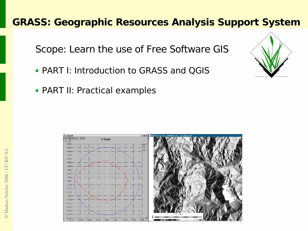
Scope: Learn the use of Free Software GIS

PART I: Introduction to GRASS and QGIS

PART II: Practical examples

© M

arku

s Net

eler

 200

6 ­ C

C­BY

­SA

GRASS: Geographic Resources Analysis Support System

Free Software GIS (“software libero”):

GRASS master Web site is in Italy: http://grass.itc.it

Portable: Versions for GNU/Linux, MS-Windows, Mac OSX, SUN, etc

Programming: Programmer's Manual on Web site (PDF, HTML), generated weekly. Code is documented in source code files (doxygen)

Sample data

Mailing lists in various languages

Commercial support

© M

arku

s Net

eler

 200

6 ­ C

C­BY

­SA

GRASS GIS

Brief Introduction

Developed since 1984, always Open Source, since 1999 under GNU GPL

Written in C programming language, portable code (multi-OS, 32/64bit)

International development team, since 2001 coordinated at ITC-irst

GRASS master Web site:

http://grass.itc.it

GNU/Linux

MacOSXMS-Windows

iPAQ

© M

arku

s Net

eler

 200

6 ­ C

C­BY

­SA

What's GRASS GIS?

● Raster and 2D/3D topological vector GIS

● Voxel support (raster 3D volumes)

● Vector network analysis support

● Image processing system

● Visualization system

● DBMS integrated (SQL) with dbf, PostgreSQL, MySQL and sqlite drivers

● In GRASS 6.1 translationsof the user interface to 16 languages ongoing

● Interoperability: supports all relevant raster and vector formats

From DXF

© M

arku

s Net

eler

 200

6 ­ C

C­BY

­SA

Spatial Data Types

Supported Spatial Data Types

2D Raster data incl. image processing 3D Voxel data for volumetric data

2D/3D Vector data with topology Multidimensional points data

http://grass.itc.it

Orthophoto

Distances

Vector TIN

3D Vector buildings

Voxel

© M

arku

s Net

eler

 200

6 ­ C

C­BY

­SA

Raster data model

Raster geometry

cell matrix with coordinates resolution: cell width / height (can be in kilometers, meters, degree etc.)

y resolution

x resolution

© M

arku

s Net

eler

 200

6 ­ C

C­BY

­SA

Vector data model

Vector geometry types

Point Centroid Line Boundary Area (boundary + centroid) face (3D area) [kernel (3D centroid)] [volumes (faces + kernel)]

Geometry is true 3D: x, y, z

Node

Node

Vertex

Vertex

Segment

Segm

ent

Segment

Node

Boundary

Vertex

Vertex

Vertex

Vertex

Centroid

Area

Line

Faces

not i

n al

l GIS

!

© M

arku

s Net

eler

 200

6 ­ C

C­BY

­SA

OGC Simple Features versus Vector Topology

Simple Features ...

- points, lines, polygons- replicated boundaries for adjacent areas

Advantage:- faster computations

Disadvantage:- extra work for data maintenance- in this example the duplicated boundaries are causing troubles Switzerland

slivers

Map generalized withDouglas-Peucker algorithmin non-topological GIS

gaps

(Latitude-longitude)

© M

arku

s Net

eler

 200

6 ­ C

C­BY

­SA

OGC Simple Features versus Vector Topology

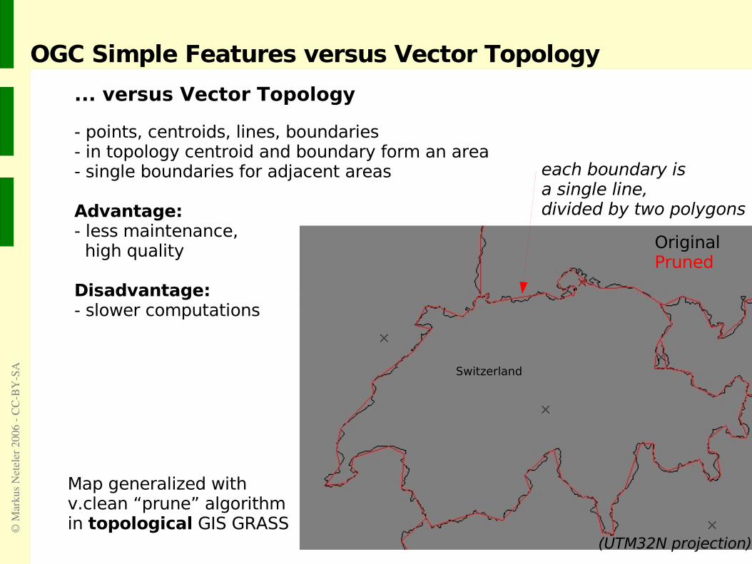
... versus Vector Topology

- points, centroids, lines, boundaries- in topology centroid and boundary form an area- single boundaries for adjacent areas

Advantage:- less maintenance, high quality

Disadvantage:- slower computations

Switzerland

OriginalPruned

each boundary is a single line,divided by two polygons

(UTM32N projection)

Map generalized withv.clean “prune” algorithmin topological GIS GRASS

© M

arku

s Net

eler

 200

6 ­ C

C­BY

­SA

Italy: Gauss-Boaga Coordinate System

Gauss-Boaga

Transverse Mercator projection 2 zones (fuso Ovest, Est) with a width of 6º30' longitude Each zone is an own projection!

False easting: Fuso Ovest: 1500000m (1500km) Fuso Est: 2520000m (2520km)

False northing: 0m

Scale along meridian: 0.9996 – secante case, not tangent case Ellipsoid: international (Hayford 1909, also called International 1924)

Geodetic datum: Rome 1940 (3 national datums; local datums to buyfrom IGM). National datum values available at:http://crs.bkg.bund.de/crs-eu/

© M

arku

s Net

eler

 200

6 ­ C

C­BY

­SA

Italy: Gauss-Boaga Fuso Ovest

ESRI PRJ-File for Fuso Ovest (g.proj -w in GRASS)

PROJCS["Monte_Mario_Italy_1", GEOGCS["GCS_Monte_Mario", DATUM["Monte_Mario", SPHEROID["International_1924",6378388,297]], PRIMEM["Greenwich",0], UNIT["Degree",0.017453292519943295]], PROJECTION["Transverse_Mercator"], PARAMETER["False_Easting",1500000], PARAMETER["False_Northing",0], PARAMETER["Central_Meridian",9], PARAMETER["Scale_Factor",0.9996], PARAMETER["Latitude_Of_Origin",0], UNIT["Meter",1]]

EPSG codes: Gauss-Boaga/Monte Mario 1: EPSG 26591 Gauss-Boaga/Monte Mario 2: EPSG 26592

© M

arku

s Net

eler

 200

6 ­ C

C­BY

­SA

Geodetic Datums of Gauss-Boaga

Geodetic datum: “peninsular datum”

"Monte Mario to WGS 84 (4)","Position Vector 7-param. transformation","X-axis translation","1","-104.1","metre","Italy - mainland""Y-axis translation","2","-49.1","metre","Italy - mainland""Z-axis translation","3","-9.9","metre","Italy - mainland""X-axis rotation","4","0.971","arc-second","Italy - mainland""Y-axis rotation","5","-2.917","arc-second","Italy - mainland""Z-axis rotation","6","0.714","arc-second","Italy - mainland""Scale difference","7","-11.68","parts per million","Italy - mainland"

also available: Sardegna, Sicilia

© M

arku

s Net

eler

 200

6 ­ C

C­BY

­SA

How to use GRASS GIS?

GRASS startup screen

© M

arku

s Net

eler

 200

6 ­ C

C­BY

­SA

GRASS: Modernized GIS manager and WMS support

gis.m: Michael Barton, Cedric Shockr.in.wms: Sören Gebbert & Jachym Cepicky

© M

arku

s Net

eler

 200

6 ­ C

C­BY

­SA

GRASS integration with QGIS

http://qgis.orgQGIS-GRASS plugin: Radim Blazek

© M

arku

s Net

eler

 200

6 ­ C

C­BY

­SA

WebGIS: Integration of data sources

GRASS in the Web

Real-time monitoring of Earthquakes (provided in Web by USGS)with GRASS/PHP: http://grass.itc.it/spearfish/php_grass_earthquakes.php

© M

arku

s Net

eler

 200

6 ­ C

C­BY

­SA

Raster Vector CAD WebGISGeoTIFF DGN DXF Web Map Service (WMS)Erdas IMG ESRI-SHAPE DWG Web Coverage Service (WCS)MrSID GML ... Web Feature Service (WFS)ECW Spatial SQL Web Map Context Documents (WMC)JPEG2000 ......

GRASS GIS Interoperability

Data models and formats

GDAL OGR openDWG Mapserver

GRASS PROJ.4

© M

arku

s Net

eler

 200

6 ­ C

C­BY

­SA

WebGIS: Integration of data sources

GIS – DBMI – Mapserver linking

WMS/WFS/WMC/SLD

Internet users

Raster:GeoTIFF,IMG, ...

Vector:SHAPE,MapInfo,...

Web Services

PostGIS ArcSDE

Oracle Sp.

GRASS

Raster

Vector/DBMI

© M

arku

s Net

eler

 200

6 ­ C

C­BY

­SA

Part II

Practical examples

● GRASS startup● User interface● NVIZ visualization● Raster data processing● Vector map applications● Image processing

DATA download: http://mpa.itc.it/markus/osg05/

© M

arku

s Net

eler

 200

6 ­ C

C­BY

­SA

Command structure

GRASS Command Overview

prefix functionclass

type of command example

d.* display graphical output d.rast: views raster mapd.vect: views vector map

db.* database databasemanagement

db.select: selects value(s) from table

g.* general general fileoperations

g.rename: renames map

i.* imagery image processing i.smap: image classifier

ps.* postscript map creation inPostscript format

ps.map: map creation

r.* raster raster dataprocessing

r.buffer: buffer around rasterfeaturesr.mapcalc: map algebra

r3.* voxel raster voxel dataprocessing

r3.mapcalc: volume map algebra

v.* vector vector dataprocessing

v.overlay: vector map intersections

© M

arku

s Net

eler

 200

6 ­ C

C­BY

­SA

Some things you should know about GRASS

● Import of data: GRASS always import the complete map

● Export of data: ● Vector maps: always the entire map is exported (cut before if needed)● Raster maps: r.out.gdal always exports entire map at original resolution

r.out.tiff (etc.) export at current region and resolution

What's a region in GRASS?● The default region is the standard settings of a GRASS location which is

essentially independent from any map● A region is the current working area (user selected resolution and coordinate

boundaries)● All vector calculations are done at full vector map● All raster calculations are done at current resolution/region. To do calculations

at original raster map resolution/region, the easiest way is touse 'g.region' first to set current region to map(see next slides)

GRASS Location “italy”

GRASS Mapset “northeast”

GRASS Mapset “sardegna”

© M

arku

s Net

eler

 200

6 ­ C

C­BY

­SA

Spearfish Sample Dataset

SD

SpearfishSpearfish (SD) sample data location

Maps:● raster, vector and point data ● covering two 1:24000 topographic

maps (quadrangles Spearfish and Deadwood North) ● UTM zone 13N, transverse mercator projection, Clarke66 ellipsoid, ● NAD27 datum, metric units, boundary coordinates:

4928000N, 4914000S, 590000W, 609000E DATA download: http://mpa.itc.it/markus/osg05/

© M

arku

s Net

eler

 200

6 ­ C

C­BY

­SA

Practical GIS Usage

Start a “terminal” to enter commands

Start GRASS 6 within the terminal:

grass61 -help

grass61 -gui

/ramdisk/grass/locations/

1.

2.

3.

© M

arku

s Net

eler

 200

6 ­ C

C­BY

­SA

GRASS user interface: QGIS

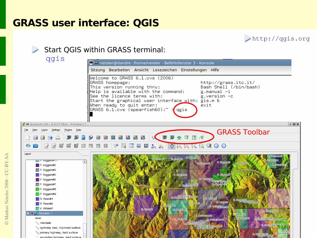
Start QGIS within GRASS terminal:qgis

http://qgis.org

GRASS Toolbar

© M

arku

s Net

eler

 200

6 ­ C

C­BY

­SA

QGIS: further key functionality

Creating a paper map

GRASS toolbox GRASS raster maps

GRASS vector maps GRASS vector digitizer

© M

arku

s Net

eler

 200

6 ­ C

C­BY

­SA

New GRASS user interface: QGIS

Excercise:

Please reproduce this map view!

Raster:- elevation.dem- aspect

Vector:- roads- fields

© M

arku

s Net

eler

 200

6 ­ C

C­BY

­SA

QGIS map composer: prepare map with layout

Creating a paper map for printing or saving into a file (SVG, PNG, Postscript)

Transfer map view into map composer (printer symbol)

© M

arku

s Net

eler

 200

6 ­ C

C­BY

­SA

QGIS: further key functionalityVector map visualization Raster map viz. PostGIS map viz.

WMS viz. Map query Vector object selection Attribute table

© M

arku

s Net

eler

 200

6 ­ C

C­BY

­SA

QGIS: GRASS toolboxGRASS toolbox

© M

arku

s Net

eler

 200

6 ­ C

C­BY

­SA

QGIS-GRASS Exercises: Noise impact 1/4

1) Simple noise impact map:

Extract interstate (highway) from roads vector map into new map and buffer interstate for 3km in each direction

GRASS commands:

a) first look at the table to get column name and ID of interstate:v.db.select roads

b) we extract only 'interstate' (cat = 1, cat is the GRASS standard column name for ID):v.extract in=roads out=interstate where=”cat = 1”

c) we buffer the interstate (give buffer in map units which is meters here):v.buffer interstate out=interstate_buf3000 buffer=3000

© M

arku

s Net

eler

 200

6 ­ C

C­BY

­SA

QGIS-GRASS Exercises: Noise impact 2/4

2) Verify affected areas:

Look at landcover.30m raster map,overlay extracted interstateand overlay buffered interstate_buf3000 (use transparency to make it nice)

© M

arku

s Net

eler

 200

6 ­ C

C­BY

­SA

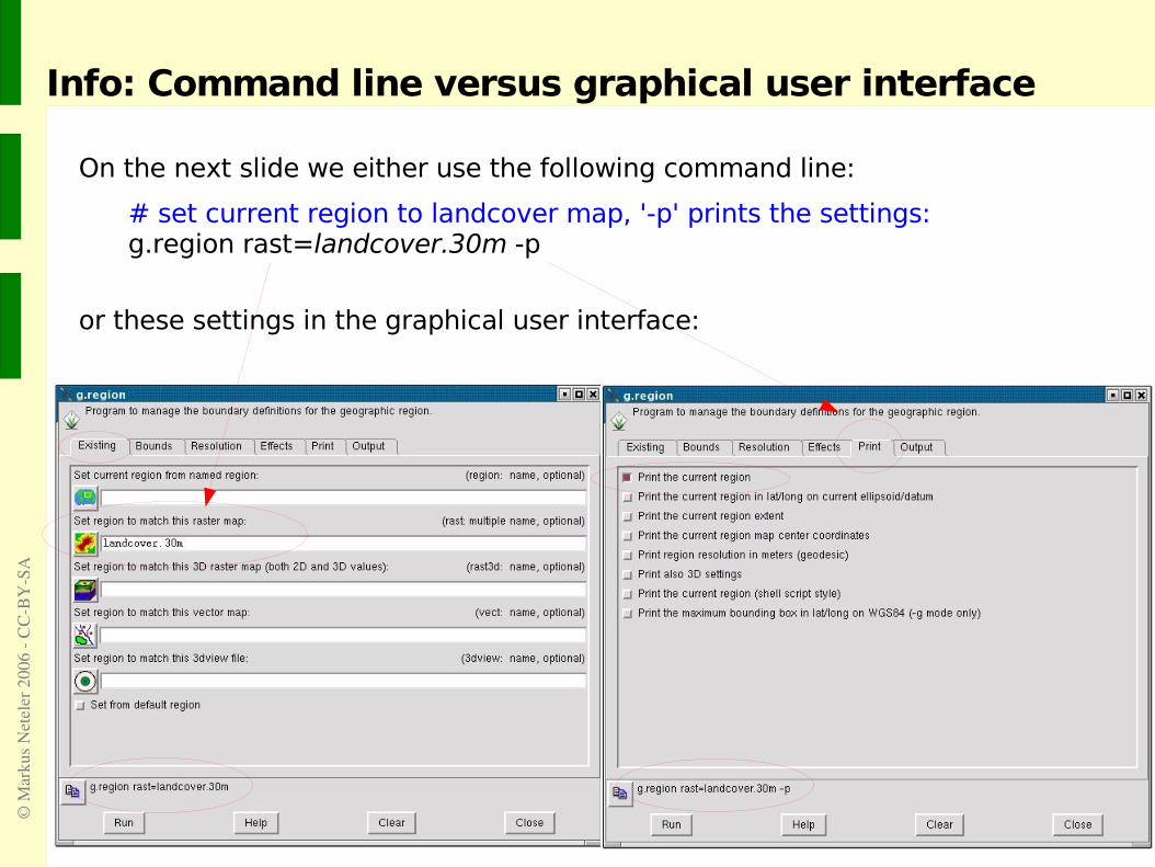
# set current region to landcover map, '-p' prints the settings:g.region rast=landcover.30m -p

Info: Command line versus graphical user interface

On the next slide we either use the following command line:

or these settings in the graphical user interface:

© M

arku

s Net

eler

 200

6 ­ C

C­BY

­SA

QGIS-GRASS Exercises: Noise impact 3/4How to get statistics on influenced landcover-landuse units?-> needs generalization of original landcover.30m map (originates from

satellite map)

Approach 1: Raster based generalization: “mode” operator in moving window

# set current region to landcover map, '-p' prints the settings:g.region rast=landcover.30m -pr.neighbors in=landcover.30m out=landcover.smooth method=mode size=3

3x3 moving window

© M

arku

s Net

eler

 200

6 ­ C

C­BY

­SA

QGIS-GRASS Exercises: Noise impact 4/4... Generalization cont'ed:

Approach 2: Vector based generalization: “rmarea” tool: merges small areas into bigger a.

# zoom to map:g.region rast=landcover.30m -p# raster to vector conversion:r.to.vect in=landcover.30m out=landcover_30m f=area# filter perimeter of 3x3 pixels ( threshold=(30 * 3)^2 = 8100)v.clean in=landcover_30m out=landcover_30m_gen tool=rmarea thresh=8100

© M

arku

s Net

eler

 200

6 ­ C

C­BY

­SA

Perspective view of maps

nviz el=elevation.dem vect=roads

© M

arku

s Net

eler

 200

6 ­ C

C­BY

­SA

GRASS: Geographic Resources Analysis Support System

Database: contains all GRASS data

Each GRASS project is organized in a „Location“ directory with subsequent„Mapset(s)“ subdirectories:

• Location: contains all spatial/attribute data of a geographically defined region (= project area)

• Mapset(s): used to subdivide data organization e.g. by user names, subregions or access rights (workgroups)

• PERMANENT: The PERMANENT mapset is a standard mapset which contains the definitions of a location. May also contain general cartography as it is visible to all users

Multi-User support: multiple users can work in a single location usingdifferent mapsets. Access rights can be managed per user. No user canmodify/delete data of other users.

Location and Mapset: “GRASS speech”

© M

arku

s Net

eler

 200

6 ­ C

C­BY

­SA

GRASS: Geographic Resources Analysis Support System

Example for Location and Mapsets

/home/user/grassdata

/europa

/hannover

/world

histdblncoor

sidx

topo

MapsetLocation

/PERMANENT

GRASS Database

/prov_trentino /PERMANENT

/trento

Geometry and attribute data

streets

parks

lakes

poi

streets.dbf

parks.dbf

poi.dbf

lakes.dbf

fcell

hist

colr

cell_misc

cellhd

cell

cats

vector

dbf

/silvia

© M

arku

s Net

eler

 200

6 ­ C

C­BY

­SA

Raster map analysis

➢ DEM analysis

➢ Raster map algebra

➢ Geocoding of scanned map

➢ Volume data processing

© M

arku

s Net

eler

 200

6 ­ C

C­BY

­SA

GRASS Command Classes

d.* display graphical output (screen)

r.* raster raster data processingr3.* raster3D raster voxel 3D data processingi.* imagery image processingv.* vector vector data processing

g.* general general file operations (copy, rename of maps, ...)m.* misc miscellaneous commands

ps.* postscript map creation in Postscript format

Prefix Class Functionality

© M

arku

s Net

eler

 200

6 ­ C

C­BY

­SA

Raster data analysis: Slope and aspect from DEM

Calculating slope and aspect from a DEM

# First we reset the current GRASS region settings to the input map: g.region rast=elevation.10m -p

r.slope.aspect el=elevation.10m as=aspect.10m sl=slope.10m

d.rast aspect.10md.rast.leg slope.10m

Note: horizontal angles are counted counterclockwise from the East

Slopes are calculated by default in degrees

Also curvatures can be calculated

0° East360°

+

© M

arku

s Net

eler

 200

6 ­ C

C­BY

­SA

Raster data analysis: Geomorphology

DEM: r.param.scale

# set region/resolution to the input map:g.region rast=elevation.10m -p

# generalize with size parameterr.param.scale elevation.10m out=morph \ param=feature size=25

# with legendd.rast.leg morph

# view with aspect/shade map (or QGIS)d.his h=morph i=aspect.10m

Spearfish DEM: 10mMoving window size: 25x25

nviz elev=elevation.10m col=morph

© M

arku

s Net

eler

 200

6 ­ C

C­BY

­SA

Raster data analysis: Water flows - Contributing area

Topographic Index: ln(a/tan(beta))

g.region rast=elevation.10m -p r.topidx in=elevation.10m out=ln_a_tanB

d.rast ln_a_tanB d.vect streams col=yellow # ... the old vector stream map nicely deviates from the newer USGS DEM

nviz elevation.10m col=ln_a_tanB

© M

arku

s Net

eler

 200

6 ­ C

C­BY

­SA

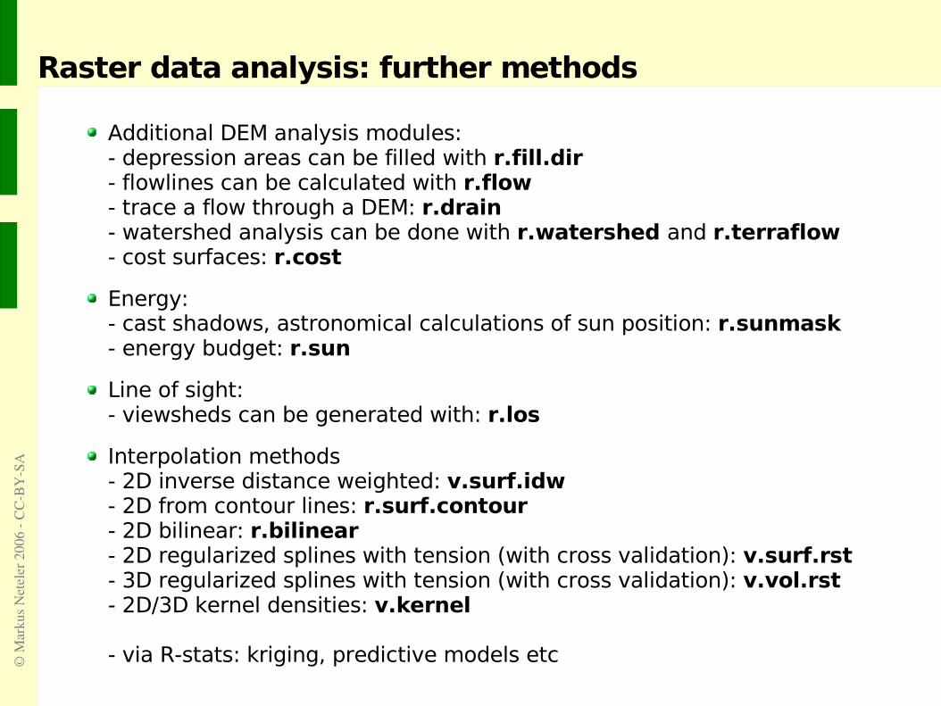
Raster data analysis: further methods

Additional DEM analysis modules:- depression areas can be filled with r.fill.dir- flowlines can be calculated with r.flow- trace a flow through a DEM: r.drain- watershed analysis can be done with r.watershed and r.terraflow- cost surfaces: r.cost

Energy:- cast shadows, astronomical calculations of sun position: r.sunmask- energy budget: r.sun

Line of sight:- viewsheds can be generated with: r.los

Interpolation methods- 2D inverse distance weighted: v.surf.idw- 2D from contour lines: r.surf.contour- 2D bilinear: r.bilinear- 2D regularized splines with tension (with cross validation): v.surf.rst- 3D regularized splines with tension (with cross validation): v.vol.rst- 2D/3D kernel densities: v.kernel

- via R-stats: kriging, predictive models etc

© M

arku

s Net

eler

 200

6 ­ C

C­BY

­SA

Raster map algebra

A powerful raster map algebra calculator is r.mapcalcSee for functionality:

g.manual r.mapcalc &

With a simple formula we filter all pixels with elevation higher than 1500m from the Spearfish DEM:

r.mapcalc "elev_1500 = if(elevation.dem > 1500.0, elevation.dem, null())”d.rast elev_1500

d.rast aspectd.rast -o elev_1500

© M

arku

s Net

eler

 200

6 ­ C

C­BY

­SA

Volume map processing: Demo

GRASS was enhanced to process and visualize Volumes(consisting of 3D voxels)

Functionality:

3D import/export

3D Regularized Splines with Tension interpolation

3D map algebra

NVIZ volume visualization: Isosurfaces and Profiles

© M

arku

s Net

eler

 200

6 ­ C

C­BY

­SA

Working with vector data

➢ Vector map import

➢ Attribute management

➢ Buffering

➢ Extractions, selections, clipping, unions, intersections

➢ Conversion raster-vector and vice verse

➢ Digitizing in GRASS and QGIS

➢ Working with vector geometry

© M

arku

s Net

eler

 200

6 ­ C

C­BY

­SA

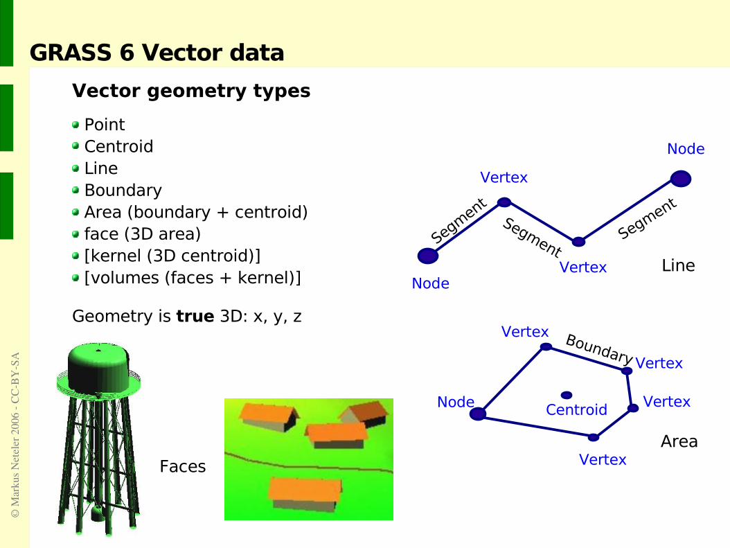
GRASS 6 Vector data

Vector geometry types

Point Centroid Line Boundary Area (boundary + centroid) face (3D area) [kernel (3D centroid)] [volumes (faces + kernel)]

Geometry is true 3D: x, y, z

Node

Node

Vertex

Vertex

Segment

Segm

ent

Segment

Node

Boundary

Vertex

Vertex

Vertex

Vertex

Centroid

Area

Line

Faces

© M

arku

s Net

eler

 200

6 ­ C

C­BY

­SA

Raster-Vector conversion – extraction 1/2

Extraction of residential areas from raster landuse map

# set current region to map; look at the landuse/landcover map with legend: g.region rast=landcover.30m -p d.erase d.rast.leg -n landcover.30m

# Automated vectorization of the landuse/landcover map: r.to.vect -s landcover.30m out=landcover30m feature=area

# see attribute table ('-p' prints the current connection between vector # geometry and attribute table – note that GRASS can link to various DBMS): v.db.connect -p landcover30m # ... will tell you that it is a DBF table v.db.select landcover30m

© M

arku

s Net

eler

 200

6 ­ C

C­BY

­SA

Raster-Vector conversion – extraction 2/2

Extraction of residential areas from raster landuse map

# generate list of unique landuse/landcover types from text legend output: v.db.select landcover30m | sort -t '|' -k2 -n -u

#display selected categories: d.erase d.vect landcover30m \

where="value=21 or value=22" \fcol=orange

# Extract residential area into a new vector map: v.extract landcover30m out=residential where="value=21 or value=22"

d.frame -e d.vect residential fcol=orange \ type=area d.vect roads d.barscale -mt

This pipe '|' character is a nice way ofcombining Unix commands. The output

of the first command is sent into the second and so forth...

sort is here sorting by second column on numbers (-n) and extracts

unique (-u) rows only

© M

arku

s Net

eler

 200

6 ­ C

C­BY

­SA

Creating/modifying vector maps

Digitizing in GRASS

Alternative:QGIS digitizer!

2 1

g.region rast=landcover.30m -pv.digit -n map=cities \ bg="d.rast landcover.30m"

1. define table set snapping threshold2. start digitizing

© M

arku

s Net

eler

 200

6 ­ C

C­BY

­SA

Vector map clipping

Selection example: Roads in urban areas

# display roads and residential areas: d.erase d.vect roads d.vect residential

# extract all roads within the urban areas: v.select ain=roads bin=residential out=urban_roads d.vect urban_roads col=red

© M

arku

s Net

eler

 200

6 ­ C

C­BY

­SA

GRASS: Geographic Resources Analysis Support System

•In GRASS an area polygon is defined by a boundary + a centroid.•Lines can be a (poly)line or a boundary.•

•Vector types can be changed by v.type/v.build.polyline such as•point centroid•3D point kernel (3D centroid)•line polyline•line boundary•3D area face

Boundaries + centroids Lines + centroids

Changing vector types

© M

arku

s Net

eler

 200

6 ­ C

C­BY

­SA

Vector networking

➢ Overview

➢ Shortest path analysis

© M

arku

s Net

eler

 200

6 ­ C

C­BY

­SA

Vector network analysis methods

Available methods:

find shortest path along vector network - road navigation

find optimal round trip visiting selected nodes (Traveling salesman problem) - delivering of goods

find optimal connection between nodes (Minimum Steiner tree) - ADSL network

subdivide a network in subnetworks (iso distances) - how far can I go from a node in all directions

find subnetworks for set of nodes (subnet allocation) - “catchment area” for fire brigade etc

© M

arku

s Net

eler

 200

6 ­ C

C­BY

­SA

Vector network analysis methods

Vector network with one way roads

Generic vector directions One attribute column for each direction Value -1 closes direction (for one way streets)

drawn inps.map

Street directionopenclosed

© M

arku

s Net

eler

 200

6 ­ C

C­BY

­SA

Vector networking

Shortest path with d.path

d.vect roadsd.path roads

# or:# v.net.path

Further vector network exercises:http://mpa.itc.it/corso_dit2004/grass04_4_vector_network_neteler.pdf

© M

arku

s Net

eler

 200

6 ­ C

C­BY

­SA

Working with own data - Import/Export/Creating Locations

➢ Import of LANDSAT-7 data

➢ Creating a new location external data files

➢ Creating from EPSG code/interactively a new location

http://mpa.itc.it/markus/mum3/

© M

arku

s Net

eler

 200

6 ­ C

C­BY

­SA

Import of LANDSAT-7 Erdas/Img raster maps 1/2

0.4 0.6 0.8 1.21.0 1.4 1.6 1.8 2.0 2.2 2.4 2.6

­2ex

trate

rr. s

olar

 radi

atio

n [W

m  ]

100

80

60

40

20

0

TM1 TM3TM4TM2 TM5  TM7

2000

1500

1000

500

0

Rel

ativ

e sp

ectra

l sen

sitiv

ity [%

]

Wave length [micrometer]

A LANDSAT-7 scene has been prepared (reprojected, spatially subset):

- spearfish_landsat7_NAD27_vis_ir.img: TM10,TM20,TM30 (blue, green, red), TM40 (NIR), TM50, TM70 (MIR)- spearfish_landsat7_NAD27_tir.img: TM62 (TIR low gain), TM62 (TIR high gain)- spearfish_landsat7_NAD27_pan.img: TM80 (panchromatic)

Solar spectrum and LANDSAT channels (thermal channel 6 not shown)

Nete

ler/

Mit

aso

va 2

002

© M

arku

s Net

eler

 200

6 ­ C

C­BY

­SA

Import of LANDSAT-7 Erdas/Img raster maps 2/2

The import is done with r.in.gdal:

r.in.gdal -e in=spearfish_landsat7_NAD27_vis_ir.img out=tm # To keep the numbering right, we rename tm.6 to the # correct number tm.7:g.rename rast=tm.6,tm.7

r.in.gdal -e in=spearfish_landsat7_NAD27_tir.img out=tm6

r.in.gdal -e in=spearfish_landsat7_NAD27_pan.img out=pan

Generate a RGB composite on the fly (zoom to map first):

g.region rast=tm.1 -pd.rgb b=tm.1 g=tm.2 r=tm.3

You should see the Spearfish area in near-natural colors.

© M

arku

s Net

eler

 200

6 ­ C

C­BY

­SA

Creating new GRASS locations

Both r.in.gdal and v.in.ogr offer a location= parameter tocreate a new location from the import dataset's metadata

Example:r.in.gdal -e in=spearfish_landsat7_NAD27_tir.img out=tm6 location=utm13

Launching GRASS (again) permits to

create a new location from EPSG code

create a new location interactively

See the workshop handout for details

© M

arku

s Net

eler

 200

6 ­ C

C­BY

­SA

Image processing

➢ Image classification

➢ Image fusion with Brovey transform

➢ Natural color composites

➢ Calculating a degree Celsius map from the LANDSAT thermal channel

© M

arku

s Net

eler

 200

6 ­ C

C­BY

­SA

Import of LANDSAT-7 Erdas/Img

Unsupervised & Supervised Image Classification

➢ classification methods in GRASS:

➢ all image data must be first listed in a group (i.group)

➢ See handout for unsupervised classification example

radiometric, radiometric, supervised radio- and geometricunsupervised supervised

Preprocessing i.cluster i.class (monitor) i.gensig (maps) i.gensigset (maps) Computation i.maxlik i.maxlik i.maxlik i.smap

Image Classification

© M

arku

s Net

eler

 200

6 ­ C

C­BY

­SA

GRASS: Geographic Resources Analysis Support System

Image classification

© 2

004 G

DF

Hannov

er,

Germ

any

Biotope monitoring from digital aerial cameras (HRSC-X and DMC)

SMAP Classifier of GRASS

GRASS supports Image geocoding and

ortho-rectification Analysis of aerial and satellite data Time series analysis

© M

arku

s Net

eler

 200

6 ­ C

C­BY

­SA

Image fusion: Brovey transform

We use the earlier imported LANDSAT-7 scene to perform image fusionof the channels 2 (red), 4 (NIR), and 5 (MIR):

g.region -dpi.fusion.brovey -l ms1=tm.2 ms2=tm.4 ms3=tm.5 pan=pan out=brovey

# zoom to fused channelg.region -p rast=brovey.red

# color composite:r.composite r=brovey.red g=brovey.green b=brovey.blue n out=tm.brovey

d.rast tm.brovey

nviz elevation.10m col=tm.brovey

# Increase visual resolution in NVIZ # with Panel -> Surface # -> Polygon resolution# (lower! the value)

© M

arku

s Net

eler

 200

6 ­ C

C­BY

­SA

Natural color composites: LANDSAT-7 RGB

The i.landsat.rgb script performs a histogram-area based color optimization:

h

ttp

://p

lan

tsci

.sd

state

.ed

u/w

ood

ard

h/S

oils

_an

d_A

g/

Bla

ck_H

ills/

Soil_

Ch

ara

cte

rist

ics_

Pro

file

s/la

nd

scap

e_p

ine.h

tm

Photo: H.J. Woodard, SD Stae Univ.

Standard RGB

Enhanced RGB

© M

arku

s Net

eler

 200

6 ­ C

C­BY

­SA

TM61: Conversion of temperature first to Kelvin, then to degree Celsius

g.region rast=tm6.1 -p

#DN: digital numbers (coded temperatures) r.info -r tm6.1 min=131 max=175

# Conversion of DN to spectral radiances: r.mapcalc "tm61rad=((17.04 - 0.)/(255. - 1.))*(tm6.1 - 1.) + 0." r.info -r tm61rad min=8.721260 max=11.673071

# Conversion of spectral radiances to absolute temperatures (Kelvin):# T = K2/ln(K1/L_l + 1)) r.mapcalc "temp_kelvin=1260.56/(log (607.76/tm61rad + 1.0))" r.info -r temp_kelvin min=296.026722 max=317.399879

Recalibrating the LANDSAT-7 thermal channel 1/2

© M

arku

s Net

eler

 200

6 ­ C

C­BY

­SA

TM61: ... conversion to degree Celsius

# We currently have the land surface temperature map in Kelvin.# Conversion to degree Celsius: r.mapcalc "temp_celsius=temp_kelvin - 273.15" r.info -r temp_celsius min=22.876722 max=44.249879

# New color table:r.colors temp_celsius col=rules << EOF-10 blue15 green25 yellow35 red50 brownEOF

d.rast.leg temp_celsius

g.region rast=elevation.dem -pnviz elevation.dem col=temp_celsius

Note: Land surface temperatures are not air temperatures!

LANDSAT passes at around 9:30 local time

Recalibrating the LANDSAT-7 thermal channel 2/2

© M

arku

s Net

eler

 200

6 ­ C

C­BY

­SA

GRASS and geostatistics

➢ R-stats/GRASS interface

© M

arku

s Net

eler

 200

6 ­ C

C­BY

­SA

R-stats is a powerful statistical language

Spatial extentions available for all kinds of geostatistics, spatial pattern analysis, time series etc

Interface to exchange raster and point data between GRASS and R-stats

Rdbi: connects R-stats to PostgreSQL

GRASS

PostgreSQL

Spatial data

Tables

GeostatisticsPredictive Models

Portable Applications: - GNU/Linux - MS-Windows - MacOSX- ...

http://www.r-project.orghttp://grass.itc.it/statsgrass/

GRASS/R-stats interface - R-stats/PostgreSQL interface

© M

arku

s Net

eler

 200

6 ­ C

C­BY

­SA

R statistical language

Web site and CRAN: http://www.r-project.org http://cran.r-project.org

Object oriented statistical language, a “S” dialect. Examples: R > 1 [1]

> 1+1 [1] 2

# assignment into object: > x <- 1+1 > x [1] 2

> q() Save workspace image [y/n/c] n

GRASS/R-stats interface

© M

arku

s Net

eler

 200

6 ­ C

C­BY

­SA

GRASS 6 and R statistical language

grass61

#reset region:g.region rast=elevation.dem -p

#in GRASS start R:Rlibrary(spgrass6)

#load GRASS environment into R:G <- gmeta6()

#see environment metadata:str(G)

# Now R is ready for GRASS data analysis.

GRASS/R-stats interface

© M

arku

s Net

eler

 200

6 ­ C

C­BY

­SA

GRASS 6 and R statistical language (cont'd)

# get online help:?readCELL6sp

# get full help:help.start()

# load GRASS DEM into R:elev <- readCELL6sp("elevation.dem")

# show map metadata:summary(elev)

# show map:image(elev, col=terrain.colors(20))

# leave R:q()

# you have the option to save the current R state to local# file when leaving the program.

GRASS/R-stats interface

© M

arku

s Net

eler

 200

6 ­ C

C­BY

­SA

GRASS: User map

Who is using GRASS?

AMTI/NASA Ames Research Center USA Austrian Institute for Avalanche and Torrent Research Bank of America Bombardier Aerospace Canada Brenner Railway Austria BR-NetProduction (Bavarian Television) Germany Canadian Forest Service CEA Monte Bondone Census USA CERN Switzerland CICESE Mexico CNR Italia Colorado State University Comune di Prato, Italy Comune Milano, Italy Comune Modena, Italy Comune di Torino, Italy Cornell University USA CSIRO Australia Deutsche Bank Germany DLR Germany Dubai Municipality DuPont Spain EDF France Ericsson Sweden ETH Zuerich Switzerland FED USA Finnish Meteorological Institute Forschungszentrum Juelich Germany Forschungszentrum Karlsruhe Germany GFZ Potsdam Germany Global Environmental Technology Nigeria Limited Graz Technical University Austria Harvard University Hokkaido University HPCC NECTEC Bangkok Thailand Iceland Forest Service Iceland Inst.of Earthquake Engineering & Seismology (ITSAK) Greece ISMAA - Centro Agrometeorologico, Istituto Agrario San Michele JPL NASA JSC NASA

Purdue University Qualcomm USA Regione Toscana Rutgers University Sevilla University Spain South African Weather Bureau (METSYS) Stockholm Environment Institute-Boston Teledetection France Telefónica Spain TU Berlin TU Muenchen UC Davis UFRGS Brasilia University of Costa Rica University of Sydney University of Toronto Canada University of Trento, Italy US Army US Bureau of Reclamation US Dep. of Agriculture VA Linux Systems USA

Landesmuseum Linz Austria La Poste France Lawrence Laboratories USA Lockheed Martin Space USA Los Alamos National Laboratory Meteo Poland MIT Lincoln Laboratory Nanjing University National Botanic Garden of Belgium National Museum Japan National Radio Astronomy Observatory USA National Research Center of Soils USA NCSA Illinois USA NCSU USA NIMA USA NOAA USA (GLOBE DEM generated with GRASS) NRSA USA Onera France (running SPOT etc.) Politecnico di Milano Politecnico di Torino Princeton University Procergs Brasilia

© M

arku

s Net

eler

 200

6 ­ C

C­BY

­SA

New OSGeo Foundation: Proposed founding projects

GRASS GIS

Founded 4th February 2006, Chicagohttp://www.osgeo.org

© M

arku

s Net

eler

 200

6 ­ C

C­BY

­SA

Capacity building

Communities growing together...

EOGEO

GDAL/OGR

GRASS/FOSS4G

Mapserver

Free GIS/Mapserver conferenceMUM3 – OSG'05, Minneapolis, 2005

Joint Meeting 9/2006, Lausanne, CHGRASS/MUM/EOGEO/JAVA

=> FOSS4G2006 Conference http://www.foss4g2006.org

Free Software for GeoinformaticsGRASS/FOSS4G, Bangkok 2004

© M

arku

s Net

eler

 200

6 ­ C

C­BY

­SA

Capacity building

Communities growing together...(General) statistical computing environment:

http://www.r-project.org/

Rgeo: spatial data analysis in R, unified classes and interfaces (e.g, RGRASS) http://r-spatial.sourceforge.net/

GRASS GISSpatial Computing http://grass.itc.it

QGIS: user friendly Open Source GIS http://www.qgis.org

Spatially-enabled Internet applications http://mapserver.gis.umn.edu/

GDAL - Geospatial Data Abstraction Library http://www.gdal.org

PostGIS: support forgeographic objects to thePostgreSQL object-relationaldatabasehttp://postgis.refractions.net

PostgreSQLMost advanced open sourcerelational databasehttp://www.postgresql.org/

... AND MANY OTHERS!http://www.osgeo.org

© M

arku

s Net

eler

 200

6 ­ C

C­BY

­SA

Closure of the Seminar

Thanks for your interest and your attention!

M. Netelerneteler at itc ithttp://mpa.itc.ithttp://grass.itc.it

ITC-irst, Povo (Trento), Italy

© M

arku

s Net

eler

 200

6 ­ C

C­BY

­SA

License of this document

This work is licensed under a Creative Commons License.http://creativecommons.org/licenses/by-sa/2.5/deed.en

“GIS seminar: The GRASS GIS software”, © 2006 Markus Neteler, Italy http://mpa.itc.it/markus/como2006/

License details: Attribution-ShareAlike 2.5

You are free:- to copy, distribute, display, and perform the work,- to make derivative works,- to make commercial use of the work,under the following conditions:

Attribution. You must give the original author credit.Share Alike. If you alter, transform, or build upon this work, you may distribute the resulting work only under a license identical to this one.

For any reuse or distribution, you must make clear to others the license terms of this work.Any of these conditions can be waived if you get permission from the copyright holder.Your fair use and other rights are in no way affected by the above.