23
GRATIN 0.3.1 DOCUMENTATION October 6, 2015 Romain Vergne Pascal Barla
| Date post: | 13-Sep-2018 |
| Category: |
Documents |
| Upload: | vuongthien |
| View: | 227 times |
| Download: | 0 times |

GRATIN 0.3.1 DOCUMENTATIONOctober 6, 2015
Romain Vergne Pascal Barla

Gratin 0.3.1 October 6, 2015
Contents
1 Gratin1 Gratin 21.1 Summary1.1 Summary . . . . . . . . . . . . . . . . . . . . . . . . . . . . . . . . . . . . . . . . 21.2 Contribute!1.2 Contribute! . . . . . . . . . . . . . . . . . . . . . . . . . . . . . . . . . . . . . . . 2
2 Compilation2 Compilation 32.1 Download sources2.1 Download sources . . . . . . . . . . . . . . . . . . . . . . . . . . . . . . . . . . . . 32.2 Compiling on Debian, Ubuntu and Linux Mint2.2 Compiling on Debian, Ubuntu and Linux Mint . . . . . . . . . . . . . . . . . . . . . 32.3 Compiling on Mac OSX2.3 Compiling on Mac OSX . . . . . . . . . . . . . . . . . . . . . . . . . . . . . . . . 32.4 Compiling on Windows2.4 Compiling on Windows . . . . . . . . . . . . . . . . . . . . . . . . . . . . . . . . . 42.5 Cmake options2.5 Cmake options . . . . . . . . . . . . . . . . . . . . . . . . . . . . . . . . . . . . . 4
3 Interface3 Interface 53.1 Menu and global shortcuts3.1 Menu and global shortcuts . . . . . . . . . . . . . . . . . . . . . . . . . . . . . . . 63.2 Pipeline panel (a)3.2 Pipeline panel (a) . . . . . . . . . . . . . . . . . . . . . . . . . . . . . . . . . . . . 73.3 Node panel (b)3.3 Node panel (b) . . . . . . . . . . . . . . . . . . . . . . . . . . . . . . . . . . . . . 73.4 Viewer panel (c)3.4 Viewer panel (c) . . . . . . . . . . . . . . . . . . . . . . . . . . . . . . . . . . . . . 73.5 Node interface (d)3.5 Node interface (d) . . . . . . . . . . . . . . . . . . . . . . . . . . . . . . . . . . . . 83.6 Animation panel (e)3.6 Animation panel (e) . . . . . . . . . . . . . . . . . . . . . . . . . . . . . . . . . . . 9
4 Programming generic nodes4 Programming generic nodes 114.1 Generic image node4.1 Generic image node . . . . . . . . . . . . . . . . . . . . . . . . . . . . . . . . . . . 124.2 Generic buffers and grid nodes4.2 Generic buffers and grid nodes . . . . . . . . . . . . . . . . . . . . . . . . . . . . . 124.3 Generic splat node4.3 Generic splat node . . . . . . . . . . . . . . . . . . . . . . . . . . . . . . . . . . . 134.4 Generic pyramid node4.4 Generic pyramid node . . . . . . . . . . . . . . . . . . . . . . . . . . . . . . . . . . 134.5 Generic ping-pong node4.5 Generic ping-pong node . . . . . . . . . . . . . . . . . . . . . . . . . . . . . . . . 13
5 Pipeline samples5 Pipeline samples 145.1 image-operators.gra5.1 image-operators.gra . . . . . . . . . . . . . . . . . . . . . . . . . . . . . . . . . . . 145.2 color-conversion.gra5.2 color-conversion.gra . . . . . . . . . . . . . . . . . . . . . . . . . . . . . . . . . . 145.3 image-filtering.gra5.3 image-filtering.gra . . . . . . . . . . . . . . . . . . . . . . . . . . . . . . . . . . . 155.4 curves-surfaces.gra5.4 curves-surfaces.gra . . . . . . . . . . . . . . . . . . . . . . . . . . . . . . . . . . . 155.5 flow-visualization.gra5.5 flow-visualization.gra . . . . . . . . . . . . . . . . . . . . . . . . . . . . . . . . . . 175.6 laplacian-pyramid.gra5.6 laplacian-pyramid.gra . . . . . . . . . . . . . . . . . . . . . . . . . . . . . . . . . . 185.7 global-values.gra5.7 global-values.gra . . . . . . . . . . . . . . . . . . . . . . . . . . . . . . . . . . . . 195.8 histograms.gra5.8 histograms.gra . . . . . . . . . . . . . . . . . . . . . . . . . . . . . . . . . . . . . . 195.9 poisson-diffusion.gra5.9 poisson-diffusion.gra . . . . . . . . . . . . . . . . . . . . . . . . . . . . . . . . . . 205.10 renderings.gra5.10 renderings.gra . . . . . . . . . . . . . . . . . . . . . . . . . . . . . . . . . . . . . . 205.11 displacement-mapping.gra5.11 displacement-mapping.gra . . . . . . . . . . . . . . . . . . . . . . . . . . . . . . . 215.12 animate.gra5.12 animate.gra . . . . . . . . . . . . . . . . . . . . . . . . . . . . . . . . . . . . . . . 215.13 fourier-transform.gra5.13 fourier-transform.gra . . . . . . . . . . . . . . . . . . . . . . . . . . . . . . . . . . 22
1
Gratin 0.3.1 October 6, 2015
1 Gratin
1.1 Summary
Gratin is a programmable node-based system tailored to the creation, manipulation and animationof 2D/3D data in real-time on GPUs. It is written in C++ and uses QtQt for the interface, EigenEigen forlinear algebra, OpenGLOpenGL for renderings and optionally OpenExrOpenExr for loading and saving high dynamicrange images. It is free and open source (licensed under MPL v2.0) and relies on OpenGL and GLSLto ensure wide OS and GPU compatibility. Source code and installation packages are available athttp://gratin.gforge.inria.fr/http://gratin.gforge.inria.fr/.
1.2 Contribute!
You implemented a paper in Gratin, or you designed a useful node that would benefit the graphicscommunity? Please, send it to us, either as a node (.grac file) or as a pipeline (.gra file). We will bepleased to integrate it in the next release if possible. The nodes should come with the author names,the citation of the paper (if there is a paper) and a small description explaining how to use it.
2

Gratin 0.3.1 October 6, 2015
2 Compilation
Before all, make sure you have a GPU/graphics drivers capable to run (at least) OpenGL 4.1 applica-tions. Otherwise, Gratin will not work.
2.1 Download sources
Sources can be downloaded from the web site: http://gratin.gforge.inria.fr/http://gratin.gforge.inria.fr/, or via the svnrepository:svn checkout https : / / scm . gforge . inria . fr / anonscm / svn / gratin / branches / gratin−v0 . 3 . 1 gratin
2.2 Compiling on Debian, Ubuntu and Linux Mint
Install external packages$ sudo apt−get install cmake qtbase5−dev libqt5svg5−dev libeigen3−dev libopenexr−dev
Building Gratin$ cd gratin$ mkdir build
$ cd build$ cmake . .$ make −j4
Launching Gratin$ . / gratin [−in path / to / pipeline . gra ]
Remark: Gratin will not compile if QT version is less than 5.2. On old Linux distributions,QT5 might not be available natively. In that case, download and install from the web site:http://www.qt.io
Other Linux distributions: apart from the way external packages are installed, the installa-tion should be equivalent.
2.3 Compiling on Mac OSX
We provide an installation package for Mac OSX (Yosemite and later releases) on our Website:http://gratin.gforge.inria.fr/http://gratin.gforge.inria.fr/. Otherwise, Gratin may be compiled using the followingsteps.
Install external packagesInstall required packages (Qt, OpenEXR, Eigen3) from the packaging system of Mac OS.
Building Gratin$ cd gratin$ mkdir build
$ cd build$ cmake . . −DCMAKE_CXX_FLAGS= '−DOPENGL_MAJOR_VERSION=4 −DOPENGL_MINOR_VERSION=1 '$ make −j4
3

Gratin 0.3.1 October 6, 2015
Launching Gratin$ . / gratin [−in path / to / pipeline . gra ]
2.4 Compiling on Windows
We provide a binary package for Windows 64 bits on our website:http://gratin.gforge.inria.fr/http://gratin.gforge.inria.fr/.
Otherwise, the simplest to compile Gratin is to use qtcreator: http://www.qt.io/download/http://www.qt.io/download/. Youshould download and install all the required packages and open gratin/CMakeLists.txt via qtcreator.Once done, you should provide the paths to the libraries in the cmake options before building thesolution.
The main problem with the Windows compilation comes from the (optional) OpenEXR library thatis quite difficult to obtain. It requires several weird steps that we do not describe here.
2.5 Cmake options
A cmake error might be due to missing paths for the external libraries. In that case, you must providethe good paths using "-DLIBNAME_{INCLUDE/LIBRARY}_PATH", where LIBNAME is the nameof the missing library and INCLUDE or LIBRARY specifies if the target is a source or a lib file. Forinstance, to specify the path to eigen, use:cmake −DEIGEN3_INCLUDE_DIR=" p a t h / t o / e i g e n 3 " . .
If cmake does not find Qt, use the following option:cmake −DCMAKE_PREFIX_PATH=" p a t h / t o / q t " . .
for changing the OpenGL version (default=4.2), use:cmake −DCMAKE_CXX_FLAGS= '−DOPENGL_MAJOR_VERSION=4 −DOPENGL_MINOR_VERSION=1 ' . .
In that case, the version is set to OpenGL 4.1.
4

Gratin 0.3.1 October 6, 2015
3 Interface
Figure 1: Interface of Gratin. (a) Graph visualization. (b) List of available nodes. (c) Node viewer.(d) Node interfaces. (e) Animation parameters and curves.
As shown in Figure 11, the interface of our system is composed of five main panels. The pipelinepanel (a) where one can interactively add, connect, disconnect, copy or paste nodes. Node outputs arevisualized in real-time inside the interface. All available nodes are stored in user-defined directoriesand automatically loaded in the node tree (b) at initialization. The viewer (c) permits to displayparticular node outputs and manipulate them via keyboard or mouse events. Each node has its ownuser-interface that can be displayed and manipulated via a list of widgets (d). Any node parametermay be keyframed and interpolated via control curves in the animation panel (e).
5
Gratin 0.3.1 October 6, 2015
3.1 Menu and global shortcuts
File menu• New (ctrl+n): clear everything.
• Open (ctrl+o): open an existing pipeline.
• Save (ctrl+s): save/resave the current pipeline.
• Save as: save the current pipeline in a new file.
• Exit: quit the application.
Edit menu
• Copy (ctrl+c): copy selected nodes inside the pipeline.
• Paste (ctrl+v): paste selected nodes inside the pipeline.
• Select all (ctrl+a): select/unselect all the nodes of the pipeline.
• Reload: does nothing (only for debugging new implemented nodes).
Animate menu
• Play (p): start the animation.
• Stop (shift+p): stop the animation.
• Next frame (shift+right): compute and show the next frame.
• Previous frame (shift+left): compute and show the previous frame.
• First frame (shift+up): compute and show the first frame.
• Last frame (shift+down): compute and show the last frame.
• Anim settings: choose the number of frames and the framerate.
Tools menu
• Group (ctrl+g): group selected nodes (only if they form some directed acyclic graphs).
• Ungroup (ctrl+shift+g): ungroup the selected node (only if the node is a group).
• Export node output (ctrl+w): save a node output image (if an output is selected).
• Export node output animation (ctrl+shift+w): save all frames of a node output image (if anoutput is selected).
• Add node to list: if a node has been customized, this option allows the user to add the nodeinside the list of available nodes (panel b). The user has to choose a unique ID, a version, aname, a description and a help string that will be used for the new node. He also has to choose,in the list of available directories, the one in which the node will be saved.
• Manage node paths: allows the user to add or remove directories in which Gratin will look fornew nodes when launched. This action needs a restart of Gratin.
6
Gratin 0.3.1 October 6, 2015
Tools menu
• Window/show-hide: show or hide panels (b), (c) and (d).
• Window/zoom: zoom/resize pipelines and images in panels (a) and (c).
Help menu
• Help: show the help widgets for all available nodes.
• About: display some information about Gratin.
3.2 Pipeline panel (a)
Summary of controls• Left click on a node: select it. If the click was done on an image, this action also selects the
corresponding output inside the node.
• Double left click on a node: display its interface (panel d).
• Left click on the background : unselect all.
• Left click, drag, drop on the background: select multiple nodes.
• Right click, drag, drop on the background: move the scene.
• Left click on an output, drag and drop on an input: create a connection.
• Wheel/middle click: zoom in/out.
• Left click on a selected nodes, drag and drop: move selection.
• Press space: add/remove a selected node output inside the viewer (panel c)
• Press suppr: remove selection from the graph.
3.3 Node panel (b)
The node panel contains the tree of available nodes that can be added and combined inside thepipeline. A small description is also shown for each node. A double left click on a node will au-tomatically insert it inside the graph.
3.4 Viewer panel (c)
Summary of controls• Left click on an image: select the corresponding node.
• mouse/keyboard on top of a selected node: interact with the node (depends on the node).
• Left click on the background / press esc: unselect everything.
• Right click, drag, drop on the background: move the scene.
7
Gratin 0.3.1 October 6, 2015
• Wheel/middle click: zoom in/out.
• Press suppr: remove selected node from the viewer.
• Press ctrl+right: move selected node to the right.
• Press ctrl+left: move selected node to the left.
3.5 Node interface (d)
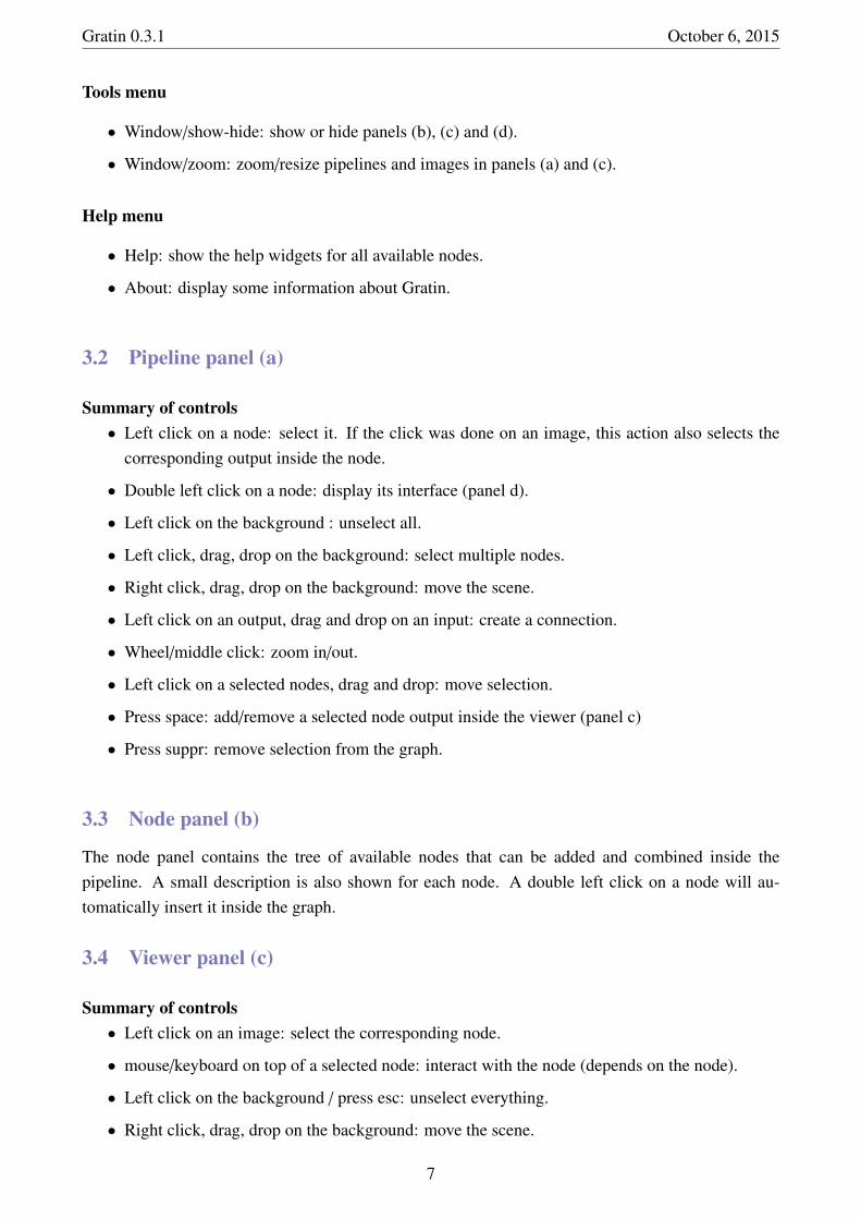
Figure 2: Each node interface is displayed as a list of widgets in the panel d.
The panel d contains a list of node interfaces opened by the user (via a double click on a node), asshown in Figure 22. Each widget thus contains parameters specific to each node as well as 3 buttons(as shown in the blue square):
• a help button (showing a small widget containing the documentation of this particular node),
• a detach button (detach the window - useful when programming inside the interface),
• a close button that removes this interface from the list (simply double-click again on the nodeto show it again).
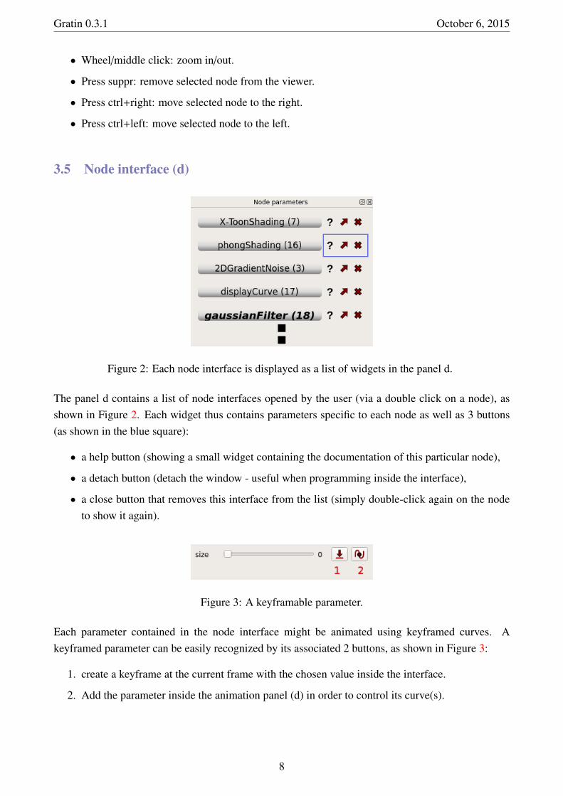
Figure 3: A keyframable parameter.
Each parameter contained in the node interface might be animated using keyframed curves. Akeyframed parameter can be easily recognized by its associated 2 buttons, as shown in Figure 33:
1. create a keyframe at the current frame with the chosen value inside the interface.
2. Add the parameter inside the animation panel (d) in order to control its curve(s).
8
Gratin 0.3.1 October 6, 2015
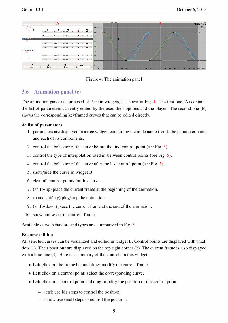
Figure 4: The animation panel
3.6 Animation panel (e)
The animation panel is composed of 2 main widgets, as shown in Fig. 44. The first one (A) containsthe list of parameters currently edited by the user, their options and the player. The second one (B)shows the corresponding keyframed curves that can be edited directly.
A: list of parameters1. parameters are displayed in a tree widget, containing the node name (root), the parameter name
and each of its components.
2. control the behavior of the curve before the first control point (see Fig. 55).
3. control the type of interpolation used in-between control points (see Fig. 55).
4. control the behavior of the curve after the last control point (see Fig. 55).
5. show/hide the curve in widget B.
6. clear all control points for this curve.
7. (shift+up) place the current frame at the beginning of the animation.
8. (p and shift+p) play/stop the animation
9. (shift+down) place the current frame at the end of the animation.
10. show and select the current frame.
Available curve behaviors and types are summarized in Fig. 55.
B: curve editionAll selected curves can be visualized and edited in widget B. Control points are displayed with smalldots (1). Their positions are displayed on the top right corner (2). The current frame is also displayedwith a blue line (3). Here is a summary of the controls in this widget:
• Left click on the frame bar and drag: modify the current frame.
• Left click on a control point: select the corresponding curve.
• Left click on a control point and drag: modify the position of the control point.
– +ctrl: use big steps to control the position.
– +shift: use small steps to control the position.
9
Gratin 0.3.1 October 6, 2015
Constant Linear Repeat Offsetted MirroredL
inea
rSt
epSh
epar
dSp
line
Her
mite
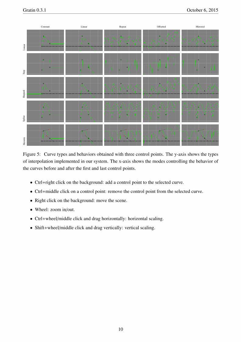
Figure 5: Curve types and behaviors obtained with three control points. The y-axis shows the typesof interpolation implemented in our system. The x-axis shows the modes controlling the behavior ofthe curves before and after the first and last control points.
• Ctrl+right click on the background: add a control point to the selected curve.
• Ctrl+middle click on a control point: remove the control point from the selected curve.
• Right click on the background: move the scene.
• Wheel: zoom in/out.
• Ctrl+wheel/middle click and drag horizontally: horizontal scaling.
• Shift+wheel/middle click and drag vertically: vertical scaling.
10
Gratin 0.3.1 October 6, 2015
4 Programming generic nodes
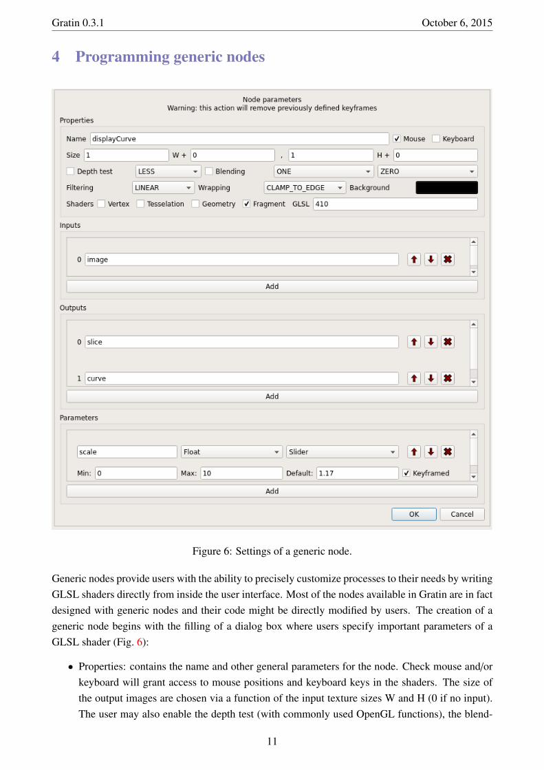
Figure 6: Settings of a generic node.
Generic nodes provide users with the ability to precisely customize processes to their needs by writingGLSL shaders directly from inside the user interface. Most of the nodes available in Gratin are in factdesigned with generic nodes and their code might be directly modified by users. The creation of ageneric node begins with the filling of a dialog box where users specify important parameters of aGLSL shader (Fig. 66):
• Properties: contains the name and other general parameters for the node. Check mouse and/orkeyboard will grant access to mouse positions and keyboard keys in the shaders. The size ofthe output images are chosen via a function of the input texture sizes W and H (0 if no input).The user may also enable the depth test (with commonly used OpenGL functions), the blend-
11

Gratin 0.3.1 October 6, 2015
ing, the filtering and the wrapping used for the output textures (see the OpenGL documentation- https://www.opengl.org/https://www.opengl.org/ - for more information on how these options will affect theresulting images). Finally, the user can decide which shaders to activate (vertex/tesselation/ge-ometry/fragment), choose the GLSL version and a default background color.
• Inputs/outputs: choose the number of input (resp. output) images and modify their names.Chosen names will be directly used inside the shaders.
• Parameters: add/remove necessary parameters. For each parameter, one may choose a name, atype (int/float/vec2/etc) and how it should appear in the node interface (slider/spin/etc). Min,max and default values should also be provided. Finally, checking the keyframed checkbox willallow the parameter to be controlled by keyframe curves.
Once the settings have been chosen, users may customize the node behavior by writing GLSL codeand observing results in real-time. Input and output names are used to automatically generate the headof the shaders. All the parameters are also available via generated uniform variables. In the following,we present the different types of generic nodes currently available in Gratin. For more informationabout how to program using GLSL, visit: https://www.opengl.org/documentation/glsl/https://www.opengl.org/documentation/glsl/.The provided pipeline samples also illustrate how each of these generic node has been used to producedifferent effects.
Remark: modifying the settings of a node will remove all previously defined keyframes forthis node
4.1 Generic image node
This node permits to analyze, manipulate and visualize input textures (e.g., colored images, g-buffers). As commonly done for image processing in OpenGL, a simple quad is drawn in the viewportso that input textures can be easily accessed and mapped to create outputs containing specific effects.This node may be used to create one-pass custom complex shaders (as in ShadertoyShadertoy for instance), tomix input images, to create various patterns and so on. Implementation-wise, user-specified GLSLversion, input and output texture names are automatically used to generate the header of the shader.By default, the fragment shader simply makes a copy of the first input texture.
4.2 Generic buffers and grid nodes
They let users apply any effect to 3D meshes by customizing vertex, tessellation, geometry andfragment shaders. The main difference between object and grid node types is that the former loads amesh in OBJ format, while the latter creates a planar grid. In the case of the grid node, tessellation ischosen by the user in the dedicated interface; vertices are then typically displaced according to inputGLSL code. As with other generic nodes, any number of textures might be provided as input (suchas color or normal maps for instance). Outputs are typically in the form of g-buffers or renderings forfurther 3D or 2D processing respectively. A trackball camera is associated to this node so that usersmay manipulate their object in the viewer panel. In both cases, mesh positions, normals, tangents
12
Gratin 0.3.1 October 6, 2015
and texture coordinates are directly sent as vertex attributes. Consequently, the header of the vertexshader is adapted to grant access to these attributes.
4.3 Generic splat node
This node permits to manipulate point sprites and is useful to control particles, visualizationsor even image warpings. The particularity here is to be able to modify splat sizes and locations(possibly using overlapping and blending) to obtain specific effects. The interface permits to controlthe number of rendered sprites, and their behavior is controlled through GLSL code. In practice, itworks by sending a set of point sprites to the GPU, with one splat per pixel by default. Shader headersfor the generic splat node contain the position of the splat (as an attribute in the vertex shader), as wellas uniform variables. The remainder of the shader can be freely modified.
4.4 Generic pyramid node
This node creates one or more mipmaped textures where one can control how each level is com-puted. It might be used for the creation of usual mipmaps, but also for multiscale analysis (Gaussianor Laplacian pyramids) or to compute global information such as the mean and variance of an inputimage. The shader header is automatically generated and contains variables such as the number oflevels and flags to know whether the top or bottom of the pyramid have been reached. In addition,the previously computed level of each input texture is automatically added to the GPU program as auniform sampler. Users thus only have to describe per-level operations in a specific order (top-downor bottom-up) in the GLSL code. The resulting pyramids are stored as mipmaps. Further connectednodes may thus easily access any texture level via GLSL built-in functions such as textureLod().
4.5 Generic ping-pong node
This node provides another useful feature commonly used in GPU programming to implementiterative processes. The same process is applied at each internal pass, and repeated a number of timesspecified by the user. Such a type of node may be used to iteratively accumulate or propagate someinformation in the output textures. In practice, it uses a pair of textures for internal multiple passes,with one texture being read and the other written on even passes, and the opposite on odd passes.However, this is not apparent to the user: we automatically generate a header that gives access to theresulting texture of the previous internal pass, as well as the current pass number. Note that such aping-pong architecture could not be created manually by connecting simpler nodes, since our graphis acyclic.
Remark: when opening a pipeline containing a ping-pong node, it will by default be initial-ized and run for the default number of passes. This might lead to important lags when eachpass is a time-consuming process.
13
Gratin 0.3.1 October 6, 2015
5 Pipeline samples
A good start for designing new pipelines is to have a look at and take inspiration from the providedsamples available in “data/pipes”. They describe how to use generic nodes and show how to easilyand quickly obtain multiple effects. This section presents the samples.
5.1 image-operators.gra
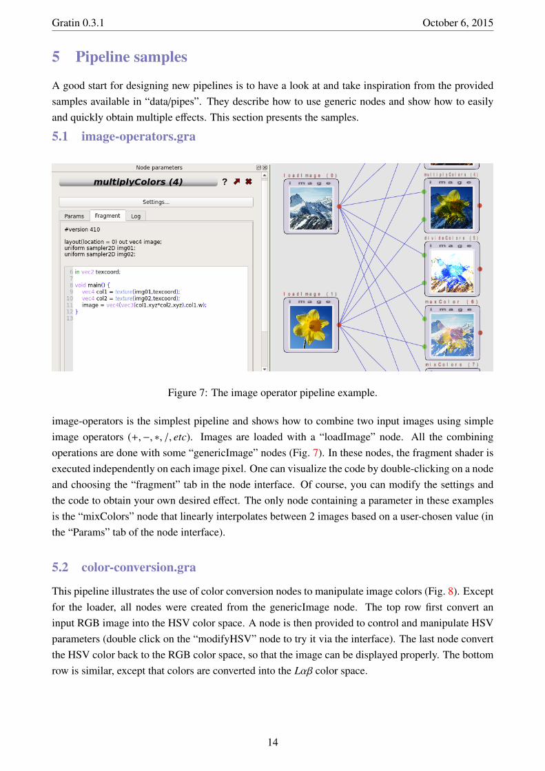
Figure 7: The image operator pipeline example.
image-operators is the simplest pipeline and shows how to combine two input images using simpleimage operators (+,−, ∗, /, etc). Images are loaded with a “loadImage” node. All the combiningoperations are done with some “genericImage” nodes (Fig. 77). In these nodes, the fragment shader isexecuted independently on each image pixel. One can visualize the code by double-clicking on a nodeand choosing the “fragment” tab in the node interface. Of course, you can modify the settings andthe code to obtain your own desired effect. The only node containing a parameter in these examplesis the “mixColors” node that linearly interpolates between 2 images based on a user-chosen value (inthe “Params” tab of the node interface).
5.2 color-conversion.gra
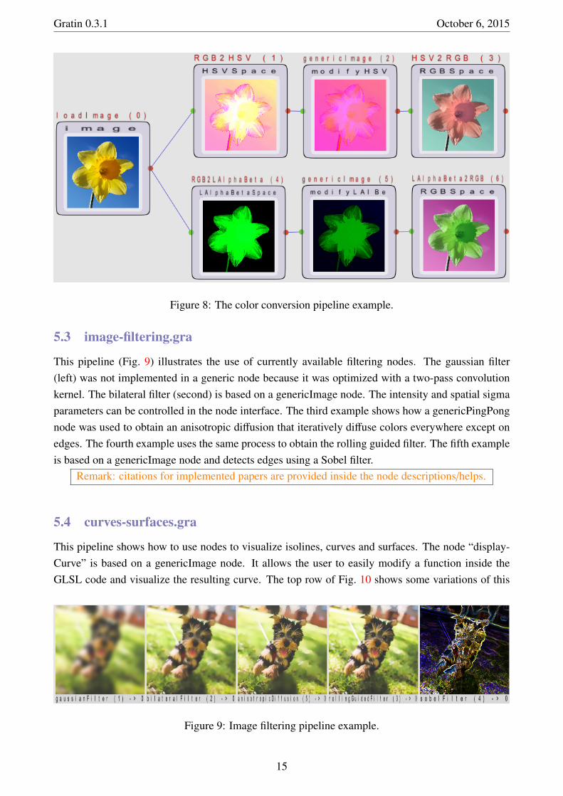
This pipeline illustrates the use of color conversion nodes to manipulate image colors (Fig. 88). Exceptfor the loader, all nodes were created from the genericImage node. The top row first convert aninput RGB image into the HSV color space. A node is then provided to control and manipulate HSVparameters (double click on the “modifyHSV” node to try it via the interface). The last node convertthe HSV color back to the RGB color space, so that the image can be displayed properly. The bottomrow is similar, except that colors are converted into the Lαβ color space.
14
Gratin 0.3.1 October 6, 2015
Figure 8: The color conversion pipeline example.
5.3 image-filtering.gra
This pipeline (Fig. 99) illustrates the use of currently available filtering nodes. The gaussian filter(left) was not implemented in a generic node because it was optimized with a two-pass convolutionkernel. The bilateral filter (second) is based on a genericImage node. The intensity and spatial sigmaparameters can be controlled in the node interface. The third example shows how a genericPingPongnode was used to obtain an anisotropic diffusion that iteratively diffuse colors everywhere except onedges. The fourth example uses the same process to obtain the rolling guided filter. The fifth exampleis based on a genericImage node and detects edges using a Sobel filter.
Remark: citations for implemented papers are provided inside the node descriptions/helps.
5.4 curves-surfaces.gra
This pipeline shows how to use nodes to visualize isolines, curves and surfaces. The node “display-Curve” is based on a genericImage node. It allows the user to easily modify a function inside theGLSL code and visualize the resulting curve. The top row of Fig. 1010 shows some variations of this
Figure 9: Image filtering pipeline example.
15
Gratin 0.3.1 October 6, 2015
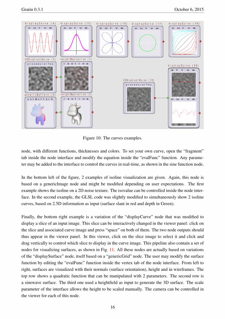
Figure 10: The curves examples.
node, with different functions, thicknesses and colors. To set your own curve, open the “fragment”tab inside the node interface and modify the equation inside the “evalFunc” function. Any parame-ter may be added to the interface to control the curves in real-time, as shown in the sine function node.
In the bottom left of the figure, 2 examples of isoline visualization are given. Again, this node isbased on a genericImage node and might be modified depending on user expectations. The firstexample shows the isoline on a 2D noise texture. The isovalue can be controlled inside the node inter-face. In the second example, the GLSL code was slightly modified to simultaneously show 2 isolinecurves, based on 2.5D information as input (surface slant in red and depth in Green).
Finally, the bottom right example is a variation of the “displayCurve” node that was modified todisplay a slice of an input image. This slice can be interactively changed in the viewer panel: click onthe slice and associated curve image and press “space” on both of them. The two node outputs shouldthus appear in the viewer panel. In this viewer, click on the slice image to select it and click anddrag vertically to control which slice to display in the curve image. This pipeline also contain a set ofnodes for visualizing surfaces, as shown in Fig. 1111. All these nodes are actually based on variationsof the “displaySurface” node, itself based on a “genericGrid” node. The user may modify the surfacefunction by editing the “evalFunc” function inside the vertex tab of the node interface. From left toright, surfaces are visualized with their normals (surface orientation), height and in wireframes. Thetop row shows a quadratic function that can be manipulated with 2 parameters. The second row isa sinewave surface. The third one used a heightfield as input to generate the 3D surface. The scaleparameter of the interface allows the height to be scaled manually. The camera can be controlled inthe viewer for each of this node.
16

Gratin 0.3.1 October 6, 2015
Figure 11: The surfaces examples.
5.5 flow-visualization.gra
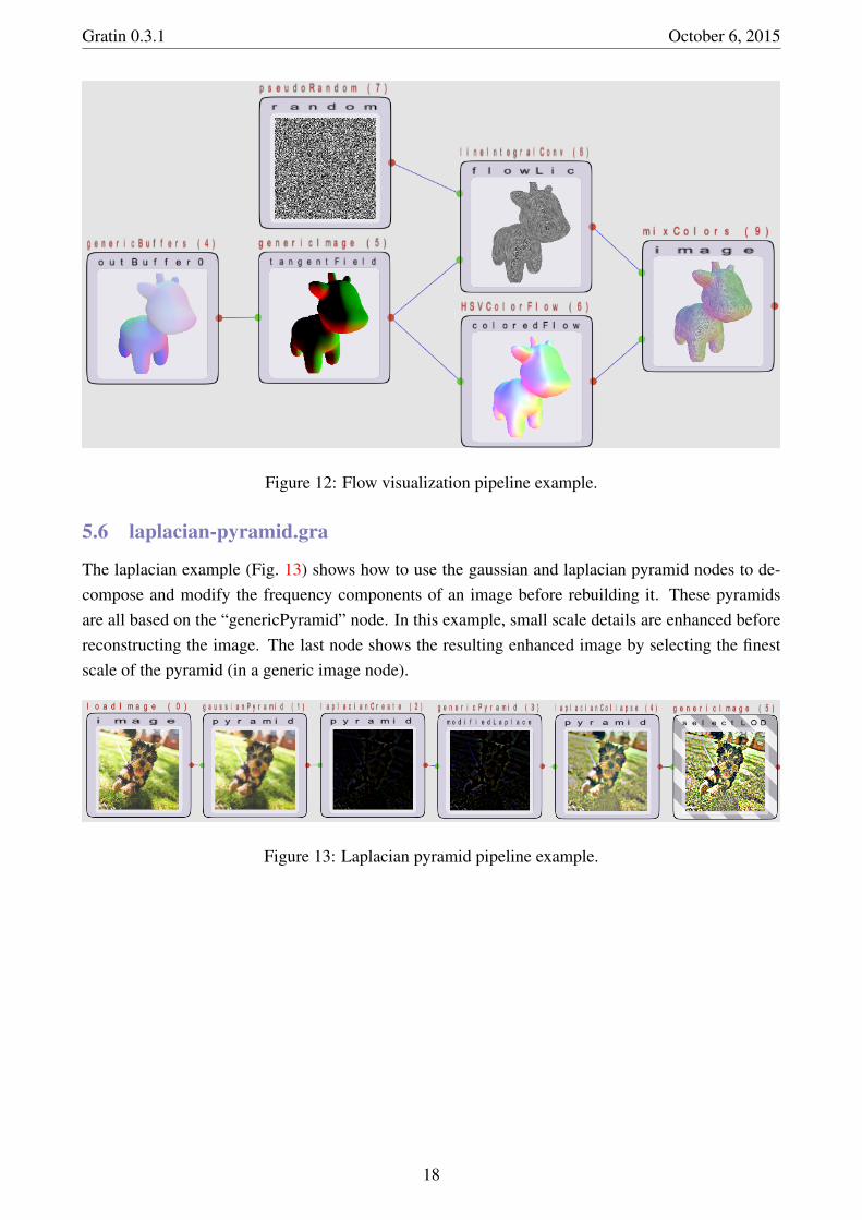
This pipeline (Fig 1212) illustrates the use of the “lineIntegralConv” and the “HSVColorFlow” nodes(based in generic image nodes) to visualize a flow field. In this example, the flow is obtained bycomputing the gradient flow of the surface. The line integral convolution (LIC) blurs a texture (thenoise in that case) in the direction of the flow. This process is commonly used to visualize flow field.The HSV color node has the same goal, but the input flow direction is visualized with different huesand magnitude is related to the color value. The last node on the right combines the flow to obtainan original visualization. The pipeline contains a second example where an image is abstracted byapplying a LIC, based on its gradient flow.
17
Gratin 0.3.1 October 6, 2015
Figure 12: Flow visualization pipeline example.
5.6 laplacian-pyramid.gra
The laplacian example (Fig. 1313) shows how to use the gaussian and laplacian pyramid nodes to de-compose and modify the frequency components of an image before rebuilding it. These pyramidsare all based on the “genericPyramid” node. In this example, small scale details are enhanced beforereconstructing the image. The last node shows the resulting enhanced image by selecting the finestscale of the pyramid (in a generic image node).
Figure 13: Laplacian pyramid pipeline example.
18

Gratin 0.3.1 October 6, 2015
5.7 global-values.gra
Figure 14: Global values pipeline example.
The pipeline shown in Fig. 1414 also makes use of pyramid nodes to compute global values on imagessuch as the minimum/maximum/mean/variance colors. This is shown on the left, where generic im-ages nodes are used to access the last levels of the pyramids and visualize the corresponding colors.On the right side, the mean and standard deviations are used to reshape the histogram of a sourceimage based on a target one (a simple example-based color transfer function).
5.8 histograms.gra
Figure 15: Histograms pipeline example.
Histograms (Fig. 1515) are based on generic splat nodes. The left side of the figure shows the originalnode as well as some variations that select only one particular channel to display. The geometryshader was slightly modified for this purpose. Histograms are obtained in real-time. Try to play withthe parameters of the “modifyHSV” node to visualize their effects. On the right side, a joint histogramis used to visualize the correlations between 2 rendered images.
19

Gratin 0.3.1 October 6, 2015
5.9 poisson-diffusion.gra
Figure 16: Diffusion pipeline example.
The pipeline shown in Fig. 1616 illustrates the use of the poisson diffusion node to reconstruct an imagefrom its gradients. On the left, 3 diffusions are computed (one for each channel) to compute the image.The “gradientDirichlet node” is based on a generic image node and computes the image gradient foreach channel, as well as some Dirichlet constraints on the borders (to avoid offset differences in theresult). The second example on the right shows how to use the poisson node to compute a laplaciandiffusion. In that case, the gradient is set to 0 everywhere. Only Dirichlet constraints are placed insidethe 2 black/white discs. The node then diffuses the data by minimizing the gradient. The positionsof the discs can be controlled in real-time in the viewer: click on the blackWhiteDiscs image, press“space” and modify the position of the discs with the mouse.
5.10 renderings.gra
The rendering pipeline (Fig. 1717) shows the available shading nodes on the left. They can all becontrolled via the mouse (for moving the light direction) or via some parameters inside the interface.The right example starts from a generic buffer node for loading the cow model, and uses the texturecoordinates as well as the tangents in order to perturb normal at the surface (normal-mapping tech-nique). The model texture is also loaded and combined with a simple shading to obtain the final resulton the right. Parameters for the normal perturbation, shading colors and textures might be modifiedinside the corresponding node interfaces.
20

Gratin 0.3.1 October 6, 2015
Figure 17: Renderings pipeline example.
5.11 displacement-mapping.gra
Figure 18: Displacement mapping pipeline example.
The displacement mapping technique (Fig. 1818) displaces mesh vertices based on an input heightmap. Here, the input texture also contains the associated normals, based on the gradient of a blurredcheckerboard texture. The displacement is applied on a sphere. The “disp” parameter inside theinterface of the displacement node controls how the sphere is deformed. “T” controls how the sphereshould be tesselated (how many triangles needed) via the tesselation shader to displace all the details.
5.12 animate.gra
The animation example illustrates basic animation behaviors. You will have to open the pipelineto follow the remainder of this section. The five nodes on the top row show a disc passing through4 control points, using five different interpolation types: linear, step, shepard, spline and hermite.The second row of nodes shows a rotated sunFlower illustrating the effect of the curve behavior on asmall number of control points: no behavior (all linear), constant, repeat, mirrored repeat and offsetedrepeat. Press the “p” key to start the animation and see the effects (press “shift+p” to stop it). Tocheck and modify the curves, click on the editing button of the parameter inside the interface of the
21
Gratin 0.3.1 October 6, 2015
node.
5.13 fourier-transform.gra
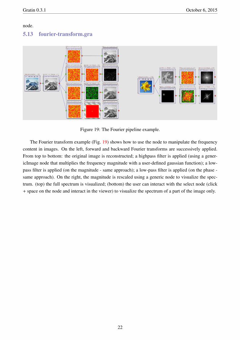
Figure 19: The Fourier pipeline example.
The Fourier transform example (Fig. 1919) shows how to use the node to manipulate the frequencycontent in images. On the left, forward and backward Fourier transforms are successively applied.From top to bottom: the original image is reconstructed; a highpass filter is applied (using a gener-icImage node that multiplies the frequency magnitude with a user-defined gaussian function); a low-pass filter is applied (on the magnitude - same approach); a low-pass filter is applied (on the phase -same approach). On the right, the magnitude is rescaled using a generic node to visualize the spec-trum. (top) the full spectrum is visualized; (bottom) the user can interact with the select node (click+ space on the node and interact in the viewer) to visualize the spectrum of a part of the image only.
22


![Eigen - TuxFamilydownloads.tuxfamily.org/eigen/eigen_aristote_may_2013.pdf · Eigen a c++ linear algebra library Gaël Guennebaud [] Séminaire Aristote – 15 May 2013](https://static.documents.pub/doc/80x56/5b9c930009d3f2f6368cd5a7/eigen-eigen-a-c-linear-algebra-library-gael-guennebaud-seminaire-aristote.jpg)