GRAVITATIONAL WAVES FROM BINARY NEUTRON

STARS AND TEST PARTICLE INSPIRALS INTO

BLACK HOLES

A Dissertation

Presented to the Faculty of the Graduate School

of Cornell University

in Partial Fulfillment of the Requirements for the Degree of

Doctor of Philosophy

by

Tanja Petra Hinderer

August 2008

GRAVITATIONAL WAVES FROM BINARY NEUTRON STARS AND TEST

PARTICLE INSPIRALS INTO BLACK HOLES

Tanja Petra Hinderer, Ph.D.

Cornell University 2008

As ground-based gravitational wave detectors are searching for gravitational waves

at their design sensitivity and plans for future space-based detectors are underway,

it is important to have accurate theoretical models of the expected gravitational

waves to be able to detect potential signals and extract information from the mea-

sured data. This thesis contains work on developing theoretical tools for modeling

the expected gravitational waves from two different classes of sources, which are

key targets for current and future gravitational wave detectors. The work is based

on four papers in collaboration with Eanna Flanagan. (i) We show that ground-

based gravitational wave detectors may be able to constrain the nuclear equation

of state using the early, relatively clean portion of the signal of detected neutron

star neutron star inspirals.

(ii) The second class of gravitational wave source we consider are radiation - re-

action driven inspirals of test particles into much more massive black holes. Chap-

ter 5 contains our work on developing a rigorous formalism based on two-timescale

expansions for treating the evolving orbit. Our results provide a clarification of the

existing prescription for computing the leading order orbital motion and resolve

the difficulties with previous approaches for going beyond leading order.

(iii) In Chapter 6, we analyze the effect of gravitational radiation reaction on

generic orbits around a body with an axisymmetric mass quadrupole moment Q

to linear order in Q, to linear order in the mass ratio and in the weak-field limit.

In addition we consider a system of two point masses where one body has a single

mass multipole or current multipole. We show that within our approximations the

motion is not integrable (except for the cases of spin and mass quadrupole).

(iv) Chapter 7 gives an alternative derivation of the result of Sago for an explicit

expression for the time-averaged rate of change of the Carter constant (a third

constant of geodesic motion around a rotating black hole in addition to energy

and axial angular momentum) in the adiabatic limit which is formulated in terms

of sums over modes and can be used for numerically computing leading order

waveforms.

BIOGRAPHICAL SKETCH

Tanja obtained the high school diploma “Abitur” from the Main-Taunus-Schule in

Hofheim, Germany and the BA from the University of Colorado at Boulder. She

went to Cornell University for her graduate studies, where she worked with Eanna

Flanagan.

iii

ACKNOWLEDGEMENTS

I thank Eanna Flanagan for being a superb adviser. With his enthusiasm about

science, his ability to communicate and present physics in a clear and well - or-

ganized way, his friendliness and willingness to take the time to provide extra

explanations, discussions, help and advice, he has taught me a lot about how to

be a better scientist and has made working with him a great experience.

I thank my family for all their love, support and encouragement.

I thank everyone I met, students, faculty, postdocs, and staff for many interest-

ing conversations, valuable discussions, fun experiences and educational lectures,

and for their friendship and support.

I gratefully acknowledge support from the John and David Boochever Prize

Fellowship in Theoretical Physics at Cornell.

iv

TABLE OF CONTENTS

Biographical Sketch . . . . . . . . . . . . . . . . . . . . . . . . . . . . . . iiiAcknowledgements . . . . . . . . . . . . . . . . . . . . . . . . . . . . . . ivTable of Contents . . . . . . . . . . . . . . . . . . . . . . . . . . . . . . . vList of Tables . . . . . . . . . . . . . . . . . . . . . . . . . . . . . . . . . ixList of Figures . . . . . . . . . . . . . . . . . . . . . . . . . . . . . . . . . x

1 Introduction 11.1 Gravitational Wave Astronomy . . . . . . . . . . . . . . . . . . . . 1

1.1.1 Gravitational Waves . . . . . . . . . . . . . . . . . . . . . . 11.1.2 Benefits of Theoretical Modeling of Gravitational Wave

Sources . . . . . . . . . . . . . . . . . . . . . . . . . . . . . 121.2 Neutron stars . . . . . . . . . . . . . . . . . . . . . . . . . . . . . . 13

1.2.1 Potential gravitational wave measurements . . . . . . . . . . 191.3 Extreme mass ratio inspirals . . . . . . . . . . . . . . . . . . . . . . 24

1.3.1 Modelling extreme mass ratio inspirals . . . . . . . . . . . . 27

2 Constraining neutron star tidal Love numbers with gravitationalwave detectors 332.1 Background and Motivation . . . . . . . . . . . . . . . . . . . . . . 332.2 Tidal interactions in compact binaries . . . . . . . . . . . . . . . . . 352.3 Tidal Love number . . . . . . . . . . . . . . . . . . . . . . . . . . . 362.4 Effect on gravitational wave signal . . . . . . . . . . . . . . . . . . 372.5 Accuracy of Model . . . . . . . . . . . . . . . . . . . . . . . . . . . 412.6 Measuring the Love Number . . . . . . . . . . . . . . . . . . . . . 43

3 Tidal Love numbers of neutron stars 463.1 Introduction and Motivation . . . . . . . . . . . . . . . . . . . . . . 463.2 Definition of the Love number . . . . . . . . . . . . . . . . . . . . . 493.3 Calculation of the Love number . . . . . . . . . . . . . . . . . . . . 52

3.3.1 Equilibrium configuration . . . . . . . . . . . . . . . . . . . 523.3.2 Static linearized perturbations due to an external tidal field 523.3.3 Newtonian limit . . . . . . . . . . . . . . . . . . . . . . . . . 55

3.4 Results and Discussion . . . . . . . . . . . . . . . . . . . . . . . . . 55

4 Two timescale analysis of extreme mass ratio inspirals in Kerr. I.Orbital Motion 604.1 Introduction and Summary . . . . . . . . . . . . . . . . . . . . . . . 61

4.1.1 Background and Motivation . . . . . . . . . . . . . . . . . . 614.1.2 Methods of computing orbital motion and waveforms . . . . 644.1.3 The two timescale expansion method . . . . . . . . . . . . . 694.1.4 Orbital Motion . . . . . . . . . . . . . . . . . . . . . . . . . 714.1.5 Two timescale expansion of the Einstein equations and adi-

abatic waveforms . . . . . . . . . . . . . . . . . . . . . . . . 75

v

4.1.6 Organization of this Paper . . . . . . . . . . . . . . . . . . . 794.1.7 Notation and Conventions . . . . . . . . . . . . . . . . . . . 79

4.2 Extreme Mass Ratio Inspirals in Kerr formulated using action-anglevariables . . . . . . . . . . . . . . . . . . . . . . . . . . . . . . . . . 804.2.1 Review of action-angle variables in geometric Hamiltonian

mechanics . . . . . . . . . . . . . . . . . . . . . . . . . . . . 814.2.2 Generalized action-angle variables for non-compact level sets 854.2.3 Application to bound geodesic motion in Kerr . . . . . . . . 874.2.4 Explicit expressions in terms of Boyer-Lindquist coordinates 904.2.5 Application to slow inspiral motion in Kerr . . . . . . . . . . 944.2.6 Rescaled variables and incorporation of backreaction on the

black hole . . . . . . . . . . . . . . . . . . . . . . . . . . . . 974.2.7 Conservative and dissipative pieces of the forcing terms . . . 105

4.3 A general weakly perturbed dynamical system . . . . . . . . . . . . 1094.4 Systems with a single degree of freedom . . . . . . . . . . . . . . . 112

4.4.1 Overview . . . . . . . . . . . . . . . . . . . . . . . . . . . . 1124.4.2 Fourier expansions of the perturbing forces . . . . . . . . . . 1134.4.3 Two timescale ansatz for the solution . . . . . . . . . . . . . 1154.4.4 Results of the two-timescale analysis . . . . . . . . . . . . . 1174.4.5 Derivation . . . . . . . . . . . . . . . . . . . . . . . . . . . . 122

4.5 Systems with several degrees of freedom subject to non-resonantforcing . . . . . . . . . . . . . . . . . . . . . . . . . . . . . . . . . . 1284.5.1 Overview . . . . . . . . . . . . . . . . . . . . . . . . . . . . 1284.5.2 Fourier expansions of perturbing forces . . . . . . . . . . . . 1294.5.3 The no-resonance assumption . . . . . . . . . . . . . . . . . 1314.5.4 Two timescale ansatz for the solution . . . . . . . . . . . . . 1334.5.5 Results of the two-timescale analysis . . . . . . . . . . . . . 1354.5.6 Derivation . . . . . . . . . . . . . . . . . . . . . . . . . . . . 141

4.6 Numerical Integration of an illustrative example . . . . . . . . . . . 1504.7 Discussion . . . . . . . . . . . . . . . . . . . . . . . . . . . . . . . . 153

4.7.1 Consistency and uniqueness of approximation scheme . . . . 1534.7.2 Effects of conservative and dissipative pieces of the self force 1554.7.3 The radiative approximation . . . . . . . . . . . . . . . . . . 1574.7.4 Utility of adiabatic approximation for detection of gravita-

tional wave signals . . . . . . . . . . . . . . . . . . . . . . . 1604.8 Conclusions . . . . . . . . . . . . . . . . . . . . . . . . . . . . . . . 165

4.8.1 Acknowledgements . . . . . . . . . . . . . . . . . . . . . . . 1664.9 Appendix: Explicit expressions for the coefficients in the action-

angle equations of motion . . . . . . . . . . . . . . . . . . . . . . . 1664.10 Appendix: Comparison with treatment of Kevorkian and Cole . . . 168

5 Evolution of the Carter constant for inspirals into a black hole:effect of the black hole quadrupole 1695.1 Introduction and summary . . . . . . . . . . . . . . . . . . . . . . . 170

vi

5.2 Effect of an axisymmetric mass quadrupole on the conservative or-bital dynamics . . . . . . . . . . . . . . . . . . . . . . . . . . . . . . 1775.2.1 Conservative orbital dynamics in a Boyer-Lindquist-like co-

ordinate system . . . . . . . . . . . . . . . . . . . . . . . . . 1785.2.2 Effects linear in spin on the conservative orbital dynamics . 181

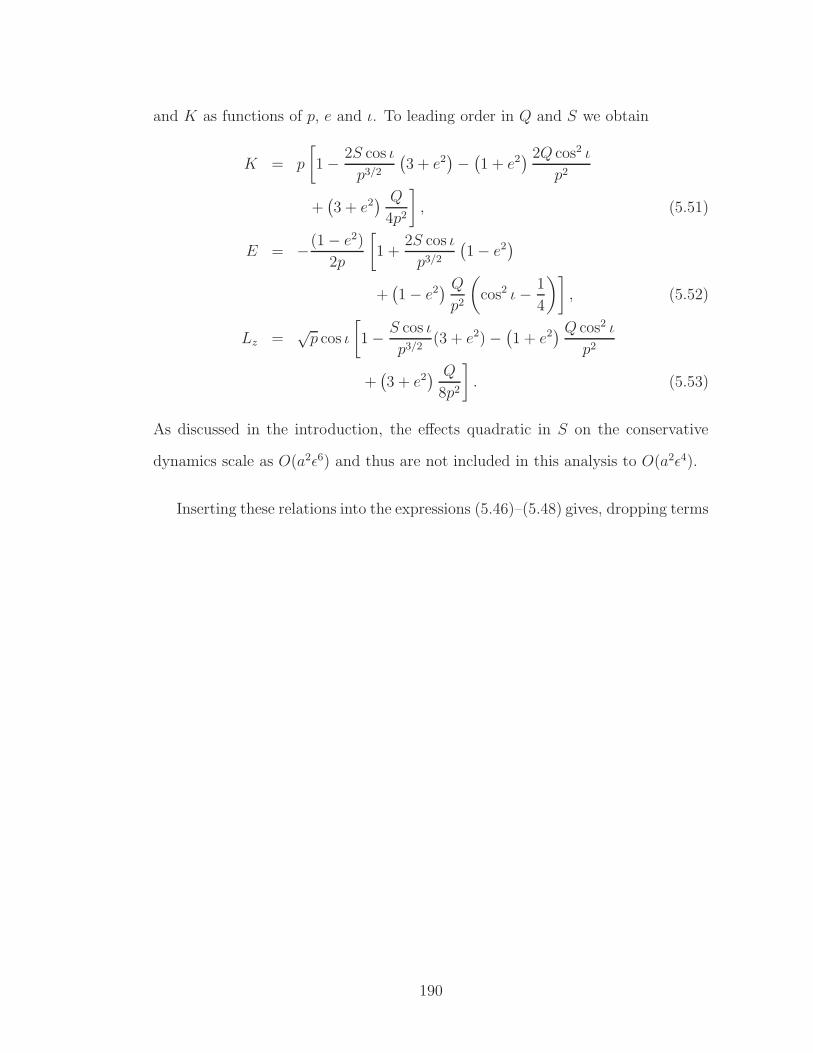
5.3 Effects linear in quadrupole and quadratic in spin on the evolutionof the constants of motion . . . . . . . . . . . . . . . . . . . . . . . 1825.3.1 Evaluation of the radiation reaction force . . . . . . . . . . . 1825.3.2 Instantaneous fluxes . . . . . . . . . . . . . . . . . . . . . . 1865.3.3 Alternative set of constants of the motion . . . . . . . . . . 1895.3.4 Time averaged fluxes . . . . . . . . . . . . . . . . . . . . . . 193

5.4 Application to black holes . . . . . . . . . . . . . . . . . . . . . . . 1965.4.1 Qualitative discussion of results . . . . . . . . . . . . . . . . 1965.4.2 Comparison with previous results . . . . . . . . . . . . . . . 196

5.5 Non-existence of a Carter-type constant for higher multipoles . . . . 1995.5.1 Separability analysis . . . . . . . . . . . . . . . . . . . . . . 2005.5.2 Derivation of non-existence of additional constants of the

motion . . . . . . . . . . . . . . . . . . . . . . . . . . . . . . 2055.6 Conclusion . . . . . . . . . . . . . . . . . . . . . . . . . . . . . . . . 2145.7 Acknowledgments . . . . . . . . . . . . . . . . . . . . . . . . . . . . 2155.8 Appendix: Time variation of quadrupole: order of magnitude esti-

mates . . . . . . . . . . . . . . . . . . . . . . . . . . . . . . . . . . 2155.8.1 Estimate of the scaling for the nonspinning case . . . . . . . 2165.8.2 Estimate of the scaling for the spinning case . . . . . . . . . 2165.8.3 Application to Kerr inspirals . . . . . . . . . . . . . . . . . . 217

5.9 Appendix: Computation of time averaged fluxes . . . . . . . . . . . 2185.9.1 Averaging method that parallels fully relativistic averaging . 2185.9.2 Averaging method using the explicit parameterization of

Newtonian orbits . . . . . . . . . . . . . . . . . . . . . . . . 222

6 Carter constant evolution in the adiabatic regime 2256.1 Introduction . . . . . . . . . . . . . . . . . . . . . . . . . . . . . . . 2256.2 The Kerr spacetime . . . . . . . . . . . . . . . . . . . . . . . . . . . 228

6.2.1 Teukolsky perturbation formalism . . . . . . . . . . . . . . . 2286.2.2 Boyer-Lindquist coordinates . . . . . . . . . . . . . . . . . . 234

6.3 Vacuum equations . . . . . . . . . . . . . . . . . . . . . . . . . . . 2406.3.1 Separation of variables . . . . . . . . . . . . . . . . . . . . . 2406.3.2 Basis of modes . . . . . . . . . . . . . . . . . . . . . . . . . 2436.3.3 “in”, “up”, “out”, and “down” modes . . . . . . . . . . . . . 2456.3.4 Relations between the scattering and transmission coefficients2496.3.5 Mode expansion of the potential for the metric perturbation 254

6.4 Construction of the Green’s functions for the Teukolsky variables . 2576.4.1 Formula for the retarded Green’s function . . . . . . . . . . 2576.4.2 Derivation . . . . . . . . . . . . . . . . . . . . . . . . . . . . 258

vii

6.4.3 Construction of the radiative Green’s function for theTeukolsky variables . . . . . . . . . . . . . . . . . . . . . . . 264

6.4.4 The inhomogeneous potentials . . . . . . . . . . . . . . . . . 2686.4.5 Harmonic decomposition of the amplitudes . . . . . . . . . . 2706.4.6 Derivation . . . . . . . . . . . . . . . . . . . . . . . . . . . . 2746.4.7 Expressions for the time derivatives of the constants of motion277

6.5 Comparison of the notation to other conventions . . . . . . . . . . . 2876.6 Two-timescale method . . . . . . . . . . . . . . . . . . . . . . . . . 288

6.6.1 Analysis of the O(ε) Einstein equation . . . . . . . . . . . . 2886.7 Appendix: Sketch of the derivation of the Teukolsky-Starobinsky

identities . . . . . . . . . . . . . . . . . . . . . . . . . . . . . . . . . 306

Bibliography 310

viii

LIST OF TABLES

3.1 Relativistic Love numbers k2 . . . . . . . . . . . . . . . . . . . . . 583.2 Estimated neutron star parameters from X-ray observations from

Webb and Barrett and Ozel used to generate the figure. . . . . . . 59

ix

LIST OF FIGURES

1.1 The effect of a gravitational wave passing down the z−axis on aring of test particles is an oscillatory stretching and squeezing ofspace along orthogonal axes. . . . . . . . . . . . . . . . . . . . . . 2

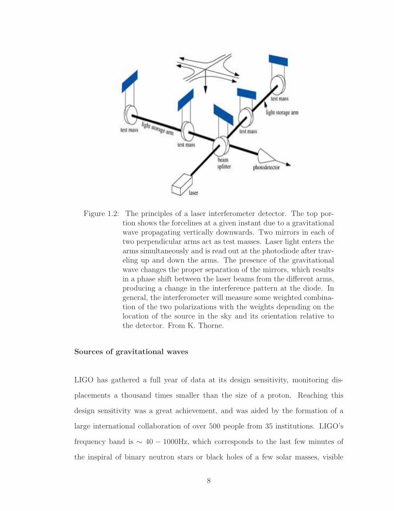
1.2 The principles of a laser interferometer detector. The top portionshows the forcelines at a given instant due to a gravitational wavepropagating vertically downwards. Two mirrors in each of two per-pendicular arms act as test masses. Laser light enters the armssimultaneously and is read out at the photodiode after travelingup and down the arms. The presence of the gravitational wavechanges the proper separation of the mirrors, which results in aphase shift between the laser beams from the different arms, pro-ducing a change in the interference pattern at the diode. In general,the interferometer will measure some weighted combination of thetwo polarizations with the weights depending on the location of thesource in the sky and its orientation relative to the detector. FromK. Thorne. . . . . . . . . . . . . . . . . . . . . . . . . . . . . . . . 8

1.3 The noise curves hrms(f) =√

fSh(f) for LIGO I and LIGO II areshown in red (thin lines). The thicker blue line shows the signalhc(f) for two 1.4M⊙ neutron stars at a distance of 200Mpc. Thesignal terminates at the innermost stable circular orbit, where thegravitational wave frequency (twice the orbital frequency) is fisco ∼850Hz assuming the stars have R = 10km, and pressure-densityrelation p ∝ ρ2. From Racine and Flanagan, 2006. . . . . . . . . . 21

1.4 The form of an expected “chirp” signal from an inspiralling binaryas a function of time. Both the frequency and amplitude increaseas the inspiral progresses. From K. Thorne. . . . . . . . . . . . . . 21

2.1 [Top] The solid lines bracket the range of Love numbers λ for fullyrelativistic polytropic neutron star models of mass m with surfaceredshift z = 0.35, assuming a range of 0.3 ≤ n ≤ 1.2 for the adia-batic index n. The top scale gives the radius R for these relativisticmodels. The dashed lines are corresponding Newtonian values forstars of radius R. [Bottom] Upper bound (horizontal line) on theweighted average λ of the two Love numbers obtainable with LIGOII for a binary inspiral signal at distance of 50 Mpc, for two non-spinning, 1.4M⊙ neutron stars, using only data in the frequencyband f < 400 Hz. The curved lines are the actual values of λ forrelativistic polytropes with n = 0.5 (dashed line) and n = 1.0 (solidline). . . . . . . . . . . . . . . . . . . . . . . . . . . . . . . . . . . 38

x

2.2 [Top] Analytic approximation (2.10) to the tidal perturbation tothe gravitational wave phase for two identical 1.4M⊙ neutron starsof radius R = 15 km, modeled as n = 1.0 polytropes, as a functionof gravitational wave frequency f . [Bottom] A comparison of differ-ent approximations to the tidal phase perturbation: the numericalsolution (lower dashed, green curve) to the system (2.6), and theadiabatic analytic approximation (2.9) (upper dashed, blue), bothin the limit (2.11) and divided by the leading order approximation(2.10). . . . . . . . . . . . . . . . . . . . . . . . . . . . . . . . . . . 41

3.1 The relativistic Love numbers k2. . . . . . . . . . . . . . . . . . . 563.2 The difference in percent between the relativistic dimensionless

Love numbers k2 and the Newtonian values kN2 . . . . . . . . . . . . 563.3 The range of Love numbers for the estimated NS parameters from

X-ray observations. Top to bottom sheets: EXO0748-676, ωCen,M 13, NGC 2808. For an inspiral of two 1.4M⊙ NSs at a distanceof 50 Mpc, LIGO II detectors will be able to constrain λ to λ ≤20.1 × 1036g cm2s2 with 90% confidence. . . . . . . . . . . . . . . . 57

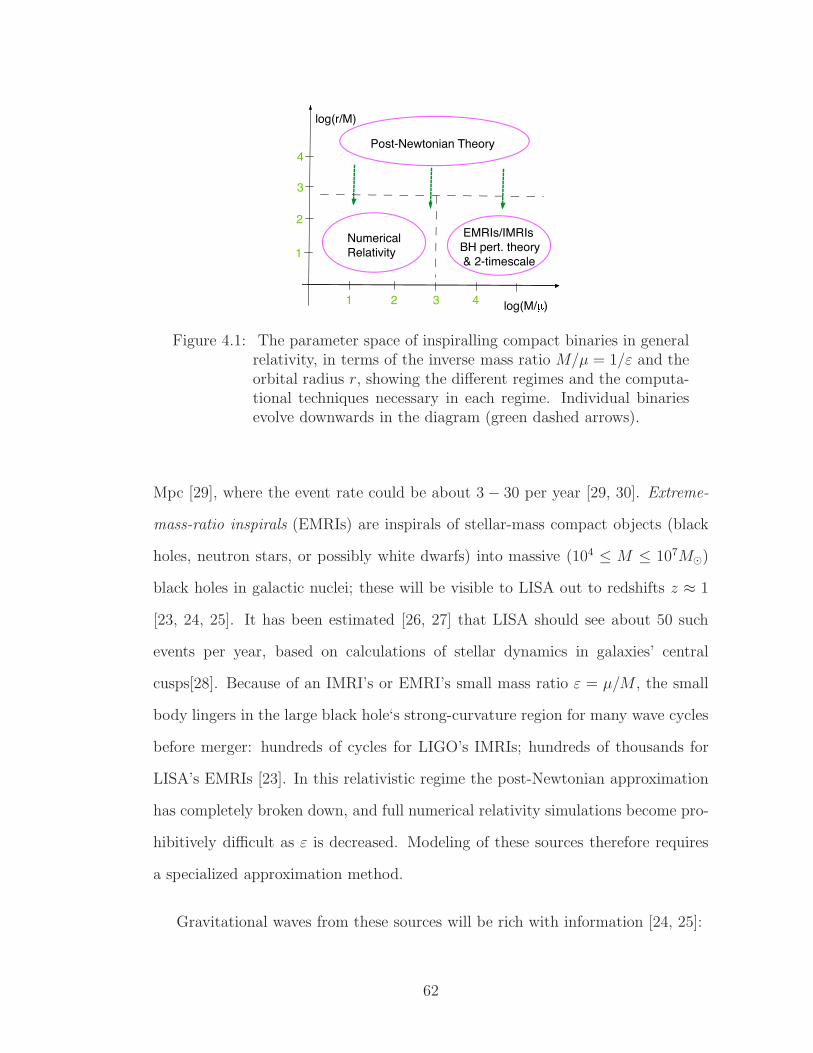
4.1 The parameter space of inspiralling compact binaries in general rel-ativity, in terms of the inverse mass ratioM/µ = 1/ε and the orbitalradius r, showing the different regimes and the computational tech-niques necessary in each regime. Individual binaries evolve down-wards in the diagram (green dashed arrows). . . . . . . . . . . . . 62

4.2 The exact numerical solution of the system of equations (4.233).After a time ∼ 1/ε, the action variable J is O(1), while the anglevariable q is O(1/ε). . . . . . . . . . . . . . . . . . . . . . . . . . . 151

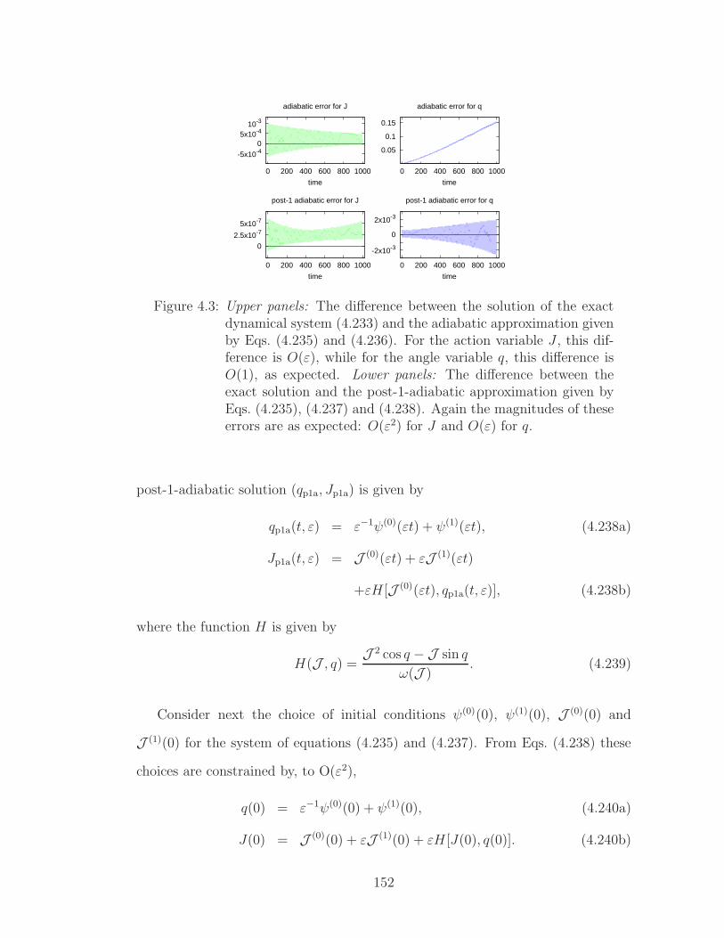
4.3 Upper panels: The difference between the solution of the exact dy-namical system (4.233) and the adiabatic approximation given byEqs. (4.235) and (4.236). For the action variable J , this differenceis O(ε), while for the angle variable q, this difference is O(1), asexpected. Lower panels: The difference between the exact solu-tion and the post-1-adiabatic approximation given by Eqs. (4.235),(4.237) and (4.238). Again the magnitudes of these errors are asexpected: O(ε2) for J and O(ε) for q. . . . . . . . . . . . . . . . . 152

xi

4.4 The maximum orbital phase error in cycles, δN = δφ/(2π), in-curred in the radiative approximation during the last year of inspi-ral, as a function of the mass M6 of the central black hole in units of106M⊙, the mass µ10 of the small object in units of 10M⊙, and theeccentricity e of the system at the start of the final year of inspi-ral. The exact and radiative inspirals are chosen to line up at sometime tm during the final year, and the value of tm is chosen to min-imize the phase error. The initial data at time tm for the radiativeevolution is slightly different to that used for the exact evolution inorder that the secular pieces of the two evolutions initially coincide;this is the “time-averaged” initial data prescription of Pound andPoisson. All evolutions are computed using the hybrid equationsof motion of Kidder, Will and Wiseman in the osculating-elementform given by Pound and Poisson. . . . . . . . . . . . . . . . . . . 163

6.1 An illustration of the various types of modes in black hole space-times. Here J − denotes past null infinity, J + future null infin-ity, E− the past event horizon, and E+ the future event horizon.The four panels give the behavior of the four different modes “in”,“out”, “up” or “down” as indicated. A zero indicates the modevanishes at the indicated boundary. Two arrows indicates that themode consists of a mixture of ingoing and outgoing radiation atthat boundary. Two arrows with an “OR” means that the mode iseither purely ingoing or purely outgoing at that boundary, depend-ing on the relative sign of pmω and ω. The “in” modes vanish on thepast event horizon, and the “up” modes vanish on past null infin-ity. Thus the “in” and “up” modes together form a complete basisof modes. Similarly the “down” and “out” modes together form acomplete basis of modes. From Drasco, Flanagan and Hughes, 2005. 246

xii

CHAPTER 1

INTRODUCTION

1.1 Gravitational Wave Astronomy

To introduce the work in this thesis on theoretical tools for analyzing sources of

gravitational waves, we first give some well - known background material that can

be found in textbooks such as [1, 2].

1.1.1 Gravitational Waves

Almost a century ago, Einstein’s theory of general relativity radically changed

the notion of space and time: they are not just the stage upon which events

occur; instead spacetime is a dynamic entity which curves, expands and contracts

around matter and energy. The theory of general relativity predicts the existence of

transverse distortions of spacetime curvature, called gravitational waves, which, as

a consequence of causality, propagate at the speed of light (since information about

the changing gravitational field cannot reach distant observers faster than light).

However, scientists at the time concluded that gravitational radiation would not

be observable because it is produced only in extremely small quantities in everyday

and atomic processes. For example, the probability for an electron transition of

energy E ∼ 1eV between two atomic states by gravitational radiation rather than

electromagnetic radiation is of order the ratio of the square of the dimensionless

”coupling constants” for the gravitational and electromagnetic interactions [1]:

∼ (G/c5)(E2/~)/(e2/~c) ∼ 10−54, which reflects how weakly gravitational waves

interact with matter fields.

1

Figure 1.1: The effect of a gravitational wave passing down the z−axis ona ring of test particles is an oscillatory stretching and squeezingof space along orthogonal axes.

Nevertheless, in the 1960’s, scientists started to look for gravitational radiation

emitted coherently by the bulk motion of matter and energy in violent astrophysical

processes, for which the prospects of detection were better. One characteristic of a

gravitational waves’ spacetime warpage is an oscillatory stretching and squeezing of

space. Test particles in the presence of a passing gravitational wave will experience

gravitational tidal forces that alternately stretch and squeeze along orthogonal axes

in the plane perpendicular to the direction of propagation. The tidal deformations

preserve the area enclosed by a ring of test particles, so a measure of the strength is

the relative fractional deformation, or dimensionless strain amplitude, h = 2∆L/L,

where L is the length and ∆L is the change in length. Just as electromagnetic

waves, gravitational waves have two polarizations, commonly called h+ and h×,

however, they are rotated by 45o with respect to one another as opposed to 90o

because they correspond to a spin-2 field. The effect of the two polarization fields

on a ring of test particles is illustrated in Fig. (1.1).

The strain amplitude will typically be very small when waves from astrophys-

ical sources reach the Earth. In the leading order approximation at large dis-

2

tances from the source, gravitational waves are produced by the time-changing

mass quadrupole moment Qij(t) ≡∫

d3xρ(x, t)[xixj − x2δij/3], where ρ is the

density, since monopole waves would violate mass-energy conservation and dipole

waves would violate momentum conservation. The dimensionless strain is of order

[1]:

h ∼ G

c41

r

d2

dt2Q, (1.1)

where r is the distance to source. The tiny factor of (G/c4) = 8× 10−45s2kg−1m−1

reflects the fact that gravity is the weakest of the fundamental interactions. Only

sources which are compact and highly dynamical can compensate for this factor.

But even for large masses undergoing rapid variation, the expected strain from

typical sources scientists hope to detect on earth is still very small:

h ∼ 10−22

(

M

2.8M⊙

)5/3(0.01s

P

)2/3(100Mpc

r

)

, (1.2)

where the numbers correspond to typical binary neutron stars that are spiralling

together with an orbital period P , and the symbol M⊙ denotes the mass of the

Sun, ≈ 2 × 1030kg.

The gravitational waves from astrophysical sources have low frequencies

(10−18Hz - 103Hz) since the frequency is determined by the characteristic timescale

for the source, and we expect that events involving large astrophysical bodies

probably have timescales greater than a millisecond. Compare this to the high

frequency of order 1015Hz of visible light. For light, the wavelength is typically

much smaller than the size of its source, so it can form images; this is not possible

for gravitational waves whose wavelength is typically much larger than the size of

source. The information contained in the waves is encoded in the time varying

amplitudes of the two polarizations h+(t) and h×(t), as for stereophonic sound.

Gravitons are typically phase coherent, emitted by bulk mass motion, rather than

3

phase incoherent superpositions of waves from atoms, molecules, and particles.

Gravitational waves have not yet been directly detected but compelling indirect

evidence for their existence was the basis of the 1993 Nobel Prize in physics. Hulse

and Taylor had monitored the orbital motion of the binary pulsar PSR1913+16

(two neutron stars orbiting each other) for 18 years from the Doppler shifting

of radio signals emitted by the pulsar. General relativity predicts that gravita-

tional radiation carries off energy and angular momentum and as a result the orbit

shrinks. The prediction for the inspiral rate of 3mm per orbit agrees to ∼ 0.1% with

the observation, within the experimental uncertainty [3]. Today, astronomers are

performing similar measurements on five more such double neutron star systems

that have been discovered since then [4].

Scientists are now trying to detect gravitational waves directly, and to use them

as a tool for astronomy to study phenomena that are likely not visible electromag-

netically. Whereas electromagnetic signals from distant events are easily absorbed

and scattered (for example by dust), gravitational waves pass through essentially

unimpeded because they couple so weakly to matter.

The theoretical description of gravitational waves

We now discuss the regime in which the notion of “gravitational waves” makes

sense. Within finite regions of space, gravitational waves cannot be defined at

a fundamental level, one can only speak about time-varying gravitational fields.

Gravitational waves can only be approximately defined in local regions in the spe-

cial context when their wavelength λGW is much smaller than the characteristic

scale R of the background curvature. This is analogous to the surface of a grape-

fruit, which has an overall, roughly spherical background curvature and dimples

4

on small scales, analogous to the gravitational waves. For example, for ∼ 100Hz

waves, the wavelength is λGW ∼ 500km and on earth, the background curvature

is R ∼ 109km, so this will be a good approximation [1]. Mathematically, one can

describe gravitational radiation in this regime as approximately plane waves within

a small region of space and, to linear order, define the background quantities such

as the curvature and the distance rule to be the “coarse-grain ” average value over

lengthscales large compared to λGW but small compared to R. The leftover, fluctu-

ating pieces can be interpreted as effectively describing gravitational waves, which

can then be treated as any other matter source. A meaningful concept is then

the average energy density over spacetime volumes of dimensions larger than λGW

but much smaller than R, which must include the backreaction describing how the

wave produces background spacetime curvature due to the nonlinear interactions

with itself. Energy and momentum density cannot be localized at a point and are

not defined on lengthscales shorter than the wavelength. A plane wave propagating

in a flat background spacetime is completely described by its two dimensionless

polarization amplitudes h+ and h×. Taking the propagation direction to be along

the z−axis, one finds that the energy flux T tz in the gravitational wave is given by

T tz =1

16π

c3

G〈(∂th+)2 + (∂th×)2〉, (1.3)

where the angular brackets mean an average over several wavelengths. Assuming

that the wave varies as h+ = h cos(ωt− ωz), the energy flux is given by

T tz =π

4

c3

G2f 2h2 ≈ 1.5 × 10−3Wm−2

(

h

10−22

)2(f

1kHz

)2

, (1.4)

where the numbers are for a supernova in the Virgo cluster of galaxies. Note that

this flux is large by astronomical standards: it is comparable to the flux of reflected

sunlight from a full moon. However, most gravitons pass through a detector (like

neutrinos and unlike photons).

5

Interaction of gravitational waves with a detector

A simple way to see how the waves affect matter is to consider how two free particles

in empty space react to the wave. Gravitational waves cause the proper distance

between two freely falling particles to oscillate, even if the coordinate separation

is constant. Consider a freely falling test particle and define a coordinate system

that is chosen to be as nearly Newtonian as possible, i.e. distorted as little as

possible by the gravitational waves, so that coordinate displacements are the same

as proper separations to a good accuracy. In this coordinate system, consider

another nearby test particle and let Lj be the components of the separation vector

between the particles’ worldlines initially. In the approximation that L << λGW,

a passing gravitational wave will produce a relative acceleration given by [1]

d2Li

dt2=

1

2hTTij L

j , (1.5)

where the overdots indicate time derivatives and hTTij is a symmetric spatial tensor

which is transverse to the propagation direction and trace - free (the analog of

the vector potential in Lorentz gauge in electromagnetism) and has non - zero

components hxx = −hyy = h+(t − z) and hxy = hyx = h×(t − z) (for propagation

along the z - axis). It follows that the particles’ separation changes by and amount

δLi(t) =1

2hTTij (t)Lj , (1.6)

where δLi is the coordinate displacement produced by the passing wave.

Current interferometer detectors

The great challenge in detecting gravitational waves is the extraordinarily small

effect the waves produce on a detector. As discussed above, even waves from violent

6

astrophysical events have a very small amplitude when they reach the Earth, of

order h ∼ 10−21. For an object 1 m in length, this means that its ends would move

by 10−21m relative to one other. This distance is about a millionth of the width

of a proton. The most sensitive gravitational wave detectors today are Michelson-

type interferometers, such as LIGO, the Laser Interferometer Gravitational wave

Observatory with sites in Livingston, Louisiana and Hanford, Washington [5]. The

LIGO detectors are part of a network of similar detectors around the world, most

notably the French-Italian VIRGO, the British-German GEO, and the Japanese

TAMA detector [6]. The cartoon-version of the detectors is illustrated in Fig.

(1.2). Two mirrors, which act as test masses, hang far apart in a vacuum pipe

(4 or 2 km) forming one “arm”, and two more mirrors form a perpendicular arm.

A laser beam is split in two after passing through a beam splitter located at the

vertex of the perpendicular arms and each beam enters one of the arms. The light

bounces between the mirrors repeatedly before recombining at the beam splitter

and returning to the readout at the photodiode. A relative change in separation

∆L = δLx − δLy of the end mirrors and the beam splitter will produce a phase

shift of the laser beams δφ = (4π/λ)∆L, where λ is the wavelength of the laser,

which results in a change in the intensity at the photodiode.

The detector sensitivity is limited by frequency-dependent noise of various kinds:

For example, there are non-gravitational wave contributions to the time-varying

spacetime curvature or tidal fields from near-zone sources such as due to the

weather or human or seismic activity, which act as sources of noise in the de-

tector output and dominate at frequencies below ∼ 10Hz. At higher frequencies,

thermal noise (such as due to thermal motion of modes of vibration of the mirrors

or of the suspension fibers) and photon shot noise are the limiting factors.

7

Figure 1.2: The principles of a laser interferometer detector. The top por-tion shows the forcelines at a given instant due to a gravitationalwave propagating vertically downwards. Two mirrors in each oftwo perpendicular arms act as test masses. Laser light enters thearms simultaneously and is read out at the photodiode after trav-eling up and down the arms. The presence of the gravitationalwave changes the proper separation of the mirrors, which resultsin a phase shift between the laser beams from the different arms,producing a change in the interference pattern at the diode. Ingeneral, the interferometer will measure some weighted combina-tion of the two polarizations with the weights depending on thelocation of the source in the sky and its orientation relative tothe detector. From K. Thorne.

Sources of gravitational waves

LIGO has gathered a full year of data at its design sensitivity, monitoring dis-

placements a thousand times smaller than the size of a proton. Reaching this

design sensitivity was a great achievement, and was aided by the formation of a

large international collaboration of over 500 people from 35 institutions. LIGO’s

frequency band is ∼ 40 − 1000Hz, which corresponds to the last few minutes of

the inspiral of binary neutron stars or black holes of a few solar masses, visible

8

to LIGO out to ∼ 15 megaparsecs. Astrophysical sources in this band besides

compact object (neutron star, black hole) inspirals and mergers include spinning

neutron stars in our Galaxy, supernovae, stochastic waves from processes in the

early Universe (inflation, phase transitions, etc.) and the large discovery space of

unexpected sources and effects in the universe. LIGO can observe neutron star

binary inspirals out to a distance of ∼ 20Mpc ∼ 6 × 1020km, which includes the

thousands of galaxies in the Virgo cluster. The fact that no events have been seen

yet has been used to place upper limits on the event rates. For binary neutron

stars, statistical analyses based on the observed number of progenitor binary star

systems indicated an event detection rate of between (1/3000)yr−1 to 1/8yr−1.

LIGO is currently being upgraded and will explore a ten times larger volume

of the Universe in a two-year run starting in 2009. After 2010, a new, improved

detector will be installed, which will survey a volume a thousand-fold larger than

initial LIGO. The expected event detection rate for neutron star inspirals is be-

tween 1yr−1 to 2day−1.

Planned space-based interferometer detector

As discussed above, the sensitivity of ground based detectors is fundamentally

limited at low frequencies because they cannot be shielded from time-varying cur-

vature fluctuations due to the environment. This problem could be avoided by

having a detector in space, such as the planned Laser Interferometer Space An-

tenna (LISA) [7], jointly sponsored by the European Space Agency (ESA) and

NASA and hoped to launch in 2018. The mission consists of three drag-free space-

craft flying five million kilometers apart in an equilateral triangle whose center will

follow Earth’s orbit around the Sun. Each spacecraft carries instruments made up

9

of two optical assemblies, which contain the main optics, lasers, and a free-falling

gravitational reference sensor. The sensor is used to control the motion of the

spacecraft and contains two small cubes, shielded from any disturbances and al-

lowed to float freely within the spacecraft. The cubes, which act as test masses,

are highly polished to enable them to reflect laser light and thus act as mirrors in

an interferometer. The relative motion of these cubes on different spacecraft, five

million km apart, are what will detect passing gravitational waves.

LISA will make its observations in a low-frequency band between ∼ 0.1 −

100mHz making it complementary to ground based detectors. Sources of gravita-

tional waves detectable by LISA should include newly forming black holes, collid-

ing massive black holes, inspirals of neutron stars or black holes into massive black

holes and pairs of inspiralling white dwarf stars (these are guaranteed sources, with

quite a few target binaries already catalogued by X-ray and optical studies) [8].

Other kinds of gravitational wave detectors

The oldest kind of detector is the bar detector first built by Weber in the 1960’s.

Bar detectors are typically massive cylinders of materials which have little damping

(high quality factor) in their fundamental frequency of oscillation. The idea is that

an impinging gravitational wave of the right frequency will set the fundamental

mode into oscillations, and the bar’s displacement can be detected by a sensor.

The bar’s resonant frequency must be in the range of frequencies of the incoming

wave, so the bars operate as narrow-band detectors and measure only the Fourier

component of the waveform at the resonant frequency. For a supernova explosion,

the typical frequency is ∼ 1kHz but since they are broadband sources, bar detectors

with resonant frequencies near 1kHz should be able to detect it. Tuning to this

10

frequency range means bars with typical lengths of ∼ 1−4m. Bars cooled to liquid

helium temperatures can measure strains of order h ∼ 10−19.

Gravitational wave searches in space have been made for short periods by plan-

etary missions with other primary science objectives. Some current missions are

using microwave Doppler tracking to search for gravitational waves in the low-

frequency (∼ 10−2−10−4Hz) gravitational wave band [9]. This is set by the ∼ 100s

it takes for accurate clock readout and also by the fact that Earth’s rotation pre-

vents continuous tracking from the same site. In the Doppler method the earth

and a distant spacecraft (at a separation of ∼ 1 − 10AU) act as free test masses

with a ground-based precision Doppler tracking system continuously monitoring

the ratio ∆ν/ν0 of the Doppler shift in frequency ∆ν to the earth-spacecraft radio

link carrier frequency ν0. A gravitational wave having strain amplitude h incident

on the earth-spacecraft system causes perturbations of order h in the time series

of ∆ν/ν.

A technique to detect passing gravitational waves in the ultra low frequency

band (f ∼ 10−9Hz) is by using pulsar timing observations. Pulsars are extremely

stable clocks, and it is now possible to make timing observations of millisecond

pulsars to a precision of ∼ 100 ns, which allows the pulsar parameters to be de-

termined with great accuracy. The Parkes Pulsar Timing Array project aims to

observe 20 millisecond radio pulsars over several years and to compare the observed

arrival times of pulses with a model of the pulsars parameters. The differences be-

tween the actual arrival times and the predictions, i.e. the “timing residuals”,

indicate the presence of unmodelled effects such as calibration errors, (additional)

orbital companions, spin-down irregularities and gravitational waves. For a given

pulsar and gravitational wave source, the effect of a passing gravitational wave is

11

only dependent upon the characteristic strain at the pulsar and at the Earth. The

strains evaluated at the positions of multiple pulsars will be uncorrelated, whereas

the component at the Earth will lead to a correlated signal in the timing residuals

of all pulsars.

Sources include stochastic backgrounds from supermassive black holes, cosmic

strings or relic gravitational waves from the big bang, the formation of supermassive

black holes, and from cosmic string cusps.

1.1.2 Benefits of Theoretical Modeling of Gravitational

Wave Sources

The detection and interpretation of a large class of gravitational wave signals is

based on matched filtering, i.e. the noisy detector output is integrated against a

bank of theoretical waveforms called templates, and the parameters of the template

are varied to maximize the overlap integral. Schematically, the overlap integral of

the template with the signal has the form ∼∫

[s(f)T ∗(f)/Sn(f)]df , where s(f) is

the Fourier transform of the signal, T ∗(f) the template, and Sn(f) the detector

noise power spectrum. The signal waveforms from compact object inspirals are

oscillatory with many cycles (tens of thousands for LIGO, hundreds of thousands

for LISA), so the template must capture the phase evolution with extremely high

accuracy. If the waveforms slip by a fraction of a radian, it will be obvious in the

cross-correlation and may impede detection. Therefore, the required theoretical

accuracy is ∼ 1 radian or better. Alternatively, the detection of a phase perturba-

tion could give information about neutron star or black hole physics. Computing

waveforms to this accuracy is a great theoretical challenge.

12

The work in this thesis focuses on developing the theoretical tools for describing

the gravitational radiation from binary inspirals, so that we may answer questions

such as: What is the nature of the gravitational waves generated? What informa-

tion about these sources can be extracted from the measured signal? What is the

effect of the loss of energy and angular momentum to the gravitational radiation on

its source? This thesis studies theoretical aspects of two different classes of sources

of gravitational radiation. The first kind of source is a system of two neutron stars

orbiting one another and is discussed in Sec. (1.2) below and Chapters (2) and

(3). The second class of sources are test body inspirals into massive black holes,

which is presented in Sec. (1.3) below and Chapters (4), (5), and (6). For each

class of sources, we first give some well - known background material in order to

place the work in context.

1.2 Neutron stars

Our present understanding is the following. Neutron stars are produced when

the degenerate cores of massive stars undergo gravitational collapse to nuclear

densities, driving off the outer layers as a supernova explosion. If the Sun were

a neutron star, all of its matter would be packed into a ball that could fit inside

Crater Lake (in Oregon), with one teaspoon of its material having a mass over

5 × 1012 kg. Neutron stars are often described as a macroscopic nucleus of 1051

nucleons held together by gravity instead of the strong force. A neutron star’s

gravity is so intense that the escape velocity from the surface is half the speed

of light; they are the most compact objects without event horizons known today.

They are observed electromagnetically as X-ray sources and radio pulsars, and

at present there are over 2000 known neutron stars in the Milky Way and the

13

Magellanic Clouds.

Neutron stars are very complicated objects whose internal structure remains

poorly understood. For example, they are believed to have solid crusts and a heavy

liquid mantle of free electrons, protons and neutrons. The neutrons are likely to be

superfluid and the protons superconducting, which occurs at temperatures of & 109

K and thus makes neutron stars the ultimate high-temperature superconductors.

Little is known about the exact nature of the superdense matter in the core, at

densities ∼ 10 times the density of an atomic nucleus. It has also been suggested

that neutron-star cores may contain unique forms of matter, for example Bose

Einstein condensates of subatomic particles such as pions and kaons or deconfined

quarks.

Learning about dense matter from neutron stars is challenging because obser-

vations only provide indirect information. One approach is to exploit the fact that

the equation of state, or pressure-density relation p = p(ρ) for a neutron star can

be directly mapped onto relations that involve macroscopic quantities such as a

mass-radius relation M = M(R). Existing individual measurements of M and

R can give some useful constraints, which we will review below, however, strong

constraints on the equation of state would come from accurate measurements of

M and R in a single neutron star.

The neutron star mass has a theoretical upper limit of at most 3M⊙, assuming

causality. The existence of a maximum mass is a consequence of general relativity,

and it reflects the stiffness of the equation of state at high densities of several

times nuclear density. If high-density matter is very compressible, the star will be

comparatively small for its mass. The presence of exotic matter (such as hyper-

ons, Bose - condensates or quarks), which is especially compressible, also lowers

14

the maximum stable mass for a neutron star. Observations of extremely massive

neutron stars can therefore eliminate entire families of equations of state, and in

particular the existence of exotic matter in a star’s interior.

The neutron star radius is controlled primarily by properties of the nuclear force

at densities in the immediate vicinity of the nuclear saturation density [10]. For

the nearly pure neutron matter found in neutron stars, it is a direct measure of the

density dependence of the nuclear symmetry energy (the symmetry energy is the

change in nuclear energy associated with changing the neutron-proton asymmetry)

[10].

We now review as background existing methods for determining neutron star

masses and radii in order to place the new work in this thesis in context.

Existing mass measurements

Accurate measurements of neutron star masses are obtained from timing observa-

tions of the radio signals in binary pulsars. If at least two parameters characterizing

relativistic effects such as Shapiro time delay, periastron advance or orbital decay

due to gravitational radiation can be determined, the masses can be inferred to

accuracies as high as 0.01%. Most of the neutron stars in such binaries have masses

in the range of M ∼ 1.25 − 1.44M⊙ [10].

For neutron stars with white dwarf or main sequence star companions, as-

tronomers can estimate the neutron star mass if the companion mass can be de-

termined from its electromagnetic spectrum. The range of masses in such binaries

is from 1.1 − 2.2M⊙, but with typical accuracies of only ∼ 10% [10].

Mass estimates for neutron stars are also possible for some X-ray sources, which

15

involve a neutron star accreting matter from a companion. Combining measure-

ments of the X-ray pulse delays, X-ray eclipses and radial velocities give indications

of a wide range of masses 1−2.4M⊙. However, the complicated properties of these

sources make the mass estimates highly uncertain [10].

It may also be possible to constrain neutron star masses from observations of

quasi-periodic oscillations of X-rays from gas accretion onto the neutron star once

a reliable theoretical model of this process becomes available [10].

Existing radius constraints

A determination of the radius of a neutron star in addition to its mass would yield

important information about the state of matter at nuclear densities. Different the-

oretical models for the nuclear equation of state predict, for a 1.4M⊙ neutron star,

radii in the range of R ∼ 7−16km. However, there is currently no accurate method

of measuring radii. Some weak constraints can be inferred from electromagnetic

observations, although these are highly dependent on the theoretical models used

to interpret the observations.

A lower limit on the radius for a given mass can be inferred from pulsar

glitches, which are sudden discontinuities in the spin-down of pulsars. One lead-

ing model supposes that the glitches involve the transfer of angular momentum

from superfluid neutrons in the crust to the entire star, which is spinning down

due to electromagnetic emission. For the Vela pulsar, this model implies that

R ≥ 3.6 + 3.9(M/M⊙)km [10].

Observations of the thermal radiation from isolated cooling neutron stars can

potentially constrain the redshifted radius R∞ = R/√

1 − 2GM/Rc2. This re-

16

quires that the source’s distance can be accurately assessed and the composition

of the atmosphere and magnetic field can be modeled. The measured quantities

are the flux and temperature of the radiation, both of which are redshifted as the

radiation climbs out of the neutron star’s potential well.

Neutron star seismology combined with tentative models limits the ratio of the

thickness of the crust to the radius and can be used to place limits on the M(R)

parameter space. This comes from measurements of more than one frequency of

oscillation, which can for example be due to torsional vibrations of the star’s crust.

Gravitational light-bending suppresses the amplitude of variations of the pulsed

emission of X-rays such as from rotating neutron stars since it allows an observer

to see a larger part of the star than just the hemisphere facing towards him.

Observations of pulsations in the emitted radiation can therefore constrain the

ratio M/R. For Her X-1, with M ∼ 1.291.59M⊙, this method implies a radius

range of 10.1km < R < 13.1km. However, this result depends on the model

assumed, for example, for the magnetic field.

The effects of gravity cause the observed frequencies of the spectral lines to

be shifted to lower values, by a factor of 1/(1 + z) = [1 − 2GM/Rc2]1/2, where

z is the redshift. X-ray observations of EXO0748 676, a neutron star that is

accreting gas from a lower-mass star, showed a pair of resonance scattering lines

which were interpreted to be Fe XXV and XXVI, implying z = 0.345 if the spectral

line identifications are correct. A few similar measurements have been performed,

for example using data from the XMM-Newton satellite [11].

X-ray bursts, possibly due to thermonuclear reactions on neutron star surfaces,

have peak fluxes comparable to the to the Eddington flux (when the radiation pres-

17

sure equals the gravitational force on the gas) FEdd = GMc/(κd2)[1−2GM/Rc2]1/2,

where κ is the opacity (which is modeled theoretically) and d the distance to the

source. Many sources exhibit quiescent states between bursts, believed to in-

volve the radiation of thermal emission with a cooling flux Fcool = α(R2/d2)[1 −

2GM/Rc2]−1, where α depends on the composition and temperature and is mod-

eled theoretically. If in addition, spectral lines allow a determination of the redshift,

these three observations can be combined to determine the distance, mass and the

radius of a single star.

Analogous to the existence of a maximum mass is the existence of a maxi-

mum compactness GM/Rc2, which is thought to be such that R & 2.8M . This

limits the minimum spin period before the star starts to shed its mass to be

∼√

M⊙/M(R/10km)3/2ms. The spin rate therefore sets an upper limit to the

radius of a star of a given mass. The pulsar with the most rapid spin rate cur-

rently known is PSR J1748-2446ad with a frequency of 716 Hz, which, for a mass

of 1.4M⊙ implies a radius of R . 14.3km.

The most relativistic binary neutron star currently known is PSR J0737-3039,

for which a measurement of spinorbit coupling could eventually lead to a deter-

mination of the moment of inertia of one of the neutron stars within a few years.

The moment of inertia, being roughly proportional to MR2, is a sensitive measure

of neutron star radius since the mass will be accurately known.

The radius could also potentially be constrained from quasi-periodic oscillations

of X-rays from gas accretion onto the neutron star if the frequency of the innermost

stable circular orbit for the gas can be determined from the shape of the peaks

in the frequency spectrum. Potential future constraints on the radius could also

come from neutrino observations from supernova signals, when the proto-neutron

18

stars are formed.

Complementary to astrophysical observations, scientist use laboratory measure-

ments of dense matter parameters such as the nuclear charge radii of neutron-rich

heavy nuclei such as 208Pb to place some constraints on the large parameter space

of neutron star interiors.

In summary, neutron star masses can be determined accurately in some cases,

radii are poorly constrained, and a few redshifts have been measured, but there

are no accurate, model-independent measurements of M and R for the same star.

1.2.1 Potential gravitational wave measurements

Astronomical observations (such as from orbital motion, Doppler shifts of spectral

lines, eclipsing X-ray signals, etc.) show that about two-thirds of stars have a

gravitationally bound stellar companion; these are called binary stars. In binary

systems consisting of compact objects (white dwarfs, neutron stars of black holes)

the two bodies can approach one another closely without being disrupted by tidal

forces. The lifetime of the binary is approximately t0 ∼ 105P (P/1s)5/3 [1], where

P is the orbital period (three of the five double - neutron star systems known

so far have orbits tight enough that the two neutron stars will merge within a

Hubble time). If P < 1/2 day, the lifetime is less than the Hubble time. This is

the population targeted by LIGO. The binary undergoes a long inspiral phase in

which the orbit gradually shrinks due to gravitational wave backreaction. Only

the last few minutes, at frequencies 10Hz≤ f ≤ 1000Hz will be within LIGO’s

sensitive frequency band.

19

In addition to being a key source for LIGO, neutron star binary inspirals are

also the leading candidates for the source of a type of gamma - ray burst observed

by astronomers, the so-called “ short/hard” bursts, which refers to their duration

and intensity. According to this hypothesis, the bursts are produced by the merger

phase, which is very sensitive to the neutron star internal structure.

Observations of the gravitational waves from merger events could potentially

yield the simultaneous direct determinations of the masses and radii. The adiabatic

inspiral terminates either when the orbit becomes unstable (at which point two

neutron stars are orbiting each other at hundreds of times per second) and the

objects merge or, for some neutron star - black hole binaries, when the neutron star

is tidally disrupted. In either case, a measurement of the gravity-wave frequency

at this point can be used to constrain the neutron star radius. Fig. (1.3) shows

the expected gravitational wave signal from a neutron star binary inspiral together

with the LIGO noise curves. The signal terminates at the innermost stable circular

orbit, when the gravitational wave frequency is of order 800 Hz.

The highly dynamical spacetime gives rise to gravitational radiation with a

characteristic pattern (a “chirp”), with the amplitude and frequency both increas-

ing with time. Fig. (1.4) shows qualitatively an expected inspiral waveform as a

function of time.

Computing the dynamical spacetime for the binary is in general a very difficult

task; however, there are certain regimes in the parameter space of the member’s

masses and orbital separation which admit analytical approximation methods. The

main theoretical tool for modelling the early, low frequency part of the inspiral is

20

1e-23

1e-22

1e-21

10 100 1000

h(f)

f (gravitational wave frequency)

Coalescing binary signal

LIGO I

LIGO II

Figure 1.3: The noise curves hrms(f) =√

fSh(f) for LIGO I and LIGO II areshown in red (thin lines). The thicker blue line shows the signalhc(f) for two 1.4M⊙ neutron stars at a distance of 200Mpc. Thesignal terminates at the innermost stable circular orbit, wherethe gravitational wave frequency (twice the orbital frequency) isfisco ∼ 850Hz assuming the stars have R = 10km, and pressure-density relation p ∝ ρ2. From Racine and Flanagan, 2006.

Figure 1.4: The form of an expected “chirp” signal from an inspiralling bi-nary as a function of time. Both the frequency and amplitudeincrease as the inspiral progresses. From K. Thorne.

21

the post-Newtonian formalism, which assumes that the two bodies, treated as spin-

ning point particles, are moving at slow velocities under their mutual gravitational

influences. The expansion parameter is v2/c2 ∼ GM/(rc2), where v is the orbital

velocity and M the total mass. This approximation is very accurate during the

early part of the inspiral, at frequencies below ∼ 400Hz and has been iterated to

high orders. A point particle description of binaries involving neutron stars may

not be adequate because finite-size effects could be non-negligible even during the

early part of the inspiral, as will be discussed in Ch. 2.

Previous investigations of the possibility of obtaining constraints on the internal

structure from the gravitational wave signal have focused on the very end of the

inspiral and the coalescence phase. (i) A method for determining the compactness

ratio GM/Rc2 based on the observed deviation of the gravitational wave energy

spectrum from point-mass behavior at the end of inspiral has been suggested [12].

(ii) For neutron star-black hole binaries, the frequency at which the neutron star is

tidally disrupted strongly depends on the star’s radius [13]. (iii) Several numerical

simulations have studied the dependence of the gravitational wave spectrum on the

radius during the coalescence phase (see, e.g. [14]). (iv) The quasinormal mode

frequencies of a neutron star differ from those for a black hole [15].

However, there are a number of difficulties associated with trying to extract

equation of state information from this late time regime after contact or innermost

stable orbit, at frequencies f & 700Hz: (i) The highly complex behavior requires

solving the full nonlinear equations of general relativity together with relativistic

hydrodynamics. (ii) The signal depends on unknown quantities such as the spins

of the stars. (iii) The signals from the hydrodynamic merger (at frequencies &

1000 Hz) are outside of LIGO’s most sensitive band.

22

It would therefore be of great advantage if one could instead obtain information

about the neutron star internal structure from the early, relatively clean part of

the inspiral signal at frequencies f . 400Hz. We investigate the prospect of this

possibility in the next section and in Ch. 2.

Our results suggest that there is a potential to obtain useful information from

an analysis of this early portion of the gravitational wave signal, complementary

to the (more studied) information in the late time signal.

Obtaining information about neutron star internal structure from the

inspiral signal

In chapter (2), we show how model-independent constraints of the neutron star

internal structure can be obtained instead from gravitational wave observations

with LIGO using data only from the early part of the inspiral at frequencies f ≤

400Hz, where the signal is very clean and theoretical errors are well-understood.

The stars can be accurately modeled as point particles, possibly spinning, with

a small correction due to finite size effects. As discussed above, because of the

matched-filtering based signal, if the accumulated phase shift due to the finite

size corrections becomes of order unity or larger, it could corrupt the detection

of signals or alternatively, detecting a phase perturbation could give information

about the neutron star structure. The influence of the internal structure on the

gravitational wave phase in this early regime of the inspiral is characterized by a

single parameter, namely the ratio λ of the induced quadrupole to the perturbing

tidal field due to the companion.

The ratio λ is related to the star’s dimensionless tidal Love number k2 by k2 =

3GλR−5/2, where R is the star’s radius. The Love number encodes information

23

about the star’s degree of central condensation. Stars that are more centrally

condensed will have a smaller response to a tidal field, resulting in a smaller Love

number. We computed the Love numbers for fully relativistic neutron stars for the

first time and found that they differ from the Newtonian values that were used in

previous analyses by up to ∼ 24% for plausible approximate neutron star models

(for simplicity, we modelled the pressure-density relation with a simple polytropic

form p = Kρ1+1/n, where p is the pressure and ρ is the rest mass density. The

constant K describes how compressible the matter is, and the exponent 1 + 1/n

is related to the degree of central concentration of the neutron star interior). In

Ch. (2) we show that for an inspiral of two non-spinning 1.4M⊙ neutron stars

at a distance of 50 Mpc, LIGO II detectors will be able to constrain λ to λ ≤

2.01×1037g cm2s2 with 90% confidence. This number is an upper limit on λ in the

case that no tidal phase shift is observed. The corresponding constraint on radius

would be R ≤ 13.6 km (15.3 km) for relevant fully relativistic neutron star models,

for 1.4M⊙ neutron stars.

We now turn to the discussion of the second class of source of gravitational

waves, namely test particles inspiralling into much more massive black holes. The

work in this thesis focused on developing the mathematical formalism for treating

this system, but we first give some relevant motivation and background informa-

tion.

1.3 Extreme mass ratio inspirals

So far, we have only discussed some aspects of the two-body problem in the weak-

field, slow motion regime valid for binaries at large orbital separation. Different

24

computational techniques are necessary for binaries which are highly relativistic.

For comparable masses at small separation, one must use numerical relativity. Nu-

merical relativists have recently made spectacular progress: They can simulate the

merger of two spinning black holes (see e.g. [16] and references therein) and make

important astrophysical predictions such as the potentially large size of the kicks

given to the black holes by the emitted gravitational waves [17, 18], which may

recently have been observationally confirmed [19]. Numerical methods become in-

creasingly difficult and computationally expensive as the mass ratio is decreased

and as the separation is increased. However, one can instead use systematic ana-

lytical approximation methods that rely on identifying a small parameter to define

a perturbation expansion. As discussed above, the main such theoretical tool that

has been used for binaries at large separation, where the gravitational field is weak,

are post-Newtonian expansions [20]. These methods have been very successful for

modelling motion in the solar system and of binary pulsars [21] but break down

in the highly relativistic regime. A theoretical understanding of binaries in the

relativistic regime with one member much more massive than the other can be

obtained by exploiting the fact that the mass ratio is small: the binary can be

modeled as the spacetime of the larger mass with a perturbation due to the small

mass.

Observational relevance

The highly relativistic, small mass ratio regime is now becoming observationally

accessible: Compact objects spiraling into much larger black holes due to gravita-

tional wave backreaction are expected to be a key source for both LISA and LIGO.

Infrared and optical observations of stars and gas in the central regions of galaxies

indicate the presence of dark central objects with mass more than a million times

25

the mass of the sun confined to a very small region of space; these objects with

masses in the range of 104 ≤ M ≤ 107M⊙ are believed to be supermassive black

holes [22]. Stellar mass compact objects get kicked by multibody gravitational

deflection processes in the stellar cluster that surrounds these central objects and

get captured into highly relativistic orbits. Most orbits will be highly eccentric,

and the orbits will gradually shrink and become less eccentric due to gravitational

wave backreaction. Such inspirals will be visible to LISA out to redshifts z ≈ 1

[23, 24, 25]. It has been estimated [26, 27] that LISA should see about 50 such

events per year, based on N-body simulations of stellar dynamics in galaxies’ cen-

tral cusps [28]. There are many uncertainties associated with the estimates for

the LISA event rates, for example the populations of compact objects in galactic

nuclei are not well known.

Inspirals of black holes or neutron stars into intermediate mass (50 ≤ M ≤

1000M⊙) black holes would be visible to Advanced LIGO out to distances of several

hundred Mpc [29], where the event rate could be about 3 − 30 per year [29, 30].

Evidence for the existence of intermediate mass black holes comes for example from

a class of X-ray sources discovered in recent years which seem to be too bright to

be black holes of a few tens of solar masses but too dim to be supermassive black

holes.

Science payoffs

For both types of sources discussed above, the small body will linger in the central

object’s strong curvature region for many thousands of wave cycles before merger;

this will allow high precision studies. The gravitational waves will be rich with

information. For example, one will be able, for the first time, to extract an ac-

26

curate observational map of the large body’s spacetime geometry, or equivalently

the values of all its multipole moments. This will allow an unambiguous identifi-

cation of the central object as a black hole or potentially lead to the discovery of

non-black-hole central objects such as boson stars [31, 32] or naked singularities.

Inferring the properties of the central object’s spacetime geometry from the much

smaller object’s orbital evolution is analogous to what geodesy satellites such as

the GRACE and CHAMP missions do for the Earth. The satellites’ orbits probe

the Earth’s gravitational potential, which encodes an extremely precise map of the

matter distribution of earth and is used to monitor climate changes such as the

loss rate of the polar ice caps.

The gravitational waves also carry important astrophysical information. Ob-

serving many events and measuring the central object’s mass and spin to high

accuracy will provide a census of the properties of central black holes and can

provide useful information about the hole’s growth history [33]. Measuring the in-

spiralling objects‘ masses will teach us about the stellar population in the central

parsec of galactic nuclei. A potential payoff for cosmology is that if the LISA event

rate is large enough, one can measure the Hubble constant H0 to about 1% [34],

which would indirectly aid dark energy studies [35].

1.3.1 Modelling extreme mass ratio inspirals

To realize the science goals for these sources requires reliable theoretical models of

the inspiral waveforms for matched filtering. The accuracy requirement is roughly

that the theoretical template’s phase must remain accurate to ∼ 1 cycle over the

many cycles of waveform in the highly relativistic regime (∼ 102 cycles for LIGO,

∼ 105 for LISA). There has been a significant research effort within the general

27

relativity community aimed at providing such accurate templates [36, 37, 38]. A

theoretical understanding of binaries in the relativistic regime with one member

much more massive than the other can be obtained by exploiting the fact that the

mass ratio is small: the binary can be modeled as the spacetime of the larger mass

with a perturbation due to the small mass.

On short timescales, the small object moves on a bound geodesic orbit of the

black hole’s spacetime, characterized by its conserved energy E, z-component of

angular momentum Lz, and a third constant of the motion, the Carter constant Q

(the relativistic analogue of the magnitude of the non-axial angular momentum).

In contrast to Newtonian orbits, which are planar and have only a single frequency,

strong field black hole geodesic orbits have three distinct orbital frequencies. The

motion is confined within a toroidal region with three degrees of freedom. De-

spite being more complicated than the Newtonian analogue, the motion is still

completely integrable and can be treated using the methods of Hamiltonian me-

chanics.

The small body’s geodesic motion in the Kerr background is corrected by self-

force and radiation reaction effects describing the body’s interaction with its own

spacetime distortion [39]. In the regime where the radiation reaction time is much

longer than the orbital time, which is a good approximation for most of the inspiral

for astrophysical binaries, the self-force effects cause the parameters E, Lz and Q

to evolve adiabatically and the orbit to shrink.

The formal expression for the leading order gravitational self-interaction of a

body was derived more than ten years ago. However, the practical implementation

presents difficulties because the self-force is singular at the body’s location and

must be regularized. The full leading order self-force for practical implementa-

28

tions is not yet available for generic orbits around spinning black holes, although

there has been great recent progress. Many researchers are now working on vari-

ous approximate methods of computing the orbital motion and the gravitational

waveform.

To compute just the leading order motion, one can sidestep the requirement of

computing the full self-force and replace use its time averaged (actually averaged

over the orbital torus), radiative piece instead, which is fairly simple to compute.

There are various theoretical difficulties associated with going to higher order,

which we resolved in the work presented in Ch. 4.

Two-timescale expansion method

We have developed a new approximation scheme based on a two-timescale expan-

sion, which resolves the difficulties with the standard perturbation formalism and

is presented in chapter 4. We cast the equations describing binary inspiral in the

extreme mass ratio limit in terms of action angle variables, and derive properties of

general solutions using two-timescale expansions, which are a systematic method

for studying the cumulative effect of a small disturbance on a dynamical system

that is active over a long time. The method is based on the fact that the systems

evolve adiabatically: the radiation reaction timescale is much longer than the or-

bital timescale. Our formalism applied to the orbital motion provides a rigorous

derivation and clarification of the leading order, adiabatic approximation to Kerr

inspirals and gives a systematic framework for computing post-adiabatic correc-

tions needed for measurement templates. One of the key results of our analysis

is the identification of which pieces of the self-forces are required to compute the

adiabatic and post-adiabatic motions, which is of great practical importance as an

29

explicit computational prescription currently exists only for a piece of the leading

order self-force.

Analytical results for inspirals in the weak field regime

As discussed above, the leading order waveforms for extreme mass ratio inspi-

rals can currently be computed for generic orbits. However, the calculations are

computationally expensive, and they give only the leading order evolution. To

complement these waveforms, it is desirable to have approximate waveforms that

can be generated cheaply and quickly but which still capture the main features of

true waveforms. These can also be useful to assess the accuracy of the leading or-

der, adiabatic approximation since the self-force in the weak field regime is known

to higher order. Different kinds of such weak field, approximate waveforms have

already been used to scope out data analysis issues for LISA.

As discussed above, astronomical observations have established the existence

of extremely compact, massive objects. Generally, these objects are thought to

black holes as predicted by general relativity. Testing this hypothesis requires

going beyond black holes, which is difficult because very few alternative theories of

gravity make predictions for black holes that differ from those of general relativity.

One can focus instead on the simpler task of considering spacetimes which are more

general than the black hole spacetimes in general relativity, which does not require

a priori knowledge of the corresponding theory of gravity. For any gravitating

body that is stationary, axisymmetric, and reflection symmetric across the equator

(which encompasses black holes plus a wide variety of perturbations and other

objects) the exterior spacetime is fully specified by a pair of multipole moment

families: the mass multipole moments and the current multipole moments. If the

30

gravitating body is a black hole in general relativity, then the values of the mass

and current moments are strongly restricted: the exterior spacetime is completely

characterized by its two lowest multipole moments, the total mass and the spin

angular momentum, all higher multipoles are completely determined by these two

values; this is called the Kerr spacetime. More general spacetimes of a massive

compact object have a different multipolar structure, which does not satisfy these

strict constraints. Testing if the object is a black hole with just two independent

multipole moments therefore requires that we be able to compare against objects

with the wrong multipole structure. As discussed above, the spacetime’s multipolar

structure in encoded in the orbital motion of test bodies.

In Chapter (5), we consider the effects of multipole moments on inspiral wave-

forms, in particular the effects of the central object’s quadrupole moment and of

the leading order spin self interaction in the weak field regime. We examine the

effect of an axisymmetric quadrupole moment Q of a central body on test par-

ticle inspirals, to linear order in Q, to the leading post-Newtonian order, and to

linear order in the mass ratio. This system admits three constants of the motion

in absence of radiation reaction: energy, angular momentum along the symmetry

axis, and a third constant analogous to the Carter constant. We compute instan-

taneous and time-averaged rates of change of these three constants. Our result,

when combined with an interaction quadratic in the spin (the coupling of the black

hole’s spin to its own radiation reaction field), gives the next to leading order evo-

lution. The effect of the quadrupole is to circularize eccentric orbits and to drive

the orbital plane towards antialignment with the symmetry axis.

In addition we consider a system of two point masses where one body has a

single mass multipole or current multipole. To linear order in the mass ratio, to

31

linear order in the multipole, and to the leading post-Newtonian order, we show

that there does not exist an analog of the Carter constant for such a system (except

for the cases of spin and a mass quadrupole). Thus, the existence of the Carter

constant for a black hole in general relativity depends on interaction effects between

the different multipoles. With mild additional assumptions, this result falsifies the

conjecture that all vacuum, axisymmetric spacetimes possess a third constant of

the motion for geodesic motion.

Evolution of the Carter constant in the adiabatic limit

As discussed above, the leading-order, adiabatic waveforms can be computed using

only the time-averaged, radiative piece of the full first order self force. In practice,

this means that it only requires computing the time - averaged time rates of change

of the three constants of motion: the energy, axial angular momentum, and Carter

constant. For the energy and angular momentum, one can compute the amounts

radiated to infinity and the horizon using the well - known technique of black

hole perturbation theory and impose global flux conservation to infer the time-

averaged rates of change of the orbital constants. Incorporating radiation reaction

for generic orbits requires in addition a method of computing the rate of change

of the Carter constant, for which there is no currently known conservation law.

The authors of Ref. [40] derived an explicit formula for the the time-averaged

time derivative of the Carter constant in terms of a mode sum expansion for a

particle coupled to a scalar field, and Ref. [41] extended this result to the tensor

case. Chapter 7 contains a rederivation and extension of this result, giving more

details on the derivation than previously available and a self-contained treatment

in a unified notation. It also shows that the standard results are consistent with

the two - timescale approximation at leading order.

32

CHAPTER 2

CONSTRAINING NEUTRON STAR TIDAL LOVE NUMBERS

WITH GRAVITATIONAL WAVE DETECTORS

SUMMARY: Ground-based gravitational wave detectors may be able to con-

strain the nuclear equation of state using the early, low frequency portion of the

signal of detected neutron star neutron star inspirals. In this early adiabatic

regime, the influence of a neutron star’s internal structure on the phase of the

waveform depends only on a single parameter λ of the star related to its tidal Love

number, namely, the ratio of the induced quadrupole moment to the perturbing

tidal gravitational field. We analyze the information obtainable from gravitational

wave frequencies smaller than a cutoff frequency of 400 Hz, where corrections to

the internal-structure signal are less than 10%. For an inspiral of two nonspinning

1.4M⊙ neutron stars at a distance of 50 Megaparsecs, LIGO II detectors will be

able to constrain λ to λ ≤ 2.0 × 1037gcm2s2 with 90% confidence. Fully relativis-

tic stellar models show that the corresponding constraint on radius R for 1.4M⊙

neutron stars would be R ≤ 13.6 km (15.3 km) for a n = 0.5 (n = 1.0) polytrope

with equation of state p ∝ ρ1+1/n.

Originally appeared in Phys. Rev. D 77 021502(R), (2008), with E. Flanagan.

Copyright: The American Physical Society, 2008.

2.1 Background and Motivation

Coalescing binary neutron stars are one of the most important sources for grav-

itational wave (GW) detectors [24]. LIGO I observations have established upper

limits on the event rate [42], and at design sensitivity LIGO II is expected to detect

33

inspirals at a rate of ∼ 2/day [43].

One of the key scientific goals of detecting neutron star (NS) binaries is to

obtain information about the nuclear equation of state (EoS), which is at present

fairly unconstrained in the relevant density range ρ ∼ 2−8×1014g cm−3 [44]. The

conventional view has been that for most of the inspiral, finite-size effects have a

negligible influence on the GW signal, and that only during the last several orbits

and merger at GW frequencies f & 500 Hz can the effect of the internal structure

be seen.

There have been many investigations of how well the EoS can be constrained

using these last several orbits and merger, including constraints from the GW

energy spectrum [12], and, for black hole/NS inspirals, from the NS tidal disruption

signal [13]. Several numerical simulations have studied the dependence of the GW

spectrum on the radius [45]. However, there are a number of difficulties associated

with trying to extract equation of state information from this late time regime:

(i) The highly complex behavior requires solving the full nonlinear equations of

general relativity together with relativistic hydrodynamics. (ii) The signal depends

on unknown quantities such as the spins of the stars. (iii) The signals from the

hydrodynamic merger (at frequencies & 1000 Hz) are outside of LIGO’s most

sensitive band.

The purpose of this paper is to demonstrate the potential feasibility of instead

obtaining EoS information from the early, low frequency part of the signal. Here,

the influence of tidal effects is a small correction to the waveform’s phase, but it is

very clean and depends only on one parameter of the NS – its Love number [46].

34

2.2 Tidal interactions in compact binaries

The influence of tidal interactions on the waveform’s phase has been studied previ-

ously using various approaches [47, 48, 49, 14, 15, 46]. We extend those studies by

(i) computing the effect of the tidal interactions for fully relativistic neutron stars,

i.e. to all orders in the strength of internal gravity in each star, (ii) computing

the phase shift analytically without the assumption that the mode frequency is

much larger that the orbital frequency, and (iii) performing a computation of how

accurately the Love number can be measured.

The basic physical effect is the following: the l = 2 fundamental f-modes of

the star can be treated as forced, damped harmonic oscillators driven by the tidal

field of the companion at frequencies below their resonant frequencies. Assuming

circular orbits they obey equations of motion of the form [50]

q + γq + ω20q = A(t) cos[mΦ(t)], (2.1)

where q(t) is the mode amplitude, ω0 the mode frequency, γ a damping constant,

m is the mode azimuthal quantum number, Φ(t) is the orbital phase of the binary,

and A(t) is a slowly varying amplitude. The orbital frequency ω(t) = Φ and A(t)

evolve on the radiation reaction timescale which is much longer than 1/ω0. In

this limit the oscillator evolves adiabatically, always tracking the minimum of its

time-dependent potential. The energy absorbed by the oscillator up to time t is

E(t) =ω2

0A(t)2

2(ω20 −m2ω2)2

+ γ

∫ t

−∞

dt′m2ω(t′)2A(t′)2

w40 +m2ω(t′)2γ2

. (2.2)

The second term here describes a cumulative, dissipative effect which dominates

over the first term for tidal interactions of main sequence stars. For NS-NS binaries,

however, this term is unimportant due to the small viscosity [49], and the first,

instantaneous term dominates.

35

The instantaneous effect is somewhat larger than often estimated for several

reasons: (i) The GWs from the time varying stellar quadrupole are phase coherent

with the orbital GWs, and thus there is a contribution to the energy flux that

is linear in the mode amplitude. This affects the rate of inspiral and gives a

correction of the same order as the energy absorbed by the mode [48]. (ii) Some

papers [49, 47, 14] compute the orbital phase error as a function of orbital radius r.

This is insufficient as one has to express it in the end as a function of the observable

frequency, and there is a correction to the radius-frequency relation which comes

in at the same order. (iii) The effect scales as the fifth power of neutron star

radius R, and most previous estimates took R = 10 km. Larger NS models with

e.g. R = 16 km give an effect that is larger by a factor of ∼ 10.

2.3 Tidal Love number

Consider a static, spherically symmetric star of mass m placed in a time-

independent external quadrupolar tidal field Eij. The star will develop in response

a quadrupole moment Qij . In the star’s local asymptotic rest frame (asymptoti-

cally mass centered Cartesian coordinates) at large r the metric coefficient gtt is

given by (in units with G = c = 1) [51]:

(1 − gtt)

2= −m

r− 3Qij

2r3

(

ninj − δij

3

)

+Eij2xixj + . . . (2.3)

where ni = xi/r; this expansion defines the traceless tensors Eij and Qij . To linear

order, the induced quadrupole will be of the form

Qij = −λEij . (2.4)

Here λ is a constant which we will call the tidal Love number (although that name

is usually reserved for the dimensionless quantity k2 = 32GλR−5). The relation

36

(2.4) between Qij and Eij defines the Love number λ for both Newtonian and

relativistic stars. For a Newtonian star, (1 − gtt) /2 is the Newtonian potential,

and Qij is related to the density perturbation δρ by Qij =∫

d3xδρ (xixj − r2δij/3).

We have calculated the Love numbers for a variety of fully relativistic NS

models with a polytropic pressure-density relation P = Kρ1+1/n. Most realis-

tic EoS’s resemble a polytrope with effective index in the range n ≃ 0.5 − 1.0

[52]. The equilibrium stellar model is obtained by numerical integration of the

Tolman-Oppenheimer-Volkhov equations. We calculate the linear l = 2 static

perturbations to the Schwarzschild spacetime following the method of [53]. The

perturbed Einstein equations δGµν = 8πδTµ

ν can be combined into a second order

differential equation for the perturbation to gtt. Matching the exterior solution

and its derivative to the asymptotic expansion (2.3) gives the Love number. For

m/R ∼ 10−5 our results agree well with the Newtonian results of Refs. [47, 54].

Figure 1 shows the range of Love numbers for m/R = 0.2256, corresponding to the

surface redshift z = 0.35 that has been measured for EXO0748-676 [55]. Details

of this computation will be published elsewhere.

2.4 Effect on gravitational wave signal

Consider a binary with masses m1, m2 and Love numbers λ1, λ2. For simplicity,

we compute only the excitation of star 1; the signals from the two stars simply

add in the phase. Let ωn, λ1,n and Qnij be the frequency, the contribution to λ1

and the contribution to Qij of modes of the star with l = 2 and with n radial

nodes, so that λ1 = Σnλ1,n and Qij = ΣnQnij . Writing the relative displacement as

37

1 1.4 1.8 2.2

10

20

30

40

6 8 10 12 14

10

20

30

40

n=1.2

n=0.3

λ(1

036gcm

2s2

)

R (km)

m (M⊙)

10 11 12 13 14 15 16

5

10

15

20

25

10 11 12 13 14 15 16

n=0.5

n=1.0

λ(1

036gcm

2s2

)

R (km)

Figure 2.1: [Top] The solid lines bracket the range of Love numbers λ for fullyrelativistic polytropic neutron star models of mass m with sur-face redshift z = 0.35, assuming a range of 0.3 ≤ n ≤ 1.2 for theadiabatic index n. The top scale gives the radius R for these rel-ativistic models. The dashed lines are corresponding Newtonianvalues for stars of radius R. [Bottom] Upper bound (horizontalline) on the weighted average λ of the two Love numbers obtain-able with LIGO II for a binary inspiral signal at distance of 50Mpc, for two non-spinning, 1.4M⊙ neutron stars, using only datain the frequency band f < 400 Hz. The curved lines are the ac-tual values of λ for relativistic polytropes with n = 0.5 (dashedline) and n = 1.0 (solid line).

38

x = (r cos Φ, r sin Φ, 0), the action for the system is

S =

∫

dt

[

1

2µr2 +

1

2µr2Φ2 +

Mµ

r

]

− 1

2

∫

dtQijEij

+∑

n

∫

dt1

4λ1,nω2n

[

QnijQ

nij − ω2

nQnijQ

nij

]

. (2.5)

Here M and µ are the total and reduced masses, and Eij = −m2∂i∂j (1/r) is the

tidal field. This action is valid to leading order in the orbital potential but to all

orders in the internal potentials of the NSs, except that it neglects GW dissipation,

because Qij and Eij are defined in the star’s local asymptotic rest frame [56].

Using the action (2.5), adding the leading order, Burke-Thorne GW dissipation

terms, and defining the total quadrupole QTij = Qij + µxixj − µr2δij/3 with Qij =

ΣnQnij , gives the equations of motion

xi +M

r2ni =

m2

2µQjk∂i∂j∂k

1

r− 2

5xjd5QT

ij

dt5, (2.6a)

Qnij + ω2

nQnij = m2λ1,nω

2n∂i∂j

1

r− 2

5λ1,nω

2n

d5QTij

dt5. (2.6b)

By repeatedly differentiating QTij and eliminating second order time derivative

terms using the conservative parts of Eqs. (2.6), we can express d5QTij/dt

5 in terms

of xi, xi, Qnij and Qn

ij and obtain a second order set of equations; this casts Eqs.

(2.6) into a numerically integrable form.

When GW damping is neglected, there exist equilibrium solutions with r =

const, Φ = Φ0 + ωt for which QTij is static in the rotating frame. Working to

leading order in λ1,n, we have QT11 = Q′ + Q cos(2Φ), QT

22 = Q′ − Q cos(2Φ),

QT12 = Q sin(2Φ), QT

33 = −2Q′, where

Q =1

2µr2 +

∑

n

3m2λ1,n

2(1 − 4x2n)r

3, Q′ =

1

6µr2 +

∑

n

m2λ1,n

2r3(2.7)

and xn = ω/ωn. Substituting these solutions back into the action (2.5), and into the

quadrupole formula E = −15〈...Q

T

ij

...Q

T

ij〉 for the GW damping, provides an effective

39

description of the orbital dynamics for quasicircular inspirals in the adiabatic limit.

We obtain for the orbital radius, energy and energy time derivative

r(ω) = M1/3ω−2/3

[

1 +3

4

∑

n

χng1(xn)

]

, (2.8a)

E(ω) = −µ2

(Mω)2/3

[

1 − 9

4

∑

n

χng2(xn)

]

, (2.8b)

E(ω) = −32

5M4/3µ2ω10/3

[

1 + 6∑

n

χng3(xn)

]

, (2.8c)

where χn = m2λ1,nω10/3m−1

1 M−5/3, g1(x) = 1 + 3/(1 − 4x2), g2(x) = 1 + (3 −

4x2)(1 − 4x2)−2, and g3(x) = (M/m2 + 2 − 2x2)/(1 − 4x2). Using the formula

d2Ψ/dω2 = 2 (dE/dω) /E for the phase Ψ(f) of the Fourier transform of the GW

signal at GW frequency f = ω/π [57] now gives for the tidal phase correction

δΨ(f) = − 15m22

16µ2M5

∑

n

λ1,n

∫ v

vi

dv′v′(

v3 − v′3)

g4(x′n),

g4(x) =2M

m2(1 − 4x2)+

22 − 117x2 + 348x4 − 352x6

(1 − 4x2)3.

(2.9)

Here v = (πMf)1/3, vi is an arbitrary constant related to the initial time and phase

of the waveform, and x′n = (v′)3/(Mωn). In the limit ω ≪ ωn assumed in most

previous analyses [47, 49, 14, 46], we get

δΨ = − 9

16

v5

µM4

[(

11m2

m1+M

m1

)

λ1 + 1 ↔ 2

]

, (2.10)

which depends on internal structure only through λ1 and λ2. Here we have added

the contribution from star 2. The phase (2.10) is formally of post-5-Newtonian

(P5N) order, but it is larger than the point-particle P5N terms (which are currently

unknown) by ∼ (R/M)5 ∼ 105.

40

Figure 2.2: [Top] Analytic approximation (2.10) to the tidal perturbation tothe gravitational wave phase for two identical 1.4M⊙ neutronstars of radius R = 15 km, modeled as n = 1.0 polytropes, as afunction of gravitational wave frequency f . [Bottom] A compar-ison of different approximations to the tidal phase perturbation:the numerical solution (lower dashed, green curve) to the sys-tem (2.6), and the adiabatic analytic approximation (2.9) (upperdashed, blue), both in the limit (2.11) and divided by the leadingorder approximation (2.10).

2.5 Accuracy of Model

We will analyze the information contained in the portion of the signal before f =

400 Hz. This frequency was chosen to be at least 20% smaller than the frequency

of the innermost stable circular orbit [58] for a conservatively large polytropic

NS model with n = 1.0, M = 1.4M⊙, and R = 19 km. We now argue that in

this frequency band, the simple model (2.10) of the phase correction is sufficiently

accurate for our purposes.

We consider six types of corrections to (2.10). For each correction, we estimate

its numerical value at the frequency f = 400 Hz for a binary of two identical

m = 1.4M⊙, R = 15, n = 1.0 stars: (i) Corrections due to modes with l ≥ 3 which

are excited by higher order tidal tensors Eijk, . . .. The l = 3 correction to E(ω),

computed using the above methods in the low frequency limit, is smaller than

41

the l = 2 contribution by a factor of 65k3R2/(45k2r

2), where k2, k3 are apsidal

constants. For Newtonian polytropes we have k2 = 0.26, k3 = 0.106 [46], and the

ratio is 0.58(R/r)2 = 0.04(R/15 km)2. (ii) To assess the accuracy of the ω ≪ ωn

limit underlying (2.10) we simplify the model (2.5) by taking

ωn = ω0 for all n, (2.11)

so that Qnij/λ1,n is independent of n. This simplification does not affect (2.10)

and increases the size of the finite frequency corrections in (2.9) since ωn ≥ ω01.

This will yield an upper bound on the size of the corrections. (Also the n ≥ 1

modes contribute typically less than 1 − 2% of the Love number [47].) Figure

2 shows the phase correction δΨ computed numerically from Eqs. (2.6), and the

approximations (2.9) and (2.10) in the limit (2.11). We see that the adiabatic

approximation (2.9) is extremely accurate, to better than 1%, and so the dominant

error is the difference between (2.9) and (2.10). The fractional correction to (2.10)

is ∼ 0.7x2 ∼ 0.2(f/f0)2, where f0 = ω0/(2π), neglecting unobservable terms of the

form α + βf . This ratio is . 0.03 for f ≤ 400 Hz and for f0 ≥ 1000 Hz as is the

case for f -mode frequencies for most NS models [15]. (iii) We have linearized in

λ1; the corresponding fractional corrections scale as (R/r)5 ∼ 10−3(R/15 km)5 at

400 Hz. (iv) The leading nonlinear hydrodynamic corrections can be computed by

adding a term −αQ0ijQ

0jkQ

0ki to the Lagrangian (2.5), where α is a constant. This

corrects the phase shift (2.10) by a factor 1 − 285αλ21,0ω

2/968 ∼ 0.9995, where we

have used the models of Ref. [59] to estimate α. (v) Fractional corrections to the

tidal signal due to spin scale as ∼ f 2spin/f

2max, where fspin is the spin frequency and

fmax the maximum allowed spin frequency. These can be neglected as fmax & 1000

Hz for most models and fspin is expected to be much smaller than this. (vi) Post-

1-Newtonian corrections to the tidal signal (2.10) will be of order ∼ M/r ∼ 0.05.

1Buoyancy forces and associated g-modes for which ωn ≤ ω0 have a negligible influence onthe waveform’s phase[50].

42

However these corrections will depend only on λ1 when ω ≪ ωn, and can easily be

computed and included in the data analysis method we suggest here.

Thus, systematic errors in the measured value of λ due to errors in the model

should be . 10%, which is small compared to the current uncertainty in λ (see

Fig. 1).

2.6 Measuring the Love Number

The binary’s parameters are extracted from the noisy GW signal by integrating

the waveform h(t) against theoretical inspiral templates h(t, θi), where θi are the

parameters of the binary. The best-fit parameters θi are those that maximize the

overlap integral. The probability distribution for the signal parameters for strong

signals and Gaussian detector noise is p (θi) = N exp (−1/2 Γij∆θi∆θj) [60], where

∆θi = θi − θi, Γij = (∂h/∂θi , ∂h/∂θj) is the Fisher information matrix, and the

inner product is defined by Eq. (2.4) of Ref. [60]. The rms statistical measurement

error in θi is then√

(Γ−1)ii.

Using the stationary phase approximation and neglecting corrections to the

amplitude, the Fourier transform of the waveform for spinning point masses is

43

given by h(f) = Af−7/6exp (iΨ). Here the phase Ψ is

Ψ(f) = 2πftc − φc −π

4+

3M

128µ(πMf)−5/3

[

1 +20

9

(

743

336+

11

4

µ

M

)

v2

−4(4π − β)v3 + 10

(

3058673

1016064+

5429

1008

µ

M+

617

144

µ2

M2− σ

)

v4

+

(

38645π

252− 65

3

µ

M

)

ln v +

(

11583231236531

4694215680− 640π2

3− 6848γ

21

)

v6

+µ

M

(

15335597827

3048192+

2255π2

12+

47324

63− 7948

9

)

v6

+

(

76055

1728

µ2

M2− 127825

1296

µ3

M3− 6848

21ln(4v)

)

v6

+ π

(

77096675

254016+

378515

1512

µ

M− 74045

756

µ2

M2

)

v7

]

, (2.12)

where v = (πMf)1/3, β and σ are spin parameters, and γ is Euler’s constant [61].

The tidal term (2.10) adds linearly to this, yielding a phase model with 7 param-

eters (tc, φc,M, µ, β, σ, λ), where λ = [(11m2 +M)λ1/m1 + (11m1 +M)λ2/m2]/26

is a weighted average of λ1 and λ2. We incorporate the maximum spin constraint

for the NSs by assuming a Gaussian prior for β and σ as in Ref. [60].

Figure 1 [bottom panel] shows the 90% confidence upper limit λ 6 20.1 ×

1036 g cm2s2 we obtain for LIGO II (horizontal line) for two nonspinning 1.4M⊙ NSs

at a distance of 50 Mpc (signal-to-noise of 95 in the frequency range 20 − 400Hz)

with cutoff frequency fc = 400 Hz, as well as the corresponding values of λ for

relativistic polytropes with n = 0.5 (dashed curve) and n = 1.0 (solid line). The

corresponding constraint on radius assuming identical 1.4M⊙ stars would be R 6

13.6 km (15.3 km) for n = 0.5 (n = 1.0) polytropes. Current NS models span the

range 10 km . R . 15 km.

Our phasing model (2.12) is the most accurate available model, containing

terms up to post-3.5-Newtonian (P3.5N) order. We have experimented with using

lower order phase models (P2N, P2.5N, P3N), and we find that the resulting upper

44

bound on λ varies by factors of order ∼ 2. Thus there is some associated systematic

uncertainty in our result. To be conservative, we have adopted the most pessimistic

(largest) upper bound on λ, which is that obtained from the P3.5N waveform.

In conclusion, even if the internal structure signal is too small to be seen, the

analysis method suggested here could start to give interesting constraints on NS

internal structure for nearby events.

This research was supported in part by NSF grants PHY-0140209 and PHY-

0457200. We thank an anonymous referee for helpful comments and suggestions.

45

CHAPTER 3

TIDAL LOVE NUMBERS OF NEUTRON STARS

SUMMARY: For a variety of fully relativistic polytropic neutron star models

we calculate the star’s tidal Love number k2. Most realistic equations of state for

neutron stars can be approximated as a polytrope with an effective index n ≈

0.5 − 1.0. The equilibrium stellar model is obtained by numerical integration

of the Tolman-Oppenheimer-Volkhov equations. We calculate the linear l = 2

static perturbations to the Schwarzschild spacetime following the method of Thorne

and Campolattaro. Combining the perturbed Einstein equations into a single

second-order differential equation for the perturbation to the metric coefficient

and matching the exterior solution to the asymptotic expansion of the metric in

the star’s local asymptotic rest frame gives the Love number. Our results agree

well with the Newtonian results in the weak field limit. The fully relativistic values

differ from the Newtonian values by up to ∼ 24%. The Love number is potentially

measurable in gravitational wave signals from inspiralling binary neutron stars.

Originally appeared in The Astrophysical Journal, 677, 1216 (2008)

3.1 Introduction and Motivation

A key challenge of current astrophysical research is to obtain information about the

equation of state (EoS) of the ultra-dense nuclear matter making up neutron stars

(NSs). The observational constraints on the internal structure of NSs are weak:

the observed range of NS masses is M ∼ 1.1− 2.2M⊙ [10], and there is no current

method to directly measure the radius. Some estimates using data from X-ray

spectroscopy exist, but those are highly model-dependent (e. g. [11]). Different

46

theoretical models for the NS internal structure predict, for a neutron star of mass

M ∼ 1.4M⊙, a central density in the range of ρc ∼ 2− 8× 1014gcm−3 and a radius

in the range of R ∼ 7 − 16km [10]. Potential observations of pulsars rotating at

frequencies above 1400Hz could be used to constrain the EoS if the pulsar’s mass

could also be measured (e. g. [62]).

Direct and model-independent constraints on the EoS of NSs could be ob-

tained from gravitational wave observations. Coalescing binary neutron stars are

one of the most important sources for ground-based gravitational wave detectors

[63]. LIGO observations have established upper limits on the coalescence rate per

comoving volume [64], and at design sensitivity LIGO II is expected to detect

inspirals at a rate of ∼ 2/day [43].

In the early, low frequency part of the inspiral (f ≤ 100Hz, where f is the

gravitational wave frequency), the waveform’s phase evolution is dominated by

the point-mass dynamics and finite-size effects are only a small correction. To-

ward the end of the inspiral the internal degrees of freedom of the bodies start to

appreciably influence the signal, and there have been many investigations of how

well the EoS can be constrained using the last several orbits and merger, including

constraints from the gravitational wave energy spectrum [12] and from the NS tidal

disruption signal for NS-black hole binaries [13]. Several numerical simulations of

the hydrodynamics of NS-NS mergers have studied the dependence of the gravita-

tional wave spectrum on the radius and EoS (see, e.g. [45] and references therein).

However, trying to extract EoS information from this late time regime presents

several difficulties: (i) the highly complex behavior requires solving the full nonlin-

ear equations of general relativity together with relativistic hydrodynamics; (ii) the

signal depends on unknown quantities such as the spins and angular momentum

47

distribution inside the stars, and (iii) the signals from the hydrodynamic merger

are outside of LIGO’s most sensitive band.

During the early regime of the inspiral the signal is very clean and the influ-

ence of tidal effects is only a small correction to the waveform’s phase. However,

signal detection is based on matched filtering, i. e. integrating the measured

waveform against theoretical templates, where the requirement on the templates

is that the phasing remain accurate to ∼ 1 cycle over the inspiral. If the ac-

cumulated phase shift due to the tidal corrections becomes of order unity or

larger, it could corrupt the detection of NS-NS signals or alternatively, detect-

ing a phase perturbation could give information about the NS structure. This

has motivated several analytical and numerical investigations of tidal effects in NS

binaries [65, 47, 49, 14, 46, 66, 67, 15, 68]. The influence of the internal structure

on the gravitational wave phase in this early regime of the inspiral is character-

ized by a single parameter, namely the ratio λ of the induced quadrupole to the

perturbing tidal field. This ratio λ is related to the star’s tidal Love number k2 by

k2 = 3GλR−5/2, where R is the star’s radius. The authors of Ref. [69] have shown

that for an inspiral of two non-spinning 1.4M⊙ NSs at a distance of 50 Mpc, LIGO

II detectors will be able to constrain λ to λ ≤ 2.01 × 1037g cm2s2 with 90% confi-

dence. This number is an upper limit on λ in the case that no tidal phase shift is

observed. The corresponding constraint on radius would be R ≤ 13.6 km (15.3 km)

for a n = 0.5 (n = 1.0) fully relativistic polytrope, for 1.4M⊙ NSs [69].

Because neutron stars are compact objects with strong internal gravity, their

Love numbers could be very different from those for Newtonian stars that have

been computed previously, e. g. in Ref. [54].

Knowledge of Love number values could also be useful for comparing different

48

numerical simulations of NS binary inspiral by focusing on models with the same

masses and values of λ.

In Ref. [69], the l = 2 tidal Love numbers for fully relativistic neutron star

models with polytropic pressure-density relation P = Kρ1+1/n, where K and n are

constants, were computed for the first time. The present paper will give details

of this computation. Using polytropes allows us to explore a wide range of stellar

models, since most realistic models can be reasonably approximated as a polytrope

with an effective index in the range n ∼ 0.5 − 1.0 [10]. Our prescription for

computing λ is valid for an arbitrary pressure-density relation and not restricted

to polytropes. In Sec. 3.2, we start by defining λ in the fully relativistic context

in terms of coefficients in an asymptotic expansion of the metric in the star’s local

asymptotic rest frame and discuss the extent to which it is uniquely defined. In

Sec. 3.3, we discuss our method of calculating λ, which is based on static linearized

perturbations of the equilibrium configuration in the Regge-Wheeler gauge as in

Ref. [53]. Section 4.4.4 contains the results of the numerical computations together

with a discussion. Unless otherwise specified, we use units in which c = G = 1.

3.2 Definition of the Love number

Consider a static, spherically symmetric star of mass M placed in a static external

quadrupolar tidal field Eij. The star will develop in response a quadrupole moment

Qij1. In the star’s local asymptotic rest frame (asymptotically mass centered

1The induced quadrupolar deformation of the star can be described in terms of the star‘sl = 2 mode eigenfunctions of oscillation.

49

Cartesian coordinates) at large r the metric coefficient gtt is given by [51]:

(1 − gtt)

2= −M

r− 3Qij

2r3

(

ninj − 1

3δij)

+O

(

1

r3

)

+1

2Eijxixj +O

(

r3)

, (3.1)

where ni = xi/r; this expansion defines Eij 2 and Qij . In the Newtonian limit, Qij

is related to the density perturbation δρ by

Qij =

∫

d3xδρ(x)

(

xixj −1

3r2δij

)

, (3.2)

and Eij is given in terms of the external gravitational potential Φext as

Eij =∂2Φext

∂xi∂xj. (3.3)

We are interested in applications to fully relativistic stars, which requires going

beyond Newtonian physics. In the strong field case, Eqs. (3.2) and (3.3) are no

longer valid but the expansion of the metric (3.1) still holds in the asymptotically

flat region and serves to define the moments Qij and Eij.

We briefly review here the extent to which these moments are uniquely defined

since there are considerable coordinate ambiguities in performing asymptotic ex-

pansions of the metric. For an isolated body in a static situation these moments

are uniquely defined: Eij and Qij are the coordinate independent moments de-

fined by Geroch [71] and Hansen [72] for stationary, asymptotically flat spacetimes

in terms of certain combinations of the derivatives of the norm and twist of the

timelike Killing vector at spatial infinity. In the case of an isolated object in a

dynamical situation, there are ambiguities related to gravitational radiation, for

example angular momentum is not uniquely defined [73]. For the application to

the adiabatic part of a NS binary inspiral, we are interested in the case of a non-

isolated object in a quasi-static situation. In this case there are still ambiguities

2The l = 2 tidal moment can be related to a component of the Riemann tensor Rαβγδ of theexternal pieces of the metric in Fermi normal coordinates at r = 0 as Eij = R0i0j (see [70]).

50

(related to the choice of coordinates) but their magnitudes can be estimated [56]

and are at a high post-Newtonian order and therefore can be neglected. We are

also interested in (i) working to linear order in Eij and (ii) in the limit where the

source of Eij is very far away. In this limit the ambiguities disappear.

To linear order in Eij , the induced quadrupole will be of the form

Qij = −λEij . (3.4)

Here λ is a constant which is related to the l = 2 tidal Love number (apsidal

constant) k2 by [69]

k2 =3

2GλR−5. (3.5)

Note the difference in terminology: in Ref. [69], λ was called the Love number,

whereas in this paper, we reserve that name for the dimensionless quantity k2.

The tensor multipole moments Qij and Eij can be decomposed as

Eij =

2∑

m=−2

EmY2mij , (3.6)

and

Qij =

2∑

m=−2

QmY2mij , (3.7)

where the symmetric traceless tensors Y2mij are defined by [74]

Y2m(θ, ϕ) = Y2mij n

inj (3.8)

with n = (sin θ cosϕ, sin θ sinϕ, cos θ). Thus, the relation (3.4) can be written as

Qm = −λEm. (3.9)

Without loss of generality, we can assume that only one Em is nonvanishing, this

is sufficient to compute λ.

51

3.3 Calculation of the Love number

3.3.1 Equilibrium configuration

The geometry of spacetime of a spherical, static star can be described by the line

element [70]

ds20 = g

(0)αβdx

αdxβ = −eν(r)dt2 + eλ(r)dr2 + r2(

dθ2 + sin2 θdφ2)

. (3.10)

The star‘s stress-energy tensor is given by

Tαβ = (ρ+ p)uαuβ + pg(0)αβ , (3.11)

where ~u = e−ν/2∂t is the fluid’s four-velocity and ρ and p are the density and

pressure. Numerical integration of the Tolman-Oppenheimer-Volkhov equations

(see e.g. [70]) for neutron star models with a polytropic pressure-density relation

P = Kρ1+1/n, (3.12)

where K is a constant and n is the polytropic index, gives the equilibrium stellar

model with radius R and total mass M = m(R).

3.3.2 Static linearized perturbations due to an external

tidal field

We examine the behavior of the equilibrium configuration under linearized pertur-

bations due to an external quadrupolar tidal field following the method of Thorne

and Campolattaro [53]. The full metric of the spacetime is given by

gαβ = g(0)αβ + hαβ, (3.13)

52

where hαβ is a linearized metric perturbation. We analyze the angular dependence

of the components of hαβ into spherical harmonics as in Ref. [75]. We restrict our

analysis to the l = 2, static, even-parity perturbations in the Regge-Wheeler gauge

[75]. With these specializations, hαβ can be written as [75, 53]:

hαβ = diag[

e−ν(r)H0(r), eλ(r)H2(r), r

2K(r), r2 sin2 θK(r)]

Y2m(θ, ϕ). (3.14)

The nonvanishing components of the perturbations of the stress-energy tensor

(3.11) are δT 00 = −δρ = −(dp/dρ)−1δp and δT ii = δp. We insert this and

the metric metric perturbation (3.14) into the the linearized Einstein equation

δGβα = 8πδT βα and combine various components. From δGθ

θ − δGφφ = 0 it fol-

lows that that H2 = H0 ≡ H , then δGrθ = 0 relates K ′ to H , and after using

δGθθ + δGφ

φ = 16πδp to eliminate δp, we finally subtract the r − r component of

the Einstein equation from the t− t component to obtain the following differential

equation for H0 ≡ H (for l = 2):

H ′′ +H ′

[

2

r+ eλ

(

2m(r)

r2+ 4πr (p− ρ)

)]

+H

[

−6eλ

r2+ 4πeλ

(

5ρ+ 9p+ρ+ p

(dp/dρ)

)

− ν ′2]

= 0, (3.15)

where the prime denotes d/dr. The boundary conditions for Eq. (3.15) can be

obtained as follows. Requiring regularity of H at r = 0 and solving for H near

r = 0 yields

H(r) = a0r2

[

1 − 2π

7

(

5ρ(0) + 9p(0) +ρ(0) + p(0)

(dp/dρ)(0)

)

r2 +O(r3)

]

, (3.16)

where a0 is a constant. To single out a unique solution from this one-parameter

family of solutions parameterized by a0, we use the continuity of H(r) and its

derivative across r = R. Outside the star, Eq. (3.15) reduces to

H ′′ +

(

2

r− λ′

)

H ′ −(

6eλ

r2+ λ′2

)

H = 0, (3.17)

53

and changing variables to x = (r/M − 1) as in Ref. [53] transforms Eq. (3.17) to

a form of the associated Legendre equation with l = m = 2:

(

x2 − 1)

H ′′ + 2xH ′ −(

6 +4

x2 − 1

)

H = 0. (3.18)

The general solution to Eq. (3.18) in terms of the associated Legendre functions

Q22(x) and P2

2(x) is given by

H = c1Q22( r

M− 1)

+ c2P22( r

M− 1)

, (3.19)

where c1 and c2 are coefficients to be determined. Substituting the expressions for

Q22(x) and P2

2(x) from Ref. [76] yields for the exterior solution

H = c1

( r

M

)2(

1 − 2M

r

)[

−M(M − r)(2M2 + 6Mr − 3r2)

r2(2M − r)2+

3

2log

(

r

r − 2M

)]

+c2

( r

M

)2(

1 − 2M

r

)

. (3.20)

The asymptotic behavior of the solution (3.20) at large r is

H =8

5

(

M

r

)3

c1 +O

(

(

M

r

)4)

+ 3( r

M

)2

c2 +O(( r

M

))

, (3.21)

where the coefficients c1 and c2 are determined by matching the asymptotic solution

(3.21) to the expansion (3.1) and using Eq. (3.9):

c1 =15

8

1

M3λE , c2 =

1

3M2E . (3.22)

We now solve for λ in terms of H and its derivative at the star’s surface r = R

using Eqs. (3.22) and (3.20), and use the relation (3.5) to obtain the expression:

k2 =8C5

5

(

1 − 2C2)

[2 + 2C (y − 1) − y] × (3.23)

2C (6 − 3y + 3C(5y − 8)) + 4C3[

13 − 11y + C(3y − 2) + 2C2(1 + y)]

+ 3(1 − 2C2) [2 − y + 2C(y − 1)] log (1 − 2C)

−1

,

where we have defined the star’s compactness parameter C ≡M/R and the quan-

tity y ≡ RH ′(R)/H(R), which is obtained by integrating Eq. (3.15) outwards in

the region 0 < r < R.

54

3.3.3 Newtonian limit

The first term in the expansion of the expression (3.23) in M/R reproduces the

Newtonian result:

kN2 =1

2

(

2 − y

y + 3

)

, (3.24)

where the superscript N denotes ”Newtonian”. In the Newtonian limit, the differ-

ential equation (3.15) inside the star becomes

H ′′ +2

rH ′ +

(

4πρ

dp/dρ− 6

r2

)

H = 0. (3.25)

For a polytropic index of n = 1, Eq. (3.25) can be transformed to a Bessel equation

with the solution that is regular at r = 0 given by H = A√

r/R J5/2(πr/R), where

A is a constant. At r = R, we thus have y = RH ′/H = (π2 − 9)/3, and from Eq.

(3.23) it follows that

kN2 (n = 1) =

(

−1

2+

15

2π2

)

≈ 0.25991, (3.26)

which agrees with the known result [54].

3.4 Results and Discussion

The range of dimensionless Love numbers k2 obtained by numerical integration of

Eq. (3.23) is shown in Fig. 3.1 as a function of M/R and n for a variety of different

neutron star models, and representative values are given in Table 3.1. These values

can be approximated to an accuracy of ∼ 6% in the range 0.5 ≤ n ≤ 1.0 and

0.1 ≤ (M/R) ≤ 0.24 by the fitting formula

k2 ≈3

2

(

−0.41 +0.56

n0.33

)(

M

R

)−0.003

. (3.27)

55

Figure 3.1: The relativistic Love numbers k2.

Figure 3.2: The difference in percent between the relativistic dimensionlessLove numbers k2 and the Newtonian values kN2 .

56

Figure 3.3: The range of Love numbers for the estimated NS parametersfrom X-ray observations. Top to bottom sheets: EXO0748-676,ωCen, M 13, NGC 2808. For an inspiral of two 1.4M⊙ NSs at adistance of 50 Mpc, LIGO II detectors will be able to constrainλ to λ ≤ 20.1 × 1036g cm2s2 with 90% confidence.

Both Fig. 3.1 and Table 3.1 illustrate that the dimensionless Love numbers

k2 depend more strongly on the polytropic index n than on the compactness C =

M/R. 3 This is expected since the weak field, Newtonian values kN2 given by Eq.

(3.24) just depend on n (through the dependence on y). The additional dependence

on the compactness for the Love numbers k2 in Eq. (3.23) is a relativistic correction

to this. For M/R ∼ 10−5 our results for k2 agree well with the Newtonian results

of Ref. [54]. Figure 3.2 shows the percent difference (kN2 − k2)/k2 between the

relativistic and Newtonian dimensionless Love numbers. As can be seen from

the figure, the relativistic values are lower than the Newtonian ones for higher

values of n. This can be explained by the fact that the Love number encodes

3Note, however, that LIGO measurements will yield the combination k2R5 and therefore will

be more sensitive to the compactness than the polytropic index.

57

Table 3.1: Relativistic Love numbers k2

n M/R k2

0.3 10−5 0.5511

0.3 0.1 0.5401

0.3 0.15 0.5691

0.3 0.2 0.6146

0.5 10−5 0.4491

0.5 0.1 0.4260

0.5 0.15 0.4349

0.5 0.2 0.4489

0.5 0.25 0.4589

0.7 10−5 0.3626

0.7 0.1 0.3373

0.7 0.15 0.3369

0.7 0.2 0.3363

0.7 0.25 0.3267

1.0 10−5 0.2599

1.0 0.1 0.2405

1.0 0.15 0.2363

1.0 0.2 0.2282

1.0 0.25 0.2081

1.2 10−5 0.2062

1.2 0.1 0.1936

1.2 0.15 0.1900

1.2 0.2 0.1811

58

Table 3.2: Estimated neutron star parameters from X-ray observations fromWebb and Barrett and Ozel used to generate the figure.

Cluster / object M(M⊙) R(km) M/R

ω Cen a 1.61 ± 0.15 10.99 ± 0.71 0.18 ± 0.04

M 13 a 1.36 ± 0.04 9.89 ± 0.08 0.2

NGC 2808 a 0.84 ± 0.12 7.34 ± 0.96 0.22 ± 0.01

EXO 0748-676 b ≥ 2.1 ± 0.28 ≥ 13.8 ± 1.8 0.2256

information about the degree of central condensation of the star. Stars with a

higher the polytropic index n are more centrally condensed and therefore have a

smaller response to a tidal field, resulting in a smaller Love number.

59

CHAPTER 4

TWO TIMESCALE ANALYSIS OF EXTREME MASS RATIO

INSPIRALS IN KERR. I. ORBITAL MOTION

SUMMARY: Inspirals of stellar mass compact objects into massive black holes

are an important source for future gravitational wave detectors such as Advanced

LIGO and LISA. Detection of these sources and extracting information from the

signal relies on accurate theoretical models of the binary dynamics. We cast the

equations describing binary inspiral in the extreme mass ratio limit in terms of ac-

tion angle variables, and derive properties of general solutions using a two-timescale

expansion. This provides a rigorous derivation of the prescription for computing

the leading order orbital motion. As shown by Mino, this leading order or adi-

abatic motion requires only knowledge of the orbit-averaged, dissipative piece of

the self force. The two timescale method also gives a framework for calculating

the post-adiabatic corrections. For circular and for equatorial orbits, the leading

order corrections are suppressed by one power of the mass ratio, and give rise to

phase errors of order unity over a complete inspiral through the relativistic regime.

These post-1-adiabatic corrections are generated by the fluctuating piece of the

dissipative, first order self force, by the conservative piece of the first order self

force, and by the orbit-averaged, dissipative piece of the second order self force.

We also sketch a two-timescale expansion of the Einstein equation, and deduce an

analytic formula for the leading order, adiabatic gravitational waveforms generated

by an inspiral.

To be published in Physical Review D 15, (2008), with E. Flanagan

60

4.1 Introduction and Summary

4.1.1 Background and Motivation

Recent years have seen great progress in our understanding of the two body prob-

lem in general relativity. Binary systems of compact bodies undergo an inspiral

driven by gravitational radiation reaction until they merge. As illustrated in Fig.

4.1, there are three different regimes in the dynamics of these systems, depend-

ing on the values of the total and reduced masses M and µ of the system and

the orbital separation r : (i) The early, weak field regime at r ≫ M , which can

be accurately modeled using post-Newtonian theory, see, for example, the review

[61]. (ii) The relativistic, equal mass regime r ∼ M , µ ∼ M , which must be

treated using numerical relativity. Over the last few years, numerical relativists

have succeeded for the first time in simulating the merger of black hole binaries,

see, for example, the review [77] and references therein. (iii) The relativistic, ex-

treme mass ratio regime r ∼ M , µ ≪ M . Over timescales short compared to the

dephasing time ∼ M√

M/µ, systems in this regime can be accurately modeled

using black hole perturbation theory[78], with the mass ratio ε ≡ µ/M serving as

the expansion parameter. The subject of this paper is the approximation methods

that are necessary to treat such systems over the longer inspiral timescale ∼M2/µ

necessary for computation of complete inspirals.

This extreme mass ratio regime has direct observational relevance: Compact

objects spiraling into much larger black holes are expected to be a key source for

both LIGO and LISA. Intermediate-mass-ratio inspirals (IMRIs) are inspirals of

black holes or neutron stars into intermediate mass (50 ≤ M ≤ 1000M⊙) black

holes; these would be visible to Advanced LIGO out to distances of several hundred

61

Figure 4.1: The parameter space of inspiralling compact binaries in generalrelativity, in terms of the inverse mass ratio M/µ = 1/ε and theorbital radius r, showing the different regimes and the computa-tional techniques necessary in each regime. Individual binariesevolve downwards in the diagram (green dashed arrows).

Mpc [29], where the event rate could be about 3 − 30 per year [29, 30]. Extreme-

mass-ratio inspirals (EMRIs) are inspirals of stellar-mass compact objects (black

holes, neutron stars, or possibly white dwarfs) into massive (104 ≤ M ≤ 107M⊙)

black holes in galactic nuclei; these will be visible to LISA out to redshifts z ≈ 1

[23, 24, 25]. It has been estimated [26, 27] that LISA should see about 50 such

events per year, based on calculations of stellar dynamics in galaxies’ central

cusps[28]. Because of an IMRI’s or EMRI’s small mass ratio ε = µ/M , the small

body lingers in the large black hole‘s strong-curvature region for many wave cycles

before merger: hundreds of cycles for LIGO’s IMRIs; hundreds of thousands for

LISA’s EMRIs [23]. In this relativistic regime the post-Newtonian approximation

has completely broken down, and full numerical relativity simulations become pro-

hibitively difficult as ε is decreased. Modeling of these sources therefore requires

a specialized approximation method.

Gravitational waves from these sources will be rich with information [24, 25]:

62

• The waves carry not only the details of the evolving orbit, but also a map

of the large body’s spacetime geometry, or equivalently the values of all its

multipole moments, as well as details of the response of the horizon to tidal

forces [79, 80]. Extracting the map (bothrodesy) is a high priority for LISA,

which can achieve ultrahigh accuracy, and a moderate priority for LIGO,

which will have a lower (but still interesting) accuracy [29]. Measurements of

the black hole’s quadrupole (fractional accuracy about 10−3 for LISA [81, 82],

about 1 for Advanced LIGO [29]) will enable tests of the black hole’s no hair

property, that all of the mass and current multipole moments are uniquely

determined in terms of the first two, the mass and spin. Potentially, these

measurements could lead to the discovery of non-black-hole central objects

such as boson stars [31, 32] or naked singularities.

• One can measure the mass and spin of the central black hole with fractional

accuracies of order 10−4 for LISA [83, 84] and about 10−2–10−1 for Advanced

LIGO [29]. Observing many events will therefore provide a census of the

masses and spins of the massive central black holes in non-active galactic

nuclei like M31 and M32. The spin can provide useful information about the

hole’s growth history (mergers versus accretion) [33].

• For LISA, one can measure the inspiralling objects’ masses with precision

about 10−4, teaching us about the stellar population in the central parsec of

galactic nuclei.

• If the LISA event rate is large enough, one can measure the Hubble constant

H0 to about 1% [34], which would indirectly aid dark energy studies [35].

The idea is to combine the measured luminosity distance of cosmological

(z ∼ 1/2) EMRIs with a statistical analysis of the redshifts of candidate host

galaxies located within the error box on the sky.

63

To realize the science goals for these sources requires accurate theoretical mod-

els of the waveforms for matched filtering. The accuracy requirement is roughly

that the theoretical template’s phase must remain accurate to ∼ 1 cycle over the

∼ ε−1 cycles of waveform in the highly relativistic regime (∼ 102 cycles for LIGO,

∼ 105 for LISA). For signal detection, the requirement is slightly less stringent

than this, while for parameter extraction the requirement is slightly more strin-

gent: The waveforms are characterized by 14 parameters, which makes a fully

coherent search of the entire data train computationally impossible. Therefore,

detection templates for LISA will use short segments of the signal and require

phase coherence for ∼ 104 cycles [27]. Once the presence of a signal has been

established, the source parameters will be extracted using measurement templates

that require a fractional phase accuracy of order the reciprocal of the signal to

noise ratio [27], in order to keep systematic errors as small as the statistical errors.

4.1.2 Methods of computing orbital motion and waveforms

A variety of approaches to computing waveforms have been pursued in the com-

munity. We now review these approaches in order to place the present paper in

context. The foundation for all approaches is the fact that, since ε = µ/M ≪ 1,

the field of the compact object can be treated as a small perturbation to the large

black hole’s gravitational field. On short timescales ∼ M , the compact object

moves on a geodesic of the Kerr geometry, characterized by its conserved energy

E, z-component of angular momentum Lz, and Carter constant Q. Over longer

timescales ∼M/ε, radiation reaction causes the parameters E, Lz and Q to evolve

adiabatically and the orbit to shrink. The effect of the internal structure of the

64

object is negligible1, so it can be treated as a point particle. At the end of the

inspiral, the particle passes through an innermost stable orbit where adiabaticity

breaks down, and it transitions onto a geodesic plunge orbit [89, 90, 91, 92]. In

this paper we restrict attention to the adiabatic portion of the motion.

Numerical Relativity: Numerical relativity has not yet been applied to the extreme

mass ratio regime. However, given the recent successful simulations in the equal

mass regime ε ∼ 1, one could contemplate trying to perform simulations with

smaller mass ratios. There are a number of difficulties that arise as ε gets small:

(i) The orbital timescale and the radiation reaction timescale are separated by the

large factor ∼ 1/ε. The huge number of wave cycles implies an impractically large

computation time. (ii) There is a separation of lengthscales: the compact object

is smaller than the central black hole by a factor ε. (iii) Most importantly, in

the strong field region near the small object, the piece of the metric perturbation

responsible for radiation reaction is of order ε, and since one requires errors in

the radiation reaction to be of order ε, the accuracy requirement on the metric

perturbation is of order ε2. These difficulties imply that numerical simulations

will likely not be possible in the extreme mass ratio regime in the foreseeable

future, unless major new techniques are devised to speed up computations.

Use of post-Newtonian methods: Approximate waveforms which are qualitatively

similar to real waveforms can be obtained using post-Newtonian methods or using

hybrid schemes containing some post-Newtonian elements [93, 88, 94]. Although

1There are two exceptions, where corrections to the point-particle model can be important: (i)White dwarf EMRIs, where tidal interactions can play a role [85]. (ii) The effect due to the spin,if any, of the inspiralling object, whose importance has been emphasized by Burko [86, 87]. Whilethis effect is at most marginally relevant for signal detection [88], it is likely quite important forinformation extraction. We neglect the spin effect in the present paper, since it can be computedand included in the waveforms relatively easily.

65

these waveforms are insufficiently accurate for the eventual detection and data

analysis of real signals, they have been very useful for approximately scoping out

the detectability of inspiral events and the accuracy of parameter measurement,

both for LIGO [29] and LISA [27, 88]. They have the advantage that they can be

computed relatively quickly.

Black hole perturbation theory – first order: There is a long history of using first

order perturbation theory [78] to compute gravitational waveforms from particles

in geodesic orbits around black holes [95, 96, 97, 98]. These computations have

recently been extended to fully generic orbits [99, 100, 101]. However first order

perturbation theory is limited to producing “snapshot” waveforms that neglect

radiation reaction.2 Such waveforms fall out of phase with true waveforms after a

dephasing time ∼M/√ε, the geometric mean of the orbital and radiation reaction

timescales, and so are of limited utility.3

Black hole perturbation theory – second order: One can in principle go to sec-

ond order in perturbation theory [103, 104, 105]. At this order, the particle’s

geodesic motion must be corrected by self-force effects describing its interaction

with its own spacetime distortion. This gravitational self force is analogous to

the electromagnetic Abraham-Lorentz-Dirac force. Although a formal expression

for the self force is known [106, 107], it has proved difficult to translate this ex-

pression into a practical computational scheme for Kerr black holes because of

the mathematical complexity of the self-field regularization which is required.

Research into this topic is ongoing; see, for example the review [108] and Refs.

2The source for the linearized Einstein equation must be a conserved stress energy tensor,which for a point particle requires a geodesic orbit.

3Drasco has argued that snapshot waveforms may still be useful for signal detections in certainlimited parts of the IMRI/EMRI parameter space, since the phase coherence time is actually∼ 100M/

√ε [102].

66

[109, 110, 111, 112, 113, 114, 115, 105] for various approaches and recent progress.

When the self-force is finally successfully computed, second order perturbation

theory will provide a self-consistent framework for computing the orbital motion

and the waveform, but only over short timescales. The second order waveforms will

fall out of phase with the true waveforms after only a dephasing time ∼ M/√ε

4 [116, 117]. Computing accurate waveforms describing a full inspiral therefore

requires going beyond black hole perturbation theory.

Use of conservation laws: This well-explored method allows tracking an entire

inspiral for certain special classes of orbits. Perturbation theory is used to compute

the fluxes of E and Lz to infinity and down the horizon for geodesic orbits, and

imposing global conservation laws, one infers the rates of change of the orbital

energy and angular momentum. For circular orbits and equatorial orbits these

determine the rate of change of the Carter constant Q, and thus the inspiralling

trajectory. The computation can either be done in the frequency domain [95, 96,

97, 98], or in the time domain by numerically integrating the Teukolsky equation

as a 2+1 PDE with a suitable numerical model of the point particle source [118,

119, 120, 121, 122, 123, 124, 125, 126, 127]. However, this method fails for generic

orbits since there is no known global conservation law associated with the Carter

constant Q.

Adiabatic approximation – leading order: Over the last few years, it has been dis-

covered how to compute inspirals to leading order for generic orbits. The method

4The reason is as follows. Geodesic orbits and true orbits become out of phase by ∼ 1 cycleafter a dephasing time. Therefore, since the linear metric perturbation is sourced by a geodesicorbit, fractional errors in the linear metric perturbation must be of order unity. Thereforethe second order metric perturbation must become comparable to the first order term after adephasing time.

67

is based on the Mino’s realization [128] that, in the adiabatic limit, one needs

only the time averaged, dissipative piece of the first order self force, which can

be straightforwardly computed from the half retarded minus half advanced pre-

scription. This sidesteps the difficulties associated with regularization that impede

computations of the full, first order self force. From the half advanced minus half

retarded prescription, one can derive an explicit formula for a time-average of Q

in terms of mode expansion [99, 40, 41, 129, 130]. Using this formula it will be

straightforward to compute inspirals to the leading order.

We now recap and assess the status of these various approaches. All of the

approaches described above have shortcomings and limitations [117]. Suppose

that one computes the inspiral motion, either from conservation laws, or from

the time-averaged dissipative piece of the first order self-force, or from the exact

first order self-force when it becomes available. It is then necessary to compute

the radiation generated by this inspiral. One might be tempted to use linearized

perturbation theory for this purpose. However, two problems then arise:

• As noted above, the use of linearized perturbation theory with nongeodesic

sources is mathematically inconsistent. This inconsistency has often been

remarked upon, and various ad hoc methods of modifying the linearized

theory to get around the difficulty have been suggested or implemented [107,

131, 132].

• A related problem is that the resulting waveforms will depend on the gauge

chosen for the linearized metric perturbation, whereas the exact waveforms

must be gauge invariant.

It has often been suggested that these problems can be resolved by going to second

68

order in perturbation theory [108, 105]. However, as discussed above, a second

order computation will be valid only for a dephasing time, and not for a full

inspiral.

Of course, the above problems are not fatal, since the motion is locally very

nearly geodesic, and so the inconsistencies and ambiguities are suppressed by a

factor ∼ ε relative to the leading order waveforms.5 Nevertheless, it is clearly

desirable to have a well defined approximation method that gives a unique, consis-

tent result for the leading order waveform. Also, for parameter extraction, it will

be necessary to compute the phase of the waveform beyond the leading order. For

this purpose it will clearly be necessary to have a more fundamental computational

framework.

4.1.3 The two timescale expansion method

In this paper we describe an approximation scheme which addresses and resolves all

of the theoretical difficulties discussed above. It is based on the fact that the sys-

tems evolve adiabatically: the radiation reaction timescale ∼ M/ε is much longer

than the orbital timescale ∼ M [128]. It uses two-timescale expansions, which are

a systematic method for studying the cumulative effect of a small disturbance on

a dynamical system that is active over a long time [133].

The essence of the method is simply an ansatz for the dependence of the metric

gab(ε) on ε, and an ansatz for the dependence of the orbital motion on ε, that

are justified a posteriori order by order via substitution into Einstein’s equation.

The ansatz for the metric is more complex than the Taylor series ansatz which

5This is true both for the instantaneous amplitude and for the accumulated phase of thewaveform.

69

underlies standard perturbation theory. The two timescale method has roughly

the same relationship to black hole perturbation theory as post-Newtonian theory

has to perturbation theory of Minkowski spacetime. The method is consistent

with standard black hole perturbation theory locally in time, at each instant,

but extends the domain of validity to an entire inspiral. The method provides a

systematic procedure for computing the leading order waveforms, which we call

the adiabatic waveforms, as well as higher order corrections. We call the O(ε)

corrections the post-1-adiabatic corrections, theO(ε2) corrections post-2-adiabatic,

etc., paralleling the standard terminology in post-Newtonian theory.

The use of two timescale expansions in the extreme mass ratio regime was

first suggested in Refs. [116, 134]. The method has already been applied to some

simplified model problems: a computation of the inspiral of a point particle in

Schwarzschild subject to electromagnetic radiation reaction forces by Pound and

Poisson [135], and a computation of the scalar radiation generated by a inspiralling

particle coupled to a scalar field by Mino and Price [136]. We will extend and

generalize these analyses, and develop a complete approximation scheme.

There are two, independent, parts to the the approximation scheme. The first

is a two timescale analysis of the inspiralling orbital motion, which is the focus

of the present paper. Our formalism enables us to give a rigorous derivation and

clarification of the prescription for computing the leading order motion that is valid

for all orbits, and resolves some controversies in the literature [135]. It also allows

us to systematically calculate the higher order corrections. For these corrections,

we restrict attention to inspirals in Schwarzschild, and to circular and equatorial

inspirals in Kerr. Fully generic inspirals in Kerr involve a qualitatively new feature

– the occurrence of transient resonances – which we will discuss in the forthcoming

70

papers [137, 138].

The second part to the approximation scheme is the application of the two

timescale method to the Einstein equation, and a meshing of that expansion to

the analysis of the orbital motion. This allows computation of the observable

gravitational waveforms, and is described in detail in the forthcoming paper [139].

We briefly sketch this formalism in Sec. 4.1.5 below, and give an analytic result

for the leading order waveforms.

We note that alternative methods of attempting to overcome the problems with

standard perturbation theory, and of going beyond adiabatic order, have been

developed by Mino [131, 117, 140, 141, 142]. These methods have some overlap

with the method discussed here, but differ in some crucial aspects. We do not

believe that these methods provide a systematic framework for going to higher

orders, unlike the two-timescale method.

4.1.4 Orbital Motion

We now turn to a description of our two timescale analysis of the orbital motion.

The first step is to exploit the Hamiltonian structure of the unperturbed, geodesic

motion to rewrite the governing equations in terms of generalized action angle

variables. We start from the forced geodesic equation

d2xν

dτ 2+ Γνσρ

dxσ

dτ

dxρ

dτ= εa(1) ν + ε2a(2) ν +O(ε3). (4.1)

Here τ is proper time and a(1) ν and a(2) ν are the first order and second order

self-accelerations. In Sec. 4.2 we augment these equations to describe the leading

order backreaction of the inspiral on the mass M and spin a of the black hole, and

71

show they can be rewritten as [cf. Eqs. (4.59) below]

dqαdτ

= ωα(Jσ) + εg(1)α (qr, qθ, Jσ) + ε2g(2)

α (qr, qθ, Jσ)

+O(ε3), (4.2a)

dJλdτ

= εG(1)λ (qr, qθ, Jσ) + ε2G

(2)λ (qr, qθ, Jσ)

+O(ε3). (4.2b)

Here the variables Jλ are the three conserved quantities of geodesic motion, with

the dependence on the particle mass scaled out, together with the black hole mass

and spin parameters:

Jλ = (E/µ, Lz/µ,Q/µ2,M, a). (4.3)

The variables qα = (qr, qθ, qφ, qt) are a set of generalized angle variables associated

with the r, θ, φ and t motions in Boyer-Lindquist coordinates, and are defined

more precisely in Sec. 4.2.4 below. The variables qr, qθ, and qφ each increase by

2π after one cycle of motion of the corresponding variable r, θ or φ. The functions

ωα(Jσ) are the fundamental frequencies of geodesic motion in the Kerr metric. The

functions g(1)α , G

(1)λ are currently not known explicitly, but their exact form will not

be needed for the analysis of this paper. They are determined by the first order

self acceleration [106, 107]. Similarly, the functions g(2)α and G

(2)λ are currently not

known explicitly, and are determined in part by the second order self acceleration

[143, 144, 145, 146, 147]; see Sec. 4.2.6 for more details.

In Secs. 4.4 – 4.5 below we analyze the differential equations (4.2) using two

timescale expansions. In the non-resonant case, and up to post-1-adiabatic order,

the results can be summarized as follows. Approximate solutions of the equations

can be constructed via a series of steps:

• We define the slow time variable τ = ετ .

72

• We construct a set of functions ψ(0)α (τ), J (0)

λ (τ ), ψ(1)α (τ) and J (1)

λ (τ) of the

slow time. These functions are defined by a set of differential equations that

involve the functions ωα, g(1)α , G

(1)λ , g

(2)α and G

(2)λ and which are independent

of ε [Eqs. (4.188), (4.193), (4.191), (4.201), (4.199) below].

• We define a set of auxiliary phase variables ψα by

ψα(τ, ε) =1

εψ(0)α (ετ) + ψ(1)

α (ετ) +O(ε), (4.4)

where the O(ε) symbol refers to the limit ε → 0 at fixed τ = ετ .

• Finally, the solution to post-1-adiabatic order is given by

qα(τ, ε) = ψα +O(ε), (4.5a)

Jλ(τ, ε) = J (0)λ (ετ) + εJ (1)(ετ)

+Hλ[ψr, ψθ,J (0)σ (ετ)] +O(ε2), (4.5b)

where the O(ε) and O(ε2) symbols refer to ε → 0 at fixed τ and ψα. Here

Hλ is a function which is periodic in its first two arguments and which can

computed from the function G(1)λ [Eq. (4.243) below].

We now turn to a discussion of the implications of the final result (4.5). First,

we emphasize that the purpose of the analysis is not to give a convenient, practical

scheme to integrate the orbital equations of motion. Such a scheme is not needed,

since once the self-acceleration is known, it is straightforward to numerically inte-

grate the forced geodesic equations (4.1). Rather, the main benefit of the analysis

is to give an analytic understanding of the dependence of the motion on ε in the

limit ε → 0. This serves two purposes. First, it acts as a foundation for the two

timescale expansion of the Einstein equation and the computation of waveforms

(Sec. 4.1.5 below and Ref. [139]). Second, it clarifies the utility of different approx-

imations to the self-force that have been proposed, by determining which pieces of

73

the self-force contribute to the adiabatic order and post-1-adiabatic order motions

[99, 40]. This second issue is discussed in detail in Sec. 4.7 below. Here we give a

brief summary.

Consider first the motion to adiabatic order, given by the functions ψ(0)α and

J (0)λ . These functions are obtained from the differential equations [Eqs. (4.188),

(4.193) and (4.191) below]

dψ(0)α

dτ(τ) = ωα[J (0)

σ (τ )], (4.6a)

dJ (0)λ

dτ(τ) =

⟨

G(1)λ

⟩

[J (0)σ (τ)], (4.6b)

where 〈. . .〉 denotes the average6 over the 2-torus

⟨

G(1)λ

⟩

(Jσ) ≡1

(2π)2

∫ 2π

0

dqr

∫ 2π

0

dqθG(1)λ (qr, qθ, Jσ). (4.7)

This zeroth order approximation describes the inspiralling motion of the particle.

In Sec. 4.2.7 below we show that only the dissipative (ie half retarded minus half

advanced) piece of the self force contributes to the torus average (4.7). Thus, the

leading order motion depends only on the dissipative self-force, as argued by Mino

[128]. Our result extends slightly that of Mino, since he advocated using an infinite

time average on the right hand side of Eq. (4.6b), instead of the phase space or

torus average. The two averaging methods are equivalent for generic geodesics, but

not for geodesics for which the ratio of radial and azimuthal periods is a rational

number. The time-average prescription is therefore correct for generic geodesics,

while the result (4.6) is valid for all geodesics. The effect of the nongeneric geodesics

is discussed in detail in Refs. [137, 138].

Consider next the subleading, post-1-adiabatic corrections to the inspiral given

by the functions ψ(1)α and J (1)

λ . These corrections are important for assessing the

6This phase space average is uniquely determined by the dynamics of the system, and resolvesconcerns in the literature about inherent ambiguities in the choice of averaging [135].

74

accuracy of the adiabatic approximation, and will be needed for accurate data

analysis of detected signals. The differential equations determining ψ(1)α and J (1)

λ

are Eqs. (4.201) and (4.199) below. These equations depend on (i) the oscillating

(not averaged) piece of the dissipative, first order self force; (ii) the conservative

piece of the first order self force, and (iii) the torus averaged, dissipative piece of

the second order self force. Thus, all three of these quantities will be required

to compute the inspiral to subleading order, confirming arguments made in Refs.

[148, 99, 40, 149]. In particular, knowledge of the full first order self force will not

enable computation of more accurate inspirals until the averaged, dissipative piece

of the second order self force is known.7

4.1.5 Two timescale expansion of the Einstein equations

and adiabatic waveforms

We now turn to a brief description of the two timescale expansion of the Einstein

equations; more details will be given in the forthcoming paper [139]. We focus

attention on a region R of spacetime defined by the conditions (i) The distance

from the particle is large compared to its mass µ; (ii) The distance r from the large

black hole is small compared to the inspiral time, r ≪M2/µ; and (iii) The extent

of the region in time covers the entire inspiral in the relativistic regime. In this

domain we make an ansatz for the form of the metric that is justified a posteriori

order by order.

At distances ∼ µ from the particle, one needs to use a different type of analysis

(eg black hole perturbation theory for a small black hole), and to mesh that analysis

7This statement remains true when one takes into account resonances [138].

75

with the solution in the region R by matching in a domain of common validity.

This procedure is very well understood and is the standard method for deriving

the first order self force [106, 108]. It is valid for our metric ansatz (6.323) below

since that ansatz reduces, locally in time at each instant, to standard black hole

perturbation theory. Therefore we do not focus on this aspect of the problem here.

Similarly, at large distances, one needs to match the solution within R onto an

outgoing wave solution in order to read off the asymptotic waveforms.8

Within the region R, our ansatz for the form of the metric in the non-resonant

case is

gαβ(t, xj ; ε) = g

(0)αβ (x

j) + εg(1)αβ (qr, qθ, qφ, t, x

j)

+ε2g(1)αβ (qr, qθ, qφ, t, x

j) +O(ε3). (4.8)

Here g(0)αβ is the background, Kerr metric. The coordinates (t, xj) can be any set of

coordinates in Kerr, subject only to the restriction that ∂/∂t is the timelike Killing

vector. On the right hand side, t is the slow time variable t = εt, and the quantities

qr, qθ and qφ are the values of the orbit’s angle variables at the intersection of the

inspiralling orbit with the hypersurface t = constant. These are functions of t

and of ε, and can be obtained from the solutions (4.4) and (4.5a) of the inspiral

problem by eliminating the proper time τ . The result is of the form

qi(t, ε) =1

εf

(0)i (t) + f

(1)i (t) +O(ε), (4.9)

for some functions f(0)i , f

(1)i . On the right hand side of Eq. (6.323), the O(ε3) refers

to an asymptotic expansion associated with the limit ε → 0 at fixed qi, xk and t.

Finally the functions g(1)αβ and g

(2)αβ are assumed to be multiply periodic in qr, qθ

and qφ with period 2π in each variable.

8This matching is not necessary at the leading, adiabatic order, for certain special choicesof time coordinate in the background spacetime, as argued in Ref. [136]. It is needed to higherorders.

76

By inserting the ansatz (6.323) into Einstein’s equations, one obtains a set of

equations that determines the free functions, order by order. At leading order we

obtain an equation of the form

Dg(0)αβ = 0, (4.10)

where D is a linear differential operator on the six dimensional manifold with

coordinates (qr, qθ, qφ, xj). In solving this equation, t is treated as a constant. The

solution that matches appropriately onto the worldline source can be written as

g(1)αβ =

∂g(0)αβ

∂MδM(t) +

∂g(0)αβ

∂aδa(t) + . . .

+Fαβ[qr, qθ, qφ, xj, E(t), Lz(t), Q(t)]. (4.11)

Here the terms on the first line are the secular pieces of the solution. They arise

since the variable t is treated as a constant, and so one can obtain a solution by

taking the perturbation to the metric generated by allowing the parameters of

the black hole (mass, spin, velocity, center of mass location) to vary as arbitrary

functions of t. For example, the mass of the black hole can be written as M(t) =

M + δM(t), where M = M(0) is the initial mass. The functions δM(t), δa(t) etc.

are freely specifiable at this order, and will be determined at the next (post-1-

adiabatic) order.

The second line of Eq. (4.11) is the oscillatory piece of the solution. Here one

obtains a solution by taking the function Fαβ to be the function

Fαβ(qr, qθ, qφ, xj , E, Lz, Q)

that one obtains from standard linear perturbation theory with a geodesic source.

This function is known analytically in Boyer-Lindquist coordinates (t, r, θ, φ) in

77

terms of a mode expansion.9, 10

The gauge freedom in this formalism consists of those one parameter families

of diffeomorphisms which preserve the form (6.323) of the metric ansatz. To the

leading order, these consist of (i) gauge transformations of the background coor-

dinates that are independent of ε, which preserve the timelike Killing vector, and

(ii) transformations of the form

xα → xα + εξα(qr, qθ, qφ, t, xj) +O(ε2). (4.12)

Note that this is not the standard gauge freedom of linear perturbation theory, since

ξα depends on 4 “time variables” instead of one. This modified gauge group allows

the two timescale method to evade the two problems discussed at the end of Sec.

4.1.2 above, since the gradual evolution is described entirely by the t dependence,

and, at each fixed t, the leading order dependence on the variables qr, qθ, qφ,

r, θ and φ is the same as in standard perturbation theory with the same gauge

transformation properties.

9In coordinates t = t− r, r, θ, φ, the explicit form of the asymptotic solution can be obtainedby taking Eq. (3.1) of Ref. [102], eliminating the phases χlmkn using Eq. (8.29) of Ref. [40], andmaking the identifications qr = Ωr[t− r− t0 + tr(−λr0)− tθ(−λθ0)]−Υrλr0, qθ = Ωθ[t− r− t0 +

tr(−λr0)− tθ(−λθ0)]−Υθλθ0, and qφ = Ωφ[t− r− t0 + tr(−λr0)− tθ(−λθ0)] + φ0 − φr(−λr0) +

φθ(−λθ0).10The function Fαβ depends on qφ and φ only through the combination qφ − φ. This allows

us to show that the two-timescale form (6.323) of the metric reduces to a standard Taylorseries expansion, locally in time near almost every value t0 of t. For equatorial orbits there is nodependence on qθ, and the ε dependence of the metric has the standard form up to linear order, in

coordinates (t′, r′, θ′, φ′) defined by t′ = (t−t0)/ε+[f(0)r (t0)/ε]/ωr0, φ

′ = φ+ωφ0[f(0)r (t0)/ε]/ωr0−

[f(0)φ (t0)/ε], r

′ = r, θ′ = θ, where ωr0 = f(0)′r (t0), ωφ0 = f

(0)′φ (t0), and for any number x,

[x] ≡ x + 2πn where the integer n is chosen so that 0 ≤ [x] < 2π. A similar construction worksfor circular orbits for which there is no dependence on qr. For generic orbits a slightly moreinvolved construction works, but only if ωr0/ωφ0 is irrational [139], which occurs for almost everyvalue of t0.

78

4.1.6 Organization of this Paper

The organization of this paper is as follows. In Sec. 4.2 we derive the fundamental

equations describing the inspiral of a point particle into a Kerr black hole in terms

of generalized action-angle variables. In Sec. 4.3 we define a class of general, weakly

perturbed dynamical systems of which the inspiral motion in Kerr is a special case.

We then study the solutions of this class of systems using two-timescale expansions,

first for a single degree of freedom in Sec. 4.4, and then for the general case in Sec.

4.5. Section 4.6 gives an example of a numerical integration of a system of this

kind, and Sec. 4.7 gives the final discussion and conclusions.

4.1.7 Notation and Conventions

Throughout this paper we use units with G = c = 1. Lower case Roman indices

a, b, c, . . . denote abstract indices in the sense of Wald [73]. We use these indices

both for tensors on spacetime and for tensors on the eight dimensional phase space.

Lower case Greek indices ν, λ, σ, τ, . . . from the middle of the alphabet denote

components of spacetime tensors on a particular coordinate system; they thus

transform under spacetime coordinate transformations. They run over 0, 1, 2, 3.

Lower case Greek indices α, β, γ . . . from the start of the alphabet label position

or momentum coordinates on 8 dimensional phase space that are not associated

with coordinates on spacetime. They run over 0, 1, 2, 3 and do not transform under

spacetime coordinate transformations. In Sec. 4.5, and just in that section, indices

α, β, γ, δ, ε, . . . from the start of the Greek alphabet run over 1 . . .N , and indices

λ, µ, ν, ρ, σ, . . . from the second half of the alphabet run over 1 . . .M . Bold face

quantities generally denote vectors, as in J = (J1, . . . , JM), although in Sec. 4.2

79

the bold faced notation is used for differential forms.

4.2 Extreme Mass Ratio Inspirals in Kerr formulated using

action-angle variables

In this section we derive the form of the fundamental equations describing the

inspiral of a point particle into a Kerr black hole, using action-angle type variables.

Our final result is given in Eqs. (4.59) below, and the properties of the solutions

of these equations are analyzed in detail in the remaining sections of this paper.

The description of geodesic motion in Kerr in terms of action angle variables was

first given by Schmidt [150], and has been reviewed by Glampedakis and Babak

[151]. We follow closely Schmidt’s treatment, except that we work in an eight

dimensional phase space instead of a six dimensional phase space, thus treating

the time and spatial variables on an equal footing. We also clarify the extent to

which the fundamental frequencies of geodesic motion are uniquely determined and

gauge invariant, as claimed by Schmidt.

We start in subsection 4.2.1 by reviewing the geometric definition of action

angle variables in Hamiltonian mechanics, which is based on the Liouville-Arnold

theorem [152]. This definition does not apply to geodesic motion in Kerr, since the

level surfaces defined by the conserved quantities in the eight dimensional phase

space are non-compact. In subsection 4.2.2 we discuss how generalized action angle

variables can be defined for non-compact level surfaces, and in subsection 4.2.3

we apply this to give a coordinate-independent construction of generalized action

angle variables for generic bound geodesics in Kerr. Subsection 4.2.4 specializes

80

to Boyer-Lindquist coordinates on phase space, and describes explicitly, following

Schmidt [150], the explicit canonical transformation from those coordinates to the

generalized action angle variables.

We then turn to using these variables to describe a radiation-reaction driven

inspiral. In subsection 4.2.5 we derive the equations of motion in terms of the

generalized action angle variables. These equations define a flow on the eight

dimensional phase space, and do not explicitly exhibit the conservation of rest

mass. In subsection 4.2.6 we therefore switch to a modified set of variables and

equations in which the conservation of rest mass is explicit. We also augment the

equations to describe the backreaction of gravitational radiation passing through

the horizon of the black hole.

4.2.1 Review of action-angle variables in geometric Hamil-

tonian mechanics

We start by recalling the standard geometric framework for Hamiltonian mechanics

[152]. A Hamiltonian system consists of a 2N -dimensional differentiable manifold

M on which there is defined a smooth function H (the Hamiltonian), and a non-

degenerate 2-form Ωab which is closed, ∇[aΩbc] = 0. Defining the tensor Ωab by

ΩabΩbc = δac , the Hamiltonian vector field is defined as

va = Ωab∇bH, (4.13)

and the integral curves of this vector fields give the motion of the system. The two

form Ωab is called the symplectic structure. Coordinates (qα, pα) with 1 ≤ α ≤ N

are called symplectic coordinates if the symplectic structure can be written as

Ω = dpα ∧ dqα, i.e. Ωab = 2∇[apα∇b]qα.

81

We shall be interested in systems that possess N − 1 first integrals of motion

which, together with the Hamiltonian H , form a complete set of N independent

first integrals. We denote these first integrals by Pα, 1 ≤ α ≤ N , where P1 = H .

These quantities are functions on M for which the Poisson brackets

Pα, H ≡ Ωab(∇aPα)(∇bH) (4.14)

vanish for 1 ≤ α ≤ N . If the first integrals satisfy the stronger condition that all

the Poisson brackets vanish,

Pα, Pβ = 0 (4.15)

for 1 ≤ α, β ≤ N , then the first integrals are said to be in involution. If the 1-forms

∇aPα for 1 ≤ α ≤ N are linearly independent, then the first integrals are said to

be independent. A system is said to be completely integrable in some open region

U in M if there exist N first integrals which are independent and in involution at

every point of U .

For completely integrable systems, the phase space M is foliated by invariant

level sets of the first integrals. For a given set of values p = (p1, . . . , pN), we define

the level set

Mp = x ∈ M| Pα(x) = pα, 1 ≤ α ≤ N , (4.16)

which is an N -dimensional submanifold of M. The level sets are invariant under

the Hamiltonian flow by Eq. (4.14). Also the pull back of the symplectic structure

Ω to Mp vanishes, since the vector fields ~vα defined by

vaα = Ωab∇bPα (4.17)

for 1 ≤ α ≤ N form a basis of the tangent space to Mp at each point, and satisfy

Ωabvaαv

bβ = 0 for 1 ≤ α, β ≤ N by Eq. (4.15).

82

A classic theorem of mechanics, the Liouville-Arnold theorem [152], applies to

systems which are completely integrable in a neighborhood of some level set Mp

that is connected and compact. The theorem says that

• The level set Mp is diffeomorphic to an N -torus TN . Moreover there is a

neighborhood V of Mp which is diffeomorphic to the product TN ×B where

B is an open ball, such that the level sets are the N -tori.

• There exist symplectic coordinates (qα, Jα) for 1 ≤ α ≤ N (action-angle

variables) on V for which the angle variables qα are periodic,

qα + 2π ≡ qα,

and for which the first integrals depend only on the action variables, Pα =

Pα(J1, . . . , JN) for 1 ≤ α ≤ N .

An explicit and coordinate-invariant prescription for computing a set of action

variables Jα is as follows [152]. A symplectic potential Θ is a 1-form which satisfies

dΘ = Ω. Since the 2-form Ω is closed, such 1-forms always exist locally. For ex-

ample, in any local symplectic coordinate system (qα, pα), the 1-form Θ = pαdqα is

a symplectic potential. It follows from the hypotheses of the Liouville-Arnold the-

orem that there exist symplectic potentials that are defined on a neighborhood of

Mp [153]. The first homotopy group Π1(Mp) is defined to be the set of equivalence

classes of loops on Mp, where two loops are equivalent if one can be continuously

deformed into the other. Since Mp is diffeomorphic to the N -torus, this group is

isomorphic to (ZN ,+), the group of N -tuples of integers under addition. Pick a

set of generators γ1, . . . , γN of Π1(Mp), and for each loop γα define

Jα =1

2π

∫

γα

Θ. (4.18)

83

This integral is independent of the choice of symplectic potential Θ.11 It is also

independent of the choice of loop γα in the equivalence class of the generator of

Π1(Mp), since if γα and γ′α are two equivalent loops, we have

∫

γα

Θ −∫

γ′α

Θ =

∫

∂R

Θ =

∫

R

dΘ =

∫

R

Ω = 0. (4.19)

Here R is a 2-dimensional surface in Mp whose boundary is γα−γ′α, we have used

Stokes theorem, and in the last equality we have used the fact that the pull back

of Ω to the level set Mp vanishes.

Action-angle variables for a given system are not unique [154]. There is a

freedom to redefine the coordinates via

qα → Aαβqβ, Jα → BαβJβ, (4.20)

where Aαβ is a constant matrix of integers with determinant ±1, and AαβBαγ =

δβγ . This is just the freedom present in choosing a set of generators of the group

Π1(Mp) ∼ (ZN ,+). Fixing this freedom requires the specification of some addi-

tional information, such as a choice of coordinates on the torus; once the coor-

dinates qα are chosen, one can take the loops γα to be the curves qβ = constant

for β 6= α. There is also a freedom to redefine the origin of the angle variables

separately on each torus:

qα → qα +∂Z(Jβ)

∂Jα, Jα → Jα. (4.21)

Here Z(Jβ) can be an arbitrary function of the action variables.

11The type of argument used in Ref. [153] can be used to show that the pullback to Mp of thedifference between two symplectic potentials is exact since it is closed.

84

4.2.2 Generalized action-angle variables for non-compact

level sets

One of the crucial assumptions in the Liouville-Arnold theorem is that the level set

Mp is compact. Unfortunately, this assumption is not satisfied by the dynamical

system of bound orbits in Kerr which we discuss in Sec. 4.2.3 below, because we will

work in the 8 dimensional phase space and the motion is not bounded in the time

direction. We shall therefore use instead a generalization of the Liouville-Arnold

theorem to non-compact level sets, due to Fiorani, Giachetta and Sardanashvily

[153].

Consider a Hamiltonian system which is completely integrable in a neighbor-

hood U of a connected level set Mp, for which the N vector fields (4.17) are

complete on U , and for which the level sets Mp′ foliating U are all diffeomorphic

to one another. For such systems Fiorani et. al. [153] prove that

• There is an integer k with 0 ≤ k ≤ N such that the level set Mp is dif-

feomorphic to the product T k × RN−k, where R is the set of real numbers.

Moreover there is a neighborhood V of Mp which is diffeomorphic to the

product T k × RN−k × B where B is an open ball.

• There exist symplectic coordinates (qα, Jα) for 1 ≤ α ≤ N (generalized

action-angle variables) on V for which the first k variables qα are periodic,

qα + 2π ≡ qα, 1 ≤ α ≤ k,

and for which the first integrals depend only on the action variables, Pα =

Pα(J1, . . . , JN) for 1 ≤ α ≤ N .

85

Thus, there are k compact dimensions in the level sets, and N − k non-compact

dimensions. In our application to Kerr below, the values of these parameters will

be k = 3 and N − k = 1.

The freedom in choosing generalized action-angle variables is larger than the

corresponding freedom for action-angle variables discussed above. The first k ac-

tion variables can be computed in the same way as before, via the integral (4.18)

evaluated on a set of generators γ1, . . . , γk of Π1(Mp), which in this case is iso-

morphic to (Zk,+). This prescription is unique up to a group of redefinitions of

the form [cf. Eq. (4.20) above]

qα →k∑

β=1

Aαβqβ, Jα →k∑

β=1

BαβJβ, (4.22)

for 1 ≤ α ≤ k, where the k × k matrix Aαβ is a constant matrix of integers

with determinant ±1, and AαβBαγ = δβγ . There is additional freedom present in

the choice of the rest of the action variables Jk+1, . . . , JN . As a consequence, the

remaining freedom in choosing generalized action-angle variables consists of the

transformations (4.21) discussed earlier, together with transformations of the form

qα → Aαβqβ, Jα → BαβJβ, (4.23)

where Aαβ and Bαβ are constant real N × N matrices with AαβBαγ = δβγ such

that J1, . . . , Jk are preserved.

In generalized action-angle variables, the equations of motion take the simple

form

qα =∂H(J)

∂Jα(4.24)

and

Jα = −∂H(J)

∂qα= 0. (4.25)

86

We define the quantities

Ωα(J) ≡ ∂H(J)

∂Jα, (4.26)

which are angular frequencies for 1 ≤ α ≤ k but not for k + 1 ≤ α ≤ N . The

solutions of the equations of motion are then

qα(t) = Ωα(J0)t+ qα0 (4.27a)

Jα(t) = Jα0, (4.27b)

for some constants J0 and q0.

4.2.3 Application to bound geodesic motion in Kerr

We now apply the general theory discussed above to give a coordinate-invariant

definition of action-angle variables for a particle on a bound orbit in the Kerr

spacetime. We denote by (MK, gab) the Kerr spacetime, and we denote by ξa and

ηa the timelike and axial Killing vector fields. The cotangent bundle over MK

forms an 8-dimensional phase space M = T ∗MK. Given any coordinate system

xν on the Kerr spacetime, we can define a coordinate system (xν , pν) on M, such

that the point (xν , pν) corresponds to the covector or one form pνdxν at xν in MK.

The natural symplectic structure on M is then defined by demanding that all such

coordinate systems (xν , pν) be symplectic [152]. The Killing vector fields ξa and

ηa on MK have natural extensions to vector fields on phase space which Lie derive

the symplectic structure.

Consider now a particle of mass µ on a bound geodesic orbit. A Hamiltonian

on M that generates geodesic motion is given by

H(xν , pν) =1

2gνσ(xρ)pνpσ; (4.28)

87

this definition is independent of the choice of coordinate system xν . If we interpret

pν to be the 4-momentum of the particle, then the conserved value of H is −µ2/2,

and the evolution parameter is the affine parameter λ = τ/µ where τ is proper

time.

As is well known, geodesics on Kerr possess three first integrals, the energy E =

−ξapa, the z-component of angular momentum Lz = ηapa, and Carter constant

Q = Qabpapb where Qab is a Killing tensor [155]. Together with the Hamiltonian

we therefore have four first integrals:

Pα = (P0, P1, P2, P3) = (H,E, Lz, Q). (4.29)

An explicit computation of the 4-form dH ∧ dE ∧ dLz ∧ dQ on M shows that

it is non vanishing for bound orbits except for the degenerate cases of circular

(i.e. constant Boyer-Lindquist radial coordinate) and equatorial orbits. Also the

various Poisson brackets Pα, Pβ vanish: E,H and Lz, H vanish since ξa and

ηa are Killing fields, E,Lz vanishes since these Killing fields commute, Q,H

vanishes since Qab is a Killing tensor, and finally E,Q and Lz, Q vanish since

the Killing tensor is invariant under the flows generated by ξa and ηa. Therefore

for generic orbits the theorem due to Fiorani et. al. discussed in the last subsection

applies.12 The relevant parameter values are k = 3 and N = 4, since the level

sets Mp are non-compact in the time direction only. Thus geodesic motion can be

parameterized in terms of generalized action-angle variables.

We next discuss how to resolve in this context the non-uniqueness in the choice

of generalized action angle variables discussed in the last subsection. Consider first

the freedom (4.22) associated with the choice of generators of Π1(Mp). One of

these generators can be chosen to be an integral curve of the extension to M of the

12One can check that the two other assumptions in the theorem listed in the second paragraphof Sec. 4.2.2 are satisfied.

88

axial Killing field ηa. The other two can be chosen as follows. Let π : M → MK

be the natural projection from phase space M to spacetime MK that takes (xν , pν)

to xν . A loop (xν(λ), pν(λ)) in the level set Mp then projects to the curve xν(λ)

in π(Mp). Requiring that this curve intersect the boundary of π(Mp) only twice

determines the two other generators of Π1(Mp).13 The resulting three generators

coincide with the generators obtained from the motions in the r, θ and φ directions

in Boyer-Lindquist coordinates [150]. We denote the resulting generalized action-

angle variables by (qt, qr, qθ, qφ, Jt, Jr, Jθ, Jφ).

The remaining ambiguity (4.23) is of the form

Ji → Ji, Jt → γJt + viJi, (4.30)

where i runs over r, θ and φ and the parameters γ and vi are arbitrary. The

corresponding transformation of the frequencies (4.26) is

Ωt → γ−1Ωt, Ωi → Ωi − γ−1viΩt. (4.31)

A portion of this ambiguity (the portion given by γ = 1, vr = vθ = 0) is that

associated with the choice of rotational frame, φ → φ + Ωt where Ω is an angu-

lar velocity. It is not possible to eliminate this rotational-frame ambiguity using

only the spacetime geometry in a neighborhood of the orbit. In this sense, the

action angle variables are not uniquely determined by local geometric informa-

tion. However, we can resolve the ambiguity using global geometric information,

by choosing

Jt =1

2π

∫

γt

Θ, (4.32)

where γt is an integral curve of length 2π of the extension to M of the timelike

13This excludes, for example, loops which wind around twice in the r direction and once in theθ direction.

89

Killing field ξa.14 The definition (4.32) is independent of the choice of such a curve

γt and of the choice of symplectic potential Θ.

To summarize, we have a given a coordinate-invariant definition of the gen-

eralized action-angle variables (qt, qr, qθ, qφ, Jt, Jr, Jθ, Jφ) for generic bound orbits

in Kerr. These variables are uniquely determined up to relabeling and up to the

residual ambiguity (4.21). A similar construction has been given by Schmidt [150],

except that Schmidt first projects out the time direction of the level sets, and then

defines three action variables (Jr, Jθ, Jφ) and three angle variables (qr, qθ, qφ).

4.2.4 Explicit expressions in terms of Boyer-Lindquist co-

ordinates

In Boyer-Lindquist coordinates (t, r, θ, φ), the Kerr metric is

ds2 = −(

1 − 2Mr

Σ

)

dt2 +Σ

∆dr2 + Σ dθ2

+

(

r2 + a2 +2Ma2r

Σsin2 θ

)

sin2 θ dφ2

−4Mar

Σsin2 θ dt dφ, (4.33)

where

Σ = r2 + a2 cos2 θ, ∆ = r2 − 2Mr + a2, (4.34)

and M and a are the black hole mass and spin parameters. The timelike and

axial Killing fields are ~ξ = ∂/∂t and ~η = ∂/∂φ, and so the energy and angular

momentum are

E = −~ξ · ~p = −pt (4.35a)

14The Killing field ξa encodes global geometric information since it is defined to be timelikeand of unit norm at spatial infinity.

90

and

Lz = ~η · ~p = pφ. (4.35b)

The Carter constant is given by [155]

Q = p2θ + a2 cos2 θ

(

µ2 − p2t

)

+ cot2 θp2φ, (4.35c)

and the Hamiltonian (4.28) is

H =∆

2Σp2r +

1

2Σp2θ +

(pφ + a sin2 θpt)2

2Σ sin2 θ

− [(r2 + a2)pt + apφ]2

2Σ∆. (4.35d)

Following Schmidt [150], we can obtain an invertible transformation from the

Boyer-Lindquist phase space coordinates (xν , pν) to the generalized action angle

variables (qα, Jα) as follows. Equations (4.35) can be inverted to express the mo-

menta pν in terms of xν and the four first integrals

Pα = (H,E, Lz, Q) =

(

−1

2µ2, E, Lz, Q

)

(4.36)

up to some signs [155]:

pt = −E, pφ = Lz , pr = ±√

Vr(r)

∆, pθ = ±

√

Vθ(θ). (4.37)

Here the potentials Vr(r) and Vθ(θ) are defined by

Vr(r) =[

(r2 + a2)E − aLz]2

−∆[

µ2r2 + (Lz − aE)2 +Q]

, (4.38a)

Vθ(θ) = Q−[

(µ2 −E2)a2 +L2z

sin2 θ

]

cos2 θ. (4.38b)

Using these formulae together with the symplectic potential Θ = pνdxν in the

91

definitions (4.18) and (4.32) gives

Jr =1

2π

∮√Vr

∆dr (4.39a)

Jθ =1

2π

∮

√

Vθdθ (4.39b)

Jφ =1

2π

∮

pφdφ = Lz (4.39c)

Jt =1

2π

∫ 2π

0

ptdt = −E. (4.39d)

These expressions give the action variables as functions of the first integrals, Jα =

Jα(Pβ). The theorem discussed in Sec. 4.2.2 above guarantees that these relations

can be inverted to give

Pα = Pα(Jβ). (4.40)

Next, to obtain expressions for the corresponding generalized angle variables,

we use the canonical transformation from the symplectic coordinates (xν , pν) to

(qα, Jα) associated with a general solution of the Hamilton Jacobi equation

H

[

xν ,∂S∂xν

]

+∂S∂λ

= 0. (4.41)

As shown by Carter [155], this equation is separable and the general solution15 can

be written in terms of the first integrals Pα

S(xν , Pα, λ) = −Hλ+ W(xν , Pα) (4.42)

where H = −µ2/2,

W(xν , Pα) = −Et+ Lzφ±Wr(r) ±Wθ(θ), (4.43)

Wr(r) =

∫ r

dr

√Vr

∆, (4.44)

15As indicated by the ± signs in Eq. (4.43), there are actually four different solutions, one oneach of the four coordinate patches on which (xν , Pα) are good coordinates, namely sgn(pr) = ±1,sgn(pθ) = ±1.

92

and

Wθ(θ) =

∫ θ

dθ√

Vθ. (4.45)

Using the relation (4.40) the function W can be expressed in terms of the Boyer-

Lindquist coordinates xν and the action variables Jα:

W = W(xν , Jα). (4.46)

This is a type II generating function that generates the required canonical trans-

formation from (xν , pν) to (qα, Jα):

pν =∂W∂xν

(xν , Jβ) (4.47a)

qα =∂W∂Jα

(xν , Jβ). (4.47b)

Equation (4.47a) is already satisfied by virtue of the definition (4.43) of W to-

gether with Eqs. (4.37). Equation (4.47b) furnishes the required formulae for the

generalized angle variables qα.16

Although it is possible in principle to express the first integrals Pα in terms

of the action variables Jα using Eqs. (4.39), it is not possible to obtain explicit

analytic expressions for Pα(Jβ). However, as pointed out by Schmidt [150], it is

possible to obtain explicit expressions for the partial derivatives ∂Pα/∂Jβ, and this

is sufficient to compute the frequencies Ωα. We review this in appendix 4.9.

16The freedom (4.21) to redefine the origin of the angle variables on each torus is just thefreedom to add to W any function of Pα. We choose to resolve this freedom by demanding thatqr = 0 at the minimum value of r, and qθ = 0 at the minimum value of θ.

93

4.2.5 Application to slow inspiral motion in Kerr

The geodesic equations of motion in terms of the generalized action angle variables

(qα, Jα) are [cf. Eqs. (4.24) – (4.26) above]

dqαdλ

= Ωα(Jβ), (4.48a)

dJαdλ

= 0, (4.48b)

for 0 ≤ α ≤ 3. Here λ = τ/µ where τ is proper time and µ is the mass of the

particle. In this section we derive the modifications to these equations required to

describe the radiation-reaction driven inspiral of a particle in Kerr. Our result is

of the form

dqαdλ

= Ωα(Jβ) + µ2fα(qβ, Jβ), (4.49a)

dJαdλ

= µ2Fα(qβ, Jβ). (4.49b)

We will derive explicit expressions for the forcing terms fα and Fα in these equa-

tions.

The equation of motion for a particle subject to a self-acceleration aν is

d2xν

dλ2+ Γνσρ

dxσ

dλ

dxρ

dλ= µ2aν . (4.50)

Rewriting this second order equation as two first order equations allows us to use

the Jacobian of the coordinate transformation xν , pν → qα, Jα to relate the

forcing terms for the two sets of variables:

dxν

dλ= gνσpσ, (4.51a)

dpνdλ

= −1

2gσρ,νpσpρ + µ2aν . (4.51b)

94

We start by deriving the equation of motion for the action variables Jα. Taking

a derivative with respect to λ of the relation Jα = Jα(xν , pν) and using Eqs. (4.51)

gives

dJαdλ

=∂Jα∂xν

pν +∂Jα∂pν

dpνdλ

=

[

∂Jα∂xν

gνσpσ −1

2

∂Jα∂pν

gσρ,νpσpρ

]

+µ2∂Jα∂pν

aν . (4.52)

The term in square brackets must vanish identically since Jα is conserved in the

absence of any acceleration aν . Rewriting the second term using Jα = Jα(Pβ) and

the chain rule gives an equation of motion of the form (4.49b), where the forcing

terms Fα are

Fα =∂Jα∂Pβ

(

∂Pβ∂pν

)

x

aν . (4.53)

Here the subscript x on the round brackets means that the derivative is to be taken

holding xν fixed. When the sum over β is evaluated the contribution from P1 = H

vanishes since aνpν = 0, and we obtain using Eqs. (4.29) and (4.39)

Ft = at, (4.54a)

Fr = −∂Jr∂E

at +∂Jr∂Q

aQ +∂Jr∂Lz

aφ, (4.54b)

Fθ = −∂Jθ∂E

at +∂Jθ∂Q

aQ +∂Jθ∂Lz

aφ, (4.54c)

Fφ = aφ. (4.54d)

Here we have defined aQ = 2Qνσpνaσ and the various coefficients ∂Jα/∂Pβ are

given explicitly as functions of Pα in Appendix 4.9.

We use a similar procedure to obtain the equation of motion (4.49a) for the

generalized angle variables qα. Differentiating the relation qα = qα(xν , pν) with

respect to λ and combining with the two first order equations of motion (4.51)

95

gives

dqαdλ

=

[

∂qα∂xν

gνσpσ −1

2

∂qα∂pν

gσρ,νpσpρ

]

+µ2∂qα∂pν

aν . (4.55)

By comparing with Eq. (4.48a) in the case of vanishing acceleration we see that

the term in square brackets is Ωα(Jβ). This gives an equation of motion of the

form (4.49a), where the where the forcing term fα is

fα =

(

∂qα∂pν

)

x

aν . (4.56)

Using the expression (4.47b) for the angle variable qα together with Jα = Jα(Pβ)

gives

(

∂qα∂pν

)

x

=

(

∂Pγ∂pν

)

x

[

∂Pβ∂Jα

(

∂2W∂Pβ∂Pγ

)

x

+

(

∂W∂Pβ

)

x

∂

∂Pγ

(

∂Pβ∂Jα

)]

. (4.57)

This yields for the forcing term

fα = aν

(

∂Pγ∂pν

)

x

∂Pδ∂Jα

[(

∂2W∂Pδ∂Pγ

)

x

−(

∂W∂Pβ

)

x

∂Pβ∂Jε

∂2Jε∂Pγ∂Pδ

]

. (4.58)

In this expression the first two factors are the same as the factors which appeared in

the forcing term (4.53) for the action variables. The quantities ∂Pδ/∂Jα, ∂Pβ/∂Jε

and ∂2Jε/(∂Pγ∂Pδ) can be evaluated explicitly as functions of Pα using the tech-

niques discussed in Appendix 4.9. The remaining factors in Eq. (4.58) can be

evaluated by differentiating the formula (4.43) for Hamilton’s principal function

W and using the formulae (4.38) for the potentials Vr and Vθ.

96

4.2.6 Rescaled variables and incorporation of backreaction

on the black hole

We now augment the action-angle equations of motion (4.49) in order to describe

the backreaction of the gravitational radiation on the black hole. We also modify

the equations to simplify and make explicit the dependence on the mass µ of

the particle. The resulting modified equations of motion, whose solutions we will

analyze in the remainder of the paper, are

dqαdτ

= ωα(Pj ,MB) + εg(1)α (qA, Pj,MB)

+ε2g(2)α (qA, Pj,MB) +O(ε3), (4.59a)

dPidτ

= εG(1)i (qA, Pj,MA) + ε2G

(2)i (qA, Pj,MB)

+O(ε3), (4.59b)

dMA

dτ= ε2GA(qA, Pj,MB) +O(ε3). (4.59c)

Here α runs over 0, 1, 2, 3, i, j run over 1, 2, 3, A, B run over 1, 2, qA = (qr, qθ),

MA = (M1,M2) and Pi = (P1, P2, P3). Also all of the functions ωα, g(1)α , g

(2)α , G

(1)i ,

G(2)i and GA that appear on the right hand sides are smooth functions of their

arguments whose precise form will not be needed for this paper (and are currently

unknown aside from ωα).

Our final equations (4.59) are similar in structure to the original equations

(4.49), but there are a number of differences:

• We have switched the independent variable in the differential equations from

affine parameter λ to proper time τ = µλ.

• We have introduced the ratio

ε =µ

M(4.60)

97

of the particle mass µ and black hole mass M , and have expanded the forcing

terms as a power series in ε.

• The forcing terms g(1)α , g

(2)α , G

(1)i , G

(2)i , and GA depend only on the two angle

variables qA ≡ (qr, qθ), and are independent of qt and qφ.

• Rather than evolving the action variables Jα, we evolve two different sets of

variables, Pi and MA. The first of these sets consists of three of the first

integrals of the motion, with the dependence on the mass µ of the particle

scaled out:

Pi = (P1, P2, P3) ≡ (E/µ, Lz/µ,Q/µ2). (4.61)

The second set consists of the mass and spin parameters of the black hole,

which gradually evolve due to absorption of gravitational radiation by the

black hole:

MA = (M1,M2) = (M, a). (4.62)

We now turn to a derivation of the modified equations of motion (4.59). The

derivation consists of several steps. First, since the mapping (4.39) between the

first integrals Pα and the action variables Jα is a bijection, we can use the Pα as

dependent variables instead of Jα.17 Equation (4.49a) is unmodified except that

the right hand side is expressed as a function of Pα instead of Jα. Equation (4.49b)

is replaced by

dPαdλ

= µ2

(

∂Pα∂pν

)

x

aν . (4.63a)

Second, we switch to using modified versions Pα of the first integrals Pα with

the dependence on the mass µ scaled out. These rescaled first integrals are defined

17Note that since the variables Jα are adiabatic invariants, so are the variables Pα.

98

by

Pα = (H, E, Lz, Q)

≡ (H/µ2, E/µ, Lz/µ,Q/µ2). (4.64)

We also change the independent variable from affine parameter λ to proper time

τ = µλ. This gives from Eqs. (4.49) and (4.56) the system of equations

dqαdτ

=1

µΩα(Pβ) + µ

(

∂qα∂pν

)

x

aν , (4.65a)

dPαdτ

= µ1−nα

(

∂Pα∂pν

)

x

aν , (4.65b)

where we have defined nα = (2, 1, 1, 2).

Third, we analyze the dependence on the mass µ of the right hand sides of

these equations. Under the transformation (xν , pν) → (xν , spν) for s > 0, we

obtain the following transformation laws for the first integrals (4.36), the action

variables (4.39), and Hamilton’s principal function (4.43):

Pα → snαPα with nα = (2, 1, 1, 2), (4.66a)

Jα → sJα, (4.66b)

W → sW. (4.66c)

From the definitions (4.26) and (4.47b) of the angular frequencies Ωα and the angle

variables qα we also deduce

Ωα → sΩα, (4.67a)

qα → qα. (4.67b)

If we write the angular velocity Ωα as a function ωα(Pβ) of the first integrals Pβ,

then it follows from the scalings (4.66a) and (4.67a) that the first term on the right

hand side of Eq. (4.65a) is

Ωα

µ=ωα(Pβ)

µ=ωα(µ

nβ Pβ)

µ= ωα(Pβ). (4.68)

99

This quantity is thus independent of µ at fixed Pβ, as we would expect.

Similarly, if we write the angle variable qα as a function qα(xν , pν) of xν and pν ,

then the scaling law (4.67b) implies that qα(xν , spν) = qα(x

ν , pν), and it follows

that the coefficient of the 4-acceleration in Eq. (4.65a) is 18

µ∂qα∂pν

(xσ, pσ) = µ∂qα∂pν

(xσ, µuσ) =∂qα∂pν

(xσ, uσ), (4.69)

where uσ is the 4-velocity. This quantity is also independent of µ at fixed Pβ. We

will denote this quantity by f να(qβ, Pβ). It can be obtained explicitly by evaluating

the coefficient of aν in Eq. (4.58) at Pα = Pα, pν = uν . A similar analysis shows

that the driving term on the right hand side of Eq. (4.65b) can be written in the

form

F να (qβ, Pβ)aν ≡ (0,−at, aφ, 2Qνσuνaσ). (4.70)

The resulting rescaled equations of motion are

dqαdτ

= ωα(Pβ) + f να(qβ , Pβ)aν , (4.71a)

dPαdτ

= F να (qβ , Pβ)aν . (4.71b)

Note that this formulation of the equations is completely independent of the mass µ

of the particle (except for the dependence on µ of the radiation reaction acceleration

aν which we will discuss below).

Fourth, since P0 = H = −µ2/2, the rescaled variable is P0 = −1/2 from

Eq. (4.64). Thus we can drop the evolution equation for P0, and retain only the

equations for the remaining rescaled first integrals

Pi = (P1, P2, P3) = (E, Lz, Q). (4.72)

18Note that µ∂/∂pν cannot be simplified to ∂/∂uν because we are working in the eight dimen-sional phase space M where µ is a coordinate and not a constant.

100

We can also omit the dependence on P0 in the right hand sides of the evolution

equations (4.71), since P0 is a constant. This yields

dqαdτ

= ωα(Pj) + f να(qβ, Pj)aν , (4.73a)

dPidτ

= F νi (qβ, Pj)aν . (4.73b)

Fifth, the self-acceleration of the particle can be expanded in powers of the

mass ratio ε = µ/M as

aν = εa(1)ν + ε2a(2)

ν +O(ε3). (4.74)

Here a(1)ν is the leading order self-acceleration derived by Mino, Sasaki and Tanaka

[106] and by Quinn and Wald [107], discussed in the introduction. The subleading

self-acceleration a(2)ν has been computed in Refs. [143, 144, 145, 146, 147]. The

accelerations a(1)ν and a

(2)ν are independent of µ and thus depend only on xν and

uν , or, equivalently, on qα and Pi. This yields the system of equations

dqαdτ

= ωα(Pj) + εg(1)α (qβ , Pj) + ε2g(2)

α (qβ, Pj)

+O(ε3), (4.75a)

dPidτ

= εG(1)i (qβ , Pj) + ε2G

(2)i (qβ , Pj)

+O(ε3). (4.75b)

Here the forcing terms are given by

g(s)α = f ναa

(s)ν , (4.76a)

G(s)i = F ν

i a(s)ν , (4.76b)

for s = 1, 2.

101

The formula (4.74) for the self-acceleration, with the explicit formula for a(1)ν

from Refs. [106, 107], is valid when one chooses the Lorentz gauge for the metric

perturbation. The form of Eq. (4.74) is also valid in a variety of other gauges; see

Ref. [156] for a discussion of the gauge transformation properties of the self force.

However, there exist gauge choices which are incompatible with Eq. (4.74), which

can be obtained by making ε-dependent gauge transformations. We shall restrict

attention to classes of gauges which are consistent with our ansatz (6.323) for the

metric, as discussed in Sec. 4.1.5 above. This class of gauges has the properties

that (i) the deviation of the metric from Kerr is . ε over the entire inspiral, and (ii)

the expansion (4.74) of the self-acceleration is valid. These restrictions exclude, for

example, the gauge choice which makes a(1)ν ≡ 0, since in that gauge the particle

does not inspiral, and the metric perturbation must therefore become of order

unity over an inspiral time. We note that alternative classes of gauges have been

suggested and explored by Mino [131, 117, 142, 140].

Sixth, from the formula (4.47b) for the generalized angle variables qα together

with Eqs. (4.43) and (4.39d) it follows that qt can be written as

qt = t+ ft(r, θ, Pα) (4.77)

for some function ft. All of the other angle and action variables are independent

of t. Therefore the vector field ∂/∂t on phase space is just ∂/∂qt; the symmetry

t→ t+∆t with xi, pµ fixed is the same as the symmetry qt → qt+∆t with qr, qθ, qφ

and Jα fixed. Since the self-acceleration as well as the background geodesic motion

respect this symmetry, all of the terms on the right hand side of Eqs. (4.75) must

be independent of qt. A similar argument shows that they are independent of qφ.

102

This gives

dqαdτ

= ωα(Pj) + εg(1)α (qA, Pj) + ε2g(2)

α (qA, Pj)

+O(ε3), (4.78a)

dPidτ

= εG(1)i (qA, Pj) + ε2G

(2)i (qA, Pj)

+O(ε3), (4.78b)

where qA ≡ (qr, qθ).

Seventh, consider the evolution of the black hole background. So far in our

analysis we have assumed that the particle moves in a fixed Kerr background, and

is subject to a self-force aν = εa(1)ν + ε2a

(2)ν +O(ε3). In reality, the center of mass,

4-momentum and spin angular momentum of the black hole will gradually evolve

due to the gravitational radiation passing through the event horizon. The total

change in the mass M of the black hole over the inspiral timescale ∼M/ε is ∼Mε.

It follows that the timescale for the black hole mass to change by a factor of order

unity is ∼M/ε2. The same timescale governs the evolution of the other black hole

parameters.

This effect of evolution of the black hole background will alter the inspiral at

the first subleading order (post-1-adiabatic order) in our two-timescale expansion.

A complete calculation of the inspiral to this order requires solving simultaneously

for the motion of the particle and the gradual evolution of the background. We

introduce the extra variables

MA = (M1,M2) = (M, a), (4.79)

the mass and spin parameters of the black hole. We modify the equations of motion

(4.78) by showing explicitly the dependence of the frequencies ωα and the forcing

functions g(n)α and G

(n)i on these parameters (the dependence has up to now been

103

implicit). We also add to the system of equations the following evolution equations

for the black hole parameters:

dMA

dτ= ε2GA(qB, Pj ,MB) +O(ε3), (4.80)

where A = 1, 2. Here GA are some functions describing the fluxes of energy and

angular momentum down the horizon, whose explicit form will not be important

for our analyses. They can in principle be computed using, for example, the

techniques developed in Ref. [157].19 The reason for the prefactor of ε2 is that

the evolution timescale for the black hole parameters is ∼ M/ε2, as discussed

above. The functions GA are independent of qt and qφ for the reason discussed

near Eq. (4.78): the fluxes through the horizon respect the symmetries of the

background spacetime. Finally, we have omitted in the set of new variables (4.79)

the orientation of the total angular momentum, the location of the center of mass,

and the total linear momentum of the system, since these parameters are not

coupled to the inspiral motion at the leading order. However, it would be possible

to enlarge the set of variables MA to include these parameters without modifying

in any way the analyses in the rest of this paper.

These modifications result in the final system of equations (4.59).

Finally we note that an additional effect arises due to the fact that the action-

angle variables we use are defined, at each instant, to be the action-angle variables

associated with the black hole background at that time. In other words the coordi-

19These techniques naturally furnish the derivatives of MA with respect to Boyer Lindquisttime t, not proper time τ as in Eq. (4.80). However this difference is unimportant; one caneasily convert from one variable to the other by multiplying the functions GA by the standardexpression for dt/dτ [1],

dt

dτ=E

Σ

(

4

∆− a2 sin2 θ

)

+aLz

Σ

(

1 − 2

∆

)

,

where =√r2 + a2. This expression can be written in terms of of qA, Pi and MA, and is valid

for accelerated motion as well as geodesic motion by Eqs. (4.37) and (4.51a).

104

nate transformation on phase space from (xν , pν) → (qα, Jα) acquires an additional

dependence on time. Therefore the Jacobian of this transformation, which was used

in deriving the evolution equations (4.49), has an extra term. However, the corre-

sponding correction to the evolution equations can be absorbed into a redefinition

of the forcing term g(2)α .

4.2.7 Conservative and dissipative pieces of the forcing

terms

In this subsection we define a splitting of the forcing terms gα and Gi in the

equations of motion (4.59) into conservative and dissipative pieces, and review

some properties of this decomposition derived by Mino [128].

We start by defining some notation. Suppose that we have a particle at a point

P with four velocity uµ, and that we are given a linearized metric perturbation hµν

which is a solution (not necessarily the retarded solution) of the linearized Einstein

equation equation for which the source is a delta function on the geodesic deter-

mined by P and uµ. The self-acceleration of the particle is then some functional

of P, uµ, hµν and of the spacetime metric gµν , which we write as

aµ [P, uµ, gµν , hµν ] . (4.81)

Note that this functional does not depend on a choice of time orientation for the

manifold, and also it is invariant under uµ → −uµ. The retarded self-acceleration

is defined as

aµret [P, uµ, gµν ] = aµ[

P, uµ, gµν , hretµν

]

, (4.82)

where hretµν is the retarded solution to the linearized Einstein equation obtained

105

using the time orientation that is determined by demanding that uµ be future

directed. This is the physical self-acceleration which is denoted by aµ throughout

the rest of this paper. Similarly, the advanced self-acceleration is

aµadv [P, uµ, gµν ] = aµ[

P, uµ, gµν , hadvµν

]

, (4.83)

where hadvµν is the advanced solution. It follows from these definitions that

aµret [P,−uµ, gµν ] = aµadv [P, uµ, gµν ] . (4.84)

We define the conservative and dissipative self-accelerations to be

aµcons =1

2(aµret + aµadv) , (4.85)

and

aµdiss =1

2(aµret − aµadv) . (4.86)

The physical self-acceleration can then be decomposed as

aµ = aµret = aµcons + aµdiss. (4.87)

A similar decomposition applies to the forcing functions (4.76):

g(s)α = g(s)

α cons + g(s)αdiss, (4.88a)

G(s)i = G

(s)i cons +G

(s)i diss, (4.88b)

for s = 1, 2.

Next, we note that if ψ is any diffeomorphism from the spacetime to itself, then

the self acceleration satisfies the covariance relation

aνret[ψ(P), ψ∗uν , ψ∗gµν ] = ψ∗aνret[P, uν , gµν ]. (4.89)

106

Taking the point P to be (t0, r0, θ0, φ0) in Boyer-Lindquist coordinates, and choos-

ing ψ to be t→ 2t0− t, φ→ 2φ0−φ, then ψ is an isometry, ψ∗gµν = gµν . It follows

that

aνret(−ut, ur, uθ,−uφ) = −ǫνaνret(ut, ur, uθ, uφ), (4.90)

where

ǫν = (1,−1,−1, 1) (4.91)

and there is no summation over ν on the right hand side. Combining this with the

identity (4.84) gives

aνadv(ut, ur, uθ, uφ) = −ǫνaνret(ut,−ur,−uθ, uφ). (4.92)

Now, under the transformation pr → −pr, pθ → −pθ with other quantities

fixed, the action variables and the quantities Pα are invariant, the angle variables

qr and qθ transform as qr → 2π− qr, qθ → 2π− qθ, while qt− t and qφ−φ flip sign.

This can be seen from the definitions (4.43) and (4.47b). Explicitly we have

qt(xγ , ǫδpδ) − t = −[qt(x

γ , pδ) − t], (4.93a)

qφ(xγ , ǫδpδ) − φ = −[qφ(x

γ , pδ) − φ], (4.93b)

qA(xγ , ǫδpδ) = 2π − qA(xγ, pδ), (4.93c)

Pi(xγ , ǫδpδ) = Pi(x

γ , pδ), (4.93d)

where we use the values (4.91) of ǫα, the functions qα are defined before Eq. (4.69),

and qA = (qr, qθ). If we now differentiate with respect to pα holding xα fixed and

use the definitions (4.69), (4.65b) and (4.71b) of the functions f να and F νi we obtain

f να(xβ , ǫγuγ) = −ǫνf να(xβ, uγ), (4.94a)

F νi (xβ , ǫγuγ) = ǫνF

νi (xβ , uγ). (4.94b)

107

We now compute the conservative and dissipative pieces of the forcing functions

g(1)α and G

(1)i , using the definitions (4.76) and (4.88). Using the results (4.92) and

(4.94) we obtain

g(1)α adv(uγ) = f να(uγ) a

(1)ν adv(uγ)

= [−ǫνf να(ǫγuγ)][

−ǫνa(1)ν ret(ǫγuγ)

]

= g(1)α ret(ǫγuγ). (4.95)

A similar computation gives

G(1)i adv(uγ) = −G(1)

i ret(ǫγuγ), (4.96)

and using that the mapping xν → xν , uµ → ǫµuµ corresponds to Pj → Pj, qr →

2π − qr, qθ → 2π − qθ finally yields the identities

g(1)α cons(qA, Pj) =

[

g(1)α (qr, qθ, Pj) + g(1)

α (2π − qr, 2π − qθ, Pj)]

/2, (4.97a)

g(1)αdiss(qA, Pj) =

[

g(1)α (qr, qθ, Pj) − g(1)

α (2π − qr, 2π − qθ, Pj)]

/2, (4.97b)

and

G(1)i cons(qA, Pj) =

[

G(1)i (qr, qθ, Pj) −G

(1)i (2π − qr, 2π − qθ, Pj)

]

/2, (4.98a)

G(1)idiss(qA, Pj) =

[

G(1)i (qr, qθ, Pj) +G

(1)i (2π − qr, 2π − qθ, Pj)

]

/2. (4.98b)

Here we have used the fact that the forcing functions are independent of qt and

qφ, as discussed in the last subsection. Similar equations apply with g(1)α and G

(1)i

replaced by the higher order forcing terms g(s)α and G

(s)i , s ≥ 2.

It follows from the identity (4.98a) that, for the action-variable forcing functions

G(1)i , the average over the 2-torus parameterized by qr and qθ of the conservative

piece vanishes. For generic orbits (for which ωr and ωθ are incommensurate), the

torus-average is equivalent to a time average, and so it follows that the time average

vanishes, a result first derived by Mino [128]. Similarly from Eqs. (4.97) it follows

that the torus-average of the dissipative pieces of g(1)α vanish.

108

4.3 A general weakly perturbed dynamical system

In the remainder of this paper we will study in detail the behavior of a one-

parameter family of dynamical systems parameterized by a dimensionless param-

eter ε. We shall be interested in the limiting behavior of the systems as ε → 0.

The system contains N +M dynamical variables

q(t) =(

q1(t), q2(t), . . . , qN(t))

, (4.99a)

J(t) =(

J1(t), J2(t), . . . , JM(t))

, (4.99b)

and is defined by the equations

dqαdt

= ωα(J, t) + εgα(q,J, t, ε), 1 ≤ α ≤ N, (4.100a)

dJλdt

= εGλ(q,J, t, ε), 1 ≤ λ ≤M. (4.100b)

Here the variable t is the “slow time” variable defined by

t = εt. (4.101)

We assume that the functions gα and Gλ can be expanded as

gα(q,J, t, ε) =∞∑

s=1

g(s)α (q,J, t)εs−1

= g(1)α (q,J, t) + g(2)

α (q,J, t)ε+O(ε2),

(4.102)

and

Gλ(q,J, t, ε) =

∞∑

s=1

G(s)λ (q,J, t)εs−1

= G(1)λ (q,J, t) +G

(2)λ (q,J, t)ε+O(ε2).

(4.103)

109

These series are assumed to be asymptotic series in ε as ε → 0 that are uniform

in t.20 We assume that the functions ωα, g(s)α and G

(s)λ are smooth functions of

their arguments, and that the frequencies ωα are nowhere vanishing. Finally the

functions gα and Gλ are assumed to be periodic in each variable qα with period

2π:

gα(q + 2πk,J, t) = gα(q,J, t), 1 ≤ α ≤ N, (4.104a)

Gλ(q + 2πk,J, t) = Gλ(q,J, t), 1 ≤ λ ≤M, (4.104b)

where k = (k1, . . . , kN) is an arbitrary N -tuple of integers.

The equations (4.59) derived in the previous section describing the inspi-

ral of a point particle into a Kerr black hole are a special case of the dy-

namical system (4.100). This can be seen using the identifications t = τ ,

q = (qt, qr, qθ, qφ), J = (P2, P3, P4,M1,M2), G(1)λ = (G

(1)2 , G

(1)3 , G

(1)4 , 0, 0) and

G(2)λ = (G

(2)2 , G

(2)3 , G

(2)4 , G1, G2). The forcing functions g

(s)α and G

(s)λ are periodic

functions of qα since they depend only on the variables qA = (qr, qθ) which are an-

gle variables; they do not depend on the variable qt which is not an angle variable.

Note that the system (4.100) allows the forcing functions g(s)α , G

(s)λ and frequencies

ωα to depend in an arbitrary way on the slow time t, whereas no such dependence

is seen in the Kerr inspiral system (4.59). The system studied here is thus slightly

more general than is required for our specific application. We include the depen-

dence on t for greater generality and because it does not require any additional

complexity in the analysis.

20In other words, there exists T > 0 such that for every q, J, every integer N , and every δ > 0there exists ǫ1 = ǫ1(q,J, N, δ) such that

∣

∣

∣

∣

∣

gα(q,J, t, ε) −N∑

s=1

g(s)α (q,J, t)εs−1

∣

∣

∣

∣

∣

< δεN−1

for all t with 0 < t < T and for all ε with 0 < ε < ǫ1.

110

Another special case of the system (4.100) is when N = M and when there

exists a function H(J, t) such that

ωα(J, t) =∂H(J, t)

∂Jα(4.105)

for 1 ≤ α ≤ N . In this case the system (4.100) represents a Hamiltonian sys-

tem with slowly varying Hamiltonian H(J, t), with action angle variables (qα, Jα),

and subject to arbitrary weak perturbing forces that vary slowly with time. The

perturbed system is not necessarily Hamiltonian.

Because of the periodicity conditions (4.104), we can without loss of generality

interpret the variables qα to be coordinates on the N -torus TN , and take the

equations (4.100) to be defined on the product of this N-torus with an open set.

This interpretation will useful below.

In the next several sections we will study in detail the behavior of solutions

of the system (4.100) in the limit ε → 0 using a two timescale expansion. We

follow closely the exposition in the book by Kevorkian and Cole [133], except that

we generalize their analysis and also correct some errors (see Appendix 4.10). For

clarity we treat first, in Sec. 4.4, the simple case of a single degree of freedom, N =

M = 1. Section 4.5 treats the case of general N and M , but with the restriction

that the forcing functions gα and Gλ contain no resonant pieces (this is defined in

Sec. 4.5.3). The general case with resonances is treated in the forthcoming papers

[137, 138]. Finally in Sec. 4.6 we present a numerical integration of a particular

example of a dynamical system, in order to illustrate and validate the general

theory of Secs. 4.4 and 4.5.

111

4.4 Systems with a single degree of freedom

4.4.1 Overview

For systems with a single degree of freedom the general equations of motion (4.100)

discussed in Sec. 4.3 reduce to

q(t) = ω(J, t) + εg(q, J, t, ε), (4.106a)

J(t) = εG(q, J, t, ε), (4.106b)

for some functions G and g, where t = εt is the slow time variable. The asymptotic

expansions (4.102) and (4.103) of the forcing functions reduce to

g(q, J, t, ε) =∞∑

s=1

g(s)(q, J, t)εs−1

= g(1)(q, J, t) + g(2)(q, J, t)ε+O(ε2),

(4.107)

and

G(q, J, t, ε) =

∞∑

s=1

G(s)(q, J, t)εs−1

= G(1)(q, J, t) +G(2)(q, J, t)ε+O(ε2).

(4.108)

Also the periodicity conditions (4.104) reduce to

g(q + 2π, J, t) = g(q, J, t), (4.109a)

G(q + 2π, J, t) = G(q, J, t). (4.109b)

112

In this section we apply two-timescale expansions to study classes of solutions

of Eqs. (4.106) in the limit ε→ 0. We start in Sec. 4.4.2 by defining our conventions

and notations for Fourier decompositions of the perturbing forces. The heart of the

method is the ansatz we make for the form of the solutions, which is given in Sec.

4.4.3. Sec. 4.4.4 summarizes the results we obtain at each order in the expansion,

and the derivations are given in Sec. 4.4.5. Although the results of this section are

not directly applicable to the Kerr inspiral problem, the analysis of this section

gives an introduction to the method of analysis, and is considerably simpler than

the multivariable case treated in Sec. 4.5 below.

4.4.2 Fourier expansions of the perturbing forces

The periodicity conditions (4.109) apply at each order in the expansion in powers

of ε:

g(s)(q + 2π, J, t) = g(s)(q, J, t), (4.110a)

G(s)(q + 2π, J, t) = G(s)(q, J, t). (4.110b)

It follows that these functions can be expanded as Fourier series:

g(s)(q, J, t) =

∞∑

k=−∞

g(s)k (J, t)eikq, (4.111a)

G(s)(q, J, t) =

∞∑

k=−∞

G(s)k (J, t)eikq, (4.111b)

where

g(s)k (J, t) =

1

2π

∫ 2π

0

dq e−ikq g(s)(q, J, t), (4.112a)

G(s)k (J, t) =

1

2π

∫ 2π

0

dq e−ikqG(s)(q, J, t). (4.112b)

113

For any periodic function f = f(q), we introduce the notation

〈f〉 =1

2π

∫ 2π

0

f(q)dq (4.113)

for the average part of f , and

f(q) = f(q) − 〈f〉 (4.114)

for the remaining part of f . It follows from these definitions that

〈g(s)(q, J, t)〉 = g(s)0 (J, t), 〈G(s)(q, J, t)〉 = G

(s)0 (J, t), (4.115)

and that

g(s)(q, J, t) =∑

k 6=0

g(s)k (J, t)eikq, (4.116a)

G(s)(q, J, t) =∑

k 6=0

G(s)k (J, t)eikq. (4.116b)

We also have the identities

〈f,q〉 = 〈f〉 = 0 (4.117a)

〈fg〉 = 〈f g〉 + 〈f〉〈g〉 (4.117b)

for any periodic functions f(q), g(q).

For any periodic function f , we also define a particular anti-derivative If of f

by

(If)(q) ≡∑

k 6=0

fkikeikq, (4.118)

where fk =∫

dqe−ikqf(q)/(2π) are the Fourier coefficients of f . This operator

satisfies the identities

(If),q = f , (4.119a)

〈(If)g〉 = −〈f(Ig)〉, (4.119b)

〈f(If)〉 = 0. (4.119c)

114

4.4.3 Two timescale ansatz for the solution

We now discuss the ansatz we use for the form of the solutions of the equations of

motion. This ansatz will be justified a posteriori order by order in ε. The method

used here is sometimes called the “method of strained coordinates” [133].

We assume that q and J have asymptotic expansions in ε as functions of two

different variables, the slow time parameter t = εt, and a phase variable Ψ (also

called a “fast-time parameter”), the dependence on which is periodic with period

2π. Thus we assume

q(t, ε) =

∞∑

s=0

εsq(s)(Ψ, t)

= q(0)(Ψ, t) + εq(1)(Ψ, t) +O(ε2), (4.120a)

J(t, ε) =

∞∑

s=0

εsJ (s)(Ψ, t)

= J (0)(Ψ, t) + εJ (1)(Ψ, t) +O(ε2). (4.120b)

These asymptotic expansions are assumed to be uniform in t. The expansion

coefficients J (s) are each periodic in the phase variable Ψ with period 2π:

J (s)(Ψ + 2π, t) = J (s)(Ψ, t). (4.121)

The phase variable Ψ is chosen so that angle variable q increases by 2π when Ψ

increases by 2π; this implies that the expansion coefficients q(s) satisfy

q(0)(Ψ + 2π, t) = q(0)(Ψ, t) + 2π, (4.122a)

q(s)(Ψ + 2π, t) = q(s)(Ψ, t), s ≥ 1. (4.122b)

The angular velocity Ω = dΨ/dt associated with the phase Ψ is assumed to

depend only on the slow time variable t (so it can vary slowly with time), and on

115

ε. We assume that it has an asymptotic expansion in ε as ε → 0 which is uniform

in t:

dΨ

dt= Ω(t, ε) =

∞∑

s=0

εsΩ(s)(t) (4.123)

= Ω(0)(t) + εΩ(1)(t) +O(ε2). (4.124)

Equation (4.124) serves to define the phase variable Ψ in terms the angular velocity

variables Ω(s)(t), s = 0, 1, 2 . . ., up to constants of integration. One constant of

integration arises at each order in ε. Without loss of generality we choose these

constants of integration so that

q(s)(0, t) = 0 (4.125)

for all s, t. Note that this does not restrict the final solutions q(t, ε) and J(t, ε),

as we show explicitly below, because there are additional constants of integration

that arise when solving for the functions q(s)(Ψ, t) and J (s)(Ψ, t).

Roughly speaking, the meaning of these assumptions is the following. The

solution of the equations of motion consists of a mapping from (t, ε) to (q, J). That

mapping contains dynamics on two different timescales, the dynamical timescale

∼ 1 and the slow timescale ∼ 1/ε. The mapping can be uniquely written the

composition of two mappings

(t, ε) → (Ψ, t, ε) → (q, J), (4.126)

such that the first mapping contains all the fast dynamics, and is characterized by

the slowly evolving frequency Ω(t, ε), and the second mapping contains dynamics

only on the slow timescale.

116

4.4.4 Results of the two-timescale analysis

By substituting the ansatz (4.120b) – (4.125) into the equations of motion (4.106)

we find that all of the assumptions made in the ansatz can be satisfied, and that

all of the expansion coefficients are uniquely determined, order by order in ε. This

derivation is given in Sec. 4.4.5 below. Here we list the results obtained for the

various expansion coefficients up to the leading and sub-leading orders.

Terminology for various orders of the approximation

We can combine the definitions just summarized to obtain an explicit expansion for

the quantity of most interest, the angle variable q as a function of time. From the

periodicity condition (4.122a) it follows that the function q(0)(Ψ, t) can be written

as Ψ + q(0)(Ψ, t) where q(0) is a periodic function of Ψ. [We shall see that q(0) in

fact vanishes, cf. Eq. (4.132) below.] From the definitions (4.101) and (4.124), we

can write the phase variable Ψ as

Ψ =1

εψ(0)(t) + ψ(1)(t) + εψ(2)(t) +O(ε2), (4.127)

where the functions ψ(s)(t) are defined by

ψ(s)(t) =

∫ t

dt′Ω(s)(t′). (4.128)

Inserting this into the expansion (4.120a) of q and using the above expression for

q(0) gives

q(t, ε) =1

εψ(0)(t) +

[

ψ(1)(t) + q(0)(Ψ, t)]

+ε[

ψ(2)(t) + q(1)(Ψ, t)]

+O(ε2). (4.129)

We will call the leading order, O(1/ε) term in Eq. (4.129) the adiabatic approxi-

mation, the sub-leading O(1) term the post-1-adiabatic term, the next O(ε) term

117

the post-2-adiabatic term, etc. This choice of terminology is motivated by the

terminology used in post-Newtonian theory.

It is important to note that the expansion in powers of ε in Eq. (4.129) is not

a straightforward power series expansion at fixed t, since the variable Ψ depends

on ε. [The precise definition of the expansion of the solution which we are using is

given by Eqs. (4.120a) – (4.125).] Nevertheless, the expansion (4.129) as written

correctly captures the ε dependence of the secular pieces of the solution, since the

functions q(0) and q(1) are periodic functions of Ψ and so have no secular pieces.

Adiabatic Order

First, the zeroth order action variable is given by

J (0)(Ψ, t) = J (0)(t), (4.130)

where J (0) satisfies the differential equation

dJ (0)(t)

dt= G

(1)0 [J (0)(t), t]. (4.131)

Here the right hand side denotes the average over q of the forcing term

G(1)[q,J (0)(t), t], cf. Eqs. (4.111) above. The zeroth order angle variable is given

by

q(0)(Ψ, t) = Ψ, (4.132)

and the angular velocity Ω that defines the phase variable Ψ is given to zeroth

order by

Ω(0)(t) = ω[J (0)(t), t]. (4.133)

118

Note that this approximation is equivalent to the following simple prescription: (i)

Truncate the equations of motion (4.106) to the leading order in ε:

q(t) = ω(J, t) + εg(1)(q, J, t), (4.134a)

J(t) = εG(1)(q, J, t); (4.134b)

(ii) Omit the driving term g(1) in the equation for the angle variable; and (iii)

Replace the driving term G(1) in the equation for the action variable with its

average over q.

Post-1-adiabatic Order

Next, the first order action variable is given by

J (1)(Ψ, t) =IG(1)[Ψ,J (0)(t), t]

Ω(0)(t)+ J (1)(t), (4.135)

where the symbol I on the right hand side denotes the integration operator (6.407)

with respect to Ψ. In Eq. (4.135) the quantity J (1)(t) satisfies the differential

equation

dJ (1)(t)

dt− ∂G

(1)0

∂J[J (0)(t), t]J (1)(t)

=〈∂G(1)

∂JIG(1)〉

Ω(0)(t)− 〈G(1)g(1)〉

Ω(0)(t)+G

(2)0 . (4.136)

Here it is understood that the quantities on the right hand side are evaluated at

q = q(0) = Ψ and J = J (0)(t). The sub-leading correction to the phase variable Ψ

is given by

Ω(1)(t) =∂ω

∂J[J (0)(t), t]J (1)(t) + g

(1)0 [J (0)(t), t]. (4.137)

Finally, the sub-leading term in the angle variable is

q(1)(Ψ, t) = q(1)(Ψ, t) + Q(1)(t), (4.138)

119

where

q(1)(Ψ, t) =1

Ω(0)(t)2

∂ω

∂J[J (0)(t), t] I2G(1)[Ψ,J (0)(t), t]

+1

Ω(0)(t)Ig(1)[Ψ,J (0)(t), t] (4.139)

and

Q(1)(t) = −q(1)(0, t). (4.140)

Discussion

One of the key results of the general analysis of this section is the identification

of which pieces of the external forces are required to compute the adiabatic and

post-1-adiabatic solutions. From Eqs. (4.131), (4.133) and (4.129), the adiabatic

solution depends only on the averaged piece G(1)0 (J, t) = 〈G(1)(q, J, t)〉 of the leading

order external force G(1). This quantity is purely dissipative, as can be seen in the

Kerr inspiral context from Eqs. (4.98) and (4.97). More generally, if the perturbing

forces g and G arise from a perturbation ε∆H =∑

s εs∆H(s) to the Hamiltonian,

then the forcing function G(s) is

G(s)(q, J, t) = −∂∆H(s)(q, J, t)

∂q,

and it follows that the average over q of G(s) vanishes.

At the next order, the post-1-adiabatic term ψ(1)(t) depends on the averaged

piece G(2)0 (J, t) = 〈G(2)(q, J, t)〉 of the sub-leading force G(2), again purely dissi-

pative, as well as the remaining conservative and dissipative pieces of the leading

order forces G(1)(q, J, t) and g(1)(q, J, t). This can be seen from Eqs. (4.136) and

(4.137). These results have been previously discussed briefly in the EMRI context

in Refs. [99, 40]. For circular, equatorial orbits, the fact that there is a post-1-

120

adiabatic order contribution from the second order self-force was first argued by

Burko [148].

Initial conditions and the generality of our ansatz

We will show in the next subsection that our ansatz (4.120a) – (4.125) is compatible

with the one parameter family of differential equations (4.106). However, it does

not necessarily follow that our ansatz is compatible with the most general one

parameter family [q(t, ε), J(t, ε)] of solutions, because of the possibility of choosing

arbitrary, ε-dependent initial conditions q(0, ε) and J(0, ε) at the initial time t =

0.21 In general, the ε dependence of the solutions arises from both the ε dependence

of the initial conditions and the ε dependence of the differential equations. It is

possible to choose initial conditions which are incompatible with our ansatz.

To see this explicitly, we evaluate the expansions (4.129) and (4.135) at t = t =

0. This gives

q(0, ε) = ε−1ψ(0)(0) + ψ(1)(0) +O(ε), (4.141a)

J(0, ε) = J (0)(0) + εJ (1)(0)

+εIG(1)[ε−1ψ(0)(0) + ψ(1)(0),J (0)(0), 0]

ω[J (0), 0]

+O(ε2). (4.141b)

Recalling that parameters ψ(0)(0), ψ(1)(0), J (0)(0) and J (1)(0) are assumed to be

independent of ε, we see that the conditions (4.141) strongly constrain the allowed ε

dependence of the initial conditions. We note, however, that the choice of constant

(ε independent) initial conditions

q(0, ε) = q0, J(0, ε) = J0 (4.142)

21More generally we could consider specifying initial conditions at some time t = t0. In thatcase we would modify the definition of the rescaled time coordinate to t = ε(t− t0).

121

can be accommodated, which is sufficient for most applications of the formalism.

To achieve this one chooses

ψ(0)(0) = 0, ψ(1)(0) = q0, J (0)(0) = J0, (4.143)

and

J (1)(0) = −IG(1)[q0, J0, 0]

ω[J0, 0]. (4.144)

4.4.5 Derivation

In this subsection we give the derivation of the results (4.130) – (4.140) summarized

above. At each order s we introduce the notation J (s)(t) for the average part of

J (s)(Ψ, t):

J (s)(t) ≡ 〈J (s)(Ψ, t)〉 =1

2π

∫ 2π

0

J (s)(Ψ, t)dΨ. (4.145)

We denote by J (s) the remaining part of J (s), as in Eq. (4.114). This gives the

decomposition

J (s)(Ψ, t) = J (s)(t) + J (s)(Ψ, t) (4.146)

for all s ≥ 0. Similarly for the angle variable we have the decomposition

q(s)(Ψ, t) = Q(s)(t) + q(s)(Ψ, t) (4.147)

for all s ≥ 1. [We do not use this notation for the s = 0 case for the angle variable,

since q(0) is not a periodic function of Ψ, by Eq. (4.122a)].

Using the expansions (4.120a) and (4.120b) of q and J together with the ex-

pansion (4.124) of dΨ/dt, we obtain

dq

dt= Ω(0)q

(0),Ψ + ε

[

Ω(1)q(0),Ψ + Ω(0)q

(1),Ψ + q

(0)

,t

]

+ε2[

Ω(2)q(0),Ψ + Ω(0)q

(2),Ψ + Ω(1)q

(1),Ψ + q

(1)

,t

]

+O(ε3). (4.148)

122

Here we use commas to denote partial derivatives. We now insert this expansion

together with a similar expansion for dJ/dt into the equations of motion (4.106)

and use the expansions (4.107) and (4.108) of the external forces g andG. Equating

coefficients22 of powers of ε then gives at zeroth order

Ω(0)q(0),Ψ = ω, (4.149a)

Ω(0)J(0),Ψ = 0, (4.149b)

at first order

Ω(0)q(1),Ψ − ω,JJ

(1) = −Ω(1)q(0),Ψ − q

(0)

,t+ g(1), (4.150a)

Ω(1)J(0),Ψ + Ω(0)J

(1),Ψ = −J (0)

,t+G(1), (4.150b)

and at second order

Ω(0)q(2),Ψ − ω,JJ

(2) =1

2ω,JJ(J

(1))2 + g(1),q q

(1) + g(1),J J

(1)

+g(2) − Ω(2)q(0),Ψ − Ω(1)q

(1),Ψ

−q(1)

,t, (4.151a)

Ω(2)J(0),Ψ + Ω(0)J

(2),Ψ = G(1)

,q q(1) +G

(1),J J

(1) − Ω(1)J(1),Ψ

−J (1)

,t+G(2). (4.151b)

Here it is understood that all functions of q and J are evaluated at q(0) and J (0).

Zeroth order analysis

The zeroth order equations (4.149) can be written more explicitly as

Ω(0)(t)q(0),Ψ (Ψ, t) = ω[J (0)(Ψ, t), t], (4.152a)

Ω(0)(t)J(0),Ψ (Ψ, t) = 0. (4.152b)

22As is well known, this procedure is valid for asymptotic series as well as normal power series.

123

The second of these equations implies that J (0) is independent of Ψ, so we obtain

J (0)(Ψ, t) = J (0)(t). The first equation then implies that q(0),Ψ is independent of Ψ,

and integrating with respect to Ψ gives

q(0)(Ψ, t) =ω[J (0)(t), t]

Ω(0)(t)Ψ + Q(0)(t), (4.153)

where Q(0) is some function of t. The periodicity condition (4.122a) now implies

that the coefficient of Ψ in Eq. (4.153) must be unity, which gives the formula

(4.133) for the angular velocity Ω(0)(t). Finally, the assumption (4.125) forces

Q(0)(t) to vanish, and we recover the formula (4.132) for q(0)(Ψ, t).

First order analysis

The first order equation (4.150b) can be written more explicitly as

Ω(0)(t)J(1),Ψ (Ψ, t) = −J (0)

,t(t)

+G(1)[Ψ,J (0)(t), t], (4.154)

where we have simplified using the zeroth order solutions (4.130) and (4.132).

We now take the average with respect to Ψ of this equation. The left hand side

vanishes since it is a total derivative, and we obtain using the definition (4.112)

the differential equation (4.131) for J (0)(t). Next, we subtract from Eq. (4.154)

its averaged part, and use the decomposition (4.146) of J (1). This gives

Ω(0)(t)J(1),Ψ (Ψ, t) = G(1)[Ψ,J (0)(t), t]. (4.155)

We solve this equation using the Fourier decomposition (4.116b) of G(1) to obtain

J (1)(Ψ, t) =∑

k 6=0

G(1)k [J (0)(t), t]eikΨ

ikΩ(0)(t). (4.156)

This yields the first term in the result (4.135) for J (1) when we use the notation

(6.407).

124

Next, we simplify the first order equation (4.150a) using the zeroth order solu-

tions (4.130) and (4.132), to obtain

Ω(0)(t)q(1),Ψ (Ψ, t) − ω,J [J (0)(t), t]J (1)[Ψ, t]

= −Ω(1)(t) + g(1)[Ψ,J (0)(t), t]. (4.157)

Averaging with respect to Ψ and using the decompositions (4.146) and (4.147)

of J (1) and q(1) now gives the formula (4.137) for Ω(1)(t). Note however that the

function J (1)(t) in that formula has not yet been determined; it will be necessary

to go to one higher order to compute this function.

Finally, we subtract from Eq. (4.157) its average over Ψ using the decomposi-

tions (4.146) and (4.147) and then integrate with respect to Ψ using the notation

(6.407). This gives

q(1)(Ψ, t) =1

Ω(0)(t)

ω,J [J (0)(t), t] IJ (1)[Ψ, t]

+Ig(1)[Ψ,J (0)(t), t]

. (4.158)

Using the result for J (1) given by the first term in Eq. (4.135) now yields the

formula (4.139) for q(1)(Ψ, t), and the result (4.138) for q(1) then follows from the

decomposition (4.147) together with the initial condition (4.125).

Second order analysis

We simplify the second order equation (4.151b) using the zeroth order solutions

(4.130) and (4.132), average over Ψ, and simplify using the decompositions (4.146)

125

and (4.147) and the identities (4.117). The result is

J (1)

,t(t) = G

(1)0,J [J (0)(t), t]J (1)(t) +G

(2)0 [J (0)(t), t]

+⟨

q(1)(Ψ, t) G(1),q [Ψ,J (0)(t), t]

⟩

+⟨

J (1)(Ψ, t) G(1),J [Ψ,J (0)(t), t]

⟩

. (4.159)

Using the expressions (4.139) and (4.135) for q(1) and J (1) and simplifying using

the identities (4.119) now gives the differential equation (4.136) for J (1).

Extension to arbitrary order

In this subsection we prove by induction that solutions are uniquely determined at

each order in ε. Our inductive hypothesis is that, given the equations up to order

s, we can compute all of the expansion coefficients q(u)(Ψ, t), J (u)(Ψ, t) and Ω(u)(t)

for 0 ≤ u ≤ s, except for the averaged piece J (s)(t) of J (s)(Ψ, t), and except

for Ω(s)(t), which is assumed to be determined by J (s)(t). From the preceding

subsections this hypothesis is true for s = 0 and for s = 1. We shall assume it is

true at order s− 1 and prove it is true at order s.

The equations of motion at order s, when simplified using the zeroth zeroth

126

order solutions (4.130) and (4.132), can be written as

Ω(0)q(s),Ψ + Ω(s) − ω,JJ

(s) = ω,JJJ(1)J (s−1) + g(1)

,q q(s−1)

+g(1),J J

(s−1) − Ω(1)q(s−1),Ψ

−Ω(s−1)q(1),Ψ − q

(s−1)

,t,

+S (4.160a)

Ω(0)J(s),Ψ = G(1)

,q q(s−1) +G

(1),J J

(s−1)

−Ω(s−1)J(1),Ψ − Ω(1)J

(s−1),Ψ

−J (s−1)

,t+ T . (4.160b)

Here S = S(Ψ, t) and T = T (Ψ, t) are expressions involving the forces G(u) and

g(u) for 0 ≤ u ≤ s evaluated at q = q(0) = Ψ and J = J (0) = J (0), and involving the

coefficients q(u), J (u) and Ω(u) for 0 ≤ u ≤ s− 2 which by the inductive hypothesis

are known. Therefore we can treat S and T as known functions.

Averaging Eq. (4.160b) over Ψ yields the differential equation

J (s−1)

,t−G

(1)0,JJ (s−1) = 〈T 〉 + 〈G(1)

,q q(s−1)〉

+〈G(1),J J

(s−1)〉. (4.161)

By the inductive hypothesis all the terms on the right hand side are known, so we

can solve this differential equation to determine J (s−1).

Next, averaging Eq. (4.160a) yields

Ω(s) − ω,JJ (s) = ω,JJ〈J (1)J (s−1)〉 + ω,JJJ (1)J (s−1)

+〈g(1),q q

(s−1)〉 + 〈g(1),J J

(s−1)〉

+g(1)0,JJ (s−1) −Q(s−1)

,t+ 〈S〉. (4.162)

Since J (s−1) has already been determined, the right hand side of this equation

is known and therefore the equation can be used to solve for Ω(s) once J (s) is

127

specified, in accord with the inductive hypothesis. Next, Eq. (4.160b) with the

average part subtracted can be used to solve for J (s), and once J (s) is known Eq.

(4.160a) with the average part subtracted can be used to solve for q(s). Finally,

the averaged piece Q(s)(t) of q(s)(Ψ, t) can be computed from q(s) using the initial

condition (4.125) and the decomposition (4.147). Thus the inductive hypothesis is

true at order s if it is true at order s− 1.

4.5 Systems with several degrees of freedom subject to

non-resonant forcing

4.5.1 Overview

In this section we generalize the analysis of the preceding section to the general

system of equations (4.100) with several degrees of freedom. For convenience we

reproduce those equations here:

dqαdt

= ωα(J, t) + εg(1)α (q,J, t) + ε2g(2)

α (q,J, t)

+O(ε3), 1 ≤ α ≤ N, (4.163a)

dJλdt

= εG(1)λ (q,J, t) + ε2G

(2)λ (q,J, t)

+O(ε3), 1 ≤ λ ≤M. (4.163b)

For the remainder of this paper, unless otherwise specified, indices α, β, γ, δ, ε, . . .

from the start of the Greek alphabet will run over 1 . . .N , and indices

λ, µ, ν, ρ, σ, . . . from the second half of the alphabet will run over 1 . . .M .

The generalization from one to several variables is straightforward except for

the treatment of resonances [133]. The key new feature in the N variable case

128

is that the asymptotic expansions now have additional terms proportional to√ε,

ε3/2, . . . as well as the integer powers of ε. The coefficients of these half-integer

powers of ε obey source-free differential equations, except at resonances. Therefore,

in the absence of resonances, all of these coefficients can be set to zero without

loss of generality. In this paper we develop the general theory with both types of

terms present, but we specialize to the case where no resonances occur. Subsequent

papers [137, 138] will extend the treatment to include resonances, and derive the

form of the source terms for the half-integer power coefficients.

We start in Sec. 4.5.2 by defining our conventions and notations for Fourier

decompositions of the perturbing forces. In Sec. 4.5.3 we discuss the assumptions

we make that prevent the occurrence of resonances in the solutions. The heart of

the method is the ansatz we make for the form of the solutions, which is given

in Sec. 4.5.4. Section 4.5.5 summarizes the results we obtain at each order in the

expansion, and the derivations are given in Sec. 4.5.6. The implications of the

results are discussed in detail in Sec. 4.7 below.

4.5.2 Fourier expansions of perturbing forces

The periodicity condition (4.104) applies at each order in the expansion in powers

of ε, so we obtain

g(s)α (q + 2πk,J, t) = g(s)

α (q,J, t), (4.164a)

G(s)λ (q + 2πk,J, t) = G

(s)λ (q,J, t), (4.164b)

for s ≥ 1, 1 ≤ α ≤ N , and 1 ≤ λ ≤ M . Here k = (k1, . . . , kN) can be an

arbitrary N -tuple of integers. It follows from Eqs. (4.164) that these functions can

129

be expanded as multiple Fourier series:

g(s)α (q,J, t) =

∑

k

g(s)αk(J, t)e

ik·q, (4.165a)

G(s)λ (q,J, t) =

∑

k

G(s)λk(J, t)e

ik·q, (4.165b)

where

g(s)αk(J, t) =

1

(2π)N

∫

dNq e−ik·q g(s)α (q,J, t), (4.166a)

G(s)λk(J, t) =

1

(2π)N

∫

dNq e−ik·qG(s)λ (q,J, t). (4.166b)

Here we adopt the usual notations

∑

k

≡∞∑

k1=−∞

. . .

∞∑

kN=−∞

, (4.167)

∫

dNq ≡∫ 2π

0

dq1 . . .

∫ 2π

0

dqN . (4.168)

and

k · q ≡N∑

α=1

kαqα. (4.169)

For any multiply periodic function f = f(q), we introduce the notation

〈f〉 =1

(2π)N

∫

dNqf(q) (4.170)

for the average part of f , and

f(q) = f(q) − 〈f〉 (4.171)

for the remaining part of f . It follows from these definitions that

〈g(s)α (q,J, t)〉 = g

(s)α0(J, t), 〈G(s)

λ (q,J, t)〉 = G(s)λ0(J, t), (4.172)

and that

g(s)α (q,J, t) =

∑

k 6=0

g(s)αk(J, t)e

ik·q, (4.173a)

G(s)λ (q,J, t) =

∑

k 6=0

G(s)λk(J, t)e

ik·q. (4.173b)

130

We also have the identities

⟨

∂f

∂qα

⟩

= 〈f〉 = 0 (4.174a)

〈fg〉 = 〈f g〉 + 〈f〉〈g〉 (4.174b)

for any multiply periodic functions f(q), g(q).

For any multiply periodic function f and for any vector v = (v1, . . . , vN), we

also define the quantity Ivf by

(Ivf)(q) ≡∑

k 6=0

fkik · ve

ik·q, (4.175)

where fk =∫

dNqe−ik·qf(q)/(2π)N are the Fourier coefficients of f . The operator

Iv satisfies the identities

Iv(v · ∇f) = f , (4.176a)

〈(Ivf)g〉 = −〈f(Ivg)〉, (4.176b)

〈f(Ivf)〉 = 0. (4.176c)

4.5.3 The no-resonance assumption

For each set of action variables J and for each time t, we will say that an N-tuple

of integers k 6= 0 is a resonant N-tuple if

k · ω(J, t) = 0. (4.177)

where ω = (ω1, . . . , ωN) are the frequencies that appear on the right hand side of

the equation of motion (4.100a). This condition governs the occurrence of reso-

nances in our perturbation expansion, as is well known in context of perturbations

131

of multiply periodic Hamiltonian systems [152]. We will assume that for a given

k, the set of values of t at which the quantity

σk(t) ≡ k · ω[J (0)(t), t] (4.178)

vanishes (i.e. the resonant values) consists of isolated points. Here J(0)(t) is the

leading order solution for J given by Eq. (4.191) below. This assumption excludes

persistent resonances that last for a finite interval in t. Generically we expect this

to be true because of the time dependence of J(0)(t).

Our no-resonance assumption is essentially that the Fourier components of the

forcing terms vanish for resonant N-tuples. More precisely, for each fixed k and

for each time tr for which σk(tr) = 0, we assume that

g(s)αk

[

J(0)(t), t

]

= 0, (4.179a)

G(s)λk

[

J(0)(t), t

]

= 0, (4.179b)

for s ≥ 1 and for all t in a neighborhood of tr. Our no-resonance assumption will

be relaxed in the forthcoming papers [137, 138].

In our application to inspirals in Kerr black holes, the no-resonance condition

will be automatically satisfied for two classes of orbits: circular and equatorial

orbits. This is because for these orbits there is either no radial motion, or no

motion in θ, and so the two-dimensional torus (qr, qθ) reduces to a one-dimensional

circle. The resonance condition krωr + kθωθ = 0 reduces to krωr = 0 for equatorial

orbits, or kθωθ = 0 for circular orbits, and these conditions can never be satisfied

since the fundamental frequencies ωr and ωθ are positive.

132

4.5.4 Two timescale ansatz for the solution

We now discuss the two-timescale ansatz we use for the form of the solutions of

the equations of motion. This ansatz will be justified a posteriori order by order in

√ε. Our ansatz essentially consists of the assumption that the mapping from (t, ε)

to (q,J) can be written as an asymptotic expansion in√ε, each term of which

is the composition of two maps, the first from (t, ε) to an abstract N -torus with

coordinates Ψ = (Ψ1, . . . ,ΨN), and the second from (Ψ, t, ε) to (q,J). Here t = εt

is the slow time parameter. All the fast timescale dynamics is encapsulated in the

first mapping. More precisely, we assume

qα(t, ε) =

∞∑

n=0

εn/2q(n/2)α (Ψ, t)

= q(0)α (Ψ, t) +

√εq(1/2)α (Ψ, t) + εq(1)

α (Ψ, t)

+ε3/2q(3/2)α (Ψ, t) +O(ε2), (4.180a)

Jλ(t, ε) =

∞∑

n=0

εn/2J(n/2)λ (Ψ, t)

= J(0)λ (Ψ, t) +

√εJ

(1/2)λ (Ψ, t) + εJ

(1)λ (Ψ, t)

+ε3/2J(3/2)λ (Ψ, t) +O(ε2). (4.180b)

These asymptotic expansions are assumed to be uniform in t. The expansion

coefficients J(s)λ , where s = 0, 1/2, 1, . . ., are multiply periodic in the phase variables

Ψα with period 2π in each variable:

J(s)λ (Ψ + 2πk, t) = J

(s)λ (Ψ, t). (4.181)

Here k = (k1, . . . , kN) is an arbitrary N -tuple of integers. The mapping of the

abstract N -torus with coordinates Ψ into the torus in phase space parameterized

by q is assumed to have a trivial wrapping, so that the angle variable qα increases

by 2π when Ψα increases by 2π; this implies that the expansion coefficients q(s)

133

satisfy

q(0)α (Ψ + 2πk, t) = q(0)

α (Ψ, t) + 2πkα, (4.182a)

q(s)α (Ψ + 2πk, t) = q(s)

α (Ψ, t), s ≥ 1/2, (4.182b)

for arbitrary k. The variables Ψ1, . . . ,ΨN are sometimes called “fast-time param-

eters”.

The angular velocity

Ωα = dΨα/dt (4.183)

associated with the phase Ψα is assumed to depend only on the slow time variable

t (so it can vary slowly with time), and on ε. We assume that it has an asymptotic

expansion in√ε as ε→ 0 which is uniform in t:

Ωα(t, ε) =

∞∑

n=0

εn/2Ω(n/2)α (t) (4.184)

= Ω(0)α (t) +

√εΩ(1/2)

α (t) + εΩ(1)α (t)

+ε3/2Ω(3/2)α (t) +O(ε2). (4.185)

Equations (4.183) and (4.185) serve to define the phase variable Ψα in terms the

angular velocity variables Ω(s)α (t), s = 0, 1/2, 1 . . ., up to constants of integration.

One constant of integration arises at each order in√ε, for each α. Without loss

of generality we choose these constants of integration so that

q(s)α (0, t) = 0 (4.186)

for all α, s and t. Note that this does not restrict the final solutions qα(t, ε) and

Jλ(t, ε), as we show explicitly below, because there are additional constants of

integration that arise when solving for the functions q(s)α (Ψ, t) and J

(s)λ (Ψ, t).

134

4.5.5 Results of the two-timescale analysis

By substituting the ansatz (4.180b) – (4.186) into the equations of motion (4.100)

we find that all of the assumptions made in the ansatz can be satisfied, and that

all of the expansion coefficients are uniquely determined, order by order in√ε.

This derivation is given in Sec. 4.5.6 below. Here we list the results obtained for

the various expansion coefficients up to the first three orders.

Terminology for various orders of the approximation

We can combine the definitions just summarized to obtain an explicit expansion

for the quantity of most interest, the angle variables qα as a function of time.

From the periodicity condition (4.122a) it follows that the function q(0)α (Ψ, t) can

be written as Ψα + q(0)α (Ψ, t) where q

(0)α is a multiply periodic function of Ψ. From

the definitions (4.101) and (4.185), we can write the phase variables Ψα as

Ψα =1

εψ(0)α (t) +

1√εψ(1/2)α (t) + ψ(1)

α (t) +√εψ(3/2)

α (t)

+εψ(2)α (t) +O(ε3/2), (4.187)

where the functions ψ(s)α (t) are defined by

ψ(s)α (t) =

∫ t

dt′Ω(s)α (t′). (4.188)

Inserting this into the expansion (4.180a) of qα gives

qα(t, ε) =1

εψ(0)α (t) +

1√εψ(1/2)α (t)

+[

ψ(1)α (t) + q(0)

α (Ψ, t)]

+√ε[

ψ(3/2)α (t) + q(1/2)

α (Ψ, t)]

+ε[

ψ(2)α (t) + q(1)

α (Ψ, t)]

+O(ε3/2). (4.189)

135

We will call the leading order, O(1/ε) term in Eq. (4.189) the adiabatic approxi-

mation, the sub-leading O(1/√ε) term the post-1/2-adiabatic term, the next O(1)

term the post-1-adiabatic term, etc. Below we will see that the functions q(0)α and

q(1/2)α in fact vanish identically, and so the oscillatory, Ψ-dependent terms in the

expansion (4.189) arise only at post-2-adiabatic and higher orders.

As before we note that the expansion in powers of ε in Eq. (4.189) is not a

straightforward power series expansion at fixed t, since the variable Ψ depends on

ε. [The precise definition of the expansion of the solution which we are using is

given by Eqs. (4.180a) – (4.186).] Nevertheless, the expansion (4.189) as written

correctly captures the ε dependence of the secular pieces of the solution, since the

functions q(0), q(1/2)α and q

(1)α are multiply periodic functions of Ψ and so have no

secular pieces.

Adiabatic Order

The zeroth order action variables are given by

J(0)λ (Ψ, t) = J (0)

λ (t), (4.190)

where J(0)(t) =

(

J (0)1 (t), . . . ,J (0)

M (t))

satisfies the set of coupled ordinary differ-

ential equations

dJ (0)λ (t)

dt= G

(1)λ0[J

(0)(t), t]. (4.191)

Here the right hand side denotes the average over q of the forcing term

G(1)λ [q,J (0)(t), t], cf. Eqs. (4.166) above. The zeroth order angle variables are

given by

q(0)α (Ψ, t) = Ψα, (4.192)

136

and the angular velocity Ωα that defines the phase variable Ψα is given to zeroth

order by

Ω(0)α (t) = ωα[J

(0)(t), t]. (4.193)

Note that this approximation is equivalent to the following simple prescription: (i)

Truncate the equations of motion (4.163) to the O(ε); (ii) Omit the driving terms

g(1)α in the equations for the angle variables; and (iii) Replace the driving terms

G(1)λ in the equations for the action variables with their averages over q.

Post-1/2-adiabatic order

Next, the O(√ε) action variables are given by

J(1/2)λ (Ψ, t) = J (1/2)

λ (t), (4.194)

where J(1/2)(t) =

(

J (1/2)1 (t), . . . ,J (1/2)

M (t))

satisfies the set of coupled, source-free

ordinary differential equations

dJ (1/2)λ (t)

dt− ∂G

(1)λ 0

∂Jµ[J (0)(t), t]J (1/2)

µ (t) = 0. (4.195)

Equation (4.195) will acquire a source term in Ref. [138] where we include the

effects of resonances. The O(√ε) angle variables are given by

q(1/2)α (Ψ, t) = 0, (4.196)

and the angular velocity Ωα that defines the phase variable Ψα is given to O(√ε)

by

Ω(1/2)α (t) =

∂ωα∂Jλ

[J (0)(t), t]J (1/2)λ (t). (4.197)

Note that Eqs. (4.195) and (4.197) can be obtained simply by linearizing Eqs.

(4.191) and (4.193) about the zeroth order solution. That is, J(0) +

√εJ (1/2) and

Ω(0) +√εΩ(1/2) satisfy the zeroth order equations (4.191) and (4.193) to O(

√ε).

137

This means that setting J(1/2) and Ω(1/2) to zero does not cause any loss of gen-

erality in the solutions (under the no-resonance assumption of this paper), as long

as we allow initial conditions to have sufficiently general dependence on ε.

Post-1-adiabatic order

The first order action variable is given by

J(1)λ (Ψ, t) = I

Ω(0)(t)G

(1)λ [Ψ,J (0)(t), t] + J (1)

λ (t), (4.198)

where the symbol I on the right hand side denotes the integration operator (4.175)

with respect to Ψ, G(1)λ is the non-constant piece of G

(1)λ as defined in Eq. (4.171),

and Ω(0) is given by Eq. (4.193). In Eq. (4.198) the quantity J(1)(t) satisfies the

differential equation

dJ (1)λ (t)

dt− ∂G

(1)λ 0

∂Jµ[J (0)(t), t]J (1)

µ (t)

= G(2)λ0 +

1

2

∂2G(1)λ0

∂Jµ∂JσJ (1/2)µ J (1/2)

σ

+

⟨

∂G(1)λ

∂JµIΩ(0)G(1)

µ

⟩

+

⟨

∂G(1)λ

∂qαIΩ(0) g(1)

α

⟩

+∂ωα∂Jµ

⟨

∂G(1)λ

∂qαIΩ(0)IΩ(0)G(1)

µ

⟩

. (4.199)

Here it is understood that the quantities on the right hand side are evaluated at

J = J(0)(t) and q = q(0) = Ψ. The last three terms on the right hand side of

Eq. (4.199) can be written more explicitly using the definition (4.175) of I and the

definition (4.170) of the averaging 〈. . .〉 as

∑

k 6=0

1

Ω(0) · k

ikα∂ωα∂Jµ

G(1) ∗λk G

(1)µk

Ω(0) · k− kαG

(1) ∗λk g

(1)αk

−iG(1)µk

∂G(1) ∗λk

∂Jµ

. (4.200)

138

The O(ε) correction to the angular velocity Ωα is given by

Ω(1)α (t) = g

(1)α0[J

(0)(t), t] +∂ωα∂Jλ

[J (0)(t), t]J (1)λ (t)

+1

2

∂2ωα∂Jλ∂Jµ

[J (0)(t), t]J (1/2)λ (t)J (1/2)

µ (t).

(4.201)

Finally, the sub-leading term in the angle variable is

q(1)α (Ψ, t) = q(1)

α (Ψ, t) + Q(1)α (t), (4.202)

where

q(1)α (Ψ, t) =

∂ωα∂Jλ

[J (0)(t), t]

×IΩ(0)

(t)IΩ(0)

(t)G

(1)λ [Ψ,J (0)(t), t]

+IΩ(0)

(t)g(1)α [Ψ,J (0)(t), t] (4.203)

and

Q(1)α (t) = −q(1)

α (0, t). (4.204)

Discussion

One of the key results of the general analysis of this section is the identifica-

tion of which pieces of the external forces are required to compute the adi-

abatic, post-1/2-adiabatic and post-1-adiabatic solutions. From Eqs. (4.191),

(4.193) and (4.189), the adiabatic solution depends only on the averaged piece

G(1)λ0(J, t) = 〈G(1)

λ (q,J, t)〉 of the leading order external force G(1)λ . Only the dis-

sipative piece of the force G(1)λ normally contributes to this average. For our ap-

plication to inspirals in Kerr, this follows from the identity (4.98a) which shows

that the average of the conservative piece of G(1)λ vanishes. For a Hamiltonian

139

system with N = M , if the perturbing forces gα and Gβ arise from a perturbation

ε∆H =∑

s εs∆H(s) to the Hamiltonian, then the forcing function G

(s)β is

G(s)β (q,J, t) = −∂∆H

(s)(q,J, t)

∂qβ,

and it follows that the average over q of G(s)β vanishes.

At the next, post-1/2-adiabatic order, it follows from Eqs. (4.195) and (4.197)

that the term ψ(1/2)α (t) depends again only on the averaged, dissipative piece G

(1)λ0

of the leading order force. However, we shall see in the forthcoming paper [138]

that when the effects of resonances are included, additional dependencies on the

remaining (non-averaged) pieces of the first order self forces will arise.

At the next, post-1-adiabatic order, the term ψ(1)α (t) in Eq. (4.189) depends on

the averaged piece G(2)λ0(J, t) = 〈G(2)

λ (q,J, t)〉 of the sub-leading force G(2)λ , again

normally purely dissipative, as well as the remaining conservative and dissipative

pieces of the leading order forces G(1)λ (q,J, t) and g

(1)α (q,J, t). This can be seen

from Eqs. (4.199) and (4.201). These results have been previously discussed briefly

in the EMRI context in Refs. [99, 40]. For circular, equatorial orbits, the fact that

there is a post-1-adiabatic order contribution from the second order self-force was

first argued by Burko [148].

Finally, we consider the choice of initial conditions for the approximate dif-

ferential equations we have derived. The discussion and conclusions here parallel

those in the single variable case, given in Sec. 4.4.4 above, and the results are

summarized in Sec. 4.7.3 below

140

4.5.6 Derivation

We will denote by R(t) the set of resonant N-tuples k at time t, and by Rc(t) the

remaining non-resonant nonzero N-tuples. The set of all N-tuples can therefore be

written as the disjoint union

ZN = 0 ∪R(t) ∪Rc(t). (4.205)

At each order s we introduce the notation J (s)λ (t) for the average part of

J(s)λ (Ψ, t):

J (s)λ (t) ≡ 〈J (s)

λ (Ψ, t)〉 (4.206)

=1

(2π)N

∫ 2π

0

dΨ1 . . .

∫ 2π

0

dΨNJ(s)λ (Ψ, t).

We denote by J(s)β the remaining part of J

(s)β , as in Eq. (4.171). This gives the

decomposition

J(s)λ (Ψ, t) = J (s)

λ (t) + J(s)λ (Ψ, t) (4.207)

for all s ≥ 0. Similarly for the angle variable we have the decomposition

q(s)α (Ψ, t) = Q(s)

α (t) + q(s)α (Ψ, t) (4.208)

for all s ≥ 1/2. For the case s = 0 we use the fact that q(0)α (Ψ, t)−Ψα is a multiply

periodic function of Ψ, by Eq. (4.182a), to obtain the decomposition

q(0)α (Ψ, t) = Ψα + Q(0)

α (t) + q(0)α (Ψ, t), (4.209)

where q(0)α (Ψ, t) is multiply periodic in Ψ with zero average.

Using the expansions (4.180a) and (4.180b) of qα and Jβ together with the

141

expansion (4.185) of dΨα/dt, we obtain

dqαdt

= Ω(0)β q

(0)α,Ψβ

+√ε[

Ω(1/2)β q

(0)α,Ψβ

+ Ω(0)β q

(1/2)α,Ψβ

]

+ε[

Ω(1)β q

(0)α,Ψβ

+ Ω(1/2)β q

(1/2)α,Ψβ

+ Ω(0)β q

(1)α,Ψβ

+ q(0)

α,t

]

+ε3/2[

Ω(3/2)β q

(0)α,Ψβ

+ Ω(1)β q

(1/2)α,Ψβ

+ Ω(1/2)β q

(1)α,Ψβ

+Ω(0)β q

(3/2)α,Ψβ

+ q(1/2)

α,t

]

+ ε2[

Ω(2)β q

(0)α,Ψβ

+Ω(3/2)β q

(1/2)α,Ψβ

+ Ω(1)β q

(1)α,Ψβ

+ Ω(1/2)β q

(3/2)α,Ψβ

+Ω(0)β q

(2)α,Ψβ

+ q(1)

α,t

]

+O(ε5/2). (4.210)

We now insert this expansion together with a similar expansion for dJλ/dt into

the equations of motion (4.100) and use the expansions (4.102) and (4.103) of the

external forces gα and Gλ. Equating coefficients of powers23 of√ε then gives at

zeroth order

Ω(0)β q

(0)α,Ψβ

= ωα, (4.211a)

Ω(0)β J

(0)λ,Ψβ

= 0, (4.211b)

at order O(√ε)

Ω(0)β q

(1/2)α,Ψβ

= −Ω(1/2)β q

(0)α,Ψβ

+ ωα,JλJ

(1/2)λ , (4.212a)

Ω(0)β J

(1/2)λ,Ψβ

= −Ω(1/2)β J

(0)λ,Ψβ

, (4.212b)

at order O(ε)

Ω(0)β q

(1)α,Ψβ

= −Ω(1/2)β q

(1/2)α,Ψβ

− Ω(1)β q

(0)α,Ψβ

− q(0)

α,t+ g(1)

α

+ωα,JλJ

(1)λ +

1

2ωα,JλJµJ

(1/2)λ J (1/2)

µ , (4.213a)

Ω(0)β J

(1)λ,Ψβ

= −Ω(1/2)β J

(1/2)λ,Ψβ

− Ω(1)β J

(0)λ,Ψβ

− J(0)

λ,t

+G(1)λ , (4.213b)

23This is justified since both sides are asymptotic expansions in powers of√ε at fixed Ψ, t.

142

at order O(ε3/2)

Ω(0)β q

(3/2)α,Ψβ

= −Ω(1/2)β q

(1)α,Ψβ

− Ω(1)β q

(1/2)α,Ψβ

− Ω(3/2)β q

(0)α,Ψβ

−q(1/2)

α,t+ g(1)

α,qβq(1/2)β + g

(1)α,Jλ

J(1/2)λ

+ωα,JλJ

(3/2)λ + ωα,JλJµJ

(1/2)λ J (1)

µ

+1

6ωα,JλJµJσJ

(1/2)λ J (1/2)

µ J (1/2)σ , (4.214a)

Ω(0)β J

(3/2)λ,Ψβ

= −Ω(1/2)β J

(1)λ,Ψβ

− Ω(1)β J

(1/2)λ,Ψβ

− Ω(3/2)β J

(0)λ,Ψβ

−J (1/2)

λ,t+G

(1)λ,qβ

q(1/2)β +G

(1)λ,Jµ

J (1/2)µ ,

(4.214b)

and at order O(ε2)

Ω(0)β q

(2)α,Ψβ

= −Ω(1/2)β q

(3/2)α,Ψβ

− Ω(1)β q

(1)α,Ψβ

− Ω(3/2)β q

(1/2)α,Ψβ

−Ω(2)β q

(0)α,Ψβ

− q(1)

α,t+ g(2)

α + g(1)α,qβ

q(1)β

+g(1)α,Jλ

J(1)λ +

1

2g(1)α,qβqγ

q(1/2)β q(1/2)

γ

+1

2g

(1)α,JλJµ

J(1/2)λ J (1/2)

µ + g(1)α,qβJλ

q(1/2)β J

(1/2)λ

+ωα,JλJ

(2)λ +

1

2ωα,JλJµJσJ

(1)λ J (1/2)

µ J (1/2)σ

+1

2ωα,JλJµJ

(1)λ J (1)

µ + ωα,JλJµJ(1/2)λ J (3/2)

µ

+1

24ωα,JλJµJσJτJ

(1/2)λ J (1/2)

µ J (1/2)σ J (1/2)

τ ,

(4.215a)

Ω(0)β J

(2)λ,Ψβ

= −Ω(1/2)β J

(3/2)λ,Ψβ

− Ω(1)β J

(1)λ,Ψβ

− Ω(3/2)β J

(1/2)λ,Ψβ

−Ω(2)β J

(0)λ,Ψβ

− J(1)

λ,t+G

(2)λ +G

(1)λ,qβ

q(1)β

+G(1)λ,Jµ

J (1)µ +

1

2G

(1)λ,qβqγ

q(1/2)β q(1/2)

γ

+1

2G

(1)λ,JµJσ

J (1/2)µ J (1/2)

σ +G(1)λ,qβJµ

q(1/2)β J (1/2)

µ .

(4.215b)

Here it is understood that all functions of q and J are evaluated at q(0) and J(0).

143

Zeroth order analysis

The zeroth order equations (4.211) can be written more explicitly as

Ω(0)β (t)q

(0)α,Ψβ

(Ψ, t) = ωα[J(0)(Ψ, t), t], (4.216a)

Ω(0)β (t)J

(0)λ,Ψβ

(Ψ, t) = 0. (4.216b)

Since J(0) is a multiply periodic function of Ψ by Eq. (4.181), we can rewrite Eq.

(4.216b) in terms of the Fourier components J(0)λk(t) of J

(0)λ as

∑

k

[

iΩ(0)(t) · k]

J(0)λk(t) eik·Ψ = 0. (4.217)

For non-resonant N-tuples k we have

Ω(0)(t) · k 6= 0 (4.218)

by Eqs. (4.177) and (4.193) unless k = 0. This implies that J(0)λk(t) = 0 for all

nonzero non-resonant k.

It follows that, for a given k, J(0)λk(t) must vanish except at those values of t at

which k is resonant. Since we assume that J(0)λk(t) is a continuous function of t,

and since the set of resonant values of t for a given k consists of isolated points (cf.

Sec. 4.5.3 above), it follows that J(0)λk(t) vanishes for all nonzero k. The formula

(4.190) now follows from the decomposition (4.207).

Next, substituting the formula (4.190) for J(0) and the decomposition (4.209)

of q(0) into Eq. (4.216a) gives

Ω(0)α (t) +

∑

k

[

iΩ(0)(t) · k]

q(0)αk(t) e

ik·Ψ

= ωα[J(0)(t), t], (4.219)

where q(0)αk(t) are the Fourier components of q

(0)α (Ψ, t). The k = 0 Fourier compo-

nent of this equation gives the formula (4.193) for the zeroth order angular velocity

144

Ω(0). The k 6= 0 Fourier components imply, using an argument similar to that just

given for Eq. (4.216b), that q(0)αk(t) = 0 for all nonzero k. The decomposition

(4.209) then gives

q(0)α (Ψ, t) = Ψα + Q(0)

α (t). (4.220)

Finally, the assumption (4.186) forces Q(0)α (t) to vanish, and we recover the formula

(4.192) for q(0)α (Ψ, t).

Order O(√ε) analysis

The O(√ε) equation (4.212b) can be written more explicitly as

Ω(0)β (t)J

(1/2)λ,Ψβ

(Ψ, t) = 0, (4.221)

where we have simplified using the zeroth order solution (4.190). An argument

similar to that given in Sec. 4.5.6 now forces the Ψ dependent piece of J(1/2) to

vanish, and so we obtain the formula (4.194).

Next, we simplify the orderO(√ε) equation (4.212a) using the solutions (4.190),

(4.192) and (4.194) to obtain

Ω(0)β (t)q

(1/2)α,Ψβ

(Ψ, t) = ωα,Jλ[J (0)(t), t]J (1/2)

λ (t)

−Ω(1/2)α (t). (4.222)

After averaging with respect to Ψ, the term on the left hand side vanishes since it

is a total derivative, and we obtain the formula (4.197) for Ω(1/2)(t). Note however

that the function J(1/2)(t) in that formula has not yet been determined; it will be

necessary to go to two higher orders in√ε to compute this function.

Next, we subtract from Eq. (4.222) its averaged part and use the decomposition

145

(4.208) of q(1/2)α to obtain

Ω(0)β (t)q

(1/2)α,Ψβ

(Ψ, t) = 0. (4.223)

An argument similar to that given in Sec. 4.5.6 now shows that q(1/2) = 0, and

the result (4.196) then follows from the decomposition (4.208) together with the

initial condition condition (4.186).

Order O(ε) analysis

The first order equation (4.213b) can be written more explicitly as

Ω(0)β (t)J

(1)λ,Ψβ

(Ψ, t) = −J (0)

λ,t(t)

+G(1)λ [Ψ,J (0)(t), t], (4.224)

where we have simplified using the zeroth order solutions (4.190) and (4.192) and

the O(√ε) solution (4.194). We now take the average with respect to Ψ of this

equation. The left hand side vanishes since it is a derivative, and we obtain using

the definition (4.166) the differential equation (4.191) for J(0)(t). Next, we sub-

tract from Eq. (4.224) its averaged part, and use the decomposition (4.207) of J(1).

This gives

Ω(0)β (t)J

(1)λ,Ψβ

(Ψ, t) = G(1)λ [Ψ,J (0)(t), t]. (4.225)

We solve this equation using the Fourier decomposition (4.173b) of G(1)λ to obtain

J(1)λ (Ψ, t) =

∑

k∈Rc(t)

G(1)λk[J

(0)(t), t]

ik ·Ω(0)(t)eik·Ψ

+∑

k∈R(t)

J(1)λk (t)eik·Ψ. (4.226)

Here the first term is a sum over non-resonant N-tuples, and the second term is

a sum over resonant N-tuples, for which the coefficients are unconstrained by Eq.

146

(4.225). However for each fixed k, the values of t that correspond to resonances

are isolated, and furthermore by the the no-resonance assumption (4.218) we have

G(1)β k[J

(0)(t), t] = 0 in the vicinity of those values of t. Therefore using the assumed

continuity of J(1)λk (t) in t we can simplify Eq. (4.226) to

J(1)λ (Ψ, t) =

∑

k 6=0

G(1)λk[J (0)(t), t]

ik ·Ω(0)(t)eik·Ψ, (4.227)

where any terms of the form 0/0 that appear in the coefficients are interpreted

to be 0. This yields the first term in the result (4.198) for J(1) when we use the

notation (4.175).

Next, we simplify the first order equation (4.213a) using the zeroth order solu-

tions (4.190) and (4.192) and the O(√ε) solutions (4.194) and (4.196), to obtain

Ω(0)β (t)q

(1)α,Ψβ

(Ψ, t) = g(1)α [Ψ,J (0)(t), t] − Ω(1)

α (t)

+ωα,Jλ[J (0)(t), t]J

(1)λ [Ψ, t]

+1

2ωα,JλJµ [J (0)(t), t]J (1/2)

λ (t)J (1/2)µ (t). (4.228)

Averaging with respect to Ψ and using the decompositions (4.207) and (4.208)

of J(1) and q(1) now gives the formula (4.201) for Ω(1)(t). Note however that the

function J(1)(t) in that formula has not yet been determined; it will be necessary

to go to two higher orders in√ε to compute this function.

Finally, we subtract from Eq. (4.228) its average over Ψ using the decomposi-

tions (4.207) and (4.208), and then solve the resulting partial differential equation

using the notation (4.175) and the convention described after Eq. (4.227). This

gives

q(1)α (Ψ, t) =

∂ωα∂Jλ

[J (0)(t), t] IΩ(0)

(t)J

(1)λ [Ψ, t]

+IΩ(0)

(t)g(1)α [Ψ,J (0)(t), t]. (4.229)

147

Using the result for J(1)β given by the first term in Eq. (4.198) now yields the

formula (4.203) for q(1)α (Ψ, t), and the result (4.202) for q

(1)α then follows from the

decomposition (4.208) together with the initial condition (4.186).

Order O(ε3/2) analysis

The O(ε3/2) equation (4.214b) can be written more explicitly as

Ω(0)β (t)J

(3/2)λ,Ψβ

(Ψ, t) = −Ω(1/2)β (t)J

(1)λ,Ψβ

(Ψ, t) − J (1/2)

λ,t(t)

+G(1)λ,Jµ

[Ψ,J (0)(t), t]J (1/2)µ (t), (4.230)

where we have simplified using the lower order solutions (4.190), (4.192), (4.194)

and (4.196). We now take the average with respect to Ψ of this equation. Two

terms vanish since they are total derivatives, and we obtain using the definition

(4.166) the differential equation (4.195) for J(1/2)(t). The remaining non-zero

Fourier components of Eq. (4.230) can be used to solve for J(3/2), which we will

not need in what follows.

Next, we simplify the O(ε3/2) equation (4.214a) using the lower order solutions

(4.190), (4.192), (4.194) and (4.196) to obtain

Ω(0)β (t)q

(3/2)α,Ψβ

(Ψ, t) = g(1)α,Jλ

[Ψ,J (0)(t), t]J (1/2)λ (t)

−Ω(3/2)α (t) − Ω

(1/2)β (t)q

(1)α,Ψβ

(Ψ, t)

+ωα,Jλ[J (0)(t), t]J

(3/2)λ [Ψ, t]

+ωα,JλJµ[J (0)(t), t]J(1)λ [Ψ, t]J (1/2)

µ (t)

+1

2ωα,JλJµJσ [J (0)(t), t]J (1/2)

λ (t)J (1/2)µ (t)J (1/2)

σ (t).

(4.231)

The k = 0 component of this equation yields a formula for Ω(3/2)(t) in terms of

148

J(1/2)(t) and J

(3/2)(t), and the Fourier components with k 6= 0 yield a formula

for q(3/2) which we shall not need.

Order O(ε2) analysis

We simplify the second order equation (4.215b) using the lower order solutions

(4.190), (4.192), (4.194) and (4.196), average over Ψ, and simplify using the de-

compositions (4.207) and (4.208) and the identities (4.174). The result is

d

dtJ (1)λ (t) =

∂G(1)λ 0

∂Jµ[J (0)(t), t]J (1)

µ (t) +G(2)λ0[J

(0)(t), t]

1

2

∂2G(1)λ0

∂Jµ∂Jσ[J (0)(t), t]J (1/2)

µ (t)J (1/2)σ (t)

+

⟨

q(1)α (Ψ, t)

∂G(1)λ

∂Ψα

[

Ψ,J (0)(t), t]

⟩

+

⟨

J (1)µ (Ψ, t)

∂G(1)λ

∂Jµ

[

Ψ,J (0)(t), t]

⟩

. (4.232)

Using the expressions (4.203) and (4.198) for q(1)α and J

(1)α now gives the differential

equations (4.199) for J(1).24

24We remark that a slight inconsistency arises in our solution ansatz (4.180) at this order,O(ε2). Consider the k 6= 0 Fourier components of the second order equations (4.215). Forresonant n-tuples k, the left hand sides of these two equations vanish by definition, but theright hand sides are generically nonzero, due to the effects of subleading resonances. A similarinconsistency would arise in the O(ε) equations (4.213), but for the fact that our no-resonanceassumption (4.179) forces the right hand sides of those equations to vanish for resonant n-tuples.However, the no-resonance assumption (4.179) is insufficient to make the right hand sides of theO(ε2) equations (4.215) vanish, because of the occurrence of quadratic cross terms such as

g(1)αk

g(1)β k′ e

i(k+k′)·Ψ.

It can be shown, by an analysis similar to that given in Ref. [138], that the effect of thesesubleading resonances is to (i) restrict the domain of validity of the expansion (4.180) to excludetimes t at which subleading resonances occur, and (ii) to add source terms to the differential

equation for J(3/2) which encode the effect of passing through a subleading resonance. These

modifications do not affect any of the conclusions in the present paper.

149

4.6 Numerical Integration of an illustrative example

In this section we present a numerical integration of a particular example of a

dynamical system, in order to illustrate and validate the general theory of Secs.

4.4 and 4.5.

Consider the system of equations

q = ω(J) + εg(1)(q, J) (4.233a)

J = εG(1)(q, J), (4.233b)

where

ω(J) = 1 + J − J2/4,

g(1)(q, J) = sin(q)/J,

G(1)(q, J) = −J − J2/4 − J cos(q) − J2 sin(q), (4.234)

together with the initial conditions q(0) = 1, J(0) = 1, and with ε = 10−3. The

exact solution of this system is shown in Fig. 4.2.

Consider now the adiabatic approximation to this system. From Eqs. (4.128)

– (4.133) the adiabatic approximation is given by the system

dψ(0)

dt= ω(J (0)), (4.235a)

dJ (0)

dt= −J (0) −J (0) 2/4, (4.235b)

where t = εt. The adiabatic solution (qad, Jad) is given in terms of the functions

ψ(0)(t) and J (0)(t) by

qad(t, ε) = ε−1ψ(0)(εt), Jad(t, ε) = J (0)(εt). (4.236)

150

0.2

0.4

0.6

0.8

1

1.2

1.4

1.6

0 100 200 300 400 500 600 700 800 900 1000

time

numerical solution

10-3qJ

Figure 4.2: The exact numerical solution of the system of equations (4.233).After a time ∼ 1/ε, the action variable J is O(1), while the anglevariable q is O(1/ε).

To this order, the initial conditions on (qad, Jad) are the same as those for (q, J),

which gives ψ(0)(0) = ε 25 and J (0)(0) = 1. We expect to find that after a time

t ∼ 1/ε, the errors are of order ∼ 1 for qad(t), and of order ∼ ε for Jad(t). This is

confirmed by the two upper panels in Fig. 4.3, which show the differences q − qad

and J − Jad.

Consider next the post-1-adiabatic approximation. From Eqs. (4.136) and

(4.137) this approximation is given by the system of equations

dψ(1)

dt= ω,J(J (0))J (1), (4.237a)

dJ (1)

dt= −(1 + J (0)/2)J (1) +

J (0)(J (0) + 1)

2ω(J (0)), (4.237b)

together with the adiabatic system (4.235). From Eqs. (4.129) and (4.135) the

25Strictly speaking, our derivations assumed that ψ(0)(t) is independent of ε, and so it isinconsistent to use this initial condition for ψ(0)(0). Instead we should set ψ(0)(0) = 0, and takeaccount of the nonzero initial phase q(0) at the next order, in the variable ψ(1)(0). However,moving a constant from ψ(1)(t) to ε−1ψ(0)(t) does not affect the solution, and so we are free tochoose the initial data as done here.

151

-5x10-40

5x10-410-3

0 200 400 600 800 1000

time

adiabatic error for J

0.05

0.1

0.15

0 200 400 600 800 1000

time

adiabatic error for q

0

2.5x10-75x10-7

0 200 400 600 800 1000

time

post-1 adiabatic error for J

-2x10-3

0

2x10-3

0 200 400 600 800 1000

time

post-1 adiabatic error for q

Figure 4.3: Upper panels: The difference between the solution of the exactdynamical system (4.233) and the adiabatic approximation givenby Eqs. (4.235) and (4.236). For the action variable J , this dif-ference is O(ε), while for the angle variable q, this difference isO(1), as expected. Lower panels: The difference between theexact solution and the post-1-adiabatic approximation given byEqs. (4.235), (4.237) and (4.238). Again the magnitudes of theseerrors are as expected: O(ε2) for J and O(ε) for q.

post-1-adiabatic solution (qp1a, Jp1a) is given by

qp1a(t, ε) = ε−1ψ(0)(εt) + ψ(1)(εt), (4.238a)

Jp1a(t, ε) = J (0)(εt) + εJ (1)(εt)

+εH [J (0)(εt), qp1a(t, ε)], (4.238b)

where the function H is given by

H(J , q) =J 2 cos q − J sin q

ω(J ). (4.239)

Consider next the choice of initial conditions ψ(0)(0), ψ(1)(0), J (0)(0) and

J (1)(0) for the system of equations (4.235) and (4.237). From Eqs. (4.238) these

choices are constrained by, to O(ε2),

q(0) = ε−1ψ(0)(0) + ψ(1)(0), (4.240a)

J(0) = J (0)(0) + εJ (1)(0) + εH [J(0), q(0)]. (4.240b)

152

We solve these equations by taking ψ(0)(0) = 0, ψ(1)(0) = q(0) = 1, J (0)(0) =

J(0) = 1, and J (1)(0) = −H [J(0), q(0)]. We expect to find that after a time

t ∼ 1/ε, the errors are of order ∼ ε for qp1a(t), and of order ∼ ε2 for Jp1a(t). This

is confirmed by the two lower panels in Fig. 4.3, which show the differences q−qp1a

and J − Jp1a.

4.7 Discussion

In Sec. 4.2 above we derived the set of equations (4.59) describing the radiation-

reaction driven inspiral of a particle into a spinning black hole, in terms of gen-

eralized action angle variables. Although those equations contain some functions

which are currently unknown, it is possible to give a general analysis of the depen-

dence of the solutions on the mass ratio ε = µ/M as ε → 0, using two-timescale

expansions. That analysis was presented in Secs. 4.3 – 4.6 above, for the general

class of equation systems (4.100) of which the Kerr inspiral example (4.59) is a

special case. In this final section we combine these various results and discuss the

implications for our understanding of inspirals into black holes.

4.7.1 Consistency and uniqueness of approximation

scheme

Our analysis has demonstrated that the adiabatic approximation method gives

a simple and unique prescription for computing successive approximations to the

exact solution, order by order, which is free of ambiguities. In this sense it is similar

153

to the post-Newtonian approximation method.26 This is shown explicitly in Sec.

4.4.5, which shows that the adiabatic method can be extended to all orders for the

case of a single degree of freedom, and in Sec. 4.6, which shows how the method

works in practice in a numerical example. In particular there is no ambiguity in

the assignment of initial conditions when computing adiabatic or post-1-adiabatic

approximations.

This conclusion appears to be at odds with a recent analysis of Pound and

Poisson (PP) [135]. These authors conclude that “An adiabatic approximation

to the exact differential equations and initial conditions, designed to capture the

secular changes in the orbital elements and to discard the oscillations, would be

very difficult to formulate without prior knowledge of the exact solution.” The

reason for the disagreement is in part a matter of terminology: PP’s definition of

“adiabatic approximation” is different to ours.27 They take it to mean an approxi-

mation which (i) discards all the pieces of the true solutions that vary on the rapid

timescale ∼ 1, and retains the pieces that vary on the slow timescale ∼ 1/ε; and

(ii) is globally accurate to some specified order in ε over an inspiral time – through-

out their paper they work to the first subleading order, i.e. post-1-adiabatic order.

In our terminology, their approximation would consist of the adiabatic approx-

imation, plus the secular piece of the post-1-adiabatic approximation [given by

omitting the first term in Eq. (4.198)].

The difference in the terminology used here and in PP is not the only reason

for the different conclusions. Our formalism shows that PP’s “adiabatic approxi-

mation” is actually straightforward to formulate, and that prior knowledge of the

exact solution is not required. The reason for the different conclusions is as fol-

26The analogy is closer when the two-timescale method is extended to include the field equa-tions and wave generation as well as the inspiral motion [139].

27In a later version of their paper they call it instead a “secular approximation”.

154

lows. By “exact solution” PP in fact meant any approximation which includes the

rapidly oscillating pieces at post-1-adiabatic order. Their intended meaning was

that, since the secular and rapidly oscillating pieces are coupled together at post-

1-adiabatic order, any approximation which completely neglects the oscillations

cannot be accurate to post-1-adiabatic order [158]. We agree with this conclusion.

On the other hand, we disagree with the overall pessimism of PP’s conclusion,

because we disagree with their premise. Since the qualitative arguments that were

originally presented for the radiative approximation involved discarding oscillatory

effects [128, 99], PP chose to examine general approximation schemes that neglect

oscillatory effects28 and correctly concluded that such schemes cannot be accurate

beyond the leading order. However, our viewpoint is that there is no need to re-

strict attention to schemes that neglect all oscillatory effects. The two timescale

scheme presented here yields leading order solutions which are not influenced by

oscillatory effects, and higher order solutions whose secular pieces are. The de-

velopment of a systematic approximation scheme that exploits the disparity in

orbital and radiation reaction timescales need not be synonymous with neglecting

all oscillatory effects.

4.7.2 Effects of conservative and dissipative pieces of the

self force

As we have discussed in Secs. 4.4.4 and 4.5.5 above, our analysis shows rigorously

that the dissipative piece of the self force contributes to the leading order, adiabatic

motion, while the conservative piece does not, as argued in Refs. [128, 99]. It is

28In the strong sense of neglecting the influence of the oscillatory pieces of the solution on thesecular pieces, as well as neglecting the oscillatory pieces themselves.

155

possible to understand this fundamental difference in a simple way as follows.

We use units where the orbital timescale is ∼ 1 and the inspiral timescale is

∼ 1/ε. Then the total phase accumulated during the inspiral is ∼ 1/ε, and this

accumulated phase is driven by the dissipative piece of the self force.

Consider now the effect of the conservative piece of the self force. As a helpful

thought experiment, imagine setting to zero the dissipative piece of the first order

self force. What then is the effect of the conservative first order self-force on the

dynamics? We believe that the perturbed motion is likely to still be integrable;

arguments for this will be presented elsewhere [137, 138]. However, even if the

perturbed motion is not integrable, the Kolmogorov-Arnold-Moser (KAM) theo-

rem [152] implies that the perturbed motion will generically be confined to a torus

in phase space for sufficiently small ε. The effect of the conservative self force is

therefore roughly to give an O(ε) distortion to this torus, and to give O(ε) correc-

tions to the fundamental frequencies.29 If one now adds the effects of dissipation,

we see that after the inspiral time ∼ 1/ε, the corrections due to the conservative

force will give a fractional phase correction of order ∼ ε, corresponding to a total

phase correction ∼ 1. This correction therefore comes in at post-1-adiabatic order.

Another way of describing the difference is that the dissipative self-force pro-

duces secular changes in the orbital elements, while the conservative self-force does

not at the leading order in ε. In Ref. [99] this difference was overstated: it was

claimed that the conservative self-force does not produce any secular effects. How-

ever, once one goes beyond the leading order, adiabatic approximation, there are

in fact conservative secular effects. At post-1-adiabatic order these are described

by the first term on the right hand side of Eq. (4.201). This error was pointed out

29This corresponds to adding to the frequency ωα in Eq. (4.163a) the average over q of the

term εg(1)α .

156

by Pound and Poisson [159, 135].

4.7.3 The radiative approximation

So far in this paper we have treated the self force as fixed, and have focused on

how to compute successive approximations to the inspiralling motion. However, as

explained in the introduction, the first order self force is currently not yet known

explicitly. The time-averaged, dissipative30 piece is known from work of Mino and

others [128, 99, 40, 41, 129]. The remaining, fluctuating piece of the dissipative first

order self force has not been computed but will be straightforward to compute31.

The conservative piece of the first order self force will be much more difficult to

compute, and is the subject of much current research [108, 110, 111, 112, 113].

It is natural therefore to consider the radiative approximation obtained by using

only the currently available, radiative piece of the first order self force, as suggested

by Mino [128], and by integrating the orbital equations exactly (eg numerically).

How well will this approximation perform?

From our analysis it follows that the motion as computed in this approxima-

tion will agree with the true motion to adiabatic order, and will differ at post-1-

adiabatic order. At post-1-adiabatic order, it will omit effects due to the conserva-

tive first order force, and also effects due to the dissipative second order self force.

It will include post-1-adiabatic effects due to the fluctuating pieces of the first or-

der, dissipative self force, and so would be expected to be more accurate than the

30We use the terms radiative and dissipative interchangeably; both denote the time-odd pieceof the self force, as defined by Eq. (4.86) above.

31For example, by evaluating Jωlmkn from Eq. (8.21) of Ref. [40] at ω = ωmk′n′ instead ofω = ωmkn.

157

adiabatic approximation.32 EMRI waveforms computed using this approximation

will likely be the state of the art for quite some time.

Our conclusions about the radiative approximation appear to differ from those

of PP [135], who argue that “ The radiative approximation does not achieve the

goals of an adiabatic approximation”. Here, however, the different conclusions

arise entirely from a difference in terminology, since PP define “adiabatic approxi-

mation” to include slowly varying pieces of the solution to at least post-1-adiabatic

order. The radiative approximation does produce solutions that are accurate to

adiabatic order, as we have defined it.

We now discuss in more detail the errors that arise in the radiative approxi-

mation. These errors occur at post-1-adiabatic order. For discussing these errors,

we will neglect post-2-adiabatic effects, and so it is sufficient to use our post-

1-adiabatic dynamical equations (4.199) and (4.201). These equations have the

structure

D

ψ(1)α (t)

J (1)λ (t)

= S, (4.241)

where D is a linear differential operator and S is a source term. The appropriate

initial conditions are [see Sec. 4.4.4]

ψ(0)α = 0, J (0)

λ (0) = Jλ(0), (4.242a)

ψ(1)α = qα(0), J (1)

λ (0) = −Hλ[q(0),J(0)], (4.242b)

where q(0) and J(0) are the exact initial conditions and the function Hλ is given

by, from Eq. (4.198),

Hλ(q,J) = IΩ(0)

(0)G

(1)λ [q,J, 0]. (4.243)

32It is of course possible that, due to an accidental near-cancellation of different post-1-adiabaticterms, the adiabatic approximation may be closer to the true solution than the radiative approx-imation.

158

In terms of these quantities, the radiative approximation is equivalent to making

the replacements

g(1)α (q,J) → g

(1)αdiss(q,J), (4.244a)

G(1)i (q,J) → G

(1)i diss(q,J), (4.244b)

G(2)i (q,J) → 0. (4.244c)

These replacements have two effects: (i) they give rise to an error in the source

term S in Eq. (4.241), and (ii) they give rise to an error in the function Hλ and

hence in the initial conditions (4.242). There are thus two distinct types of errors

that occur in the radiative approximation.33

The second type of error could in principle be removed by adjusting the initial

conditions appropriately. For fixed initial conditions q(0) and J(0), such an ad-

justment would require knowledge of the conservative piece of the self force, and

so is not currently feasible. However, in the context of searches for gravitational

wave signals, matched filtering searches will automatically vary over a wide range

of initial conditions. Therefore the second type of error will not be an impediment

to detecting gravitational wave signals. It will, however, cause errors in parameter

extraction.

This fact that the error in the radiative approximation can be reduced by

adjusting the initial conditions was discovered by Pound and Poisson [160], who

numerically integrated inspirals in Schwarzschild using post-Newtonian self-force

expressions. Their “time-averaged” initial conditions, which they found to give the

highest accuracy, correspond to removing the second type of error discussed above,

that is, using the initial conditions (4.242) with the exact function Hλ rather than

33These two errors are both secular, varying on long timescales. There is in addition a rapidly

oscillating error caused by the correction to the first term in the expression (4.198) for J(1)λ .

159

the radiative approximation to Hλ.

Finally, we note that given the radiative approximation to the self force, one

can compute waveforms using the radiative approximation as described above, or

compute waveforms in the adiabatic approximation by solving equations (4.188),

(4.191) and (4.193) using the replacement (4.244b). This second option would be

easier although somewhat less accurate.

4.7.4 Utility of adiabatic approximation for detection of

gravitational wave signals

The key motivation for accurate computations of waveforms from inspiral events

is of course their use for detecting and analyzing gravitational wave signals. How

well will the adiabatic and radiative approximations perform in practice? In this

section, we review the studies that have been made of this question. These studies

are largely consistent with one another, despite differences in emphasis and inter-

pretation that can be found in the literature. We restrict attention to inspirals in

Schwarzschild, and to circular or equatorial inspirals in Kerr; fully general orbits

present additional features that will be discussed elsewhere [137, 138].

First, we note that in this paper we have focused on how the post-1-adiabatic

error in phase scales with the mass ratio ε = µ/M . However, one can also ask

how the error scales with the post-Newtonian expansion parameter v/c ∼√

M/r.

From Eq. (A10) of Ref. [40] it follows that the post-1-adiabatic phase errors scale

as

∼( µ

M

)0 (v

c

)−3

;

160

this scaling is consistent with the more recent analysis of Ref. [160]. This scaling

does imply that the error gets large in the weak field regime, as correctly argued

in Ref. [160]. However, it does not necessarily imply large errors in the relativistic

regime v/c ∼ 1 relevant to LISA observations.

The first, order of magnitude estimates of the effects of the conservative piece

of the self force were made by Burko in Refs. [161, 162]. Refs. [99, 40] computed

the post-1-adiabatic phase error within the post-Newtonian approximation for cir-

cular orbits, minimized over some of the template parameters, and evaluated at

frequencies relevant for LISA. The results indicated a total phase error of order one

cycle, not enough to impede detection given that maximum coherent integration

times are computationally limited to ∼ 3 weeks [27]. This result was extended to

eccentric orbits with eccentricities . 0.4 in Refs. [163, 164], with similar results.

Similar computations were performed by Burko in Refs. [87, 165], although without

minimization over template parameters.

These analyses all focused on extreme mass ratio inspirals for LISA. For inter-

mediate mass ratio inspirals, potential sources for LIGO, the post-1-adiabatic cor-

rections were studied within the post-Newtonian approximation in Refs. [29, 166].

Ref. [29] computed fitting factors in addition to phase errors, found that the asso-

ciated loss of signal to noise ratio would be less than 10% in all but the most rapidly

spinning cases, and concluded that it would be “worthwhile but not essential” to

go beyond adiabatic order for detection templates.

The most definitive study to date of post-adiabatic errors for LISA in the

Schwarzschild case was performed by Pound and Poisson (PP1) [160]. PP1 nu-

merically integrated the geodesic equations with post-Newtonian expressions for

the self force, with and without conservative terms. PP1 found large phase errors,

161

δφ & 100, in the weak field regime. However, the regime relevant to LISA obser-

vations is p . 30 [23]34, where p is the dimensionless semilatus rectum parameter

defined by PP1, and PP1’s results are focused mostly on values of p larger than

this35. It is therefore difficult to compare the results of PP1 with earlier estimates

or to use them directly to make inferences about signal detection with LISA. PP1’s

results do show clearly that the errors increase rapidly with increasing eccentricity.

We have repeated PP1’s calculations, reproducing the results of their Fig. 6,

and extended their calculations to more relativistic systems at lower values of p.

More specifically, we performed the following computation: (i) Select values of the

mass parameters M and µ, and the initial eccentricity e; (ii) Choose the initial

value of semilatus rectum p to correspond to one year before the last stable orbit,

which occurs on the separatrix p = 6 + 2e; (iii) Choose the radiative evolution

and the exact evolution to line up at some matching time tm during the last

year of inspiral; (iv) Start the radiative and exact evolutions with slightly different

initial conditions in order that the secular pieces of the evolutions initially coincide

– this is the “time-averaged” initial data prescription of PP1; (v) Compute the

maximum of the absolute value of the phase error δφ incurred during the last year;

(vi) Minimize over the matching time tm; and (vii) Repeat for different values

of M , µ and e. As an example, for M = 106M⊙ and µ = 10M⊙, an inspiral

starting at (p, e) = (10.77, 0.300) ends up at (6.31, 0.153) after one year. We

match the two evolutions at 0.2427 years before plunge, with the exact evolution

starting at (p, e) = (8.81933, 0.210700) and the radiative evolution starting at

34It is true that there will be some binaries visible to LISA at higher values of p, that do notmerge within the LISA mission lifetime. However post-Newtonian templates should be sufficientfor the detection of these systems.

35The second panel of their Fig. 6 does show phase shifts for smaller values of p, but these areall for a mass ratio of ε = 0.1, too large to be a good model of LISA observations; although thephase shift becomes independent of ε as ε→ 0, their Fig. 6 shows that it can vary by factors ofup to ∼ 10 as ε varies between 0.1 and 0.001.

162

0.1

1

10

0.1 1 10 100P

hase

err

or (

cycl

es)

µ10/M62

Phase errors in Radiative Approximation

e=0.1e=0.3e=0.5e=0.7

Figure 4.4: The maximum orbital phase error in cycles, δN = δφ/(2π),incurred in the radiative approximation during the last year ofinspiral, as a function of the mass M6 of the central black holein units of 106M⊙, the mass µ10 of the small object in units of10M⊙, and the eccentricity e of the system at the start of thefinal year of inspiral. The exact and radiative inspirals are chosento line up at some time tm during the final year, and the valueof tm is chosen to minimize the phase error. The initial data attime tm for the radiative evolution is slightly different to thatused for the exact evolution in order that the secular pieces ofthe two evolutions initially coincide; this is the “time-averaged”initial data prescription of Pound and Poisson. All evolutions arecomputed using the hybrid equations of motion of Kidder, Willand Wiseman in the osculating-element form given by Pound andPoisson.

(p, e) = (8.81928, 0.210681). The maximum phase error incurred in the last year

is then 0.91 cycles.

The phase error incurred during an inspiral from some initial values of e and

p to the plunge is independent of the masses M and µ in the small mass ratio

limit. However the phase error incurred during the last year of inspiral is not,

since the initial value of p depends on the inspiral timescale ∼M2/µ. The result is

that the phase error depends only on the combination of masses M2/µ to a good

approximation.

163

Our results are shown in Fig. 4.4. This figure shows, firstly, that the compu-

tational method of PP1 gives results for low eccentricity systems that are roughly

consistent with earlier, cruder, estimates, with total phase errors of less than one

cycle over most of the parameter space. It also shows that for large eccentricity

systems the total phase error can be as large as two or three cycles.

How much will the phase errors shown in Fig. 4.4 impede the use of the radiative

approximation to detect signals? There are two factors which will help. First, Fig.

4.4 shows the maximum phase error during the last year of inspiral, while for

detection phase coherence is needed only for periods of ∼ 3 weeks [27]. Second,

the matched filtering search process will automatically select parameter values

to maximize the overlap between the template and true signal, and parameter

mismatches will therefore be likely to reduce the effect of the phase error36. On

the other hand, for large eccentricities, the phase error δφ(t) is typically a rapidly

oscillating function, rather than a smooth function, which may counteract the

helpful effects of smaller time windows or parameter mismatches. Also we note that

a sign flip will occur in the integrand of an overlap integral once the gravitational

wave phase error 2δφ exceeds π, corresponding to the number of cycles plotted in

Fig. 4.4 exceeding 1/4. This occurs in a large part of the parameter space.

Thus, there is a considerable amount of uncertainty as to whether the radiative

approximation will be sufficiently accurate for signal detection. A detailed study

would require computation of fitting factors and optimizing over all template pa-

rameters, and modeling the hierarchical detection algorithm discussed in Ref. [27].

Such a study is beyond the scope of this paper. Based on the results shown in

36We note that there are already two minimizations over parameters included in the phaseerrors shown in Fig. 4.4: a minimization over tm as discussed above, and the replacement m1 →m1 +m2 used by PP1 in the derivation of their self-force expressions in order to eliminate theleading order piece of the self-force.

164

Fig. 4.4, we agree with the conclusions of PP1 that the early estimates based on

circular orbits [99, 40] were too optimistic, and that it is not clear that the radia-

tive approximation is sufficiently accurate. (Moreover parameter extraction will

clearly require going beyond the radiative approximation.)

For gravitational wave searches, it might therefore be advisable to use hybrid

waveforms, computed using the fully relativistic dissipative piece of the self force,

and using post-Newtonian expressions for the conservative piece. Although the

post-Newtonian expressions are not expected to be very accurate in the relativis-

tic regime, improved versions have been obtained recently based on comparisons

between post-Newtonian and fully numerical waveforms from binary black hole

mergers; see, for example, the effective one body approximation of Refs. [167, 168].

It seems likely that hybrid EMRI waveforms incorporating such improved post-

Newtonian expressions for the conservative self force will be more accurate than

radiative waveforms. Hybrid waveforms may be the best that can be done until

the fully relativistic conservative self-force is computed.

4.8 Conclusions

In this paper we have developed a systematic two-timescale approximation method

for computing the inspirals of particles into spinning black holes. Future papers in

this series will deal with the effects of transient resonances [137, 138], and will give

more details of the two-timescale expansion of the Einstein equations [139] that

meshes consistently with the approximation method for orbital motion discussed

here.

165

4.8.1 Acknowledgements

We thank Steve Drasco, Marc Favata, John Friedman, Scott Hughes, Yasushi

Mino, Eric Poisson, Adam Pound and Eran Rosenthal for helpful conversations.

This research was supported in part by NSF grant PHY-0457200 and NASA grant

NAGW-12906. TH was supported in part by the John and David Boochever Prize

Fellowship in Theoretical Physics at Cornell.

4.9 Appendix: Explicit expressions for the coefficients in

the action-angle equations of motion

From the formulae (4.39) for the action variables together with the definitions

(4.38) of the potentials Vr and Vθ we can compute the partial derivatives ∂Jα/∂Pβ .

The non-trivial derivatives are

∂Jr∂H

=Y

π, (4.245a)

∂Jr∂E

=W

π, (4.245b)

∂Jr∂Lz

= −Zπ, (4.245c)

∂Jr∂Q

= −X

2π, (4.245d)

∂Jθ∂H

=2√z+a

2

πβ[K(k) −E(k)] , (4.245e)

∂Jθ∂E

=2√z+Ea

2

πβ[K(k) −E(k)] , (4.245f)

∂Jθ∂Lz

=2Lz

πβ√z+

[K(k) − Π(π/2, z−, k)] , (4.245g)

∂Jθ∂Q

=1

πβ√z+K(k). (4.245h)

166

Here the quantities W , X, Y and Z are the radial integrals defined by Schmidt 37

as [150]

W =

∫ r2

r1

r2E(r2 + a2) − 2Mra(Lz − aE)

∆√Vr

dr, (4.246a)

X =

∫ r2

r1

dr√Vr, (4.246b)

Y =

∫ r2

r1

r2

√Vrdr, (4.246c)

Z =

∫ r2

r1

r [Lzr − 2M(Lz − aE)]

∆√Vr

dr, (4.246d)

where r1 and r2 are the turning points of the radial motion, i.e. the two largest

roots of Vr(r) = 0. In these equations K(k) is the complete elliptic integral of the

first kind, E(k) is the complete elliptic integral of the second kind, and Π(φ, n, k)

is the Legendre elliptic integral of the third kind [169]:

K(k) =

∫ π/2

0

dθ√

1 − k2 sin2 θ, (4.247)

E(k) =

∫ π/2

0

dθ√

1 − k2 sin2 θ, (4.248)

Π(φ, n, k) =

∫ φ

0

dθ

(1 − n sin2 θ)√

1 − k2 sin2 θ. (4.249)

Also we have defined β2 = a2(µ2 − E2) and k =√

z−/z+, where z = cos2 θ 38 and

z− and z+ are the two roots of Vθ(z) = 0 with 0 < z− < 1 < z+.

Combining the derivatives (4.245) with the chain rule in the form

∂Pα∂Jβ

∂Jβ∂Pγ

= δαγ (4.250)

37There is a typo in the definition of W given in Eq. (44) of Schmidt [150].38Here we follow Drasco and Hughes [100] rather than Schmidt who defines z = cos θ.

167

yields the following expression for the frequencies (4.26) as functions of Pα:

Ωt =K(k)W + a2z+E [K(k) −E(k)]X

K(k)Y + a2z+ [K(k) −E(k)]X, (4.251a)

Ωr =πK(k)

K(k)Y + a2z+ [K(k) − E(k)]X, (4.251b)

Ωθ =πβ

√z+X/2

K(k)Y + a2z+ [K(k) − E(k)]X, (4.251c)

Ωφ =K(k)Z + Lz[Π(π/2, z−, k) −K(k)]X

K(k)Y + a2z+[K(k) −E(k)]X. (4.251d)

4.10 Appendix: Comparison with treatment of Kevorkian

and Cole

As explained in Sec. 4.3 above, our two-timescale analysis of the general system of

equations (4.100) follows closely that of the textbook [133] by Kevorkian and Cole

(KC), which is a standard reference on asymptotic methods. In this appendix we

explain the minor ways in which our treatment of Secs. 4.4 and 4.5 extends and

corrects that of KC. Section 4.4 of KC covers the one variable case. We simplify

this treatment by using action angle variables, and also extend it by showing that

the method works to all orders in ε. Our general system of equations (4.100)

is studied by KC in their section 4.5. We generalize this analysis by including

the half-integer powers of ε, which are required for the treatment of resonances.

A minor correction is that their solution (4.5.54a) is not generally valid, since it

requires Ωi and τi to be collinear, which will not always be the case. However

it is easy to repair this error by replacing the expression with one constructed

using Fourier methods, cf. Eq. (4.227) above. Finally, our treatment of resonances

[137, 138] will closely follow KC’s section 5.4, except that our analysis will apply

to the general system (4.100), generalizing KC’s treatment of special cases.

168

CHAPTER 5

EVOLUTION OF THE CARTER CONSTANT FOR INSPIRALS

INTO A BLACK HOLE: EFFECT OF THE BLACK HOLE

QUADRUPOLE

SUMMARY: We analyze the effect of gravitational radiation reaction on generic

orbits around a body with an axisymmetric mass quadrupole moment Q to linear

order in Q, to the leading post-Newtonian order, and to linear order in the mass

ratio. This system admits three constants of the motion in absence of radiation

reaction: energy, angular momentum, and a third constant analogous to the Carter

constant. We compute instantaneous and time-averaged rates of change of these

three constants. For a point particle orbiting a black hole, Ryan has computed

the leading order evolution of the orbit’s Carter constant, which is linear in the

spin. Our result, when combined with an interaction quadratic in the spin (the

coupling of the black hole’s spin to its own radiation reaction field), gives the next

to leading order evolution. The effect of the quadrupole, like that of the linear

spin term, is to circularize eccentric orbits and to drive the orbital plane towards

antialignment with the symmetry axis. In addition we consider a system of two

point masses where one body has a single mass multipole or current multipole.

To linear order in the mass ratio, to linear order in the multipole, and to the

leading post-Newtonian order, we show that there does not exist an analog of

the Carter constant for such a system (except for the cases of spin and mass

quadrupole). With mild additional assumptions, this result falsifies the conjecture

that all vacuum, axisymmetric spacetimes possess a third constant of geodesic

motion.

169

Originally appeared in Phys. Rev. D 75 124007, (2007), with E. Flanagan.

Copyright: The American Physical Society, 2007.

5.1 Introduction and summary

The inspiral of stellar mass compact objects with masses µ in the range µ ∼

1 − 100M⊙ into massive black holes with masses M ∼ 105 − 107M⊙ is one of

the most important sources for the future space-based gravitational wave detector

LISA. Observing such events will provide a variety of information: (i) the masses

and spins of black holes can be measured to high accuracy (∼ 10−4); which can

constrain the black hole’s growth history [88]; (ii) the observations will give a

precise test of general relativity in the strong field regime and unambiguously

identify whether the central object is a black hole [151]; and (iii) the measured

event rate will give insight into the complex stellar dynamics in galactic nuclei [88].

Analogous inspirals may also be interesting for the advanced stages of ground-based

detectors: it has been estimated that advanced LIGO could detect up to ∼ 10−30

inspirals per year of stellar mass compact objects into intermediate mass black holes

with masses M ∼ 102 − 104M⊙ in globular clusters [29]. Detecting these inspirals

and extracting information from the datastream will require accurate models of

the gravitational waveform as templates for matched filtering. For computing

templates, we therefore need a detailed understanding of the how radiation reaction

influences the evolution of bound orbits around Kerr black holes [151, 108, 170,

171].

There are three dimensionless parameters characterizing inspirals of bodies into

black holes:

170

• the dimensionless spin parameter a = |S|/M2 of the black hole, where S is

the spin.

• the strength of the interaction potential ǫ2 = GM/rc2, i.e. the expansion

parameter used in post-Newtonian (PN) theory.

• the mass ratio µ/M .

For LISA data analysis we will need waveforms that are accurate to all orders in a

and ǫ2, and to leading order in µ/M . However, it is useful to have analytic results

in the regimes a ≪ 1 and/or ǫ2 ≪ 1. Such approximate results can be useful as

a check of numerical schemes that compute more accurate waveforms, for scoping

out LISA’s data analysis requirements [172, 88], and for assessing the accuracy of

the leading order in µ/M or adiabatic approximation [40, 163, 137, 138]. There is

substantial literature on such approximate analytic results, and in this paper we

will extend some of these results to higher order.

A long standing difficulty in computing the evolution of generic orbits has

been the evolution of the orbit’s ”Carter constant”, a constant of motion which

governs the orbital shape and inclination. A theoretical prescription now exists for

computing Carter constant evolution to all orders in ǫ and a in the adiabatic limit

µ≪ M [128, 41, 37, 40], but it has not yet been implemented numerically. In this

paper we focus on computing analytically the evolution of the Carter constant in

the regime a≪ 1, ǫ≪ 1, µ/M ≪ 1, extending earlier results by Ryan [173, 174].

We next review existing analytical work on the effects of multipole moments on

inspiral waveforms. For non-spinning point masses, the phase of the l = 2 piece of

the waveform is known to O(ǫ7) beyond leading order [175], while spin corrections

are not known to such high order. To study the leading order effects of the central

body’s multipole moments on the inspiral waveform, in the test mass limit µ ≪M ,

171

one has to correct both the conservative and dissipative pieces of the forces on

the bodies. For the conservative pieces, it suffices to use the Newtonian action

for a binary with an additional multipole interaction potential. For the dissipative

pieces, the multipole corrections to the fluxes at infinity of the conserved quantities

can simply be added to the known PN point mass results. The lowest order spin-

orbit coupling effects on the gravitational radiation were first derived by Kidder

[176], then extended by Ryan [173, 174], Gergely [177], and Will [178]. Recently,

the corrections of O(ǫ2) beyond the leading order to the spin-orbit effects on the

fluxes were derived [179, 180]. Corrections to the waveform due to the quadrupole

- mass monopole interaction were first considered by Poisson [181], who derived the

effect on the time averaged energy flux for circular equatorial orbits. Gergely [182]

extended this work to generic orbits and computed the radiative instantaneous and

time averaged rates of change of energy E, magnitude of angular momentum |L|,

and the angle κ = cos−1(S ·L) between the spin S and orbital angular momentum

L. Instead of the Carter constant, Gergely identified the angular average of the

magnitude of the orbital angular momentum, L, as a constant of motion. The fact

that to post-2-Newtonian (2PN) order there is no time averaged secular evolution

of the spin allowed Gergely to obtain expressions for L and κ from the quadrupole

formula for the evolution of the total angular momentum J = L+S. In a different

paper, Gergely [177] showed that in addition to the quadrupole, self-interaction

spin effects also contribute at 2PN order, which was seen previously in the black

hole perturbation calculations of Shibata et al. [183]. Gergely calculated the effect

of this interaction on the instantaneous and time-averaged fluxes of E and |L| but

did not derive the evolution of the third constant of motion.

In this paper, we will re-examine the effects of the quadrupole moment of the

black hole and of the leading order spin self interaction. For a black hole, our

172

analysis will thus contain all effects that are quadratic in spin to the leading order

in ǫ2 and in µ/M . Our work will extend earlier work by

• Considering generic orbits.

• Using a natural generalization of the Carter-type constant that can be defined

for two point particles when one of them has a quadrupole. This facilitates

applying our analysis to Kerr inspirals.

• Computing instantaneous as well as time-averaged fluxes for all three con-

stants of motion: energy E, z-component of angular momentum Lz, and

Carter-type constant K. For most purposes, only time-averaged fluxes are

needed as only they are gauge invariant and physically relevant. However,

there is one effect for which the time-averaged fluxes are insufficient, namely

transient resonances that occur during an inspiral in Kerr in the vicinity of

geodesics for which the radial and azimuthal frequencies are commensurate

[137, 138]. The instantaneous fluxes derived in this paper will be used in

[138] for studying the effect of these resonances on the gravitational wave

phasing.

We will analyze the effect of gravitational radiation reaction on orbits around

a body with an axisymmetric mass quadrupole moment Q to leading order in Q,

to the leading post-Newtonian order, and to leading order in the mass ratio. With

these approximations the adiabatic approximation holds: gravitational radiation

reaction takes place over a time scale much longer than the orbital period, so the

orbit looks geodesic on short time scales. We follow Ryan’s method of computation

[173]: First, we calculate the orbital motion in the absence of radiation reaction

and the associated constants of motion. Next, we use the leading order radiation

reaction accelerations that act on the particle (given by the Burke-Thorne formula

173

[1] augmented by the relevant spin corrections [173]) to compute the evolution of

the constants of motion. In the adiabatic limit, the time-averaged rates of change

of the constants of motion can be used to infer the secular orbital evolution. Our

results show that a mass quadrupole has the same qualitative effect on the evolution

as spin: it tends to circularize eccentric orbits and drive the orbital plane towards

antialignment with the symmetry axis of the quadrupole.

The relevance of our result to point particles inspiralling into black holes is as

follows. The vacuum spacetime geometry around any stationary body is completely

characterized by the body’s mass multipole moments IL = Ia1,a2...aland current

multipole moments SL = Sa1,a2...al[184]. These moments are defined as coefficients

in a power series expansion of the metric in the body’s local asymptotic rest frame

[185]. For nearly Newtonian sources, they are given by integrals over the source as

IL ≡ Ia1,...al=

∫

ρx<a1 . . . xal>d3x, (5.1)

SL ≡ Sa1,...al=

∫

ρxpvqǫpq<a1xa2 . . . xal>d3x. (5.2)

Here ρ is the mass density and vq is the velocity, and ”< · · · >” means ”symmetrize

and remove all traces”. For axisymmetric situations, the tensor multipole moments

IL (SL) contain only a single independent component, conventionally denoted by

Il (Sl) [184]. For a Kerr black hole of mass M and spin S, these moments are given

by [184]

Il + iSl = M l+1(ia)l, (5.3)

where a is the dimensionless spin parameter defined by a = |S|/M2. Note that

Sl = 0 for even l and Il = 0 for odd l.

Consider now inspirals into an axisymmetric body which has some arbitrary

mass and current multipoles Il and Sl. Then we can consider effects that are linear

174

in Il and Sl for each l, effects that are quadratic in the multipoles proportional to

IlIl′, IlSl′ , SlSl′ , effects that are cubic, etc. For a general body, all these effects can

be separated using their scalings, but for a black hole, Il ∝ al for even l and Sl ∝ al

for odd l [see Eq.(5.3)], so the effects cannot be separated. For example, a physical

effect that scales as O(a2) could be an effect that is quadratic in the spin or linear

in the quadrupole; an analysis in Kerr cannot distinguish these two possibilities.

For this reason, it is useful to analyze spacetimes that are more general than Kerr,

characterized by arbitrary Il and Sl, as we do in this paper. For recent work on

computing exact metrics characterized by sets of moments Il and Sl, see Refs.

[186, 187] and references therein.

The leading order effect of the black hole’s multipoles on the inspiral is the

O(a) effect computed by Ryan [174]. This O(a) effect depends linearly on the spin

S1 and is independent of the higher multipoles Sl and Il since these all scale as

O(a2) or smaller. In this paper we compute the O(a2) effect on the inspiral, which

includes the leading order linear effect of the black hole’s quadrupole (linear in

I2 ≡ Q) and the leading order spin self-interaction (quadratic in S1).

We next discuss how these O(a2) effects scale with the post-Newtonian expan-

sion parameter ǫ. Consider first the conservative orbital dynamics. Here it is easy

to see that fractional corrections that are linear in I2 scale as O(a2ǫ4), while those

quadratic in S1 scale as O(a2ǫ6). Thus, the two types of terms cleanly separate. We

compute only the leading order, O(a2ǫ4), term. For the dissipative contributions

to the orbital motion, however, the scalings are different. There are corrections to

the radiation reaction acceleration whose fractional magnitudes are O(a2ǫ4) from

both types of effects linear in I2 and quadratic in S1. The effects quadratic in S1

are due to the backscattering of the radiation off the piece of spacetime curvature

175

due to the black hole’s spin. This effect was first pointed out by Shibata et al.

[183], who computed the time-averaged energy flux for circular orbits and small

inclination angles based on a PN expansion of black hole perturbations. Later,

Gergely [177] analyzed this effect on the instantaneous and time-averaged fluxes

of energy and magnitude of orbital angular momentum within the PN framework.

The organization of this paper is as follows. In Sec. 5.2, we study the conser-

vative orbital dynamics of two point particles when one particle is endowed with

an axisymmetric quadrupole, in the weak field regime, and to leading order in

the mass ratio. In Sec. 5.3, we compute the radiation reaction accelerations and

the instantaneous and time-averaged fluxes. In order to have all the contributions

at O(a2ǫ4) for a black hole, we include in our computations of radiation reaction

acceleration the interaction that is quadratic in the spin S1. The application to

black holes in Sec. 5.4 briefly discusses the qualitative predictions of our results

and also compares with previous results.

The methods used in this paper can be applied only to the black hole spin

(as analyzed by Ryan [173]) and the black hole quadrupole (as analyzed here).

We show in Sec. 5.5 that for the higher order mass and current multipole mo-

ments taken individually, an analog of the Carter constant cannot be defined to

the order of our approximations. We then show that under mild assumptions,

this non-existence result can be extended to exact spacetimes, thus falsifying the

conjecture that all vacuum axisymmetric spacetimes possess a third constant of

geodesic motion.

176

5.2 Effect of an axisymmetric mass quadrupole on the con-

servative orbital dynamics

Consider two point particles m1 and m2 interacting in Newtonian gravity, where

m2 ≪ m1 and where the mass m1 has a quadrupole moment Qij which is axisym-

metric:

Qij =

∫

d3xρ(r)

[

xixj −1

3r2δij

]

(5.4)

= Q

(

ninj −1

3δij

)

. (5.5)

For a Kerr black hole of mass M and dimensionless spin parameter a with spin

axis along n, the quadrupole scalar is Q = −M3a2.

The action describing this system, to leading order in m2/m1, is

S =

∫

dt

[

1

2µv2 − µΦ(r)

]

, (5.6)

where v = r is the velocity, the potential is

Φ(r) = −Mr

− 3

2r5xixjQij , (5.7)

µ is the reduced mass and M the total mass of the binary, and we are using

units with G = c = 1. We work to linear order in Q, to linear order in m2/m1,

and to leading order in M/r. In this regime, the action (5.6) also describes the

conservative effect of the black hole’s mass quadrupole on bound test particles in

Kerr, as discussed in the introduction. We shall assume that the quadrupole Qij is

constant in time. In reality, the quadrupole will evolve due to torques that act to

change the orientation of the central body. An estimate based on treating m1 as a

rigid body in the Newtonian field of m2 gives the scaling of the time scale for the

177

quadrupole to evolve compared to the radiation reaction time as (see Appendix A

for details)

Tevol

Trr∼(

m1

m2

)(

M

r

)(

S

Q

)

∼(

M

µ

)(

M

r

)(

1

a

)

. (5.8)

Here, we have denoted the dimensionless spin and quadrupole of the body by S and

Q respectively, and the last relation applies for a Kerr black hole. Since µ/M ≪ 1,

the first factor in Eq. (5.8) will be large, and since 1/a ≥ 1 and for the relativistic

regime M/r ∼ 1, the evolution time is long compared to the radiation reaction

time. Therefore we can neglect the evolution of the quadrupole at leading order.

This system admits three conserved quantities, the energy

E =1

2µv2 + µΦ(r), (5.9)

the z-component of angular momentum

Lz = ez · (µr × v), (5.10)

and the Carter-type constant

K = µ2(r × v)2 − 2Qµ2

r3(n · r)2 +

Qµ2

M

[

(n · v)2 − 1

2v2 +

M

r

]

. (5.11)

(See below for a derivation of this expression for K).

5.2.1 Conservative orbital dynamics in a Boyer-Lindquist-

like coordinate system

We next specialize to units where M = 1. We also define the rescaled conserved

quantities by E = E/µ, Lz = Lz/µ, K = K/µ2, and drop the tildes. These

specializations and definitions have the effect of eliminating all factors of µ and M

178

from the analysis. In spherical polar coordinates (r, θ, ϕ) the constants of motion

E and Lz become

E =1

2(r2 + r2θ2 + r2 sin2 θϕ2) − 1

r+

Q

2r3(1 − 3 cos2 θ), (5.12)

Lz = r2 sin2 θϕ. (5.13)

In these coordinates, the Hamilton-Jacobi equation is not separable, so a separation

constant K cannot readily be derived. For this reason we switch to a different

coordinate system (r, θ, ϕ) defined by

r cos θ = r cos θ

(

1 +Q

4r2

)

,

r sin θ = r sin θ

(

1 − Q

4r2

)

. (5.14)

We also define a new time variable t by

dt =

[

1 − Q

2r2cos(2θ)

]

dt. (5.15)

The action (5.6) in terms of the new variables to linear order in Q is

S =

∫

dt

1

2

(

dr

dt

)2

+1

2r2

(

dθ

dt

)2

+1

2r2 sin2 θ

(

dϕ

dt

)2 [

1 − Q

r2sin2 θ

]

+1

r+

Q

4r3

. (5.16)

However, a difficulty is that the action (5.16) does not give the same dynamics

as the original action (5.6). The reason is that for solutions of the equations of

motion for the action (5.6), the variation of the action vanishes for paths with fixed

endpoints for which the time interval ∆t is fixed. Similarly, for solutions of the

equations of motion for the action (5.16), the variation of the action vanishes for

paths with fixed endpoints for which the time interval ∆t is fixed. The two sets of

varied paths are not the same, since ∆t 6= ∆t in general. Therefore, solutions of

179

the Euler-Lagrange equations for the action (5.6) do not correspond to solutions of

the Euler-Lagrange equations for the action (5.16). However, in the special case of

zero-energy motions, the extra terms in the variation of the action vanish. Thus,

a way around this difficulty is to modify the original action to be

S =

∫

dt

[

1

2µv2 − µΦ(r) + E

]

. (5.17)

This action has the same extrema as the action (5.6), and for motion with physical

energy E, the energy computed with this action is zero. Transforming to the new

variables yields, to linear order in Q:

S =

∫

dt

1

2

(

dr

dt

)2

+1

2r2

(

dθ

dt

)2

+1

2r2 sin2 θ

(

dϕ

dt

)2 [

1 − Q

r2sin2 θ

]

+1

r+

Q

4r3+ E − QE

2r2cos(2θ)

. (5.18)

The zero-energy motions for this action coincide with the zero energy motions for

the action (5.17). We use this action (5.18) as the foundation for the remainder of

our analysis in this section.

The z-component of angular momentum in terms of the new variables (r, θ, ϕ, t)

is

Lz = r2 sin2 θ

(

dϕ

dt

)[

1 − Q

r2sin2 θ

]

. (5.19)

We now transform to the Hamiltonian:

H =1

2p2r −

1

r−E − Q

4r3+QL2

z

2r4

+1

2r2

[

p2θ+

L2z

sin2 θ+QE cos(2θ)

]

(5.20)

and solve the Hamiltonian Jacobi equation. Denoting the separation constant by

K we obtain the following two equations for the r and θ motions:(

dr

dt

)2

= 2E +2

r− K

r2+Q

2

[

1

r3− 2L2

z

r4

]

, (5.21)

180

and

r4

(

dθ

dt

)2

= K − L2z

sin2 θ−QE cos(2θ). (5.22)

Note that the equations of motion (5.21) and (5.22) have the same structure as

the equations of motion for Kerr geodesic motion. Using Eqs. (5.19), (5.21) and

(5.22) together with the inverse of the transformation (5.14) to linear order in Q,

we obtain the expression for K in spherical polar coordinates:

K = r4(θ2 + sin2 θϕ2) +Q(r cos θ − rθ sin θ)2 +Q

r

− Q

2(r2 + r2θ2 + r2 sin2 θϕ2) − 2Q

rcos2 θ. (5.23)

This is equivalent to the formula (5.11) quoted earlier.

5.2.2 Effects linear in spin on the conservative orbital dy-

namics

To include the linear in spin effects, we repeat Ryan’s analysis [173, 174] (he only

gives the final, time averaged fluxes; we will also give the instantaneous fluxes).

We can simply add these linear in spin terms to our results because any terms

of order O(SQ) will be higher than the order a2 to which we are working. The

correction to the action (5.6) due to spin-orbit coupling is

Sspin−orbit =

∫

dt

[

−2µSniǫijkxj xkr3

]

. (5.24)

We will restrict our analysis to the case when the unit vectors ni corresponding to

the axisymmetric quadrupole Qij and to the spin Si coincide, as they do in Kerr.

Including the spin-orbit term in the action (5.6) results in the following modified

expressions for Lz and K:

Lz = n · (µr × v) − 2S

r3[r2 − (n · r)2], (5.25)

181

and

K = (r × v)2 − 4S

rn · (r × v) − 2Q

r3(n · r)2

+Q

[

(n · v)2 − 1

2v2 +

1

r

]

. (5.26)

In terms of the Boyer-Lindquist like coordinates, the conserved quantities with the

linear in spin terms included are:

Lz = r2 sin2 θ

(

dϕ

dt

)

− 2S

rsin2 θ −Q sin4 θ, (5.27)

K = r4(θ2 + sin2 θϕ2) − 4Sr sin2 θϕ

−2Q

rcos2 θ +Q(r cos θ − rθ sin θ)2 +

QM

r

−Q2

(r2 + r2θ2 + r2 sin2 θϕ2). (5.28)

The equations of motion are

(

dr

dt

)2

= 2E +2

r− K

r2− 4SLz

r3+Q

2

[

1

r3− 2L2

z

r4

]

, (5.29)

and

r4

(

dθ

dt

)2

= K − L2z

sin2 θ−QE cos(2θ). (5.30)

5.3 Effects linear in quadrupole and quadratic in spin on

the evolution of the constants of motion

5.3.1 Evaluation of the radiation reaction force

The relative acceleration of the two bodies can be written as

a = −∇Φ(r) + arr, (5.31)

182

where arr is the radiation-reaction acceleration. Combining this with Eqs. (5.9),

(5.25) and (5.26) for E, Lz and K gives the following formulae for the time deriva-

tives of the conserved quantities:

E = v · arr, (5.32)

Lz = n · (r× arr), (5.33)

K = 2(r × v) · (r × arr) −4S

rn · (r × arr)

+2Q(n · v) (n · arr) −Qv · arr. (5.34)

The standard expression for the leading order radiation reaction acceleration

acting on one of the bodies is [188]:

ajrr = −2

5I

(5)jk xk +

16

45ǫjpqS

(6)pk xkxq +

32

45ǫjpqS

(5)pk xkvq

+32

45ǫpq[jS

(5)k]pxqvk. (5.35)

Here the superscripts in parentheses indicate the number of time derivatives and

square brackets on the indices denote antisymmetrization.

The multipole moments Ijk(t) and Sjk(t) in Eq. (5.35) are the total multipole

moments of the spacetime, i.e. approximately those of the black hole plus those

due to the orbital motion. The expression (5.35) is formulated in asymptotically

Cartesian mass centered (ACMC) coordinates of the system, which are displaced

from the coordinates used in Sec. 5.2 by an amount [185]

δr(t) = − µ

Mr(t). (5.36)

This displacement contributes to the radiation reaction acceleration in the follow-

ing ways:

1. The black hole multipole moments Il and Sl, which are time-independent

183

in the coordinates used in Sec. 5.2, will be displaced by δr and thus will

contribute to the (l + 1)th ACMC radiative multipole [185].

2. The constants of motion are defined in terms of the black hole centered

coordinates used in Sec. 5.2, so the acceleration arr we need in Eqs. (5.32) –

(5.34) is the relative acceleration. This requires calculating the acceleration

of both the black hole and the point mass in the ACMC coordinates using

(5.35), and then subtracting to find arr = aµrr −aMrr [173]. To leading order in

µ, the only effect of the acceleration of the black hole is via a backreaction of

the radiation field: the lth black hole moments couple to the (l+1)th radiative

moments, thus producing an additional contribution to the acceleration.

For our calculations at O(S1ǫ3), O(I2ǫ

4), O(S21ǫ

4), we can make the following

simplifications:

• quadrupole corrections: The fractional corrections linear in I2 = Q that scale

as O(a2ǫ4) require only the effect of I2 on the conservative orbital dynamics

as computed in Sec. 5.2A and the Burke-Thorne formula for the radiation

reaction acceleration [given by the first term in Eq. (5.35)].

• spin-spin corrections: As discussed in the introduction, the fractional cor-

rections quadratic in S1 to the conservative dynamics scale as O(a2ǫ6) and

are subleading order effects which we neglect. At O(a2ǫ4), the only effect

quadratic in S1 is the backscattering of the radiation off the spacetime cur-

vature due to the spin. As discussed in item 1. above, the black hole’s current

dipole Si = S1δi3 (taking the z-axis to be the symmetry axis) will contribute

to the radiative current quadrupole an amount

Sspinij = −3

2

µ

MS1xiδj3. (5.37)

184

The black hole’s current dipole Si will couple to the gravitomagnetic radiation

field due to Sij as discussed in item 2. above, and contribute to the relative

acceleration as [173]:

aj spinrr =

8

15S1δi3S

(5)ij . (5.38)

For our purposes of computing terms quadratic in the spin, we substitute

Sspinij for Sij in Eq. (5.38). Evaluating these quadratic in spin terms requires

only the Newtonian conservative dynamics, i.e. the results of Sec. 5.2 and

Eqs. (5.32) – (5.34) with the quadrupole set to zero.

• linear in spin corrections: Contributions to these effects are from Eq. (5.35)

with the current quadrupole replaced by just the spin contribution (5.37),

and from Eq. (5.38) evaluated using only the orbital current quadrupole.

With these simplifications, we replace the expression (5.35) for the radiation

reaction acceleration with

ajrr = −2

5I

(5)jk xk +

16

45ǫjpqS

(6) spinpk xkxq

+32

45ǫjpqS

(5) spinpk xkvq +

32

45ǫpq[jS

(5) spink]p xqvk

+8

15S1δi3

[

S(5) orbitij + S

(5) spinij

]

. (5.39)

To justify these approximations, consider the scaling of the contribution of black

hole’s acceleration to the orbital dynamics. The mass and current multipoles of

the black hole contribute terms to the Hamiltonian that scale with ǫ as

∆H ∼ Slǫ2l+3 & Ilǫ

2l+2. (5.40)

Since the Newtonian energy scales as ǫ2, the fractional correction to the orbital

dynamics scale as

∆H/E ∼ Slǫ2l+1 & Ilǫ

2l. (5.41)

185

To O(ǫ4), the only radiative multipole moments that contribute to the acceler-

ation (5.35) are the mass quadrupole I2, the mass octupole I3, and the current

quadrupole S2 (cf. [176]). Since we are focusing only on the leading order terms

quadratic in spin (these can simply be added to the known 2PN point particle

and 1.5PN linear in spin results), the only terms in Eq. (5.35) relevant for our

purposes are those given in Eq. (5.39). The results from a computation of the fully

relativistic metric perturbation for black hole inspirals [183] show that quadratic

in spin corrections to the l = 2 piece compared to the flat space Burke-Thorne

formula first appear at O(a2ǫ4), which is consistent with the above arguments.

5.3.2 Instantaneous fluxes

We evaluate the radiation reaction force as follows. The total mass and current

quadrupole moment of the system are

QTij = Qij + µxixj , (5.42)

STij = Sspin

ij + xiǫjkmxkxm, (5.43)

where from Eq. (5.14)

xi =

[

r sin θ

(

1 − Q

4r2

)

cosϕ, r sin θ

(

1 − Q

4r2

)

sinϕ,

r cos θ

(

1 +Q

4r2

)]

. (5.44)

Only the second term in Eq. (5.42) contributes to the time derivative of the

quadrupole. We differentiate five times by using

d

dt=

[

1 +Q

2r2cos(2θ)

]

d

dt, (5.45)

to the order we are working as discussed above. After each differentiation, we

eliminate any occurrences of dϕ/dt using Eq. (5.27), and we eliminate any occur-

186

rences of the second order time derivatives d2r/dt2 and d2θ/dt2 in favor of first

order time derivatives using (the time derivatives of) Eqs. (5.29) and (5.30). For

computing the terms linear and quadratic in S1, we set the quadrupole Q to zero

in all the formulae. We insert the resulting expression into the formula (5.39) for

the self-acceleration, and then into Eqs. (5.32) – (5.34). We eliminate (dr/dt)2,

(dθ/dt)2, and (dϕ/dt) in favor of E, Lz, and K using Eqs. (5.27) – (5.30). In the

final expressions for the instantaneous fluxes, we keep only terms that are of O(S),

O(Q) and O(S2) and obtain the following results:

E =160K

3r6+

64

3r5+

512E

15r4− 40K2

r7+

272KE

5r5+

64E2

5r3

+SLzr9

(

196K2 +952

3r2 − 3668

5Kr − 352KEr2 +

1024

3Er3 +

128

5E2r4

)

+2Q

r9

[

−49K2 − 169KL2z + r

(

532

5K +

3307

15L2z

)]

+4Q

r7

(

−20

3+ 47KE +

548

5L2zE

)

− 160Q

r5E2 cos(2θ)

+Q

r9

[(

−562K2 +2998

3Kr − 320

3r2 +

5072

5KEr2 − 4048

15r3E

)

cos(2θ)

]

+Q

r6sin(2θ)

(

439K − 926

3r − 1528

5r2E

)

θr − 2Q

r9

(

152

5r3E − 16r4E2

)

+S2

r9

(

−K2 +22

3Kr − 28

3r2 +

32

5KEr2 − 236

15r3E − 32

5r4E2

)

cos(2θ)

− S2

r6sin(2θ)

(

K +2

3r +

8

5r2E

)

θr − S2

r5

224

5E2 − S2

r6

1652

15E

+S2

r9

[

−49K2 + 6KL2z + 2r

(

63K − 16

3L2z −

98

3

)]

+S2

r7

(

112KE − 48

5L2zE

)

, (5.46)

187

Lz =32Lzr4

+144LzE

5r3− 24KLz

r5

+S

r7

[

−50K2 + 240KL2z +

62

5Kr − 7376

15L2zr +

316

3r2 + 56KEr2

]

+S

r5

[

624

5Er − 1824

5EL2

z +128

5E2r2

]

+S

r7

(

50K2 − 62

5Kr − 316

3r2 − 56KEr2 − 624

5Er3 − 128

5E2r4

)

cos(2θ)

+S

r4

(

−104K + 64r + 64Er2)

sin(2θ)rθ

+QLz5r7

[

660Er2 + 753r − 360L2z − 435K

]

+QLz5r7

(

1601r + 1512r2E − 1185K)

cos 2θ

+174QLzr4

sin(2θ)rθ +2S2Lzr7

[

72

5Er2 + 16r − 9K

]

, (5.47)

and

K =16K

5r5

(

20r + 18r2E − 15K)

+SLzr7

(

280K2 − 14008

15Kr +

1264

3r2 +

2496

5Er3 − 2528

5KEr2

)

+512SLz

5r3E2

+2Q

15r7

[

2(

−555K2 − 1035KL2z + 956Kr + 747L2

zr + 80r2 + 834KEr2)]

+4Q

15r5

(

360L2zE + 128Er + 48E2r2

)

− 4Q

15r3cos(2θ)168E2

+4Q

15r7cos(2θ)

(

−2175K2 + 2975Kr + 80r2 + 3012KEr2 − 112Er3)

+2Q

15r4

(

3075K − 20r − 192Er2)

sin(2θ)θr

+2S2

r7

[

(

7K − 2L2z

)

(

−3K +16

3r +

24

5Er2

)]

+2S2

r7

[

K cos(2θ)

(

3K − 16

3r − 24

5Er2

)]

+2S2

r4sin(2θ)

(

−4K +14

3r +

16

5Er2

)

θr. (5.48)

188

5.3.3 Alternative set of constants of the motion

A body in a generic bound orbit in Kerr traces an open ellipse precessing about the

hole’s spin axis. For stable orbits the motion is confined to a toroidal region whose

shape is determined by E, Lz, K. The motion can equivalently be characterized

by the set of constants inclination angle ι, eccentricity e, and semi-latus rectum p

defined by Hughes [189]. The constants ι, p and e are defined by cos ι = Lz/√K,

and by r± = p/(1 ± e), where r± are the turning points of the radial motion, and

r is the Boyer-Lindquist radial coordinate. This parameterization has a simple

physical interpretation: in the Newtonian limit of large p, the orbit of the particle

is an ellipse of eccentricity e and semilatus rectum p on a plane whose inclination

angle to the hole’s equatorial plane is ι. In the relativistic regime p ∼ M , this

interpretation of the constants e, p, and ι is no longer valid because the orbit is

not an ellipse and ι is not the angle at which the object crosses the equatorial

plane (see Ryan [173] for a discussion).

We adopt here analogous definitions of constants of motion ι, e and p, namely

cos(ι) = Lz/√K, (5.49)

p

1 ± e= r±. (5.50)

Here K is the conserved quantity (5.26) or (5.28), and r± are the turning points

of the radial motion using the r coordinate defined by Eq. (5.14), given by the

vanishing of the right-hand side of Eq. (5.29).

We now rewrite our results in terms of the new constants of the motion e, p

and ι. We can use Eq. (5.29) together with Eqs. (5.49) and (5.50) to write E, Lz

189

and K as functions of p, e and ι. To leading order in Q and S we obtain

K = p

[

1 − 2S cos ι

p3/2

(

3 + e2)

−(

1 + e2) 2Q cos2 ι

p2

+(

3 + e2) Q

4p2

]

, (5.51)

E = −(1 − e2)

2p

[

1 +2S cos ι

p3/2

(

1 − e2)

+(

1 − e2) Q

p2

(

cos2 ι− 1

4

)]

, (5.52)

Lz =√p cos ι

[

1 − S cos ι

p3/2(3 + e2) −

(

1 + e2) Q cos2 ι

p2

+(

3 + e2) Q

8p2

]

. (5.53)

As discussed in the introduction, the effects quadratic in S on the conservative

dynamics scale as O(a2ǫ6) and thus are not included in this analysis to O(a2ǫ4).

Inserting these relations into the expressions (5.46)–(5.48) gives, dropping terms

190

of O(QS), O(Q2) and O(QS2):

E = − 8

15p2r7

[

75p4 − 100p3r + p2r2(

11 − 51e2)

+ 32pr3(

1 − e2)]

+48

15p2r3

(

1 − e2)

+4S cos ι

15p7/2r9

[

735p6 − 2751p5r + 10p4r2(365 − 6e2) − 128pr5(1 − e2)2]

+64S cos ι

15p3/2r6

[

5p(−23 + 3e2) − 3r(−9 + e2 + 8e4)]

− 64S cos ι

5p7/2r3(e2 − 1)3

− Q

15p4r9

[

4005p6 − 6499p5r + 2p4r2(

1577 − 1977e2)

− 24r6(

1 − e2)3]

− Q

15p4r9

[

−32p3r3(

8 − 33e2)

+ 64pr5(

1 − 2e2 + e4)]

− Q

15p4r9

[

24p2r4(

5 − 27e2 + 22e4)]

+Q

15p3r6sin(2θ)

(

6585p2 − 4630pr + 2292r2(1 − e2))

θr

− Q

15p4r9

[

2p2 cos(2θ)(

4215p4 − 7495p3r + 4p2r2(1151 − 951e2))]

− 2Q

15p2r6cos(2θ)

[

300r(1 − 2e2 + e4) − 1012p(1 − e2)]

− Q

15p4r9cos(2ι)

[

2535p6 − 3307p5r + 12p4r2(37 − 237e2) − 48r6(1 − e2)3]

− Q

15p4r9cos(2ι)

[

800p3r3(1 + e2) + 128pr5(1 − 2e2 + e4)]

+204Q

15p2r5cos(2ι)

(

1 + 2e2 − 3e4)

− 4S2

15r7(446 − 201e2)

− 2S2

15p2r9

[

84r4(1 − e2)2(1 + e2)2 + 345p4 − 905p3r − 413pr3(1 − e2)]

− S2

15p2r9cos(2θ)

[

15p4 − 110p3r + 4p2r2(47 − 12e2) − 118pr3(1 − e2)]

− 24S2

15p2r5cos(2θ)(1 − e2)2(1 + e2)2

+S2

15r9cos(2ι)

[

45p2 − 80pr + 36r2(1 − e2)]

+S2

15pr6sin(2θ)rθ

[

15p2 + 10pr − 12r2(1 − e2)]

, (5.54)

191

Lz = − 8 cos ι

5√pr5

[

15p2 − 20pr + 9r2(1 − e2)]

+2S

15p2r7

[

525p4 − 1751p3r + 34p2r2(61 − 6e2) + 12pr3(−69 + 29e2)]

+2S

15p2r7

[

6r4(17 + 2e2 − 19e4)]

− 96S

15p2r3(1 − 2e2 + e4) cos(2θ)

+2S

15p2r7

[

375p4 − 93p3r + 468pr3(1 − e2) − 10p2r2(58 + 21e2)]

cos(2θ)

+4S

15p2r7

[

450p4 − 922p3r − 60pr3(3 + e2) − 9p2r2(−83 + 23e2))

cos(2ι)

+4S

15p2r327(1 + 2e2 − 3e4) cos(2ι)

− 8S

pr4

[

13p2 − 8pr + 4r2(1 − e2)]

sin(2θ)rθ

− Q cos ι

5p5/2r7

[

615p4 − 753p3r + 15p2r2(

19 − 31e2)

+ 20pr3(

1 + 3e2)]

− Q cos ι

5p1/2r7cos(2θ)

(

1185p2 − 1601pr + 756r2(1 − e2))

− 2Q cos ι

5p5/2r7

[

2 cos(2ι)(

45p4 − 18r4e2(1 − e2) − 45p2r2(1 + e2))]

− 40Q cos ι

5p5/2r4p(1 + e2)2 cos(2ι)

− 9Q cos ι

5p5/2r3

(

1 − 6e2 + 5e4)

+2Q cos ι

5p5/2r4435p3 sin(2θ)θr

− 2S2 cos ι

p1/2r7

[

9p2 − 16pr +36

5r2(1 − e2)

]

, (5.55)

and

192

K =16

5r5

[

20pr − 15p2 − 9r2(1 − e2)]

+8S cos ι

15p3/2r7

[

525p4 − 1751p3r + 2p2r2(1172 − 57e2) + 12pr3(−99 + 19e2)]

− 8S cos ι

15p3/2r324(−11 + 4e2 + 7e4) +

48Q

15p2r3(1 + 7e2 − 8e4)

+2Q

15p2r7

[

−2145p4 + 2659p3r − 8pr3(31 + 29e2) − 2p2r2(427 − 867e2)]

+2Q

15p2r7

[

2 cos(2θ)(

2175p4 − 2975p3r − 56pr3(1 − e2))]

+2Q

15p2r3

[

2 cos(2θ)42(1 − 2e2 + e4)]

+2Q

15p2r3

[

3 cos(2ι)36(1 + 2e2 − 3e4)]

+8Q

15r5cos(2θ)(713 − 753e2)

+2Q

15p2r7

[

3 cos(2ι)(

−345p4 + 249p3r − 160pr3(1 + e2) + 120p2r2(1 + 3e2))]

+2Q

15pr4sin(2θ)

(

3075p2 − 20pr + 96r2(1 − e2))

rθ

+4S2

r7

[

−9p2 + 16pr − 36

5r2(1 − e2)

]

+ +2S2

r7(cos(2θ) + cos(2ι))

[

3p2 − 16

3pr +

12

5r2(1 − e2)

]

+4S2

pr4sin(2θ)rθ

[

−2p2 +7

3pr − 4

5r2(1 − e2)

]

. (5.56)

5.3.4 Time averaged fluxes

In this section we will compute the infinite time-averages 〈E〉, 〈Lz〉 and 〈K〉 of the

fluxes. These averages are defined by

〈E〉 ≡ limT→∞

1

T

∫ T/2

−T/2

E(t)dt. (5.57)

These time-averaged fluxes are sufficient to evolve orbits in the adiabatic regime

(except for the effect of resonances) [128, 137]. In Appendix B, we present two

different ways of computing the time averages. The first approach is based on

decoupling the r and θ motion using the analog of the Mino time parameter for

193

geodesic motion in Kerr [128]. The second approach uses the explicit Newtonian

parameterization of the orbital motion. Both averaging methods give the following

results:

〈E〉 = −32

5

(1 − e2)3/2

p5

[

1 +73

24e2 +

37

96e4

− S

p3/2

(

73

12+

823

24e2 +

949

32e4 +

491

192e6)

cos(ι)

−Q

p2

(

1

2+

85

32e2 +

349

128e4 +

107

384e6)

−Q

p2

(

11

4+

273

16e2 +

847

64e4 +

179

192e6)

cos(2ι)

− S2

p2

(

13

192+

247

384e2 +

299

512e4 +

39

1024e6)

+S2

p2

(

1

192+

19

384e2 +

23

512e4 +

3

1024e6)

cos(2ι)

]

, (5.58)

〈Lz〉 = −32

5

(1 − e2)3/2

p7/2cos ι

[

1 +7

8e2

− S

2p3/2 cos ι

61

24+ 7e2 +

271

64e4 +

(

61

8+

91

4e2 +

461

64e4)

cos(2ι)

− Q

16p2

−3 − 45

4e2 +

19

8e4 +

(

45 + 148e2 +331

8e4)

cos(2ι)

+S2

16p2

1 + 3e2 +3

8e4]

(5.59)

〈K〉 = −64

5

(1 − e2)3/2

p3

[

1 +7

8e2 − S

2p3/2

(

97

6+ 37e2 +

211

16e4)

cos(ι)

−Q

p2

1

2+

55

48e2 +

139

192e4 +

(

13

4+

841

96e2 +

449

192e4)

cos(2ι)

(5.60)

+S2

p2

13

192+

13

64e2 +

13

512e4 −

(

1

192+

1

64e2 +

1

512e4)

cos(2ι)

]

Using Eqs. (5.51) and (5.53), we obtain from (5.58) – (5.61) the following time

194

averaged rates of change of the orbital elements e, p, ι:

〈p〉 = −64

5

(1 − e2)3/2

p3

[

1 +7

8e2 − S

2p3/2

(

97

6+ 37e2 +

211

16e4)

cos(ι)

−Q

p2

1

2+

55

48e2 +

139

192e4 +

(

13

4+

841

96e2 +

449

192e4)

cos(2ι)

(5.61)

+S2

p2

13

192+

13

64e2 +

13

512e4 −

(

1

192+

1

64e2 +

1

512e4)

cos(2ι)

]

〈e〉 = −304

15

(1 − e2)3/2

p4e

[

e2(

1 +121

304e2)

− S

p3/2

(

−12

19+

573

76e2 +

105

8e4 +

1757

608e6)

cos(ι)

−Q

p2

(

193

304+

1209

1216e2 +

385

1216e4)

−Q

p2

(

− 3

19+

1109

304e2 +

1887

304e4 +

157

152e6)

cos(2ι)

+S2

p2

15e2

9728

(

8 + 12e2 + e4)

(13 − cos(2ι))

]

(5.62)

〈ι〉 =(1 − e2)3/2

5p11/2S csc(ι)

[

266

3+ 184e2 +

151

4e4 +

(

22

3− 62e2 − 39

4e4)

cos(2ι)

]

+22(1 − e2)3/2

5p6Q cot(ι)

[

1 +355

132e2 +

221

264e4]

+22(1 − e2)3/2

5p6Q cot(ι)

[

7

11− 47

66e2 − 95

264e4]

cos(2ι)

−(1 − e2)3/2

240p6S2e2 sin(2ι)

[

8 + 3e2(8 + e2)]

(5.63)

195

5.4 Application to black holes

5.4.1 Qualitative discussion of results

The above results for the fluxes, Eqs. (5.62), (5.62) and (5.63) show that the

correction terms at O(a2ǫ4) due to the quadrupole have the same type of effect

on the evolution as the linear spin correction computed by Ryan: they tend to

circularize eccentric orbits and change the angle ι such as to become antialigned

with the symmetry axis of the quadrupole.

The effects of the terms quadratic in spin are qualitatively different. In the

expression (5.58) for 〈E〉, the coefficient of cos(2ι) due to the spin self-interaction

has the opposite sign to the quadrupole term, while the terms not involving ι

have the same sign. The terms involving cos(2ι) in Eq. (5.61) for 〈K〉 of O(Q)

and O(S2) have the same sign, while the terms not involving ι have the opposite

sign. The fractional spin-spin correction to 〈Lz〉, Eq. (5.59), has no ι-dependence,

and in expression (5.63) for 〈ι〉, the dependence on ι of the two effects O(Q) and

O(S2) is different, too. This is not surprising as the O(Q) effects included here are

corrections to the conservative orbital dynamics, while the effects of O(S2) that

we included are due to radiation reaction.

5.4.2 Comparison with previous results

The terms linear in the spin in our results for the time averaged fluxes, Eqs. (5.58)

– (5.63), agree with those computed by Ryan, Eqs. (14a) – (15c) of [190], and with

those given in Eqs. (2.5) – (2.7) of Ref. [191], when we use the transformations to

196

the variables used by Ryan given in Eqs. (2.3) – (2.4) in [191].

Equation (5.58) for the time averaged energy flux agrees with Eq. (3.10) of

Gergely [182] and Eq. (4.15) of [177] when we use the following transformations:

K = L2

[

1 − Q

2L4

(

A2 sin2 κ cos δ − (1 − A2) cos2 κ)

]

= L2

[

1 − Q

L4E cos2 κ

− Q

2L4(1 + 2L2) sin2 κ cos δ

]

, (5.64)

cos ι = cosκ

[

1 +Q

2L4E cos2 κ

+Q

2L4(1 + 2L2) sin2 κ cos δ

]

, (5.65)

ξ0 =1

2(δ + κ), (5.66)

ξ0 = (ψ0 − ψi) +π

2, (5.67)

where A, L, κ, δ, ψ0 and ψi are the quantities used by Gergely. The first relation

here is obtained from the turning points of the radial motion as follows. We

compute r± in terms of E and K and map these expressions back to r using Eqs.

(5.14). The result can then be compared with the turning points in Gergely’s

variables, Eq. (2.19) of [182], using the fact that E is the same in both cases.

Instead of the evolution of the constants of motion K and Lz, Gergely computes

the rates of change of the magnitude L of the orbital angular momentum and of

the angle κ defined by cosκ = (L ·S)/L. Using the transformations (5.64) – (5.67)

and the definition of κ we verify that our Eq. (5.59) agrees with the 〈Lz〉 computed

using Gergely’s Eqs. (3.23) and (3.35) in [182] and Eq. (4.30) of [177].

In the limit of the circular equatorial orbits analyzed by Poisson [181], our

Eq. (5.58) agrees with Poisson’s Eq. (22) when we use the transformations and

197

specializations:

p =1

v2

[

1 − Q

4v4

]

, (5.68)

ι = 0, (5.69)

e2 = 0, (5.70)

cosαA = 1, (5.71)

where v and αA are the variables used by Poisson and the relation (5.68) is ob-

tained by comparing the expressions for the constants of motion in the two sets of

variables.

The main improvement of our analysis over Gergely’s is that we express the

results in terms of the Carter-type constant K, which facilitates comparing our

results with other analyses of black hole inspirals. Our computations also include

the spin curvature scattering effects for all three constants of motion; Gergely [177]

only considers these effects for two of them: the energy and magnitude of angular

momentum, not for the third conserved quantity.

When we expand Eq. (5.58) for small inclination angles and specialize to

circular orbits, then after converting p to the parameter v using Eq. (5.68), we

obtain

〈E〉 = − 32

5p5

[

1 − 1

p2

(

2Q+S2

16

)

+ι2

2p2

(

11Q− S2

48

)]

= − 32

5p5

[

1 − a2v4

16

33 − 527

6ι2]

. (5.72)

This result agrees with the terms at O(a2v4) of Eq. (3.13) of Shibata et al. [183],

whose calculations were based on the fully relativistic expressions. This agreement

is a check that we have taken into account all the contributions at O(a2ǫ4). The

analysis in Ref. [183] could not distinguish between effects due to the quadrupole

198

and those due curvature scattering, but we can see from Eq. (5.72) that those

two interactions have the opposite dependence on ι. Comparing (5.72) with Eq.

(3.7) of [183] (which gives the fluxes into the different modes (l = 2, m, n), where

m and n are the multiples of the ϕ and θ frequencies), we see that the terms in

the (2,±2, 0) and the (2,±1,±1) modes are entirely due to the quadrupole, while

the spin-spin interaction effects are fully contained in the (2,±1, 0) and (2, 0,±1)

modes.

5.5 Non-existence of a Carter-type constant for higher

multipoles

In this section, we show that for a single axisymmetric multipole interaction, it is

not possible to find an analog of the Carter constant (a conserved quantity which

does not correspond to a symmetry of the Lagrangian), except for the cases of

spin (treated by Ryan [174]) and mass quadrupole moment (treated in this paper).

Our proof is valid only in the approximations in which we work – expanding to

linear order in the mass ratio, to the leading post-Newtonian order, and to linear

order in the multipole. However we will show below that with very mild additional

smoothness assumptions, our non-existence result extends to exact geodesic motion

in exact vacuum spacetimes.

We start in Sec. 5.5.1 by showing that there is no coordinate system in which

the Hamilton-Jacobi equation is separable. Now separability of the Hamilton-

Jacobi equation is a sufficient but not a necessary condition for the existence of a

additional conserved quantity. Hence, this result does not yield information about

the existence or non-existence of an additional constant. Nevertheless we find it

199

to be a suggestive result. Our actual derivation of the non-existence is based on

Poisson bracket computations, and is given in Sec. 5.5.2.

5.5.1 Separability analysis

Consider a binary of two point masses m1 and m2, where the mass m1 is endowed

with a single axisymmetric current multipole moment Sl or axisymmetric mass

multipole moment Il. In this section, we show that the Hamilton-Jacobi equation

for this motion, to linear order in the multipoles, to linear order in the mass ratio

and to the leading post-Newtonian order, is separable only for the cases S1 and I2.

We choose the symmetry axis to be the z-axis and write the action for a general

multipole as

S =

∫

dt

[

1

2

(

r2 + r2θ2 + r2 sin2 θϕ2)

+1

r

+ f(r, θ) + g(r, θ)ϕ+ E] . (5.73)

For mass moments, g(r, θ) = 0, while for current moments f(r, θ) = 0. For an

axisymmetric multipole of order l, the functions f and g will be of the form

f(r, θ) =clIlPl(cos θ)

rl+1, g(r, θ) =

dlSl sin θ∂θPl(cos θ)

rl, (5.74)

where Pl(cos θ) are the Legendre polynomials and cl and dl are constants. We will

work to linear order in f and g. In Eq. (5.73), we have added the energy term

needed when doing a change of time variables, cf. the discussion before Eq. (5.17)

in Sec. 5.3. Since ϕ is a cyclic coordinate, pϕ = Lz is a constant of motion and

the system has effectively only two degrees of freedom. Note that in the case of a

current moment, there will be correction term in Lz:

Lz = r2 sin2 θϕ+ g(r, θ). (5.75)

200

Next, we switch to a different coordinate system (r, θ, ϕ) defined by

r = r + α(r, θ, Lz), (5.76)

θ = θ + β(r, θ, Lz), (5.77)

where the functions α and β are yet undetermined. We also define a new time

variable t by

dt =[

1 + γ(r, θ, Lz)]

dt. (5.78)

Since we work to linear order in f and g, we can work to linear order in α, β, and

γ. We then compute the action in the new coordinates and drop the tildes. The

Hamiltonian is given by

H =1

2p2r(1 + γ − 2α,r) +

p2θ

2r2(1 − 2α

r− 2β,θ + γ)

+prpθr2

(−α,θ − r2β,r) − E(1 + γ)

+L2z

2r2 sin2 θ(1 + γ − 2α

r− 2β cot θ)

−1

r(1 − α

r+ γ) − f − gLz

r2 sin2 θ(5.79)

and the corresponding Hamilton-Jacobi equation is

0 =

(

∂W

∂r

)2

C1 +

(

∂W

∂θ

)2C2

r2

+2

(

∂W

∂r

)(

∂W

∂θ

)

C3

r2+ 2V , (5.80)

201

where we have denoted

C1 = J(r, θ) [1 + γ − 2α,r] = 1 + γ − 2α,r + j, (5.81)

C2 = J(r, θ)

[

1 − 2α

r− 2β,θ + γ

]

= 1 − 2α

r− 2β,θ + γ + j, (5.82)

C3 = J(r, θ)[

−α,θ − r2β,r]

= −α,θ − r2β,r, (5.83)

V = J(r, θ)

[

L2z

2r2 sin2 θ(1 + γ − 2α

r− 2β cot θ)

− 1

r(1 − α

r+ γ) − E(1 + γ)

− f − gLzr2 sin2 θ

]

=L2z

2r2 sin2 θ(1 + γ − 2α

r− 2β cot θ + j)

−E(1 + γ + j) − 1

r(1 − α

r+ γ + j)

−f − gLzr2 sin2 θ

. (5.84)

The unperturbed problem is separable, so to make the perturbed problem sepa-

rable, we have multiplied the Hamilton-Jacobi equation by an arbitrary function

J(r, θ), which can be expanded as J(r, θ) = 1 + j(r, θ), where j(r, θ) is a small

perturbation.

To find a solution of the form W = Wr(r) + Wθ(θ), we first specialize to the

case where C3 = 0:

−C3 = β,rr2 + α,θ = 0. (5.85)

We differentiate Eq. (5.80) with respect to θ, using Eq. (5.80) to write (dWr/dr)2

in terms of (dWθ/dθ)2 and then differentiate the result with respect to r to obtain

0 =

(

dWθ

dθ

)2

∂r

[

∂θC2

C2

− ∂θC1

C1

]

+2∂r

[

r2∂θV

C2

− r2V ∂θC1

C1C2

]

. (5.86)

202

Expanding Eq. (5.86) to linear order in the small quantities then yields the two

conditions for the kinetic and the potential part of the Hamiltonian to be separable:

0 = ∂r∂θ

(

2α,r −2α

r− 2β,θ

)

, (5.87)

0 =L2z

sin2 θ

(

2β,r cot2 θ − 3β,rθ cot θ + β,r csc2 θ)

+L2z

sin2 θ∂r

[

−α,θr

+ α,rθ

]

−∂r∂θ[

clIlrl−1

Pl(cos θ) +dlSlLzrl sin θ

∂θPl(cos θ)

]

−∂r[

r(

2α,rθ −α,θr

)

+ 2Er2α,rθ

]

, (5.88)

where we have used Eq. (5.74) for f and g. Therefore, the following conditions

must be satisfied:

M4(θ) −N(r) =α

r+ β,θ − 2α,r, (5.89)

M1(θ) = 2β cot2 θ + β csc2 θ + β,θθ

−3β,θ cot θ, (5.90)

M2(θ) = r2∂r(r2β,r), (5.91)

M3(θ) = 2rα,rθ − α,θ +Ilrl−1

∂θPl(cos θ)

−SlLzrl

∂θ(csc θ ∂θPl(cos θ)). (5.92)

Here, the functions M and N are arbitrary integration constants.

Solving the condition for the kinetic term to be separable, Eq. (5.89), together

with Eq. (5.85) gives the general solution that goes to zero at large r as

α =A

rn−1cos(nθ + ν), (5.93)

β = −A

rnsin(nθ + ν), (5.94)

where A and ν are arbitrary and n is an integer. These functions must satisfy the

conditions (5.90) – (5.92) in order for the potential term to be separable as well.

203

To see when this will be the case, we start by considering Eq. (5.92). Substituting

the general ansatz α = a1(r)a2(θ) shows that a′2 = P ′l or a′2 = (cscθ P ′

l )′ depending

on whether a mass or a current multipole is present. The function a1(r) is then

determined from

0 = 2ra′1 − a1 +

clIl/r(l−1)

dlSlLz/rl

(5.95)

Hence,

a1 =

[clIl/(2l)] r(1−l)

[dlSlLz/(2l + 1)] r−l(5.96)

so that we obtain for mass moments

α =clIl2l

Pl(cos θ)

rl−1, β =

clIl2l2

P ′l (cos θ)

rl(5.97)

and for current moments

α =dlSlLz2l + 1

csc θP ′l (cos θ)

rl, (5.98)

β =dlSlLz

(2l + 1)(l + 1)

(csc θ P ′l (cos θ))′

rl+1, (5.99)

where we have used the condition (5.85) to solve for β.

Substituting this in Eq. (5.91) determines that l = 2 for mass moments and

l + 1 = 2 for current moments. For an l = 2 mass moment, conditions (5.89) and

(5.90) are satisfied as well, with n = 2 and ν = 0. For the case of an l = 1 current

moment, the extra term in H is independent of θ anyway. But for any other

multipole interaction, the Hamilton-Jacobi equation will not be separable. For

example, for the current octupole Sijk, the last term in Eq. (5.79) is proportional

to S3Lz(5 cos2 θ − 1)/r5 and is therefore not separable. From Eq. (5.74) one can

see that, for a general multipole, the functions f or g contain different powers of

cos θ appearing with the same power of r since the Legendre polynomials can be

204

expanded as [169]:

Pl(cos θ) =N∑

n=0

(−1)n(2l − 2n)!

2ln!(l − n)!(l − 2n)!(cos θ)l−2n, (5.100)

where N = l/2 for even l and N = (l + 1)/2 for odd l. It will not be possible to

cancel all of these terms with (5.93) – (5.94) for l > 2.

The case when C3 is non-vanishing will only be separable if all the coefficients

are functions of r or of θ only, and if in addition, the potential also depends only on

r or on θ. Achieving this for our problem will not be possible because the potential

cannot be transformed to the form required for separability.

5.5.2 Derivation of non-existence of additional constants

of the motion

In this subsection, we show using Poisson brackets that for a single axisymmetric

multipole interaction, to linear order in the multipole and the mass ratio, a first

integral analogous to the Carter constant does not exist, except for the cases of

mass quadrupole and spin.

Suppose that such a constant does exist. We write the Hamiltonian corre-

sponding to the action (5.73) as H = H0 + δH and the Carter-type constant as

K = K0 + δK(pr, pθ, Lz, r, θ), where

H0 =p2r

2+

p2θ

2r2+

L2z

2r2 sin2 θ− 1

r, (5.101)

δH = − clIlrl+1

Pl(cos θ) − dlSlLzrl+2 sin θ

∂θPl(cos θ), (5.102)

K0 = p2θ +

L2z

sin2 θ. (5.103)

205

Computing the Poisson bracket gives, to linear order in the perturbations

0 = H0, δK + δH,K0 (5.104a)

=d

dtδK + δH,K0, (5.104b)

where we have used that H0, K0 = 0 and the fact that H0, δK = d(δK)/dt.

Here, d/dt denotes the total time derivative along an orbit (r(t), θ(t), pr(t), pθ(t)) of

H0 in phase space. The partial differential equation (5.104a) for δK thus reduces to

a set of ordinary differential equations that can be integrated along the individual

orbits in phase space.

The unperturbed motion for a bound orbit is in a plane, so we can switch from

spherical to plane polar coordinates (r, ψ). In terms of these coordinates, we have

H0 = p2r/2 + p2

ψ/2r2, K0 = p2

ψ, and cos θ = sin ι sin(ψ + ψ0), with cos ι = Lz/√K

and the constant ψ0 denoting the angle between the direction of the periastron

and the intersection between the orbital and equatorial plane. Then Eq. (5.104)

becomes

d

dtδK = η(t), (5.105)

η(t) = − 2pψ dlSlLzsin ι rl+2(t)

∂ψ

(

∂ψPl(sin ι sin(ψ(t) + ψ0))

cos(ψ(t) + ψ0)

)

+2pψ clIlrl+1(t)

∂ψPl(sin ι sin(ψ(t) + ψ0)). (5.106)

For unbound orbits, one can always integrate Eq. (5.105) to determine δK.

However, for bound periodic orbits there is a possible obstruction: the solution for

the conserved quantity K0 + δK will be single valued if and only if the integral of

the source over the closed orbit vanishes,

∮ Torb

0

η(t)dt = 0. (5.107)

206

Here, Torb is the orbital period. In other words, the partial differential equation

(5.104) has a solution δK if and only if the condition (5.107) is satisfied. This

is the same condition as obtained by the Poincare-Mel’nikov-Arnold method, a

technique for showing the non-integrability and existence of chaos in certain classes

of perturbed dynamical systems [192].

Thus, it suffices to show that the condition (5.107) is violated for all multipoles

other than the spin and mass quadrupole. To perform the integral in Eq. (5.107),

we use the parameterization for the unperturbed motion, r = K/(1 + e cosψ) and

dt/dψ = K3/2/(1+ e cosψ)2, so that the condition for the existence of a conserved

quantity K0 + δK becomes

0 =

∫ 2π

0

dψ[

clIl(1 + e cosψ)l−1∂ψPl(sin ι sin(ψ + ψ0))

−dlSlLzK sin ι

(1 + e cosψ)l∂ψ

(

∂ψPl(sin ι sin(ψ + ψ0))

cos(ψ + ψ0)

)]

. (5.108)

In terms of the variable χ = ψ + ψ0 − π/2, Eq. (5.108) can be written as

0 =

∫ 2π

0

dχclIl [1 + e(sinψ0 cosχ− cosψ0 sinχ)]l−1 d

dχPl(sin ι cosχ)

+

∫ 2π

0

dχdlSlLzsin ι

[1 + e(sinψ0 cosχ− cosψ0 sinχ)]l

d

dχ

(

1

sinχ

d

dχPl(sin ι cosχ)

)

. (5.109)

Inserting the expansion (5.100) for Pl(cosχ), taking the derivatives, and using the

binomial expansion for the first term in Eq. (5.109), we get

0 = clIl

N∑

n=0

l−1∑

j=0

j∑

k=0

Alnjk ej(sin ι)l−2n(sinψ0)

k(cosψ0)j−k

∫ 2π

0

dχ (sinχ)j−k+1(cosχ)k+l−2n−1

+dlSlLzK

N∑

n=0

l∑

j=0

j∑

k=0

Blnjk ej(sin ι)l−2n−1(sinψ0)

k(cosψ0)j−k

∫ 2π

0

dχ (sinχ)j−k+1(cosχ)k+l−2n−2. (5.110)

207

The coefficients Alnkj and Blnkj are

Alnkj =(−1)n+k+1(l − 1)!(2l − 2n)!

2ln!(l − 1 − j)!k!(j − k)!(l − n)!(l − 2n− 1)!, (5.111)

Blnkj =(−1)n+kl!(2l − 2n)!

2ln!(l − j)!k!(j − k)!(l − n)!(l − 2n− 2)!. (5.112)

The only non-vanishing contribution to the integrals in Eq. (5.110) will come

from terms with even powers of both cosχ and sinχ. These can be evaluated as

multiples of the beta function:

0 = clIl

N∑

n=0

l−1∑

j=0

j∑

k=0

Clnjk ej(sin ι)l−2n(sinψ0)

k(cosψ0)j−k δ(j−k+1),even δ(l+k−1),even

+dlSlLzK

N∑

n=0

l∑

j=0

j∑

k=0

Dlnjk ej(sin ι)l−2n−1(sinψ0)

k(cosψ0)j−k

δ(j−k+1),even δ(l+k),even. (5.113)

Here, the coefficients are

Clnjk =2Γ( j

2− k

2+ 1)Γ(k

2+ l

2− n)

Γ( j2

+ l2− n+ 1)

Alnkj, (5.114)

Dlnjk =2Γ( j

2− k

2+ 1)Γ(k

2+ l

2− n− 1

2)

Γ( j2

+ l2− n + 3

2)

Blnkj (5.115)

Eq. (5.113) shows that for even l, terms with j =even (odd) and k =odd (even)

give a non-vanishing contribution for the case of a mass (current) multipole, and

hence K0 + δK is not a conserved quantity for the perturbed motion. Note that

terms with j =even and k =odd for even l occur only for l > 3, so for l = 2 the

mass quadrupole term in Eq. (5.113) vanishes and therefore there exists an analog

of the Carter constant, which is consistent with our results of Sec. 5.2 and our

separability analysis. For odd l, terms with j =odd (even) and k =even (odd) are

finite for Il (Sl). Note that for the case l = 1 of the spin, the derivatives with

respect to χ in Eq. (5.109) evaluate to zero, so in this case there also exists a

Carter-type constant. These results show that for a general multipole other than

I2 and S1, there will not be a Carter-type constant for such a system.

208

Exact vacuum spacetimes

Our result on the non-existence of a Carter-type constant can be extended, with

mild smoothness assumptions, to falsify the conjecture that all exact, axisymmetric

vacuum spacetimes possess a third constant of the motion for geodesic motion.

Specifically, we fix a multipole of order l, and we assume:

• There exists a one parameter family

(M, gab(λ))

of spacetimes, which is smooth in the parameter λ, such that λ = 0 is

Schwarzschild, and each spacetime gab(λ) is stationary and axisymmetric

with commuting Killing fields ∂/∂t and ∂/∂φ, and such that all the mass

and current multipole moments of the spacetime vanish except for the one of

order l. On physical grounds, one expects a one parameter family of metrics

with these properties to exist.

• We denote by H(λ) the Hamiltonian on the tangent bundle over M for

geodesic motion in the metric gab(λ). By hypothesis, there exists for each λ a

conserved quantity M(λ) which is functionally independent of the conserved

energy and angular momentum. Our second assumption is that M(λ) is

differentiable in λ at λ = 0. One would expect this to be true on physical

grounds.

• We assume that the conserved quantity M(λ) is invariant under the symme-

tries of the system:

L~ξM(λ) = L~ηM(λ) = 0,

where ~ξ and ~η are the natural extensions to the 8 dimensional phase space

of the Killing vectors ∂/∂t and ∂/∂φ. This is a very natural assumption.

209

These assumptions, when combined with our result of the previous section, lead

to a contradiction, showing that the conjecture is false under our assumptions.

To prove this, we start by noting that M(0) is a conserved quantity for geodesic

motion in Schwarzschild, so it must be possible to express it as some function f of

the three independent conserved quantities:

M(0) = f(E,Lz, K0). (5.116)

Here E is the energy, Lz is the angular momentum, and K0 is the Carter constant.

Differentiating the exact relation H(λ),M(λ) = 0 and evaluating at λ = 0 gives

H0,M1 =∂f

∂EE,H1 +

∂f

∂LzLz, H1 +

∂f

∂K0K0, H1, (5.117)

where H0 = H(0), H1 = H ′(0), and M1 = M ′(0). As before, we can regard this is

a partial differential equation that determines M1, and a necessary condition for

solutions to exist and be single valued is that the integral of the right hand side

over any closed orbit must vanish:

∮[

∂f

∂EE,H1 +

∂f

∂LzLz, H1 +

∂f

∂K0K0, H1

]

= 0. (5.118)

Now strictly speaking, there are no closed orbits in the eight dimensional phase

space. However, the argument of the previous section applies to orbits which are

closed in the four dimensional space with coordinates (r, θ, pr, pθ), since by the

third assumption above everything is independent of t and φ, and pt and pφ are

conserved. Here (t, r, θ, φ) are Schwarzschild coordinates and (pt, pr, pθ, pφ) are the

corresponding conjugate momenta.

Next, we can pull the partial derivatives ∂f/∂E etc. outside of the integral. It

is then easy to see that the first two terms vanish, since there do exist a conserved

energy and a conserved z-component of angular momentum for the perturbed

210

system. Thus, Eq. (5.118) reduces to

∂f

∂K0

∮

K0, H1 = 0. (5.119)

Since M(0) is functionally independent of E and Lz, the prefactor ∂f/∂K0 must

be nonzero, so we obtain∮

K0, H1 = 0. (5.120)

The result (5.120) applies to fully relativistic orbits in Schwarzschild. We need

to take the Newtonian limit of this result in order to use the result we derived in the

previous section. However, the Newtonian limit is a little subtle since Newtonian

orbits are closed and generic relativistic orbits are not closed. We now discuss how

the limit is taken.

The integral (5.120) is taken over any closed orbit in the four dimensional phase

space (r, θ, pr, pθ) which corresponds to a geodesic in Schwarzschild. Such orbits

are non generic; they are the orbits for which the ratio between the radial and

angular frequencies ωr and ωθ is a rational number. We denote by qr and qθ the

angle variables corresponding to the r and θ motions [150]. These variables evolve

with proper time τ according to

qr = qr,0 + ωrτ, (5.121a)

qθ = qθ,0 + ωθτ, (5.121b)

where qr,0 and qθ,0 are the initial values. We denote the integrand in Eq. (5.120)

by

I(qr, qθ, p, e, ι),

where I is some function, and p, e and ι are the parameters of the geodesic defined

by Hughes [189] (functions of E, Lz and K0). The result (5.120) can be written as

1

T

∫ T/2

−T/2

dτ I[qr(τ), qθ(τ), p, e, ι] = 0, (5.122)

211

where T = T (p, e, ι) is the period of the r, θ motion.

Since the variables qr and qθ are periodic with period 2π, we can express the

function I as a Fourier series

I(qr, qθ, p, e, ι) =

∞∑

n,m=−∞

Inm(p, e, ι)einqr+imqθ . (5.123)

Now combining Eqs. (5.121), (5.122) and (5.123) gives

0 =

∞∑

n,m=−∞

Inm(p, e, ι)einqr,0+imqθ,0

×Si [(nωr +mωθ)T/2] , (5.124)

where Si(x) = sin(x)/x. Since the initial conditions qr,0 and qθ,0 are arbitrary, it

follows that

Inm(p, e, ι)Si [(nωr +mωθ)T/2] = 0 (5.125)

for all n, m.

Next, for closed orbits the ratio of the frequencies must be a rational number,

so

ωrωθ

=j

q, (5.126)

where j and q are integers with no factor in common. These integers depend on

p, e and ι. The period T is given by 2π/T = qωr = jωθ. The second factor in Eq.

(5.125) now simplifies to

Si

[

(nj +mq)π

jq

]

, (5.127)

which vanishes if and only if

n = nq, m = mj, n + m 6= 0, (5.128)

for integers n, m. It follows that

Inm(p, e, ι) = 0 (5.129)

212

for all n, m except for values of n, m which satisfy the condition (5.128).

Consider now the Newtonian limit, which is the limit p → ∞ while keeping

fixed e and ι and the mass of the black hole. We denote by IN(qr, qθ, p, e, ι) the

Newtonian limit of the function I(qr, qθ, p, e, ι). The integral (5.122) in the New-

tonian limit is given by the above computation with j = q = 1, since ωr = ωθ in

this limit. This gives

1

T

∮

dτIN =

∞∑

n=−∞

INn,−n(p, e, ι) ein(qr,0−qθ,0), (5.130)

where INnm are the Fourier components of IN. In the previous subsection, we

showed that this function is non-zero, which implies that there exists a value k of

n for which IN k,−k 6= 0.

Now as p→ ∞, we have ωr/ωθ → 1, and hence from Eq. (5.126) there exists a

critical value pc of p such that the values of j and q exceed k for all closed orbits

with p > pc. (We are keeping fixed the values of e and ι). It follows from Eqs.

(5.128) and (5.129) that

Ik,−k(p, e, ι)IN k,−k(p, e, ι)

= 0 (5.131)

for all such values of p. However this contradicts the fact that

Ik,−k(p, e, ι)IN k,−k(p, e, ι)

→ 1 (5.132)

as p→ ∞. This completes the proof.

Hence, if the three assumptions listed at the start of this subsection are satis-

fied, then the conjecture that all vacuum, axisymmetric spacetimes possess a third

constant of the motion is false.

Finally, it is sometimes claimed in the classical dynamics literature that pertur-

bation theory is not a sufficiently powerful tool to assess whether the integrability

213

of a system is preserved under deformations. An example that is often quoted is

the Toda lattice Hamiltonian [193, 194]. This system is integrable and admits a

full set of constants of motion in involution. However, if one approximates the

Hamiltonian by Taylor expanding the potential about the origin to third order,

one obtains a system which is not integrable. This would seem to indicate that

perturbation theory can indicate a non-integrability, while the exact system is still

integrable.

In fact, the Toda lattice example does not invalidate the method of proof we

use here. If we write the Toda lattice Hamiltonian as H(q,p), then the situation

is that H(λq,p) is integrable for λ = 1, but it is not integrable for 0 < λ < 1.

Expanding H(λq,p) to third order in λ gives a non-integrable Hamiltonian. Thus,

the perturbative result is not in disagreement with the exact result for 0 < λ < 1,

it only disagrees with the exact result for λ = 1. In other words, the example

shows that perturbation theory can fail to yield the correct result for finite values

of λ, but there is no indication that it fails in arbitrarily small neighborhoods of

λ = 0. Our application is qualitatively different from the Toda lattice example

since we have a one parameter family of Hamiltonians H(λ) which by assumption

are integrable for all values of λ.

5.6 Conclusion

We have examined the effect of an axisymmetric quadrupole moment Q of a central

body on test particle inspirals, to linear order in Q, to the leading post-Newtonian

order, and to linear order in the mass ratio. Our analysis shows that a natural

generalization of the Carter constant can be defined for the quadrupole interaction.

214

We have also analyzed the leading order spin self-interaction effect due to the

scattering of the radiation off the spacetime curvature due to the spin. Combining

the effects of the quadrupole and the leading order effects linear and quadratic

in the spin, we have obtained expressions for the instantaneous as well as time-

averaged evolution of the constants of motion for generic orbits under gravitational

radiation reaction, complete at O(a2ǫ4). We have also shown that for a single

multipole interaction other than Q or spin, in our approximations, a Carter-type

constant does not exist. With mild additional assumptions, this result can be

extended to exact spacetimes and falsifies the conjecture that all axisymmetric

vacuum spacetimes possess a third constant of motion for geodesic motion.

5.7 Acknowledgments

This research was partially supported by NSF grant PHY-0457200. We thank

Jeandrew Brink for useful correspondence.

5.8 Appendix: Time variation of quadrupole: order of

magnitude estimates

In this appendix, we give an estimate of the timescale Tevol for the quadrupole

to change. The analysis in the body of this paper is valid only when Tevol ≫ Trr,

where Trr is the radiation reaction time, since we have neglected the time evolution

of the quadrupole. We distinguish between two cases: (i) when the central body

is exactly nonspinning but has a quadrupole, and (ii) when the central body has

finite spin in addition to the quadrupole.

215

5.8.1 Estimate of the scaling for the nonspinning case

For the purpose of a crude estimate, the relevant interaction is the tidal interaction

with energy

QijEij ∼ −m2

r3QI cos2 θ, (5.133)

where Eij is the tidal field, θ is the angle between the symmetry axis and the

normal to the orbital plane of m2, and we have written the quadrupole as Q ∼ QI,

where Q is dimensionless and I is the moment of inertia. For small deviations from

equilibrium, the relevant piece of the Lagrangian is schematically

L ∼ Iψ2 + QIm2

r3ψ2. (5.134)

We define the evolution timescale Tevol to be the time it takes for the angle to

change by an amount of order unity, and since the amplitude of the oscillation

scales roughly as ∼ m2/m1, the evolution time scales as

T−2evol ∼

m22

m21

Q(m2

M

)

ω2orbit, (5.135)

where ω2orbit = M/r3. Thus, the ratio of the evolution timescale compared to the

radiation reaction timescale scales as

Tevol/Trr ∼(

1/√

Q) m1

m2

( µ

M

)1/2(

M

r

)5/2

. (5.136)

5.8.2 Estimate of the scaling for the spinning case

When the body is spinning the effect of the tidal coupling is to cause a preces-

sion. For the purpose of this estimate, we calculate the torque on m1 due to the

companion’s Newtonian field. The torque N scales as

Ni ∼ ǫimjQmkEjk. (5.137)

216

We assume that the precession is slow, i.e.

ωprec ≪ S/m1

(m2

M

)

, (5.138)

where ωprec is the precession frequency and S = S/m21 is the dimensionless spin.

This gives the approximate scaling of the precession timescale as (cf. [195])

Tprec/Trr ∼S

Q

(

M

r

)

. (5.139)

and the evolution timescale is thus

Tevol/Trr ∼m1

m2

S

Q

(

M

r

)

. (5.140)

Because of our assumption (5.138) that the precession is slow, equation (5.140)

is valid only when

1 ≫( µ

M

) S2

Q

( r

M

)3

. (5.141)

When S is sufficiently small that the condition (5.141) is violated, the relevant

timescale is instead given by Eq. (5.135).

5.8.3 Application to Kerr inspirals

For Kerr inspirals,

S ∼ a, Q ∼ a2, µ/M ≪ 1 and r ∼M. (5.142)

Therefore, the condition (5.141) is satisfied, and the precession time is longer than

the radiation reaction time by

Tprec/Trr ∼1

a

(

M

r

)

. (5.143)

217

Note that for Kerr inspirals, since r ∼ M both formulas (5.135) and (5.139) give

the same scaling.

Moreover, for Kerr inspirals, the amplitude of the precession will be small, of

order the mass ratio µ/M . This is because of angular momentum conservation: in

the relativistic regime, the orbital angular momentum is a factor of µ/M smaller

than the angular momentum of the black hole and can therefore not cause a large

precession amplitude. Even if the orbital angular momentum at infinity is large,

most of it will be radiated away as outgoing gravitational waves during the earlier

phase of the inspiral. This factor of µ/M is taken into account when we consider

the evolution timescale, which for Kerr inspirals reduces to

Tevol/Trr ∼(

M

µ

)(

1

a

)(

M

r

)

. (5.144)

Since 1/a ≥ 1, M/r ∼ 1 and M/µ ≫ 1, the evolution time is long compared to the

radiation reaction time and we can neglect the time variation of the quadrupole

at leading order.

5.9 Appendix: Computation of time averaged fluxes

5.9.1 Averaging method that parallels fully relativistic av-

eraging

We start by noting that the differential equations (5.29) and (5.30) governing the

r and θ motions decouple if we define a new time parameter t by

dt =1

r2dt. (5.145)

218

This is the analog of the Mino time parameter for geodesic motion in Kerr [128].

The equations of motion (5.29)–(5.27) then become

(

dr

dt

)2

= Vr(r), (5.146)

Vr(r) = 2Er4 + 2r3 −Kr2 +Q

2

(

r − 2L2z

)

, (5.147)(

dθ

dt

)2

= Vθ(θ), (5.148)

Vθ(θ) = K − L2z

sin2 θ−QE cos 2θ, (5.149)

(

dϕ

dt

)

= Vϕr(r) + Vϕθ(θ), (5.150)

Vϕr(r) =QLzr2

, Vϕθ(θ) =Lz

sin2 θ. (5.151)

The parameters t and t are related by:

dt

dt= Vtr(r) + Vtθ(θ) (5.152)

Vtr(r) = r2, Vtθ(θ) =Q

2cos 2θ. (5.153)

It follows from Eqs. (6.213) and (6.214) that the functions r(t) and θ(t) are

periodic; and we denote their periods by Λr and Λθ. We define the fiducial motion

associated with the constants of motion E, Lz and K to be the motion with the

initial conditions r(0) = rmin and θ(0) = θmin, where rmin and θmin are given by

the vanishing of the right-hand sides of Eqs. (6.213) and (6.214) respectively. The

functions r(t) and θ(t) associated with this fiducial motion are given by

∫ r(t)

rmin

dr

±√

Vr(r)= t, (5.154)

∫ θ(t)

θmin

dθ

±√

Vθ(θ)= t. (5.155)

From Eq. (6.216) it follows that

t(t) = t0 +

∫ t

0

dt′(

Vtr[r(t′)] + Vtθ[θ(t

′)])

, (5.156)

219

where t0 = t(0). Next, we define the constant Γ to be the following average value:

Γ =1

Λr

∫ Λr

0

dt′Vtr[r(t′)] +

1

Λθ

∫ Λθ

0

dt′Vtθ[θ(t′)]. (5.157)

Then we can write t(t) as a sum of a linear term and terms that are periodic:

t(t) = t0 + Γt+ δt(t), (5.158)

where δt(t) denotes the oscillatory terms in Eq. (6.219).

To average a function over the time parameter t, it is convenient to parameterize

r and θ in terms of angular variables as follows. For the average over θ we introduce

the parameter χ by

cos2 θ(t) = z− cos2 χ, (5.159)

where z− = cos2 θ− with z− being the smaller root of Eq. (6.214):

z± =1

2β

[

K + 3QE ±√

(K −QE)2 + 4QEL2z

]

(5.160)

and where β = 2QE. Then from the definition (6.218) of θ together with Eq.

(6.214) and the requirement that χ increases monotonically with t we obtain

dχ

dt=√

β (z+ − z− cos2 χ). (5.161)

Then we can write the average over t of a function Fθ(t) which is periodic with

period Λθ in terms of χ as

〈Fθ〉t =1

Λθ

∫ Λθ

0

dtFθ(t)

=1

Λθ

∫ 2π

0

dχFθ[t(χ)]

√

β (z+ − z− cos2 χ), (5.162)

where

Λθ =

∫ 2π

0

dχ1

√

β (z+ − z− cos2 χ). (5.163)

220

Similarly, to average a function Fr(t) that is periodic with period Λr, we introduce

a parameter ξ via

r =p

1 + e cos ξ, (5.164)

where the parameter ξ varies from 0 to 2π as r goes through a complete cycle.

Then,

dξ

dt= P (ξ), (5.165)

P (ξ) ≡(

Vr[r(ξ)])1/2

[

pe | sin ξ |(1 + e cos ξ)2

]−1

(5.166)

The average over t of Fr(t) can then be computed from

〈Fr〉t =

∫ 2π

0dξ Fr/P (ξ)

∫ 2π

0dξ/P (ξ)

. (5.167)

Now, a generic function Fr,θ[r(t), θ(t)] will be biperiodic in t: Fr,θ[r(t+ Λr), θ(t+

Λθ)] = Fr,θ[r(t), θ(t)]. Combining the results (6.224) and (6.229) we can write its

average as a double integral over χ and ξ as

〈Fr,θ〉t =1

ΛθΛr

∫ 2π

0

dχ

∫ 2π

0

dξFr,θ[r(ξ), θ(χ)]

√

β (z+ − z− cos2 χ)P (ξ). (5.168)

To compute the time average of E, Lz, and K, we need to convert the average

of a function over t calculated from (6.230) to the average over t. As explained in

detail in [40], in the adiabatic limit we can choose a time interval ∆t which is long

compared to the orbital timescale but short compared to the radiation reaction

time. From Eq. (6.219) we have ∆t = Γt + osc.terms. The oscillatory terms will

be bounded and will therefore be negligible in the adiabatic limit, so we have to a

good approximation

〈E〉t =1

Γ〈E Vt〉t, (5.169)

where Vt ≡ Vtr + Vtθ, cf. Eq. (6.216), and similarly for Lz and K.

221

The explicit results we obtain using this method are given in section 5.3, Eqs.

(5.58), (5.59), and (5.61).

5.9.2 Averaging method using the explicit parameteriza-

tion of Newtonian orbits

To perform the time-averaging using this method, we define a parameter ξ via

r =p

1 + e cos ξ, (5.170)

where the parameter ξ varies from 0 to 2π as r goes through a complete cycle.

Note that θ appears in Eqs. (5.46) – (5.48) only in terms that are linear in Q, so

we can write θ in terms of ξ using the Newtonian relation

x3 = r cos θ = r sin ι sin(ξ + ξ0). (5.171)

Here, ξ0 is the angle between the direction of the perihelion and the intersection

of the orbital and equatorial plane. Similarly, for the rθ terms in Eqs. (5.47) and

(5.56) we can use the Newtonian relations r = e/√p sin ξ and ξ =

√p/r2. From

Eqs. (5.30) and (6.226) it follows that

dt

dξ=

p3/2

(1 + e cos ξ)2

1 − Q

8p2

[

−3 + e2 − 2e cos ξ + 2 cos2 ι(8 − e2 + 8e cos ξ)]

− Q

4p2e2 cos2 ι cos 2ξ

, (5.172)

and from Eq. (5.15)

dt

dt=

1 +Q

2p2(1 + e cos ξ)

[

2 sin2 ι sin2(ξ + ξ0) − 1]

. (5.173)

Using these expressions, we compute the time-averaged fluxes from

〈E〉 =

∫ 2π

0dξ E (dt/dt) (dt/dξ)

∫ 2π

0dξ (dt/dt) (dt/dξ)

(5.174)

222

and obtain:

〈E〉 = −32

5

(1 − e2)3/2

p5

[

1 +73

24e2 +

37

96e4

− S

p3/2

(

73

12+

823

24e2 +

949

32e4 +

491

192e6)

cos(ι)

− Q

p2

1

2+

85

32e2 +

349

128e4 +

107

384e6

− Q

p2

(

11

4+

273

16e2 +

847

64e4 +

179

192e6)

cos(2ι)

− S2

p2

13

192+

247

384e2 +

299

512e4 +

39

1024e6

+S2

p2

(

1

192+

19

384e2 +

23

512e4 +

3

1024e6)

cos(2ι)

− Q

p2e2(

869

48+

1595

96e2 +

121

128e4)

cos(2ξ0) sin2 ι

+S2

p2e2(

1

384+

5

384e2 +

3

2084e4)

cos(2ξ0) sin2 ι

]

, (5.175)

〈Lz〉 = −32

5

(1 − e2)3/2

p7/2cos ι

[

1 +7

8e2 − S

2p3/2 cos ι

61

24+ 7e2 +

271

64e4

− S

2p3/2 cos ι

(

61

8+

91

4e2 +

461

64e4)

cos(2ι)

− Q

16p2

−3 − 45

4e2 +

19

8e4 +

(

45 + 148e2 +331

8e4)

cos(2ι)

+S2

16p2

1 + 3e2 +3

8e4

−Q

p2e2 cos(2ξ0) sin2 ι

(

201

32+

51

32e2)]

, (5.176)

〈K〉 = −64

5

(1 − e2)3/2

p3

[

1 +7

8e2 − S

2p3/2

(

97

6+ 37e2 +

211

16e4)

cos(ι)

−Q

p2

1

2+

55

48e2 +

139

192e4 +

(

13

4+

841

96e2 +

449

192e4)

cos(2ι)

+S2

p2

13

192+

13

64e2 +

13

512e4 −

(

1

192+

1

64e2 +

1

512e4)

cos(2ι)

−Q

p2

(

391

48+

37

24e2)

e2 cos(2ξ0) sin2 ι

]

. (5.177)

223

In the adiabatic limit, the terms involving cos(2ξ0) can be omitted because they

average to zero. As explained by Ryan [174], the radiation reaction timescale for

terms involving ξ0 is much longer than the precession timescale for most orbits,

so the terms involving ξ0 will average away. This is consistent with our results for

the adiabatic infinite time-averaged fluxes using the Mino time parameter. The

Mino-time averaging method was based on the assumption that the fundamental

frequencies are incommensurate and the motion fills up the whole torus, which is

equivalent to averaging over ξ0.

224

CHAPTER 6

CARTER CONSTANT EVOLUTION IN THE ADIABATIC REGIME

SUMMARY: A key source for LISA will be the inspiral of compact objects into

massive black holes. Recently Mino has shown that in the adiabatic limit, grav-

itational waveforms for these sources can be computed by using for the radiation

reaction force the gradient of one half the difference between the retarded and ad-

vanced metric perturbations. We describe an explicit computational procedure for

obtaining waveforms based on Minos result and derive an explicit expression for

the time-averaged time derivative of the Carter constant. The result is not new,

but the intent is to give self-contained treatment in a unified notation and more

details on the derivation than previously available, starting with the Kerr metric,

and ending with formulae for the time evolution of all three constants of the motion

that are sufficiently explicit to be used immediately in a numerical code. We have

added some new material based on the two-timescale formalism. The derivation

uses detailed properties of mode expansions, Greens functions and bound geodesic

orbits in the Kerr spacetime, which we review in detail. This paper follows closely

a previous treatment of scalar radiation reaction but extended to the tensor case.

6.1 Introduction

The inspiral of compact objects into massive black holes will be an important

source for LISA. Observing these inspirals requires accurate templates for matched

filtering. There are several approaches for generating the model waveforms, all

of which are based on treating the small object as a linear perturbation to the

Kerr spacetime of the large black hole. On short timescales, the compact object

moves on a bound geodesic orbit, characterized by its energy E, z-component

225

of angular momentum Lz and Carter constant K. Over longer time scales, these

parameters evolve due to self-force effects. A formal expression for the gravitational

self-acceleration in terms of the retarded metric perturbation now exists [196],

[39]; however, the practical implementation is difficult because of regularization

problems.

An approximation that bypasses the challenge of regularization calculations is

to compute the time-average rates of change of the constants of motion due to

radiation reaction, and use those to evolve the orbit as a flow through successive

geodesics as suggested by Mino [128]. Mino showed that in the adiabatic limit

(when the radiation reaction timescale is much longer than the orbital timescale)

an approximate radiation reaction force constructed from the half-retarded minus

half-advanced field gives the same time averages 〈dE/dt〉, 〈dLz/dt〉 and 〈dK/dt〉

as the full self-force [128]. This half retarded minus half advanced prescription is

the standard prescription for scalar and electromagnetic radiation reaction in flat

spacetime, and was previously conjectured by Gal’tsov [197] to apply to gravita-

tional waves in Kerr. The fact that the adiabatic limit requires only the radiative

self field, which is a solution to a homogeneous wave equation, allows us to avoid

the reconstruction of the full metric perturbation from the Teukolsky functions.

The rates of change of E and Lz can be computed by imposing conservation of

energy and angular momentum to infer the amounts lost by the particle from the

fluxes at infinity and down the black hole horizon. These fluxes can be computed

directly from a mode expansion. Evolving generic orbits also requires evolving

the third constant K, which presents a difficulty since it is not directly related to

asymptotic gravitational waves, and there is no known conservation law associated

with K.

226

Mino [128] showed that 〈dK/dt〉 could be computed from the radiative self field,

which served as a basis for further developments: Recently, the authors of [40] used

a scalar charge model to derive an explicit formula for the adiabatic evolution of K

in terms of a mode expansion that can immediately be used in a numerical code.

Sago et al generalized this formula to the tensor case in Ref. [41] and obtained an

apparently different result. However, Drasco and Sago [198] then showed that the

two results are fully equivalent in the scalar case.

The key property of the final expressions for the evolution of E, Lz and K in

the adiabatic limit is that, unlike for local self-force computations, they avoid the

problem of reconstructing the metric perturbation from the curvature perturba-

tions. They fail to include the properties of the perturbed spacetime associated

with the nonradiating l = 0 and l = 1 degrees of freedom. However, these modes

(which correspond to properties such as shifts in mass and angular momentum

due to the perturbation) contribute only to the conservative components of the

self-acceleration [199], and can be neglected in the adiabatic limit [37, 40, 200].

In this chapter, we rederive an explicit expression for the time-averaged rate

of change of the Carter constant in the tensor case that can be used for numer-

ically computing adiabatic waveforms. This paper contains no new results but

more details on the derivation than previously available and gives a self-contained

treatment in a unified notation. Our derivation and review closely follows that of

the scalar case [40], from which we have taken over several paragraphs verbatim,

as well as Gal’tsov [197] and Chrzanowski [201], and is based on the radiative

self-force and the mode expansion of the radiative Greens function.

Our final result for the evolution of the Carter constant in the adiabatic limit,

Eq. (6.305) below is formulated in terms of two different amplitudes. We give ex-

227

plicit expressions for these amplitudes in terms of sums over the three fundamental

frequency components of geodesic motion and an integral over the torus in phase

space, Eqs. (6.250) and (6.306), with the various quantities defined in (6.314),

(6.275), (6.302), and (6.304). Drasco [198] and Sago [41] have shown that that the

new amplitude can be written fully in terms of the same amplitudes that appear

in the expressions for 〈dE/dt〉 and 〈dLz/dt〉 for the scalar model. We extend this

derivation to the tensor case, which leads to the expression in Eq. (6.315) below,

together with an average over a geodesic given in Eq. (6.314).

6.2 The Kerr spacetime

6.2.1 Teukolsky perturbation formalism

This section reviews the Teukolsky formalism for treating linearized perturbations

of Kerr, which is based on the Newman-Penrose tetrad formalism. These for-

malisms are valid for general spin weight s = −2,−1, 0, 1, 2, but in this chapter,

we will specialize to the tensor case s = ±2.

The Newman-Penrose formalism is based on a null tetrad (~l, ~n, ~m, ~m∗) consist-

ing of two real null vectors ~l, ~n and a complex spacelike vector ~m, which obey

the orthonormality relations ~l · ~n = −1 and ~m · ~m∗ = 1, with all other products

vanishing. The metric can be written in terms of the corresponding one-forms as

gab = −2l(anb) + 2m(am∗b). (6.1)

The asterisk in Eq. (6.1) means complex conjugation.

The 10 independent tetrad components of the Weyl tensor Cabcd of the full

228

spacetime can be written as 5 complex scalars ψ0 . . . , ψ4 by contracting Cabcd with

the basis vectors in all possible nontrivial ways:

ψ0 = −Cabcdlamblcmd, ψ1 = −Cabcdlanblcmd,

ψ2 = −1

2Cabcd

(

lanblcnd + lanbmcm∗d)

,

ψ3 = −Cabcdlanbm∗cnd, ψ4 = −Cabcdnam∗bncm∗d. (6.2)

The full metric of the spacetime is

gentireab = gab + hab, (6.3)

where gab is the background Kerr metric given in Eq. (6.1) and hab is a per-

turbation. We will consider only linearized perturbations here. We choose the

background tetrad so that ~l and ~n are along the repeated principal null directions

of the Weyl tensor. There is then only one non-vanishing unperturbed Weyl tensor

component in the background:

ψ(0)0 = ψ

(0)1 = ψ

(0)3 = ψ

(0)4 = 0, ψ

(0)2 6= 0, (6.4)

where the superscript (0) denotes the unperturbed Weyl scalars.

Teukolsky showed that with the choice of tetrad of Eq. (6.4), the linearized per-

turbation equations governing ψ0 and ψ4 can be decoupled and that the perturba-

tions ψ0 and ψ4 are invariant under infinitesimal gauge and tetrad transformations

[202]. In his derivation, Teukolsky then used part of the remaining freedom in the

choice of background tetrad to make a null rotation so that the spin coefficient ǫ

vanishes, and he defined the master variables

sΨ = sMabhab =

ψ0 = −Cabcdlamblcmd, s = 2,

(ψ(0)2 )−4/3 ψ4 = −(ψ

(0)2 )−4/3Cabcdn

am∗bncm∗d, s = −2.

(6.5)

229

This equation defines the second order differential operators 2Mab and −2M

ab that

project the Teukolsky scalars from the metric perturbation. The uncoupled dif-

ferential equation for sΨ is called the master perturbation equation or Teukolsky

equation and can be written as:

sO sΨ = 4π sτabTab. (6.6)

This equation serves to define, up to a multiplicative function, the two second

order differential operators sO and sτab for s = ±2, which project the linearized

Einstein operator and the source term T ab from the linearized Einstein equation

to the Teukolsky equation. The full definition of these operators will be given in

Sec. IB. The presence of the factor of (ψ(0)2 )−4/3 in front of ψ4 in Eq. (6.5) is

related to the background null rotation used to set the spin coefficient ǫ = 0 to

later achieve separability of the decoupled equations. (A different choice would

lead to a different factor while leaving the separable master perturbation equation

for sΨ invariant).

Relation of the metric perturbation to solutions of the vacuum Teukol-

sky equations

Wald has shown, based on earlier results by Cohen and Kegeles [203] and

Chrzanowski [201], that for linearized vacuum perturbations of Kerr, and for each

s = 2, s = −2, the metric perturbation hab can be constructed by applying a

second order differential operator to a scalar potential sΦ that is a solution to the

adjoint of the vacuum Teukolsky equation for sΨ1 [2]. Wald’s derivation shows

that the existence of a scalar which is both gauge invariant and tetrad-gauge in-

variant and leads to decoupled equations is sufficient to guarantee that the two

1The potential sΦ is often called a Hertz or Debye potential.

230

degrees of freedom of the metric perturbation hab are explicitly determined by the

information in a single complex scalar sΦ, except for the non-radiative multipoles

l = 0, 1 2 and up to the remaining gauge freedom.

Wald [2] give the following definition for the adjoint of an operator. If a linear

differential tensor operator M acts on an n− index tensor ψ, taking it to a k−index

field Mψ, we define its adjoint M † in such a way that M † is also a linear operator

and

(M1M2)† = M †

2M†1 (6.7)

for any pair of operatorsM1 andM2 whose composition is well-defined. The adjoint

operator thus acts on k−index tensors φ, taking them to n−index tensors M †φ. If

we require that for all ψ and φ,

φ∗ab...k (Mψ)ab...k −

(

M †φ)∗

ab...nψab...n = ∇ct

c, (6.8)

where the right hand side is a total divergence term, then property (6.7) holds,

and we can take Eq. (6.8) as the definition of the adjoint operator.

Wald’s result is that the metric perturbation for vacuum solutions can be ob-

tained from the potential sΦ via

hab = sτ†ab sΦ −∇(aξb), (6.9)

where sτ†ab is the adjoint of the operator defined by Eq. (6.6) and ξb are arbitrary

functions. Note that hab in Eq. (6.9) has two physical degrees of freedom but we

omit the explicit decomposition. The master variables are related to the potential

2Wald [204] showed that the two perturbations associated with variations of the black holemass and spin parameters M and a are the only ones of reals frequency for which the mastervariables sΨ vanish. This implies that all solutions, except a two-dimensional subspace, can beconstructed from sΦ and also that none of the constructed (real frequency) hab are pure gauge

231

by:

sΨ = sMab

sτ†ab sΦ (6.10)

−sΨ = −sMab

sτ†ab sΦ. (6.11)

We now briefly review Wald’s derivation of these results 3. The metric pertur-

bation hab satisfies the source-free differential equation

Eabcdhcd = 0, (6.12)

where Eabcd denotes one-half the linearized Einstein operator. By introducing the

new variables sΨ made of linear combinations of components of hab and their deriva-

tives and combining Eqs. (6.12) and their derivatives, Teukolsky found decoupled

equations of the form

sO sΨ = 0. (6.13)

This implies that there exists a linear operator sMab such that sΨ = sM

abhab.

Since it is possible to obtain the decoupled scalar equation (6.13) from linear

manipulations of Eqs. (6.12), this also implies that there exists another linear

operator sτab which represents these manipulations necessary to derive Eq. (6.13)

from Eqs. (6.12) and with the property that the following operator identity holds

4:

sτabEabcd = sO sM

cd. (6.14)

This identity means that when both sides of Eq. (6.14) act on a solution hab of

Eq. (6.12) the result is Eq. (6.13). The operators sτab can most easily be read off

3Wald’s notation for the operators which we denote by Eabcd, sτab, sO and sMab is EG, SG,

OG and ∼ TG respectively.4This identity is not applicable if (i) the derivation of the decoupled equations is based on

introducing a potential by using integrability conditions from Eq. (6.12), or (ii) the decoupledvariable is gauge dependent and the derivation of Eq. (6.13) relies on a gauge choice. Neither ofthese caveats applies for the case considered here, so the identity holds.

232

from the source term of the inhomogeneous version of Eq. (6.13), since the source

term encodes the manipulations necessary for the decoupling of the equations.

One can obtain a solution to the original Einstein equation from a solution

of the vacuum Teukolsky equation as follows. Taking the adjoint of the identity

(6.14) and using the fact that the Einstein operator Eabcd is self-adjoint implies

that

Eabcdsτ

†ab =

(

sMcd)†

sO†, (6.15)

where we have taken into account the property in Eq. (6.7). Therefore, a function

sΦ that solves the adjoint of the vacuum Teukolsky equation for spin s,

sO†sΦ = 0, (6.16)

will also be a solution to

Eabcdsτ

†ab sΦ = 0. (6.17)

Comparing this to Eq. (6.12) establishes the result (6.9). Acting with sMab and

−sMab respectively on the metric perturbation (6.9) and using the definition (6.5)

leads to the expressions (6.10) and (6.11). Therefore, the operator (sMabsτ

†ab)

maps solutions sΦ of the adjoint equation (6.16) into solutions sΨ to the vacuum

Teukolsky equation (6.6) and the operator (−sMabsτ

†ab) maps solutions sΦ into

vacuum solutions −sΨ.

The metric perturbation (sτ†ab sΦ) obtained from the operators sτ

†ab is in a

particular gauge determined by the gauge choice for the operator sτab. By the

Bianchi identity, one can add a term ηa∇b to sτab, where ηa is an arbitrary vector

field, which results in adding the term ∇(b sΦ ηa) = −∇(aξb) to the solution hab,

where ξa = sΦηa. To date, it has only been possible to reconstruct the vacuum

metric perturbation in Kerr from a potential sΦ in the class of radiation gauges, in

233

which the decoupled Teukolsky equation is derived. The choice of s = 2 or s = −2

for the operators sτab determines which of the radiation gauges: in a gauge where

hab la = 0, we use s = 2, whereas in the gauge with the ingoing and outgoing

directions reversed, with hab na = 0, we use s = −2. 5

6.2.2 Boyer-Lindquist coordinates

To proceed further with the formal expressions given in the previous subsection,

we need to specialize to a particular coordinate system. We will work in Boyer-

Lindquist coordinates (t, r, θ, ϕ), where the Kerr metric is

ds2 = −(

1 − 2Mr

Σ

)

dt2 − 4aMr sin2 θ

Σdtdϕ+

(

4 − ∆a2 sin2 θ) sin2 θ

Σdϕ2

+Σdθ2 +Σ

∆dr2. (6.18)

Here

Σ = r2 + a2 cos2 θ, (6.19)

∆ = r2 + a2 − 2Mr, (6.20)

=√r2 + a2, (6.21)

and M, a are the black hole mass and spin parameter. The square root of the

determinant of the metric is

√−g = Σ sin θ (6.22)

and the background Weyl scalar is

ψ(0)2 = −Mρ3, (6.23)

5In addition to these conditions, the metric perturbation is trace-free, so the components ofhab are overdetermined. Therefore, one cannot find a radiation gauge for a generic metric andsource. However, for the case of the kinds of radiative perturbations of Kerr of interest in thischapter, such gauges exist [205].

234

where 6

ρ = (r − ia cos θ)−1. (6.24)

Note that Σ = (ρρ∗)−1.

In the Boyer-Lindquist coordinate basis, the Kinnersley tetrad is given by

~l =2

∆∂t + ∂r +

a

∆∂φ, ~n =

2

2Σ∂t −

∆

2Σ∂r +

a

2Σ∂φ,

~m =1√

2(r + ia cos θ)

(

ia sin θ∂t + ∂θ +i

sin θ∂φ

)

. (6.25)

This tetrad has ~l along the outgoing direction and is well-behaved on the past

event horizon but singular on the future event horizon, where the Boyer-Lindquist

coordinates become singular [1] (one manifestation of this singularity is that as

infalling particles or photons approach the horizon, the coordinate time diverges).

The corresponding one-forms are

l = −dt+ a sin2 θdϕ+Σ

∆dr, n = − ∆

2Σdt+

a∆ sin2 θ

2Σdϕ− 1

2dr,

m =ρ∗√2

(

−ia sin θdt+ Σdθ + i2 sin θdϕ)

. (6.26)

A tetrad that is regular on the future horizon can be obtained from the tetrad

(6.25) by the transformation (t, ϕ) → (−t,−ϕ), which is an isometry of the Kerr

metric. This transformation, which we will denote by a bar, acts on the basis

vectors via a pullback and results in the interchange (~l, ~n) → (~n,~l) and (~m, ~m∗) →

(~m∗, ~m) together with the appropriate renormalization 7:

la = −2Σ

∆na, na = − ∆

2Σla, ma =

ρ∗

ρm∗a. (6.27)

6Our notation for ρ is related to the variable z used by Gal‘tsov [197] by z = 1/ρ∗.7Note that in the literature, this bar transformation is often denoted by a + or a †, and bars

denote complex conjugation.

235

The master variable corresponding to the barred tetrad (6.27) is given by pro-

jecting the Weyl tensor along the barred tetrad in analog to Eq. (6.5):

sΨ =

−Cabcd lamb lcmd, s = 2,

−ρ−4Cabcdnam∗bncm∗d, s = −2.

(6.28)

Teukolsky [202] has shown that the variable defined in Eq. (6.28) is related to that

in the unbarred tetrad by

sΨ =

(

2

∆

)s

−sΨ, (6.29)

which can be seen as follows. We first note that the expression (6.24) is invariant

under the transformation (t, ϕ) → (−t,−ϕ), so ρ = ρ. Using Eq. (6.27) in Eq.

(6.28) leads to the expressions

2Ψ = −(

2

∆

)2

ρ−4Cabcdnam∗bncm∗d =

(

2

∆

)2

−2Ψ (6.30)

−2Ψ = −ρ−4

(

∆

2Σ

)2(ρ

ρ∗

)2

Cabcdlamblcmd =

(

2

∆

)−2

2Ψ. (6.31)

Combining the results of Eqs. (6.30) and (6.31) gives Eq. (6.28).

In Boyer-Lindquist coordinates, the differential operator sO defined in Eq. (6.6)

can be written as

sO = Σ−1s, (6.32)

where the operator s is given by

s =

[

4

∆− a2 sin2 θ

]

∂2t −

4Mar

∆∂t∂ϕ +

(

1

sin2 θ− a2

∆

)

∂2ϕ +

1

∆s∂r(

∆s+1∂r)

+1

sin θ∂θ (sin θ∂θ) + 2s

[

a(r −M)

∆+i cos θ

sin2 θ

]

∂ϕ

+2s

[

M(r2 − a2)

∆− r − ia cos θ

]

∂t +(

s2 cot2 θ − s)

. (6.33)

For notational convenience, we will include the factor of Σ in Eq. (6.32) with the

source term and write the decoupled master equation (6.6) as

s sΨ = sT , (6.34)

236

where sT is given by

sT = 4πΣ sτabTab. (6.35)

We define the angular and radial differential operators Ls and Dn, for the integers

s and n, in terms of directional derivatives along the tetrad:

Ls =

√2

ρm∗a∂a + s cot θ, (6.36)

Dn = la∂a + n2(r −M)

∆. (6.37)

The operators corresponding to the tetrad (6.27) are given by

Dn = la∂a +2n(r −M)

∆= −2Σ

∆na∂a +

2n(r −M)

∆

Ls =

√2

ρ∗ma∂a + s cot θ. (6.38)

We can read off the operators sτab from the decoupled equations derived in Ref.

[202], Eqs. (2.13) and (2.15) with the specialization ǫ = 0 = ǫ∗ and the changes in

notation

DTeuk → la∂a = D0, ∆Teuk → na∂a =∆

2ΣD0, δTeuk → ma∂a =

ρ∗√2L0,

δ∗ Teuk → m∗a∂a =ρ√2L0. (6.39)

This gives the following expressions 8:

2τab = ρ4ρ∗[√

2

(

L−1(ρ∗)2

ρ4D0 + D0

(ρ∗)2

ρ4L−1

)

1

(ρ∗)2l(amb) − L−1

1

ρ4L0ρ

∗(lalb)

−2D01

ρ4D0

1

ρ∗(mamb)

]

, (6.40)

−2τab = −ρ4ρ∗[

∆√2

(

D−1(ρ∗)2

ρ4L−1 + L−1

(ρ∗)2

ρ4D−1

)

Σ2 n(am∗b)

+L−11

ρ4L0

Σ

ρ(nanb) +

∆2

2D0

1

ρ4D0ρ∗

ρ2(m∗

am∗b)

]

,

(6.41)

8Note that there are two typos in the corresponding Eq. (2.3) in Gal’tsov:(1) in his expression for 2τ , the last term should be m⊗m instead of n⊗m(2) in the last term in his expression for −2τ , his operator D−1 in the prefactor of m⊗ m shouldbe replaced by D0.

237

where the notation v(awb) means symmetrization on these indices.

To obtain the expressions for the operators sMab in Eq. (6.5), one can use the

vacuum case and write the perturbations of the Riemann tensor δRabcd in terms of

the metric perturbation:

δRabcd =1

2(∇b∇chad + ∇a∇dhbc −∇a∇chbd −∇b∇dhac) − R

(0)ab[c

ehd]e. (6.42)

Projecting this result along the tetrad legs as in Eq. (6.5) gives following expres-

sion:

2Ψ = −1

2

(

lambmcld +malblcmd −mamblcld − lalbmcmd)

∇c∇dhab = 2Mabhab,

(6.43)

and similarly for ψ4. Next, we expand hab in terms of the tetrad vectors:

hab = hllnanb + hnnlalb + hmmm∗am

∗b + hm∗m∗mamb − hlmnam

∗b − hnm∗ lamb

−hnmlam∗b − hlm∗namb. (6.44)

Using Eq. (6.44) in Eq. (6.43) and rewriting the result in terms of the operators

Ls and Dn defined in Eqs. (6.36) and (6.37) gives the following expressions:

2Mab = −ρ

∗

2

[

1

2L−1L0ρ

∗(lalb) + D20

1

ρ∗(mamb)

]

+ρ∗

2√

2

(

D0(ρ∗)2L−1

1

(ρ∗)2+ L−1(ρ

∗)2D01

(ρ∗)2

)

l(amb), (6.45)

−2Mab = −ρ

∗

2

[

1

2L−1L0

Σ

ρ(nanb) +

∆2

4D2

0

ρ∗

ρ2(m∗am∗b)

]

−ρ∗∆2

4√

2

(

D0(ρ∗)2

∆L−1Σ

2 + L−1(ρ∗)2D0

Σ2

∆

)

n(am∗b). (6.46)

These are the same expressions as in Ref. [201] with the translations

Ls =

√2

ρ(δ∗ + 2sβ∗) , Ls =

√2

ρ∗(δ + 2sβ) ,

Dn = D + 4n(ρρ∗)−1 (γ − µ) , Dn =ρ∗

µ∗[∆ + 2n (µ∗ − γ∗)] . (6.47)

238

One can compute the adjoint operators sτ†ab from Eqs.(6.40) and (6.41) together

with the following identities that one can check using Eq. (6.8):

L†s = −Σ−1L1−s Σ, D†

n = −Σ−1D−n Σ. (6.48)

This gives the following expressions:

2τ†ab =

[√2 l(am

∗b)

ρ∗

ρ

(

L2ρ2

(ρ∗)4D0 + D0

ρ2

(ρ∗)4L2

)

− (lalb)ρ2ρ∗L1

1

(ρ∗)4L2

]

(ρ∗)3

−[

2(m∗am

∗b)ρ

∗D01

(ρ∗)4D0

]

(ρ∗)3, (6.49)

−2τ†ab =

1√2n(amb)Σ

(

D1ρ2

(ρ∗)4L2 + L2

ρ2

(ρ∗)4D1

)

∆(ρ∗)3

−[

(nanb)1

ρ∗L1

1

(ρ∗)4L2

1

2mamb

ρ2

ρ∗D0

1

(ρ∗)4D0∆

2

]

(ρ∗)3. (6.50)

Using Eqs. (6.45) and (6.46) results in the following expressions for the opera-

tors sMabsτ

†ab:

2Mab

2τ†ab = D4

0, (6.51)

−2Mab

−2τ†ab =

1

16∆2D4

0∆2, (6.52)

2Mab(2τ

†ab)

∗ = 0 = −2Mab(−2τ

†ab)

∗. (6.53)

We will not need the expressions for −sMabsτ

†ab, which give two differential relations

involving Ls and Ls instead of D0 and D0, because both 2Ψ and −2Ψ encode the

same information, so it suffices to compute one of them. The operators sMabsτ

†ab,

in addition to the sτab necessary to compute the source term, will be all we need

to construct the radiative Green’s function for the metric perturbation from the

Green’s function for the Teukolsky equation in later sections of the chapter. As

discussed in the introduction, in the adiabatic limit we do not need to reconstruct

the metric perturbation, and therefore we will not discuss the challenges associated

with this task, such as the presence of sources, gauge issues, low multipoles, etc.

239

6.3 Vacuum equations

6.3.1 Separation of variables

We now review the separation of variables first carried out by Teukolsky [202]. In

this section, we specialize to the homogeneous version of the Teukolsky equation

(6.34). The Teukolsky operator separates into a radial and an angular part as 9

s = s(r) + s

(θ), (6.55)

s(r) =

1

∆s∂r(

∆s+1∂r)

+1

∆

[

−4∂2t + 2a2∂t∂ϕ − a2∂2

ϕ

]

+ s+ |s|

−2s(r −M)

∆(−2∂t + a∂ϕ) − 4sr∂t + a2∂2

t − 2a∂t∂ϕ (6.56)

s(θ) =

1

sin θ∂θ (sin θ∂θ) − a2 cos2 θ∂2

t + csc2 θ∂2ϕ − 2ias cos θ∂t

+2is cos θ

sin2 θ∂ϕ − s2 cot2 θ − |s|. (6.57)

From Eqs. (6.25), (6.36), and (6.37), the expressions for the operators Ls and Dn

are

Ls = −ia sin θ∂t + ∂θ −i

sin θ∂ϕ + s cot θ, (6.58)

Dn =2

∆∂t + ∂r +

a

∆∂ϕ +

2n(r −M)

∆. (6.59)

Note that the radial operators s(r) and Dn are real, while the angular operators

s(θ) and Ls are complex.

To obtain separable solutions, we make the ansatz

sΨ = sR(r)sΘ(θ)eimϕe−iωt. (6.60)

9Separability of the equations can be achieved in any coordinates (t, r, θ, ϕ) related to Boyer-Lindquist by

t = t+ f1(r) + f2(θ), r = g(r), θ = h(θ), ϕ = ϕ+ j1(r) + j2(θ), (6.54)

for arbitrary functions f1, f2, g, h, j1, j2.

240

Substituting the ansatz (6.60) into the homogeneous version of Eq. (6.34)

results in the two equations:

0 =1

sin θ

d

dθ

(

sin θd sΘ

dθ

)

+[

−s2 cot2 θ + λ− |s|]

sΘ

+

[

a2ω2 cos2 θ − m2

sin2 θ− 2aωs cos θ − 2ms cos θ

sin2 θ

]

sΘ, (6.61)

0 =1

∆s

d

dr

(

∆s+1d sR

dr

)

+

[

K2mω − 2is(r −M)Kmω

∆+ 4isωr − λ

]

sR

+[

−a2ω2 + 2amω + s+ |s|]

sR = 0. (6.62)

Here, λ is the separation constant and we have defined

Kmω = ω2 − am. (6.63)

The separation constant λ is related to the constant A used by Teukolsky [206]

by λ = A + s + |s|. We denote the eigenvalues of the angular equation (6.61) by

λsωlm, where the integer l labels the successive eigenvalues with l ≥ |s| and |m| ≤ l.

In the special case aω = 0 we have λslm = l(l + 1) − s2 + |s|[207]. The angular

equations for s = 2 and s = −2 have the same set of eigenvalues λ [207] but not

of A. The solutions to Eq. (6.61) are the real functions sΘωlm(θ) that are regular

on [0, π]. These quantities also depend on aω, i.e. sΘlm(aω, θ) and λslm(aω), but

we do not show this dependence explicitly here. The angular differential equation

(6.61) is invariant under the transformation (s, ω,m) → (−s,−ω,−m) holding λ

fixed, so we can choose the relative normalization to be:

sΘωlm(θ) = −sΘ(−ω)l(−m)(θ). (6.64)

The functions

sSωlm(θ, ϕ) = eimϕsΘωlm(θ) (6.65)

are the spin-weighted spheroidal harmonics, and we can choose them to be or-

thonormal:∫

d2Ω sS∗ωlm(θ, ϕ) sSωl′m′(θ, ϕ) = δll′δmm′ . (6.66)

241

We can choose the phases of the spheroidal harmonics to satisfy (cf. Galt’sov):

(P sSωlm) (θ, ϕ) ≡ sSωlm(π − θ, π + ϕ) = (−1)l−sSωlm(θ, ϕ), (6.67)

where P is the parity operator that maps (θ, ϕ) → (π − θ, π + ϕ).

For a single Fourier mode ∝ eimϕe−iωt, the differential operators Ls and Dn

reduce to

Lsmω = −aω sin θ + ∂θ +m

sin θ+ s cot θ, (6.68)

Dnmω = −iω2

∆+ ∂r +

iam

∆+

2n(r −M)

∆. (6.69)

The transformation (t, ϕ) → (−t,−ϕ) reduces to (ω,m) → (−ω,−m) in this

context. We denote this reduced transformation (ω,m) → (−ω,−m) by a ”+”: 10

L+smω = Ls(−m)(−ω), D+

nmω = Dn(−m)(−ω). (6.70)

Note that the specialization to the ansatz (6.60) has changed the complexity of

the operators: now the angular differential equation (6.61) is real, while the radial

equation (6.62) is complex. In term of these operators (6.68) and (6.69), the

angular and radial differential equations can be written more compactly as:

(

L−1mωL+2mω + 6aω cos θ

)

−2Θωlm = −λslm −2Θωlm, (6.71)

(

L+−1mωL2mω − 6aω cos θ

)

2Θωlm = −λslm 2Θωlm, (6.72)

(

∆D−1mωD+0mω + 6iωr

)

∆22Rωlm = λslm∆2

2Rωlm, (6.73)

(

∆D+−1mωD0mω − 6iωr

)

−2Rωlm = λslm −2Rωlm. (6.74)

The radial equation (6.62) can be simplified by defining the tortoise coordinate

r∗ by

dr∗/dr = 2/∆. (6.75)

10Often, a † is used to denote this transformation

242

We can express r∗ as

r∗ = r +2r+

r+ − r−lnr − r+

2− 2r−r+ − r−

lnr − r−

2, (6.76)

where

r± = M ±√M2 − a2 (6.77)

are the two roots of ∆(r) = 0. The radial equation (6.62) then becomes

[

d2

dr∗2+ 2G

d

dr∗+K2mω − 2is(r −M)Kmω + ∆(4irs− λ)

4

]

sR = 0, (6.78)

where G = s(r −M)/2 + r∆/4. This can be written as an effective potential

equation for the variable su(r) defined by

sR(r) = e−RGdr∗

su(r) = ∆−s/2−1su(r). (6.79)

The resulting simplified homogeneous radial equation is

0 =d2

su

dr∗2+ sVωlm su(r

∗). (6.80)

The effective potential sVωlm is complex (it is real for s = 0) and given by

sVωlm = ω2 +1

4

−4aMrmω + a2m2 − 2is(r −M)K+

+∆

4

(

4irωs− λωlm + |s| − a2ω2)

− s2(r −M)2

4

+∆

6

(

4Mr − 3r2 − a2)

+3r2∆2

8. (6.81)

6.3.2 Basis of modes

We review here the definition of the basis of modes found in Refs. [197, 201]. This

basis is characterized by positive and negative exponents of r∗ as r∗ → ±∞.

243

Consider first the limit r∗ → −∞ (r → r+), the past and future event horizons.

In this limit, ∆ → 0 and 2 → 2Mr+. We find that the radial potential becomes:

sVωlm → ω2 − ω

Mr+[am+ is(r+ −M)] +

a2m2

4M2r2+

+isam(r+ −M)

2M2r2+

−s2(r+ −M)2

(2Mr+)2(6.82)

= p2mω −

2is(r+ −M)pmω2Mr+

− s2(r+ −M)2

(2Mr+)2(6.83)

= p2mωκ

2smω, (6.84)

where we have defined the quantities pmω and κsmω by

pmω = ω − am

2Mr+, (6.85)

κsmω = 1 − is(r+ − r−)

4Mr+pmω. (6.86)

The last term in Eq.(6.85) is the angular velocity of the horizon ω+ = am/(2Mr+).

From Eqs. (6.80) and (6.84), the solutions of the radial equation near the horizon

are of the form

su(r) ∝ e±ipmωκsmωr∗ = ∆±s/2e±ipmωr∗[

1 +O

(

1

r∗

)]

. (6.87)

The last equality in (6.87) follows from the leading order form of ∆ = (r− r+)(r−

r−) at the event horizon:

∆ → (r − r+)(r+ − r−). (6.88)

In the limit of r∗ → ∞ (r → ∞), past and future null infinity, the potential

has the asymptotic behavior

V = ω2 +2isω

r+O

(

1

r2

)

, (6.89)

so the radial solutions are of the form

su(r) ∝ r∓se±iωr∗

. (6.90)

244

6.3.3 “in”, “up”, “out”, and “down” modes

The general solution to the second order ordinary differential equation (6.80) can be

spanned by any pair of independent solutions. The most convenient bases are those

characterized by the asymptotic positive and negative exponential dependence on

r∗. We define, following Galt’sov, the solution

suinωlm = αsωlm

τsωlm | pmω |−1/2 ∆−s/2e−ipmωr∗ , r∗ → −∞,

| ω |−1/2[

rse−iωr∗

+ σsωlmr−seiωr

∗]

, r∗ → ∞.

(6.91)

This equation defines the mode as well as the complex transmission and reflection

coefficients τsωlm and σsωlm. The coefficient αsωlm is a normalization constant.

The “in” mode (6.91) is a mixture of outgoing and ingoing components at past

and future null infinity, since the mode function is multiplied by e−iωt. At the past

and future event horizon, the mode is purely ingoing when the sign of pmω is the

same as the sign of ω. However, from the definition (6.85) of pmω we see that ωpmω

can be negative; this occurs for superradiant modes. Thus, at the future event

horizon the “in” modes can be either ingoing or outgoing.

The important feature of the “in” modes is that they vanish on the past event

horizon. This feature will be used later in constructing the various Green’s func-

tions. A more precise statement of the result is that a solution sΨ of the Teukolsky

equation which is a linear combination of “in” modes with coefficients cωlm, such

that the coefficients depend smoothly on ω (a reasonable requirement), must van-

ish at the past event horizon. To see this, note from Eqs. (6.60) and (6.79) that

the solution can be written as

sΨ(t, r, θ, φ) =

∫ ∞

−∞

dω∞∑

l=2

l∑

m=−l

e−iωtcωlm sSωlm(θ, φ)su

inωlm(r∗)

(r∗)∆s/2(r∗). (6.92)

We now insert the asymptotic form (6.91) of the mode function near the horizon,

245

E

E

E −

−E

+

+

E−

E+

0 0

IN UP

E+

E−

0

or

or

0

DOWNOUT

+ +

+ +

− −

− −

Figure 6.1: An illustration of the various types of modes in black hole space-times. Here J − denotes past null infinity, J + future null infinity,E− the past event horizon, and E+ the future event horizon. Thefour panels give the behavior of the four different modes “in”,“out”, “up” or “down” as indicated. A zero indicates the modevanishes at the indicated boundary. Two arrows indicates thatthe mode consists of a mixture of ingoing and outgoing radiationat that boundary. Two arrows with an “OR” means that themode is either purely ingoing or purely outgoing at that bound-ary, depending on the relative sign of pmω and ω. The “in” modesvanish on the past event horizon, and the “up” modes vanish onpast null infinity. Thus the “in” and “up” modes together form acomplete basis of modes. Similarly the “down” and “out” modestogether form a complete basis of modes. From Drasco, Flanaganand Hughes, 2005.

and we use the definition (6.85) of pmω. This gives

sΨ(t, r, θ, φ) =1

∆s

∫ ∞

−∞

dω∑

lm

e−iω(t+r∗)cωlm sSωlm(θ, φ)

× αsωlmτsωlm|pmω|−1/2eimω+r∗ (6.93)

≡ 1

∆s

∑

lm

sGlm(t+ r∗; θ, φ)eimω+r∗ . (6.94)

Now all of the quantities that depend on ω in the integrand are smooth functions

of ω. Since Fourier transforms of smooth functions go to zero at infinity, it follows

that the function sGlm(v; θ, φ) defined by Eq. (6.94) satisfies Glm → 0 as v → −∞,

246

where v = t+ r∗. Thus, sΨ will vanish as v → −∞, on the past event horizon.

We next define the ”up” modes:

suupωlm = βsωlm

| pmω |−1/2 ωpmω

|ωpmω |

[

µsωlm∆s/2eipmωr∗

+ νsωlm∆−s/2e−ipmωr∗]

, r∗ → −∞,

| ω |−1/2 r−seiωr∗

, r∗ → ∞.

(6.95)

This defines the mode as well as the complex coefficients µsωlm and νsωlm. The

coefficient βsωlm is a normalization constant. The “up” modes are a mixture of

ingoing and outgoing components at the past and future event horizons. At future

null infinity, the mode is purely outgoing. A similar argument as above for the

”in” modes shows that the ”up” modes vanish at past null infinity, so they are

orthogonal to the ”in” modes and both sets of modes together form a basis.

From (6.79), (6.91) and (6.95) we find the asymptotic forms of the radial func-

tion:

sRinωlm = αsωlm

τsωlm|pmω|−1/2(2Mr+)−1/2∆−se−ipmωr∗ , r∗ → −∞,

|ω|−1/2[

r−1e−iωr∗

+ σsωlmr−2s−1eiωr

∗]

, r∗ → ∞,

(6.96)

sRupωlm = βsωlm

|pmω|−1/2(2Mr+)−1/2 ωp|ωp|

[

µsωlmeipmωr∗

+ νsωlm∆−se−ipmωr∗]

, r∗ → −∞,

|ω|−1/2r−2s−1eiωr∗

, r∗ → ∞.

(6.97)

Here we have used that → √2Mr+ near the horizon and ∆s/2 → rs+1 near

infinity.

Next, we note that the effective potential sVωlm of Eq. (6.81) has the symmetry

−sV∗ωlm = sVωlm. It follows that −su

in ∗ is also a solution to the radial differential

247

equation (6.80). We can therefore define another basis: the ”out” and ”down”

modes

suoutωlm = −su

in ∗ωlm, (6.98)

sudownωlm = −su

up ∗ωlm . (6.99)

The asymptotic forms of the ”out” modes are:

suoutωlm = α∗

−sωlm

τ ∗−sωlm | pmω |−1/2 ∆s/2eipmωr∗ , r∗ → −∞

| ω |−1/2[

r−seiωr∗

+ σ∗−sωlmr

se−iωr∗]

, r∗ → ∞(6.100)

These modes vanish on the future horizon. The asymptotic forms of the ”down”

modes are:

sudownωlm = β∗

−sωlm

| pmω |−1/2 ωpmω

|ωpmω |

[

µ∗−sωlm∆−s/2e−ipmωr∗

+ ν∗−sωlm∆s/2eipmωr∗]

, r∗ → −∞

| ω |−1/2 rse−iωr∗

, r∗ → ∞

(6.101)

These modes vanish on future null infinity and thus the ”out” and ”down” modes

together form a complete basis.

We now define the following complete Teukolsky mode functions:

sΨinωlm(t, r, θ, ϕ) = e−iωt sR

inωlm(r) sSωlm(θ, ϕ), (6.102)

sΨupωlm(t, r, θ, ϕ) = e−iωt sR

upωlm(r) sSωlm(θ, ϕ), (6.103)

sΨoutωlm(t, r, θ, ϕ) = e−iωt sR

outωlm(r) sSωlm(θ, ϕ), (6.104)

sΨdownωlm (t, r, θ, ϕ) = e−iωt sR

downωlm (r) sSωlm(θ, ϕ). (6.105)

248

6.3.4 Relations between the scattering and transmission

coefficients

Wronskian Relations

In what follows, we will use the shorthand notation Λ = ωlm. Relations between

the coefficients σsΛ,τsΛ, µsΛ and νsΛ can be derived by using the fact that the

Wronskian

W (u1, u2) = u1du2

dr∗− du1

dr∗u2 (6.106)

is conserved for any two solutions u1 and u2 of the homogeneous radial equation

(6.80). Throughout this subsection, we will specialize to fixed values of ω, l and

m. Evaluating W (suup, su

in) at r∗ = ±∞ using the asymptotic relations (6.95)

and (6.91) and equating the results we obtain:

1 = µsΛ τsΛ

[

1 − is(r+ −M)

2Mr+pmω

]

= µsΛ τsΛ κsmω. (6.107)

where we have used the definition (6.86) of κsmω. A similar calculation with the

modes suup, su

out yields

τ ∗−sΛ νsΛ κsmω = −σ∗−sΛ, (6.108)

and using suin and su

out gives the “unitarity condition”:

ωpmω| ωpmω |τsΛ τ ∗−sΛ κsmω + σsΛ σ∗

−sΛ = 1. (6.109)

Since the “in” and “up” modes form a basis of modes, we can express the

“down” and “out” modes as linear combinations of the the “in” and “up” modes.

Using the asymptotic forms (6.91) and (6.95) of the modes at r∗ → ∞ together with

the definition (6.101) and the asymptotic forms at r∗ → −∞ with the definition

249

(6.98) allows us to identify the coefficients for sudownΛ and su

outΛ , giving

sudownΛ =

β∗−sΛ

αsΛsu

inΛ − β∗

−sΛ σsΛβsΛ

suupΛ , (6.110)

suoutΛ =

ωpmω| ωpmω |

α∗−sΛ τ ∗−sΛβsΛ µsΛ

suupΛ − α∗

−sΛ τ∗−sΛ νsΛ

αsΛ τsΛ µsΛsu

inΛ . (6.111)

The second expression (6.111) can be simplified using Eqs. (6.107), (6.108), and

(6.109) to yield:

suoutΛ =

α∗−sΛ

βsΛ(1 − σsΛ σ

∗−sΛ) su

upΛ +

α∗−sΛ σ

∗−sΛ

αsΛsu

inΛ . (6.112)

Spin-inversion Relations

We have already discussed the fact that either of the two sets of functions ±sΨ and

±sΨ contains complete information, and shown how they are related in Eq. (6.29).

In this subsection we review how one can compute the local value of all the variables

from knowing the local values of one of them by obtaining their transformation

properties under spin weight inversion s → −s. Teukolsky and Starobinsky have

shown that there exist relations between quantities of positive and negative spin

weight, the “Starobinsky identities”. These identities link a given solution of the

radial equation (6.62), and a solution to the angular equation (6.61) to the unique

corresponding solution with negative spin weight and are given by [208]:

L−1mω L0mω L1mω L2mω 2Θωlm(θ) = Fωlm −2Θωlm(θ), (6.113)

L+−1mω L+

0mω L+1mω L+

2mω −2Θωlm(θ) = Fωlm 2Θωlm(θ), (6.114)

∆2(

D+0mω

)4∆2

2Rωlm = BC∗ωlm −2Rωlm, (6.115)

D40mω −2Rωlm =

CωlmB

2Rωlm. (6.116)

250

Here, Cωlm is the Starobinsky constant given by [208]:

|Cωlm|2 = λ2ωlm (λωlm + 2)2 + 8λωlm (5λωlm + 6)

(

amω − a2ω2)

+ 144M2ω2

+96a2ω2λωlm + 144a2ω2 (m− aω)2 , (6.117)

Cωlm = Fωlm + 12iMω, Fωlm = ℜ(Cωlm), C∗ωlm = C−ωl−m. (6.118)

The constant B in Eqs. (6.119) and (6.120) is a numerical factor that depends

on the choice of relative normalization of the radial functions with opposite spin

weight. With our choice for the normalization of the angular functions in Eq.

(6.64), we obtain from Eq. (6.29) that B = 4. In the remainder of this chapter,

we will therefore specialize to the case B = 4. 11

The relations (6.115) and (6.116) were recently corrected by Bardeen [209], who

showed that the left and right hand side of these equations contain different linear

combinations of the “even-parity-like” and “odd-parity-like” parts of sRωlm [this

decomposition is defined in Eq. (6.429) below]. Therefore, to get the correct form

of these identities, one needs to split each function sRωlm into an “even-parity-like”

part sREωlm and “odd-parity-like” part sR

Oωlm. We will summarize his results here

and give a sketch of the derivation in the Appendix. The correct radial identities

are:

∆2(

D+0mω

)4∆2[

2Rin Eωlm + 2R

in Oωlm

]

= B[

C∗ωlm −2R

in Eωlm + Cωlm −2R

in Oωlm

]

,(6.119)

D40mω

[

−2Rin Eωlm + −2R

in Oωlm

]

=1

B

[

Cωlm 2Rin Eωlm + C∗

ωlm 2Rin Oωlm

]

.(6.120)

Here,

sRin Eωlm ≡ sR

inωlm + sR

in ∗(−ω)l(−m), sR

in Oωlm ≡ sR

inωlm − sR

in ∗(−ω)l(−m). (6.121)

Similar results hold for the “out”, “down” and “up” modes.

11This is also Gal’tsov’s [197] and Bardeen’s [209] convention, Sago [129] chooses B = 1.

251

We can now obtain further relations between the coefficients of the scattering

states by using the in the relations (6.119) and (6.120) the asymptotic forms of the

radial modes of Eqs. (6.96) and (6.97).

Near the event horizon, we have that

D0mω → ∂r −2Mr+

∆ipmω, D+

0mω → ∂r +2Mr+

∆ipmω, (6.122)

where we have used that r2+ + a2 = 2Mr+. For a function of the form f(r)e±ipmωr∗

we compute the following leading order behavior near the horizon:

D0mω f(r)eipmωr∗ → df

dreipmωr∗

D0mω f(r)e−ipmωr∗ →(

df

dr− 4Mr+

∆ipmω

)

e−ipmωr∗ , (6.123)

where we have used the asymptotic form of the definition (6.75) of r∗. The

corresponding expressions for D+0 can be obtained by the ”+” transformation

(ω,m) → (−ω,−m). In the following paragraph, we will omit the subscripts

ωm on D0mω, pmω, and κsmω. We can compute

D40 ∆s e−ipr

∗

= (4Mr+p)4κ−s κ−s+1 κ−s+2 κ−s+3 ∆s−4 e−ipr

∗

. (6.124)

Here, we have rewritten the derivative of Eq. (6.88) in terms of κs defined in

Eq. (6.86). To obtain the corresponding expression with (D+0 )4, just use the +

transformation on this result.

For the leading terms of −2Rinωlm and −2R

up in Eqs. (6.96) and (6.97) we thus

obtain near the horizon:

D40 ∆2 e−ipr

∗

= (4Mr+p)4κ−2 κ−1 κ1 ∆−2 e−ipr

∗

(6.125)

∆2(D+0 )4 ∆2 eipr

∗

= ∆2[

D40

(

∆2e−ipr∗)]+

= (4Mr+p)4 κ2 κ1 κ−1 ∆−2 e−ipr

∗

, (6.126)

252

where we have used that from the definition (6.86), it follows that κs−m−ω = κ−smω.

Substituting the asymptotic form of sRinΛ for r∗ → −∞ from Eq. (6.96) on the

right hand side of Eq. (6.149) and similarly for −sRupΛ from Eq. (6.97), where as

before Λ = ωlm, we obtain the relations

(α−sΛ τ−sΛ)E = 2−s−|s|Cs/2(2Mr+p)−2s(κ−2κ−1κ1)

−s/2 (αsΛ τsΛ)E,(6.127)

(β−sΛ ν−sΛ)E = 2−s−|s|Cs/2(2Mr+p)−2s(κ−2κ−1κ1)

−s/2 (βsΛ νsΛ)E,(6.128)

(β−sΛ µ−sΛ)E = 2s(C∗)−s/2(2Mr+p)2s(κ2κ1κ−1)

s/2 (βsΛ µsΛ)E. (6.129)

The relations for the ”O”-parts can be obtained from these relations by interchang-

ing C ↔ C∗.

Next, we use that for r → ∞ the operators become D0 → ∂r − iω and ∆ → r2

to compute the leading order behavior

D0 f(r)e−iωr∗ → −2iωf(r)e−iωr

∗

, D0 f(r)eiωr∗ → 0. (6.130)

As before, the corresponding expressions for D+0 can be obtained by the ”+” rela-

beling. A similar computation as for the horizon behavior leads to the following

relations:

(β−sΛ)E = 2sω2s(C∗)−s/2 (βsΛ)E, (6.131)

(α−sΛ)E = 2−s(2ω)−2sCs/2 (αsΛ)E, (6.132)

(α−sΛ σ−sΛ)E = 2sω2s(C∗)−s/2 (αsΛ σsΛ)E, (6.133)

and as before, the the ”O”-parts can be obtained from these relations by inter-

changing C ↔ C∗.

253

6.3.5 Mode expansion of the potential for the metric per-

turbation

In this section, we give the explicit form of the potential sΦ for the metric pertur-

bation. We use the two requirements on sΦ discussed in Sec.(IIA):

1. The potential sΦ satisfies the adjoint of the homogeneous Teukolsky equation

for sΨ,

2. the Teukolsky functions sΨ are related to sΦ by Eqs. (6.10) and (6.11).

We therefore make the ansatz to decompose sΦ into normal modes as we did for

sΨ:

sΦωlm = Asωlm sBωlm(r) sGωlm(θ)eimϕ−iωt, (6.134)

where the functions sB and sG are to be determined by finding the adjoint Teukol-

sky operator for the parameter s. We can compute the adjoint operators from the

definition (6.8). It is convenient to rewrite this in terms of the scalar product of

two tensor fields φ and ψ of equal rank on spacetime, which we define to be

〈φ, ψ〉 =

∫

d4x√−g φ∗

ab... ψab.... (6.135)

The adjoint of an operator can then be computed by requiring that

〈φ,Mψ〉 = 〈M †φ, ψ〉. (6.136)

To compute the adjoint of the Teukolsky operator for parameter s, it is easiest to

use Eq. (6.48) in Eq. (6.136), together with the angular and radial equations in

254

the form given in Eqs. (6.71) – (6.74). Defining the operators

−2Omω = −2O(θ)mω + −2O(r)

mω (6.137)

= Σ−1(

L−1mωL+2mω + 6aω cos θ

)

+ Σ−1(

∆D+−1mωD0mω − 6iωr

)

2Omω = 2O(θ)mω + 2O(r)

mω (6.138)

= Σ−1(

L+−1mωL2 mω − 6aω cos θ

)

+ Σ−1(

∆D1mωD+2mω + 6iωr

)

,

where in the last expression we have used that ∆Dn+1 = Dn∆, we can easily

compute the adjoint to be:

sO†mω = sO(θ)

mω + −sO(r)mω. (6.139)

Since the angular operator is self-adjoint, the function sG satisfies the equation:

s(θ)mω sGωlm(θ) = 0. (6.140)

Therefore, we can choose

sGωlm = sΘωlm. (6.141)

For the radial function, the adjoint of the radial operator for parameter s is the

radial operator with parameter −s, so that sB satisfies the differential equation:

−s(r)mω sBωlm(r) = 0. (6.142)

It follows that we can choose

sBωlm(r) = −sRωlm(r). (6.143)

As we did in Eqs. (6.102) – (6.105), we define the complete mode functions:

sΦinωlm(t, r, θ, ϕ) = Asωlm −sR

inωlm(r) sSωlm(θ, ϕ)e−iωt, (6.144)

sΦupωlm(t, r, θ, ϕ) = Asωlm −sR

upωlm(r) sSωlm(θ, ϕ)e−iωt, (6.145)

sΦoutωlm(t, r, θ, ϕ) = Asωlm −sR

outωlm(r) sSωlm(θ, ϕ)e−iωt, (6.146)

sΦdownωlm (t, r, θ, ϕ) = Asωlm −sR

downωlm (r) sSωlm(θ, ϕ)e−iωt, (6.147)

255

where

−sRin,up,out,downωlm =

∆s/2

−su

in,up,out,downωlm . (6.148)

The constant Asωlm will be determined from the relation of sΦ to the Teukolsky

functions sΨ. We define, for any solution sR of the homogeneous radial equation,

the spin-inversion operators by

sU(r)mω

[

sREωlm + sR

Oωlm

]

= γsωlm[

−sREωlm + δsωlm −sR

Oωlm

]

, (6.149)

where, from Eqs. (6.119) and (6.120),

2U(r) = ∆2(D+

0 )4∆2, −2U(r) = D4

0 (6.150)

γs = 2s C−s/4+1/2 (C∗)s/4+1/2, δs =

(

C

C∗

)s/2

, (6.151)

i.e. γ2 = 4C∗, γ−2 = C/4. The operators sMcd

sτ†cd given in Eqs. (6.51) – (6.52)

can be expressed in terms of the radial spin-inversion operators defined in Eq.

(6.149) as:

sMab

sτ†ab = 2s−2

−sU(r) (6.152)

sMab(sτ

†ab)

∗ = 0. (6.153)

From these expressions, combined with Eq. (6.10) we can determine the constant

As by requiring that we recover the properly normalized Teukolsky functions sΨ

when acting on sΦ with the operator sMab

sτ†ab. We find that

AEs = 2−s+2γ−1

s , (6.154)

AOs = δ−1

s AEs , (6.155)

i.e. AE2 = 4/C and AE

−2 = 4/C∗.

256

6.4 Construction of the Green’s functions for the Teukol-

sky variables

6.4.1 Formula for the retarded Green’s function

The retarded Green’s function sGret(x, x′) is defined such that if sΨ obeys the

Teukolsky equation (6.34) with source sT

sΨ = sT , (6.156)

then the retarded solution is

sΨret(x) =

∫

d4x′√

−g(x′) sGret(x, x′) sT (x′). (6.157)

The expression for the retarded Green’s function in terms of the complete mode

functions defined in previous sections is

sGret(x, x′) =

1

4πi

∫ ∞

−∞

dω∞∑

l=2

l∑

m=−l

1

αsωlmβsωlm

1

A∗sωlm

ω

|ω| (6.158)

[

sΨupωlm(x) sΦ

out ∗ωlm (x′)θ(r − r′) + sΨ

inωlm(x) sΦ

down ∗ωlm (x′)θ(r′ − r)

]

.

Here θ(x) is the step function, defined to be +1 for x ≥ 0 and 0 otherwise.

Expression (6.158) can be expanded into more explicit form by using the def-

initions (6.146) and (6.147) of the mode functions sΦωlm in terms of the radial

mode functions, together with the definitions (6.100) and (6.101) of the “out” and

“down” modes. This gives

sGret(x, x′) =

1

4πi

∫ ∞

−∞

dω

∞∑

l=2

l∑

m=−l

1

αsωlmβsωlm

ω

|ω|e−iω(t−t′)

sSωlm(θ, φ) sS∗ωlm(θ′, φ′)

1

′(∆∆′)−s/2 (6.159)

[

suupωlm(r) su

inωlm(r′)θ(r − r′)su

inωlm(r) su

upωlm(r′)θ(r′ − r)

]

.

257

Note that the expression (6.159) is independent of the values chosen for the nor-

malization constants αsωlm and βsωlm, since the factor of 1/α cancels a factor of

α present in the definition (6.91) of the “in” modes, and similarly for β and the

“up” modes.

6.4.2 Derivation

We now discuss the derivation of the formula (6.159). Suppose that the source

T (x) is non-zero only in the finite range of values of r

rmin ≤ r ≤ rmax. (6.160)

Then, the retarded solution sΨret(x) will be a solution of the homogeneous equation

in the regions r < rmin and r > rmax. Now, the retarded solution is determined

uniquely by the condition that it vanish on the past event horizon E− and on

past null infinity J −. This property will be guaranteed if we impose the following

boundary conditions:

1. When we expand sΨret in the region r < rmin on the basis of solutions

e−iωtsSωlm(θ, ϕ) sRinωlm(x) and e−iωtsSωlm(θ, ϕ) sR

upωlm(x) of the homogeneous

equation, only the “in” modes contribute. Then, since the “in” modes vanish

on the past event horizon, sΨret must also vanish on the past event horizon.

2. When we expand sΨret in the region r > rmax on the basis of solutions

e−iωtsSωlm(θ, ϕ) sRinωlm(x) and e−iωtsSωlm(θ, ϕ) sR

upωlm(x), only the “up” modes

contribute. Then, since the “up” modes vanish on past null infinity, sΨret

must also vanish on past null infinity.

258

We define the Fourier transformed quantities

sT (ω, r, θ, ϕ) =

∫ ∞

−∞

dteiωtsT (t, r, θ, ϕ) (6.161)

and

sΨ(ω, r, θ, ϕ) =

∫ ∞

−∞

dteiωtsΨ(t, r, θ, ϕ). (6.162)

For the remainder of this section we omit the subscript “ret” on sΨ. We make the

following ansatz for the Green’s function:

sGret(x, x′) =

∫ ∞

−∞

dω

2πe−iω(t−t′)

sGret(r, θ, ϕ; r′, θ′, ϕ′;ω). (6.163)

Inserting these definitions into the defining relation (6.157) and using√−g =

Σdrdtd2Ω gives

sΨ(ω, r, θ, ϕ) =

∫ ∞

0

dr′∫

d2Ω′ Σ(r′, θ′) sGret(r, θ, ϕ; r′, θ′, ϕ′;ω) sT (ω, r′, θ′, ϕ′).

(6.164)

Next, we decompose the quantities sΨ and ΣsT on the basis of spin-weighted

spheroidal harmonics:

sΨ(ω, r, θ, ϕ) =∑

lm

sSωlm(θ, ϕ) sRωlm(r) (6.165)

and

Σ sT (ω, r, θ, ϕ) = r2∑

lm

sSωlm(θ, ϕ) sTωlm(r). (6.166)

The factor of r2 is included so that the coefficients sTωlm reduce to the conventional

spin weighted spherical harmonic coefficients for a = 0. From the orthogonality

relation (6.66), the inverse transformations are

sRωlm(r) =

∫

d2Ω sS∗ωlm(θ, ϕ) sΨ(ω, r, θ, ϕ) (6.167)

and

r2sTωlm(r) =

∫

d2Ω sS∗ωlm(θ, ϕ) Σ(r, θ)sT (ω, r, θ, ϕ). (6.168)

259

Next, we insert these decompositions into the Fourier transform of the differ-

ential equation (6.80) and include the source term

ssωlm = −3∆1+s/2 r2sTωlm. (6.169)

This gives the inhomogeneous equation

d2suωlmdr∗2

+ sVωlm suωlm(r∗) = ssωlm, (6.170)

where

suωlm(r) = ∆(r)s/2 sRωlm(r), (6.171)

where the potential sVωlm is given by Eq. (6.81). We denote by sGωlm(r∗, r∗′) the

Green’s function for the differential equation (6.170):

suωlm(r∗) =

∫ ∞

−∞

dr∗′ sGωlm(r∗, r∗′) ssωlm(r∗′). (6.172)

We note that we can express the Fourier-transformed retarded Green’s function

Gret(r, θ, ϕ; r′, θ′, ϕ′;ω) in terms of Gωlm as:

sGret(x, x′;ω) =

∑

lm

sSωlm(θ, ϕ) sS∗ωlm(θ′, ϕ′)

sGretωlm(r∗, r∗′)

∆s/2∆′s/2′. (6.173)

We verify this by direct substitution of the ansatz (6.173) into the relation (6.164)

and simplifying using Eqs. (6.66), (6.169), (6.172), and (6.171):

sΨ(ω, r, θ, ϕ) =

∫ ∞

0

dr′∫

d2Ω′r′2∑

lm

sSωlm(θ′, ϕ′) sTωlm(r′)

∑

l′m′

sSωl′m′(θ, ϕ) sS∗ωl′m′(θ′, ϕ′)

sGωl′m′(r∗, r∗′)

∆s/2∆′s/2′

=∑

lm

∫ ∞

0

r′2dr′ sSωlm(θ, ϕ) sTωlm(r′)sGωl′m′(r∗, r∗′)

∆s/2∆′s/2′

=∑

lm

∫ ∞

0

r′2∆′

′2dr∗′ sSωlm(θ, ϕ)

′3

r′2∆′−(1+s/2)

ssωlmsGωlm(r∗, r∗′)

∆s/2∆′s/2′

=∑

lm

sSωlm(θ, ϕ)suωlm(r∗)

∆s/2

=∑

lm

sSωlm(θ, ϕ) sRωlm.

260

Comparing the result in the last line with the definition (6.165) shows that the

ansatz (6.173) is correct.

We now derive the formula for the retarded Green’s function sGωlm(r∗, r∗′).

From the discussion at the beginning of this section, the relevant boundary condi-

tions to impose are that

sGretωlm(r∗, r∗ ′) ∝ su

inωlm(r∗), r∗ → −∞ (6.174)

and

sGretωlm(r∗, r∗ ′) ∝ su

upωlm(r∗), r∗ → ∞. (6.175)

Consider now the expression

sGretωlm(r∗, r∗ ′) =

1

W (suinωlm, su

upωlm)

[

suupωlm(r) su

inωlm(r′)θ(r − r′)

+ suinωlm(r) su

upωlm(r′)θ(r − r′)

]

, (6.176)

where W is the conserved Wronskian (6.106). This expression satisfies the bound-

ary conditions (6.174) and (6.175) as well as the differential equation (6.170) with

the source replaced by δ(r∗ − r∗ ′), using the fact that the “in” and ”up” modes

satisfy the homogeneous version of the differential equation. This establishes the

formula (6.176).

Next, we compute the Wronskian W (suinωlm, su

upωlm) using the asymptotic expres-

sions (6.91) and (6.95) for the mode functions for r∗ → ∞. This gives

W (suinωlm, su

upωlm) = 2iαsωlm βsωlm

ω

|ω| . (6.177)

Then, the retarded Green’s function for the differential equation (6.170) becomes:

sGωlm(r∗, r∗ ′) =1

4πi

1

αsωlm βsωlm

[

suupωlm(r) su

inωlm(r′)θ(r − r′)

+suinωlm(r) su

upωlm(r′)θ(r′ − r)

]

. (6.178)

261

Inserting this into Eq. (6.176) and then into Eqs. (6.173) and (6.163) finally yields

the formula (6.159).

Advanced Green’s function

The definition of the advanced Green’s function sGadv(x, x′) is the analog of Eq.

(6.157). The expression for the advanced Green’s function is

sGadv(x, x′) =

−1

4πi

∫ ∞

−∞

dω∞∑

l=2

l∑

m=−l

1

α∗−sωlm β∗

−sωlm

ω

|ω|e−iω(t−t′) (6.179)

sSωlm(θ, ϕ) sS∗ωlm(θ′, ϕ′)

1

′(∆∆′)−s/2

[

sudownωlm (r′) su

outωlm(r)θ(r′ − r) + su

outωlm(r) su

downωlm (r′)θ(r − r′)

]

.

In terms of the complete mode functions, this can be written as

sGadv(x, x′) =

−1

4πi

∫ ∞

−∞

dω∑

lm

ω

|ω|1

α∗−sωlmβ

∗−sωlm

1

A∗−sωlm

(6.180)

[

sΨdownωlm (x)sΦ

in ∗ωlm(x′)θ(r − r′) + sΨ

outωlm(x) sΦ

up ∗ωlm (x′)θ(x′ − x)

]

.

Derivation

The advanced solution is determined uniquely by the condition that it vanish on

the future horizon and on future null infinity. From Fig. (6.1), we see that the

relevant basis of solutions is the “(out, down)” basis. We need to impose the

following boundary conditions:

1. When we expand sΨadv in the region r < rmin on the basis of solutions

e−iωtsSωlm(θ, ϕ) sRoutωlm(x) and e−iωtsSωlm(θ, ϕ) sR

downωlm (x) of the homogeneous

equation, only the “out” modes contribute. Then, since the “out” modes

262

vanish on the future event horizon, sΨadv must also vanish on the future

event horizon.

2. When we expand sΨadv in the region r > rmax on the basis of solutions

e−iωtsSωlm(θ, ϕ) sRoutωlm(x) and e−iωtsSωlm(θ, ϕ) sR

downωlm (x), only the “down”

modes contribute. Then, since the “down” modes vanish on future null

infinity, sΨadv must also vanish on future null infinity.

Therefore, the advanced Green’s function has to satisfy:

sGadvωlm(r∗, r∗ ′) ∝ su

outωlm(r∗), r∗ → −∞ (6.181)

and

sGadvωlm(r∗, r∗ ′) ∝ su

downωlm (r∗), r∗ → ∞. (6.182)

Consider now the expression

sGadvωlm(r∗, r∗ ′) =

1

W (suoutωlm, sudown

ωlm )[

sudownωlm (r) su

outωlm(r′)θ(r − r′) + su

outωlm(r) su

downωlm (r′)θ(r − r′)

]

. (6.183)

This expression satisfies the boundary conditions (6.181) and (6.182) as well as

the differential equation (6.170) with the source replaced by δ(r∗ − r∗ ′), using the

fact that the “out” and “down” modes satisfy the homogeneous version of the

differential equation. This establishes the formula (6.183).

A similar computation as for the “in” and “up” modes gives for the Wronskian

W (suoutωlm, su

downωlm ) = −2iα∗

−sωlm β∗−sωlm

ω

|ω| . (6.184)

Using this is Eq. (6.183) yields the final result in Eq. (6.392).

Note that the advanced Green’s function is simply obtained by applying the

“bar” transformation to the retarded Green’s function and taking the complex

conjugate.

263

6.4.3 Construction of the radiative Green’s function for

the Teukolsky variables

Formula for the radiative Green’s function

Using the retarded and advanced Green’s function sGret(x, x′) and sGadv(x, x

′)

discussed in the last sections we can construct the retarded and advanced solutions

sΨret(x) and sΨadv(x) of the Teukolsky equation (6.34). One half the retarded

solution minus one half the advanced solution gives the radiative solution:

sΨrad(x) =

1

2

[

sΨret(x) − sΨ

adv(x)]

. (6.185)

Clearly the radiative solution is given in terms of a radiative Green’s function

sΨrad(x) =

∫

d4x′√

−g(x′) sGrad(x, x′) sT (x′), (6.186)

where

sGrad(x, x′) =

1

2[sGret(x, x

′) − sGadv(x, x′)] . (6.187)

The expression for the radiative Green’s function in terms of the modes defined in

Sec. III is [197]

sGrad(x, x′) =

1

8πi

∫ ∞

−∞

dω∞∑

l=2

l∑

m=−l

ω

| ω |e−iωt 1

A∗sωlm

(6.188)

[

1

α∗−sωlmαsωlm

sΨoutωlm(x) sΦ

out ∗ωlm (x′)

+1

βsωlmβ∗−sωlm

ωpmω|ωpmω|

κsωmτsωlmτ∗−sωlm sΨ

downωlm (x) sΦ

down ∗ωlm (x′)

]

.

264

This expression can be expanded into more explicit form as

sGrad(x, x′) =

1

8πi

∫ ∞

−∞

dωω

| ω |e−iω(t−t′)

∑

lm

sSωlm(θ, ϕ) sS∗ωlm(θ′, ϕ′)

(∆/∆′)−s/2

′

[

1

α∗−sωlmαsωlm

suoutωlm(r) −su

out ∗ωlm (r′) (6.189)

+1

βsωlmβ∗−sωlm

ωpmω|ωpmω|

κsωmτsωlmτ∗−sωlm su

downωlm (r) −su

down ∗ωlm (r′)

]

.

Note that this expression is actually independent of the values chosen for the

normalization constants αsωlm and βsωlm, since the factor of 1/(αsα∗−s) cancels

factors of αs present in the definition (6.100) of the “out” modes, and similarly for

βs and the “down” modes.

Derivation

In this subsection, we will again use the notation Λ = ωlm for convenience.

Inserting the expressions (6.159), and (6.392) into Eq. (6.201) gives

sGrad(x, x′) =

1

2

[

sGret(x, x′) − sG

adv(x, x′)]

(6.190)

=1

8πi

∫ ∞

−∞

dωω

| ω |e−iω(t−t′)

∑

lm

1

αsΛβsΛsSΛ(θ, ϕ) sS

∗Λ(θ′, ϕ′)

(∆∆′)−s/2

′

×[

suupΛ (r) su

inΛ (r′)θ(r − r′) + su

inΛ (r) su

upΛ (r′)θ(r′ − r)

]

+1

8πi

∫ ∞

−∞

dωω

| ω |e−iω(t−t′)

∑

lm

1

α∗−sΛβ

∗−sΛ

sSΛ(θ, ϕ) sS∗Λ(θ′, ϕ′)

(∆∆′)s/2

′

×[

−suup ∗Λ (r) −su

in ∗Λ (r′)θ(r − r′) + −su

up ∗Λ (r′) −su

in ∗Λ (r)θ(r′ − r)

]

.

=1

8πi

∫ ∞

−∞

dωω

| ω |e−iω(t−t′)

∑

lm

sSΛ(θ, ϕ) sS∗Λ(θ′, ϕ′)

(∆∆′)−s/2

′(6.191)

[

1

αsΛβsΛsu

upΛ (r) su

inΛ (r′) +

1

α∗−sΛβ

∗−sΛ

−suup ∗Λ (r) −su

in ∗Λ (r′)

]

θ(r − r′)

+

[

1

αsΛβsΛsu

inΛ (r) su

upΛ (r′) +

1

α∗−sΛβ

∗−sΛ

−suup ∗Λ (r′) −su

in ∗Λ (r)

]

θ(r′ − r)

.

265

Consider now the coefficient of θ(r − r′) inside the curly brackets in Eq. (6.191).

We denote this quantity by Hs(r, r′):

Hs(r, r′) =

1

αsΛβsΛsu

upΛ (r) su

inΛ (r′) +

1

α∗−sΛβ

∗−sΛ

−suup ∗Λ (r) −su

in ∗Λ (r′). (6.192)

We solve the expression (6.111) for the ”out” modes in terms of the ”(in, up)”

basis for suupΛ :

suupΛ =

βsΛα∗−sΛ

ωpmω|ωpmω|

1

κsmω τsΛ τ ∗−sΛ−su

in ∗Λ − βsΛ σ∗

−sΛ

αsΛsu

inΛ . (6.193)

Substituting this into Eq. (6.192) gives

Hs(r, r′) =

ωpmω|ωpmω|

1

κsmω τsΛ τ ∗−sΛ

[

1

αsΛα∗−sΛ

−suin∗Λ (r) su

inΛ (r′)

−σ∗−sΛ

α2sΛ

suinΛ (r) su

inΛ (r′) +

1

αsΛα∗−sΛ

suinΛ (r) −su

in ∗Λ (r′)

− σsΛ(α∗

−sΛ)2 −suin ∗Λ (r) −su

in ∗Λ (r′)

]

. (6.194)

Next, we use Eq. (6.193) to evaluate

−suup ∗Λ (r) su

upΛ (r′) =

βsΛβ∗−sΛ

(κsmω τsΛ τ ∗−sΛ)2

(

ωpmω|ωpmω|

)2

[

1

αsΛα∗−sΛ

suinΛ (r) −su

in ∗Λ (r′) +

1

αsΛα∗−sΛ

σsΛ σ∗−sΛ −su

in ∗Λ (r) su

inΛ (r′)

− σ∗−sΛ

(αsΛ)2 suin

Λ (r) suinΛ (r′) − σsΛ

(α∗−sΛ)2−su

in ∗Λ (r) −su

in ∗Λ (r′)

]

.

Using the unitarity condition in Eq. (6.109), Hs(r, r′) can be written as

Hs(r, r′) =

1

αsΛα∗−sΛ

−suin ∗Λ (r) su

inΛ (r′)

+ωpmω|ωpmω|

κsmω τsΛ τ∗−sΛ

βsΛβ∗−sΛ

−suup ∗Λ (r) su

upΛ (r′) (6.195)

=1

αsΛα∗−sΛ

suoutΛ (r) −su

out ∗Λ (r′)

+ωpmω|ωpmω|

κsmω τsΛ τ∗−sΛ

βsΛβ∗−sΛ

sudown(r) −su

down ∗(r′). (6.196)

266

Now the right hand side of Eq. (6.195) is explicitly invariant under the com-

bined transformations of interchanging r and r′ and taking the complex conjugate

together with interchanging s → −s. However, from the definition (6.192) of

Hs(r, r′), the left hand side is invariant under combined complex conjugation and

spin weight inversion. It follows that both sides of Eq. (6.195) are symmetric under

interchange of r and r′:

H(r, r′) = H(r′, r) (6.197)

and also satisfy

Hs(r, r′) = H−s(r, r

′)∗. (6.198)

Next, the quantity inside the curly brackets in the expression (6.191) for Grad

is

Hs(r, r′)θ(r − r′) +Hs(r

′, r)θ(r′ − r). (6.199)

Using the symmetry property (6.197) together with θ(r − r′) + θ(r′ − r) = 1, this

can be written simply as Hs(r, r′). Therefore we can replace the expression in curly

brackets in (6.191) with the expression (6.192) for Hs(r, r′). This gives the final

expression for the Green’s function that contains no step function:

sGrad(x, x′) =

1

8πi

∫ ∞

−∞

dωω

| ω |e−iω(t−t′)

∑

lm

sSωlm(θ, ϕ) sSωlm(θ′, ϕ′)∗

(∆/∆′)−s/2

′

[

1

α∗−sωlmαsωlm

suoutωlm(r) −su

out ∗ωlm (r′) (6.200)

+1

βsωlmβ∗−sωlm

ωpmω|ωpmω|

κsmω τsωlm τ ∗−sωlm sudownωlm (r) −su

down ∗ωlm (r′)

]

We depart from Gal’tsov [197] in the derivation as follows. He considers the

Green’s function for the metric perturbation, while the result of this section is

for the Teukolsky function (we will obtain from this the tensor Green’s function

in the following section). We directly substitute the form of the advanced Green’s

function (6.392) determined in the last section, while Gal’tsov uses the reciprocity

267

relation Gadv(x, x′) = Gret(x

′, x). To simplify the quantity that is analogous to

our coefficient H(r, r′), he uses the “denormalized” radial mode functions, so that

his manipulations on this quantity do not involve the constants αs and βs. Both

approaches lead to the same final result.

6.4.4 The inhomogeneous potentials

The retarded and radiative fields sΨ

Using the expression (6.159) for the retarded Green’s function together with the

integral expression (6.157), we can compute the retarded field sΨret(x) generated

by the source sT (x). For the case we are interested in, sT (x) will be nonzero only

in a finite range of values of r of the form

rmin ≤ r ≤ rmax. (6.201)

For r > rmax only the first term in the square brackets in Eq. (6.159) will contribute,

and the function θ(r−r′) will always be 1. This gives, using the definitions (6.157)

and (6.135):

sΨret(x) =1

4πi

∫ ∞

−∞

dωω

| ω |e−iωt

∑

lm

1

αsωlmβsωlmsR

upωlm(r) sSlmω(θ, ϕ)e−iωt

1

A∗sωlm

∫

d4x′√−g sΦ

out ∗ωlm (x′) sτab(x

′)T ab(x′),

=1

4πi

∫ ∞

−∞

dωω

| ω |∑

lm

1

αsωlmβsωlmsR

upωlm(r) sSlmω(θ, ϕ)e−iωt

1

A∗sωlm

〈sτ †ab(x′) sΦoutωlm(x′) T ab〉

=1

4πi

∫ ∞

−∞

dωω

| ω |sZoutωlm sΨ

upωlm(x), r > rmax, (6.202)

268

where the amplitude sZoutωlm is given by the the following inner product:

sZoutωlm =

1

A∗sωlm

〈sτ †ab sΦoutωlm, T

ab〉. (6.203)

Similarly for r < rmin we obtain

sΨret(x) =1

4πi

1

αsβs

∑

∫

dωω

|ω|sZdownωlm sΨ

in(x), r < rmin, (6.204)

where

sZdownωlm =

1

A∗sωlm

〈sτ †ab sΦdownωlm , T ab〉. (6.205)

Then, from the expression (6.201) for the radiative Green’s function, together

with Eq. (6.185), we obtain the radiative field:

sΨrad(x) =1

8πi

∫ ∞

−∞

dωω

| ω |∞∑

l=2

l∑

m=l

[

1

α∗−sωlm αsωlm

sZoutωlm sΨ

outωlm(x) (6.206)

+1

βsωlm β∗−sωlm

ωpmω|ωpmω|

κsωm τsωlm τ ∗−sωlm sZdownωlm sΨ

downωlm (x)

]

.

All of these expressions depend on the amplitudes sZoutωlm and sZ

downωlm .

Radiative metric perturbation

The important property of the radiative metric perturbation hradab is that it is a

solution to the linearized Einstein equation in vacuum. We can therefore use the

results of Secs. (II) and (III E) to construct hradab from the Teukolsky functions.

From Eq. (6.206), we can write down the formula for the radiative potential sΦrad:

sΦrad(x) =1

8πi

∫ ∞

−∞

dωω

| ω |∞∑

l=2

l∑

m=l

[

1

α∗−sωlm αsωlm

sZoutωlm sΦ

outωlm(x) (6.207)

+1

βsωlm β∗−sωlm

ωpmω|ωpmω|

κsωm τsωlm τ ∗−sωlm sZdownωlm sΦ

downωlm (x)

]

.

269

Acting on Eq. (6.207) with the operator sτ†ab(x) gives the radiative metric pertur-

bation:

hradab (x) =

1

8πi

∫ ∞

−∞

dωω

| ω |∞∑

l=2

l∑

m=l

[

1

α∗−sωlm αsωlm

sZoutωlm hout

ab ωlm(x)

+1

βsωlm β∗−sωlm

ωpmω|ωpmω|

κsωm τsωlm τ ∗−sωlm sZdownωlm hdown

ab ωlm(x)

]

. (6.208)

Here, we have defined the mode functions

houtab ωlm(x) = sτ

†ab(x) sΦ

outωlm(x), (6.209)

hdownab ωlm(x) = sτ

†ab(x) sΦ

downωlm (x). (6.210)

One can verify that acting on Eq. (6.208) with sMab(x) reproduces Eq. (6.206).

As discussed at the end of Sec. II A, the subscript s that is present in Eq. (6.208)

serves to indicate which gauge we are using to compute hab. The final result for

the Carter constant evolution will be expressed in terms of inner products and will

be gauge independent.

Note here that using Eqs. (6.209) and (6.210), we can write the amplitudes

sZout,downωlm as

sZout,downωlm =

1

A∗sωlm

〈hout,downab ωlm , T ab〉. (6.211)

6.4.5 Harmonic decomposition of the amplitudes

Geodesic Motion

The equations of geodesic motion in Kerr decouple if we use the Mino time pa-

rameter λ, which is related to proper time τ by

dλ =1

Σdτ. (6.212)

270

The equations of motion are

(

dr

dλ

)2

= Vr(r) =[

E2 − aLz]2 − ∆

(

r2 +K)

, (6.213)

(

dθ

dλ

)2

= Vθ(θ) = K − L2z

sin2 θ− a2E cos 2θ, (6.214)

(

dϕ

dλ

)

= Vϕr(r) + Vϕθ(θ) = −a2Lz∆

+ aE

(

2

∆− 1

)

+Lz

sin2 θ. (6.215)

The parameters t and λ are related by:

dt

dλ= Vtr(r) + Vtθ(θ) = E

[

4

∆− a2 sin2 θ

]

+ aLz

(

1 − 2

∆

)

(6.216)

It follows from Eqs. (6.213) and (6.214) that the functions r(λ) and θ(λ) are

periodic; and we denote their periods by Λr and Λθ. We define the fiducial motion

associated with the constants of motion E, Lz and K to be the motion with the

initial conditions r(0) = rmin and θ(0) = θmin, where rmin and θmin are given by

the minimum values of r and θ for which the right-hand sides of Eqs. (6.213) and

(6.214) vanish. The functions r(λ) and θ(λ) associated with this fiducial motion

are given by

∫ r(λ)

rmin

dr

±√

Vr(r)= λ, (6.217)

∫ θ(λ)

θmin

dθ

±√

Vθ(θ)= λ. (6.218)

From Eq. (6.216) it follows that

t(λ) = t0 +

∫ λ

0

dt′ (Vtr[r(t′)] + Vtθ[θ(t

′)]) , (6.219)

where t0 = t(0). Next, we define the constant Γ to be the following average value:

Γ =1

Λr

∫ Λr

0

dt′Vtr[r(t′)] +

1

Λθ

∫ Λθ

0

dt′Vtθ[θ(t′)]. (6.220)

Then we can write t(λ) as a sum of a linear term and terms that are periodic:

t(λ) = t0 + Γλ+ δt(λ), (6.221)

271

where δt(λ) denotes the oscillatory terms in Eq. (6.219).

To average a function over the time parameter λ, it is convenient to parameter-

ize r and θ in terms of angular variables as follows (this parametrization was first

introduced by Hughes [189]). For the average over θ we introduce the parameter

χ = χ(λ) by

cos2 θ(λ) = z− cos2 χ, (6.222)

where z− = cos2 θ− with z− being the smaller root of Eq. (6.214) and where

β = a2(1 − E2). Then from the definition (6.218) of θ together with Eq. (6.214)

and the requirement that χ increases monotonically with λ we obtain

dχ

dλ=√

β (z+ − z− cos2 χ). (6.223)

Then we can write the average over λ of a function Fθ(λ) which is periodic with

period Λθ in terms of χ as

〈Fθ〉λ =1

Λθ

∫ Λθ

0

dλFθ(λ)

=1

Λθ

∫ 2π

0

dχFθ[λ(χ)]

√

β (z+ − z− cos2 χ), (6.224)

where

Λθ =

∫ 2π

0

dχ1

√

β (z+ − z− cos2 χ). (6.225)

Similarly, to average a function Fr(λ) that is periodic with period Λr, we introduce

a parameter ξ via

r =p

1 + e cos ξ, (6.226)

where the parameter ξ varies from 0 to 2π as r goes through a complete cycle.

Then,

dξ

dλ= P (ξ), (6.227)

P (ξ) ≡ (Vr[r(ξ)])1/2

[

pe sin ξ

(1 + e cos ξ)2

]−1

(6.228)

272

The average over λ of Fr(t) can then be computed from

〈Fr〉λ =

∫ 2π

0dξ Fr/P (ξ)

∫ 2π

0dξ/P (ξ)

. (6.229)

Now, a generic function Fr,θ[r(λ), θ(λ)] will be biperiodic in λ: Fr,θ[r(λ+Λr), θ(λ+

Λθ)] = Fr,θ[r(λ), θ(λ)]. Combining the results (6.224) and (6.229) we can write its

average as a double integral over χ and ξ as

〈Fr,θ〉λ =1

ΛθΛr

∫ 2π

0

dχ

∫ 2π

0

dξFr,θ[r(ξ), θ(χ)]

√

β (z+ − z− cos2 χ)P (ξ). (6.230)

We will use these results for the averages below to compute the time derivatives

of the constants of motion in the adiabatic limit.

Amplitudes

For the case considered here where the source is a point particle on a bound

geodesic orbit z(τ), the energy-momentum tensor is

T ab(x) = µ

∫

dτuaub√−gδ

(4)(x− z(τ)). (6.231)

For bound geodesics, the amplitudes sZoutωlm and sZ

downωlm can be expressed as

discrete sums over delta functions:

sZout/downωlm =

∞∑

k,n=−∞

sZout/downlmkn δ(ω − ωmkn). (6.232)

Here,

ωmkn = mΩϕ + kΩθ + nΩr; Ωϕ =〈Vϕ〉λ

Γ, Ωθ =

2π

ΛθΓ, Ωr =

2π

ΛrΓ. (6.233)

The formula for the coefficients sZlmkn is

sZoutlmkn =

2πµ

ΓΛrΛθe−imϕ0eiωmknt0

∫ Λr

0

dλr

∫ Λθ

0

dλθ eiΓ(kΩθλθ+nΩr)e−im∆ϕr(λr)

× e−im∆ϕθ(λθ)eiωmkn∆tr(λr)eiωmkn∆tθ(λθ)Σ[r(λr), θ(λθ)]

× sRinωlm[r(λr)] sΘ

∗ωlm[θ(λθ)] sτabu

aub[r(λr), θ(λθ)]. (6.234)

273

6.4.6 Derivation

We start by inserting the expression (6.231) of the source sT (x) into the definition

of sZoutωlm given by Eqs. (6.203) and (6.135). This gives an expression consisting of

an integral along the geodesic of the mode function:

sZoutωlm = µ

∫

dτ sRinωlm[r(τ)] sS

∗ωlm[θ(τ), ϕ(τ)]eiωt(τ) sτabu

aub[t(τ), r(τ), θ(τ), ϕ(τ)].

(6.235)

We next change the variable of integration from proper time τ to Mino time λ and

use that

t(λ) = t0 + Γλ+ ∆t(λ) (6.236)

ϕ(λ) = ϕ0 + 〈Vϕ〉λ+ ∆ϕ(λ) (6.237)

Then,

sZoutlmω = µe−imϕ0eiωt0

∫ ∞

−∞

dλeiλ(ωΓ−m〈Vϕ〉)Σ[r(λ), θ(λ)]e−im∆ϕre−im∆ϕθ

eiω∆treiω∆tθ−sR

out ∗ωlm [r(λ)] sΘ

∗ωlm[θ(λ)] sτabu

aub[r(λ), θ(λ)]. (6.238)

We now define the function of two variables

sJωlm(λr, λθ) = µe−imϕ0eiωt0e−im∆ϕr(λr)e−im∆ϕθ(λθ)eiω∆tr(λr)eiω∆tθ(λθ)

Σ[r(λr), θ(λθ)] −sRout ∗ωlm [r(λ)] sΘ

∗ωlm[θ(λ)] sτabu

aub[r(λ), θ(λ)]. (6.239)

When this function is evaluated at λr = λθ = λ, the “out” amplitude is given by

sZoutωlm =

∫

dλsJωlm(λ, λ)ei(Γω−m〈Vϕ〉). (6.240)

Note that the function sJωlm(λr, λθ) is biperiodic in r and θ:

sJωlm(λr + Λr, λθ) = sJωlm(λr, λθ), sJωlm(λr, λθ + Λθ) = sJωlm(λr, λθ) (6.241)

274

Therefore, the function sJωlm can be expanded in a double Fourier series:

sJωlm(λr, λθ) =∞∑

k,n=−∞

sJωlmkne−iΓ(kΩθλθ+nΩrλr), (6.242)

where the coefficients sJωlmkn are given by

sJωlmkn =1

ΛrΛθ

∫ Λr

0

dλr

∫ Λθ

0

dλθeiΓ(kΩθλθ+nΩrλr)

sJωlm(λrλθ). (6.243)

Inserting the Fourier series (6.242) evaluated at λr = λθ = λ in the definition of

sZout gives

sZoutωlm =

∑

kn

∫

dλeiΓ(ω−mΩϕ−kΩθ−nΩr)sJωlmkn (6.244)

=∑

kn

2π

Γδ(ω − ωmkn)sJωlmkn. (6.245)

Note that it follows from the harmonic decomposition (6.232) that for geodesic

sources, the continuous frequency ω and the discrete indices l, m are replaced with

the four discrete indices k, n, l, and m. In this context the operation

ω → −ω, m→ −m, l → l (6.246)

associated with the symmetries of the functions sRωlm and sSωlm is replaced by

the operation

k → −k, n→ −n, m→ −m, l → l. (6.247)

Dependence of the amplitudes on parameters of the geodesic

This dependence is derived and explained in detail in [40], we cite the result here.

The parameters characterizing the geodesic are E, Lz, Q, t0, ϕ0, λr0, λθ0. We

write the dependence of the amplitude on these parameters as

Zoutlmkn = Zout

lmkn(E,Lz, Q, t0, ϕ0, λr0, λθ0). (6.248)

275

For the fiducial geodesic associated with E = E, Lz, or Q, we have t0 = ϕ0 =

λr0 = λθ0 = 0. For this case we can simplify the formula (6.234) by setting t0

and ϕ0 to zero, by replacing the motions r(λ) and θ(λ) with the fiducial motions

r(λ) and θ(λ), and by replacing the functions ∆tr, ∆tθ, ∆ϕr and ∆ϕθ with the

functions tr, tθ, ϕr, and ϕθ. This yields

sZoutlmkn(E,Lz, Q, 0, 0, 0, 0) =

2πµ

ΓΛrΛθ

∫ Λr

0

dλr

∫ Λθ

0

dλθ eiΓ(kΩθλθ+nΩr)e−imϕr(λr)

e−imϕθ(λθ)eiωmkn tr(λr)eiωmkn tθ(λθ)Σ[r(λr), θ(λθ)] sΘωmknlm[θ(λθ)]∗

−sRout∗ωmknlm

[r(λr)] sτabuaub[r(λr), θ(λθ)]. (6.249)

The term sτabuaub can be expanded into more explicit form by using the expressions

(6.40) or (6.41) for the operator sτab and writing the four-velocity in terms of the

components on the tetrad. The results are known explicitly, and can be found, e.g.

in Drasco and Hughes.

For more general geodesics, the amplitude Zoutlmkn depends on the parameters t0,

ϕ0, λr0 and λθ0 only through an overall phase. We have

sZoutlmkn(E,Lz, Q, 0, 0, 0, 0) =

2πµ

ΓΛrΛθ

∫ Λr

0

dλr

∫ Λθ

0

dλθ eiΓ(kΩθλθ+nΩr)e−imϕr(λr)

× e−imϕθ(λθ)eiωmkn tr(λr)eiωmkn tθ(λθ)Σ[r(λr), θ(λθ)] sΘωmknlm[θ(λθ)]∗

× −sRout∗ωmknlm

[r(λr)] sτabuaub[r(λr), θ(λθ)]. (6.250)

and thus

sZoutlmkn(E,Lz, Q, t0, ϕ0, λr0, λθ0) = eiχlmkn(t0,ϕ0,λr0,λθ0)Zout

lmkn(E,Lz, Q, 0, 0, 0, 0),

(6.251)

where

χlmkn(t0, ϕ0, λr0, λθ0) = Γ [kΩθλθ0 + nΩrλr0 +m (ϕr(−λr0) + ϕθ(−λθ0) − ϕ0)]

−ωmkn[

tr(−λr0) + tθ(−λθ0) − t0]

. (6.252)

276

This formula can be derived by substituting the expressions given in Sec. (IVB)

for the functions ∆tr, ∆tθ, ∆ϕr and ∆ϕθ into Eq. (6.232), making the changes of

variables in the integral

λr → λr = λr − λr0, λθ → λθ = λθ − λθ0, (6.253)

and comparing with Eq. (6.249). Finally we note that the phase (6.252) and

amplitude (6.251) are invariant under the transformations

λr0 → λr0 = λr0 + ∆λ (6.254)

λθ0 → λθ0 = λθ0 + ∆λ (6.255)

that correspond to the re-parameterization λ → λ + ∆λ. This invariance serves

as a consistency check of the formulae, since we expect the invariance on physical

grounds.

6.4.7 Expressions for the time derivatives of the constants

of motion

Time averages

Let E be one of the three conserved quantities of geodesic motion, E, Lz or Q. For

the purpose of evolving the orbit we would like to compute the quantity

⟨

dEdt

⟩

t

, (6.256)

that is, the average with respect to the Boyer-Lindquist time coordinate t of the

derivative of E with respect to t. However, the quantity that is most naturally

computed is the derivative with respect to proper time τ , and the type of average

277

that is most easily computed is the average with respect to Mino time λ. In this

section we therefore rewrite the quantity (6.256) in terms of a Mino-time average

of dE/dτ .

In the adiabatic limit, we can choose a time interval ∆t which is long compared

to the orbital timescales but short compared to the radiation reaction time12. Then,

to a good approximation we have

⟨

dEdt

⟩

t

=∆E∆t

, (6.257)

where ∆E is the change in E over this interval. Now let ∆λ be the change in Mino

time over the interval. From Eq. (6.221) we have

∆t = Γ∆λ+ oscillatory terms. (6.258)

Now the oscillatory terms will be bounded as ∆t is taken larger and larger, and

therefore in the adiabatic limit they will give a negligible fractional correction to

∆t. Hence we get

⟨

dEdt

⟩

t

=1

Γ

∆E∆λ

=1

Γ

⟨

dEdλ

⟩

λ

, (6.259)

where the λ subscript on the angular brackets means an average with respect to

λ. Note that using the definition (6.220) of Γ we can rewrite this formula as

⟨

dEdt

⟩

t

=〈dE/dλ〉λ〈dt/dλ〉λ

. (6.260)

Finally we can use Eq. (6.212) to rewrite the Mino-time derivative in Eq. (6.259)

in terms of a proper time derivative. This gives the final formula which we will

12A natural choice for ∆t is the geometric mean of the orbital time and the radiation reactiontime; this is the time it takes for the phase difference between the geodesic orbit and the trueorbit to become of order unity.

278

use:⟨

dEdt

⟩

t

=1

Γ

⟨

ΣdEdτ

⟩

λ

. (6.261)

Formulas for the energy and angular momentum fluxes

In the following, we will use the shorthand notation V = knlm, and

∑

V

=

∞∑

k=−∞

∞∑

n=−∞

∞∑

l=2

l∑

m=−l

. (6.262)

For the case E = E, Lz we find:

⟨

dEdt

⟩

=1

8π2

∑

V

ωmkn

m

ωmkn|ωmkn|

[

BoutsV | sZout

V |2

+ωmknpmkn|ωmknpmkn|

BdownsV | sZdown

V |2]

, (6.263)

where the coefficients BsV are given by

BoutsV =

AsVαsV α∗

−sV

, BdownsV =

AsV τsV τ ∗−sV κsmωβsV β∗

−sV

, (6.264)

and

pmkn = ωmkn −am

2(1 +√

1 − a2). (6.265)

Using the relations for the spin-inverted coefficients, we can rewrite the coefficients

as

BoutsV = 2s+2(2ω)2sC−(3s/4+1/2)(C∗)−s/4+1/2

[

(αEsV )2 +

C∗

C(αO

sV )2

]−1

. (6.266)

Derivation

The energy and angular momentum can be written as the inner product of a Killing

vector and the 4-velocity:

E = ξαuα (6.267)

279

where ~ξ = −∂t for E and ~ξ = ∂ϕ for E = Lz. Taking a time derivative and using

that for a Killing vector, ∇(αξβ) = 0 gives:

dEdτ

= uβ∇β (ξαuα) = uαuβ∇βξα + ξαu

β∇βuα = ξαa

α (6.268)

where aα is the 4-acceleration. In the adiabatic regime, the self-acceleration is

given in terms of the radiative field as

aα = −1

2

(

gαβ + uαuβ) (

2∇δhradβγ −∇βh

radγδ

)

uγuδ (6.269)

Inserting this in Eq. (6.268) gives

dEdτ

= −1

2

(

ξβ + Euβ) (

2uγuδ∇δhradβγ − uγuδ∇βh

radγδ

)

(6.270)

= −(

ξβ +E2uβ)

uγd

dτhradβγ +

1

2uγuδξβ∇βh

radγδ (6.271)

= −ξβ ddτ

(

uγhradβγ +

1

2uβu

γuδhradβγ

)

+(

ξβ + Euβ)

hradβγ a

γ

+ξαaαhrad

βγ uβuγ +

1

2uγuδξβ∇βh

radγδ (6.272)

To leading order in µ, all the terms except the last term in (6.272) can be neglected

because they are either a total time derivative (and so the change in E over an

interval from τ1 to τ2 associated with these terms will oscillate but will not grow

secularly with time and thus will be smaller than the contribution of the last

term by Torb/Tinspiral) or they are proportional to aα and hence higher order in µ.

Dropping all these terms and substituting (6.261) gives

〈dEdt

〉t =1

2Γ〈Σξβuγuδ∇βh

radγδ 〉λ (6.273)

The radiative field can be written as

hradab (x) =

1

8πi

∑

Λ

∑

p=±1

ωmkn|ωmkn|

(1 + pP )

[

1

αsΛα∗−sΛ

sZoutV hout

ab V (x)

+ωmknpmkn|ωmknpmkn|

τsV τ∗−sV κsmω

βsV β∗−sV

sZdownV hdown

ab V (x)

]

. (6.274)

280

Using that the operator ξα∇α gives a factor of iω or im when acting on

sπout/downΛ ab then gives

⟨

dEdt

⟩

=1

4πΓ

∑

V

ωmkn

m

ωmkn|ωmkn|

[

BoutsV

AsVsZ

outΛ 〈Σuaub hout

ab V (x)〉λ

+ωmknpmkn|ωmknpmkn|

BdownsV

AsVsZ

downΛ 〈Σuaub hdown

ab, V (x)〉]

(6.275)

From the decompositions of the amplitudes, (6.239) and (6.240), it follows that

we can write

1

AsV(Σuaub sτ

†ab sΦ

downV )[zα(λ)] = Jout ∗

ωmknlm(λ, λ)e−iλ(Γωmkn−m〈Vϕ〉)

=∑

k′,n′

Jout ∗ωmknlmk′n′e−iλΓ(ωmkn−ωmk′n′ ) (6.276)

and averaging will result in collapsing the sum to δkk′δnn′ , so that

1

AsV〈Σuaub sτ †ab sΦdown

V )[zα(λ)]〉λ = Jout ∗ωmknlmkn

=Γ

2πZout ∗

Λ (6.277)

and we obtain the final expression

⟨

dEdt

⟩

=1

8π2

∑

V

ωmkn

m

ωmkn|ωmkn|

[

BoutsV | sZout

V |2 +ωmknpmkn|ωmknpmkn|

BdownsV | sZdown

V |2]

(6.278)

Time derivative of the Carter constant

The final result for the time derivative of the Carter constant is

〈dKdt

〉t =1

4π2

∑

V

ωmkn|ωmkn|

[

BoutsV sZ

outV sZ

out ∗V +

ωmknpmkn|ωmknpmkn|

BdownsV sZ

downV sZ

down ∗V

]

,

(6.279)

281

where the new amplitude sZdownV is given by

sZoutV =

2πµ

ΓΛrΛθe−imϕ0eiωmknt0

∫ Λr

0

dλr

∫ Λθ

0

dλθ

×

gmkn[λr, λθ] +G(λr, λθ)∂r

Σ[r(λr), θ(λθ)] sRinωlm[r(λr)]

× sΘ∗ωlm[θ(λθ)]sτabu

aub[r(λr), θ(λθ)]eiΓ(kΩθλθ+nΩr)

× e−im∆ϕr(λr)e−im∆ϕθ(λθ)eiωmkn∆tr(λr)eiωmkn∆tθ(λθ), (6.280)

with

gmkn(λ, λ) =1

∆

(

−2E + aLz) (

2ωmkn − am)

(6.281)

G(λ, λ) = i∆ur. (6.282)

Following Drasco and Sago [?], the result (6.280) can be written in terms of just

the untilded amplitudes as⟨

dK

dt

⟩

t

=1

4π2

∑

Λ

ωmkn|ωmkn|

[

BoutsV Hmkn | sZout

V |2

+ωmknpmkn|ωmknpmkn|

BdownsV Hmkn | sZdown

V |2]

, (6.283)

where

Hmkn = −〈 1

∆

(

2E − aLz) (

2ωmkn − am)

〉 + nΓΩr. (6.284)

The expressions for the time derivative of the Carter constant have a similar struc-

ture as those for E and Lz and are independent of the parameters t0, ϕ0, λr0 and

λθ0.

Derivation

The Carter constant K = Q+ (Lz − aE)2 (where Q is the separation constant for

the r and θ motions in Kerr) can be written in terms of the Killing tensor and the

4-velocity as

K = Kαβuαuβ (6.285)

282

where

Kαβ = 2Σl(αnβ) + r2gαβ. (6.286)

Taking a time derivative of Eq. (6.285) and using the Killing tensor equation

∇(γKαβ) = 0 gives

dK

dτ= uγ∇γ

(

Kαβuαuβ)

= uαuβuγ∇(γKαβ) + 2Kαβuαaβ = 2Kαβu

αaβ (6.287)

Substituting the formula for the self-acceleration in the adiabatic limit gives

dK

dτ= −

(

Kαβuα +Kuβ) (

2uγuα∇αhradβγ − uγuα∇βh

radγα

)

= −(

2Kαβuα +Kuβ)

uγdhβγdτ

+Kαβuαuγuδ∇βh

radγδ (6.288)

∼ Kαβuα∇β

(

hradγδ u

γuδ)

+ hαβuα(

uγuδ∇δKβγ −Kγδuγ∇δuβ)

,(6.289)

where in the last line we have integrated by parts and neglected all terms that are

total derivatives with respect to τ and all those that involve the acceleration aα.

The second term here can also be neglected, which can be seen as follows. The

important property we need is that for Kerr geodesics, ur = ur(r), uθ = uθ(θ) and

ut and uϕ are constant. Then, ∇δuβ = ∇βuδ and we can rewrite the second term

as

hαβuα(

uγuδ∇δKβγ −Kγδuγ∇δuβ)

= hαβuα(

uγuδ∇δKβγ −∇βK +Kγδuδ∇βuγ + uδuγ∇βKγδ

)

= hαβuα(

−uγuδ∇γKβδ +Kγδuδ∇βuγ)

(6.290)

where in the second line we have used the Killing equation ∇(δKβγ) = 0. Compar-

ing the left and right hand sides, it follows that they must be zero.

283

Thus,

⟨

dK

dt

⟩

t

=1

Γ〈ΣKαβuα∇βh

radγδ u

γuδ〉λ (6.291)

=1

2πiΓ

∑

V

ωmkn|ωmkn|

[

BoutsV sZ

outV 〈ΣKαβuα∇β u

aubhoutab V 〉λ

+ωmknpmkn|ωmknpmkn|

BdownsV sZ

downV 〈ΣKαβuα∇β u

aubhdownab V 〉λ

]

. (6.292)

To evaluate the amplitudes 〈ΣKabua∇bucudh

out/downab V 〉λ, we start by simplifying the

operator Kµαuµ∇α. Using expression (6.286) and the definitions of ~l and ~n in Eq.

(6.25) gives

Kµαuµ∇α = Σlαuαnβ∇β + Σnαuαl

β∇β + r2 d

dτ(6.293)

=1

2

(

−2

∆E + ur +

a

∆Lz

)

(

2∂t − ∆∂r + a∂φ)

+1

2

(

−2E − ∆ur + aLz)

(

2

∆∂t + ∂r +

a

∆∂φ

)

+ r2 d

dτ

=1

∆

(

−2E + aLz) (

2∂t + a∂φ)

− ∆ur∂r + r2 d

dτ(6.294)

We now define a new amplitude Z by

sZoutlmkn =

2π

iΓ

1

A∗sV

〈ΣKαβuα∇βucud(

houtcd V

)∗〉λ (6.295)

Substituting Eq. (6.294) gives:

sZoutlmkn =

2π

iΓ

1

A∗sV

⟨

Σ

[

i

∆

(

−2E + aLz) (

2ωmkn − am)

]

−∆ur∂r + r2 d

dτ

]

ucud hout ∗cd V

⟩

λ

(6.296)

Consider the contribution of the term involving r2d/dτ :

2π

iΓ〈r2Σ

d

dτucud hout ∗

cd V 〉λ =2π

iΓ〈 ddλ

(

r2ucud hout ∗cd V

)

− 2r∆urucud hout ∗

cd V 〉λ, (6.297)

where we have integrated by parts with respect to λ and used that dr/dλ = ∆ur.

Neglecting all terms that are not leading order in µ this gives

2πi

Γ〈ucud hout ∗

cd V 2rdr

dλ〉λ =

4πi

Γ〈ucud hout ∗

cd V r∆ur〉λ. (6.298)

284

The amplitude then becomes

sZoutlmkn =

2π

Γ

1

A∗sV

⟨

Σ

[

1

∆

(

−2E + aLz) (

2ωmkn − am)

+i∆ur∂r +2ir∆

Σur

]

ucud hout ∗cd V

⟩

λ

(6.299)

=2π

Γ

1

A∗sV

⟨

ΣGmkn(λ, λ)ucud hout ∗cd V + ΣG(λ, λ)∂ru

cud hout ∗cd V

⟩

λ,(6.300)

where we have defined the quantities

Gmkn(λr, λθ) =1

∆

(

−2E + aLz) (

2ωmkn − am)

+1

Σ2ir∆ur, (6.301)

G(λr, λθ) = i∆ur. (6.302)

Following Drasco and Sago [?], we can further rewrite this expression by noting

that 2r = ∂rΣ, so that if we combine the term 2ir∆ur in Gωmkn with the derivative

term, we can move the factor of Σ through and obtain

sZoutlmkn =

2π

ΓA∗sV

⟨

gmkn(λ, λ)Σucudhout ∗cd V

+G(λ, λ)∂r[

Σucud hout ∗cd V

]⟩

λ, (6.303)

gmkn(λ, λ) =1

∆

(

−2E + aLz) (

2ωmkn − am)

. (6.304)

Using the definition of the amplitudes in Eq. (6.211), the expression for the

time derivative of the Carter constant can then be written as

〈dKdt

〉t =1

4π2

∑

V

ωmkn|ωmkn|

[

BoutsV sZ

outV sZ

out ∗V +

ωmknpmkn|ωmknpmkn|

BdownsV sZ

downV sZ

down ∗V

]

(6.305)

The dependence of the amplitudes sZdownΛ on the parameters of the geodesic is

sZdownV =

2π

ΓΛrΛθ

e−imϕ0eiωmknt0

∫ Λr

0

dλr

∫ Λθ

0

dλθ

gmkn[λr, λθ] +G(λr, λθ)∂r

Σ(

ucud sτ†cd −sR

outV sΘV

)∗

[r(λr), θ(λθ)]

eiΓ(kΩθλθ+nΩr)e−im∆ϕr(λr)e−im∆ϕθ(λθ)eiωmkn∆tr(λr)eiωmkn∆tθ(λθ). (6.306)

285

Note in particular that the dependence of sZV on the parameters t0, ϕ0, λr0 and λθ0

via an overall phase is the same as that of the amplitudes sZΛ, so that as expected

in the adiabatic limit, the time derivative of the Carter constant is independent of

these parameters since they cancel out.

We can simplify the expression (6.306) to look like that given in Ref. [41] as

follows. Consider first the result of differentiating with respect to λr:

id

dλr

[

Σucudhout ∗cd V

]

[r(λr), θ(λθ)]eiΓ(kΩθλθ+nΩr)e−im∆ϕr(λr)e−im∆ϕθ(λθ)

eiωmkn∆tr(λr)eiωmkn∆tθ(λθ)

=

[

i∆ur∂r − ΓnΩr +m (Vϕr − 〈Vϕr〉) − ωmkn (Vtr − 〈Vtr〉)]

Σucudhout ∗cd V

×eiΓ(kΩθλθ+nΩr)e−im∆φre−im∆φθeiωmkn∆treiωmkn∆tθ . (6.307)

Here, we have used the following expressions for various derivatives:

dr

dλr= ∆ur, (6.308)

d∆ϕrdλr

= Vϕr − 〈Vϕr〉 =a

∆

(

2E − aLz)

− 〈 a∆

(

2E − aLz)

〉, (6.309)

d∆trdλr

= Vtr − 〈Vtr〉 =2

∆

(

2E − aLz)

− 〈2

∆

(

2E − aLz)

〉. (6.310)

Now, the left hand side of (6.307) will vanish when we integrate over a radial

period, and we can use (6.307) to substitute for the r− derivative in (6.306) and

combine terms to obtain an expression without any derivatives:

sZoutΛ =

2π

ΓΛrΛθe−imφ0eiωmknt0

∫ Λr

0

dλr

∫ Λθ

0

dλθ

HmknΣucud

1

A∗sΛ

hout ∗cd V [r(λr), θ(λθ)]

×eiΓ(kΩθλθ+nΩr)e−im∆φr(λr)e−im∆φθ(λθ)eiωmkn∆tr(λr)eiωmkn∆tθ(λθ)(6.311)

=2π

ΓA∗sV

Hmkn〈Σucudhout ∗cd V 〉 (6.312)

= Hmkn sZout ∗V , (6.313)

286

where

Hmkn = −〈 1

∆

(

2E − aLz) (

2ωmkn − am)

〉 + nΓΩr. (6.314)

Using Eq. (6.313), we can rewrite the time derivative of the Carter constant in

terms of the same amplitudes as for E and Lz and the average (6.314) over the

geodesic as

〈dKdt

〉t =1

4π2

∑

V

ωmkn|ωmkn|

[

BoutsV Hmkn | sZout

V |2 +ωmknpmkn|ωmknpmkn|

BdownsV Hmkn | sZdown

V |2]

(6.315)

6.5 Comparison of the notation to other conventions

The various coefficients defined in this chapter are related to those defined by

Hughes [189], in which s = −2 throughout, as follows. The variable κs we define

is related to Hughes’ ε by

κs = 1 − 2is√M2 − a2

4Mr+pmω= 1 − 2is

pmωεHughes. (6.316)

The various amplitudes B and D defined by Hughes correspond to the following

combinations of our variables:

Bhole =αsτs

√

2Mr+|pmω|(6.317)

Bout =αsσs|ω|1/2 (6.318)

Bin =αs

|ω|1/2 (6.319)

Dout =βsµs

√

2Mr+|pmω|ωp

|ωp| (6.320)

Din =βsνs

√

2Mr+|pmω|ωp

|ωp| (6.321)

D∞ =αs

|ω|1/2 (6.322)

287

6.6 Two-timescale method

6.6.1 Analysis of the O(ε) Einstein equation

In this section, we use the methods of [200] [also Chapter 5] to give an explicit

prescription for computing the leading order waveform.

We restrict the analysis to a region whose extent in time covers the entire in-

spiral time τinspiral ∼ M/ε and whose spatial extent is µ ≪ r ≪ M/ε. A global,

consistent solution is obtained by matching in a common domain of validity to

solutions obtained by different types of analysis outside of this regime (e.g., black

hole perturbation theory for a small black hole for r ∼ µ and, at large r, matching

on to an outgoing wave solution. We will show below that the matching to an

outgoing wave solution is not necessary at leading order). Because we restrict the

domain to r ≪ τinspiral, we can take the foliation to be a constant-time hypersur-

face that intersects the worldline. We exclude the case when the source exhibits

resonances.

We make the following ansatz for the metric:

gαβ(t, xi; ε) = g

(0)αβ (x

i, t) + εh(1)αβ(q

i, t, xi) + ε2h(2)αβ(q

i, t, xi). (6.323)

Here, t ≡ εt, and the dependence of g(0)ab on t is an implicit dependence that arises

because the parameters of the black hole PB(t) = [M(t), a(t)] (its mass and spin)

are assumed to be slowly evolving due to the absorption of gravitational radiation

(since we restrict the discussion here to the leading order, it is sufficient to assume

that PB depend on t only, see Ref. [200]). As discussed in Ref. [139], the leading

order Einstein equation reduces to the standard equation for Kerr at fixed t, so

that the t−dependence of g(0) is unspecified at that order but will be determined at

288

the next to leading order. There is no explicit dependence on t because we assume

∂/∂t to be a timelike Killing field.

The functions qi, for i = 1, 2, 3 = r, θ, ϕ, are coordinates on the three-torus

given by the following asymptotic expansion at fixed t:

qi =1

εf

(0)i (t) + f

(1)i (t) +O(ε), (6.324)

they are the angle variables obtained from the analysis of the orbital motion after

eliminating proper time τ in favor of t.

The mathematical meaning of Eq. (6.323) is that it is an asymptotic expansion

as ε → 0 holding t, fi and xi fixed. The dependence of the metric on the qi is

assumed to be 2π-periodic, and this periodicity is what leads to unique solutions

at each order in ε.

The differential equations we obtain below that determine the leading order

gravitational waveform are similar to those obtained from usual black hole per-

turbation theory, except that they are equations at fixed t on a six-dimensional

manifold with coordinates (xi, qr(t), qθ(t), qϕ(t)), where qi(t) are coordinates on the

three-torus.

We use the Newman-Penrose null tetrad to write the background metric as

g(0)ab = −2l

(0)(a n

(0)b) + 2m

(0)(a m

∗(0)b) , (6.325)

where the superscript (0) denotes the unperturbed quantities. As discussed in

Ref. [139], if the covariant derivative acts on a function of qi, t and xi, it can be

expanded in a double expansion on the six-dimensional manifold as

∇a = ∇(0,0)a + ε

[

∇(0,1)a + ∇(1,0)

[h(1)] a

]

+O(ε2). (6.326)

289

The type of double-expansion we are using here is such that a quantity with a

superscript (n,m) will contain n factors of h(1) and m derivatives with respect

to t, as well as derivatives with respect to fi that involve the angular frequency

df(m)i /dt = Ω

(m)i (t).

We can use the expansion in Eq. (6.326) to obtain a similar expansion for the

Riemann tensor:

Rabcd = R(0,0)abcd + ε

(

R(1,0)abcd [h

(1)] +R(0,1)abcd [g

(0)])

+O(ε2). (6.327)

The first term here is just the Riemann tensor of the Kerr background at fixed t

on the larger manifold. The second term in Eq. (6.327) is given explicitly by:

R(1,0)abcd =

1

2

(

∇(0,0)b ∇(0,0)

c h(1)ad + ∇(0,0)

a ∇(0,0)d h

(1)bc −∇(0,0)

a ∇(0,0)c h

(1)bd −∇(0,0)

b ∇(0,0)d h(1)

ac

)

−R(0,0)ab[c

eh(1)d]e. (6.328)

We will analyze the piece R(0,1)abcd separately in Ref. [139]; it corresponds to non-

radiative degrees of freedom and schematically, it involves derivatives of the form

R(0,1)abcd ∼ ( δd0 ∂c & Γ

(0)cd ) (∂gab/∂PB) (dPB/dt).

The ten independent tetrad components of the Weyl tensor Cabcd can be written

as five complex scalars ψ0 . . . , ψ4 by contracting Cabcd with the basis vectors in all

possible nontrivial ways:

ψ0 = −Cabcdlamblcmd, ψ1 = −Cabcdlanblcmd,

ψ2 = −1

2Cabcd

(

lanblcnd + lanbmcm∗d)

,

ψ3 = −Cabcdlanbm∗cnd, ψ4 = −Cabcdnam∗bncm∗d. (6.329)

We choose the background tetrad so that ~l(0) and ~n(0) are along the repeated

principal null directions of the Weyl tensor. There is then only one non-vanishing

unperturbed Weyl tensor component in the background:

ψ(0)0 = ψ

(0)1 = ψ

(0)3 = ψ

(0)4 = 0, ψ

(0)2 6= 0. (6.330)

290

We define the variables

sΨ(1)(qi, t, x

i) = sMab(0)h

(1)ab (qi, t, x

i) (6.331)

=

ψ(1)0 = −C(1,0)

abcd la(0)mb(0)lc(0)md(0), s = 2,

(ψ(0)2 )−4/3 ψ

(1)4 = −(ψ

(0)2 )−4/3C

(1,0)abcd n

a(0)m∗b(0)nc(0)m∗d(0), s = −2.

The operators sMab(0) can be read off by projecting Eq. (6.328) along the tetrad

as in Eq. (6.331) and using the expansion of h(1)ab in terms of the tetrad vectors:

h(1)ab = h

(1)ll nanb + h(1)

nnlalb + h(1)mmm

∗am

∗b + h

(1)m∗m∗mamb − h

(1)lmnam

∗b

−h(1)nm∗ lamb − h(1)

nmlam∗b − h

(1)lm∗namb. (6.332)

Here, we have omitted the superscripts (0) on the tetrad legs.

The master variables sΨ(1)(qi, t, x

i) satisfy the Teukolsky equation

sO(0)sΨ

(1)(qi, t, xi) = 4π sτ

(0)ab T

ab(1)(qi, t, xi), (6.333)

where the operators sτ(0)ab and sO(0) satisfy the schematic identity

sτ(0)G(1,0)[h(1)] = sO(0)

sM(0). (6.334)

We use the Kinnersley tetrad in Boyer-Lindquist coordinates given explicitly in

Eq. (6.25) and define the angular and radial differential operators L(0)s and D(0)

n ,

for the integers s and n as

Ls = −ia sin θΩ(0)i ∂fi

+ ∂θ −i

sin θ∂ϕ + s cot θ, (6.335)

Dn =2

∆Ω

(0)i ∂fi

+ ∂r +a

∆∂ϕ +

2n(r −M)

∆. (6.336)

In terms of these operators, the differential operators that project the source term

are given by Eqs. (6.40) and (6.41).

291

The differential operator sO(0) when acting on a function f = f(qi, t, xi) can

be written as

sO(0) = Σ−1s

(0), (6.337)

where the operator s(0) is given by

s(0) =

[

4

∆− a2 sin2 θ

]

(

Ω(0)i ∂fi

)2

− 4Mar

∆Ω

(0)i ∂fi

∂ϕ

+

(

1

sin2 θ− a2

∆

)

∂2ϕ +

1

∆s∂r(

∆s+1∂r)

+1

sin θ∂θ (sin θ∂θ)

+2s

[

a(r −M)

∆+i cos θ

sin2 θ

]

∂ϕ +(

s2 cot2 θ − s)

+2s

[

M(r2 − a2)

∆− r − ia cos θ

]

Ω(0)i ∂fi

, (6.338)

where, Ω(0)i = df

(0)i /dt. As discussed above, this differs from the usual Teukolsky

operator in that it is a differential operator on the larger, 6-dimensional manifold

at fixed t. For notational convenience, we will include the factor of Σ in Eq. (6.337)

with the source term and write the decoupled master equation (6.333) as

s(0)

sΨ(1)(qi, t, x

i) = sT (1)(qi, t, xi), (6.339)

where sT (1) is given by

sT (1) = 4πΣ sτ(0)ab T

ab (1). (6.340)

Separation of variables

We now specialize to the homogeneous version of the Teukolsky equation (6.339).

The Teukolsky operator in Eq. (6.338) separates into a radial and an angular part

292

as follows:

s(0) = s

(r) (0) + s(θ) (0), (6.341)

s(r) (0) =

1

∆s∂r(

∆s+1∂r)

+1

∆

[

−4(

Ω(0)i ∂fi

)2

+ 2a2Ω(0)i ∂fi

∂ϕ − a2∂2ϕ

]

−2s(r −M)

∆(−2Ω

(0)i ∂fi

+ a∂ϕ)

−4srΩ(0)i ∂fi

+ a2(

Ω(0)i ∂fi

)2

− 2aΩ(0)i ∂fi

∂ϕ + s+ |s| (6.342)

s(θ) (0) =

1

sin θ∂θ (sin θ∂θ) − a2 cos2 θ

(

Ω(0)i ∂fi

)2

+ csc2 θ∂2ϕ

−2ias cos θΩ(0)i ∂fi

+2is cos θ

sin2 θ∂ϕ − s2 cot2 θ − |s|. (6.343)

To obtain separable solutions, we make the ansatz

sΨ(1)klm = sR(r)sΘ(θ)eimϕe−ikjqj . (6.344)

Explicitly, kjqj = krqr+kθqθ+kϕqϕ with qi = f(0)i (t)/ε+f

(1)i (t)+O(ε). Substituting

the ansatz (6.344) into the homogeneous version of Eq. (6.339) and keeping only

the leading order term Ω(0)i in the expansion of dfi/dt results in the two equations:

0 =1

sin θ

d

dθ

(

sin θd sΘ

dθ

)

+

[

a2(

kjΩ(0)j

)2

cos2 θ − m2

sin2 θ− 2akjΩ

(0)j s cos θ

−2ms cos θ

sin2 θ− s2 cot2 θ + λ− |s|

]

sΘ, (6.345)

0 =1

∆s

d

dr

(

∆s+1d sR

dr

)

+

[

K(0)mk

2 − 2is(r −M)K(0)mk

∆+ 4iskjΩ

(0)j r − λ

−a2(

kjΩ(0)j

)2

+ 2amkjΩ(0)j + s+ |s|

]

sR. (6.346)

Here, λslm(akjΩj) is the separation constant and we have defined

K(0)mk = kjΩ

(0)j 2 − am. (6.347)

The solutions to Eq. (6.345) are the real functions sΘlm(akjΩ(0)j , θ) that are regular

on [0, π]. In what follows, we do not show the dependence of sΘklm(θ) on akjΩ(0)j

293

explicitly. The angular differential equation (6.345) is invariant under the trans-

formation (s, kjΩ(0)j , m) → (−s,−kjΩ(0)

j ,−m) holding λ fixed, so we can choose

the relative normalization to be:

sΘklm(θ) = −sΘ(−k)l(−m)(θ). (6.348)

The functions

sSklm(θ, ϕ) = eimϕsΘklm(θ) (6.349)

are the spin-weighted spheroidal harmonics, and we can choose them to be or-

thonormal:∫

d2Ω sS∗klm(θ, ϕ) sSkl′m′(θ, ϕ) = δll′δmm′ . (6.350)

Following Galt’sov [197], we make the phase choice:

sSklm(π − θ, π + ϕ) = (−1)l−sSklm(θ, ϕ). (6.351)

Basis of modes

The radial equation (6.346) can be simplified by defining the tortoise coordinate

r∗ by

dr∗/dr = 2/∆. (6.352)

We can express r∗ as

r∗ = r +2r+

r+ − r−lnr − r+

2− 2r−r+ − r−

lnr − r−

2, (6.353)

where

r± = M ±√M2 − a2 (6.354)

are the two roots of ∆(r) = 0. Introducing the variable su(r) defined by

sR(r) = ∆−s/2−1su(r), (6.355)

294

the homogeneous radial equation can be written as an effective potential equation

0 =d2

su

dr∗2+ sVklm su(r

∗). (6.356)

The effective potential sVklm is complex (it is real for s = 0) and given by

sVklm =(

kjΩ(0)j

)2

+1

4

[

−4aMrmkjΩ(0)j + a2m2 − 2is(r −M)K(0)

]

+∆

4

[

4irkjΩ(0)j s− λklm + |s| − a2

(

kjΩ(0)j

)2]

− s2 (r −M)2

4

+∆

6

(

4Mr − 3r2 − a2)

+3r2∆2

8. (6.357)

In the limit r∗ → −∞ (r → r+), the past and future event horizons the radial

potential becomes:

sVklm = p2mkκ

2smk, r∗ → −∞, (6.358)

where we have defined the quantities pmk and κsmk by

pmk = kjΩ(0)j − am

2Mr+, (6.359)

κsmk = 1 − is(r+ − r−)

4Mr+pmk

. (6.360)

The solutions of the radial equation near the horizon are of the form

su(r) ∝ e±ipmkκsmkr∗

= ∆±s/2e±ipmkr∗

[

1 +O

(

1

r∗

)]

. (6.361)

In the limit of r∗ → ∞ (r → ∞), past and future null infinity, the potential

has the asymptotic behavior

V =(

kjΩ(0)j

)2

+2iskjΩ

(0)j

r+O

(

1

r2

)

, (6.362)

so the radial solutions are of the form

su(r) ∝ r∓se±ikjΩ(0)j r∗ . (6.363)

295

We define the (“in”, “up”) basis of modes to be those with the following asymp-

totic behavior:

suinklm = αsklm(t)

τsklm(t) | pmk(t) |−1/2 ∆−s/2e−ipmkr∗

, r∗ → −∞,

| kjΩ(0)j (t) |−1/2

[

rse−ikjΩ(0)j r∗

+σsklm(t)r−seikjΩ(0)j r∗]

, r∗ → ∞

(6.364)

and

suupklm = βsklm(t)

| pmk(t) |−1/2 kjΩ(0)j (t)pmk(t)

|kjΩ(0)j (t)pmk(t)|

[

µsklm(t)∆s/2eipmkr∗

+νsklm(t)∆−s/2e−ipmkr∗]

, r∗ → −∞,

| kjΩ(0)j (t) |−1/2 r−seikjΩ

(0)j r∗ , r∗ → ∞.

(6.365)

The modes (6.364) and (6.365) are similar to those defined in standard black hole

perturbation theory except for the following properties:

1. The scattering, transmission and normalization coefficients depend on the

slow variable t, i. e. they are constant only at fixed t.

2. They depend on the frequencies kjΩ(0)j (t) rather than ω.

Noting that the effective potential sVklm of Eq. (6.357) has the symmetry

−sV∗klm = sVklm, we can define another basis: the “out” and “down” modes

suoutklm = −su

in ∗klm, (6.366)

sudownklm = −su

up ∗klm , (6.367)

with the following asymptotic behavior:

suoutklm = α∗

−sklm(t)

τ ∗−sklm(t) | pmk(t) |−1/2 ∆s/2eipmkr∗

, r∗ → −∞

| kjΩ(0)j (t) |−1/2

[

r−seikjΩ(0)j (t)r∗

+ σ∗−sklm(t)rse−ikjΩ

(0)j (t)r∗

]

, r∗ → ∞

(6.368)

296

and

sudownklm = β∗

−sklm(t)

| pmk(t) |−1/2 kjΩ(0)j (t)pmk(t)

|kjΩ(0)j (t)pmk(t)|

[

µ∗−sklm∆−s/2e−ipmkr

∗

+ ν∗−sklm(t)∆s/2eipmkr∗]

, r∗ → −∞

| kjΩ(0)j (t) |−1/2 rse−ikjΩ

(0)j (t)r∗ , r∗ → ∞

(6.369)

See Fig. (6.1) for an illustration of the asymptotic properties of the two bases of

modes.

We now define the following complete Teukolsky mode functions:

sΨinklm(qi, t, r, θ, ϕ) = e−ikjfj(t) ∆−s/2−1

suinklm(r) sSklm(θ, ϕ), (6.370)

sΨupklm(qi, t, r, θ, ϕ) = e−ikjfj(t) ∆−s/2−1

suupklm(r) sSklm(θ, ϕ), (6.371)

sΨoutklm(qi, t, r, θ, ϕ) = e−ikjfj(t)∆−s/2−1

suoutklm(r) sSklm(θ, ϕ), (6.372)

sΨdownklm (qi, t, r, θ, ϕ) = e−ikjfj(t) ∆−s/2−1

sudownklm (r) sSklm(θ, ϕ). (6.373)

Retarded Green’s function

The Green’s function sG(x, x′) is defined such that if sΨ(1) obeys the Teukolsky

equation (6.339) with source sT (1)

s(0)

sΨ(1)(qi, t, x

i) = sT (1)(qi, t, xi), (6.374)

then the solution is

sΨ(1)(qi, t, x

i) =

∫

d3q′i

∫

d3x′i√

−g(x′) sG(qi, t, xi, q′i, t

′, xi′) sT (1)(q′i, t′, xi′).

(6.375)

Since the variables fi are periodic with period 2π, we can expand the various

297

functions in Fourier series:

sT (1)(qi, t, xi) =

∑

k

sT (1)k (t, xi)e−ikjqj , (6.376)

where k = (kr, kθ, kϕ) and the Fourier coefficients are given by

sT (1)k (t, r, θ, ϕ) =

1

(2π)3

∫ 2π

0

d3q eikjqjsT (1)(qi, t, r, θ, ϕ) (6.377)

and

sΨ(1)k (t, r, θ, ϕ) =

1

(2π)3

∫ 2π

0

d3q eikjqjsΨ

(1)(qi, t, r, θ, ϕ). (6.378)

Here, we have used that qi = fi +O(ε).

We make the following ansatz for the Green’s function:

sG(qi, t, xi, q′i, t

′, xi′) =∑

k

e−ikj(qj−q′j)sGk(r, θ, ϕ; r′, θ′, ϕ′; t). (6.379)

Here, we have used that t = t′ since we specialize to a t =const. foliation.

Inserting these definitions into the defining relation (6.375) and using√−g =

Σ sin θ gives

sΨ(1)k (t, r, θ, ϕ) =

∫ ∞

0

dr′∫

d2Ω′ Σ(r′, θ′) sGretk(r, θ, ϕ; r′, θ′, ϕ′; t) sT (1)k (t, r′, θ′, ϕ′).

(6.380)

We will omit the superscript (1) on Ψ and T for the remainder of this discussion.

Next, we decompose the quantities sΨk and ΣsTk on the basis of spin-weighted

spheroidal harmonics:

sΨk(t, r, θ, ϕ) =∑

lm

sSklm(θ, ϕ) sRklm(r) (6.381)

and

Σ sTk(t, r, θ, ϕ) = r2∑

lm

sSklm(θ, ϕ) sTklm(r), (6.382)

298

and we insert these decompositions into the Fourier transform of the differential

equation (6.80). This gives

−d2suklm

dr∗2+ sVklm suklm(r∗) = ssklm, (6.383)

where

suklm(r) = ∆(r)s/2 sRklm(r), (6.384)

the potential sVklm is given by Eq. (6.357), and the source term is

ssklm = −3∆1+s/2 r2sTklm. (6.385)

We denote by sGklm(r∗, r∗′) the Green’s function for the differential equation

(6.383):

suklm(r∗) =

∫ ∞

−∞

dr∗′ sGklm(r∗, r∗′) ssklm(r∗′). (6.386)

We note that we can express the Fourier-transformed Green’s function

Gk(r, θ, ϕ; r′, θ′, ϕ′; t) in terms of Gklm as:

sGret k(xi, x′i; t) =

∑

lm

sSklm(θ, ϕ) sS∗klm(θ′, ϕ′)

sGretklm(r∗, r∗′)

∆s/2∆′s/2′. (6.387)

We now derive the formula for the retarded Green’s function sGklm(r∗, r∗′).

Suppose that the source T (x) is non-zero only in the finite range of values of r

rmin ≤ r ≤ rmax. (6.388)

Then, the retarded solution sΨret(x) will be a solution of the homogeneous equation

in the regions r < rmin and r > rmax. Now, the retarded solution is determined

uniquely by the condition that it vanish on the past event horizon E− and on

past null infinity J −. This property will be guaranteed if we impose the following

boundary conditions:

299

1. When we expand sΨret in the region r < rmin on the basis of solutions

sΨinklm(qi, x

i, t) and sΨupklm(qi, x

i, t) of the homogeneous equation, only the “in”

modes contribute. Then, since the “in” modes vanish on the past event hori-

zon, sΨret must also vanish on the past event horizon.

2. When we expand sΨret in the region r > rmax on the basis of solutions

sΨinklm(qi, x

i, t) and sΨinklm(qi, x

i, t), only the “up” modes contribute. Then,

since the “up” modes vanish on past null infinity, sΨret must also vanish on

past null infinity.

Consider now the expression

sGretklm(r∗, r∗ ′) =

1

W (suinklm, su

upklm)

[

suupklm(r) su

inklm(r′)θ(r − r′)

+ suinklm(r) su

upklm(r′)θ(r − r′)

]

, (6.389)

where W (t) is the conserved Wronskian. This expression satisfies the boundary

conditions listed above as well as the differential equation (6.383) with the source

replaced by δ(r∗ − r∗ ′), using the fact that the “in” and “up” modes satisfy the

homogeneous version of the differential equation. This establishes the formula

(6.389).

Next, we compute the Wronskian W (suinωlm, su

upωlm) using the asymptotic expres-

sions (6.91) and (6.95) for the mode functions for r∗ → ∞. This gives

W (suinklm, su

upklm) = 2iαsklm(t) βsklm(t)

kjΩj(t)

|kjΩj(t)|. (6.390)

Inserting this into Eq. (6.389) and then into Eqs. (6.387) and (6.379) finally yields

300

the formula

sGret(qi, xi, q′i, x

i′; t) =1

2i

∑

k

∞∑

l=2

l∑

m=−l

1

αsklm(t)βsklm(t)

kjΩj(t)

|kjΩj(t)|e−ikj(qj−q′j)

sSklm(θ, ϕ) sS∗klm(θ′, ϕ′)

1

′(∆∆′)−s/2 (6.391)

[

suupklm(r) su

inklm(r′)θ(r − r′) + su

inklm(r) su

upklm(r′)θ(r′ − r)

]

.

Note that the expression (6.391) is independent of the values chosen for the nor-

malization constants αsklm(t) and βsklm(t), since the factor of 1/α cancels a factor

of α present in the definition (6.91) of the “in” modes, and similarly for β and the

“up” modes.

The expression for the advanced Green’s function is

sGadv(qi, xi, q′i, x

i′; t) =−1

2i

∑

k

∞∑

l=2

l∑

m=−l

1

α∗−sklm(t)β∗

−sklm(t)

kjΩj(t)

|kjΩj(t)|

e−ikj(qj−q′j)sSklm(θ, ϕ) sS

∗klm(θ′, ϕ′)

1

′(∆∆′)−s/2

[

sudownklm (r′) su

outklm(r)θ(r′ − r) + su

outklm(r) su

downklm (r′)θ(r − r′)

]

. (6.392)

Using the retarded and advanced Green’s function sGret(qi, xi, q′i, x

i′; t) and

sGadv(qi, xi, q′i, x

i′; t) discussed above, we can construct the retarded and advanced

solutions sΨ(1)ret(qi, x

i, t) and sΨ(1)adv(qi, x

i, t) of the Teukolsky equation (6.339). One

half the retarded solution minus one half the advanced solution gives the radiative

solution:

sΨrad(xi, qi, t) =

1

2

[

sΨret(xi, qi, t) − sΨ

adv(xi, qi, t)]

. (6.393)

The radiative solution is given in terms of a radiative Green’s function

sΨrad(xi, qi, t) =

∫

d3q′∫

d3x′√

−g(x′) sGrad(xi, qi, x

i′, q′i; t) sT (xi′, q′i; t), (6.394)

where

sGrad(qi, xi, q′i, x

i′; t) =1

2

[

sGret(qi, xi, q′i, x

i′; t) − sGadv(qi, xi, q′i, x

i′; t)]

. (6.395)

301

The expression for the radiative Green’s function is

sGrad(qi, xi, q′i, x

i′; t) =1

4i

∑

k

kjΩj(t)

|kjΩj(t)|e−ikj(qj−q′j)

∑

lm

sSklm(θ, ϕ) sS∗klm(θ′, ϕ′)

(∆/∆′)−s/2

′

[

1

α∗−sklm(t)αsklm(t)

suoutklm(r) −su

out ∗klm (r′) (6.396)

+κskmτsklm(t)τ ∗−sklm(t)

βsklm(t)β∗−sklm(t)

kjΩjpmk

|kjΩjpmk| sudown

klm (r) −sudown ∗klm (r′)

]

.

Using the expression (6.391) for the retarded Green’s function together with

the integral expression (6.375), we can compute the retarded field sΨret(qi, xi, t)

generated by the source sT (qi, xi, t). For the case of interest here, sT (qi, x

i, t) will

be nonzero only in a finite range of values of r of the form

rmin ≤ r ≤ rmax. (6.397)

For r > rmax , only the first term in the square brackets in Eq. (6.391) will con-

tribute, and the function θ(r−r′) will always be 1. This gives, using the definition

(6.375):

sΨret(xi, qi, t) =

1

2i

∑

k

∑

lm

kjΩj(t)

| kjΩj(t) |e−ikjqj s

Rupklm(r) sSlmk(θ, ϕ)

αsklm(t)βsklm(t)

1

(2π)3

∫

d3q′∫

d3x′√−g −sR

out ∗klm (r′) sS

∗klm(θ′ϕ′)eikjq

′jsτab(x

′)T ab(q′i, t, xi′)

=1

2i

∑

k

1

αsklm(t)βsklm(t)

kjΩj(t)

| kjΩj(t) |sZout

klm(t) sΨupklm(qi, t, x

i), (6.398)

where the amplitude sZoutklm(t) is given by the the following inner product:

sZoutklm(t) = 〈sτ †ab −sR

outklm sSklme

−ikjqj , T ab〉, (6.399)

where the angular brackets denote the scalar product on the 6-dimensional mani-

fold. For two tensor fields φ(xi, qi, t) and ψ(xi, qi, t) of equal rank it is given by:

〈φ(xi, qi, t), ψ(xi, qi, t)〉 =1

(2π)3

∫

d3x

∫ 2π

0

d3q√−g φ∗

ab...(xi, qi, t) ψ

ab...(xi, qi, t).

(6.400)

302

Similarly for r < rmin we obtain for the retarded field

sΨret(qi, t, xi) =

1

2i

∑

k

∑

lm

1

αsklm(t)βsklm(t)

kjΩj(t)

| kjΩj(t) | sZdown

klm (t)sΨinklm(xi, qi, t),

where

sZdownklm (t) = 〈sτ †ab −sR

downklm sSklm(θ′ϕ′)e−ikjqj , T ab〉. (6.401)

Similarly, from the expression (6.395) for the radiative Green’s function, to-

gether with Eq. (6.393), we obtain the radiative field:

sΨrad(qi, t, xi) =

1

4i

∑

k

∞∑

l=2

l∑

m=l

kjΩj(t)

| kjΩj(t) |

[

1

α∗−sklm αsklm

sZoutklm(t) sΨ

outklm(x)

+1

βsklm β∗−sklm

kjΩjpmk

|kjΩjpmk|κskm τsklm τ ∗−sklm sZ

downklm (t) sΨ

downklm (x)

]

.

All of these expressions depend on the amplitudes sZoutklm(t) and sZ

downklm (t).

Amplitudes

In this subsection, we show that the amplitudes sZklm = sZkrkθkϕlm contain a term

δkϕ,m, i. e. that there are only four independent indices kr, kθ, l,m just as in the

standard formalism. From the treatment of the orbital motion in Ref. [200] [and

Chapter 5], it follows that the orbital phase ϕ(t) can be written as

ϕ(t) = qϕ(t) +∑

kA

ΦkA(Jλ, t)e

ikAqA ≡ qϕ(t) + δφ(qA, t), (6.402)

where we use the notation of Ref. [200] to denote kA = (kr, kθ) and qA = (qr, qθ).

The particle’s stress-energy tensor is given by

T(1)ab = µ

uaub√−g

(

dt

dτ

)−1

δ(

r − r(qA, t))

δ(

θ − θ(qA, t))

δ(

ϕ− ϕ(qϕ, qA, t))

.

(6.403)

303

Here, ua = [−E(0)(t), u(0)r [qr, t], u

(0)θ [qθ, t], L

(0)z (t)] and (dt/dτ) = Ω

(0)t +

∑

ikAΩ(0)A TkA

(J(0)λ ) exp[ikAqA] + O(ε). Substituting Eq. (6.403), together with

Eq. (6.402) into the expression for the amplitude in Eq. (6.399) and using the

definition of the inner product in Eq. (6.400) yields

sZoutklm(t) =

µ

(2π)3

∫

d2qA

∫

dqϕ

∫

d3x −sRup ∗klm

[

r(qA, t)]

sΘklm

[

θ(qA, t)]

eimϕ(qϕ,qA,t) e−ikϕqϕ−ikAqAS(qA, t) (6.404)

=µ

(2π)2

∫

d2qA

∫

d3x −sRup ∗klm

[

r(qA, t)]

sΘklm

[

θ(qA, t)]

eimδφ(qA,t)

e−ikAqAS(qA, t) δkϕ m. (6.405)

Here, we denote S(qA, t) = sτabuaub.

Waveforms

For r → ∞, the quantity ρ4−2Ψ

(1) = ψ(1)4 is related to h

(1)ab by

ψ(1)4 =

1

2

(

Ω(0)i ∂fi

)2 (

h(1)+ − ih

(1)×

)

. (6.406)

For any multiply periodic function f and for any vector v = (v1, . . . , vN), we

define the quantity Ivf by

(Ivf)(q) ≡∑

k 6=0

fkik · ve

ik·q, (6.407)

where fk =∫

dNqe−ik·qf(q)/(2π)N are the Fourier coefficients of f .

Using Eq. (6.407) in Eq. (6.406) gives for the waveform

h(1)+ − ih

(1)× = 2IΩ(0)IΩ(0)ρ4

−2Ψ(1), (6.408)

and substituting the expression (6.402) with s = −2 we obtain the explicit formula

304

for the radiative fields

[h(1) rad+ − ih

(1) rad× ](qi, t, x

i) =1

2

∑

kA

∞∑

l=2

l∑

m=l

1(

kAΩ(0)A (t) +mΩ

(0)ϕ (t)

)2

[

γoutkAlm

(t)

α∗2kAlm

(t)ρ4

−2ΨoutkAlm

(qi, t, xi) +

γdownkAlm

(t)

β∗2kAlm

(t)ρ4

−2ΨdownkAlm

(qi, t, xi)

]

.

Here, we have defined the following coefficients

γoutkAlm

(t) =kAΩA(t) +mΩϕ(t)

| kAΩA(t) +mΩϕ(t) |1

iα−2kAlm(t)−2Z

outkAlm

(t), (6.409)

γdownkAlm

(t) =kAΩA(t) +mΩϕ(t)

| kAΩA(t) +mΩϕ(t) |1

iβ−2kAlm(t)−2Z

downkAlm

(t) (6.410)

γdownkAlm

(t) =[kAΩA(t) +mΩϕ(t)]pmkA

(t)

|[kAΩA(t) +mΩϕ(t)]pmkA(t)|κ−2kAm(t) τ−2kAlm(t) τ ∗2kAlm

(t) γdownkAlm

(t).

The retarded fields are given by a similar expression, namely

[h(1) ret+ − ih

(1) ret× ](qi, t, x

i) =

∞∑

kA=−∞

∞∑

l=2

l∑

m=l

1(

kAΩ(0)A (t) +mΩ

(0)ϕ (t)

)2

[

γoutkAlm

(t)

β−2kAlm(t)ρ4

−2ΨupkAlm

(qi, t, xi) +

γdownkAlm

(t)

α−2kAlm(t)ρ4

−2ΨinkAlm

(qi, t, xi)

]

.

Note that, as discussed below Eq. (6.391), this expression is actually independent

of the normalization functions α and β.

In the limit r → ∞, ρ4 → r−4, and using Eq. (6.365), the leading order

behavior of the radial function −2Rup is

−2Rup → β−2kAlm | kAΩ

(0)A (t) +mΩϕ(t) |−1/2 r3 e

ihkAΩ

(0)A +mΩ

(0)ϕ

ir∗. (6.411)

The leading order retarded waveform at r → ∞ then has the behavior

h(1) ∞+ − ih

(1) ∞× =

1

r

∞∑

kA=−∞

∞∑

l=2

l∑

m=l

1(

kAΩ(0)A (t) +mΩ

(0)ϕ (t)

)2

γoutkAlm

(t)

|kAΩ(0)A (t) +mΩ

(0)ϕ (t)|1/2 −2SkAlm(θ, ϕ)e

−ikj

hfj(t)−Ω

(0)j r⋆

i. (6.412)

This shows that at this order, no matching at large r is required o read off the

asymptotic waveform.

305

6.7 Appendix: Sketch of the derivation of the Teukolsky-

Starobinsky identities

In his derivation of these identities, Bardeen follows Teukolsky and Press [208] and

considers the asymptotic behavior at infinity for an ingoing solution

2Ψin =

∫

dω∑

lm

2Rinωlm 2Θωlm(θ)e−iωveimϕ. (6.413)

Here v = t+r∗ is the advanced time coordinate we already used in the discussion of

the asymptotic behavior of the “in” modes. The asymptotic forms of the relevant

Newman-Penrose quantities in the limit r → ∞, v = fixed, are given in Appendix

B of [208]. Working to leading order in 1/r, one can combine the perturbed

Newman-Penrose equations to obtain (see [208, 209])

L−1 L0 L1L2 2Ψ = 64 ∂4v −2Ψ + 24

√2 M∂2

v L−1 πpert., (6.414)

where πpert. means the linearized perturbation to the spin coefficient π. Next,

taking the complex conjugate of Eq. (B2) in [208] and using the result in their Eq.

(B5) gives that

∂2v L−1 π

pert. =1

2√

2∂v 2Ψ

∗. (6.415)

Combining Eqs. (6.414) and (6.415) gives the final result

L−1 L0 L1 L2 2Ψ − 12M∂v 2Ψ∗ = 64 ∂4

v −2Ψ. (6.416)

The mode expansion of 2Ψ∗ is the complex conjugate of Eq. (6.413):

2Ψin ∗ =

∫

dω∑

lm

2Rin ∗ωlm 2Θ

∗ωlm(θ)eiωve−imϕ. (6.417)

In order for all the functions in Eq. (6.416) to have the same phase factor e−iωt+imϕ,

we reverse the signs of ω and m in Eq. (6.417) and rewrite it as:

2Ψin ∗ =

∫

dω∑

lm

2Rin ∗(−ω)l(−m) −2Θωlm(θ)e−iωveimϕ, (6.418)

306

where we have used the fact that the angular function is real and satisfies Eq.

(6.348). The function 2Rin ∗−ωl−m satisfies the same differential equation as the func-

tion 2Rinωlm [as can be seen from Eq. (6.56) or (6.81)], but the key result of Bardeen

is that these functions are not equal. The relation (6.416) then becomes:

∫

dω∑

lm

e−iωv+imϕ

L−1mω L0mω L1mω L2mω 2Θωlm 2Rinωlm

+12Miω −2Θωlm 2Rin∗(−ω)l(−m)

=∑

lm

e−iωv+imϕ(64 ω4) −2Θωlm −2Rinωlm. (6.419)

Next, we use the fact that Teukolsky [206] has shown that the angular functions

satisfy the relations (6.113) and (6.114). One can verify these as follows. Equation

(6.113) can be reformulated with the aid of Eqs. (6.71) and (6.72) to be:

L−1mω L0mω L1mω L2mω

(

L−1mω L+2mω − 6aω cos θ

)

2Θωlm

=(

L−1mω L+2mω − 6aω cos θ

)

L−1mω L0mω L1mω L2mω 2Θωlm. (6.420)

This expression, and the corresponding relation obtained from the “+” transfor-

mation (ω,m) → (−ω,−m) are equivalent to

L−1mω L0mω L1mω L2mω 2Θωlm = F−2ωlm −2Θωlm

L+−1mω L+

0mω L+1mω L+

2mω −2Θωlm = F2ωlm 2Θωlm. (6.421)

The (real) coefficients F2 and F−2 can be determined using the normalization

integral for the functions sΘωlm [we chose both 2Θωlm and −2Θωlm to be normalized

307

to unity in Eq. (6.66)]:

F 2−2ωlm = F 2

−2ωlm

∫ π

0−2Θ

2ωlm sin θdθ

=

∫ π

0

(L−1mω L0mω L1mω L2mω 2Θωlm)2 sin θdθ (6.422)

=

∫ π

02Θωlm L+

−1mω L+0mω L+

1mω L+2mω L−1mω L0mω L1mω L2mω 2Θωlm sin θdθ

= F−2ωlmF2ωlm

∫ π

02Θ

2ωlm sin θdθ

= F−2ωlmF2ωlm, (6.423)

where in the second line we have used integration by parts [which is equivalent to

using Eq. (6.48)]. This establishes that

F−2ωlm = F2ωlm ≡ Fωlm. (6.424)

Working out the algebra for the operator in Eq. (6.422) yields [208]: F 2ωlm =

|Cωlm|2 − (12Mω)2 = (ℜCωlm)2, where Cωlm is given by Eqs. (6.117) and (6.118).

We now use the relation (6.113) in Eq. (6.419), which leads to the radial

relation

∫

dω∑

lm

e−iωv+imϕ −2Θωlm

Fωlm 2Rinωlm + 12iMω 2R

in ∗(−ω)l(−m)

= (64 ω4) −2Rinωlm

. (6.425)

Noting that asymptotically, D0mω −2Ψinωlm ∼ 2ω −2Ψ

inωlm, and using Eqs. (6.117)

and (6.118), Eq. (6.425) is equivalent to

∫

dω∑

lm

e−iωv+imϕ −2Θωlm

4 D40mω −2R

inωlm (6.426)

= ℜ(Cωlm) 2Rinωlm + i ℑ(Cωlm) 2R

in ∗(−ω)l(−m)

.

Taking the complex conjugate of Eq. (6.419), and relabeling (ω,m) →

(−ω,−m) in order to have the same phase factor, using the expressions (6.68)

308

and (6.69), and finally using the angular relation (6.114) gives:

∫

dω∑

lm

e−iωv+imϕ 2Θωlm

4 D40mω −2R

in ∗(−ω)l(−m)

= ℜ(Cωlm) 2Rin ∗(−ω)l(−m) + i ℑ(Cωlm) 2R

inωlm

. (6.427)

We can rewrite this using the parity operator and Eq. (6.67):

∫

dω∑

lm

pP e−iωv+imϕ −2Θωlm

4 D40mω −2R

in ∗(−ω)l(−m)

= ℜ(Cωlm) 2Rin ∗(−ω)l(−m) + i ℑ(Cωlm) 2R

inωlm

. (6.428)

We will ultimately be interested in the sum over p = ±1. We now define

sRin Eωlm = sR

inωlm + sR

in ∗(−ω)l(−m), sR

in Oωlm = sR

inωlm − sR

in ∗(−ω)l(−m). (6.429)

Then we can combine Eqs. (6.427) and (6.428) to obtain:

4 D40mω −2R

in Eωlm = Cωlm 2R

in Eωlm , p = +1, (6.430)

4 D40mω −2R

in Oωlm = C∗

ωlm 2Rin Oωlm , p = −1, (6.431)

or

4 D40mω

[

−2Rin Eωlm + −2R

in Oωlm

]

=[

Cωlm 2Rin Eωlm + C∗

ωlm 2Rin Oωlm

]

. (6.432)

The above derivation can be repeated for any other radial solution and will lead

to the same result. Since the solution in the asymptotic limit at past null infinity

uniquely defines the solution everywhere, these relations are valid everywhere, not

just asymptotically.

The other pair of equations (6.120) and (6.114) can be obtained from Eqs.

(6.119) and (6.113) via the transformation (ω,m) → (−ω,−m). The radial equa-

tions (6.73) and (6.74) show that sR−ωl−m satisfies the same differential equation

as ∆−s−sRωlm. Using this fact and the symmetry (6.348) establishes the result.

309

BIBLIOGRAPHY

[1] C. W. Misner, K. S. Thorne, and J. A. Wheeler. Gravitation. San Francisco:W.H. Freeman and Co., 1973, 1973.

[2] R. M. Wald. General relativity. Chicago, University of Chicago Press, 1984,504 p., 1984.

[3] J. H. Taylor, Jr. Binary pulsars and relativistic gravity. Reviews of ModernPhysics, 66:711–719, July 1994.

[4] M. Burgay, N. D’Amico, A. Possenti, R. N. Manchester, A. G. Lyne,B. C. Joshi, M. A. McLaughlin, M. Kramer, J. M. Sarkissian, F. Camilo,V. Kalogera, C. Kim, and D. R. Lorimer. An increased estimate of themerger rate of double neutron stars from observations of a highly relativisticsystem. Nature, 426:531–533, December 2003.

[5] http://www.ligo.caltech.edu.

[6] http://tamago.mtk.nao.ac.jphttp://www.virgo.infn.it http://www.geo600.uni-hannover.de.

[7] http://lisa.nasa.gov.

[8] S. A. Hughes. LISA sources and science. ArXiv e-prints, 711, November2007.

[9] http://relativity.livingreviews.org/Articles/lrr-2006-1.

[10] J. M. Lattimer and M. Prakash. Neutron star observations: Prognosis forequation of state constraints. Physics Reports, 442:109–165, April 2007.

[11] N. A. Webb and D. Barret. Constraining the Equation of State of Supranu-clear Dense Matter from XMM-Newton Observations of Neutron Stars inGlobular Clusters. Astrophysical Journal, 671:727–733, December 2007.

[12] J. A. Faber, P. Grandclement, F. A. Rasio, and K. Taniguchi. Measur-ing Neutron-Star Radii with Gravitational-Wave Detectors. Physical ReviewLetters, 89(23):231102–+, November 2002.

310

[13] M. Vallisneri. Prospects for Gravitational-Wave Observations of Neutron-Star Tidal Disruption in Neutron-Star-Black-Hole Binaries. Physical ReviewLetters, 84:3519–3522, April 2000.

[14] K. Taniguchi and M. Shibata. Gravitational radiation from corotating binaryneutron stars of incompressible fluid in the first post-Newtonian approxima-tion of general relativity. Physical Review D, 58(8):084012–+, October 1998.

[15] J. A. Pons, E. Berti, L. Gualtieri, G. Miniutti, and V. Ferrari. Gravitationalsignals emitted by a point mass orbiting a neutron star: Effects of stellarstructure. Physical Review D, 65(10):104021–+, May 2002.

[16] W. H. Press, S. A. Teukolsky, W. T. Vetterling, and B. P. Flannery. Nu-merical recipes in C. The art of scientific computing. Cambridge: UniversityPress, —c1992, 2nd ed., 1992.

[17] M. Campanelli, C. O. Lousto, Y. Zlochower, and D. Merritt. MaximumGravitational Recoil. Physical Review Letters, 98(23):231102–+, June 2007.

[18] J. A. Gonzalez, M. Hannam, U. Sperhake, B. Brugmann, and S. Husa. Su-permassive Recoil Velocities for Binary Black-Hole Mergers with AntialignedSpins. Physical Review Letters, 98(23):231101–+, June 2007.

[19] S. Komossa, H. Zhou, and H. Lu. A Recoiling Supermassive Black Holein the Quasar SDSS J092712.65+294344.0? Astrophysical Journal Letters,678:L81–L84, May 2008.

[20] Luc Blanchet. Gravitational radiation from post-newtonian sources and in-spiralling compact binaries. Living Reviews in Relativity, 5(3), 2002.

[21] C. M. Will. The Confrontation between General Relativity and Experiment.Living Reviews in Relativity, 9:3–+, March 2006.

[22] R. Narayan. Black holes in astrophysics. New Journal of Physics, 7:199–+,September 2005.

[23] Lee Samuel Finn and Kip S. Thorne. Gravitational waves from a compactstar in a circular, inspiral orbit, in the equatorial plane of a massive, spinningblack hole, as observed by lisa. Phys. Rev. D, 62(12):124021, Nov 2000.

[24] Curt Cutler and Kip S. Thorne. An overview of gravitational-wave sources.

311

in Proceedings of General Relativity and Gravitation XVI, edited by N. T.Bishop and S. D. Maharaj (Singapore, World Scientific), 2002.

[25] Pau Amaro-Seoane et al. Astrophysics, detection and science applicationsof intermediate- and extreme mass-ratio inspirals. Class. Quantum Grav.,24:R113–R169, 2007.

[26] L. Barack, T. Creighton, C. Cutler, J. Gair, S. Larson, E. S. Phin-ney, K. S. Thorne, and M. Vallisneri. Estimates of Detection Ratesfor LISA Capture Sources. Report to LIST (LISA International ScienceTeam), December 2003, available at the LIST Working Group 1 web site:http://www.tapir.caltech.edu/listwg1/EMRI/LISTEMRIreport.pdf.

[27] Jonathan R. Gair et al. Event rate estimates for LISA extreme mass ratiocapture sources. Class. Quantum Grav., 21:S1595–S1606, 2004.

[28] C. Hopman and T. Alexander. The Effect of Mass Segregation on Grav-itational Wave Sources near Massive Black Holes. Astrophys. J. Letters,645:L133–L136, July 2006.

[29] Duncan A. Brown et al. Gravitational waves from intermediate-mass-ratioinspirals for ground-based detectors. Phys. Rev. Lett., 99:201102, 2007.

[30] I. Mandel, D. A. Brown, J. R. Gair, and M. C. Miller. Rates and Character-istics of Intermediate-Mass-Ratio Inspirals Detectable by Advanced LIGO.ArXiv e-prints, 705, May 2007.

[31] Monica Colpi, Stuart L. Shapiro, and Ira Wasserman. Boson stars: Gravita-tional equilibria of self-interacting scalar fields. Phys. Rev. Lett., 57(20):2485–2488, Nov 1986.

[32] F. D. Ryan. Spinning boson stars with large self-interaction. Phys. Rev. D,55:6081–6091, May 1997.

[33] Scott A. Hughes and Roger D. Blandford. Black hole mass and spin coevo-lution by mergers. Astrophys. J., 585:L101–L104, 2003.

[34] C. L. MacLeod and C. J. Hogan. Precision of Hubble constant derived us-ing black hole binary absolute distances and statistical redshift information.ArXiv e-prints, 712, December 2007.

312

[35] Wayne Hu. Dark Energy Probes in Light of the CMB. ASP Conf. Ser.,339:215, 2005.

[36] E. Poisson. The Motion of Point Particles in Curved Spacetime. LivingReviews in Relativity, 7:6–+, May 2004.

[37] S. A. Hughes, S. Drasco, E. E. Flanagan, and J. Franklin. GravitationalRadiation Reaction and Inspiral Waveforms in the Adiabatic Limit. PhysicalReview Letters, 94(22):221101–+, June 2005.

[38] Leor Barack and Carlos O. Lousto. Perturbations of Schwarzschild blackholes in the Lorenz gauge: Formulation and numerical implementation. Phys.Rev., D72:104026, 2005.

[39] Y. Mino, M. Sasaki, and T. Tanaka. Gravitational radiation reaction to aparticle motion. Physical Review D, 55:3457–3476, March 1997.

[40] Steve Drasco, Eanna E. Flanagan, and Scott A. Hughes. Computing inspiralsin Kerr in the adiabatic regime. I: The scalar case. Class. Quant. Grav.,22:S801–846, 2005.

[41] N. Sago, T. Tanaka, W. Hikida, and H. Nakano. Adiabatic Radiation Reac-tion to Orbits in Kerr Spacetime. Progress of Theoretical Physics, 114:509–514, August 2005.

[42] LIGO Scientific Collaboration: B. Abbott. Search for gravitational wavesfrom binary inspirals in S3 and S4 LIGO data. ArXiv e-prints, 704, April2007.

[43] V. Kalogera, C. Kim, D. R. Lorimer, M. Burgay, N. D’Amico, A. Possenti,R. N. Manchester, A. G. Lyne, B. C. Joshi, M. A. McLaughlin, M. Kramer,J. M. Sarkissian, and F. Camilo. The Cosmic Coalescence Rates for Dou-ble Neutron Star Binaries. Astrophysical Journal Letters, 601:L179–L182,February 2004.

[44] H. Heiselberg and V. Pandharipande. Recent Progress in Neutron Star The-ory. Annual Review of Nuclear and Particle Science, 50:481–524, 2000.

[45] T. W. Baumgarte and S. L. Shapiro. Numerical relativity and compactbinaries. Physics Reports, 376:41–131, March 2003.

[46] T. Mora and C. M. Will. Post-Newtonian diagnostic of quasiequilibrium

313

binary configurations of compact objects. Physical Review D, 69(10):104021–+, May 2004.

[47] K. D. Kokkotas and G. Schafer. Tidal and tidal-resonant effects in coalescingbinaries. Monthly Notes Royal Astronomical Society, 275:301–308, July 1995.

[48] D. Lai, F. A. Rasio, and S. L. Shapiro. Hydrodynamic instability and coales-cence of close binary systems. Astrophysical Journal Letters, 406:L63–L66,April 1993.

[49] C. S. Kochanek. Coalescing binary neutron stars. Astrophysical Journal,398:234–247, October 1992.

[50] D. Lai. Resonant Oscillations and Tidal Heating in Coalescing Binary Neu-tron Stars. Monthly Notes Royal Astronomical Society, 270:611–+, October1994.

[51] K. S. Thorne. Tidal stabilization of rigidly rotating, fully relativistic neutronstars. Physical Review D, 58(12):124031–+, December 1998.

[52] J. M. Lattimer and M. Prakash. Neutron Star Structure and the Equationof State. Astrophysical Journal, 550:426–442, March 2001.

[53] K. S. Thorne and A. Campolattaro. Non-Radial Pulsation of General-Relativistic Stellar Models. I. Analytic Analysis for L ¿= 2. AstrophysicalJournal, 149:591–+, September 1967.

[54] R. A. Brooker and T. W. Olle. Apsidal-motion constants for polytropicmodels. Monthly Notes Royal Astronomical Society, 115:101–+, 1955.

[55] J. Cottam, F. Paerels, and M. Mendez. Gravitationally redshifted absorp-tion lines in the X-ray burst spectra of a neutron star. Nature, 420:51–54,November 2002.

[56] K. S. Thorne and J. B. Hartle. Laws of motion and precession for black holesand other bodies. Physical Review D, 31:1815–1837, April 1985.

[57] W. Tichy, E. E. Flanagan, and E. Poisson. Can the post-Newtonian gravita-tional waveform of an inspiraling binary be improved by solving the energybalance equation numerically? Physical Review D, 61(10):104015–+, May2000.

314

[58] K. o. Uryu, M. Shibata, and Y. Eriguchi. Properties of general relativistic,irrotational binary neutron stars in close quasiequilibrium orbits: Polytropicequations of state. Physical Review D, 62(10):104015–+, November 2000.

[59] D. Lai, F. A. Rasio, and S. L. Shapiro. Ellipsoidal figures of equilib-rium - Compressible models. Astrophysical Journal Supplement, 88:205–252,September 1993.

[60] E. Poisson and C. M. Will. Gravitational waves from inspiraling compactbinaries: Parameter estimation using second-post-Newtonian waveforms.Physical Review D, 52:848–855, July 1995.

[61] L. Blanchet. Gravitational Radiation from Post-Newtonian Sources and In-spiralling Compact Binaries. Living Reviews in Relativity, 9:4–+, June 2006.

[62] J. L. Zdunik, P. Haensel, M. Bejger, and E. Gourgoulhon. EOS of densematter and fast rotation of neutron stars. ArXiv e-prints, 710, October2007.

[63] C. Cutler, T. A. Apostolatos, L. Bildsten, L. S. Finn, E. E. Flanagan, D. Ken-nefick, D. M. Markovic, A. Ori, E. Poisson, and G. J. Sussman. The last threeminutes - Issues in gravitational-wave measurements of coalescing compactbinaries. Physical Review Letters, 70:2984–2987, May 1993.

[64] B. et al. Abbott and LIGO Scientific Collaboration. Search for gravitational-wave bursts in LIGO data from the fourth science run. Classical and Quan-tum Gravity, 24:5343–5369, November 2007.

[65] L. Bildsten and C. Cutler. Tidal interactions of inspiraling compact binaries.Astrophysical Journal, 400:175–180, November 1992.

[66] M. Shibata. Effects of Tidal Resonances in Coalescing Compact BinarySystems. Progress of Theoretical Physics, 91:871–883, May 1994.

[67] L. Gualtieri, E. Berti, J. A. Pons, G. Miniutti, and V. Ferrari. Gravitationalsignals emitted by a point mass orbiting a neutron star: A perturbativeapproach. Physical Review D, 64(10):104007–+, November 2001.

[68] E. Berti, J. A. Pons, G. Miniutti, L. Gualtieri, and V. Ferrari. Are post-Newtonian templates faithful and effectual in detecting gravitational signalsfrom neutron star binaries? Physical Review D, 66(6):064013–+, September2002.

315

[69] E. E. Flanagan and T. Hinderer. Constraining neutron-star tidal Love num-bers with gravitational-wave detectors. Physical Review D, 77(2):021502–+,January 2008.

[70] C. W. Misner, K. S. Thorne, and J. A. Wheeler. Gravitation. San Francisco:W.H. Freeman and Co., 1973, 1973.

[71] R. Geroch. Multipole Moments. II. Curved Space. Journal of MathematicalPhysics, 11:2580–2588, August 1970.

[72] R. O. Hansen. Multipole moments of stationary space-times. Journal ofMathematical Physics, 15:46–52, January 1974.

[73] R. M. Wald. General relativity. Chicago, University of Chicago Press, 1984,504 p., 1984.

[74] K. S. Thorne. Multipole expansions of gravitational radiation. Reviews ofModern Physics, 52:299–340, April 1980.

[75] T. Regge and J. A. Wheeler. Stability of a Schwarzschild Singularity. PhysicalReview, 108:1063–1069, November 1957.

[76] M. Abramowitz and I. A. Stegun. Handbook of Mathematical Functions.Handbook of Mathematical Functions, New York: Dover, 1972, 1972.

[77] Frans Pretorius. Binary Black Hole Coalescence. 2007.

[78] Saul A. Teukolsky. Perturbations of a rotating black hole. I. Fundamentalequations for gravitational electromagnetic, and neutrino field perturbations.Astrophys. J., 185:635–647, 1973.

[79] F. D. Ryan. Gravitational waves from the inspiral of a compact object intoa massive, axisymmetric body with arbitrary multipole moments. 52:5707–5718, 1995.

[80] Chao Li and Geoffrey Lovelace. A generalization of Ryan’s theorem: Probingtidal coupling with gravitational waves from nearly circular, nearly equato-rial, extreme-mass-ratio inspirals. 2007.

[81] Fintan D. Ryan. Accuracy of estimating the multipole moments of a massivebody from the gravitational waves of a binary inspiral. 56:1845–1855, 1997.

316

[82] Leor Barack and Curt Cutler. Using LISA EMRI sources to test off-Kerrdeviations in the geometry of massive black holes. 75:042003, 2007.

[83] Eric Poisson. Measuring black-hole parameters and testing general relativityusing gravitational-wave data from space-based interferometers. 54:5939–5953, 1996.

[84] Leor Barack and Curt Cutler. LISA capture sources: Approximate wave-forms, signal-to- noise ratios, and parameter estimation accuracy. Phys.Rev., D69:082005, 2004.

[85] Y. Rathore, R. D. Blandford, and A. E. Broderick. Resonant excitation ofwhite dwarf oscillations in compact object binaries - I. The no back reactionapproximation. Mon. Not. Roy. Soc., 357:834–846, March 2005.

[86] L. M. Burko. Orbital evolution of a test particle around a black hole. II. Com-parison of contributions of spin-orbit coupling and the self-force. PhysicalReview D, 69(4):044011–+, February 2004.

[87] L. M. Burko. Orbital evolution of a test particle around a black hole: in-direct determination of the self-force in the post-Newtonian approximation.Classical and Quantum Gravity, 23:4281–4288, June 2006.

[88] Leor Barack and Curt Cutler. LISA capture sources: Approximate wave-forms, signal-to- noise ratios, and parameter estimation accuracy. 69:082005,2004.

[89] Amos Ori and Kip S. Thorne. The transition from inspiral to plunge for acompact body in a circular equatorial orbit around a massive, spinning blackhole. Phys. Rev., D62:124022, 2000.

[90] Alessandra Buonanno and Thibault Damour. Transition from inspiral toplunge in binary black hole coalescences. Phys. Rev., D62:064015, 2000.

[91] R. O’Shaughnessy. Transition from inspiral to plunge for eccentric equatorialKerr orbits. Phys. Rev., D67:044004, 2003.

[92] Pranesh A. Sundararajan. The transition from adiabatic inspiral to geodesicplunge for a compact object around a massive Kerr black hole: Genericorbits. 2008.

317

[93] Kostas Glampedakis, Scott A. Hughes, and Daniel Kennefick. Approximat-ing the inspiral of test bodies into Kerr black holes. 66:064005, 2002.

[94] Stanislav Babak, Hua Fang, Jonathan R. Gair, Kostas Glampedakis, andScott A. Hughes. ’Kludge’ gravitational waveforms for a test-body orbitinga Kerr black hole. 75:024005, 2007.

[95] C. Cutler, D. Kennefick, and E. Poisson. Gravitational radiation reactionfor bound motion around a Schwarzschild black hole. 50:3816–3835, 1994.

[96] M. Shibata. Gravitational waves by compact stars orbiting around rotatingsupermassive black holes. 50:6297–6311, 1994.

[97] Kostas Glampedakis and Daniel Kennefick. Zoom and whirl: Eccentric equa-torial orbits around spinning black holes and their evolution under gravita-tional radiation reaction. 66:044002, 2002.

[98] Scott A. Hughes. The evolution of circular, non-equatorial orbits of Kerrblack holes due to gravitational-wave emission. 61:084004, 2000.

[99] Scott A. Hughes, Steve Drasco, Eanna E. Flanagan, and Joel Franklin. Grav-itational radiation reaction and inspiral waveforms in the adiabatic limit.Phys. Rev. Lett., 94:221101, 2005.

[100] Steve Drasco and Scott A. Hughes. Gravitational wave snapshots of genericextreme mass ratio inspirals. 73:024027, 2006.

[101] Steve Drasco. Verifying black hole orbits with gravitational spectroscopy.2007.

[102] Steve Drasco. Strategies for observing extreme mass ratio inspirals. Class.Quantum Grav., 23:S769–S784, 2006.

[103] M. Campanelli and C. O. Lousto. Second order gauge invariant gravitationalperturbations of a Kerr black hole. Physical Review D, 59(12):124022–+,June 1999.

[104] R. Gleiser, C. Nicasio, R. Price, and J. Pullin. Gravitational radiation fromSchwarzschild black holes: the second order perturbation formalism. ArXivGeneral Relativity and Quantum Cosmology e-prints, July 1998.

318

[105] Carlos O. Lousto and Hiroyuki Nakano. Regular second order perturbationsof binary black holes: The extreme mass ratio regime. 2008.

[106] Yasushi Mino, Misao Sasaki, and Takahiro Tanaka. Gravitational radiationreaction to a particle motion. Phys. Rev., D55:3457–3476, 1997.

[107] Theodore C. Quinn and Robert M. Wald. An axiomatic approach to electro-magnetic and gravitational radiation reaction of particles in curved space-time. Phys. Rev., D56:3381–3394, 1997.

[108] Eric Poisson. The motion of point particles in curved spacetime. Living Rev.Rel., 7:6, 2004.

[109] Leor Barack and Amos Ori. Mode sum regularization approach for the selfforce in black hole spacetime. Phys. Rev., D61:061502, 2000.

[110] Leor Barack and Amos Ori. Gravitational self-force on a particle orbiting aKerr black hole. Phys. Rev. Lett., 90:111101, 2003.

[111] Samuel E. Gralla, John L. Friedman, and Alan G. Wiseman. Numericalradiation reaction for a scalar charge in Kerr circular orbit. 2005.

[112] Tobias S. Keidl, John L. Friedman, and Alan G. Wiseman. On finding fieldsand self-force in a gauge appropriate to separable wave equations. 75:124009,2007.

[113] Leor Barack and Norichika Sago. Gravitational self force on a particle incircular orbit around a Schwarzschild black hole. 75:064021, 2007.

[114] Ian Vega and Steven Detweiler. Regularization of fields for self-force problemsin curved spacetime: foundations and a time-domain application. Phys. Rev.,D77:084008, 2008.

[115] Leor Barack, Darren A. Golbourn, and Norichika Sago. m-Mode Regulariza-tion Scheme for the Self Force in Kerr Spacetime. Phys. Rev., D76:124036,2007.

[116] Eanna Flanagan, 2002. presentation at the workshop on radiation reactionin General Relativity, Penn State, May.

[117] Y. Mino. Adiabatic Expansion for a Metric Perturbation and the Condi-

319

tion to Solve the Gauge Problem for the Gravitational Radiation ReactionProblem. Progress of Theoretical Physics, 115:43–61, January 2006.

[118] William Krivan, Pablo Laguna, Philippos Papadopoulos, and Nils Anders-son. Dynamics of perturbations of rotating black holes. 56:3395–3404, 1997.

[119] Lior M. Burko and Gaurav Khanna. Radiative falloff in the background ofrotating black hole. 67:081502, 2003.

[120] Karl Martel. Ph.D. Thesis. University of Guelph, 2003.

[121] Ramon Lopez-Aleman, Gaurav Khanna, and Jorge Pullin. Perturbative evo-lution of particle orbits around Kerr black holes: Time domain calculation.Class. Quantum Grav., 20:3259–3268, 2003.

[122] Gaurav Khanna. Teukolsky evolution of particle orbits around Kerr blackholes in the time domain: Elliptic and inclined orbits. 69:024016, 2004.

[123] Enrique Pazos-Avalos and Carlos O. Lousto. Numerical integration of theTeukolsky equation in the time domain. 72:084022, 2005.

[124] Carlos F. Sopuerta, Pengtao Sun, Pablo Laguna, and Jinchao Xu. A toymodel for testing finite element methods to simulate extreme-mass-ratio bi-nary systems. Class. Quantum Grav., 23:251–286, 2006.

[125] Carlos F. Sopuerta and Pablo Laguna. A finite element computation of thegravitational radiation emitted by a point-like object orbiting a non-rotatingblack hole. 73:044028, 2006.

[126] Pranesh A. Sundararajan, Gaurav Khanna, and Scott A. Hughes. Towardsadiabatic waveforms for inspiral into Kerr black holes. I: A new model of thesource for the time domain perturbation equation. 2007.

[127] Jonathan L. Barton, David J. Lazar, Daniel J. Kennefick, Gaurav Khanna,and Lior M. Burko. Computational Efficiency of Frequency– and Time–Domain Calculations of Extreme Mass–Ratio Binaries: Equatorial Orbits.2008.

[128] Yasushi Mino. Perturbative Approach to an orbital evolution around a Su-permassive black hole. Phys. Rev., D67:084027, 2003.

320

[129] N. Sago, T. Tanaka, W. Hikida, K. Ganz, and H. Nakano. Adiabatic Evo-lution of Orbital Parameters in Kerr Spacetime. Progress of TheoreticalPhysics, 115:873–907, May 2006.

[130] Steve Drasco and Norichika Sago, 2008. in preparation.

[131] Y. Mino. Self-Force in Radiation Reaction Formula —Adiabatic Approxi-mation of the Metric Perturbation and the Orbit—. Progress of TheoreticalPhysics, 113:733–761, April 2005.

[132] Pranesh A. Sundararajan, Gaurav Khanna, Scott A. Hughes, and SteveDrasco. Towards adiabatic waveforms for inspiral into Kerr black holes:II. Dynamical sources and generic orbits. 2008.

[133] J. Kevorkian and J. D. Colde. Multiple scale and singular perturbation meth-ods. Springer, New York, U.S.A., 1996.

[134] T. Hinderer and E. Flanagan. Extreme mass ratio inspirals via a multipletime expansion. APS Meeting Abstracts, pages 11005–+, April 2006.

[135] Adam Pound and Eric Poisson. Multi-scale analysis of the electromagneticself-force in a weak gravitational field. Phys. Rev., D77:044012, 2008.

[136] Yasushi Mino and Richard Price. Two-timescale adiabatic expansion of ascalar field model. Phys. Rev., D77:064001, 2008.

[137] Eanna E. Flanagan and Tanja Hinderer. Transient resonances in the inspiralsof point particles into black holes. in preparation, 2008.

[138] Eanna E. Flanagan and Tanja Hinderer. Two timescale analysis of extrememass ratio inspirals in Kerr. II. Transient Resonances. in preparation, 2008.

[139] Eanna E. Flanagan and Tanja Hinderer. Two timescale analysis of extrememass ratio inspirals in Kerr. III. Wave generation. in preparation, 2008.

[140] Y. Mino. From the self-force problem to the radiation reaction formula.Classical and Quantum Gravity, 22:717–+, August 2005.

[141] Yasushi Mino. Extreme mass ratio binary: Radiation reaction and gravita-tional waveform. Class. Quant. Grav., 22:S375–S379, 2005.

321

[142] Y. Mino. Extreme mass ratio binary: radiation reaction and gravitationalwaveform. Classical and Quantum Gravity, 22:375–+, May 2005.

[143] Eran Rosenthal. Construction of the second-order gravitational perturba-tions produced by a compact object. 73:044034, 2006.

[144] Eran Rosenthal. Second-order gravitational self-force. 74:084018, 2006.

[145] Chad R. Galley. Radiation Reaction and Self-Force in Curved Spacetimes ina Field Theory Approach. PhD thesis, University of Maryland, 2007.

[146] Chad R. Galley and B. L. Hu. Self-force on extreme mass ratio inspirals viacurved spacetime effective field theory. 2008.

[147] Chad R. Galley, 2008. presentation at the 11th Eastern Gravity Meeting,Penn State, May 2008.

[148] Lior M. Burko. Orbital evolution of a test particle around a black hole:Higher-order corrections. Phys. Rev., D67:084001, 2003.

[149] Takahiro Tanaka. Gravitational radiation reaction. Prog. Theor. Phys.Suppl., 163:120–145, 2006.

[150] Wolfram Schmidt. Celestial mechanics in Kerr spacetime. Class. Quant.Grav., 19:2743, 2002.

[151] Kostas Glampedakis and Stanislav Babak. Mapping spacetimes with LISA:Inspiral of a test-body in a ’quasi-Kerr’ field. Class. Quantum Grav., 23:4167–4188, 2006.

[152] V.I. Arnold. Mathematical Methods of Classical Mechanics, volume 60 ofGraduate Texts in Mathematics. Springer, Berlin, Germany; New York,U.S.A., 2nd edition, 1995.

[153] E. Fiorani, G. Giachetta, and G. Sardanashvily. LETTER TO THE ED-ITOR: The Liouville-Arnold-Nekhoroshev theorem for non-compact invari-ant manifolds . Journal of Physics A Mathematical General, 36:L101–L107,February 2003.

[154] M. Antonowicz. On the freedom of choice of the action-angle variables forHamiltonian systems . Journal of Physics A Mathematical General, 14:1099–1106, May 1981.

322

[155] Brandon Carter. Global structure of the kerr family of gravitational fields.Physical Review, 174(1559), 1968.

[156] Leor Barack and Amos Ori. Gravitational self-force and gauge transforma-tions. Phys. Rev. D, 64(12):124003, Oct 2001.

[157] Eric Poisson. Absorption of mass and angular momentum by a black hole:Time-domain formalisms for gravitational perturbations, and the small-hole/ slow-motion approximation. Phys. Rev., D70:084044, 2004.

[158] A. Pound and E. Poisson.

[159] Adam Pound, Eric Poisson, and Bernhard G. Nickel. Limitations of theadiabatic approximation to the gravitational self-force. 72:124001, 2005.

[160] Adam Pound and Eric Poisson. Osculating orbits in Schwarzschild spacetime,with an application to extreme mass-ratio inspirals. Phys. Rev., D77:044013,2008.

[161] L. M. Burko. The Importance of Conservative Self Forces for Binaries Un-dergoing Radiation Damping. International Journal of Modern Physics A,16:1471–1479, 2001.

[162] L. M. Burko. Orbital evolution of a test particle around a black hole: Higher-order corrections. Physical Review D, 67(8):084001–+, April 2003.

[163] Marc Favata. Kicking black holes, crushing neutron stars, and the validityof the adiabatic approximation for extreme-mass-ratio inspirals. PhD thesis,Cornell, 2006.

[164] M. Favata and E. Flanagan. The validity of the adiabatic approximation forextreme-mass ratio inspirals. APS Meeting Abstracts, pages 11006–+, April2006.

[165] L. M. Burko. Orbital evolution for extreme mass-ratio binaries: conservativeself forces. In S. M. Merkovitz and J. C. Livas, editors, Laser InterferometerSpace Antenna: 6th International LISA Symposium, volume 873 of AmericanInstitute of Physics Conference Series, pages 269–273, November 2006.

[166] P. Ajith, B. R. Iyer, C. A. K. Robinson, and B. S. Sathyaprakash. Completeadiabatic waveform templates for a test mass in the Schwarzschild space-

323

time: VIRGO and advanced LIGO studies. Classical and Quantum Gravity,22:1179–+, September 2005.

[167] A. Buonanno and T. Damour. Effective one-body approach to general rela-tivistic two-body dynamics. Physical Review D, 59(8):084006–+, April 1999.

[168] T. Damour. Coalescence of two spinning black holes: An effective one-bodyapproach. Physical Review D, 64(12):124013–+, December 2001.

[169] G. B. Arfken and H. J. Weber. Mathematical methods for physicists. Mate-rials and Manufacturing Processes, 1995.

[170] C. O. Lousto. Gravitational Radiation from Binary Black Holes: Advancesin the Perturbative Approach. Classical and Quantum Gravity, 22, August2005.

[171] S. Drasco. Strategies for observing extreme mass ratio inspirals. Classicaland Quantum Gravity, 23:769–+, October 2006.

[172] K. Glampedakis. Extreme Mass Ratio Inspirals: LISA’s unique probe ofblack hole gravity. Class. Quant. Grav., 22:S605–S659, 2005.

[173] F. D. Ryan. Effect of gravitational radiation reaction on circular orbitsaround a spinning black hole. Physical Review D, 52:3159–+, September1995.

[174] F. D. Ryan. Effect of gravitational radiation reaction on nonequatorial orbitsaround a Kerr black hole. Physical Review D, 53:3064–3069, March 1996.

[175] L. Blanchet, T. Damour, G. Esposito-Farese, and B. R. Iyer. Dimensionalregularization of the third post-Newtonian gravitational wave generationfrom two point masses. Physical Review D, 71(12):124004–+, June 2005.

[176] L. E. Kidder, C. M. Will, and A. G. Wiseman. Spin effects in the inspiral ofcoalescing compact binaries. Physical Review D, 47:4183–+, May 1993.

[177] L. A. Gergely. Spin-spin effects in radiating compact binaries. PhysicalReview D, 61(2):024035–+, January 2000.

[178] Han Wang and Clifford M. Will. Post-Newtonian gravitational radiation andequations of motion via direct integration of the relaxed Einstein equations.

324

IV: Radiation reaction for binary systems with spin-spin coupling. Phys.Rev., D75:064017, 2007.

[179] Guillaume Faye, Luc Blanchet, and Alessandra Buonanno. Higher-order spineffects in the dynamics of compact binaries. I: Equations of motion. Phys.Rev., D74:104033, 2006.

[180] L. Blanchet, A. Buonanno, and G. Faye. Higher-order spin effects in thedynamics of compact binaries. II. Radiation field. Physical Review D,74(10):104034–+, November 2006.

[181] E. Poisson. Gravitational waves from inspiraling compact binaries: Thequadrupole-moment term. Physical Review D, 57:5287–5290, April 1998.

[182] L. A. Gergely and Z. Keresztes. Gravitational radiation reaction in com-pact binary systems: Contribution of the quadrupole-monopole interaction.Physical Review D, 67(2):024020–+, January 2003.

[183] M. Shibata, M. Sasaki, H. Tagoshi, and T. Tanaka. Gravitational waves froma particle orbiting around a rotating black hole: Post-Newtonian expansion.Physical Review D, 51:1646–1663, February 1995.

[184] R. O. Hansen. Multipole moments of stationary space-times. Journal ofMathematical Physics, 15:46–52, January 1974.

[185] K. S. Thorne. Multipole expansions of gravitational radiation. Reviews ofModern Physics, 52:299–340, April 1980.

[186] T. Backdahl. Axisymmetric stationary solutions with arbitrary multipolemoments. ArXiv General Relativity and Quantum Cosmology e-prints, De-cember 2006.

[187] C. Li and G. Lovelace. Mapping spacetime geometry with gravitational waveobservatories. APS Meeting Abstracts, pages 12004–+, April 2007.

[188] L. Blanchet and T. Damour. Multipolar radiation reaction in general rela-tivity. Physics Letters A, 104:82–86, August 1984.

[189] S. A. Hughes. Evolution of circular, nonequatorial orbits of Kerr black holesdue to gravitational-wave emission. Physical Review D, 61(8):084004–+,April 2000.

325

[190] F. D. Ryan. Effect of gravitational radiation reaction on nonequatorial orbitsaround a Kerr black hole. Physical Review D, 53:3064–3069, March 1996.

[191] K. Glampedakis, S. A. Hughes, and D. Kennefick. Approximating the inspiralof test bodies into Kerr black holes. Physical Review D, 66(6):064005–+,September 2002.

[192] V. I. Arnold. Instability of dynamical systems with several degrees of free-dom. Sov. Math. Dokl., 5:581–585, 1964.

[193] I. Birol and A. Hacinliyan. Approximately conserved quantity in the Henon-Heiles problem. , 52:4750–4753, November 1995.

[194] H. Yoshida. Non-integrability of the truncated Toda lattice Hamiltonian atany order. Communications in Mathematical Physics, 116:529–538, Decem-ber 1988.

[195] H. Goldstein, C. Poole, and J. Safko. Classical mechanics. Classical me-chanics (3rd ed.) by H. Goldstein, C. Poolo, and J. Safko. San Francisco:Addison-Wesley, 2002., 2002.

[196] T. C. Quinn and R. M. Wald. Axiomatic approach to electromagnetic andgravitational radiation reaction of particles in curved spacetime. PhysicalReview D, 56:3381–3394, September 1997.

[197] D. V. Gal’Tsov. Radiation reaction in the Kerr gravitational field. Journalof Physics A Mathematical General, 15:3737–3749, 1982.

[198] S. Drasco. Equivalence.

[199] S. Detweiler and E. Poisson. Low multipole contributions to the gravitationalself-force. Physical Review D, 69(8):084019–+, April 2004.

[200] T. Hinderer and E. E. Flanagan. Two timescale analysis of extreme massratio inspirals in Kerr. I. Orbital Motion. ArXiv e-prints, 805, May 2008.

[201] Paul L. Chrzanowski. Vector potential and metric perturbations of a rotatingblack hole. Phys. Rev. D, 11(8):2042–2062, Apr 1975.

[202] S. A. Teukolsky. Perturbations of a Rotating Black Hole. I. FundamentalEquations for Gravitational, Electromagnetic, and Neutrino-Field Perturba-tions. Astrophysical Journal, 185:635–648, October 1973.

326

[203] J. M. Cohen and L. S. Kegeles. Space-time perturbations. Physics LettersA, 54:5–7, August 1975.

[204] R. M. Wald. On perturbations of a Kerr black hole. Journal of Mathematicsand Physics, 14:1453–1461, 1973.

[205] L. R. Price, K. Shankar, and B. F. Whiting. On the existence of radia-tion gauges in Petrov type II spacetimes. Classical and Quantum Gravity,24:2367–2388, May 2007.

[206] S. A. Teukolsky and W. H. Press. Perturbations of a rotating black hole. III- Interaction of the hole with gravitational and electromagnetic radiation.Astrophysical Journal, 193:443–461, October 1974.

[207] S. Chandrasekhar. The mathematical theory of black holes. Research sup-ported by NSF. Oxford/New York, Clarendon Press/Oxford University Press(International Series of Monographs on Physics. Volume 69), 1983, 663 p.,1983.

[208] W. H. Press and S. A. Teukolsky. Perturbations of a Rotating Black Hole. II.Dynamical Stability of the Kerr Metric. Astrophysical Journal, 185:649–674,October 1973.

[209] J. Bardeen.

327