36
GRAVITY CHAINS: ESTIMATING BILATERAL TRADE FLOWS WHEN PARTS AND COMPONENTS TRADE IS IMPORTANT Richard E. Baldwin Graduate Institute, Geneva & Daria Taglioni World Bank NBER WP 16672.

GRAVITY CHAINS:
ESTIMATING BILATERAL TRADE FLOWS WHEN
PARTS
AND COMPONENTS TRADE IS IMPORTANT
Richard E. Baldwin Graduate Institute, Geneva
&
Daria TaglioniWorld Bank
NBER WP 16672.
Plan of talk
– Introduction & motivation
– Old theory
– Extension to supply chains
– Some evidence
Motivation
;
2
12
21
dist
MMG
gravity
offorce
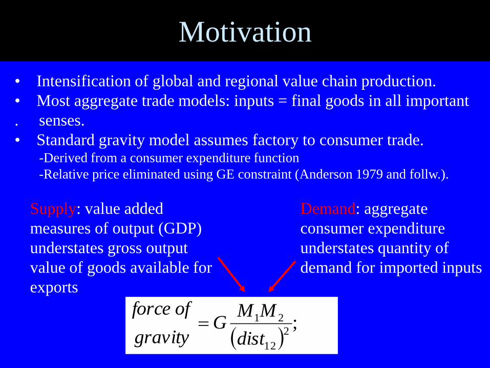
Supply: value added
measures of output (GDP)
understates gross output
value of goods available for
exports
Demand: aggregate
consumer expenditure
understates quantity of
demand for imported inputs
• Intensification of global and regional value chain production.
• Most aggregate trade models: inputs = final goods in all important
. senses.
• Standard gravity model assumes factory to consumer trade. -Derived from a consumer expenditure function
-Relative price eliminated using GE constraint (Anderson 1979 and follw.).
Motivation
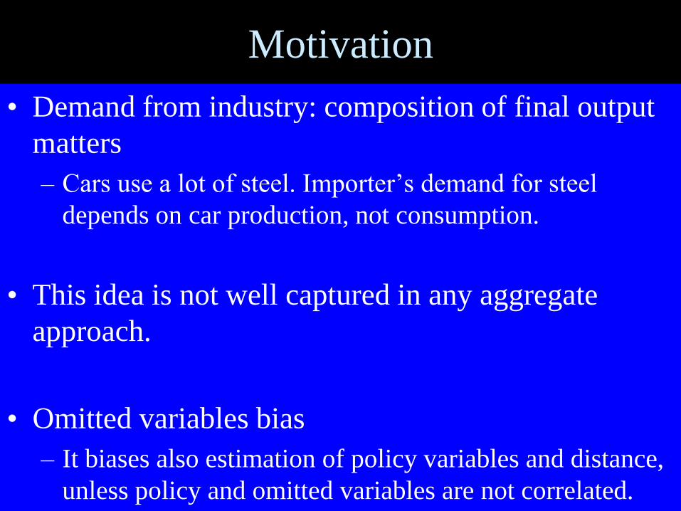
• Demand from industry: composition of final output
matters
– Cars use a lot of steel. Importer‟s demand for steel
depends on car production, not consumption.
• This idea is not well captured in any aggregate
approach.
• Omitted variables bias
– It biases also estimation of policy variables and distance,
unless policy and omitted variables are not correlated.
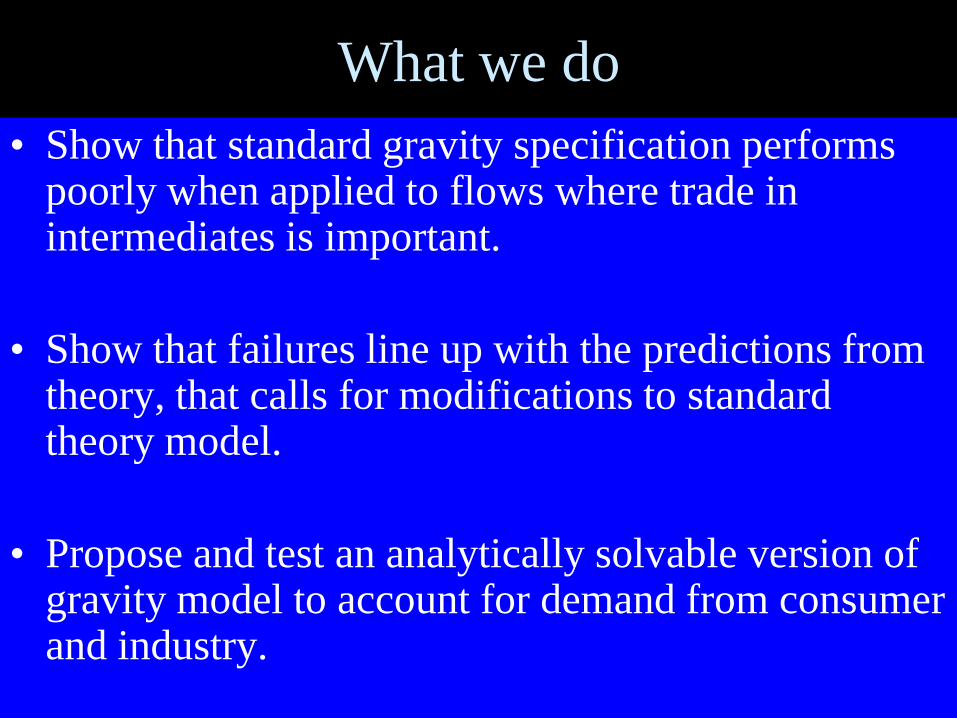
What we do
• Show that standard gravity specification performs poorly when applied to flows where trade in intermediates is important.
• Show that failures line up with the predictions from theory, that calls for modifications to standard theory model.
• Propose and test an analytically solvable version of gravity model to account for demand from consumer and industry.
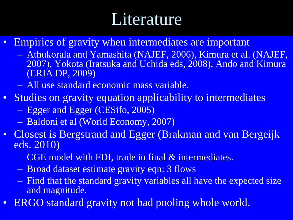
Literature
• Empirics of gravity when intermediates are important– Athukorala and Yamashita (NAJEF, 2006), Kimura et al. (NAJEF,
2007), Yokota (Iratsuka and Uchida eds, 2008), Ando and Kimura (ERIA DP, 2009)
– All use standard economic mass variable.
• Studies on gravity equation applicability to intermediates– Egger and Egger (CESifo, 2005)
– Baldoni et al (World Economy, 2007)
• Closest is Bergstrand and Egger (Brakman and van Bergeijkeds. 2010)– CGE model with FDI, trade in final & intermediates.
– Broad dataset estimate gravity eqn: 3 flows
– Find that the standard gravity variables all have the expected size and magnitude.
• ERGO standard gravity not bad pooling whole world.

Old gravity theory: factory to consumer
• Tinbergen (1962), Pöyhönen (1963).
• Anderson (1979): theoretical explanation based on a CES demand function with Armington product differentiation.
• Refinements show that gravity model is compatible with different theories– Helpman Krugman (1985): Mon. Comp. setting.
– Deardoff (1998): HO setting.
– Eaton and Kortum (2001): Ricardian setting.
– Chaney (2008), Helpman Meliz Rubistein (2008): Application to firm heterogeneity.
;
2
12
21
dist
MMG
gravity
offorce
Gravity: demand equation with a twist
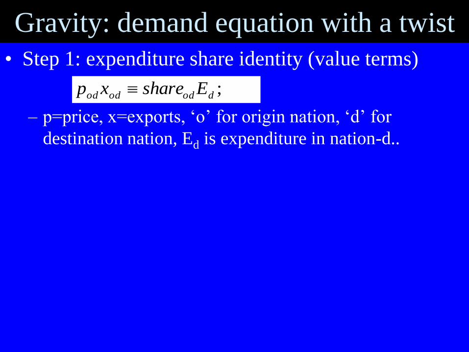
• Step 1: expenditure share identity (value terms)
– p=price, x=exports, „o‟ for origin nation, „d‟ for
destination nation, Ed is expenditure in nation-d..
;dododod Esharexp

Gravity: demand equation with a twist
• Step 1: expenditure share identity (value terms)
• Step 2 (link shares to relative prices, assuming
Dixit-Stiglitz MC):
;dododod Esharexp
1,,)1/(1
1
1
1
R
k kdkd
d
od
od pnPwhereP
pshare
Number of
varieties produced
in nation-k
CES price index of
all varieties
consumed.
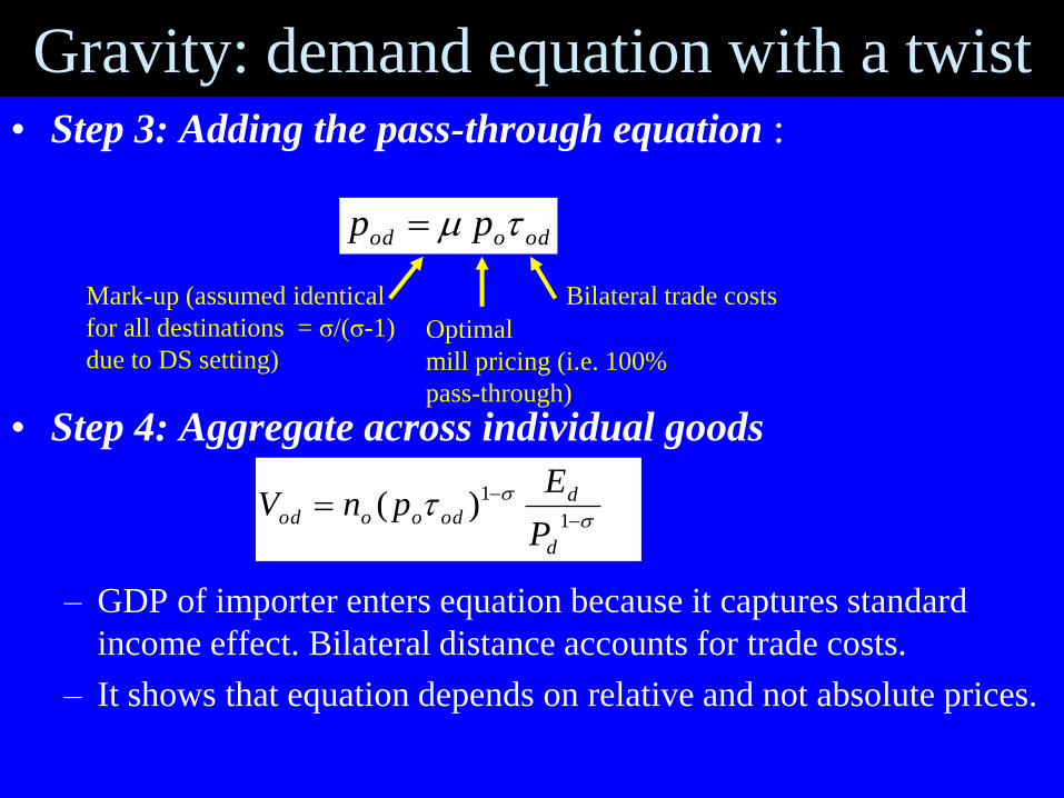
Gravity: demand equation with a twist• Step 3: Adding the pass-through equation :
• Step 4: Aggregate across individual goods
– GDP of importer enters equation because it captures standard
income effect. Bilateral distance accounts for trade costs.
– It shows that equation depends on relative and not absolute prices.
Bilateral trade costsMark-up (assumed identical
for all destinations = σ/(σ-1)
due to DS setting)
odood pp
1
1)(d
dodoood
P
EpnV
Optimal
mill pricing (i.e. 100%
pass-through)
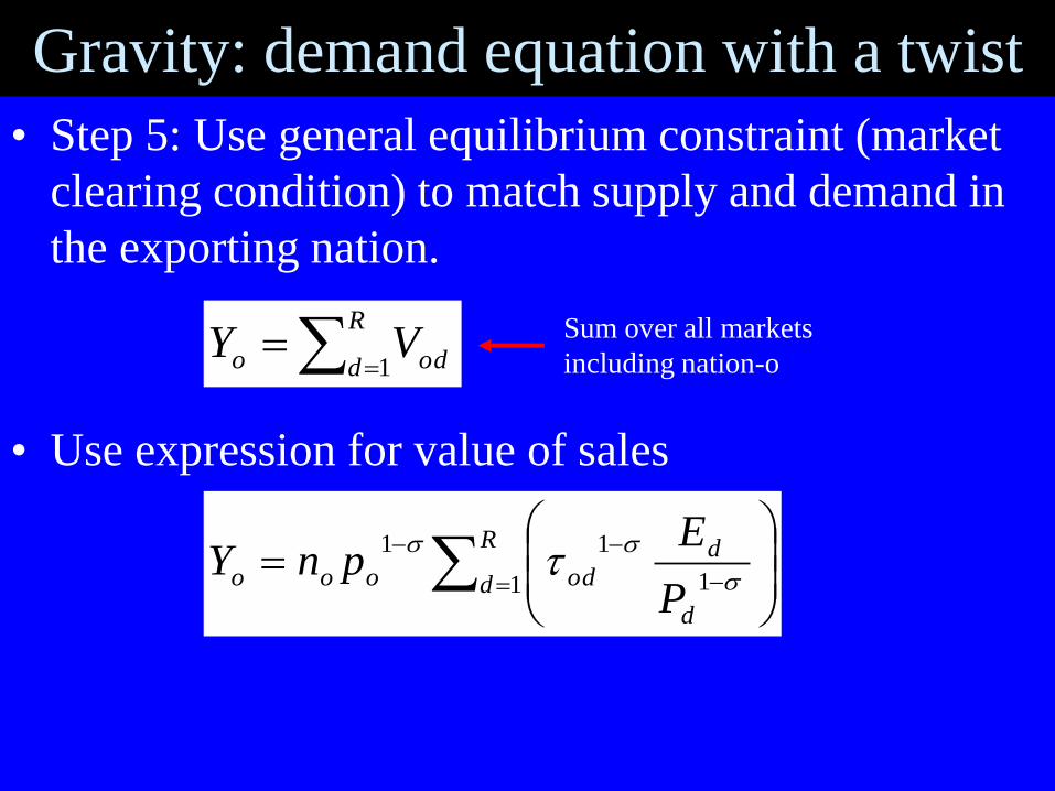
Gravity: demand equation with a twist
• Step 5: Use general equilibrium constraint (market
clearing condition) to match supply and demand in
the exporting nation.
• Use expression for value of sales
Sum over all markets
including nation-o
R
d odo VY1
R
d
d
d
odoooP
EpnY
1 1
11

Gravity: demand equation with a twist
• Solving for the price p that clears the market:
• Plugging it in:
Average of all importers‟ market
demand. Something like a market
potential index for nation-o/
market openness/remoteness.
R
i
i
ioio
o
ooo
P
Ewhere
Ypn
1 1
11)(,
)(1
1
do
doodod
P
EYV
Gravitational
unconstant, i.e.
AvW “multilateral
resistance term”

Our extension of the gravity equation
• Use model where intermediates trade explicitly
addressed:
• Krugman and Venables (EER 1996) vertical
linkages model
– Two goods economy: Walrasian Agr sector and Mon. Comp. Mnf
– Agr produced with L
– Mnf produced with L and CES composite of all varieties (double
use for all varieties)
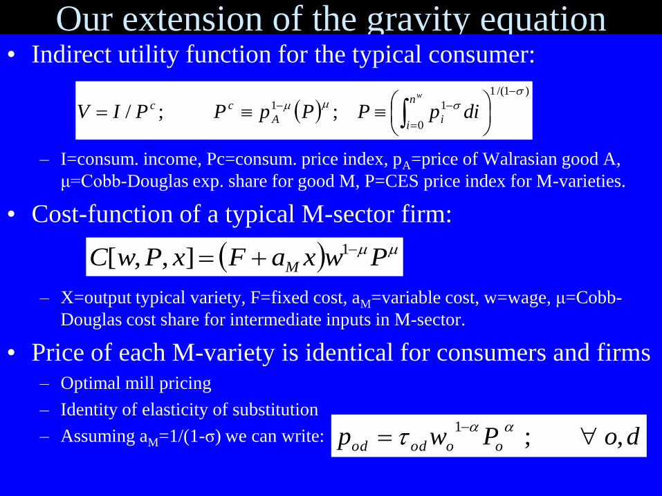
Our extension of the gravity equation• Indirect utility function for the typical consumer:
– I=consum. income, Pc=consum. price index, pA=price of Walrasian good A,
μ=Cobb-Douglas exp. share for good M, P=CES price index for M-varieties.
• Cost-function of a typical M-sector firm:
– X=output typical variety, F=fixed cost, aM=variable cost, w=wage, μ=Cobb-
Douglas cost share for intermediate inputs in M-sector.
• Price of each M-variety is identical for consumers and firms– Optimal mill pricing
– Identity of elasticity of substitution
– Assuming aM=1/(1-σ) we can write:
)1/(1
0
11 ;;/
wn
iiA
cc dipPPpPPIV
PwxaFxPwC M
1],,[
doPwp ooodod ,;1

Direct & Derived Demand
• Hence we obtain a demand function isomorphic to standard
specification, but...
• …now „demand shifter‟ includes Cost & Income
ddddd
d
odod
dood CnIEEP
npV
;
1
1
1
ddddd
d
odod
dood CnIEEP
npV
;
1
1
1
Id=consumer income, Cd=total cost of a typical M-variety.
Direct & Derived Demand
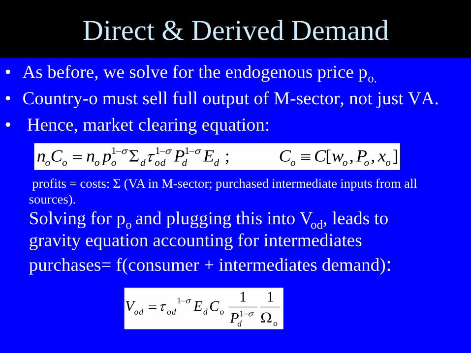
• As before, we solve for the endogenous price po.
• Country-o must sell full output of M-sector, not just VA.
• Hence, market clearing equation:
od
odododP
CEV
111
1
wn
ioii
M
oood
d
odod
ddoo diqpLwCEP
npC01
1
1;
profits = costs: Σ (VA in M-sector; purchased intermediate inputs from all
sources).
Solving for po and plugging this into Vod, leads to
gravity equation accounting for intermediates
purchases= f(consumer + intermediates demand):
],,[;111
ooooddoddoooo xPwCCEPpnCn

BREAKDOWN OF THE STANDARD GRAVITY
MODEL: TESTABLE HYPOTHESES
• Estimated GDP coefficient lower for nations where parts trade is important, and falling as importance of parts trade rises.
– Unless consumer and producer demand move in synch, as in steady state.
• As vertical specialisation trade has become more important over time, the GDP point estimates should be lower for more recent years.
• A more stable relationship should have both consumer and industry in mass variables.

Base specification and data
odt
dt
dt
ot
otodt
P
EYGm ln*ln)ln( 21
•Yot= nation-o output
•Ωot= Market potential:
•constructed as in Baier and Bergstrand (2001)
• σ=4 as Obstfeld and Rogoff (2001) and Carrere (2006).
•Eot= nation-d expenditure
•Pot= nation d export price deflator
Data are from UN-COMTRADE, WB WDI and CEPII.
1
11)(*
d oddtot DistGDP
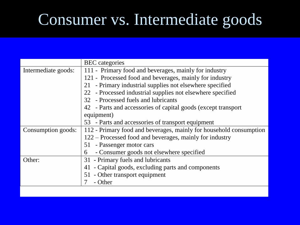
Consumer vs. Intermediate goods
BEC categories
Intermediate goods: 111 - Primary food and beverages, mainly for industry
121 - Processed food and beverages, mainly for industry
21 - Primary industrial supplies not elsewhere specified
22 - Processed industrial supplies not elsewhere specified
32 - Processed fuels and lubricants
42 - Parts and accessories of capital goods (except transport
equipment)
53 - Parts and accessories of transport equipment
Consumption goods: 112 - Primary food and beverages, mainly for household consumption
122 – Processed food and beverages, mainly for industry
51 - Passenger motor cars
6 - Consumer goods not elsewhere specified
Other: 31 - Primary fuels and lubricants
41 - Capital goods, excluding parts and components
51 - Other transport equipment
7 - Other
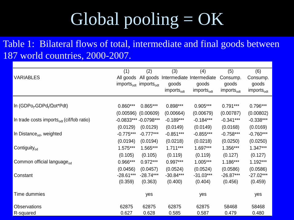
Global pooling = OK
(1) (2) (3) (4) (5) (6)
VARIABLES All goods
importsodt
All goods
importsodt
Intermediate
goods
importsodt
Intermediate
goods
importsodt
Consump.
goods
importsodt
Consump.
goods
importsodt
ln (GDPot*GDPdt/Ωot*Pdt) 0.860*** 0.865*** 0.898*** 0.905*** 0.791*** 0.796***
(0.00596) (0.00609) (0.00664) (0.00679) (0.00787) (0.00802)
ln trade costs importsodt (cif/fob ratio) -0.0833*** -0.0798*** -0.189*** -0.184*** -0.341*** -0.338***
(0.0129) (0.0129) (0.0149) (0.0149) (0.0168) (0.0169)
ln Distanceod, weighted -0.775*** -0.777*** -0.851*** -0.855*** -0.758*** -0.760***
(0.0194) (0.0194) (0.0218) (0.0218) (0.0250) (0.0250)
Contiguityod 1.575*** 1.565*** 1.711*** 1.697*** 1.356*** 1.347***
(0.105) (0.105) (0.119) (0.119) (0.127) (0.127)
Common official languageod 0.966*** 0.972*** 0.997*** 1.005*** 1.186*** 1.192***
(0.0456) (0.0457) (0.0524) (0.0524) (0.0586) (0.0586)
Constant -28.61*** -28.74*** -30.84*** -31.03*** -26.87*** -27.02***
(0.359) (0.363) (0.400) (0.404) (0.456) (0.459)
Time dummies yes yes yes
Observations 62875 62875 62875 62875 58468 58468
R-squared 0.627 0.628 0.585 0.587 0.479 0.480
Table 1: Bilateral flows of total, intermediate and final goods between
187 world countries, 2000-2007.
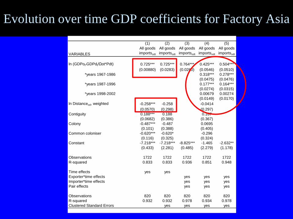
Evolution over time GDP coefficients for Factory Asia
(1) (2) (3) (4) (5)
VARIABLES
All goods
importsodt
All goods
importsodt
All goods
importsodt
All goods
importsodt
All goods
importsodt
ln (GDPot*GDPdt/Ωot*Pdt) 0.725*** 0.725*** 0.764*** 0.425*** 0.504***
(0.00880) (0.0283) (0.0260) (0.0546) (0.0510)
*years 1967-1986 0.318*** 0.278***
(0.0475) (0.0476)
*years 1987-1996 0.177*** 0.164***
(0.0274) (0.0315)
*years 1998-2002 0.00679 0.00274
(0.0149) (0.0170)
ln Distanceod, weighted -0.258*** -0.258 -0.0414
(0.0570) (0.298) (0.297)
Contiguity 0.188*** 0.188 0.167
(0.0682) (0.386) (0.367)
Colony -0.487*** -0.487 0.0695
(0.101) (0.388) (0.405)
Common coloniser -0.620*** -0.620* -0.296
(0.116) (0.325) (0.324)
Constant -7.218*** -7.218*** -8.825*** -1.465 -2.632**
(0.433) (2.281) (0.485) (2.279) (1.178)
Observations 1722 1722 1722 1722 1722
R-squared 0.833 0.833 0.936 0.851 0.948
Time effects yes yes
Exporter*time effects yes yes yes
Importer*time effects yes yes yes
Pair effects yes yes yes
Observations 820 820 820 820 820
R-squared 0.932 0.932 0.978 0.934 0.978
Clustered Standard Errors yes yes yes yes
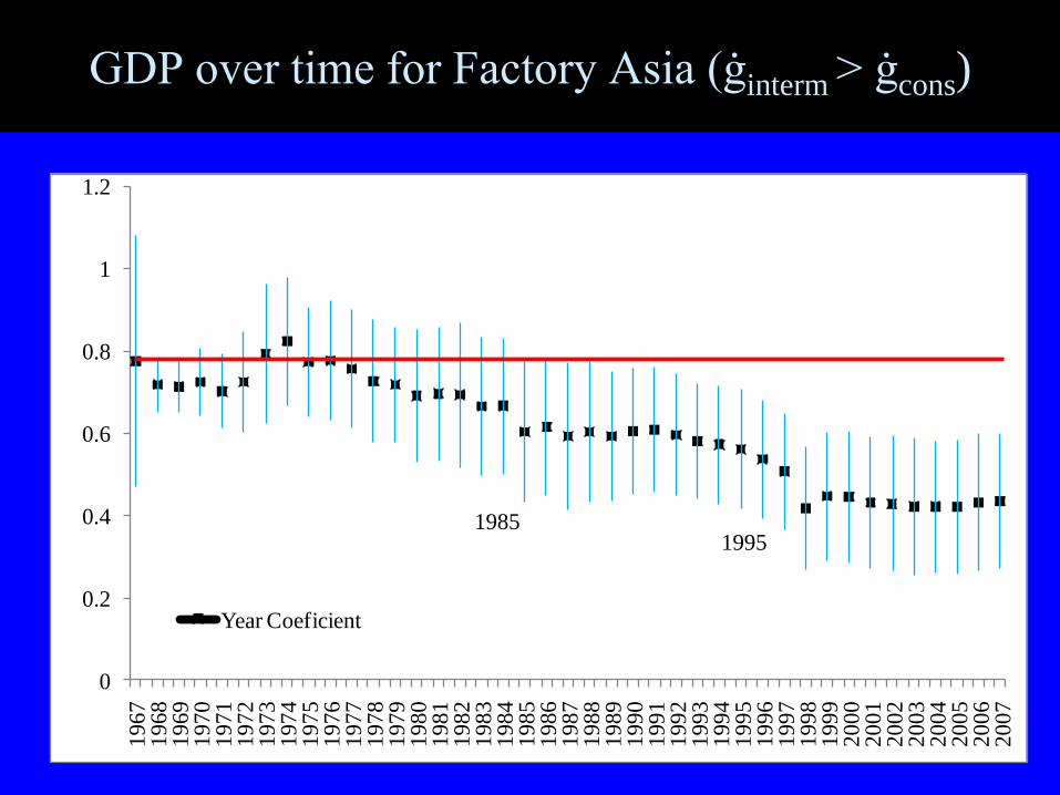
GDP over time for Factory Asia (ġinterm > ġcons)
19851995
0
0.2
0.4
0.6
0.8
1
1.2
19
67
19
68
19
69
19
70
19
71
19
72
19
73
19
74
19
75
19
76
19
77
19
78
19
79
19
80
19
81
19
82
19
83
19
84
19
85
19
86
19
87
19
88
19
89
19
90
19
91
19
92
19
93
19
94
19
95
19
96
19
97
19
98
19
99
20
00
20
01
20
02
20
03
20
04
20
05
20
06
20
07
Year Coeficient
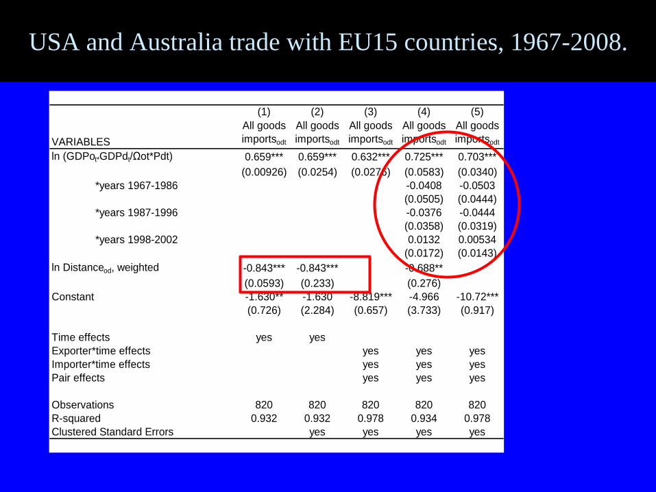
USA and Australia trade with EU15 countries, 1967-2008.
(1) (2) (3) (4) (5)
VARIABLES
All goods
importsodt
All goods
importsodt
All goods
importsodt
All goods
importsodt
All goods
importsodt
ln (GDPot*GDPdt/Ωot*Pdt) 0.659*** 0.659*** 0.632*** 0.725*** 0.703***
(0.00926) (0.0254) (0.0276) (0.0583) (0.0340)
*years 1967-1986 -0.0408 -0.0503
(0.0505) (0.0444)
*years 1987-1996 -0.0376 -0.0444
(0.0358) (0.0319)
*years 1998-2002 0.0132 0.00534
(0.0172) (0.0143)
ln Distanceod, weighted -0.843*** -0.843*** -0.688**
(0.0593) (0.233) (0.276)
Constant -1.630** -1.630 -8.819*** -4.966 -10.72***
(0.726) (2.284) (0.657) (3.733) (0.917)
Time effects yes yes
Exporter*time effects yes yes yes
Importer*time effects yes yes yes
Pair effects yes yes yes
Observations 820 820 820 820 820
R-squared 0.932 0.932 0.978 0.934 0.978
Clustered Standard Errors yes yes yes yes

Summing up
• On data widely recognised as being increasingly
dominated by parts and components we find:
– structural instability in the mass variable
– unusually low coefficients for distance
• On data where trade relationships are stable we find:
– stable mass variables
– coefficients within range
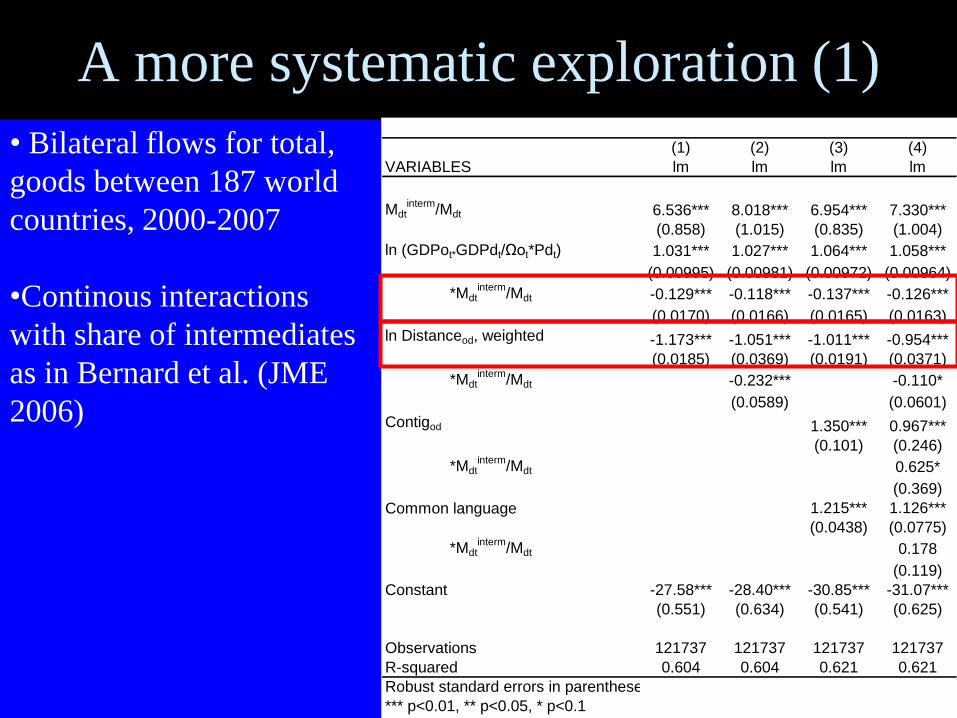
A more systematic exploration (1)
• Bilateral flows for total,
goods between 187 world
countries, 2000-2007
•Continous interactions
with share of intermediates
as in Bernard et al. (JME
2006)
(1) (2) (3) (4)
VARIABLES lm lm lm lm
Mdtinterm
/Mdt 6.536*** 8.018*** 6.954*** 7.330***
(0.858) (1.015) (0.835) (1.004)
ln (GDPot*GDPdt/Ωot*Pdt) 1.031*** 1.027*** 1.064*** 1.058***
(0.00995) (0.00981) (0.00972) (0.00964)
*Mdtinterm
/Mdt -0.129*** -0.118*** -0.137*** -0.126***
(0.0170) (0.0166) (0.0165) (0.0163)
ln Distanceod, weighted -1.173*** -1.051*** -1.011*** -0.954***
(0.0185) (0.0369) (0.0191) (0.0371)
*Mdtinterm
/Mdt -0.232*** -0.110*
(0.0589) (0.0601)
Contigod 1.350*** 0.967***
(0.101) (0.246)
*Mdtinterm
/Mdt 0.625*
(0.369)
Common language 1.215*** 1.126***
(0.0438) (0.0775)
*Mdtinterm
/Mdt 0.178
(0.119)
Constant -27.58*** -28.40*** -30.85*** -31.07***
(0.551) (0.634) (0.541) (0.625)
Observations 121737 121737 121737 121737
R-squared 0.604 0.604 0.621 0.621
Robust standard errors in parentheses
*** p<0.01, ** p<0.05, * p<0.1
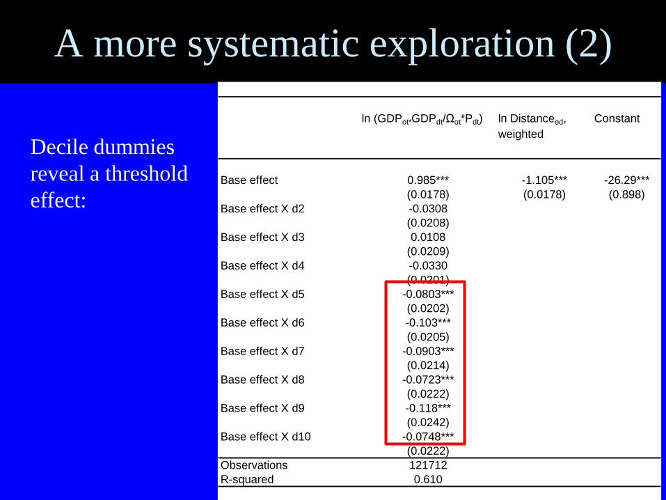
A more systematic exploration (2)
ln (GDPot*GDPdt/Ωot*Pdt) ln Distanceod,
weighted
Constant
Base effect 0.985*** -1.105*** -26.29***
(0.0178) (0.0178) (0.898)
Base effect X d2 -0.0308
(0.0208)
Base effect X d3 0.0108
(0.0209)
Base effect X d4 -0.0330
(0.0201)
Base effect X d5 -0.0803***
(0.0202)
Base effect X d6 -0.103***
(0.0205)
Base effect X d7 -0.0903***
(0.0214)
Base effect X d8 -0.0723***
(0.0222)
Base effect X d9 -0.118***
(0.0242)
Base effect X d10 -0.0748***
(0.0222)
Observations 121712
R-squared 0.610
Decile dummies
reveal a threshold
effect:

A more systematic exploration (2)1
ln *ot dt
ot dt
Y E
P
0.8
0.9
0.9
1.0
1.0
1.1
0% 10% 20% 30% 40% 50% 60% 70% 80% 90%
siz
e c
oe
ffic
ien
t
share of intermediates in total imports
Decile dummies reveal a threshold effect:
Search for mass proxies when
intermediates trade mattersTheory suggests that:
• To construct supply shifter one needs data on total
output.
• To construct demand shifter one needs data on total
costs.
• Data on gross output or gross sales acceptable (with
some caveats) but not widely available.
• Hence we searched for a pragmatic repair.
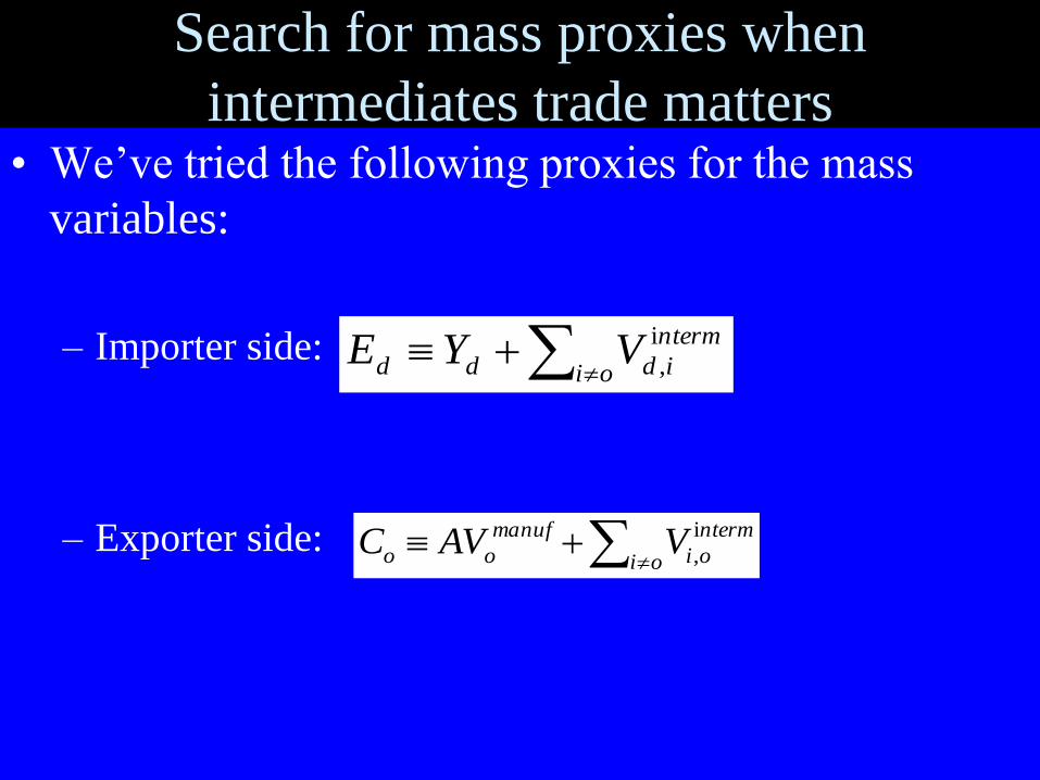
Search for mass proxies when
intermediates trade matters• We‟ve tried the following proxies for the mass
variables:
– Importer side:
– Exporter side:
oi
nterm
iddd VYE i
,
oi
nterm
oi
manuf
oo VAVC i
,
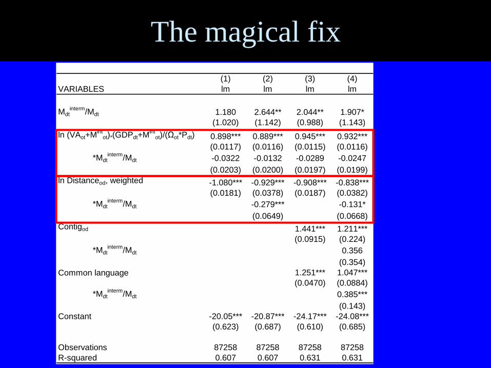
The magical fix
(1) (2) (3) (4)
VARIABLES lm lm lm lm
Mdtinterm
/Mdt 1.180 2.644** 2.044** 1.907*
(1.020) (1.142) (0.988) (1.143)
ln (VAot+Mint
ot)*(GDPdt+Mint
ot)/(Ωot*Pdt) 0.898*** 0.889*** 0.945*** 0.932***
(0.0117) (0.0116) (0.0115) (0.0116)
*Mdtinterm
/Mdt -0.0322 -0.0132 -0.0289 -0.0247
(0.0203) (0.0200) (0.0197) (0.0199)
ln Distanceod, weighted -1.080*** -0.929*** -0.908*** -0.838***
(0.0181) (0.0378) (0.0187) (0.0382)
*Mdtinterm
/Mdt -0.279*** -0.131*
(0.0649) (0.0668)
Contigod 1.441*** 1.211***
(0.0915) (0.224)
*Mdtinterm
/Mdt 0.356
(0.354)
Common language 1.251*** 1.047***
(0.0470) (0.0884)
*Mdtinterm
/Mdt 0.385***
(0.143)
Constant -20.05*** -20.87*** -24.17*** -24.08***
(0.623) (0.687) (0.610) (0.685)
Observations 87258 87258 87258 87258
R-squared 0.607 0.607 0.631 0.631
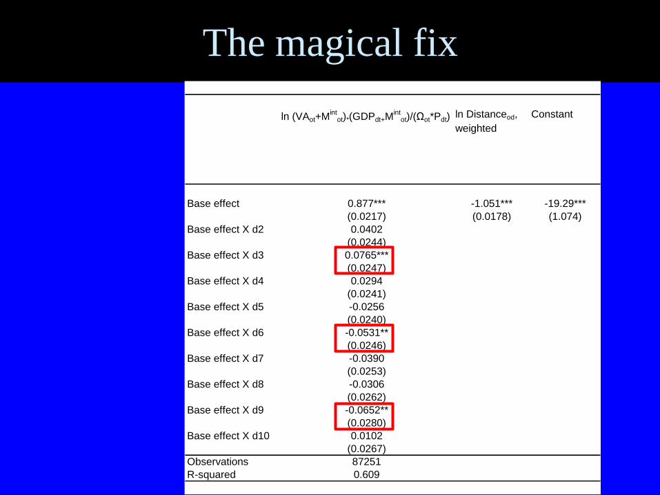
The magical fix
ln (VAot+Mint
ot)*(GDPdt+Mint
ot)/(Ωot*Pdt) ln Distanceod,
weighted
Constant
Base effect 0.877*** -1.051*** -19.29***
(0.0217) (0.0178) (1.074)
Base effect X d2 0.0402
(0.0244)
Base effect X d3 0.0765***
(0.0247)
Base effect X d4 0.0294
(0.0241)
Base effect X d5 -0.0256
(0.0240)
Base effect X d6 -0.0531**
(0.0246)
Base effect X d7 -0.0390
(0.0253)
Base effect X d8 -0.0306
(0.0262)
Base effect X d9 -0.0652**
(0.0280)
Base effect X d10 0.0102
(0.0267)
Observations 87251
R-squared 0.609
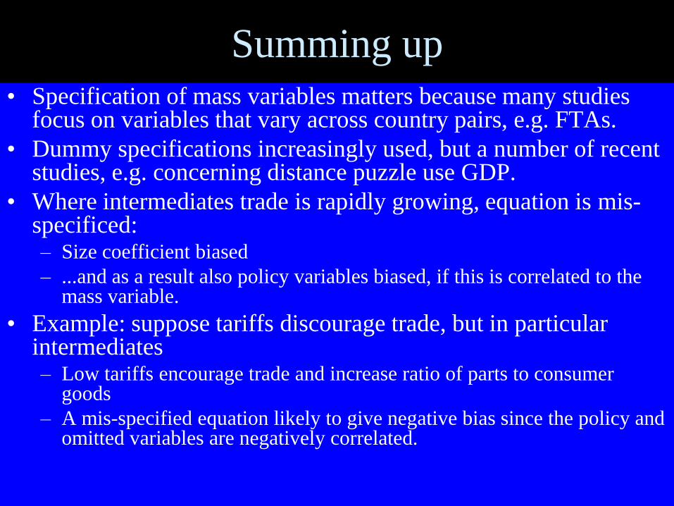
Summing up• Specification of mass variables matters because many studies
focus on variables that vary across country pairs, e.g. FTAs.
• Dummy specifications increasingly used, but a number of recent studies, e.g. concerning distance puzzle use GDP.
• Where intermediates trade is rapidly growing, equation is mis-specificed: – Size coefficient biased
– ...and as a result also policy variables biased, if this is correlated to the mass variable.
• Example: suppose tariffs discourage trade, but in particular intermediates– Low tariffs encourage trade and increase ratio of parts to consumer
goods
– A mis-specified equation likely to give negative bias since the policy and omitted variables are negatively correlated.
What next?
• Tested hypotheses confirm insights from the theory.
• Refine suggestions of ways in which the theoretical model
can be implemented empirically.
• Focus on distance.
– Distance seems to matter more for parts & components than for
consumption goods.
• Different elasticity of demand.
• Coordination of production issues.
• But no easy fix
– Composition of supply/demand may respond to differential trade
costs.
• I am close to a car producer; I endogenously choose to produce steel inputs
used in cars.
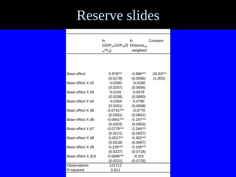
Reserve slides
ln
(GDPot*GDPdt/Ω
ot*Pdt)
ln
Distanceod
, weighted
Constant
Base effect 0.978*** -0.996*** -26.93***
(0.0178) (0.0596) (1.003)
Base effect X d2 -0.0300 -0.0189
(0.0207) (0.0695)
Base effect X d3 0.0109 0.0578
(0.0208) (0.0680)
Base effect X d4 -0.0304 0.0780
(0.0201) (0.0658)
Base effect X d5 -0.0741*** -0.0779
(0.0201) (0.0651)
Base effect X d6 -0.0941*** -0.197***
(0.0203) (0.0653)
Base effect X d7 -0.0778*** -0.246***
(0.0211) (0.0657)
Base effect X d8 -0.0517** -0.302***
(0.0218) (0.0697)
Base effect X d9 -0.105*** -0.190***
(0.0237) (0.0718)
Base effect X d10 -0.0689*** -0.101
(0.0221) (0.0725)
Observations 121712
R-squared 0.611
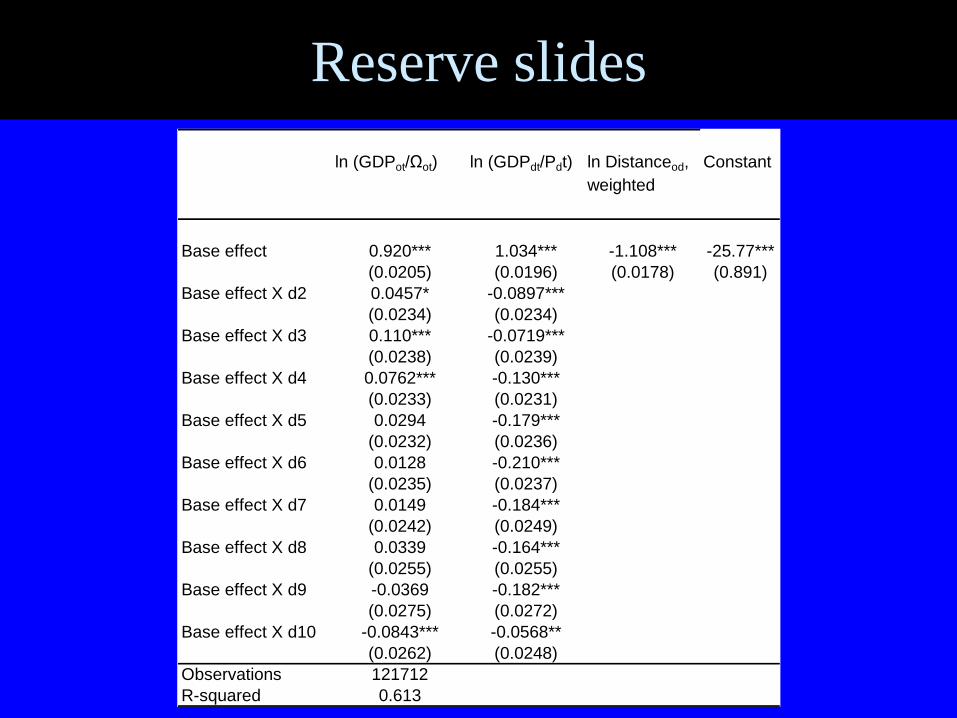
Reserve slides
ln (GDPot/Ωot) ln (GDPdt/Pdt) ln Distanceod,
weighted
Constant
Base effect 0.920*** 1.034*** -1.108*** -25.77***
(0.0205) (0.0196) (0.0178) (0.891)
Base effect X d2 0.0457* -0.0897***
(0.0234) (0.0234)
Base effect X d3 0.110*** -0.0719***
(0.0238) (0.0239)
Base effect X d4 0.0762*** -0.130***
(0.0233) (0.0231)
Base effect X d5 0.0294 -0.179***
(0.0232) (0.0236)
Base effect X d6 0.0128 -0.210***
(0.0235) (0.0237)
Base effect X d7 0.0149 -0.184***
(0.0242) (0.0249)
Base effect X d8 0.0339 -0.164***
(0.0255) (0.0255)
Base effect X d9 -0.0369 -0.182***
(0.0275) (0.0272)
Base effect X d10 -0.0843*** -0.0568**
(0.0262) (0.0248)
Observations 121712
R-squared 0.613