Jumal Kejurutcrun 1 (1989) 9$-108

Gravity Drainage of a Stratified Profile

S. Awadalla

ABSTRACT

The Green and Ampt approach was developed for the falling water table case following an initial sudden drop in the position of the water tdble. The dnalysis pusent. an approximtJte solution' for one-dimensional flow in saturated 'porous media. The for­mulation is based on calculating the position of draininj front .with time aM the cumulative outflow time relationship"' for stratijWd profile. The Green and Ampt results are checlted by using tUta obtained from a well-proven computer-based nu­mericd/ ' solution for unsaturated flow equdtion involving dn

implicit finite difference approach.

ABSTRAK

Pendekatan Green dan Ampt telah dikembanglllln , untuk kes kejatuhan tiras air tdnah melalui kejatuhan awal tiba-tiba di dalam kedudukan aras air tanah. Analisa ini mempersembahkan penyele­saian hampiran untuk aliran dimensi di dalam ruang (media) telap tepu. Formulasi ini bero/lSarkan pengiraan kedudukan mulla aliran lie luar-masa untuk rautan distratum. Basil Green dan Ampt ada­lah diperillsa dengan menggunakdn data )lang diperoleki daTi penyelesaian berangka berasaskan komputer untuk persdmaan aliran tal tepu yang melibatkan pendekatan perbez/ldn terhingga yang tersirat.

INTRODUCTION

Green and Ampt (1911) devdoped a sharp front analysis to describe vertical water movement during infdtration. For such a regime. the resulting infdtration equation and its application to laboratory and field, conditions have received considerable attention. The sharp front concept can also be applied to drainage conditions, and analysis of this , type was presented by Childs (1969) to describe the gravity drainage to a stationary water table of an initially saturated porous material. Earlier. Youngs (1960). had used a capillary bundle model to derive a drainage equation in simple algebraic form. The ability of the Green and Ampt approach to describe satisfactorily drainage processes to a sta­tionary water table relates among other factors to the shape of the soil water characteristic for the porous material in question. In general. for coarse porous material exhibiting a 'steep' soil

96

water characteristic the equation represents the outflow time relationship satisfactorily during the early stage of drainage. However, as the increasing 'spread' of the drainage front becomes significant at longer periods of time the analysis loses its appli. cability as would be expected. Watson and Whisler (1976) indicate that for gravity drainage to a stationary water table the Young' equation gives results more closely aligned to computer based n!,merical results than the 'complete' Green and Empty equation. The stationary water table studies assume an initial instantaneous drop in position of the water table.

Young and Aggelides (1976) presented an equation based on the Green and Ampt assumptions for gravity drainage under a falling water table yet without any initial step change of water table position. Their analysis typified a land drainage environment with the water table initially positioned at the soil surface and then moving gradually downwards at soine prescribed rate.

The present study has as its aim a detailed evaluation of the adequacy or otherwise of the Green and Ampt approach for the falling water table problem for stratified medium sand using a well·proven. computer based numerical analysis of the unsaturated flow equation for comparative purposes. In the following section the general Green and Ampt equations are developed for both zero and nonzero applied surface flux. These equations are used to give results for a range of falling water table conditions. These results are then compared with the numerica) simulations and conclusions are drawn legarding the accuracy of the approximate equations in modeling the falling water table regime.

THE ONE DIMENSIONAL DIFFERENTIAL FLOW EQUATION

The general partial different equation for flow in rigid unsaturated porous media can be derived by combining Darcy's law with the equation of continuity. The equation for vertical flow as,

C(h) ilh = ~ (K(h) ilh) + ilK(h) at ilz 'ilz ilz

where

C(h) specific capacity cm

h pressure head cm- 1

z is cartesian co·ordinates cm

K hydraulic conductivity cm/min

NUMERICAL APPROACH

(1)

The partial derivatives of equation (1) are approxintated by the finite different equation given below. To find the finite different expression at node i, the pressure head and soil characteristic

at the node above, (node i-I) and the node below i (node i + 1) are required_ The distance between each two nodes can be defined by z = L/N where N is the· number of nodes_

h (i + I, j + 1/2) = 1/2 [h (i + I,j) + h (i + I, j + 1)](2)

h (i, j + 1/2) = 1/2 [h (i,j) + (i, j + I)) (3)

h (i - l,J + 1/2) = 1/2 [h (i - l,j) + (i -l,j + I)) (4)

Therefore the right hand side of the equation (1) can be evaluated from the following expressions_

ah (i+l/2, j+l/2) = (1/2~z) [h(i+l,j+l) az

+ h(i+l,j)-h(i,j+l)

h(i,m (5)

ah (i - 1/2,j + 1/2) = "(1/2 ~ z) [h (i,j + 1) Oz

+ h(i,j) - h(i - j,j + 1)

- h(i - 1, j) ]

~ [K(h) ~h (i, j + 1/2) = [K(i+ 1/2, j + 1/2) Oz oZ

oh (i + 1/2, j + 1/2) oz

- K(i - 1/2, j - 1/2)

~~ (i - 1/2, j - 1/2)) I&.

:z [K(h)) (i, j + 1/2) = K(i - 1/2, j + 1/2)]

(6)

- K(i - 1/2, j + 1/2)] &. (8)

C(H) oh (i, j + 1/2) = C(i, j + 1/2)[h(i, j + 1) at

- h(i, j)l /~t

substituting equations (5) to (9) into equatiolU (1)

C(i, j + 1/2) [h(i, j + 1) - h(i, j)] I~t =

(9)

97

K(i - 1/2, j + 1/2) [h(i + I, j) + h(i + 1) - h(i, j) - h(i "j + 1)1/2 (~)2

98 1 ~ K(i -1/2,j +1/2) [h(i,j) + h (i,j + 1) - h(i -1,j+ 1)

_ h(i - 1,j)] /2 (&)2 + [K(i + 1/2,j + 1/2)

- K(i - 1/2)] / (&) (10)

Let

K(i + 1/2,j · ... l/2) = [K(i + 1,j) + K(i + l.j + 1)

+ K(i,j + 1) + K(i,j) 1/4 (11)

K(i -1/2, j + 1/2) = [K(i, j + 1) + K(i,j)

+ K(i-1,j+1)+K(i - 1,j)J/4 (12)

Equation (141) can be rearranged in general form as

Aih (i-l,j+1)+Bjh(i,j+1)+Ci h (I+1,j+1) = Di (13Y

Where all the tenns at the previous time (j) are on the right hand side, Di. The coefficient can then be written as follows

• Ai = -K(i - 1/2,j + 1/2)/2 (&)2

Cj = -K(i + Ito!, j + 1/2)/2 (&)2

Bj = C(i,j + 1/2) 6t - Ai - Cj

Di + -Aih(i - 1,j) + [C(i,j + 1/2) / t + Ai + Cj] h(i,j)

-Cjh(i + 1,j) + 2 67. (Ai - Cj)

(14)

(15)

(16)

(17)

Equation (13) constitutes a set of n-1 algebraic equations in n + 1 knowns. The -solution of _ the question requires the appli· cation of a top and bottom boundary condition to eliminate the terms in hI and hn + 1 respectively. To remove the nonlinearity in the equation, an iterative process is used in which an initial value of b (i, j + 1) at each point is specified and this is used to determine the coefficients Ai ' Bi ,Cj and Di' The initial condi­tion is used as the first set of h(i, j) values for the purpose of evaluating Ai • Bj • Cj and Di' The resulting set of linear algebraic equations is solved by an algorithm for an improved estimate of h(i, j + 1) values. This improved ~stimate of h(i, j) is in tum used to get new values of Ai , Bj , Cj and Di and a second improved estimate of h(i, j + I) Yalues is obtained. The process is continued until satisfactory convergence occurs.

99

The uppel: boundary condition during gravity drainage is that of zero flux and may be written;

-K(h) [ ~: + 1 1 z = 0 = 0 t > 0 (18)

At the lower boundary the gauge pressure is zero and consequent­ly

h(h, t)z = 0 = 0 t > 0 (19)

The boundary condition described by equation (19) is the pre­sence of the water table_ As long as the lower part remains satu­rated, the flux through this layer is given by:

Where hi (t) = the pressure head at the interface.

If the air entry value of ' the main profile is dermed as hAEV, then the initial condition becomes:

t = 0 z = 0 h = hf (20)

t = 0 z = Lu h = h;o

t = 0 z = -Lh = 0

The pressure head profile in each layer at t = ~ is a straight line and may be written:

-Lu < z < 0 (21 )

By applying Darcy's law and the continuity equation, h is given by

= hf Ku (Zu - L) - (zu - L) (Ku - Ku) zu

Ku (Zu - L) - KL zu (22)

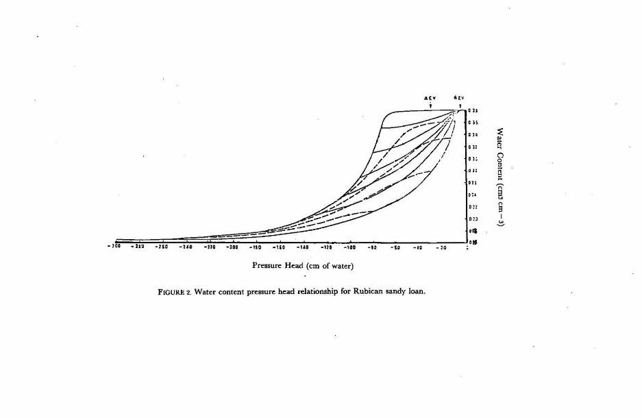
The porous materials used in the numerical analysis were Botany Sand and Rubicon Sandy loam. The water content (9) soil water pressure (h) relationship for these materials are given in Figure 1 and Figure -2. In the case considered, the thickness of the drainage proflie (Lu) was 95 cm. This was supported by a layer

. whose thickness (LL) waS 5 cm. The saturated hydraulic con­. ductivity for Lu was 8 cm/min and LL was ~3 em/min.

100

..._------:::;.-----j°. ""

_6~O---L--~-~.O~~--~-.~O~-L--~-~30~~--~-~20~--L-~-I~

PRESSURE HEAD (em of .water)

FIGURE 1. h (0) relationship for No. 17 sand.

THE GREEN AND AMPT ANALYSIS

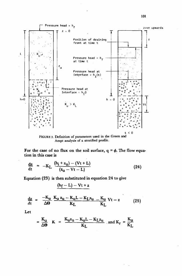
The definition of significant parameters for the stratified case is shown in Figure 3. In particular, z is the thickness of the upper layer and, as Figure 3 indicates I L I < Zu When the draining front reaches the interface the analysis for the lower layer is again of the homogeneous profile form with an appropriate change in the value of 6.9 because of the change in material characteristics across the interface. In this study Ku' > KL , thus giving a coarse over fine sequence. The analysis of such a sequence presents no problem; however, gravity drainage of the reverse sequence (i.e. Ku <KL) with tl)e assumption that air can only enter the profile through the surface presents some physical complexities involving pore air pressure changes at the interface. This phenomenon has been discussed by Watson and Whisler (1977) and Watson (1968). In the case of a stratified profile it is often convenient to know the initial pressure head value at the interface. For the configuration of Figure 3 this pressure head is given by equation 22. However, in this case, time dependent pressure head, hi (t), at the interface is required. This may be written as

hi(t) = Ku(hf + Z - Zu)(Zu - Vt ~ L) - Kdz - Zu)(Zu - Vt - L)

KL(z - Zu) + Ku(Zu - Vt - L)

(23)

L

h=O

r Pressur e

'.

. ,

~f' . t'"

head hf

Zu

Z = 0

Position of draining front at tirwe t

Pressure head hf at tillte t

Pressure head at int~rface = hi(tl

Pressure head at interface = h

iO

r

I

h o

t < 0 FIGURE 3. Definition of parameters used in the Green and

Ampt analysis of a stratified profile.

101

l+\le

1

For the case of no flux on the soil surface, q = tP. The flow equa· tion in this case is .

dz dt

= K (hi+zu)-(Vt+L)

- L (Zu - Vt - L)

Equation (23) is then substituted in equation 24 to give

(hf - L) - Vt + z

dz = -Ku Ku Zu - KuL - KLZu Ku Vt - z dt lI9 KL KL

Let

= Ku K = Kuzu - KuL - KLZu . andKr = lI9 KL

(24)

(25)

Ku

KL

upwards

-J CO -:';2-1' -150 -uo -no -III

.~:--'~--­---::;,,~,;-:::,::::' ----

-110 -1511 -ua -no -\00

Pressure Head (em of water)

...

-u -" -"

FIGURE 2. Water content pressure head relationship for Rubican sandy loan.

::E ~ o

i § S I ~

'Then equation 25 becomes '

dz = - .0 'Vt + z + (.0 'hf - .0 'L) dt Kr Vt - z - K '

The fmal solution of equation (26) is as follows:

In(-j) = lin 2

-A + (a - B) u + bu'

k bk' -A + (a - B) ~ + -J j'

103

(26)

+ a+B In 2-1i

k a - B + 2bu - "'-Ii (a - B) + 2b T + V-Ii

k a-B+2bu+v-li (a-B)+ 2b T -V-I)

(27)

Equation (27) represents the Green and Ampt flow equation for a 'stratified profile under falling water table conditions with q = ",.", em/min. The coefficients from equation (26) may be listed as

A = -n' B = .0', C = n'(hf-L) a =K . r ,b = -1 and c =-K

the other parameters being

j = hf-L-K'

V(1 - Kr) k = Kdhf - L) - K '

l-Kr

-6 = V4n'V+(KV- ')'

= t-jandu =!!. = z-k , t-j

(28)

(29)

(30)

Equation (27) may seem an' awkward equation to use; however, for a given system, all the terms on the right hand side are cons­tant except for u. This results in a minimum of calculation in arriving at the position of draining front z for a fiiven value of t-

104

COMPARISON BETWEEN THE GREEN AND AMPT ANALYSIS AND NUMERICAL RESULTS

The numerical method used in the calculation of drainage of a stratified profIle is compared with the Green and Ampt results. Obviously the initial pressure head distribution is different but this can readily be determined by calculating h using Equation 6. In addition, there must be pressure head continuity across the interface and this condition sometimes requires grid refIning in

Pressure He"d (CIIl)

-100 -90 -80 -70 -60 -~O -40 ..!/!.

100

FIGURE 4, h( .. • .... )profiles for a stratified column with L - 100 em, V = - 2.0 em/min and q. = 0.0 em/min. The numerals on the profUes represent the time minutes from the start of the simulation.

200

·10

·20

·30

·40

·50

·60

·70

·'o ·'0

-100

-110

-120 iii ~

-130 ;!

-140 Q -I~)

-100

-l70

-lBO

-190

-1 -l'00 -2l0

-220

-230

-24<l

-250

-26-

-no -2flO

-29-

-lOO

the vicinity of the interface. The sequence of porous materials is used in the comparative study of thinning in the vicinity of the interface. The sequence of porous materials is used in the com· parative study of this section were No. 17 sand is supported by r8Asand.

The thickness of the top layer for the profile was 95 em. The length of the column· is L = 100 em. The initial 8(z) in each

i' ~ I ~

"-'" 0

105

layer is set to the value corresponding to the initial h(z) values resulting in a water content discontinuity across the interface. The case was considered with V = 2.0 em/min, this being for q = 0.0 em/min. The numerical h(z) profiles are shown in Figure 4 and the e(~) profiles in Figure 5. The cumulative drainage outflow and the thickness of capillary fringe versus time for the

-10

-20

-30

-40

-50

-60

-70

-80

-90 -100

-120

-130

-140

-150 -160

-170

-180

-190

-200

-210

-220

-230

-240

-250

-260 -270

-280

-290

-300

WATER CONTENT (ee/ee)

.0 .0'

100

t

FIGURE 5.0 (z) profiles for a stratified column with L = - 100 em, V = - 2.0 em/min and q = 0.0 em/min. The numerals on the profiles represent the time in minutes form the start of the simulation

106

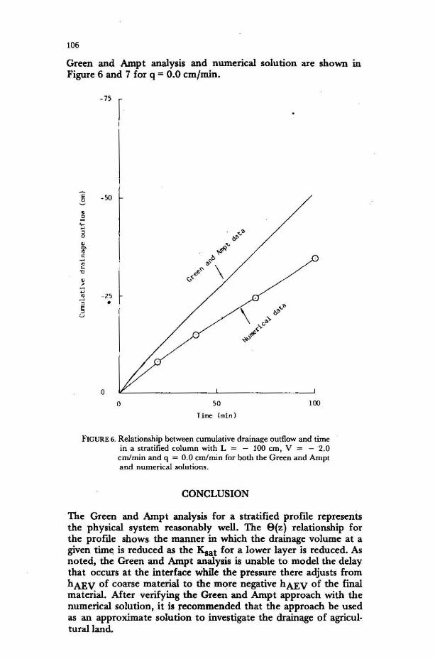
Green and Ampt analysis and numerical solution are shown in Figure 6 and 7 for q = 0.0 cm/min .

• 75

- 2> •

o o SO 100

, i me (min)

FIGURE 6. Relationship between cumulative drainage outflow and time in a stratified column with L = - 100 em , V = - 2.0

emlmin and q = 0 .0 cmlrnin for both the G reen and Ampt and numerical solutions .

CONCLUSION

The Green and Ampt analysis for a stratified prome represents the physical system reasonably well. The 8(z) relationship for the prome shows the manner in which the drainage volume at a given time i. reduced as the Ksat for a lower layer is reduced. As noted, the Green and Ampt analysis is unable to model the delay that occurs at the interface while the pressure there adjusts from h AEV of coarse material to the more negative h AEV of the final material. After verifying the Green and Ampt approach with the numerical solution, it is recommended that the approach be used as an approximate solution to investigate the drainage of agricul. turalland.

e <.>

~

e 0 ~ ~

'" e

.= .. ~

'C

~

0

e .£ ~

~ 0 a.

Time (min)

O~O ________ -.-,,-__ ~~;-________________ ~lO.OO

-100

- 200

-300

G&A N

Draining front reaches the interface at these times

rical data 1 Green

/ -100

and Ampt data

Drai ning front position

Post tion of water tabl

FIGURE 7. Relations between the thickness of the capillary fringe "and time in a stratified column with L = - 100 em, V = 12.0 em/min and q = 0.0 em/min for both the Green and Ampt and numerical solutions.

108

C(h) h z hf L 68

Ksat

NOTATION

specific capacity cm pressure had cm cartesian coordinates cm air entry value cm initial distance of the water table cm difference between saturated water content and residual water content ~aturated hydraulic conductivity

REFERENCES

Childs, E. C. 1969. An Introduction to tM Ph.ysical Basis of Soil Water Phenomena. London: Wiley - Interscience.

Green, W. H. and C. A. Ampt 1911. Studies on Soil Physics I: The flow of air and water through soils. J. Agr. 4: 1-24.

Watson, K. K. 1968. Water content - pressure head relationship. Soil Sci. Soc. Am. Proc. 32, 882-892.

Watson and Whisler. 1976. Comparison of drainage equation for the gravity drainage of stratified profiles. Soil Sci. Soc. Am. J: 631-635.

Watson and Whisler. 1977. Profile desaturation during sediment deposition in a groundwater recharge trench. J. Hydro/, 33; 397-401.

Youngs, E. C. 1960. The drainage ofliquids from porous materials.]. Geophys. Res. 65, 4205-4030.

Youngs, E. G. and S. Agge1ides. 1976. Drainage to a water table analysed the Green-Am.pt approach. J. Hydrol 31: 67-79.

Fakulti Kejuruteraan Universiti Kebangsaan Malaysia 43600 UKM Bangi Selangor D.E., Malaysia.