Great Lakes Water Quality Initiative technical support ... · United States Environmental...

United StatesEnvironmental ProtectionAgency

Office of Water4301

EPA-820-B-95-005March 1995

Great Lakes WaterQuality InitiativeTechnical SupportDocument for theProcedure toDetermineBioaccumulationFactors

DISCLAIMER

This document has been reviewed by the Health and EcologicalCriteria Division, Office of Science and Technology, U.S.Environmental Protection Agency, and approved for publication as asupport document for the Great Lakes Water Quality Initiative. Mention of trade names and commercial products does not constituteendorsement of their use.

ACKNOWLEDGEMENTS

Technical support for preparation of this document was provided tothe Office of Water by Charles E. Stephan, Lawrence Burkhard, andPhil Cook of the Office of Research and Development, EnvironmentalResearch Laboratory, Duluth. MN.

AVAILABILITY NOTICE

This document is available for a fee upon written request ortelephone call to:

National Technical Information Center (NTIS)U.S. Department of Commerce

5285 Port Royal RoadSpringfield, VA 22161

(800) 553-6847(703) 487-4650

NTIS Document Number: PB95187290

or

Education Resources Information Center/Clearinghouse for Science,Mathematics, and Environmental Education (ERIC/CSMEE)

1200 Chambers Road, Room 310Columbus, OH 43212

(800) 276-0462(614) 292-6717

ERIC Number: D049

i

GREAT LAKES WATER QUALITY INITIATIVE TECHNICAL SUPPORT DOCUMENTFOR THE PROCEDURE TO DETERMINE BIOACCUMULATION FACTORS

TABLE OF CONTENTS

Page

I. INTRODUCTION . . . . . . . . . . . . . . . . . . . . . . . . . . . . . . . . . . . . . . . . . . . . . . . . . . . . . . . 1A. Purpose and Scope . . . . . . . . . . . . . . . . . . . . . . . . . . . . . . . . . . . . . . . . . . . . . . . . 1B. Overview of Bioaccumulation and Bioconcentration . . . . . . . . . . . . . . . . . . . . . . 1C. Outline of the Methods for Deriving Baseline BAFs . . . . . . . . . . . . . . . . . . . . . . 2D. GLI BAFs . . . . . . . . . . . . . . . . . . . . . . . . . . . . . . . . . . . . . . . . . . . . . . . . . . . . . . . . . 2E. Definitions . . . . . . . . . . . . . . . . . . . . . . . . . . . . . . . . . . . . . . . . . . . . . . . . . . . . . . . . 3

II. DATA REQUIREMENTS AND EVALUATION . . . . . . . . . . . . . . . . . . . . . . . . . . . . . . . 5

III. DETERMINATION OF BAFs FOR ORGANIC CHEMICALS . . . . . . . . . . . . . . . . . . . 5A. Lipid Content of Fish Consumed By Humans and Wildlife . . . . . . . . . . . . . . . . . 5B. Bioavailability . . . . . . . . . . . . . . . . . . . . . . . . . . . . . . . . . . . . . . . . . . . . . . . . . . . . . . 8

1. Determination of the Fraction of the Chemical that is Freely Dissolvedin Water . . . . . . . . . . . . . . . . . . . . . . . . . . . . . . . . . . . . . . . . . . . . . . . . . . . . . . 9

2. Derivation of the Equation Defining ffd . . . . . . . . . . . . . . . . . . . . . . . . . . . . . 9C. Bioconcentration and Octanol-Water Partitioning . . . . . . . . . . . . . . . . . . . . . . . . 11D. Food-Chain Biomagnification . . . . . . . . . . . . . . . . . . . . . . . . . . . . . . . . . . . . . . . . 13

1. Food-Chain Multiplier . . . . . . . . . . . . . . . . . . . . . . . . . . . . . . . . . . . . . . . . . . . 14a. Data for the Model . . . . . . . . . . . . . . . . . . . . . . . . . . . . . . . . . . . . . . . . . 14b. Calculation of the FCMs . . . . . . . . . . . . . . . . . . . . . . . . . . . . . . . . . . . . . 16c. Application of FCMs . . . . . . . . . . . . . . . . . . . . . . . . . . . . . . . . . . . . . . . . 17d. Evaluation of FCMs . . . . . . . . . . . . . . . . . . . . . . . . . . . . . . . . . . . . . . . . 18

E. Prediction of BAFs from Biota-Sediment Accumulation Factor (BSAF)Measurements . . . . . . . . . . . . . . . . . . . . . . . . . . . . . . . . . . . . . . . . . . . . . . . . . . . . . 471. Biota-Sediment Accumulation Factors BSAFs . . . . . . . . . . . . . . . . . . . . . . 472. Relationship of BAFs to BSAFs . . . . . . . . . . . . . . . . . . . . . . . . . . . . . . . . . . 483. Calculation of BAFf

Rds from Lake Ontario Data . . . . . . . . . . . . . . . . . . . . . . 50

4. Validity of BAFfRds Calculated from BSAFs . . . . . . . . . . . . . . . . . . . . . . . . . 51

5. How to Apply the BSAF Method for Predicting BAFfRds . . . . . . . . . . . . . . . 53

6. Summary . . . . . . . . . . . . . . . . . . . . . . . . . . . . . . . . . . . . . . . . . . . . . . . . . . . . . 54

F. Bioaccumulation Equivalency Factors (BEFs) . . . . . . . . . . . . . . . . . . . . . . . . . . . 81

IV. DETERMINATION OF BAFs FOR INORGANIC CHEMICALS . . . . . . . . . . . . . . . . . 87

V. CALCULATION OF BASELINE BAFs FOR ORGANIC CHEMICALS . . . . . . . . . . . 87

TABLE OF CONTENTS (Continued)

Page

ii

A. Baseline BAF from a Field-Measured BAF . . . . . . . . . . . . . . . . . . . . . . . . . . . . . 87B. Baseline BAF from Field-Measured BSAF Methodology . . . . . . . . . . . . . . . . . 88C. Baseline BAF from a Laboratory-Measured BCF . . . . . . . . . . . . . . . . . . . . . . . . 89D. Baseline BAF from a Octanol-Water Partition Coefficient . . . . . . . . . . . . . . . . . 89

VI. CALCULATION OF BASELINE BAFs FOR INORGANIC CHEMICALS . . . . . . . . . 90

VII. REFERENCES . . . . . . . . . . . . . . . . . . . . . . . . . . . . . . . . . . . . . . . . . . . . . . . . . . . . . . . . 91

Appendix A. Procedure for Deriving Recommended Values for Log KOW . . . . . . . . . . A-1

Appendix B. Derivation of Recommended Values of Log KOW . . . . . . . . . . . . . . . . . . . B-1

Appendix C. Derivation of Basic Equations Concerning Bioconcentration andBioaccumulation of Organic Chemicals . . . . . . . . . . . . . . . . . . . . . . . . . . . C-1

Appendix D. Derivation of Baseline BAFs from Field-Measured BAFs andLaboratory-Measured BCFs . . . . . . . . . . . . . . . . . . . . . . . . . . . . . . . . . . . . D-1

Appendix E. Derivation of Baseline BAFs for Mercury . . . . . . . . . . . . . . . . . . . . . . . . . . E-1

Appendix F. Derivation of Baseline BAFs for PCBs . . . . . . . . . . . . . . . . . . . . . . . . . . . . F-1

Appendix G. Baseline BAFs for Trophic Level Four by Four Methods . . . . . . . . . . . . . G-1

Appendix H. Recommended Baseline BAFs for Trophic Levels Three and Four . . . . H-1

Appendix I. Derivation of Consumption Weighted Mean Percent Lipid for HumanHealth and Wildlife . . . . . . . . . . . . . . . . . . . . . . . . . . . . . . . . . . . . . . . . . . . . . I-1

Appendix J. FORTRAN Source Code for the Model of Gobas (1993) . . . . . . . . . . . . . . J-1

Appendix K. Determination of BAFs for DDT and Metabolites andBiomagnification Factors for the Derivation of Wildlife Criteria . . . . . . . . K-1

1

BAF 'CB

Cw

(1)

I. INTRODUCTION

A. Purpose and Scope

The purpose of this document is to provide the technical information and rationale insupport of the methods to determine bioaccumulation factors. Bioaccumulation factors,together with the quantity of aquatic organisms eaten and the percent lipid, determine theextent to which people and wildlife are exposed to chemicals through the consumption ofaquatic organisms. The more bioaccumulative a pollutant is, the more important theconsumption of aquatic organisms becomes as a potential source of contaminants tohumans and wildlife.

Bioaccumulation factors are needed to determine both human health and wildlife Tier Iwater quality criteria and human health Tier II values. Also, they are used to defineBioaccumulative Chemicals of Concern among the Great Lakes Initiative universe ofpollutants. Bioaccumulation factors range from less than one to several million.

B. Overview of Bioaccumulation and Bioconcentration

Aquatic organisms in nature absorb and retain some water-borne chemicals in theirtissues at levels greater than the concentrations of these chemicals in the ambient water. This process is bioaccumulation. Bioaccumulation can be viewed simply as the result ofcompeting rates of chemical uptake and depuration. However, bioaccumulation is a verydynamic process, affected by the physical and chemical properties of the chemical, thephysiology and biology of the organism, environmental conditions, and the amount andsource of the chemical. When uptake and depuration are equal, the ratio of theconcentration of the chemical in the organism's tissue to the concentration of the chemicalin the ambient water is the bioaccumulation factor (BAF). Thus:

where: CB = concentration of chemical in the aquatic biota.Cw = concentration of chemical in the ambient water.

The CB is expressed on a mass per mass basis and the Cw is expressed in a mass pervolume basis. For example, the CB and Cw may be in mg/kg and mg/L respectively; theBAF is expressed in L/kg. Most Cw values available in the current literature are totalconcentrations. BAFs would be more useful if the Cw is limited to that portion of the totalconcentration that is available to the organism for uptake.

Bioaccumulation refers to uptake by aquatic organisms of a chemical from all sources

2

BCF 'CB

Cw

(2)

such as diet and bottom sediments as well as the ambient water. Measured BAFs arebased on field measurements of concentrations of the chemical in biota and water.

Bioconcentration refers to uptake of a chemical by aquatic organisms exposed only fromthe water. A bioconcentration factor (BCF) is, as is the BAF, the ratio between theconcentration of the chemical in the aquatic biota and the concentration in the water. BCFs are measured in laboratory experiments and have the same units as BAFs. Theyare determined as follows:

where: CB = concentration of chemical in the aquatic biota.Cw = concentration of chemical in the water.

Reported BCFs, measured in the laboratory, are not always determined under steady-state conditions (i.e., conditions under which the concentrations in the biota and thesurrounding water are stable over a period of time). Only steady-state BCFs, eithermeasured directly or extrapolated based on the data, are useful for the determination ofBAFs. The terms BAF and BCF are defined in this document to be steady-state BAF andsteady-state BCF, respectively.

C. Outline of the Methods for Deriving Baseline BAFs

Baseline BAFs shall be derived using the following four methods, which are listed frommost preferred to least preferred:

1. A measured baseline BAF for an organic or inorganic chemical derived from afield study of acceptable quality;

2. A predicted baseline BAF for an organic chemical derived using field-measuredBSAFs of acceptable quality;

3. A predicted baseline BAF for an organic or inorganic chemical derived from aBCF measured in a laboratory study of acceptable quality and a FCM;

4. A predicted baseline BAF for an organic chemical derived from a Kow ofacceptable quality and a FCM.

D. GLI BAFs

The BAFs used by the GLI include the effects of all routes of chemical exposure, i.e, from

3

water, sediment, and contaminated food, in the aquatic ecosystem. These BAFs byincluding all routes of exposure do not assume simple water-fish partitioning but rather arean overall expression of the total bioaccumulation using the concentration of the chemicalin water column as a reference point. These BAFs do not ignore contaminated sediments.

Field-measured BAFs and BAFs derived using the BSAF methodology used in the finalGuidance include all aspects of the environmental behavior of the chemicals includingmetabolism, disequilibrium, volatilization, predator-prey relationships, and include sourcesof the chemical from both the benthic and pelagic food webs. BAFs predicted usingFCMs include many but not all of the environmental processes and interactions affectingbioaccumulative chemicals. The most notable process not accounted for in the predictedBAFs is metabolism and thus, when metabolism of the chemical is significant, thepredicted BAFs will be larger than field derived BAFs. Thus, well field-measured BAFsare preferred.

The water column and sediment in any ecosystem are interconnected and in a subsequentchapter of this document, the interconnectedness between the sediment and water columnconcentrations of the chemicals is shown. This means that residues in fishes can also bepredicted equally well using the concentration of the chemical in sediment as a referencepoint. In the methodology in the final Guidance, the concentration of the chemical in thewater column has been selected as the reference point for bioaccumulation. The secondmethod for deriving a baseline BAF uses the interconnectedness between the sedimentsand the water column to derive BAFs from field-measured BSAFs.

Sediment contamination in the Great Lakes is not localized except for small areas intributaries and harbors which are slowly releasing contaminants to the open watersystems. Most of the Great Lakes biomass is associated with the open waters which haveconcentrations of bioaccumulative chemicals that are strongly influenced by surfacesediments in depositional basins which act as a source to benthic organisms and lakewater through mixing. The BAFs used in the in the final Guidance are reflective of the openwaters of the Great Lakes and include the effects of all routes of chemical exposureincluding contaminated the sediments.

E. Definitions

Baseline BAF (BAF fL

d). For organic chemicals, a BAF that is based on the concentrationof the freely dissolved chemical in the ambient water and takes into account thepartitioning of the chemical within the organism; for inorganic chemicals, a BAF that isbased on the wet weight of the tissue.

Baseline BCF (BCF fL

d). For organic chemicals, a BCF that is based on the concentrationof the freely dissolved chemical in the ambient water and takes into account thepartitioning of the chemical within the organism; for inorganic chemicals, a BCF that is

4

based on the wet weight of the tissue.

Bioaccumulation. The net accumulation of a substance by an organism as a result ofuptake from all environmental sources.

Bioaccumulation factor (BAF). The ratio (in L/kg) of a substance's concentration in tissueof an aquatic organism to its concentration in the ambient water, in situations where boththe organism and its food are exposed and the ratio does not change substantially overtime.

Bioconcentration. The net accumulation of a substance by an aquatic organism as a resultof uptake directly from the ambient water, through gill membranes or other external bodysurfaces.

Bioconcentration factor (BCF). The ratio (in L/kg) of a substance's concentration in tissueof an aquatic organism to its concentration in the ambient water, in situations where theorganism is exposed through the water only and the ratio does not change substantiallyover time.

Biomagnification. The increase in tissue concentration of poorly depurated materials inorganisms along a series of predator-prey associations, primarily through the mechanismof dietary accumulation.

Biota-sediment accumulation factor (BSAF). The ratio (in kg of organic carbon/kg of lipid)of a substance's lipid-normalized concentration in tissue of an aquatic organism to itsorganic carbon-normalized concentration in the surface sediment, in situations where theratio does not change substantially over time, both the organism and its food are exposed,and the surface sediment is representative of average surface sediment in the vicinity ofthe organism.

Depuration. The loss of a substance from an organism as a result of any active or passiveprocess.

Food-chain multiplier (FCM). The ratio of a BAF to an appropriate BCF.

Octanol-water partition coefficient (KOW). The ratio of the concentration of a substance inthe n-octanol phase to its concentration in the aqueous phase in an equilibrated two-phaseoctanol-water system. For log KOW, the log of the octanol-water partition coefficient is abase 10 logarithm.

Uptake. Acquisition by an organism of a substance from the environment as a result of anyactive or passive process.

5

II. DATA REQUIREMENTS AND EVALUATION

Data used to calculate BAFs, BSAFs, and BCFs are obtained from EPA criteriadocuments, published papers, and other reliable sources. Data should be screened foracceptability using the criteria in The U.S. Environmental Protection Agency (EPA)guidelines for deriving aquatic life criteria (Stephan et al. 1985), and American Society forTesting and Materials guidance (practice E 1022-84) detailing methods for conducting aflow-through bioconcentration test (ASTM 1990).

In general, the Great Lakes Water Quality Initiative (GLWQI) BAF methods follow closelythe EPA guidance (Stephan et al. 1985) with the addition of the BSAF methodology andthe Food-Chain Multiplier (FCM) when a predicted BAF is calculated from a laboratory-measured or predicted BCF. The EPA published draft guidance on the control ofbioaccumulative pollutants in surface waters which recommends the use of FCMs (USEPA1991A).

No guidance can cover all the variations of experimental design and data presentationfound in the literature concerning BAFs, BSAFs, BCFs and KOWs. Professional judgmentis needed throughout the BAF development process to select the best availableinformation and use it appropriately.

III. DETERMINATION OF BAFs FOR ORGANIC CHEMICALS

A. Lipid Content of Fish Consumed By Humans and Wildlife

An important determinant of bioconcentration of non-polar organic chemicals in aquaticorganisms is lipid content of the organism (see Barron, 1990 and the references cited byBarron, 1990). In the classic study by Reinert (1970), lipid normalization of DDT residuesin fishes caused the differences between species and differences between size groups to become considerably less. It is now generally accepted that lipid normalization ofchemical residues is essential in understanding and predicting the bioconcentration andbioaccumulation of bioaccumulative chemicals in aquatic organisms (Barron, 1990). Lipidnormalization is now part of the EPA guidance on bioaccumulation (Stephan et al. 1985,USEPA 1991A), and is included in the BAF procedure in the final Guidance.

BAFs and BCFs are lipid-normalized by dividing the BAFs or BCFs by the fraction lipid ofthe tissue. Because BAFs and BCFs for organic chemicals are lipid-normalized, it doesnot make any difference whether the tissue sample is whole body or edible portion, butboth the BAF (or BCF) and the percent lipid must be determined for the same tissue. Thepercent lipid of the tissue should be measured during the BAF or BCF study, but in somecases it can be reliably estimated from measurements on tissue from other organisms. Ifpercent lipid is not reported for the test organisms in the original study, it may be obtainedfrom the author; or, in the case of a laboratory study, lipid data for the same or a

6

BAF R 'BAF

T

fR

(3)

comparable laboratory population of test organisms that were used in the original studymay be used.

A lipid-normalized BAF, of a chemical in tissue shall be calculated using the followingequation:

where: BAFR = lipid-normalized BAF.BAFT = BAF based on the total concentration of the organic chemical in

the tissue of biota (either whole organism or specified tissue)(µg/g).

fR = fraction of the tissue that is lipid.

When deriving water quality criteria for human health and wildlife it is important toaccurately characterize the potential exposure to a chemical. To do this, information isneeded on several parameters including the quantity of aquatic biota consumed byhumans and wildlife, the percent lipid in the aquatic biota, the trophic level of the aquaticbiota and the BAF for that chemical. The quantity of aquatic biota consumed can beestimated using consumption surveys for humans and, where available, studies on thefeeding habits of wildlife. To estimate BAFs that can be used in deriving human health andwildlife criteria, a standard percent lipid value is needed for both humans and wildlife. Thestandard percent lipid value used in the BAF derivation should, if possible, be aconsumption-weighted percent lipid value. A consumption-weighted percent lipid value ispreferred because it provides a more accurate characterization of the potential exposureto humans and wildlife than simply assuming humans and wildlife consume all or a subsetof the species within the area of concern (in this case the area of concern is the GreatLakes Basin). To estimate a consumption-weighted percent lipid value for humans andwildlife the following information is needed: (1) a consumption survey that documents thetype and quantity of aquatic biota consumed by humans and wildlife; (2) the percent lipid ofthe aquatic biota consumed by humans and wildlife; and (3) the trophic level of the aquaticbiota consumed by humans and wildlife.

A consumption survey that documents the type and quantity of aquatic biota consumed byhumans and/or wildlife in conjunction with the percent lipid values for those species willassist in accurately characterizing the potential exposure to humans and wildlife fromconsumption of contaminated aquatic biota. EPA has published the document"Consumption Surveys for Fish and Shellfish. A Review and Analysis of Survey Methods"(Feb. 1992, EPA 822/R-92-001) which may assist in conducting and analyzing the resultsof such surveys.

7

The second critical piece of information is the percent lipid values of aquatic biotaconsumed by humans and/or wildlife. The lipid values used for deriving human healthBAFs should be from aquatic biota collected from the Great Lakes or their tributaries andbe from the edible tissue (e.g., muscle). For wildlife, whole body lipid data should be used. Data on the edible tissue is available from the contaminant monitoring programs in thevarious Great Lakes States. Whole body lipid data are also available from the Statemonitoring programs, but is not as abundant.

Finally, the trophic level of the biota consumed should be determined. This is importantwhen attempting to accurately characterize the potential exposure to humans and wildlifebecause humans and wildlife consume both trophic level 3 and trophic level 4 fish and theBAFs for trophic level 3 and trophic level 4 are different for many pollutants. If it isassumed that humans consume only trophic level 4 species, then the trophic level 4 BAFsused for deriving human health criteria could be overestimated or underestimated. Thedetermination of the appropriate trophic level for a fish species will depend on the size andage of the fish being consumed. Some fish are in trophic level 3 when young, but in trophiclevel 4 as adults. Data on the size and age of fish consumed by humans and/or wildlife will,in most cases, not be included in a consumption survey. In these situations, bestprofessional judgment will need to be exercised when determining the appropriate trophiclevel for a fish species.

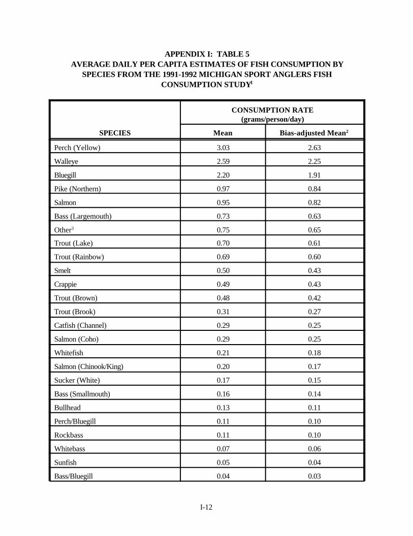
For the Great Lakes Water Quality Initiative a consumption survey by West et al. (1993)was used to characterize the consumption patterns of sport anglers in the Great LakesBasin (Table 5 of Appendix I). This study was selected because it represented the largestconsumption survey of sport anglers in the Great Lakes Basin. In addition, it was possibleto determine the type and quantity of each species consumed.

Percent lipid data from the fish contaminant monitoring programs in Michigan, Wisconsin,Ohio, Indiana, New York and Minnesota provided lipid data for edible tissues (e.g.,muscle) of fish from each of the Great Lakes (Tables 1-3 of Appendix I). Most lipid dataare for skin-on fillets because skin-on fillets are the accepted tissue sample used by mostof the Great Lakes fish consumption advisory programs.

The report "Trophic Level and Exposure Analyses for Selected Piscivorous Birds andMammals" (EPA, 1995) was used along with professional judgement to determine thetrophic level of the fish species consumed by the sport anglers. Each consumed fishspecies was assigned to either trophic level 3 or trophic level 4 based on data from thereport and/or professional judgement.

The data from the West survey (1993) in conjunction with the data from the fish monitoringprograms and the report on trophic levels of various fish species were used to determineconsumption weighted mean percent lipid values for use in deriving human health BAFs. The total grams per day of each species consumed by sport anglers was multiplied by the

8

C fdw ' (ffd)(C

tw )

percent lipid value for that species to determine the grams of lipid consumed per day bysport anglers for that species. The grams of lipid consumed from all species weresummed and divided by the total grams of fish consumed from trophic level 3 and trophiclevel 4 fish to arrive at a consumption weighted mean percent lipid value for each trophiclevel. These percent lipid values are used to derive BAFs which are then utilized incalculating human health criteria. The mean values for use in deriving human health BAFsare 1.82 for trophic level 3 fish consumed and 3.10 for trophic level 4 fish consumed (Table6 of Appendix I). The values were not rounded to whole numbers because they areintermediate values that are used in the derivation of human health criteria.

For wildlife, an analysis of the most common prey species consumed by the fiverepresentative wildlife species used to derive wildlife criteria was conducted. The dataallowed only a gross determination of the type of species consumed by the fiverepresentative species and the percent of prey species consumed from each trophic level. The analysis did not allow a quantitative determination of the quantity of the prey speciesconsumed at each trophic level. Consequently, a consumption weighted percent lipidvalue similar to that derived for humans was not possible. Nonetheless, a percent lipidvalue for both trophic level 3 and trophic level 4 were estimated using whole fish lipid datafrom the U.S. Fish and Wildlife Service national contaminant biomonitoring program, theCanada Department of Fisheries and Oceans, the New York Department of EnvironmentalConservation, and the Michigan Department of Natural Resources (Table 4 of Appendix I). The trophic levels of the species consumed were determined using the data from thereport "Trophic Level and Exposure Analyses for Selected Piscivorous Birds andMammals" (EPA, 1995). The mean percent lipid values for wildlife for use in derivingwildlife BAFs are 6.46 for trophic level 3 prey species consumed and 10.31 for trophiclevel 4 prey species consumed (Table 7 of Appendix I). The values were not rounded towhole numbers because they are intermediate values that are used in the derivation ofwildlife criteria.

B. Bioavailability

Baseline BAFs and BCFs for organic chemicals, whether measured or predicted, shall bebased on the concentration of the chemical that is freely dissolved in the ambient water inorder to account for bioavailability. For the purposes of this guidance, the relationshipbetween the total concentration of the chemical in the water (i.e., that which is freelydissolved plus that which is sorbed to particulate organic carbon or to dissolved organiccarbon) to the freely dissolved concentration of the chemical in the ambient water shall becalculated using the following equation:

where: C fw

d = freely dissolved concentration of the organic chemical in the

9

fd'

1

1 %(DOC)(K

OW)

10% (POC)(KOW)

(5)

C tw ' C fd

w % POC @ Cpoc % DOC @ Cdoc(6)

ambient water.C t

w = total concentration of the organic chemical in the ambient water.ffd = fraction of the total chemical in the ambient water that is freely

dissolved.

1. Determination of the Fraction of the Chemical that is Freely Dissolved inWater

The fraction of the chemical that is freely dissolved in the water, ffd, can be determinedusing the following equation with the KOW for the chemical and the DOC and POC of thewater.

where: DOC = concentration of dissolved organic carbon, kg of organic carbon/Lof water.

KOW = octanol-water partition coefficient of the chemical.POC = concentration of particulate organic carbon, kg of organic

carbon/L of water.

2. Derivation of the Equation Defining ffd

Experimental investigations have shown that hydrophobic organic chemicals exist in waterin three phases, 1) the freely dissolved phase, 2) sorbed to suspended solids and 3)sorbed to dissolved organic matter (Hassett and Anderson (1979), Carter and Suffet(1982), Landrum et al. (1984), Gschwend and Wu (1985), McCarthy and Jimenez (1985),Eadie et al. (1990, 1992)). The total concentration of the chemical in water is the sum ofthe concentrations of the sorbed chemical and the freely dissolved chemical (Gschwendand Wu (1985) and Cook et al. (1993)):

where: C fw

d = concentration of freely dissolved chemical in the ambient water,kg of chemical/L of water.

C tw = total concentration of the chemical in the ambient water, kg of

chemical/L of water.Cpoc = concentration of chemical sorbed to the particulate organic

carbon. in the ambient water, kg of chemical/kg of organic carbon.Cdoc = concentration of chemical sorbed to the dissolved organic carbon

10

tw ' C fd

w @ (1 % POC @ Kpoc % DOC @ Kdoc (7)

Kpoc 'Cpoc

C fdw

and Kdoc 'Cdoc

C fdw

(8)

ffd

'C fdw

C wt

(9)

fd'

11 % (DOC)(K

doc) % (POC)(K

poc) (10)

in the ambient water, kg of chemical/kg of organic carbon.POC = concentration of particulate organic carbon in the ambient water,

kg of organic carbon/L of water.DOC = concentration of dissolved organic carbon in the ambient water,

kg of organic carbon/L of water.

The above equation can also be expressed using partitioning relationships as:

where:

Kpoc = equilibrium partition coefficient of the chemical between POC andthe freely dissolved phase in the ambient water

Kdoc = equilibrium partition coefficient of the chemical between DOC andthe freely dissolved phase in the ambient water.

From equation 7, the fraction of the chemical which is freely dissolved in the water can becalculated using the following equations:

11

Kdoc .KOW

10(11)

Kpoc

. KOW (12)

fd'

1

1 %(DOC)(K

OW)

10% (POC)(KOW)

(13)

Experimental investigations by Eadie et al. (1990, 1992), Landrum et al. (1984), Yin andHassett (1986, 1989), Chin and Gschwend (1992), and Herbert et al. (1993) have shownthat Kdoc is directly proportional to the KOW of the chemical and is less than the KOW. TheKdoc can be estimated using the following equation:

The above equation is based upon the results of Yin and Hassett (1986, 1989), Chin andGschwend (1992), and Herbert et al. (1993). These investigations were done usingunbiased methods, such as the dynamic headspace gas-partitioning (sparging) and thefluorescence methods, for determining the Kdoc.

Experimental investigations by Eadie at al. (1990, 1992) and Dean et al. (1993) haveshown that Kpoc is approximately equal to the KOW of the chemical. The Kpoc can beestimated using the following equation:

By substituting equations 11 and 12 into equation 10 , the following equation is obtained:

C. Bioconcentration and Octanol-Water Partitioning

Numerous investigations have demonstrated a linear relationship between the logarithm ofthe bioconcentration factor (BCF) and the logarithm of the octanol-water partitioncoefficient (KOW) for organic chemicals for fish and other aquatic organisms. Isnard andLambert (1988) listed various regression equations that illustrate this linear relationship. The underlying assumption for the linear relationship between the BCF and KOW is that thebioconcentration process can be viewed as a partitioning of a chemical between the lipidsof the aquatic organisms and water and that the KOW is an useful surrogate for thispartitioning process (Mackay (1982)).

The regression equations demonstrating the linear relationship between the logarithms ofthe BCF and KOW have been developed using organic chemicals which are slowly, if at all,metabolized by fishes or other aquatic organisms. For metabolizable chemicals, theregression equations developed between BCF and KOW for non-metabolizable chemicals

12

log BCF ' 1.00 log KOW

& 0.08 (14)

BCF fdR . KOW

(15)

in most cases predict BCFs which are larger than the laboratory-measured BCFs. Thelosses of the chemicals due to metabolism are not accounted for in the simple partitioningmodel (Baron (1990), de Wolf et al. (1992)).

Mackay (1982) presented a thermodynamic basis for the partitioning process forbioconcentration and in essence, the BCF on a lipid-normalized basis (and freelydissolved concentration of the chemical in the water) should be similar if not equal to theKOW for organic chemicals. Unfortunately, almost all of the reported regression equationshave used BCFs reported on a wet weight basis instead of lipid-normalized. Whenregression equations are constructed using BCFs reported on a lipid-normalized basis,regression equations are obtained which have slopes and intercepts which are notsignificantly different from one and zero, respectively. For example, de Wolf et al. (1992)adjusted the relationship reported by Mackay (1982) to a 100 percent lipid basis (lipidnormalized basis) and obtained the following relationship:

For chemicals with large log KOWs (i.e., greater than 6.0), reported BCFs are often notequal to the KOW for non-metabolizable chemicals. As discussed by Gobas et al. (1989),this non-equality between the BCF and KOW is not caused by a breakdown of the BCF-KOW

relationship but rather is caused by (1) not accounting for growth dilution which occurredduring the BCF determination, (2) using the total concentration of the chemical in the waterinstead of the bioavailable (freely dissolved) concentration of the chemical in calculatingthe BCF, (3) not allowing sufficient time in the exposure to achieve steady-state conditions,and (4) not correcting for elimination of the chemical into the feces. BCFs for non-metabolizable chemicals are equal to the KOW when the BCFs are reported on lipid-normalized basis, determined using the freely dissolved concentration of the chemical inthe exposure water, corrected for growth dilution, determined from steady-state conditionsor determined from accurate measurements of the chemical's uptake (k1) and elimination(k2) rate constants from and to the water, respectively, and determined using no solventcarriers in the exposure.

In the final Guidance, predicted BCFs are estimated using the following approximation:

where: BCFRfd = BCF reported on lipid-normalized basis using the freely dissolved

concentration of the chemical in the water.

This relationship is applicable to organic chemicals which are either slowly or notmetabolized by aquatic organisms and have KOWs greater than a 1000. For chemical withKOWs less than a 1000, a slightly different relationship is applicable for organic chemicals

13

because the portion of the chemical in the organism that is not associated with lipidbecomes significant relative to the associated with the lipid. Appendix C contains acomplete derivation of this relationship.

Equation 15 implicitly assumes that n-octanol is an appropriate surrogate for lipids inaquatic organisms. If n-octanol is not an appropriate surrogate for lipids, the slope andintercept of equation 14 will not be 1.0 and 0.0, respectively. The theoretical basis and theexperimental data presented by Mackay (1982) suggest that n-octanol is a veryreasonable surrogate for lipids.

Equation 15 is also supported by and consistent with the food-chain model of Gobas(1993). For the Gobas model, the BCFR

fd is equal to KOW when the growth rate of theorganisms and metabolism rate of the chemical by the organisms are set equal to zero. Itshould be noted that the model does not use the partitioning process described by Mackay(1982) for bioconcentration. Instead the food-chain model predicts the k1 and k2 rateconstants for the fishes and the bioconcentration factor is determined by dividing theuptake rate constant from water (k1) by the elimination rate constant to water (k2).

The above equation is also supported by and consistent with the equilibrium partitioningtheory being developed by EPA for the derivation of sediment quality criteria (Di Toro et al.1991). Both the sediment organic carbon-water equilibrium partition coefficient (µg ofchemical/Kg of organic carbon in the sediment)/(µg of freely dissolved chemical/L ofsediment pore water) (Ksoc or Koc) and the lipid/water equilibrium partition coefficient (µg ofchemical/Kg of lipid)/(µg of freely dissolved chemical/L of sediment pore water) (KL) havebeen demonstrated to be approximately equal to KOW for organic chemicals in sedimentsand benthic organisms, respectively.

D. Food-Chain Biomagnification

The importance of uptake of chemicals through the diet and the potential for a stepwiseincrease in bioaccumulation from one trophic level to the next in natural systems has beenrecognized for many years (Hamelink et al. 1971). This pathway, involving transfer of achemical in food through successive trophic levels, is called biomagnification. Manyresearchers have noted that the BAFs of some chemicals in nature exceed thebioconcentration factors measured in the laboratory or estimated by log KOW models (e.g.,Oliver and Niimi 1983, Oliver and Niimi 1988, Niimi 1985, Swackhammer and Hites1988). Chemicals exhibiting this phenomenon are typically highly lipophilic, have low watersolubilities, and are resistant to being metabolized by aquatic organisms (Metcalf et al.1975).

1. Food-Chain Multiplier

FCMs for organic chemicals were determined using the model of Gobas (1993). This

14

FCM 'BAF fd

R

KOW

(16)

model includes both benthic and pelagic food chains thereby incorporating exposures oforganisms to chemicals from both the sediment and the water column. With the model ofGobas (1993), disequilibrium between the concentrations of the chemicals in sedimentand the water column are included in the predicted BAFs and the FCM derived from thepredicted BAFs. The disequilibrium is accounted for by inputting the concentrations of thechemical in the sediment and water column to the model. Subsequently, the disequilibriumis incorporated into the pelagic and benthic food web pathways because the modelpredicts the chemical residues in benthic invertebrates by using equilibrium partitioningand in zooplankton by assuming that the BCF for zooplankton is equal to the KOW ofchemical after correction for lipid content. Chemical residues for all other organisms (e.g.,fishes) are determined from the rates of (1) chemical uptake from food and water, (2)depuration and excretion of the chemical, (3) dilution due to growth of the organism, and(4) metabolism. This model requires the specification of the food chain structure, feedingpreferences, temperature of the ecosystem, organic carbon content of the sediments,organism weights and lipid contents, and the rate of metabolism of the chemical. Becauserates of metabolism for bioaccumulative chemicals are not known, the rate of metabolismused in determining the FCMs was zero (i.e., no metabolism).

The model of Gobas (1993) does not predict FCMs but rather it predicts the BAF for eachspecies in the food chain. FCMs can be calculated from the predicted BAFs using thefollowing equation:

where: KOW = octanol-water partition coefficient. BAFf

Rd = BAF reported on a lipid-normalized basis using the freely

dissolved concentration of the chemical in water.

a. Data for the Model

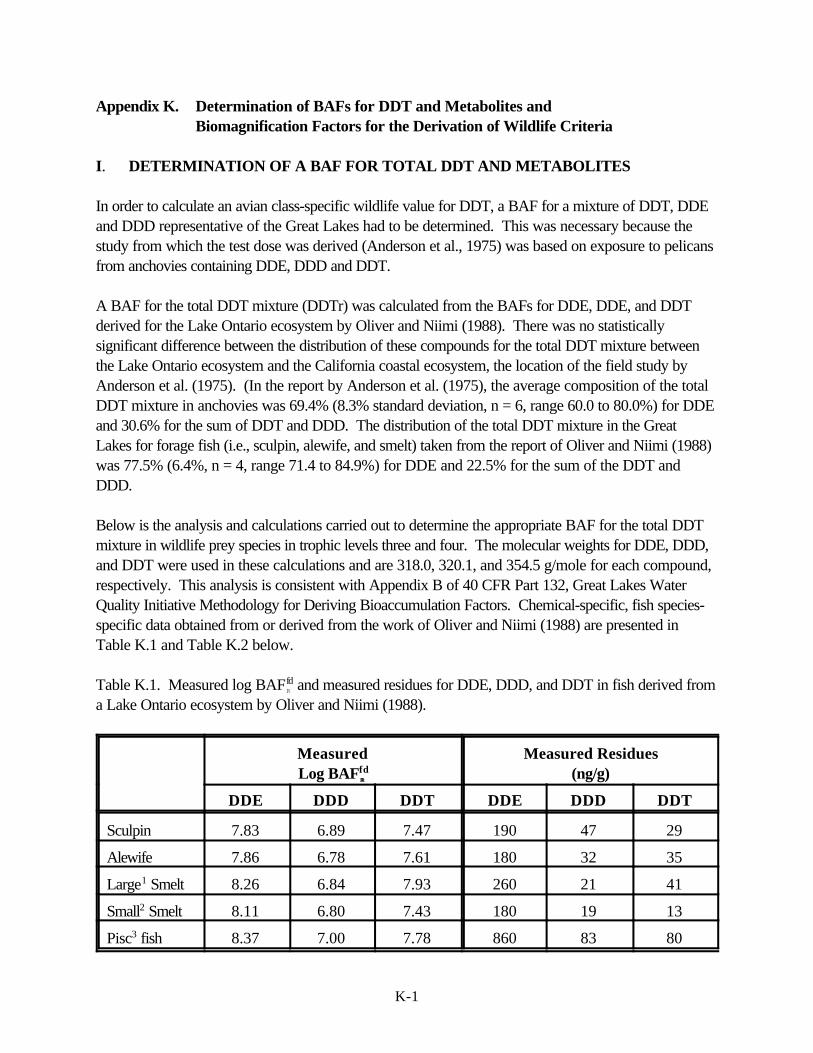
The data of Oliver and Niimi (1988) and Flint (1986) for Lake Ontario were used for thefeeding preferences, weights, and lipid contents for each species in the food chain (Table1). The mean water temperature of Lake Ontario was set to 8EC and the organic carboncontent of sediment was set to 2.7% as reported by Oliver and Niimi (1988) (Table 1). Values for the densities of the lipid and organic carbon were taken from Gobas (1993)(Table 1). The metabolic transformation rate constant was set equal to zero. The organiccarbon content of the water column was set to 0.0 kg/L (see b. Calculation of the FCMs).

With the values specified in Table 1, the remaining data needed for the model of Gobas(1993) are the concentrations of the chemical in the sediment and water column, and theKOW of the chemical. The KOW of the chemical is used as the independent variable in

15

of total chemical/Kg of organic carbon (infreely dissolved chemical/L of water(in water

fd'

11 % (DOC)(K

doc) % (POC)(K

poc) (17)

C fdw ' C t

w @ ffd(18)

deriving the FCMs and thus only the two chemical concentrations need to be defined forthe model.

To determine the relationship between the total concentration of the chemical in thesediment and the freely dissolved concentration of the chemical in the water column, thefollowing sediment-water column chemical concentration quotient (Asoc) was calculated foreach chemical reported by Oliver and Niimi (1988):

The freely dissolved concentrations of the chemicals in the water column were calculatedfrom the data of Oliver and Niimi (1988) using the equations of Gschwend and Wu (1985)and Cook et al. (1993). These equations are:

where: ffd = fraction of the chemical which is freely dissolved in the water;DOC = concentration of dissolved organic carbon;Kdoc = partition coefficient for the chemical between the DOC and the

freely dissolved phase in the water;POC = concentration of particulate organic carbon;Kpoc = partition coefficient for the chemical between the POC phase and

the freely dissolved phase in the water;Cw

f d = freely dissolved concentration of the chemical in the water;Cw

t = total concentration of the chemical in the water.

The concentrations in the water reported by Oliver and Niimi (1988) were obtained byliquid-liquid extraction of aliquots of Lake Ontario water which had passed through acontinuous-flow centrifuge to remove POC. Therefore, the concentrations in the waterreported by Oliver and Niimi (1988) include both the freely dissolved chemical and thechemical associated with the DOC in the water sample. The above equations were usedto derive the freely dissolved concentrations of the chemicals in the water by setting thePOC = 0.0 mg/L, DOC = 2 mg/L, and Kdoc = KOW/10. KOWs used to derive the freelydissolved concentrations are listed in Appendix B of this document. The relationship fordetermining Kdoc from KOW was developed from the results reported by Yin and Hassett

16

Csoc ' 25 @ KOW @ C fdw

(19)

(1986, 1989), Eadie et al. (1990, 1992), Landrum et al. (1984), and Herbert et al. (1993)for partitioning to DOC.

In Figure 1, the ratios of Asocw to KOW are plotted against the log KOW for each chemicalreported by Oliver and Niimi (1988). Visual inspection of Figure 1 suggest that the ratio ofAsocw to KOW is not strongly dependent upon the KOW. Correlation coefficients of the ratio(of Asocw to KOW) against log KOW of 0.02, -0.34, and -0.55 were obtained for the pesticides,PCB congeners, and the group of chemicals consisting of the chlorinated benzenes,toluenes, and butadienes, respectively. The average (standard deviation & number ofvalues) ratios for the Asocw to KOW for pesticides, PCB congeners, pesticides and PCBscombined, and the group of chemicals consisting of the chlorinated benzenes, toluenes,and butadienes were 11.8 (8.4 & 9), 25.9 (26.8 & 46), 23.6 (25.3 & 55), and 294 (1188 &12), respectively.

Based upon the independence of the ratios of Asocw to KOW on KOW for the pesticides andPCBs (the chemicals of primary concern in the derivation of food chain multipliers), a valueof 25 was selected for this ratio, the average of the pesticides and PCBs combined. Theresulting relationship between the concentration of the chemical in the sediment on anorganic carbon basis (Csoc) and the freely dissolved concentration of the chemical in thewater column (Cw

f d) is:

b. Calculation of the FCMs

The model of Gobas (1993) (MS-DOS version) was used to determine the FCMs. Alisting of the source code in FORTRAN is provided in Appendix J for the food web modelof Gobas (1993).

The model was run using the data listed in Table 1 with the above relationship (equation19) between the Csoc and Cw

f d for KOWs 3.5, 3.6, 3.7, 3.8, ..., and 9.0. The freely dissolvedconcentration of the chemical in the water was set to 1 ng/L and the concentration of thechemical in the sediment was calculated using the above sediment-water concentrationrelationship. The model of Gobas (1993) does not include solubility controls or limitations,and thus, the concentration of the chemical in the water used with the model is arbitrary fordetermining the BAFs (i.e., the BAF obtained using a 1 ng/L concentration of the chemicalwill be equal to that obtained using a 150 µg/L concentration of the chemical for aspecified KOW).

In using the model of Gobas (1993), we have not used his method for accounting forbioavailability. In section B of chapter III in this document, the procedure for determining

17

the freely dissolved concentration of the chemical in the ambient water is presented. Tonot use or override the method of Gobas for accounting for bioavailability, we have set theconcentration of the DOC in the model to an extremely small number, 1.0e-30 L/L. Themodel of Gobas (1993) takes the inputted total concentration of the chemical in the waterand before doing any predictions, corrects for bioavailability by calculating the freelydissolved concentration of the chemical in the water. The freely dissolved concentration ofthe chemical in the water is then used in all subsequent calculations by the model. Bysetting the concentration of the DOC to 1.0e-30 L/L, the total concentration of the chemicalinputted to the model becomes equal to the freely dissolved concentration of the chemicalin the water because the correction for bioavailability using the bioavailability method ofGobas is extremely small.

For each value of KOW inputted to the model, BAFfRds are reported by the model for each

organism in the food web. Using equation 16, FCMs were calculated for each organismusing the reported BAFf

Rds. Listed in Table 3 are the FCMs for trophic level 2

(zooplankton), trophic level 3 (forage fish), and trophic level 4 (piscivorous fish). The FCMsfor the forage fish, trophic level 3, were determined by taking the geometric mean of theFCMs for sculpin and alewife. The FCMs for the smelt were not used in determining themean FCMs for the forage fish because the diet of this organism includes small sculpin. This diet causes smelt to be at a trophic level slightly higher than 3 but less than trophiclevel 4. In contrast, the diets of the sculpin and alewife were solely trophic level 2organisms (i.e., zooplankton and Diporeia sp).

c. Application of FCMs

In the absence of a field-measured BAF or a predicted BAF derived from the BSAFmethodology, a FCM shall be used to calculate the baseline BAF for trophic levels 3 and 4from a laboratory-measured or predicted BCF. For an organic chemical, the FCM usedshall be derived from Table 3 using the chemical's log KOW and linear interpolation. AFCM greater than 1.0 applies to most organic chemicals with a log KOW of four or more. The trophic level used shall take into account the age or size of the fish species consumedby the human, avian or mammalian predator because, for some species of fish, the youngare in trophic level 3 whereas the adults are in trophic level 4.

The FCMs were developed assuming no metabolism of the chemical by any of theorganisms in the food web. Thus, for chemicals where metabolism is significant, thepredicted BAFs will be larger than a field-measured BAF or BAF determined using theBSAF methodology. BAFs predicted using laboratory-measured BCFs (i.e., the productof the FCM and the laboratory-measured BCF), might be in closer agreement with the fieldderived BAFs than the BAFs predicted using predicted BCFs because laboratory-measured BCFs might include some metabolism in their determination. In general, forhighly persistent chemicals, the effects of all metabolic processes can not be easilyincluded in the BCF determination.

18

The FCMs were determined using a disequilibrium factor of 25 from KOW (equation 16)between the concentrations of the chemical in the sediment on an organic carbonnormalized basis and the freely dissolved concentration of the chemical in water column. This disequilibrium is incorporated into the pelagic and benthic food web pathways in themodel of Gobas (1993) and is subsequently reflected in the BAFs predicted by the modeland the resulting FCMs.

d. Evaluation of FCMs

Baseline BAFs were predicted using the model of Gobas (1993) for each chemicalreported by Oliver and Niimi (1988). The predicted BAFs are equal to the product of theKOW and the FCM determined for that organism. Baseline BAFs also were derived fromthe data of Oliver and Niimi (1988) by dividing the lipid-normalized concentration of thechemical in the fish by the freely dissolved concentration of the chemical in the watercolumn. The freely dissolved concentration of the chemical in the water was determined asdescribed above. These results are summarized in Tables 3 through 8 and Figures 2through 7.

Measured chemical residues in fishes assigned to trophic level 3 can be higher than thosein trophic level 4 from the same food chain. Potential causes of the higher concentrations(on a lipid basis) in the trophic level 3 fish include (1) growth rates which are much slowerthan the predator fishes, and (2) differing rates of depuration and elimination of thechemical by the predator fishes.

The average differences between the predicted and measured log BAFs were -0.61, 0.01,-0.17, -0.04, -0.10, and -0.12 for zooplankton, sculpin, alewives, small smelt, large smelt,and piscivorous fish, respectively.

19

Table 1. Environmental Parameters and Species Characteristics Used with the Model ofGobas (1993) for Deriving the Food Chain Multipliers

Environmental parameters:Mean water temperature: 8ECOrganic carbon content of the sediment: 2.7%Organic carbon content of the water column: 1.0e-30 kg/LDensity of lipids: 0.9 kg/LDensity of organic carbon: 0.9 kg/LMetabolic transformation rate constant: 0.0 day-1

Species characteristics:Phytoplankton

Lipid content: 0.5%

Zooplankton: Mysids (Mysis relicta)Lipid content: 5.0%

Diporeia sp.Lipid content: 3.0%

Sculpin (Cottus cognatus)Lipid content: 8.0%Weight: 5.4 gDiet: 18% zooplankton, 82% Diporeia sp.

Alewives (Alosa pseudoharengus)Lipid content: 7.0%Weight: 32 gDiet: 60% zooplankton, 40% Diporeia sp.

Smelt (Osmerus mordax)Lipid content: 4.0%Weight: 16 gDiet: 54% zooplankton, 21% Diporeia sp., 25% sculpin

Salmonids (Salvelinus namaycush, Oncorhynchus mykiss, Oncorhynchus velinusnamaycush)

Lipid content: 11.0%Weight: 2410 gDiet: 10% sculpin, 50% alewives, 40% smelt

20

21

Table 2. Food-Chain Multipliers for Trophic Levels 2, 3 & 4.

Trophic Trophica TrophicLog KOW Level 2 Level 3 Level 4

2.0 1.000 1.005 1.0002.5 1.000 1.010 1.0023.0 1.000 1.028 1.0073.1 1.000 1.034 1.0073.2 1.000 1.042 1.0093.3 1.000 1.053 1.0123.4 1.000 1.067 1.0143.5 1.000 1.083 1.0193.6 1.000 1.103 1.0233.7 1.000 1.128 1.0333.8 1.000 1.161 1.0423.9 1.000 1.202 1.0544.0 1.000 1.253 1.0724.1 1.000 1.315 1.0964.2 1.000 1.380 1.1304.3 1.000 1.491 1.1784.4 1.000 1.614 1.2424.5 1.000 1.766 1.3344.6 1.000 1.950 1.4594.7 1.000 2.175 1.6334.8 1.000 2.452 1.8714.9 1.000 2.780 2.1935.0 1.000 3.181 2.6125.1 1.000 3.643 3.1625.2 1.000 4.188 3.8735.3 1.000 4.803 4.7425.4 1.000 5.502 5.8215.5 1.000 6.266 7.0795.6 1.000 7.096 8.5515.7 1.000 7.962 10.2095.8 1.000 8.841 12.0505.9 1.000 9.716 13.9646.0 1.000 10.556 15.9966.1 1.000 11.337 17.7836.2 1.000 12.064 19.9076.3 1.000 12.691 21.6776.4 1.000 13.228 23.281

22

6.5 1.000 13.662 24.604

23

Table 2. Continued.

Trophic Trophic TrophicLog KOW Level 2 Level 3 Level 4

6.6 1.000 13.980 25.6456.7 1.000 14.223 26.3636.8 1.000 14.355 26.6696.9 1.000 14.388 26.6697.0 1.000 14.305 26.2427.1 1.000 14.142 25.4687.2 1.000 13.852 24.3227.3 1.000 13.474 22.8567.4 1.000 12.987 21.0387.5 1.000 12.517 18.9677.6 1.000 11.708 16.7497.7 1.000 10.914 14.3887.8 1.000 10.069 12.0507.9 1.000 9.162 9.8408.0 1.000 8.222 7.7988.1 1.000 7.278 6.0128.2 1.000 6.361 4.5198.3 1.000 5.489 3.3118.4 1.000 4.683 2.3718.5 1.000 3.949 1.6638.6 1.000 3.296 1.1468.7 1.000 2.732 0.7788.8 1.000 2.246 0.5218.9 1.000 1.837 0.3459.0 1.000 1.493 0.226

a The FCMs for trophic level 3 are the geometric mean of the FCMs for sculpin andalewife.

24

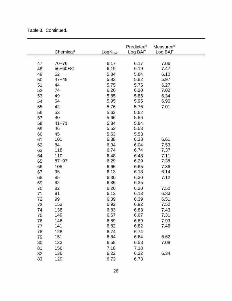
Table 3. Measured and Predicted BAFs for Zooplankton. BAFs are reported on a lipidweight basis using the freely dissolved concentration of the chemical in water (i.e., (µg ofchemical/Kg of lipid)/(µg of freely dissolved chemical/L of water)).

Predictedb Measuredc

Chemicala Log KOW Log BAF Log BAF

1 ppDDT 6.45 6.45 6.952 ppDDE 6.76 6.76 7.663 ppDDD 6.06 6.06 6.344 mirex 6.89 6.89 7.125 photomirex 6.89 6.89 7.356 g-chlordane 6.00 6.00 5.937 alpha-BHC 3.78 3.78 4.908 gamma-BHC 3.67 3.67 5.089 HCBD 4.84 4.84 5.05

10 OCS 6.29 6.29 6.7311 HCB 5.60 5.60 5.7612 QCB 5.11 5.11 6.3813 1,2,3,5-TeCB 4.65 4.65 5.3514 1,2,4,5-TeCB 4.56 4.56 5.1415 1,2,3,4-TeCB 4.59 4.59 5.3316 1,3,5-TCB 4.17 4.17 4.7117 1,2,4-TCB 3.99 3.99 4.9018 1,2,3-TCB 4.10 4.10 4.0719 2,4,5-TCT 4.93 4.9320 2,3,6-TCT 4.93 4.93 5.7121 PCT 6.36 6.3631 8 5.07 5.0732 6 5.06 5.0633 5 4.97 4.9734 12 5.22 5.2235 13 5.29 5.2936 28+31 5.67 5.67 6.4837 18 5.24 5.24 5.6938 22 5.58 5.58 6.2139 26 5.66 5.6640 16 5.16 5.1641 33 5.60 5.60 5.7942 17 5.25 5.25 5.6943 25 5.67 5.6744 24+27 5.40 5.4045 32 5.44 5.44

25

46 66 6.20 6.20 7.11

26

Table 3. Continued.


Chemicala LogKOW Log BAF Log BAF

47 70+76 6.17 6.17 7.0648 56+60+81 6.19 6.19 7.4749 52 5.84 5.84 6.1050 47+48 5.82 5.82 5.9751 44 5.75 5.75 6.2752 74 6.20 6.20 7.0253 49 5.85 5.85 6.3454 64 5.95 5.95 6.9655 42 5.76 5.76 7.0156 53 5.62 5.6257 40 5.66 5.6658 41+71 5.84 5.8459 46 5.53 5.5360 45 5.53 5.5361 101 6.38 6.38 6.6162 84 6.04 6.04 7.5363 118 6.74 6.74 7.3764 110 6.48 6.48 7.1165 87+97 6.29 6.29 7.3866 105 6.65 6.65 7.3667 95 6.13 6.13 6.1468 85 6.30 6.30 7.1269 92 6.35 6.3570 82 6.20 6.20 7.5071 91 6.13 6.13 6.3372 99 6.39 6.39 6.5173 153 6.92 6.92 7.5074 138 6.83 6.83 7.4375 149 6.67 6.67 7.3176 146 6.89 6.89 7.9377 141 6.82 6.82 7.4678 128 6.74 6.7479 151 6.64 6.64 6.6280 132 6.58 6.58 7.0881 156 7.18 7.1882 136 6.22 6.22 6.3483 129 6.73 6.73

27

84 180 7.36 7.36 7.66

28

Table 3. Continued.


Chemicala LogKOW Log BAF Log BAF

85 187+182 7.19 7.19 7.6086 170+190 7.37 7.37 8.2087 183 7.20 7.20 8.1688 177 7.08 7.08 8.0789 174 7.11 7.11 7.8890 178 7.14 7.1491 171 7.11 7.1192 185 7.11 7.1193 173 7.02 7.0294 203+196 7.65 7.65 8.2695 201 7.62 7.6296 194 7.80 7.80 7.6997 195 7.56 7.5698 198 7.62 7.6299 205 8.00 8.00

100 206 8.09 8.09101 207 7.74 7.74102 209 8.18 8.18

Average difference -0.61Standard deviation 0.39Number of values 61

a Chemical abbreviations taken from Oliver and Niimi(1988).b Predicted BAFs were obtained by taking the product of the FCM and KOW for each

chemical. Because the FCM is set to 1.0 for zooplankton, the predicted log BAFequals log KOW.

c Field-measured BAFs were determined by dividing the chemical residues on a lipidweight basis in the organisms (µg of chemical/Kg of lipid) by the freely dissolvedconcentration of thechemical in water (µg of freely dissolved chemical/L of water).

29

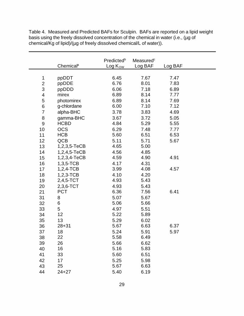
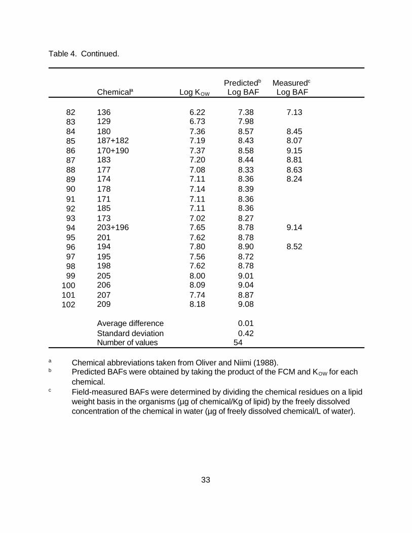
Table 4. Measured and Predicted BAFs for Sculpin. BAFs are reported on a lipid weightbasis using the freely dissolved concentration of the chemical in water (i.e., (µg ofchemical/Kg of lipid)/(µg of freely dissolved chemical/L of water)).



1 ppDDT 6.45 7.67 7.472 ppDDE 6.76 8.01 7.833 ppDDD 6.06 7.18 6.894 mirex 6.89 8.14 7.775 photomirex 6.89 8.14 7.696 g-chlordane 6.00 7.10 7.127 alpha-BHC 3.78 3.83 4.698 gamma-BHC 3.67 3.72 5.059 HCBD 4.84 5.29 5.55

10 OCS 6.29 7.48 7.7711 HCB 5.60 6.51 6.5312 QCB 5.11 5.71 5.6713 1,2,3,5-TeCB 4.65 5.0014 1,2,4,5-TeCB 4.56 4.8515 1,2,3,4-TeCB 4.59 4.90 4.9116 1,3,5-TCB 4.17 4.3117 1,2,4-TCB 3.99 4.08 4.5718 1,2,3-TCB 4.10 4.2019 2,4,5-TCT 4.93 5.4320 2,3,6-TCT 4.93 5.4321 PCT 6.36 7.56 6.4131 8 5.07 5.6732 6 5.06 5.6633 5 4.97 5.5134 12 5.22 5.8935 13 5.29 6.0236 28+31 5.67 6.63 6.3737 18 5.24 5.91 5.9738 22 5.58 6.4939 26 5.66 6.6240 16 5.16 5.8341 33 5.60 6.5142 17 5.25 5.9843 25 5.67 6.6344 24+27 5.40 6.19

30

45 32 5.44 6.23

31

Table 4. Continued.



46 66 6.20 7.36 7.4547 70+76 6.17 7.33 7.0648 56+60+81 6.19 7.35 7.4847 70+76 6.17 7.33 7.0648 56+60+81 6.19 7.35 7.4849 52 5.84 6.86 6.8050 47+48 5.82 6.84 6.1551 44 5.75 6.77 6.6552 74 6.20 7.36 7.3053 49 5.85 6.91 6.7754 64 5.95 7.05 7.1655 42 5.76 6.78 7.0756 53 5.62 6.5357 40 5.66 6.6258 41+71 5.84 6.8659 46 5.53 6.3860 45 5.53 6.3861 101 6.38 7.59 7.3062 84 6.04 7.14 8.0563 118 6.74 7.99 7.8664 110 6.48 7.71 7.4465 87+97 6.29 7.48 7.5466 105 6.65 7.90 7.8267 95 6.13 7.26 6.9868 85 6.30 7.49 7.5069 92 6.35 7.56 7.7070 82 6.20 7.36 7.6071 91 6.13 7.26 6.4472 99 6.39 7.6073 153 6.92 8.17 8.0574 138 6.83 8.08 8.0675 149 6.67 7.92 7.2876 146 6.89 8.14 8.4977 141 6.82 8.07 8.1178 128 6.74 7.9979 151 6.64 7.88 8.3480 132 6.58 7.82 7.41

32

81 156 7.18 8.42

33

Table 4. Continued.



82 136 6.22 7.38 7.1383 129 6.73 7.9884 180 7.36 8.57 8.4585 187+182 7.19 8.43 8.0786 170+190 7.37 8.58 9.1587 183 7.20 8.44 8.8188 177 7.08 8.33 8.6389 174 7.11 8.36 8.2490 178 7.14 8.3991 171 7.11 8.3692 185 7.11 8.3693 173 7.02 8.2794 203+196 7.65 8.78 9.1495 201 7.62 8.7896 194 7.80 8.90 8.5297 195 7.56 8.7298 198 7.62 8.7899 205 8.00 9.01

100 206 8.09 9.04101 207 7.74 8.87102 209 8.18 9.08

Average difference 0.01Standard deviation 0.42Number of values 54

a Chemical abbreviations taken from Oliver and Niimi (1988).b Predicted BAFs were obtained by taking the product of the FCM and KOW for each

chemical.c Field-measured BAFs were determined by dividing the chemical residues on a lipid

weight basis in the organisms (µg of chemical/Kg of lipid) by the freely dissolvedconcentration of the chemical in water (µg of freely dissolved chemical/L of water).

34

Table 5. Measured and Predicted BAFs for Alewives. BAFs are reported on a lipidweight basis using the freely dissolved concentration of the chemical in water (i.e., (µg ofchemical/Kg of lipid)/(µg of freely dissolved chemical/L of water)).



1 ppDDT 6.45 7.49 7.612 ppDDE 6.76 7.82 7.863 ppDDD 6.06 7.02 6.784 mirex 6.89 7.95 7.725 photomirex 6.89 7.95 7.636 g-chlordane 6.00 6.95 6.687 alpha-BHC 3.78 3.82 4.828 gamma-BHC 3.67 3.71 5.009 HCBD 4.84 5.22

10 OCS 6.29 7.31 7.7711 HCB 5.60 6.39 6.3112 QCB 5.11 5.6313 1,2,3,5-TeCB 4.65 4.9414 1,2,4,5-TeCB 4.56 4.8115 1,2,3,4-TeCB 4.59 4.8516 1,3,5-TCB 4.17 4.2917 1,2,4-TCB 3.99 4.0618 1,2,3-TCB 4.10 4.1819 2,4,5-TCT 4.93 5.3620 2,3,6-TCT 4.93 5.3621 PCT 6.36 7.39 6.5331 8 5.07 5.5932 6 5.06 5.5833 5 4.97 5.4334 12 5.22 5.8035 13 5.29 5.9236 28+31 5.67 6.51 6.6837 18 5.24 5.82 6.3938 22 5.58 6.3739 26 5.66 6.5040 16 5.16 5.7441 33 5.60 6.3942 17 5.25 5.8843 25 5.67 6.5144 24+27 5.40 6.09

35

45 32 5.44 6.13

36

Table 5. Continued.



46 66 6.20 7.20 7.5747 70+76 6.17 7.17 7.3148 56+60+81 6.19 7.19 7.7949 52 5.84 6.72 6.8450 47+48 5.82 6.70 6.8551 44 5.75 6.63 6.8652 74 6.20 7.20 7.3553 49 5.85 6.76 6.9854 64 5.95 6.90 7.3055 42 5.76 6.64 7.3856 53 5.62 6.4157 40 5.66 6.5058 41+71 5.84 6.7259 46 5.53 6.2760 45 5.53 6.2761 101 6.38 7.41 7.2562 84 6.04 6.99 7.9063 118 6.74 7.80 7.7164 110 6.48 7.53 7.5165 87+97 6.29 7.31 7.8966 105 6.65 7.71 7.7267 95 6.13 7.10 7.1468 85 6.30 7.32 7.6769 92 6.35 7.38 7.9370 82 6.20 7.20 7.8671 91 6.13 7.10 6.7472 99 6.39 7.42 7.3773 153 6.92 7.98 7.8274 138 6.83 7.89 7.8975 149 6.67 7.73 7.7576 146 6.89 7.95 8.3077 141 6.82 7.88 7.9678 128 6.74 7.8079 151 6.64 7.69 8.1780 132 6.58 7.63 7.4581 156 7.18 8.2382 136 6.22 7.22 7.25

37

83 129 6.73 7.79

38

Table 5. Continued.



84 180 7.36 8.38 8.1585 187+182 7.19 8.24 7.9986 170+190 7.37 8.39 8.8487 183 7.20 8.25 8.4688 177 7.08 8.13 8.5489 174 7.11 8.16 8.5190 178 7.14 8.1991 171 7.11 8.1692 185 7.11 8.1693 173 7.02 8.0894 203+196 7.65 8.59 8.8295 201 7.62 8.5996 194 7.80 8.71 8.2297 195 7.56 8.5398 198 7.62 8.5999 205 8.00 8.82

100 206 8.09 8.86101 207 7.74 8.68102 209 8.18 8.89





39

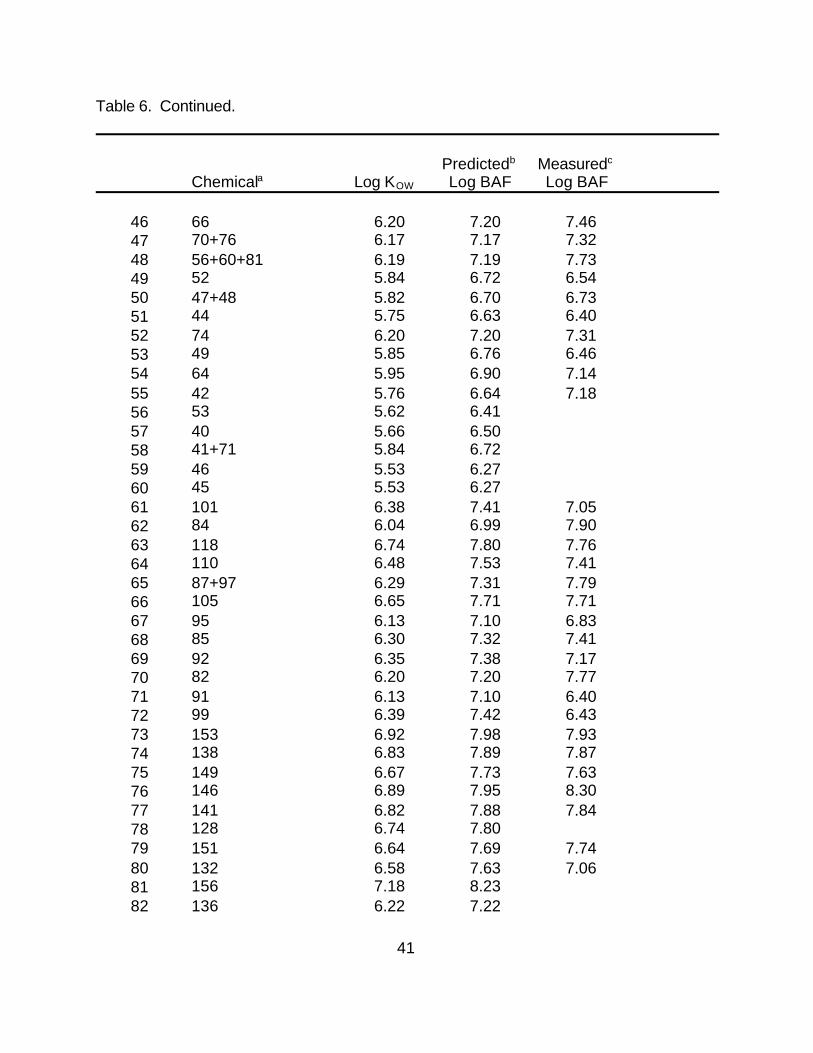
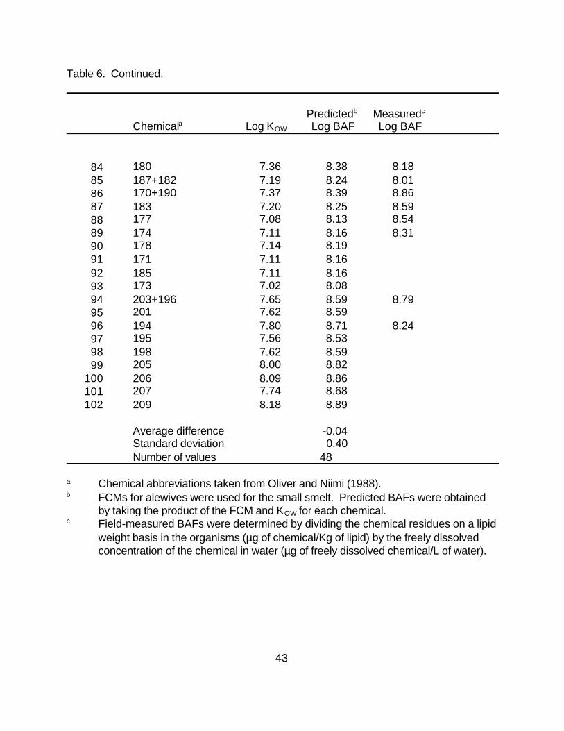
Table 6. Measured and Predicted BAFs for Small Smelt. BAFs are reported on a lipidweight basis using the freely dissolved concentration of the chemical in water (i.e., (µg ofchemical/Kg of lipid)/(µg of freely dissolved chemical/L of water)).




10 OCS 6.29 7.31 7.6111 HCB 5.60 6.39 6.1412 QCB 5.11 5.6313 1,2,3,5-TeCB 4.65 4.9414 1,2,4,5-TeCB 4.56 4.8115 1,2,3,4-TeCB 4.59 4.8516 1,3,5-TCB 4.17 4.2917 1,2,4-TCB 3.99 4.0618 1,2,3-TCB 4.10 4.1819 2,4,5-TCT 4.93 5.3620 2,3,6-TCT 4.93 5.3621 PCT 6.36 7.3931 8 5.07 5.5932 6 5.06 5.5833 5 4.97 5.4334 12 5.22 5.8035 13 5.29 5.9236 28+31 5.67 6.51 6.5737 18 5.24 5.8238 22 5.58 6.3739 26 5.66 6.5040 16 5.16 5.7441 33 5.60 6.3942 17 5.25 5.8843 25 5.67 6.5144 24+27 5.40 6.09

40

45 32 5.44 6.13

41

Table 6. Continued.



46 66 6.20 7.20 7.4647 70+76 6.17 7.17 7.3248 56+60+81 6.19 7.19 7.7349 52 5.84 6.72 6.5450 47+48 5.82 6.70 6.7351 44 5.75 6.63 6.4052 74 6.20 7.20 7.3153 49 5.85 6.76 6.4654 64 5.95 6.90 7.1455 42 5.76 6.64 7.1856 53 5.62 6.4157 40 5.66 6.5058 41+71 5.84 6.7259 46 5.53 6.2760 45 5.53 6.2761 101 6.38 7.41 7.0562 84 6.04 6.99 7.9063 118 6.74 7.80 7.7664 110 6.48 7.53 7.4165 87+97 6.29 7.31 7.7966 105 6.65 7.71 7.7167 95 6.13 7.10 6.8368 85 6.30 7.32 7.4169 92 6.35 7.38 7.1770 82 6.20 7.20 7.7771 91 6.13 7.10 6.4072 99 6.39 7.42 6.4373 153 6.92 7.98 7.9374 138 6.83 7.89 7.8775 149 6.67 7.73 7.6376 146 6.89 7.95 8.3077 141 6.82 7.88 7.8478 128 6.74 7.8079 151 6.64 7.69 7.7480 132 6.58 7.63 7.0681 156 7.18 8.2382 136 6.22 7.22

42

83 129 6.73 7.79

43

Table 6. Continued.



84 180 7.36 8.38 8.1885 187+182 7.19 8.24 8.0186 170+190 7.37 8.39 8.8687 183 7.20 8.25 8.5988 177 7.08 8.13 8.5489 174 7.11 8.16 8.3190 178 7.14 8.1991 171 7.11 8.1692 185 7.11 8.1693 173 7.02 8.0894 203+196 7.65 8.59 8.7995 201 7.62 8.5996 194 7.80 8.71 8.2497 195 7.56 8.5398 198 7.62 8.5999 205 8.00 8.82

100 206 8.09 8.86101 207 7.74 8.68102 209 8.18 8.89

Average difference -0.04 Standard deviation 0.40 Number of values 48

a Chemical abbreviations taken from Oliver and Niimi (1988).b FCMs for alewives were used for the small smelt. Predicted BAFs were obtained

by taking the product of the FCM and KOW for each chemical.c Field-measured BAFs were determined by dividing the chemical residues on a lipid


44

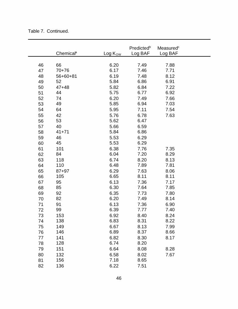
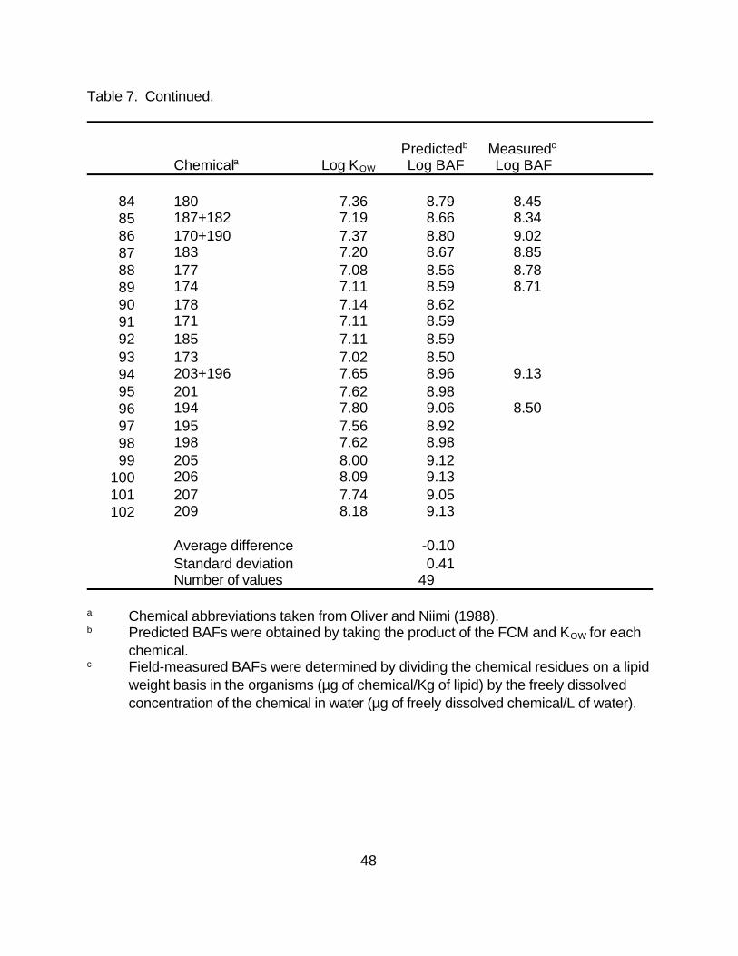
Table 7. Measured and Predicted BAFs for Large Smelt. BAFs are reported on a lipidweight basis using the freely dissolved concentration of the chemical in water (i.e., (µg ofchemical/Kg of lipid)/(µg of freely dissolved chemical/L of water)).




10 OCS 6.29 7.62 7.8511 HCB 5.60 6.45 6.4012 QCB 5.11 5.55 5.8713 1,2,3,5-TeCB 4.65 4.8514 1,2,4,5-TeCB 4.56 4.7215 1,2,3,4-TeCB 4.59 4.7716 1,3,5-TCB 4.17 4.2417 1,2,4-TCB 3.99 4.0318 1,2,3-TCB 4.10 4.1519 2,4,5-TCT 4.93 5.2620 2,3,6-TCT 4.93 5.2621 PCT 6.36 7.7231 8 5.07 5.5232 6 5.06 5.5133 5 4.97 5.3534 12 5.22 5.7435 13 5.29 5.8836 28+31 5.67 6.60 6.9237 18 5.24 5.7638 22 5.58 6.4339 26 5.66 6.5940 16 5.16 5.6841 33 5.60 6.4542 17 5.25 5.8443 25 5.67 6.6044 24+27 5.40 6.07

45

45 32 5.44 6.11

46

Table 7. Continued.



46 66 6.20 7.49 7.8847 70+76 6.17 7.46 7.7148 56+60+81 6.19 7.48 8.1249 52 5.84 6.86 6.9150 47+48 5.82 6.84 7.2251 44 5.75 6.77 6.9252 74 6.20 7.49 7.6653 49 5.85 6.94 7.0354 64 5.95 7.11 7.5455 42 5.76 6.78 7.6356 53 5.62 6.4757 40 5.66 6.5958 41+71 5.84 6.8659 46 5.53 6.2960 45 5.53 6.2961 101 6.38 7.76 7.3562 84 6.04 7.20 8.2963 118 6.74 8.20 8.1364 110 6.48 7.89 7.8165 87+97 6.29 7.63 8.0666 105 6.65 8.11 8.1167 95 6.13 7.36 7.1768 85 6.30 7.64 7.8569 92 6.35 7.73 7.8070 82 6.20 7.49 8.1471 91 6.13 7.36 6.9072 99 6.39 7.77 7.4073 153 6.92 8.40 8.2474 138 6.83 8.31 8.2275 149 6.67 8.13 7.9976 146 6.89 8.37 8.6677 141 6.82 8.30 8.1778 128 6.74 8.2079 151 6.64 8.08 8.2880 132 6.58 8.02 7.6781 156 7.18 8.6582 136 6.22 7.51

47

83 129 6.73 8.19

48

Table 7. Continued.



84 180 7.36 8.79 8.4585 187+182 7.19 8.66 8.3486 170+190 7.37 8.80 9.0287 183 7.20 8.67 8.8588 177 7.08 8.56 8.7889 174 7.11 8.59 8.7190 178 7.14 8.6291 171 7.11 8.5992 185 7.11 8.5993 173 7.02 8.5094 203+196 7.65 8.96 9.1395 201 7.62 8.9896 194 7.80 9.06 8.5097 195 7.56 8.9298 198 7.62 8.9899 205 8.00 9.12

100 206 8.09 9.13101 207 7.74 9.05102 209 8.18 9.13





49

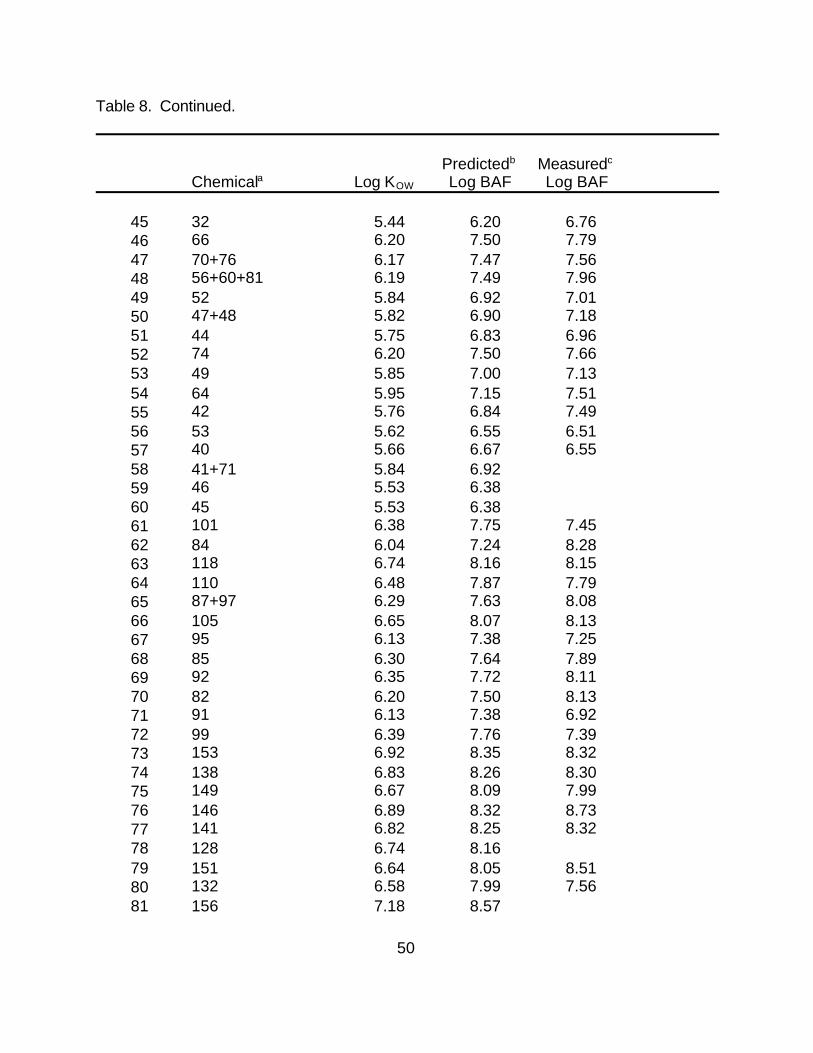
Table 8. Measured and Predicted BAFs for Piscivorous Fish. BAFs are reported on alipid weight basis using the freely dissolved concentration of the chemical in water (i.e., (µgof chemical/Kg of lipid)/(µg of freely dissolved chemical/L of water)).




10 OCS 6.29 7.62 8.0711 HCB 5.60 6.53 6.4012 QCB 5.11 5.61 5.8113 1,2,3,5-TeCB 4.65 4.8514 1,2,4,5-TeCB 4.56 4.7015 1,2,3,4-TeCB 4.59 4.75 5.0716 1,3,5-TCB 4.17 4.2217 1,2,4-TCB 3.99 4.0118 1,2,3-TCB 4.10 4.1319 2,4,5-TCT 4.93 5.3020 2,3,6-TCT 4.93 5.3021 PCT 6.36 7.7131 8 5.07 5.5832 6 5.06 5.5733 5 4.97 5.3834 12 5.22 5.8135 13 5.29 5.9636 28+31 5.67 6.68 6.8937 18 5.24 5.83 5.7538 22 5.58 6.51 6.3939 26 5.66 6.6740 16 5.16 5.75 5.9241 33 5.60 6.53 5.3242 17 5.25 5.92 5.5243 25 5.67 6.6844 24+27 5.40 6.16

50

Table 8. Continued.



45 32 5.44 6.20 6.7646 66 6.20 7.50 7.7947 70+76 6.17 7.47 7.5648 56+60+81 6.19 7.49 7.9649 52 5.84 6.92 7.0150 47+48 5.82 6.90 7.1851 44 5.75 6.83 6.9652 74 6.20 7.50 7.6653 49 5.85 7.00 7.1354 64 5.95 7.15 7.5155 42 5.76 6.84 7.4956 53 5.62 6.55 6.5157 40 5.66 6.67 6.5558 41+71 5.84 6.9259 46 5.53 6.3860 45 5.53 6.3861 101 6.38 7.75 7.4562 84 6.04 7.24 8.2863 118 6.74 8.16 8.1564 110 6.48 7.87 7.7965 87+97 6.29 7.63 8.0866 105 6.65 8.07 8.1367 95 6.13 7.38 7.2568 85 6.30 7.64 7.8969 92 6.35 7.72 8.1170 82 6.20 7.50 8.1371 91 6.13 7.38 6.9272 99 6.39 7.76 7.3973 153 6.92 8.35 8.3274 138 6.83 8.26 8.3075 149 6.67 8.09 7.9976 146 6.89 8.32 8.7377 141 6.82 8.25 8.3278 128 6.74 8.1679 151 6.64 8.05 8.5180 132 6.58 7.99 7.5681 156 7.18 8.57

51

82 136 6.22 7.52 7.37

52

Table 8. Continued.



83 129 6.73 8.1584 180 7.36 8.68 8.5885 187+182 7.19 8.58 8.4386 170+190 7.37 8.69 9.2087 183 7.20 8.59 9.0388 177 7.08 8.49 9.0189 174 7.11 8.52 8.7490 178 7.14 8.5591 171 7.11 8.5292 185 7.11 8.5293 173 7.02 8.4494 203+196 7.65 8.81 9.2695 201 7.62 8.8496 194 7.80 8.88 8.5697 195 7.56 8.7898 198 7.62 8.8499 205 8.00 8.89

100 206 8.09 8.87101 207 7.74 8.90102 209 8.18 8.83





53

54

55

56

57

58

59

60

BSAF .C fdb ·KR

C fds ·Ksoc

' Dbs·

KR

Ksoc

. Dbs@ 2 (21)

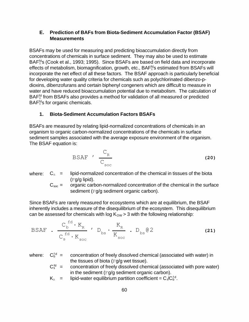
E. Prediction of BAFs from Biota-Sediment Accumulation Factor (BSAF)Measurements

BSAFs may be used for measuring and predicting bioaccumulation directly fromconcentrations of chemicals in surface sediment. They may also be used to estimateBAFf

Rds (Cook et al., 1993; 1995). Since BSAFs are based on field data and incorporate

effects of metabolism, biomagnification, growth, etc., BAFfRds estimated from BSAFs will

incorporate the net effect of all these factors. The BSAF approach is particularly beneficialfor developing water quality criteria for chemicals such as polychlorinated dibenzo-p-dioxins, dibenzofurans and certain biphenyl congeners which are difficult to measure inwater and have reduced bioaccumulation potential due to metabolism. The calculation ofBAFf

Rd from BSAFs also provides a method for validation of all measured or predicted

BAFfRds for organic chemicals.

1. Biota-Sediment Accumulation Factors BSAFs

BSAFs are measured by relating lipid-normalized concentrations of chemicals in anorganism to organic carbon-normalized concentrations of the chemicals in surfacesediment samples associated with the average exposure environment of the organism. The BSAF equation is:

BSAF 'CR

Csoc

(20)

where: CR = lipid-normalized concentration of the chemical in tissues of the biota(Fg/g lipid).

Csoc = organic carbon-normalized concentration of the chemical in the surfacesediment (Fg/g sediment organic carbon).

Since BSAFs are rarely measured for ecosystems which are at equilibrium, the BSAFinherently includes a measure of the disequilibrium of the ecosystem. This disequilibriumcan be assessed for chemicals with log KOW > 3 with the following relationship:

where: C fb

d = concentration of freely dissolved chemical (associated with water) inthe tissues of biota (Fg/g wet tissue).

C fsd = concentration of freely dissolved chemical (associated with pore water)

in the sediment (Fg/g sediment organic carbon).KR = lipid-water equilibrium partition coefficient = CR/Cb

f d.

61

(BAF fdR )i '

(CR)i

(C fdw )

i

(22)

Ksoc = the sediment organic carbon-water equilibrium partition coefficient =Csoc/Cs

fd.Dbs = the disequilibrium (fugacity) ratio between biota and sediment

(Cbf d/Cs

fd).

Measured BSAFs may range widely for different chemicals depending on KR, Ksoc, and theactual ratio of C f

bd to C f

sd. At equilibrium, which rarely exists between sediment and pelagic

organisms such as fish, the BSAF would be expected to equal the ratio of KR/Ksoc which isthought to range from 1-4. When chemical equilibrium between sediment and biota doesnot exist, the BSAF will equal the disequilibrium (fugacity) ratio between biota andsediment (Dbs = C f

bd/C f

sd) times the ratio of the equilibrium partition coefficients

(approximately 2).

The deviation of Dbs from the equilibrium value of 1.0 is determined by the net effect of allfactors which contribute to the disequilibrium between sediment and aquatic organisms. Dbs > 1 can occur due to biomagnification or when surface sediment has not reachedsteady-state with water. Dbs < 1 can occur as a result of kinetic limitations for chemicaltransfer from sediment to water or water to food chain, and biological processes, such asgrowth or biotransformation of the chemical in the animal and its food chain. BSAFs aremost useful when measured under steady-state conditions or pseudo-steady-stateconditions in which chemical concentrations in water are linked to slowly changingconcentrations in sediment. BSAFs measured for systems with new chemical loadings orrapid increases in loading may be unreliable due to underestimation of steady-state Csocs.

2. Relationship of BAFs to BSAFs

Differences between BSAFs for different organic chemicals are good measures of therelative bioaccumulation potentials of the chemicals. When calculated from a commonorganism/sediment sample set, chemical-specific differences in BSAFs reflect primarilythe net effect of biomagnification, metabolism, and bioenergetic and bioavailability factorson each chemical's Dbs. Ratios of BSAFs of PCDDs and PCDFs to a BSAF for TCDD(bioaccumulation equivalency factors, BEFs) have been proposed in the GLWQI forevaluation of TCDD toxic equivalency associated with complex mixtures of thesechemicals (see 58 FR 20802). The same approach is applicable to calculation of BAFsfor other organic chemicals. The approach requires data for a steady-state or nearsteady-state condition between sediment and water for both a reference chemical (r) witha field-measured BAFf

Rd and other chemicals (n=i) for which BAFf

Rds are to be determined.

BAFfRd for a chemical "i" is defined as:

62

(Asoc)i '(C

soc)i

(C fdw )

i

(24)

(BAF fdR )i

(BAF fdR )r

'(BSAF)i(Asoc)i(BSAF)

r(A

soc)r

(25)

(BAF fdR )i ' (BAF fd

R )r ·(BSAF)

i(K

OW)i

(BSAF)r(K

OW)r

(27)

where: CR = lipid-normalized concentration of the chemical in tissues of the biota(Fg/g lipid).

C fw

d = concentration of freely dissolved chemical in water (Fg/FL water).

Substitution of CR from equation 20 into CR of equation 22 for the chemical i gives:

(BAF fdR )i ' (BSAF)i @

(Csoc)i

(C fdw )

i

(23)

In order to avoid confusion with the equilibrium partition coefficients Ksoc, Kpoc or Kdoc, thechemical concentration quotient between sediment organic carbon and a freely dissolvedstate in overlying water is symbolized by Asoc:

Thus the ratio of BAFfRd for chemical i and a reference chemical r is:

If both chemicals have similar fugacity ratios between water and sediment, as is the casefor many chemicals in the open waters of the Great Lakes:

(Asoc)i

(Asoc)r

'(K

OW)i

(KOW)r

(26)

therefore:

The assumption of equal or similar fugacity ratios between water and sediment for eachchemical is equivalent to assuming that for all chemicals used in BAFf

Rd calculations: (1)

the concentration ratios between sediment and suspended solids in the water and (2) thedegree of equilibrium between suspended solids and Cw

f d are the same. Thus, errorscould be introduced by inclusion of chemicals with non-steady-state external loading ratesor chemicals with strongly reduced Cw

f d due to rapid volatilization from the water. Note that

63

BAFfRds calculated from BSAFs will incorporate any errors associated with measurement of

the BAFfRd for the reference chemical and the KOWs for both the reference and unknown

chemicals. Such errors can be minimized by comparing results from several referencechemicals, including those with similar KOWs to those of the unknown chemicals, and byassuring consistent use of Cw

f d values which are adjusted for dissolved organic carbonbinding effects on the fraction of each chemical that is freely dissolved (ffd) in unfiltered,filtered or centrifuged water samples. BAFRs based on total chemical concentration inwater (BAFR

t) can be calculated on the basis of ffd for the dissolved and particulate organiccarbon concentrations in the water (POC and DOC):

BAF tR ' BAF fd

R @ffd(28)

where:

'1

1 % DOC @Kdoc % POC @Kpoc

. 1

1 %DOC @KOW

10% POC

(29)

Further information on calculation of concentrations of freely dissolved chemicals in watermay be found in section III.B of this document titled "Bioavailability".

3. Calculation of BAF fRRds from Lake Ontario Data

Two data sets are available to EPA for calculating BAFfRds from BSAFs for fish in Lake

Ontario. The Oliver and Niimi (1988) data set, which has been used extensively forconstruction of food chain models of bioaccumulation and calculation of FCMs,biomagnification factors and BAFf

Rds from chemical concentrations determined in

organisms and water, also contains surface sediment data which allows calculation oflakewide average BSAFs. The second data set is provided by an extensive sampling offish and sediments in 1987 for EPA's Lake Ontario TCDD Bioaccumulation Study (U.S.EPA, 1990) for the purpose of determining BSAFs. These samples were later analyzedfor PCDD, PCDF, PCB congeners and some organochlorine pesticides at ERL-Duluth. Although these data should be submitted for publication within this year, they are neededhere to provide a unique data set for checking BAFf

Rds calculated from Oliver and Niimi

data from samples collected between 1981-1984 and calculating BAFfRds for organic

chemicals not measured by Oliver and Niimi.

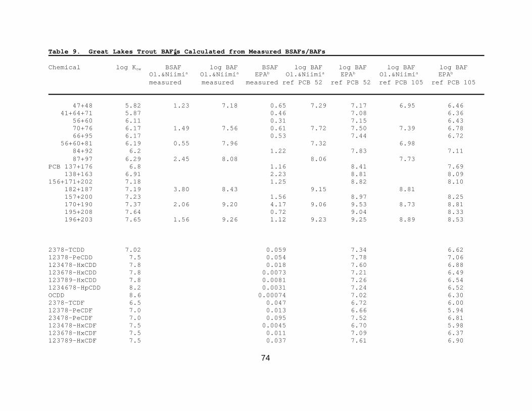
BAFfRds for salmonids were calculated for this demonstration of the BSAF ratio method

using PCB congeners 52, 105 and 118 and DDT as reference chemicals. Severalreference chemicals were used in order to examine the variability introduced by choice ofreference chemical. The water analyses of Oliver and Niimi (1988) were adjusted for anestimated 2 mg/L residual dissolved organic carbon concentration in the centrifuged water(assumed no residual POC) and an estimated Kdoc = KOW/10 in order to calculate Cw

f d fromffd (equation 30). Log KOWs for PCBs are those reported by Hawker and Connell (1988).

64

Log KOWs for PCDDs and PCDFs are those estimated by Burkhard and Kuehl (1986)except for the penta, hexa, and hepta chlorinated dibenzofurans which were estimated onthe basis of assumed similarity to the trends reported for the PCDDs by Burkhard andKuehl (1986). Log KOWs for other chemicals are either as cited in the Appendix B of thisdocument or noted in Table 9. Table 9 contains the measured and predicted log BAFf

Rds

from the two data sets.

4. Validity of BAF fRRds Calculated from BSAFs

Figures 8, 9, and 10 show the relationship of log BAFfRds to log KOWs for (1) Oliver and

Niimi (1988) BAFfRds determined from measured concentrations of freely dissolved

chemicals in Lake Ontario water in 1984; (2) BAFfRds calculated from BSAFs derived from

Oliver and Niimi data; and (3) BAFfRds calculated from EPA BSAFs for lake trout in Lake

Ontario in 1987 (Cook et al., 1995). The diagonal lines represent a 1:1 ratio of log BAF tolog KOW. The PCB congener BAFf

Rds in all three sets of data appear quite similar. The

EPA BAFfRds predictions (figure 3) include a number of chemicals not in the Oliver and

Niimi data set. These are the PCDDs, PCDFs, chlordanes, nonachlors and dieldrin. Onlythe dieldrin BAFf

Rd has been measured elsewhere. The BAFf

Rds for five of six chlordanes

and nonachlors are much greater than those for PCBs with the same estimated log KOW. Therefore, the log KOW values chosen here for the chlordanes and nonachlors may besignificantly underestimated. The bioaccumulative PCDDs and PCDFs (2,3,7,8-chlorinated), as expected due to metabolism in fish, have BAFf

Rds 10-1000 fold less than

PCBs with similar KOWs. Thus, the BSAF method for measuring BAFfRds appears to work

well for Lake Ontario.

Accuracy of the BSAF method can be best judged on the basis of comparison of theBAFf

Rds calculated from BSAFs to field-measured BAFf

Rds. Figure 11 illustrates the

agreement between log BAFfRds calculated from the Oliver and Niimi water data and those

calculated from the sediment data. The BAFfRds for chlorinated benzenes and toluenes may

tend to be underestimated with BSAFs because the water-sediment fugacity gradient isaltered in comparison to PCBs in response to rapid volatilization losses from water. Useof EPA BSAFs measured from a different set of fish and sediment samples collectedseveral years after the Oliver and Niimi samples gives BAFf

Rds that correlate equally well

with the BAFfRds calculated from Oliver and Niimi data (figure 12).

All of the above correlations were based on the BSAF method using the Oliver and Niimimeasured Lake Ontario salmonid BAFf

Rd for PCB congener 52 as the reference. Very

similar correlations result for comparisons of data in Table 9 for PCB congeners 105, 118or DDT as reference chemicals. The BSAF method is strengthened through use of severalreference chemicals with a range of KOWs and greatest likelihood for accuracy inmeasurements of concentrations in water. The two data sets and four reference chemicalsresulted in either four or eight determinations of BAFf

Rd for each chemical listed in Table 9.

Mean log BAFfRds (geometric means of BAFf

Rds) for the 4-8 determinations from Lake

65

Ontario data are reported in Table 10. The BAFfRd for 2,3,7,8-tetrachlorodibenzo-p-dioxin

(TCDD) at 7.85 × 106 compares well to 3.03 × 106 estimated by a different method forTCDD log KOW = 7 by Cook et al. (1993). The small difference in the two estimates maybe attributable to an underestimate of the sediment-disequilibrium between sediment andwater by Cook et al. (1993) that resulted in an overestimate of Cw

f d.

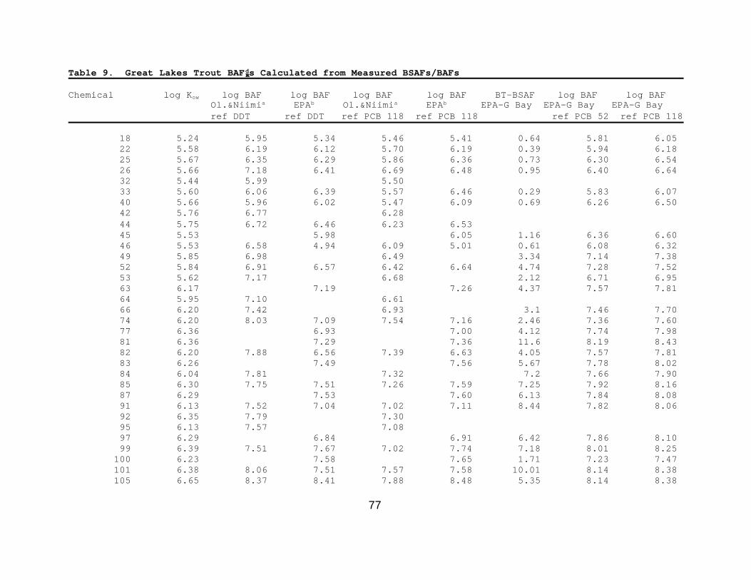
The greatest test for robustness of the BSAF method for predicting BAFfRds that are

applicable throughout the Great Lakes would be a comparison of two totally independentdata sets based on different ecosystems and conditions. Such a comparison can bemade for bioaccumulation of PCBs in Lake Ontario fish and Green Bay fish. The EPAGreen Bay/Fox River Mass Balance Study involved extensive sampling of water, sedimentand fish in 1989. Green Bay is a shallower, smaller, and more eutrophic body of waterthan Lake Ontario. Measurement of bioaccumulation in Green Bay is complicated by themovement and interaction of biota through gradients of decreasing PCBs, nutrients andsuspended organic carbon which extend from the Fox River to the outer bay and LakeMichigan. Table 9 contains brown trout BAFf

Rds calculated from PCB BSAFs measured in

the mid-bay region using PCB congeners 52 and 118 as reference chemicals. Thereference chemical BAFf

Rds were determined with water and brown trout data from the

same region. Concentrations of freely dissolved PCBs were calculated, as for LakeOntario, on the basis of dissolved organic carbon in the water samples and an assumedKdoc = KOW/10. Despite the complex exposures of Green Bay fish, figures 13 and 14illustrate log BAFf

Rd - log KOW relationships found in Green Bay which are similar to those

from the Oliver and Niimi and EPA Lake Ontario data sets. The correlations between thePCB BAFf

Rds for Green Bay brown trout and BAFf

Rds based on Oliver-Niimi salmonid and

water measurements and EPA lake trout BSAFs are shown in figures 15-18 for referencechemicals PCB 52 and PCB 118, respectively. Good agreement exists between GreenBay brown trout predictions and Lake Ontario measured and BSAF-predicted BAFf

Rds for

both reference chemicals.

The means of log BAFfRds calculated for each chemical from two sets of BSAFs and four

reference chemicals for 124 chemicals measured in Lake Ontario trout (Table 10) areplotted against log KOW in figure 19. Only 59 of these chemicals have field-measuredBAFf

Rds. Correlations between the mean Lake Ontario trout and Green Bay brown trout

BAFfRds (figures 20 and 21) indicate that the Green Bay brown trout may be slightly larger.

This may be a sample set artifact associated with the complex Green Bay fish-water-sediment relationships in Green Bay rather than an actual site/species/food chain-specificdifference in bioaccumulation. The agreement of the Green Bay and Lake Ontario resultsdemonstrates the general applicability of BAFf

Rds calculated from BSAFs in predicting

bioaccumulation in Great Lakes fish from estimated Cwf ds.

5. How to Apply the BSAF Method for Predicting BAF fRRds

If high quality data are not available for calculating BAFfRds for organic chemicals that are

66

expected to bioaccumulate, the mean BAFfRds reported in Table 10 may be used. To apply

the method for additional chemicals, site-specific determinations, or biota from differenttrophic levels than salmonids, the following steps and data requirements must becompleted:

a. Reliable BAFfRds which have been measured for several reference chemicals in

biota in the ecosystem must be chosen. The water sample analyses shouldapproximate the average exposure of the organism and its food chain over a timeperiod that is most appropriate for the chemical, organism and ecosystem. Each Cw

f d

used to calculate a BAFfRd should be based on a consistent adjustment of the

concentration of total chemical in water for DOC and POC using equation 30. It ispreferable to choose at least some reference chemicals on the basis of log KOW andchemical class similarity with the test chemicals.

b. Measured (slow-stir method or equivalent preferred) or estimated Log KOW valuesare chosen for each chemical.

c. Obtain chemical residue and % lipid data for representative samples of the tissuesof the organisms. Migration patterns, food chain movement and hydrodynamicfactors should be considered. For highly bioaccumulative chemicals variation ofchemical residues in adult fish in the open waters of the Great Lakes within an annualcycle is usually slight.

d. Obtain chemical concentrations and % organic carbon data for surface sedimentsamples. Sediment sampling sites should be selected to allow prediction of ratios offreely dissolved chemical concentrations in the overlying water of the ecosystemregion of interest. A 1 cm layer of surface sediment is ideal but 3 cm samples willwork if sedimentation rates are large and periodic scouring events are not likely. Although desirable, sediment samples do not have to represent the average surfacesediment condition in the area of the ecosystem affecting the exposure of theorganisms for which bioaccumulation is to measured. Since this is a ratio method,the concentrations of each chemical in sediment need only be predictive of the ratiosof concentrations of the chemicals in the ecosystem water.

e. With the data from steps 3 and 4, calculate BSAFs for chemicals of interest andreference chemicals (equation 21).

f. With BSAFs and KOWs for each chemical, plus BAFfRds for reference chemicals,

calculate BAFfRds using equation 27.

g. Use the BAFfRds to predict chemical residues in fish and other biota or to establish

unsafe concentrations of chemicals in water only on the basis of chemicalconcentration expressions for water and organisms that are consistent with the BAFf

Rd

67

definition and measurement.

6. Summary

BAFfRds calculated from two different BSAF data sets for Lake Ontario salmonids are

similar and agree well with field-measured BAFfRds of Oliver and Niimi (1988). The BSAF

method allows calculation of BAFfRds for chemicals which have not been measured in Great

Lakes water but are detectable in fish tissues and sediments. BAFfRds can also be

calculated for other fish species and biota at lower trophic levels in the food web. BAFfRds

calculated for PCBs in Green Bay brown trout agree well with the Lake Ontariosalmonid/lake trout values despite differences in ecosystem, food chain and exposureconditions. Mean log BAFf

Rds (geometric mean of BAFf

Rds) from 4-8 determinations from

Lake Ontario data are summarized in Table 10.

68

Table 9. Great Lakes Trout BAF RRds Calculated from Measured BSAFs/BAFs.

Chemical log Kow BSAF log BAF BSAF log BAF log BAF log BAF log BAF Ol.&Niimia Ol.&Niimia EPAb Ol.&Niimia EPAb Ol.&Niimia EPAb measured measured measured ref PCB 52 ref PCB 52 ref PCB 105 ref PCB 105

dieldrin 5.3 6.65 7.67 6.95ddt 6.45 1.09 7.78 1.67 7.87 8.22 7.54 7.50dde 6.76 4.14 8.35 7.7 8.76 9.19 8.43 8.47ddd 6.06 0.28 7.00 6.90 6.56mirex 6.89 1.43 8.13 1.31 8.43 8.55 8.09 7.84photomirex 6.89 5.48 8.07 9.01 8.68g-chlordane 6.0 2.22 6.79 7.73 7.40t-chlordane 6.0 2.00 7.85 7.13c-chlordane 6.0 4.77 8.23 7.51t-nonachlor 6.0 10.5 8.57 7.85c-nonachlor 6.0 0.51 7.25 6.54alpha-hch 3.78 2.45 4.69 5.55 5.22gamma-hch 3.67 0.69 4.93 4.89 4.56hcbd 4.84ocs 6.29 0.98 8.07 7.67 7.33hcb 5.6 0.09 6.40 5.95 5.62pcb 5.11 0.04 5.81 5.07 4.731235tcb 4.561245tcb 4.561234tcb 4.59 0.01 5.07 4.11 3.78135tcb 4.17124tcb 3.99123tcb 4.1 245tct 4.93236tct 4.93pct 6.36

total-PCB 6.14 1.85 7.81 7.79 7.46 PCBs 5 4.97 6 5.06 0.36 6.16 5.44 8 5.07

69

12 5.22 0.44 6.41 5.69 13 5.29 16 5.16 5.92 17 5.25 0.15 5.52 0.99 5.80 6.79 5.47 6.07

70



18 5.24 0.26 5.75 0.1 6.05 5.79 5.71 5.07 22 5.58 0.21 6.39 0.27 6.28 6.56 5.95 5.84 25 5.67 0.25 0.33 6.44 6.74 6.11 6.02 26 5.66 1.72 0.44 7.28 6.85 6.94 6.13 32 5.44 0.18 6.76 6.09 5.75 33 5.60 0.15 5.32 0.49 6.15 6.84 5.82 6.12 40 5.66 0.10 6.55 0.18 6.06 6.46 5.72 5.74 42 5.76 0.52 7.49 6.86 6.53 44 5.75 0.48 6.96 0.4 6.82 6.90 6.48 6.18 45 5.53 0.22 6.42 5.70 46 5.53 0.57 0.02 6.67 5.38 6.34 4.66 49 5.85 0.69 7.13 7.07 6.74 52 5.84 0.61 7.01 0.42 7.01 7.01 6.67 6.29 53 5.62 1.84 6.51 7.27 6.93 63 6.17 0.82 7.63 6.91 64 5.95 0.73 7.51 7.20 6.86 66 6.20 0.85 7.79 7.52 7.18 74 6.20 3.45 7.66 0.61 8.12 7.53 7.79 6.81 77 6.36 0.29 7.37 6.65 81 6.36 0.67 7.73 7.01 82 6.20 2.45 8.13 0.18 7.97 7.00 7.64 6.28 83 6.26 1.33 7.93 7.21 84 6.04 3.04 8.28 7.91 7.57 85 6.30 1.45 7.89 1.29 7.85 7.96 7.51 7.24 87 6.29 1.37 7.97 7.25 91 6.13 1.25 6.92 0.64 7.61 7.48 7.28 6.76 92 6.35 1.43 8.11 7.89 7.55 95 6.13 1.40 7.25 7.66 7.33 97 6.29 0.28 7.28 6.56 99 6.39 0.68 7.39 1.51 7.61 8.12 7.27 7.40 100 6.23 1.78 8.03 7.31 101 6.38 2.45 7.45 1.06 8.15 7.95 7.82 7.23

71

105 6.65 2.70 8.13 4.49 8.47 8.85 8.13 8.13 110 6.48 1.53 7.79 0.82 8.05 7.94 7.71 7.22 118 6.74 4.09 8.15 1.72 8.74 8.52 8.40 7.80 119 6.58 3.83 8.71 7.99

72



126 6.89 3.21 8.94 8.22 128 6.74 3.61 2.78 8.68 8.73 8.35 8.01 129 6.73 1.75 1.13 8.36 8.33 8.02 7.61 130 6.8 2.15 8.68 7.96 132 6.58 0.87 7.56 7.90 7.57 PCB 136 6.22 10.87 7.37 8.64 8.30 138 6.83 4.25 8.30 8.84 8.51 141 6.82 2.75 8.32 1.74 8.64 8.61 8.31 7.89 146 6.89 3.22 8.73 1.25 8.78 8.53 8.45 7.81 149 6.67 2.33 7.99 0.93 8.42 8.19 8.09 7.47 151 6.64 3.38 8.51 1.65 8.55 8.40 8.22 7.69 153 6.92 4.22 8.32 1.91 8.93 8.75 8.59 8.03 156 7.18 3.97 9.16 8.83 158 7.02 1.52 8.75 8.03 167 7.27 0.69 8.66 7.94 171 7.11 2.71 8.93 8.59 172 7.33 1.36 9.01 8.29 174 7.11 1.54 8.74 1.25 8.68 8.75 8.35 8.03 177 7.08 3.53 9.01 1.91 9.01 8.91 8.68 8.19 178 7.14 4.48 2.76 9.18 9.13 8.84 8.41 180 7.36 3.78 8.58 3.26 9.32 9.42 8.99 8.70 183 7.20 5.62 9.03 2.68 9.33 9.17 9.00 8.46 185 7.11 1.55 2.24 8.68 9.01 8.35 8.29 189 7.71 0.71 9.11 8.39 194 7.80 1.53 8.56 2.47 9.37 9.74 9.03 9.02 195 7.56 1.90 9.22 8.89 197 7.3 1.1 8.89 8.17 198 7.62 6.55 9.98 9.26 201 7.62 1.53 1.13 9.19 9.22 8.85 8.50 205 8.00 0.34 0.48 8.91 9.23 8.58 8.51 206 8.09 0.47 0.34 9.15 9.17 8.81 8.45 207 7.74 0.66 0.89 8.95 9.24 8.61 8.52

73

209 8.18 0.14 0.03 8.70 8.20 8.36 7.48 24+27 5.40 0.25 0.12 6.17 6.02 5.83 5.30 28+31 5.67 0.52 6.89 0.19 6.77 6.50 6.43 5.78 37+42 5.8 0.62 7.14 6.42

74

Table 9. Great Lakes Trout BAF RRds Calculated from Measured BSAFs/BAFs


47+48 5.82 1.23 7.18 0.65 7.29 7.17 6.95 6.46 41+64+71 5.87 0.46 7.08 6.36 56+60 6.11 0.31 7.15 6.43 70+76 6.17 1.49 7.56 0.61 7.72 7.50 7.39 6.78 66+95 6.17 0.53 7.44 6.72 56+60+81 6.19 0.55 7.96 7.32 6.98 84+92 6.2 1.22 7.83 7.11 87+97 6.29 2.45 8.08 8.06 7.73PCB 137+176 6.8 1.16 8.41 7.69 138+163 6.91 2.23 8.81 8.09156+171+202 7.18 1.25 8.82 8.10 182+187 7.19 3.80 8.43 9.15 8.81 157+200 7.23 1.56 8.97 8.25 170+190 7.37 2.06 9.20 4.17 9.06 9.53 8.73 8.81 195+208 7.64 0.72 9.04 8.33 196+203 7.65 1.56 9.26 1.12 9.23 9.25 8.89 8.53

2378-TCDD 7.02 0.059 7.34 6.6212378-PeCDD 7.5 0.054 7.78 7.06123478-HxCDD 7.8 0.018 7.60 6.88123678-HxCDD 7.8 0.0073 7.21 6.49123789-HxCDD 7.8 0.0081 7.26 6.541234678-HpCDD 8.2 0.0031 7.24 6.52OCDD 8.6 0.00074 7.02 6.302378-TCDF 6.5 0.047 6.72 6.0012378-PeCDF 7.0 0.013 6.66 5.9423478-PeCDF 7.0 0.095 7.52 6.81123478-HxCDF 7.5 0.0045 6.70 5.98123678-HxCDF 7.5 0.011 7.09 6.37123789-HxCDF 7.5 0.037 7.61 6.90

75

234678-HxCDF 7.5 0.04 7.65 6.931234678-HpCDD 8.0 0.00065 6.36 5.641234789-HpCDD 8.0 0.023 7.91 7.19OCDF 8.8 0.00099 7.34 6.62


Chemical log Kow log BAF log BAF log BAF log BAF BT-BSAF log BAF log BAF Ol.&Niimia EPAb Ol.&Niimia EPAb EPA-G Bay EPA-G Bay EPA-G Bay ref DDT ref DDT ref PCB 118 ref PCB 118 ref PCB 52 ref PCB 118

dieldrin 5.3 7.23 7.30ddt 6.45 7.78 7.78 7.29 7.85dde 6.76 8.67 8.75 8.18 8.82ddd 6.06 6.80 6.31mirex 6.89 8.33 8.11 7.84 8.18photomirex 6.89 8.92 8.43g-chlordane 6 7.64 7.14t-chlordane 6 7.41 7.48c-chlordane 6 7.78 7.85t-nonachlor 6 8.13 8.20c-nonachlor 6 6.81 6.88alpha-hch 3.78 5.46 4.97gamma-hch 3.67 4.80 4.31hcbd 4.84ocs 6.29 7.57 7.08hcb 5.6 5.86 5.37pcb 5.11 4.97 4.481235tcb 4.561245tcb 4.561234tcb 4.59 4.02 3.53135tcb 4.17124tcb 3.99123tcb 4.1245tct 4.93236tct 4.93pct 6.36

total-PCB 6.14 7.70 7.21

76

PCBs 5 4.97 0.14 4.88 5.12 6 5.06 5.72 5.79 1.7 6.05 6.29 8 5.07 0.14 4.98 5.22 12 5.22 5.97 6.04 13 5.29 16 5.16 17 5.25 5.71 6.35 5.22 6.42 0.75 5.89 6.13

77



18 5.24 5.95 5.34 5.46 5.41 0.64 5.81 6.05 22 5.58 6.19 6.12 5.70 6.19 0.39 5.94 6.18 25 5.67 6.35 6.29 5.86 6.36 0.73 6.30 6.54 26 5.66 7.18 6.41 6.69 6.48 0.95 6.40 6.64 32 5.44 5.99 5.50 33 5.60 6.06 6.39 5.57 6.46 0.29 5.83 6.07 40 5.66 5.96 6.02 5.47 6.09 0.69 6.26 6.50 42 5.76 6.77 6.28 44 5.75 6.72 6.46 6.23 6.53 45 5.53 5.98 6.05 1.16 6.36 6.60 46 5.53 6.58 4.94 6.09 5.01 0.61 6.08 6.32 49 5.85 6.98 6.49 3.34 7.14 7.38 52 5.84 6.91 6.57 6.42 6.64 4.74 7.28 7.52 53 5.62 7.17 6.68 2.12 6.71 6.95 63 6.17 7.19 7.26 4.37 7.57 7.81 64 5.95 7.10 6.61 66 6.20 7.42 6.93 3.1 7.46 7.70 74 6.20 8.03 7.09 7.54 7.16 2.46 7.36 7.60 77 6.36 6.93 7.00 4.12 7.74 7.98 81 6.36 7.29 7.36 11.6 8.19 8.43 82 6.20 7.88 6.56 7.39 6.63 4.05 7.57 7.81 83 6.26 7.49 7.56 5.67 7.78 8.02 84 6.04 7.81 7.32 7.2 7.66 7.90 85 6.30 7.75 7.51 7.26 7.59 7.25 7.92 8.16 87 6.29 7.53 7.60 6.13 7.84 8.08 91 6.13 7.52 7.04 7.02 7.11 8.44 7.82 8.06 92 6.35 7.79 7.30 95 6.13 7.57 7.08 97 6.29 6.84 6.91 6.42 7.86 8.10 99 6.39 7.51 7.67 7.02 7.74 7.18 8.01 8.25 100 6.23 7.58 7.65 1.71 7.23 7.47 101 6.38 8.06 7.51 7.57 7.58 10.01 8.14 8.38 105 6.65 8.37 8.41 7.88 8.48 5.35 8.14 8.38

78

110 6.48 7.95 7.50 7.46 7.57 4.15 7.86 8.10 118 6.74 8.64 8.08 8.15 8.15 4.96 8.20 8.44 119 6.58 8.27 8.34 3.03 7.83 8.07



126 6.89 8.50 8.57 128 6.74 8.59 8.29 8.10 8.36 10.21 8.51 8.75 129 6.73 8.26 7.89 7.77 7.96 130 6.8 8.24 8.31 11.21 8.61 8.85 132 6.58 7.81 7.32 136 6.22 8.55 8.05 138 6.83 8.75 8.26 141 6.82 8.55 8.16 8.06 8.24 9.30 8.55 8.79 146 6.89 8.69 8.09 8.20 8.16 10.0 8.66 8.90 149 6.67 8.33 7.74 7.84 7.81 8.7 8.37 8.61 151 6.64 8.46 7.96 7.97 8.03 9.7 8.39 8.63 153 6.92 8.84 8.31 8.34 8.38 5.35 8.41 8.65 156 7.18 9.07 8.58 158 7.02 8.31 8.38 167 7.27 8.21 8.28 16.0 9.24 9.48 171 7.11 8.83 8.34 172 7.33 8.57 8.64 174 7.11 8.59 8.31 8.10 8.38 4.46 8.52 8.76 177 7.08 8.92 8.47 8.43 8.54 8.04 8.75 8.99 178 7.14 9.08 8.69 8.59 8.76 180 7.36 9.23 8.98 8.74 9.05 10.96 9.16 9.40 183 7.20 9.24 8.73 8.75 8.80 6.5 8.78 9.02 185 7.11 8.59 8.56 8.10 8.63 3.23 8.38 8.62 189 7.71 8.67 8.74 3.45 9.01 9.25 194 7.80 9.27 9.30 8.78 9.37 3.29 9.08 9.32 195 7.56 9.13 8.64 197 7.3 8.45 8.52 198 7.62 9.54 9.61 0.46 8.05 8.29 201 7.62 9.10 8.78 8.60 8.85 4.79 9.06 9.30

79

205 8.00 8.82 8.79 8.33 8.86 3.09 9.25 9.49 206 8.09 9.05 8.73 8.56 8.80 0.95 8.83 9.07 207 7.74 8.85 8.79 8.36 8.86 1.3 8.62 8.86 209 8.18 8.60 7.76 8.11 7.83 0.19 8.22 8.46 24+27 5.40 6.07 5.58 5.58 5.65 1.55 6.35 6.59 28+31 5.67 6.68 6.05 6.18 6.12 0.67 6.26 6.50 37+42 5.8 6.70 6.77 6.75 7.39 7.63



47+48 5.82 7.19 6.73 6.70 6.80 7.86 7.47 7.71 41+64+71 5.87 6.64 6.71 2.55 7.04 7.28 56+60 6.11 6.71 6.78 1.14 6.93 7.17 70+76 6.17 7.63 7.05 7.14 7.12 1.2 7.01 7.25 66+95 6.17 7.00 7.07 3.1 7.43 7.67 56+60+81 6.19 7.22 6.73 1.15 7.02 7.26 84+92 6.2 7.39 7.46 7.25 7.82 8.06 87+97 6.29 7.97 7.48 6.3 7.85 8.09 137+176 6.8 7.97 8.04 1.43 7.72 7.96 138+163 6.91 8.36 8.43 11.94 8.75 8.99156+171+202 7.18 8.38 8.45 10.70 8.97 9.21 182+187 7.19 9.05 8.56 9.38 8.92 9.16 157+200 7.23 8.53 8.60 8.66 8.93 9.17 170+190 7.37 8.97 9.09 8.48 9.16 4.10 8.74 8.98 195+208 7.64 8.60 8.67 1.01 8.41 8.65 196+203 7.65 9.13 8.80 8.64 8.87 4.24 9.04 9.28

2378-TCDD 7.02 6.90 6.9712378-PeCDD 7.5 7.34 7.41123478-HxCDD 7.8 7.16 7.23123678-HxCDD 7.8 6.77 6.84123789-HxCDD 7.8 6.81 6.88123334678-Hp 8.2 6.80 6.87

80

OCDD 8.6 6.57 6.642378-TCDF 6.5 6.28 6.3512378-PeCDF 7.0 6.22 6.2923478-PeCDF 7.0 7.08 7.15123478-HxCDF 7.5 6.26 6.33123678-HxCDF 7.5 6.65 6.72123789-HxCDF 7.5 7.17 7.24234678-HxCDF 7.5 7.21 7.281234678-HpCD 8.0 5.92 5.991234789-HpCD 8.0 7.47 7.54OCDF 8.8 6.90 6.97

81

Table 10. Mean BAF RRfds from Lake Ontario BSAFs for Salmonids

Chemical log KOW Number Mean MeanBAFs log BAFR

fd BAFRfd

dieldrin 5.30 4 7.29 1.93e+07ddt 6.45 8 7.73 5.33e+07dde 6.76 8 8.66 4.56e+08ddd 6.06 4 6.64 4.39e+06mirex 6.89 8 8.17 1.49e+08photomirex 6.89 4 8.76 5.74e+08g-chlordane 6.00 4 7.48 3.00e+07t-chlordane 6.00 4 7.46 2.91e+07c-chlordane 6.00 4 7.84 6.95e+07t-nonachlor 6.00 4 8.18 1.53e+08c-nonachlor 6.00 4 6.87 7.43e+06alpha-hch 3.78 4 5.30 2.00e+05gamma-hch 3.67 4 4.64 4.34e+04hcbd 4.84ocs 6.29 4 7.41 2.58e+07hcb 5.60 4 5.70 5.01e+05pcb 5.11 4 4.81 6.47e+041235tcb 4.561245tcb 4.501234tcb 4.59 4 3.86 7.25e+03135tcb 4.17124tcb 3.99123tcb 4.10245tct 4.93236tct 4.93pct 6.36

PCBs5 4.976 5.06 4 5.78 6.02e+058 5.0712 5.22 4 6.03 1.06e+0613 5.2916 5.1617 5.25 8 5.98 9.52e+0518 5.24 8 5.60 3.96e+0522 5.58 8 6.10 1.27e+0625 5.67 8 6.27 1.87e+06

82

26 5.66 8 6.75 5.57e+06

83

Table 10. Mean BAF RRfds from Lake Ontario BSAFs for Salmonids (continued)

Chemical log KOW Number Mean MeanBAFs log BAFR

fd log BAFRfd

PCBs32 5.44 4 5.84 6.84e+0533 5.60 8 6.18 1.50e+0640 5.66 8 5.94 8.72e+0542 5.76 4 6.61 4.06e+0644 5.75 8 6.54 3.46e+0645 5.53 4 6.04 1.09e+0646 5.53 8 5.71 5.08e+0549 5.85 4 6.82 6.61e+0652 5.84 8 6.69 4.90e+0653 5.62 4 7.02 1.04e+0763 6.17 4 7.25 1.77e+0764 5.95 4 6.94 8.80e+0666 6.20 4 7.26 1.83e+0774 6.20 8 7.51 3.23e+0777 6.36 4 6.99 9.68e+0681 6.36 4 7.35 2.24e+0782 6.20 8 7.17 1.48e+0783 6.26 4 7.55 3.53e+0784 6.04 4 7.65 4.50e+0785 6.30 8 7.58 3.83e+0787 6.29 4 7.59 3.89e+0791 6.13 8 7.23 1.69e+0792 6.35 4 7.64 4.32e+0795 6.13 4 7.41 2.55e+0797 6.29 4 6.90 7.95e+0699 6.39 8 7.54 3.49e+07100 6.23 4 7.64 4.40e+07101 6.38 8 7.73 5.43e+07105 6.65 8 8.34 2.18e+08110 6.48 8 7.68 4.74e+07118 6.74 8 8.31 2.04e+08119 6.58 4 8.33 2.12e+08126 6.89 4 8.56 3.63e+08128 6.74 8 8.39 2.44e+08129 6.73 8 8.03 1.06e+07130 6.80 4 8.30 1.98e+08

84

132 6.58 4 7.65 4.47e+07

85

Table 10. Mean BAF RRds from Lake Ontario BSAFs for Salmonids (continued)

Chemical log Kow Number Mean MeanBAFs log BAF R

d BAF Rd

PCBs136 6.22 4 8.39 2.44e+08

138 6.83 4 8.593.88e+08

141 6.82 8 8.31 2.03e+08146 6.89 8 8.34 2.18e+08149 6.67 8 7.98 9.66e+07151 6.64 8 8.16 1.45e+08153 6.92 8 8.52 3.31e+08156 7.18 4 8.91 8.12e+08158 7.02 4 8.37 2.32e+08167 7.27 4 8.27 1.87e+08171 7.11 4 8.67 4.72e+08172 7.33 4 8.63 4.24e+08174 7.11 8 8.40 2.51e+08177 7.08 8 8.64 4.38e+08178 7.14 8 8.83 6.80e+08180 7.36 8 9.05 1.13e+09183 7.20 8 8.94 8.63e+08185 7.11 8 8.53 3.36e+08189 7.71 4 8.72 5.30e+08194 7.80 8 9.23 1.72e+09195 7.56 4 8.97 9.32e+08197 7.30 4 8.50 3.20e+08198 7.62 4 9.60 3.98e+09201 7.62 8 8.89 7.70e+08205 8.00 8 8.75 5.64e+08206 8.09 8 8.84 6.90e+08207 7.74 8 8.77 5.92e+08209 8.18 8 8.13 1.35e+08

24+27 5.40 8 5.78 5.98e+0728+31 5.67 8 6.31 2.06e+0637+42 5.80 4 6.76 5.70e+0647+48 5.82 8 6.91 8.18e+0641+64+71 5.87 4 6.70 4.97e+0656+60 6.11 4 6.76 5.82e+0670+76 6.17 8 7.29 1.96e+0766+95 6.17 4 7.06 1.14e+07

86

56+60+81 6.19 4 7.06 1.16e+0784+92 6.20 4 7.45 2.82e+07

87

Table 10. Mean BAF RRds from Lake Ontario BSAFs for Salmonids (continued)

Chemical log KOW Number Mean MeanBAFs log BAF R

d BAF Rd

PCBs87+97 6.29 4 7.81 6.46e+07137+176 6.80 4 8.03 1.07e+08138+163 6.91 4 8.42 2.64e+08156+171+202 7.18 4 8.44 2.76e+08182+187 7.19 4 8.89 7.85e+08157+200 7.23 4 8.59 3.86e+08170+190 7.37 8 8.98 9.53e+08195+208 7.64 4 8.66 4.58e+08196+203 7.65 8 8.92 8.27e+08

PCDDs2378-TCDD 7.02 4 6.95 9.00e+0612378-PeCDD 7.50 4 7.40 2.49e+07123478-HxCDD 7.80 4 7.22 1.65e+07123678-HxCDD 7.80 4 6.83 6.71e+06123789-HxCDD 7.80 4 6.87 7.44e+061234678-HpCDD 8.20 4 6.85 7.16e+06OCDD 8.60 4 6.63 4.29e+06

PCDFs2378-TCDF 6.50 4 6.34 2.16e+0612378-PeCDF 7.00 4 6.28 1.89e+0623478-PeCDF 7.00 4 7.14 1.38e+07123478-HxCDF 7.50 4 6.32 2.07e+06123678-HxCDF 7.50 4 6.70 5.07e+06123789-HxCDF 7.50 4 7.23 1.70e+07234678-HxCDF 7.50 4 7.27 1.84e+071234678-HpCDF 8.00 4 5.98 9.47e+051234789-HpCDF 8.00 4 7.53 3.35e+07OCDF 8.80 4 6.96 9.10e+06

88

89

90

91

92

93

94

95

96

97

98

99

100

101

102

ji (C tw )i (BAF t)i (TEF)i ' ji (C fd

w )i(BAFfd) (30)

F. Bioaccumulation Equivalency Factors (BEFs)

The use of 2,3,7,8-tetrachlorodibenzo-p-dioxin (TCDD) toxicity equivalency factors (TEFs)for assessing the total TCDD toxicity risk from complex mixtures of polychlorinateddibenzo-p-dioxins (PCDDs) and dibenzofurans (PCDFs) in aquatic environments iscomplicated by the wide range of bioaccumulation potentials associated with thesechemicals. Human and wildlife exposures are related to residues of each chemical in fishand other aquatic organisms ingested as food. Each congener's TCDD equivalent risk isproportional to the product of the congener's TEF times the concentration of the chemicalin the food. The sum of all the products provides a TCDD equivalence concentration(TEC) for the food exposure. When it is necessary to relate water or effluentconcentrations of PCDDs and PCDFs to risk estimates for food exposure, the TEC equalsthe sum of the products of the water concentration, BAF and TEF for each congenerpresent. Note that the BAFs and water concentrations have to be based either on freelydissolved chemical (Cw

f d) or on total chemical (Cwt ) in water (i.e., consistent definition).

BAFs for PCDDs and PCDFs have not been measured due to the very small waterconcentrations present in contaminated ecosystems. Concentrations of these chemicalscan be measured in surface sediments to provide a measure of the relative amounts ofeach chemical present in association with organic carbon of the ecosystem. Furthermore,the relative activities of each chemical and TCDD should be similar for both sedimentorganic carbon and organic carbon suspended in water. The fugacity gradients of eachchemical between sediment and water may or may not be similar, depending ondifferences in chemical loading to the water which are not near steady-state with surfacesediment. The biota-sediment accumulation factor (BSAF) is a direct measure of eachchemical's distribution between sediment organic carbon and lipid of associated aquaticorganisms. When PCDDs and PCDFs have similar sources and distribution patternsbetween water and sediment, the BSAFs at a site will provide good measures of thebioaccumulation potentials relative to TCDD or any other chemical for which a BAF hasbeen estimated (Cook et al., 1995). Systems with steady-state distributions of thechemicals between sediment and water are most appropriate for these measurements ofrelative bioaccumulation potential.

Definitions/Symbols

The following bioaccumulation terms and symbols are used to derive and apply TCDDbioaccumulation equivalency factors (BEFs). "C" is used for concentration and "f" forfraction. Subscripts are used to indicate the mass basis for "C" or "f" (w = water, R = lipidin tissue, t = whole tissue wet weight, s = dry sediment, soc = sediment organic carbon,and ssoc = suspended solids organic carbon); superscripts are used to indicate the waterphase of the chemical (fd = freely dissolved, b = bound to organic carbon in water, and t =

103

BAF tR ' CR/C

tw , BAF t

t ' Ct/Ctw ' fR(BAF

tR (31)

BAF fdR ' CR/C

fdw , BAF fd

t ' Ct/Cfdw ' fR(BAF

fdR (32)

BAF bR ' CR/C

bw , BAF b

t ' Ct/Cbw ' fR(BAF

bR (33)

BSAF ' CR /Csoc 'Ct(fsocCs(fR

(34)

ffd ' (1%DOC(KOW/10 % POC(KOW)&1 (35)

(BEF)i '(BSAF )i

(BSAF )tcddñ

(BAF bR )i

(BAF bR )tcdd

(36)

total chemical = fd+b; and subscripts following parentheses indicate the chemical (tcdd =2,3,7,8-TCDD and i = the ith chemical).

bioaccumulation factors

biota-sediment accumulation factor

organic carbon - water partitioning

fraction dissolved

fraction bound to oc in water fb = 1-ffd

TCDD bioaccumulation equivalency factor

Calculation of BAFs and TEC from BEFs

The ratio (equation 36) between each PCDD and PCDF congener's BSAF to that ofTCDD will be called the TCDD bioaccumulation equivalency factor (BEF). Because BAFsbased on freely dissolved chemical in water (BAFfd) are directly proportional to KOW whichvaries among PCDDs and PCDFs, the BEF describes only the BAF relative to TCDD onthe basis of organic carbon bound chemical concentration in water (BAFb). This assumesthat the relative amounts of each PCDD and PCDF congener in the organic carbon ofsurface sediments are the same as in suspended organic carbon. The relationshipbetween particulate organic carbon (POC), dissolved organic carbon (DOC), KOW and ffd

104

BAF bR ' BAF t

R /fb (37)

(BEF)i '(BAF b

R )i

(BAF bR )tcdd

'(BAF t

R )i (fb)tcdd(BAF t

R )tcdd (fb)i(38)

(BAF tR )i '

(BEF)i (BAF tR )tcdd (fb)i

(fb)tcdd(39)

)i '(BAF t

R )i(ffd)i

'(BEF )i (BAF fd

R )tcdd (fb)i (f(ffd)i (fb)tcdd

(40)

(BAF fdR )i '

(BEF)i (BAF fdR )tcdd (KOW)i

(KOW)tcdd(41)

tcdd ' ji(C fd

w )i (BEF)i (BAF fdt )tcdd (KOW)i (

(KOW)tcdd(42)

is presented in equation 36. the importance of each chemical's KOW should be evident. The BEF can be used to calculate (BAFR

t)i and (BAFfd)i. (BAFRt)is estimated from BEFs,

under the condition of similar sediment/water fugacity ratios for each chemical, may beused to predict bioaccumulation by pelagic fish from estimated Cw

f ds regardless of site-specific differences in chemical distribution between sediment and water.

so,

and,

because (fb)i(ffd)tcdd/(ffd)i(fb)tcdd = (KOW)i/(KOW)tcdd :

A TCDD TEC can be calculated on the basis of wet tissue residue (TECt)tcdd or lipidnormalized residue (TECR)tcdd; water concentration of total chemical (TECwt )tcdd or freelydissolved chemical (TECwf d)tcdd. When bioaccumulation is to be predicted on the basis offreely dissolved chemical (Cw

f d), the relative differences in BAFfds for PCDD and PCDFcongeners will be less than for their BAFts. This is because ffds for the higher chlorinated,more hydrophobic congeners are less than ffd for TCDD. When the TEC is based onconcentration of chemicals in tissue, TECt

t = TECtfd and TECR

t = TECRfd. Thus if (BAFR

fd)tcdd isthe reference bioaccumulation factor:

105

tcdd ' ji(C fd

w )i (BEF)i (BAF fdR )tcdd (Kow)i (

(KOW)tcdd(43)

(TECt)tcdd ' (TECR)tcdd ( fR (44)

Great Lakes BEFs

Lake Ontario sediment and fish residue data (Lodge et al., 1994) provide a basis forcalculation of BEFs. However, very few PCDDs and PCDFs measured as sedimentcontaminants are detectable in fish tissue. Table 11 below provides estimated BEFscalculated from lake-wide average concentrations of toxicologically important PCDDs andPCDFs in surface sediment and lake trout samples collected in 1987 for the EPA Region IILake Ontario TCDD Bioaccumulation Study. Lake Ontario conditions in 1987 involvesediment as the principal source of these chemicals to the water and food chain. TheBSAFs if measured under conditions of steady-state between external chemical loading,water, food chain and surface sediment would be somewhat larger but BEFs should besimilar. Lake Ontario sediment cores also demonstrate that all PCDD and PCDFcongener concentrations have similar temporal trends during the past four decades and allhave water column concentrations that are strongly controlled by sediment resuspensiondue to large declines in loading from sources external to the lake. Limited comparison toBEFs calculated from data obtained for other ecosystems confirms these bioaccumulationpotential differences and suggests that this BEF set would be predictive ofbioaccumulation differences for PCDDs and PCDFs for fish in ecosystems outside theGreat Lakes. Similar results are likely for other persistent bioaccumulative organicchemicals such as PCBs and chlorinated pesticides.

BEFs for Calculation of TCDD Toxicity Equivalence Concentrations in Water in Relation toa GLWQI TCDD Criterion to Protect Human Health

BEFs are measures of bioaccumulation differences between chemicals but do notincorporate differences in bioavailability attributable to partitioning in water. Use of BAFfdsand Cw

f ds eliminates bioavailability variation due to partitioning of chemicals with differenthydrophobicities to organic carbon in water. When BAFs, based on the concentration oftotal TCDD in water (BAFR

ts) are used, site-specific bioavailability differences areincorporated into the BAFR

t. The final Guidance utilizes TCDD BAFRts for protection of

human health. Trophic levels three and four, each with a different fraction lipid, areconsidered for human exposure. The TCDD BEFs presented in Table 11 are based on

106

lake trout (trophic level four). TCDD BEFs for trophic level 3 fish such as smelt are notlikely to be significantly different, however they could be calculated and used in the samemanner as the trophic level four TCDD BEFs. The choice of specific dissolved (DOC) andparticulate (POC) organic carbon concentrations in water for calculation of TCDD BAFR

tsfor human health must be considered when applying BEFs to calculate TCDD toxicityequivalence concentrations in water on the basis of concentrations of total chemical inwater, (TECw

t )tcdd, from concentrations of each PCDD and PCDF congener:

TEC tw )tcdd ' j (C t

w )x (TEF)x (BEF)x [(1&ffd)x

(1&ffd)tcdd(45)

The human health BAFRts for TCDD were calculated for default conditions of DOC = 2.0

mg/L and POC = 0.04 mg/L. If the product of (BEF)x times (1-ffd)x/(1-ffd)tcdd is defined asthe BEF for health criteria based on total chemical concentration (BEFw

t ), equation 46 canbe simplified to equation 47. Table 11 contains TEFs and BEFw

t s for calculating humanhealth (TECw

t )tcdds from Cwt s, either measured or estimated for the default DOC and POC

conditions. TCDD BEFwt s differ only slightly from TCDD BEFs in proportion to differences

in hydrophobicity.

(TEC tw )x ' (C t

w )x (TEF)x (BEF tw )x (46)

Table 11. TCDD Bioaccumulation equivalency factors (BEFs) and TCDDbioaccumulation equivalency factors for human health criteria for total chemicalconcentration in water (BEFw

t s). The BEFs and BEFwt s are derived for toxicologically

important PCDDs and PCDFs from lakewide averages of concentrations in Lake Ontariolake trout and surface sediment in depositional areas.

Congener log KOWa BSAF TCDD BEF TCDD

BEFwt

2,3,7,8-TCDD 7.02 0.059 1.0 1.0

1,2,3,7,8-PeCDD 7.50 0.054 0.92 1.13

1,2,3,4,7,8-HxCDD 7.80 0.018 0.31 0.40

1,2,3,6,7,8-HxCDD 7.80 0.0073 0.12 0.16

1,2,3,7,8,9-HxCDD 7.80 0.0081 0.14 0.18

1,2,3,4,6,7,8-HpCDD 8.20 0.0031 0.051 0.072

OCDD 8.60 0.00074 0.012 0.017

2,3,7,8-TCDF 6.5b 0.047 0.80 0.48

1,2,3,7,8-PeCDF 7.0b 0.013 0.22 0.22

107

2,3,4,7,8-PeCDF 7.0b 0.095 1.6 1.59

1,2,3,4,7,8-HxCDF 7.5b 0.0045 0.076 0.094

1,2,3,6,7,8-HxCDF 7.5b 0.011 0.19 0.23

2,3,4,6,7,8-HxCDF 7.5b 0.040 0.67 0.84

1,2,3,7,8,9-HxCDF 7.5b 0.037 0.63 0.78

1,2,3,4,6,7,8-HpCDF 8.0b 0.00065 0.011 0.015

1,2,3,4,7,8,9-HpCDF 8.0b 0.023 0.39 0.52

OCDF 8.80 0.001 0.016 0.023

a Burkhard and Kuehl, 1987.b Estimated based on degree of chlorination and Burkhard and Kuehl, 1987.

Example of a (TEC)tcdd Calculation Using the BEF Method

Projected PCDD and PCDF loadings to a Great Lake result in estimated waterconcentrations (Cw

t ) of 0.0001, 0.0008, 0.0002, 0.0008 and 0.02 pg/ml for 2,3,7,8-TCDD,2,3,7,8-TCDF, 1,2,3,7,8-PeCDD, 2,3,4,7,8-PeCDF and 1,2,3,4,6,7,8-HpCDD,respectively. The concentration of POC is 0.2 mg/L, DOC is 2.0 mg/L, so the Cw

f ds foreach congener are 0.00002, 0.0006, 0.000015, 0.00016, and 0.0003 pg/L, respectively. The BAFR

fd for TCDD is estimated to be 7.85x106 and TEFs are 1.0, 0.1, 0.5 0.5 and 0.01for each congener, respectively. At 9% lipid (fR=0.09), the 2,3,7,8-TCDD BAF.

f0d

9R =7.07x105. From equation 46 the TCDD toxicity equivalency concentration for fish withfR=0.09, (TEC.09R)tcdd, is calculated to be:

(TEC.09R)tcdd = (7.07x105)[(0.00002)(1.0)(10.5x106)(1.0)/10.5x106 +(0.0006)(0.8)(0.63x106)(0.1)/10.5x106 + (0.000015)(0.92)(31.6x106)(0.5)/10.5x106 +(0.00016)(1.6)(10x106)(0.5)/10.5x106 + (0.0003)(0.05)(158x106)(0.01)/10.5x106] = 14.4 +20.4 + 1.5 + 0.86 + 1.6 = 38.8 pg TCDD eq./g wet fish.

In this hypothetical example 2,3,7,8-TCDD contributes 37% of the TEC. Without use of theBEF approach (all BAF.

f0d

9Rs = 7.07x105), the TEC is calculated to be 14.4 + 42.4 + 0.5 +5.7 + 21.2 = 84.2 pg TCDD eq./g wet fish with TCDD contributing only 17%. Theoverestimation of bioaccumulation for TCDF, PeCDF and HpCDD leads to a greater TECestimate. Since there appears to be an association between TEFs and BEFs (i.e., themore toxic congeners are the most bioaccumulative, primarily due to slower rates ofbiotransformation), additional data suitable for validating the BSAFs used to calculate theBEFs are needed.

IV. DETERMINATION OF BAFs FOR INORGANIC CHEMICALS

108

The lipid-BAF relationship does not apply to the determination of BAFs for inorganicchemicals. BAF and BCF data for inorganics are not as transferable from one species, orone tissue, to another as organic data. Bioaccumulation of some trace metals issubstantially greater in internal organs than muscle tissue. For example, BCFs for rainbowtrout liver, kidney, gut and skin, and muscle exposed to cadmium for 178 days were about325, 75, 7, and 1 respectively (Giles 1988). Merlini and Pozzi (1977) reported that leadbioconcentrated 30 times more in bluegill liver than in bluegill muscle tissue after eightdays. They reported a BCF for muscle tissue of 0.46.

Because bioaccumulation can differ dramatically between tissues, BAFs or BCFs foredible tissue of fish should be used for BAFs to calculate human health criteria. Similarly,BAFs or BCFs for whole body of fish should be used for the BAFs used to calculatewildlife criteria.

BAFs or BCFs for inorganic chemicals measured in plants or invertebrate animals mightbe one or more orders of magnitude greater than BAFs or BCFs for the edible tissue offish (see Table 5 in the EPA criteria documents for cadmium, copper, lead and nickel;USEPA 1985A, USEPA 1985B, USEPA 1985C, and USEPA 1986). For this reasonplant or invertebrate BAFs and BCFs should not be used to calculate human health criteriaand values. If site-specific conditions warrant, and the resulting criteria are more stringent,plant or invertebrate BAFs or BCFs could be used to calculate wildlife criteria.

Mercury and certain other metals are subject to methylation through microbial action innature. The organo-metallic form of the metal, especially methyl mercury, is highlybioaccumulative in the muscle tissue of fish (Grieb et al. 1990).

V. CALCULATION OF BASELINE BAFs FOR ORGANIC CHEMICALS

A. Baseline BAF from a Field-Measured BAF

A baseline BAF shall be calculated from a field-measured BAF of acceptable quality usingthe following equation:

Baseline BAF 'Measured BAF t

T

ffd& 1 1

fR

where: BAF tT = BAF based on total concentration in tissue and ambient water.

fR = fraction of the tissue that is lipid.ffd = fraction of the total chemical that is freely dissolved in

the ambient water.

The trophic level to which the baseline BAF applies is the same as the trophic level of the

109

( Baseline BAF)i ' (BAF fdR )r @

(BSAF)i@ (K

OW)i

(BSAF)r@ (K

OW)r

organisms used in the determination of the field-measured BAF. For each trophic level, aspecies mean baseline BAF shall be calculated as the geometric mean if more than onemeasured baseline BAF is available for a given species. For each trophic level, thegeometric mean of the species mean baseline BAFs shall be calculated.

If a baseline BAF based on a field-measured BAF is available for either trophic level 3 or4, but not both, the baseline BAF for the other trophic level shall be calculated using theratio of the FCMs that are obtained by linear interpolation from Table B-1 for the chemical.

B. Baseline BAF from Field-Measured BSAF Methodology

A baseline BAF for organic chemical "i" shall be calculated from a field-measured BSAFof acceptable quality using the following equation:

where: (BAFfRd)r = BAF based on the measurement of freely dissolved

reference chemical in the water column.(BSAF)i = BSAF for chemical "i".(BSAF)r = BSAF for the reference chemical "r".(KOW)i = octanol-water partition coefficient for chemical "i".(KOW)r = octanol-water partition coefficient for the reference chemical

"r".

The trophic level to which the baseline BAF applies is the same as the trophic level of theorganisms used in the determination of the BSAF. For each trophic level, a species meanbaseline BAF shall be calculated as the geometric mean if more than one baseline BAF ispredicted from BSAFs for a given species. For each trophic level, the geometric mean ofthe species mean baseline BAFs shall be calculated.

If a baseline BAF based on a measured BSAF is available for either trophic level 3 or 4,but not both, the baseline BAF for the other trophic level shall be calculated using the ratioof the FCMs that are obtained by linear interpolation from Table 3 for the chemical.

C. Baseline BAF from a Laboratory-Measured BCF

A baseline BAF for trophic level 3 and a baseline BAF for trophic level 4 shall becalculated from a laboratory-measured BCF of acceptable quality and a FCM using thefollowing equation:

Baseline BAF ' (FCM) ( Measured baseline BCF)

110

Baseline BAF ' (FCM)Measured BCF t

T

ffd& 1 1

fR

where: BCF tT = BCF based on total concentration in tissue and water.

fR = fraction of the tissue that is lipid.ffd = fraction of the total chemical that is freely dissolved in

the ambient water.FCM = the food-chain multiplier obtained from Table 3 by linear.

interpolation for trophic level 3 or 4, as necessary.

For each trophic level, a species mean baseline BAF shall be calculated as the geometricmean if more than one baseline BAF is predicted from laboratory-measured BCFs for agiven species. For each trophic level, the geometric mean of the species mean baselineBAFs shall be calculated.

D. Baseline BAF from a Octanol-Water Partition Coefficient

A baseline BAF for trophic level 3 and a baseline BAF for trophic level 4 shall becalculated from a KOW of acceptable quality and a FCM using the following equation:

Baseline BAF ' (FCM)(predicted baseline BCF) ' (FCM)(KOW)

where: FCM = the food-chain multiplier obtained from Table 3 by linearinterpolation for trophic level 3 or 4, as necessary.

KOW = octanol-water partition coefficient.

VI. CALCULATION OF BASELINE BAFs FOR INORGANIC CHEMICALS

For most inorganic chemicals, the baseline BAFs for trophic levels 3 and 4 are bothassumed to equal the BCF determined for the chemical with fish (i.e., the FCM is assumedto be 1 for both trophic levels 3 and 4). However, a FCM greater than 1 might beapplicable to some metals, such as mercury, if, for example, an organometallic form of themetal biomagnifies.

111

VII. REFERENCES

ASTM. 1990. Standard practice for conducting bioconcentration tests with fishes andsaltwater bivalve molluscs. Designation E 1022 - 84. Pages 606-622 In Annualbook of ASTM standards. Section 11, Water and Environmental Technology,Volume 11.04. American Society for Testing and Materials.

Barber, M.G., L.A. Suarez and R.R. Lassiter. 1988. Modeling bioconcentration of nonpolarorganic pollutants by fish. Environ. Toxicol. Chem. 7: 545-558.

Barber, M.G., L.A. Suarez and R.R. Lassiter. 1991. Modeling bioaccumulation of organicpollutants in fish with an application to PCBs in Lake Ontario salmonids. Can. J.Fish. Aquat. Sci. 48: 318-337.

Baron, M.G. 1990. "Bioconcentration." Environ. Sci. Technol., 24, 1612-1618.

Bligh, E.G. and W.J. Dyer. 1959. A rapid method of total lipid extraction and purification. Can. J. Biochem. Physiol. 37: 911-917.

Borgmann, U. and D.M. Whittle. 1991. Contaminant concentration trends in Lake Ontariolake trout (Salvelinus namaycush): 1977 to 1988. J. Great Lakes Res. 17: 368-381.

Burkhard, L.P. and D.W. Kuehl. 1986. N-octanol/water partition coefficients by reversephase liquid chromatography/mass spectrometry for eight tetrachlorinated planarmolecules. Chemosphere 15:163-167.

Carter, C.W., and Suffet, I.H. 1982. "Binding of DDT to dissolved humic materials."Environ. Sci. Technol., 16, 735-740.

Chin, Y., and P.M. Gschwend. 1992. "Partitioning of polycyclic aromatic hydrocarbons tomarine porewater organic colloids." Environ. Sci. Technol., 26, 1621-1626.

Chiou, G.T. 1985, "Partition coefficients of organic compounds in lipid-water systems andcorrelation with fish bioconcentration factors." Environ. Sci. Technol., 19, 57-62.

Connell, D.W. 1988. Bioaccumulation behavior of persistent organic chemicals withaquatic organisms. Pages 117-159 In Review of Environmental Contamination andToxicology, Volume 101.

Connolly, J.P. and C.J. Pedersen. 1988. A thermodynamic-based evaluation of organicchemical accumulation in aquatic organisms. Environ. Sci. Technol. 22: 99-103.

Cook, P.M., R.J. Erickson, R.L. Spehar, S.P. Bradbury, and G.T. Ankley. 1993. "Interim

112

report on data and methods for assessment of 2,3,7,8-tetrachlorodibenzo-p-dioxinrisks to aquatic life and associated wildlife." EPA/600/R-93/055. U.S.Environmental Protection Agency, Environmental Research Laboratory Duluth, MN.

Cook, P.M. Memorandum to Nelson Thomas. 1995.

Dean, K.E., M.M. Shafer, and D.E. Armstrong. 1993. "Particle-mediated transport andfate of a hydrophobic organic contaminant in southern Lake Michigan: the role ofmajor water column particle species. J. Great Lakes Res., 19, 480-496.

De Bruijn, J., F.Busser, W. Seinen, and J. Hermans. 1989, "Determination ofoctanol/water partition coefficients for hydrophobic organic chemicals with the"slow-stirring" method." Environ. Toxicol. Chem., 8, 499-512.

De Wolf, W., J.H.M. de Bruijn, W. Seinen, and J. L.M. Hermens. 1992. "Influence ofbiotransformation on the relationship between bioconcentration factors and octanol-water partition coefficients." Environ. Sci. Technol., 26, 1197-1201.

Di Toro, D.M., C.S. Zarba, D.J. Hansen, W.J. Berry, R.C. Swartz, C.E. Cowan, S.P.Pavlou, H.E. Allen, N.A. Thomas, and P.R. Paquin. 1991. "Technical basis forestablishing sediment quality criteria for nonionic organic chemicals usingequilibrium partitioning." Environ. Toxicol. Chem., 10, 1541-1583.

Eadie, B.J., N.R. Morehead, and P.F. Landrum. 1990. "Three-phase partitioning ofhydrophobic organic compounds in Great Lakes waters." Chemosphere, 20, 161-178.

Eadie, B.J., N.R. Morehead, J. Val Klump, and P.F. Landrum. 1992. "Distribution ofhydrophobic organic compounds between dissolved and particulate organic matterin Green Bay waters." J. Great Lakes Res., 18, 91-97.

Ellgehausen, H., J.A. Guth and H.O. Esser. 1980. Factors determining thebioaccumulation potential of pesticides in the individual compartments of aquaticfood chains. Ecotox. Environ. Safety 4: 134-157.

Evans, M.S., G.E. Noguchi and C.P. Rice. 1991. The biomagnification of polychlorinatedbiphenyls, toxaphene, and DDT compounds in a Lake Michigan offshore food web. Arch. Environ. Contam. Toxicol. 20: 87-93.

Flint, R.W. 1986. "Hypothesized carbon flow through the deep water Lake Ontario foodweb." J. Great Lakes Res., 12, 344-354.

Giles, M.A. 1988. Accumulation of cadmium by rainbow trout, Salmo gairdneri, during

113

extended exposure. Can. J. Aquat. Sci. 45: 1045-1053.

Gobas, F.A.P.C. 1993. "A model for predicting the bioaccumulation of hydrophobicorganic chemicals in aquatic food-webs: application to Lake Ontario." EcologicalModelling, 69, 1-17.

Gobas, F.A.P.C., K.E. Clark, W.Y. Shiu, and D. Mackay. 1989. "Bioconcentration ofpolybrominated benzenes and biphenyls and related superhydrophobic chemicalsin fish: role of bioavailability and elimination into feces." Chemosphere, 8, 231-245.

Grieb, T.M., C.T. Driscoll, S.P. Gloss, C.L. Schofield, G.L. Bowie and D.B. Porcella. 1990. Factors affecting mercury accumulation in fish in the upper Michigan Peninsula. Environ. Toxicol. Chem. 9: 919-930.

Gschwend, P.M., and S. Wu. 1985. "On the constancy of sediment-water partitioncoefficients of hydrophobic organic pollutants." Environ. Sci. Technol., 19, 90-96.

Hamelink, J.L., R.C. Waybrant and R.C. Ball. 1971. A proposal: exchange equilibriacontrol the degree chlorinated hydrocarbons are biologically magnified in lenticenvironments. Trans. Amer. Fish. Soc. 100: 207-214.

Hassett, J.P., and M.A. Anderson. 1979. "Association of hydrophobic organiccompounds with dissolved organic matter in aquatic systems." Environ. Sci.Technol., 13, 1526-1529.

Hawker, D.W. and D.W. Connell. 1988. "Octanol-water partition coefficients of polychlorinated biphenyl congeners." Environ. Sci. Technol. 22, 382-387.

Herbert, B.E., P.M. Bertsch, and J.M. Novak. 1993. "Pyrene sorption by water-solubleorganic carbon." Environ. Sci. Technol., 27, 398-403.

Isnard, P., and S. Lambert. 1988. "Estimating bioconcentration factors from octanol-waterpartition coefficients and aqueous solubility." Chemosphere, 17, 21-34.

Landrum, P.F., S.R. Nihart, B.J. Eadie, and W.S. Gardner. 1984. "Reverse-Phaseseparation method for determining pollutant binding to Aldrich humic and dissolvedorganic carbon of natural waters." Environ. Sci. Technol., 18, 187-192.

Leo, A.J. Unified medchem software, version 3.53, Pomona Medicinal Chemistry Project,1988.

Lodge, K., P.M. Cook, D.R. Marklund, S.W. Kohlbry, J. Libal, C. Harper, B.C. Butterworth

114

and A.G. Kizlauskas. 1994. Accumulation of polychlorinated dibenzo-p-dioxins(PCDDs) and dibenzofurans (PCDFs) in sediments and fishes of Lake Ontario. Inpreparation.

Mackay, D. 1982. "Correlation of bioconcentration factors." Environ. Sci. Technol., 16,274-278.

McCarthy, J.F., and B.D. Jimenez. 1985. "Interaction between polycyclic aromatichydrocarbons and dissolved humic material: binding and dissociation." Environ.Sci. Technol., 19, 1072-1076.

McKim, J., P. Schmieder, and G. Veith. 1985. "Absorption dynamics of organic chemicaltransport across trout gills as related to octanol-water partition coefficient." Toxicol.Applied Pharmacol., 77, 1-10.

Merlini, M. and G. Pozzi. 1977. Lead and freshwater fishes: part I - lead accumulation andwater pH. Environ Pollut. 12: 167-172.

Metcalf, R.L., J.R. Sanborn, P.Y. Lu and D. Nye. 1975. Laboratory model ecosystemstudies of the degradation and fate of radiolabeled tri-tetra-, andpentachlorobiphenyl compared with DDE. Arch. Environ. Contam. Toxicol. 3:151-165.

Neely, W.G., D.R. Branson and G.E. Blau. 1974. The use of the partition coefficient tomeasure the bioconcentration potential of organic chemicals in fish. Environ. Sci. Technol. 8: 1113-1115.

Niimi, A.J. 1985. Use of laboratory studies in assessing the behavior of contaminants infish inhabiting natural ecosystems. Water Poll. Res. J. Canada 20: 79-88.

Niimi, A.J. and G.P. Dookhran. 1989. Dietary absorption efficiencies and eliminationrates of polycyclic aromatic hydrocarbons (PAHs) by rainbow trout (Salmogairdneri). Environ. Toxicol. Chem. 8: 719-722.

Niimi, A.J., H.B. Lee and G.P. Kissoon. 1989. Octanol/Water partition coefficients andbioconcentration factors of chloronitrobenzenes in rainbow trout (Salmo gairdneri). Environ. Toxicol. Chem. 8: 817-823.

Oliver, B.G. and A.J. Niimi. 1983. Bioconcentration of chlorobenzenes from water byrainbow trout: correlations with partition coefficients and environmental residues. Environ. Sci Technol. 17: 287-291.

Oliver, B.G. and A.J. Niimi. 1985. Bioconcentration factors of some halogenated organics

115

for rainbow trout: limitations in their use for prediction of environmental residues. Environ. Sci. Technol. 19: 842-849.

Oliver, B.G. and A.J. Niimi. 1988, "Trophodynamic analysis of polychlorinated biphenylcongeners and other chlorinated hydrocarbons in the Lake Ontario ecosystem." Environ. Sci. Technol., 22, 388-397.

Pereira, W.E., C.E. Ostad, C.T. Chiou, T.I. Brinton, L.B. Barber II, D.K. Demcheck, andC.R. Demas. 1988, "Contamination of estuarine water, biota, and sediment byhalogenated organic compounds: a field study." Environ. Sci. Technol., 22, 772-778.

Rasmussen, J.B., D.J. Brown, D.R.S. Lean and J.H. Carey. 1990. Food chain structure inOntario lakes determines PCB levels in lake trout (Salvelinus namaycush) and otherpelagic fish. Can. J. Fish. Aquat. Sci. 47: 2030-2038.

Schmitt, C.J., J.L. Zajicek and P.H. Peterman. 1990. National contaminant biomonitoringprogram: residues of organochlorine chemicals in U.S. freshwater fish, 1976-1984. Arch. Environ. Contam. Toxicol. 19: 748-781.

Schuuman, G. and W. Klein. 1988. Advances in bioconcentration prediction. Chemosphere 17: 1551-1574.

Stephan, C.E., D.I. Mount, D.J. Hansen, J.H. Gentile, G.A. Chapman and W.A. Brungs. 1985. Guidelines for deriving numerical national water quality criteria for theprotection of aquatic organisms and their uses. PB85-227049. NTIS

Swackhamer, D.L. and R.A. Hites. 1988. Occurrence and bioaccumulation oforganochlorine compounds in fishes from Siskiwit Lake, Isle Royale, LakeSuperior. Environ. Sci. Technol. 22: 543-548.

Thomann, R.V. 1989. Bioaccumulation model of organic chemical distribution in aquatic food chains. Environ. Sci. Technol. 23: 699-707.

Thomann, R.V. and J.P. Connolly. 1984. Model of PCB in the Lake Michigan lake troutfood chain. Environ. Sci. Technol. 18: 65-71.

West et al. May 1993. 1991-1992 Michigan Sport Anglers Fish Consumption Study -Final Report to the Michigan Great Lakes Protection Fund, Michigan Department ofNatural Resources. University of Michigan, School of Natural Resources, NaturalResource Sociology Research Lab. Technical Report #6.

U.S. EPA. 1985A. Ambient water quality criteria for cadmium - 1984. EPA 440/5-84-032.

116

U.S.EPA, Office of Water, Washington, D.C.

U.S. EPA. 1985B. Ambient water quality criteria for copper - 1984. EPA 440/5-84-031. U.S. EPA, Office of Water, Washington, D.C.

U.S. EPA. 1985C. Ambient water quality criteria for lead - 1984. EPA 440/5-84-027. U.S. EPA, Office of Water, Washington, D.C.

U.S. EPA. 1986. Ambient water quality criteria for nickel - 1986. EPA 440/5-86-004. U.S. EPA, Office of Water, Washington, D.C.

U.S. EPA. 1990. Lake Ontario TCDD Bioaccumulation Study - Final Report, U.S.Environmental Protection Agency, Region II, New York, NY.

U.S. EPA. 1991A. Assessment and control of bioconcentratable contaminants in surfacewaters. Draft. U.S. EPA, Office of Water, Washington, D.C.

U.S. EPA. 1991B. Technical support document for water quality-based toxics control. EPA/505/2-90-001 U.S. EPA, Office of Water, Washington, D.C.

U.S. EPA. Consumption Surveys for Fish and Shellfish. A Review and Analysis of SurveyMethods. Office of Water. EPA 822\R-92-001.

U.S. EPA. 1995. Trophic Level and Exposure Analyses for Selected Piscivorous Birdsand Mammals. Volume I: Analyses for Species on the Great Lakes Basin and of theGreat Lakes Basin and Volume III: Appendices.

Veith, G.D., D.L. DeFoe and B.V. Bergstedt. 1979. Measuring and estimating thebioconcentration factor of chemicals in fish. J. Fish. Res. Bd. Canada 36:1040-1048.

Veith, G.D. and P. Kosian. 1983. Estimating bioconcentration potential from octanol/waterpartition coefficients. Chapter 15 In PCBs in the Great Lakes. Mackay, D., R.Patterson, S. Eisenreich, and M. Simmons (eds). Ann Arbor Science.

Yin, C. and J.P. Hassett. 1986, "Gas-partitioning approach for laboratory and field studiesof mirex fugacity in water." Environ. Sci. Technol., 20, 1213-1217.

Yin, C. and J.P. Hassett. 1989, "Fugacity and phase distribution of mirex in Oswego Riverand Lake Ontario waters." Chemosphere, 19, 1289-1296.

A-1

Appendix A. Procedure for Deriving Recommended Values for Log KOW

Measured values of KOW have been obtained using the slow-stir, generator-column, andshake-flask techniques. The shake-flask technique has been reported to be acceptableonly for chemicals whose log KOWs are less than 4 (Karickhoff et al. 1979; Konemann et al.1979; Braumann and Grimme 1981; Harnisch et al. 1983; Brooke et al. 1990). Brooke etal. (1986) reported that the shake-flask technique is acceptable for chemicals whose logKOWs are less than 5, whereas Chessells et al. (1991) stated that this technique isacceptable for values of log KOW up to about 5.5. Although the three techniques seem togive about the same values on the average up to at least a log KOW of 4.5, the slow-stir andgenerator-column techniques are given preference in the final Guidance for chemicalswhose log KOWs are greater than 4; because phase separation is always a potentialproblem with the shake-flask technique, it is possible that the slow-stir and generator-column techniques should also be given preference for chemicals whose log KOWs are lessthan 4.

Predicted values of KOW have been based on reverse-phase high performance liquidchromatography (RPLC) and thin-layer chromatography (TLC). Generally, results obtainedusing the RPLC technique should be used in the final Guidance if the calibration curve isbased on measured values of KOW, but not if the calibration curve is based on valuescalculated on a basis such as fragment or substituent constants; the actual values used inthe calibration curve are more important, however, than the source of the values. Becauseit is based on more measurements and seems to have a better scientific basis, the versionof RPLC that includes extrapolation to zero percent solvent is given preference over theversion that does not include extrapolation to zero percent solvent. Values based on TLCare not considered because this technique has not been adequately investigated.

Calculated values of KOW have been obtained using a variety of methods, but the mostwidely used is the computer program CLOGP. Calculated values of KOW should be usedonly as a last resort.

Because of potential interference due to radioactivity associated with impurities, values ofKOW that are determined by measuring radioactivity in water and/or octanol are lessreliable and should be used only as a last resort.

Thus, values of KOW are given priority based on the technique used as follows:

A-2

Log KOW < 4: Priority Technique

1 Slow-stir.1 Generator-column.1 Shake-flask.2 Reverse-phase liquid chromatography on C18 with

extrapolation to zero percent solvent (RPLC-E).3 Reverse-phase liquid chromatography on C18 without

extrapolation to zero percent solvent (RPLC).4 Calculated by the CLOGP program.

Log KOW > 4: Priority Technique

1 Slow-stir.1 Generator-column.2 Reverse-phase liquid chromatography on C18 with

extrapolation to zero percent solvent (RPLC-E).3 Reverse-phase liquid chromatography on C18 without

extrapolation to zero percent solvent (RPLC).4 Shake-flask.5 Calculated by the CLOGP program.

Values that seem to be different from the rest should be considered outliers and not used.

For each chemical the available value of log KOW with the highest priority should be therecommended value, except that if more than one such value is available, the arithmeticmean of log KOWs or the geometric mean of KOWs should be the recommended value. Insome cases, another value may be the recommended value if adequately justified.

A KOW can describe the partitioning of an individual chemical more usefully than it candescribe the partitioning of a mixture, such as toxaphene, PCBs, or chlordane. When ameasured value is not available for a mixture, a recommended value may be derived byusing the value for a major component or by calculating a weighted or unweighted averageof the values for various components. If an unweighted average is used, the arithmeticaverage of values of log KOW may be used or the geometric mean of values of KOW may beused.

Measured and predicted values should be taken from the original publications. Valuesmay be referenced to Medchem in some cases, preferably only if Medchem associatesthe value with Hansch, Leo, and/or Pamona College; all such values are assumed to havebeen determined by the shake-flask technique.

Recommended values for log KOW should be given to three decimal digits (e.g., 4.321)

A-3

because these are intermediate values in the calculation of BAFs, criteria, and permitlimits.References

Braumann, T., and L.H. Grimme. 1981. Determination of Hydrophobic Parameters forPyridazinone Herbicides by Liquid-Liquid Partition and Reversed-Phase High-Performance Liquid Chromatography. J. Chromatog. 206:7-15.

Brooke, D.N., A.J. Dobbs, and N. Williams. 1986. Octanol:Water Partition Coefficients(P): Measurement, Estimation, and Interpretation, Particularly for Chemicals with P >105. Ecotoxicol Environ. Safety 11:251-260.

Brooke, D., I. Nielsen, J. de Bruijn, and J. Hermens. 1990. An Interlaboratory Evaluation ofthe Stir-Flask Method for the Determination of Octanol-Water Partition Coefficient(Log Pow). Chemosphere 21:119-133.

Chessells, M., D.W. Hawker, and D.W. Connell. 1991. Critical Evaluation of theMeasurement of the 1-Octanol/Water Partition Coefficient of HydrophobicCompounds. Chemosphere 22:1175-1190.

Harnisch, M., H.J. Mockel, and G. Schulze. 1983. Relationship Between Log POW Shake-Flask Values and Capacity Factors Derived from Reverse-Phase High-PerformanceLiquid Chromatography for n-Alkylbenzenes and Some OECD ReferenceSubstances. J. Chromatog. 282:315-332.

Karickhoff, S.W., D.S. Brown, and T.A Scott. 1979. Sorption of Hydrophobic Pollutants onNatural Sediments. Water Research 13:241-248.

Konemann, H., R. Zelle, F. Busser, and W.E. Hammers. 1979. Determination of Log POCT

Values of Chloro-Substituted Benzenes, Toluenes and Anilines by High-PerformanceLiquid Chromatography on ODS-Silica. J. Chromatog. 178:559-565.

B-1

Appendix B. Derivation of Recommended Values of Log KOW

Appendix A describes the procedure for deriving recommended values of log KOW that areused for chemicals in the final Guidance. Various techniques that can be used tomeasure, predict, and calculate the log KOW of a chemical are given priorities in AppendixA. This Appendix B presents the application of the procedure to various chemicals andgives the recommended value of log KOW that is used in the final Guidance for each of thechemicals.

It was inconvenient to repeatedly acknowledge duplicate publication of two sets of valuesbelow; only the original investigators are cited in both cases. Banerjee et al. (1980) iscited for values that are also reported by Veith et al. (1980). Similarly, de Bruijn et al.(1990) is cited for values that are also reported by Brooke et al. (1990).

Except as noted, all calculated values of log KOW were obtained using version 3.4 ofCLOGP.

The notation "(R)" indicates that the value was based on measurement of radioactivity.

Benzene [CAS#: 71-43-2]The values that have the highest priorities are:

2.186 Slow-stir de Bruijn et al. 19892.13 Generator-column Miller et al. 19852.114 Shake-flask Karickhoff et al. 19792.13 Shake-flask Medchem2.130 Shake-flask Watari et al. 19822.20 RPLC-E Hammers et al. 19822.23 RPLC-E Harnisch et al. 19832.18 RPLC Miyake and Terada 19822.48 RPLC Swann et al. 19832.25 RPLC Rapaport and Eisenreich 19842.39 RPLC Veith et al. 1979a2.13 RPLC Veith et al. 19802.26 RPLC de Kock and Lord 19872.121 Shake-flask (R) Banerjee et al. 19802.1 Consensus Klein et al. 1988

The value used in the final Guidance is 2.138, which is the average of the top fivevalues.

Chlordane [CAS#: see below]There are several relevant CAS numbers:

CAS#: 57-74-9 Chlordane, mixture of cis and transCAS#: 5103-71-9 alpha-chlordane; cis-chlordane

B-2

CAS#: 5103-74-2 beta-chlordane; trans-chlordaneCAS#: 5566-34-7 gamma-chlordaneCAS#: 12789-03-6 Chlordane, technical

All of these, and all of their mixtures, are expected to have similar values for log KOW,BCF, and BAF.

The value that has the highest priority is:6.00 RPLC Veith et al. 1979b

The value used in the final Guidance is 6.00.

Chlorobenzene [CAS#: 108-90-7]The values that have the highest priorities are:

2.784 Slow-stir Brooke et al. 19902.898 Slow-stir de Bruijn et al. 19892.98 Generator-column Miller et al. 19852.80 Shake-flask Voice et al. 19832.89 Shake-flask Medchem2.840 Shake-flask Watari et al. 19822.83 RPLC-E Hammers et al. 19822.94 RPLC Miyake and Terada 19823.00 RPLC de Kock and Lord 19872.8 Consensus Klein et al. 1988

The value used in the final Guidance is 2.865, which is the average of the top sixvalues.

Cyanide [CAS#: 57-12-5]A value of log KOW is not used for cyanide.

DDD [CAS#: see below]There are several relevant CAS numbers:

CAS#: 72-54-8 p,p'-DDD; 4,4'-DDDCAS#: 53-19-0 o,p'-DDD; 2,4'-DDDCAS#: 4329-12-8 m,p'-DDD; 3,4'-DDD


The values that have the highest priorities are:5.90 Slow-stir Stancil 19946.217 Slow-stir de Bruijn et al. 19894.73 RPLC McDuffie 19815.00 RPLC de Kock and Lord 1987

The value used in the final Guidance is 6.058, which is the average of the top twovalues.

B-3

DDE [CAS#: see below]There are several relevant CAS numbers:

CAS#: 72-55-9 p,p'-DDE; 4,4'-DDECAS#: 3424-82-6 o,p'-DDE; 4,4'-DDE


The values that have the highest priorities are:6.57 Slow-stir Stancil 19946.956 Slow-stir de Bruijn et al. 19895.89 RPLC Burkhard et al. 19855.83 RPLC Veith et al. 1979a5.69 RPLC Veith et al. 1979b5.63 RPLC Swann et al. 19835.89 RPLC McDuffie 19816.09 RPLC de Kock and Lord 1987


DDT [CAS#: see below]There are several relevant CAS numbers:

CAS#: 50-29-3 p,p'-DDT; 4,4'-DDTCAS#: 789-02-6 o,p'-DDT; 2,4'-DDTCAS#: 33086-18-9 DDT


The values that have the highest priorities are:6.198 Slow-stir Brooke et al. 19866.307 Slow-stir Brooke et al. 19906.38 Slow-stir Stancil 19946.914 Slow-stir de Bruijn et al. 19896.38 RPLC-E Hammers et al. 19826.06 RPLC-E Harnisch et al. 19835.84 RPLC-E Harnisch et al. 19836.4 RPLC-E Brooke et al. 19865.44 RPLC Burkhard et al. 19855.13 RPLC Rapaport and Eisenreich 19845.75 RPLC Veith et al. 1979b5.63 RPLC de Kock and Lord 19876.36 Shake-flask Chiou et al. 19825.1 Shake-flask (R) Platford et al. 19826.2 Consensus Klein et al. 1988

B-4

The value used in the is 6.450, which is the average of the top four values.

Dieldrin [CAS#: 60-57-1]The values that have the highest priorities are:

5.335 Slow-stir Stancil 1994; U.S. EPA 1991a5.401 Slow-stir de Bruijn et al. 19894.538 Slow-stir Brooke et al. 19865.16 Generator-column U.S. EPA 1991a5.11 RPLC-E Hammers et al. 19824.65 RPLC de Kock and Lord 19875.01 Shake-flask U.S. EPA 1991a

The value of 4.54 is considered an outlier. The value used in the final Guidance is5.299, which is the average of the first, second, and fourth values.

2,4-Dimethylphenol [CAS#: 105-67-9]The values that have the highest priority are:

2.30 Shake-flask Medchem1.99 RPLC Veith et al. 19802.07 RPLC Haky and Young 19842.420 Shake-flask (R) Banerjee et al. 1980


2,4-Dinitrophenol [CAS#: 51-28-5]The value that has the highest priority is:

1.51 Shake-flask Medchem1.67 Shake-flask Medchem1.54 Shake-flask Medchem1.56 Shake-flask Medchem1.59 Shake-flask Medchem1.55 Shake-flask Medchem1.50 Consensus Klein et al. 1988

The value used in the final Guidance is 1.570, which is the average of the top sixvalues.

Hexachlorobenzene [CAS#: 118-74-1]The values that have the highest priorities are:

5.47 Generator-column Miller et al. 19855.731 Slow-stir de Bruijn et al. 19895.9 RPLC-E Brooke et al. 19865.66 RPLC-E Hammers et al. 19825.46 RPLC-E Harnisch et al. 19835.26 RPLC-E Harnisch et al. 19836.71 RPLC Rapaport and Eisenreich 1984

B-5

6.86 RPLC Burkhard et al. 19857.42 RPLC Veith et al. 1979a5.23 RPLC Veith et al. 1979b6.92 RPLC de Kock and Lord 19875.47 Shake-flask Harnisch et al. 19835.50 Shake-flask Chiou et al. 19825.00 Shake-flask Konemann et al. 19795.2 Shake-flask Platford et al. 19825.44 Shake-flask Briggs 19815.312 Shake-flask Watari et al. 1982


Hexachlorobutadiene [CAS#: 87-68-3]The values with the highest priorities are:

4.785 Shake-flask Banerjee et al. 19804.90 Shake-flask Chiou 1985


Hexachlorocyclohexane (HCCH) [CAS#: 608-73-1]alpha-HCCH [CAS#: 319-84-6]beta-HCCH [CAS#: 319-85-7]delta-HCCH [CAS#: 319-86-8]gamma-HCCH [see lindane]

The most useful values that were found are:alpha: 3.776 Slow-stir de Bruijn et al. 1989beta: 3.842 Slow-stir de Bruijn et al. 1989

The values used in the final Guidance are:HCCH: 3.769alpha: 3.776beta: 3.842delta: 3.769

The value used for HCCH and for delta is the average of the values obtained by deBruijn et al. (1989) for alpha, beta, and gamma.

Hexachloroethane [CAS#: 67-72-1]The values that have the highest priorities are:

4.04 RPLC McDuffie 19814.05 RPLC Veith et al. 19804.14 Shake-flask Chiou 19853.93 Shake-flask Veith et al. 1980

These values are close to 4, and the range of the four values is small. The value usedin the final Guidance is 4.040, which is the average of the four values.

B-6

Lindane (gamma-HCCH) [CAS#: 58-89-9]The values that have the highest priorities are:

3.688 Slow-stir de Bruijn et al. 19893.61 Shake-flask Medchem3.72 Shake-flask Medchem3.32 Shake-flask Platford 1981,19823.89 RPLC Veith et al. 1979b3.66 RPLC Saito et al. 19933.00 RPLC de Kock and Lord 1987

The value of 3.32 is considered an outlier. The value used in the is 3.673, which isthe average of the top three values.

Mercury [CAS#: 7439-97-6]A value for log KOW is not used for mercury.

Methylene chloride [CAS#: 75-09-2]The value that has the highest priority is:

1.25 Shake-flask MedchemThe value used in the final Guidance is 1.25.

Mirex [CAS#: 2385-85-5]The value that has the highest priority is:

6.89 RPLC Veith et al. 1979b5.28 Shake-flask Medchem4.650 Calculated CLOGP


Nonachlor [CAS#: see below]There are several relevant CAS numbers:

CAS#: 3734-49-4 NonachlorCAS#: 5103-73-1 cis-nonachlorCAS#: 39765-80-5 trans-nonachlor

The value that has the highest priority is:5.655 Calculated CLOGP

The value used in the final Guidance is 6.0, which is the value used for the structurallysimilar chlordane and is considered to be a better value for nonachlor than 5.655; thisvalue is used only in connection with the BSAF methodology.

Octachlorostyrene [CAS#: 29082-74-4]The value that has the highest priority is:

6.29 RPLC Veith et al. 1979bThe value used in the final Guidance is 6.29.

B-7

PCBsSee Appendix F of this document.

Pentachlorobenzene [CAS#: 608-93-5]The values that have the highest priorities are:

5.183 Slow-stir de Bruijn et al. 19895.03 Generator-column Miller et al. 19855.06 RPLC-E Hammers et al. 19825.29 RPLC Veith et al. 19806.12 RPLC de Kock and Lord 19875.20 Shake-flask Chiou 19854.88 Shake-flask Konemann et al. 19795.167 Shake-flask Watari et al. 19824.940 Shake-flask (R) Banerjee et al. 1980


2,3,4,5,6-Pentachlorotoluene [CAS#: 877-11-2]The value that has the highest priority is:

6.356 Calculated CLOGPThe only value available is 6.356; this value is used only in the study of the food-chainmodel.

Photomirex [CAS#: 39801-14-4]The value that has the highest priority is:

4.537 Calculated CLOGPThe value used in the final Guidance is 6.89, which is the value used for mirex and isconsidered to be a better value for photomirex than 4.537.

2,3,7,8-TCDD [CAS#: 1746-01-6]The value that has the highest priority is:

6.42 Slow-stir Sijm et al. 19896.63 Slow-Stir Marple et al. 19867.02 RPLC Burkhard and Kuehl 1986

As per pages 2-2, 2-3, and 3-9 of U.S. EPA (1993), the value used in the finalGuidance is 7.02.

1,2,3,4-Tetrachlorobenzene [CAS#: 634-66-2]The values that have the highest priorities are:

4.635 Slow-stir de Bruijn et al. 19894.55 Generator-column Miller et al. 19854.41 RPLC-E Hammers et al. 19824.75 Shake-flask Bruggeman et al. 1982

B-8

4.60 Shake-flask Chiou 19854.46 Shake-flask Konemann et al. 19794.375 Shake-flask Watari et al. 1982



4.658 Slow-stir de Bruijn et al. 19894.65 Generator-column Miller et al. 19854.35 RPLC-E Hammers et al. 19824.59 Shake-flask Chiou 19854.50 Shake-flask Konemann et al. 19794.459 Shake-flask (R) Banerjee et al. 1980

The average of the top two values is 4.654; this value is used only in the study of thefood-chain model.


4.604 Slow-stir de Bruijn et al. 19894.51 Generator-column Miller et al. 19854.52 RPLC-E Hammers et al. 19824.70 Shake-flask Chiou 19854.52 Shake-flask Konemann et al. 19794.555 Shake-flask Watari et al. 1982


Toluene [CAS#: 108-88-3]The values that have the highest priorities are:

2.65 Generator-column Miller et al. 19852.786 Slow-stir de Bruijn et al. 19892.63 Slow-stir Brooke et al. 19902.73 Shake-flask Medchem2.77 Shake-flask Medchem2.77 RPLC-E Harnisch et al. 19832.78 RPLC-E Hammers et al. 19822.78 RPLC Burkhard et al. 19852.99 RPLC Veith et al. 19802.89 RPLC Rapaport and Eisenreich 19842.62 RPLC Miyake and Terada 19823.00 RPLC de Kock and Lord 19872.21 Shake-flask (R) Banerjee et al. 1980

B-9

2.7 Consensus Klein et al. 1988The value used in the final Guidance is 2.713, which is the average of the top fivevalues.

Toxaphene [CAS#: 8001-35-2]The value that has the highest priority is:

4.330 Calculated CLOGPThe value used in the final Guidance is 4.330.

1,2,3-Trichlorobenzene [CAS#: 87-61-6]The values that have the highest priorities are:

4.139 Slow-stir de Bruijn et al. 19894.04 Generator-column Miller et al. 19854.11 Shake-flask Konemann et al. 19794.14 Shake-flask Chiou 19854.053 Shake-flask Watari et al. 19823.88 RPLC-E Hammers et al. 19824.02 RPLC McDuffie 1981

The top five values are all close to 4 and the range is small. The average of the topfive values is 4.096; this value is used only in the study of the food-chain model.


4.050 Slow-stir de Bruijn et al. 19893.98 Generator-column Miller et al. 19853.93 Shake-flask Konemann et al. 19794.02 Shake-flask Chiou et al. 1982; Chiou 19853.970 Shake-flask Watari et al. 19823.96 RPLC-E Hammers et al. 19824.23 RPLC Veith et al. 1979b4.22 RPLC de Kock and Lord 19874.20 Consensus Klein et al. 1988

The top five values are all close to 4 and the range is small. The value used in thefinal Guidance is 3.990, which is the average of the top five values; currently this valueis only used in the study of the food-chain model.


4.189 Slow-stir de Bruijn et al. 19894.02 Generator-column Miller et al. 19854.15 Shake-flask Konemann et al. 19794.31 Shake-flask Chiou 19854.190 Shake-flask Watari et al. 1982

B-10

4.17 RPLC-E Hammers et al. 1982The top five values are all close to 4 and the range is small. The average of the topfive values is 4.172; this value is used only in the study of the food-chain model.

Trichloroethylene [CAS#: 79-01-6]The values that have the highest priorities are:

2.53 Generator-column Miller et al. 19853.14 Shake-flask Harnisch et al. 19832.67 RPLC-E Harnisch et al. 19832.56 RPLC-E Harnisch et al. 19832.420 Shake-flask (R) Banerjee et al. 19802.4 Consensus Klein et al. 1988

The value used in the final Guidance is 2.53. The value of 3.14 is considered anoutlier.

2,3,6-Trichlorotoluene [CAS#: 2077-46-5]The value that has the highest priority is:


2,4,5-Trichlorotoluene [CAS#: 6639-30-1]The value that has the highest priority is:


References

Banerjee, S., S.H. Yalkowsky, and S.C. Valvani. 1980. Water Solubility and Octanol/Water Partition Coefficients of Organics. Limitations of the Solubility-PartitionCoefficient Correlation. Environ. Sci. Technol. 14:1227-1229.

Bowman, B.T., and W.W. Sans. 1983. Determination of Octanol-Water PartitioningCoefficients (KOW) of 61 Organophosphorus and Carbamate Insecticides and TheirRelationship to Respective Water Solubility (S) Values. J. Environ. Sci. HealthB18:667-683.

Briggs, G.G. 1981. Theoretical and Experimental Relationships between Soil Adsorption,Octanol-Water Partition Coefficients, Water Solubilities, Bioconcentration Factors,and the Parachor. J. Agric. Food Chem. 29:1050-1059.

Brooke, D.N., A.J. Dobbs, and N. Williams. 1986. Octanol:Water Partition Coefficients

B-11

(P): Measurement, Estimation, and Interpretation, Particularly for Chemicals with P >105. Ecotoxicol Environ. Safety 11:251-260.

Brooke, D., I. Nielsen, J. de Bruijn, and J. Hermens. 1990. An Interlaboratory Evaluation ofthe Stir-Flask Method for the Determination of Octanol-Water Partition Coefficient(Log Pow). Chemosphere 21:119-133.

Bruggeman, W.A., J. van der Steen, and O. Hutzinger. 1982. Reversed-Phase Thin-LayerChromatography of Polynuclear Aromatic Hydrocarbons and Chlorinated Biphenyls. J. Chromatog. 238:335-346.

Burkhard, L.P., and D.W. Kuehl. 1986. N-Octanol/Water Partition Coefficients by ReversePhase Liquid Chromatography/Mass Spectrometry for Eight Tetrachlorinated PlanarMolecules. Chemosphere 15:163-167.

Burkhard, L.P., D.W. Kuehl, and G.D. Veith. 1985. Evaluation of Reverse Phase LiquidChromatography/Mass Spectrometry for Estimation of N-Octanol/Water PartitionCoefficients for Organic Chemicals. Chemosphere 14:1551-1560.

Chiou, C.T. 1985. Partition Coefficients of Organic Compounds in Lipid-Water Systemsand Correlations with Fish Bioconcentration Factors. Environ. Sci. Technol. 19:57-62.

Chiou, C.T., V.H. Freed, D.W. Schmedding, and R.L. Kohnert. 1977. PartitionCoefficients and Bioaccumulation of Selected Organic Chemicals. Environ. Sci.Technol. 11:475-478.

Chiou, C.T., D.W. Schmedding, and M. Manes. 1982. Partitioning of OrganicCompounds in Octanol-Water Systems. Environ. Sci. Technol. 16:4-10.

de Bruijn, J., F. Busser, W. Seinen, and J. Hermens. 1989. Determination ofOctanol/Water Partition Coefficients for Hydrophobic Organic Chemicals with the"Slow-Stirring" Method. Environ. Toxicol. Chem. 8:449-512.

de Kock, A.C., and D.A. Lord. 1987. A Simple Procedure for Determining Octanol-WaterPartition Coefficients Using Reverse Phase High Performance LiquidChromatography (RPHPLC). Chemosphere 16:133-142.

Haky, J.E., and A.M. Young. 1984. Evaluation of a Simple HPLC Correlation Method forthe Estimation of the Octanol-Water Partition Coefficients of Organic Compounds. J.Liq. Chromatog. 7:675-689.

Hammers, W.E., G.J. Meurs, and C.L. de Ligny. 1982. Correlations between Liquid

B-12

Chromatographic Capacity Ratio Data on Lichrosorb RP-18 and PartitionCoefficients in the Octanol-Water System. J. Chromatog. 247:1-13.

Harnisch, M., H.J. Mockel, and G. Schulze. 1983. Relationship between Log POW Shake-Flask Values and Capacity Factors Derived from Reverse-Phase High-PerformanceLiquid Chromatography for n-Alkylbenzenes and some OECD ReferenceSubstances. J. Chromatog. 282:315-332.


Klein, W., W. Kordel, M. Weib, and H.J. Poremski. 1988. Updating the OECD TestGuideline 107 "Partition Coefficient N-Octanol/Water": OECD LaboratoryIntercomparison Test on the HPLC Method. Chemosphere 17:361-386.

Konemann, H., R. Zelle, F. Busser, and W.E. Hammers. 1979. Determination of Log POCT

Values of Chloro-Substituted Benzenes, Toluenes and Anilines by High-PerformanceLiquid Chromatography on ODS-Silica. J. Chromatog. 178:559-565.

Marple, L., B. Berridge, and L. Throop. 1986. Measurement of the Water-OctanolPartition Coefficient of 2,3,7,8-Tetrachlorobenzo-p-dioxin. Environ. Sci. Technol.20:397-399.

McDuffie, B. 1981. Estimation of Octanol/Water Partition Coefficients for OrganicPollutants Using Reverse-Phase HPLC. Chemosphere 10:73-83.

Means, J.C., S.G. Wood, J.J. Hassett, and W.L. Banwart. 1980. Sorption of PolynuclearAromatic Hydrocarbons by Sediments and Soils. Environ. Sci. Technol. 14:1524-1528.

Miller, M.M., S.P. Wasik, G.-L. Huang, W.-Y. Shiu, and D. Mackay. 1985. Relationshipsbetween Octanol-Water Coefficient and Aqueous Solubility. Environ. Sci. Technol.19:522-529.

Miyake, K., and H. Terada. 1982. Determination of Partition Coefficients of VeryHydrophobic Compounds by High-Performance Liquid Chromatography on Glyceryl-Coated Controlled-Pore Glass. J. Chromatog. 240:9-20.

Platford, R.F. 1981. The Environmental Significance of Surface Films II. EnhancedPartitioning of Lindane in Thin Films of Octanol on the Surface of Water. Chemosphere 10:719-722.

Platford, R.F. 1982. Pesticide Partitioning in Artificial Surface Films. J. Great Lakes Res.

B-13

8:307-309.

Platford, R.F., J.H.Carey, and E.J. Hale. 1982. The Environmental Significance of SurfaceFilms: Part 1 -- Octanol-Water Partition Coefficients for DDT andHexachlorobenzene. Environ. Pollut. (Series B) 3:125-128.

Rapaport, R.A., and S.J. Eisenreich. 1984. Chromatographic Determination of Octanol-Water Partition Coefficients (KOW's) for 58 Polychlorinated Biphenyl Congeners. Environ. Sci. Technol. 18:163-170.

Saito, H., J. Koyasu, K. Yoshida, T. Shigeoka, and S. Koike. 1993. Cytotoxicity of 109Chemicals to Goldfish GFS Cells and Relationships with 1-Octanol/Water PartitionCoefficients. 26:1015-1028.

Sijm, D.T.H.M., H. Wever, P.J. de Vries, and A. Opperhuizen. 1989. Octan-1-ol/waterPartition Coefficients of Polychlorinated Dibenzo-p-dioxins and Dibenzofurans:Experimental Values Determined by a Stirring Method. Chemosphere 19:263-266.

Stancil, F. 1994. Memorandum to M. Reiley.

Swann, R.L., D.A. Laskowski, P.J. McCall, K. Vander Kuy, and H.J. Dishburger. 1983. ARapid Method for the Estimation of the Environmental Parameters Octanol/WaterPartition Coefficient, Soil Sorption Constant, Water to Air Ratio, and Water Solubility. Residue Reviews 85:17-28.

U.S. EPA. 1991a. Proposed Sediment Quality Criteria for the Protection of BenthicOrganisms: Dieldrin. Office of Water, Washington, DC.

U.S. EPA. 1991b. Proposed Sediment Quality Criteria for the Protection of BenthicOrganisms: Endrin. Office of Water, Washington, DC.

U.S. EPA. 1991c. Proposed Sediment Quality Criteria for the Protection of BenthicOrganisms: Fluoranthene. Office of Water, Washington, DC.

U.S. EPA. 1991d. Proposed Sediment Quality Criteria for the Protection of BenthicOrganisms: Phenanthrene. Office of Water, Washington, DC.

U.S. EPA. 1993. Interim Report on Data and Methods for Assessment of 2,3,7,8-Tetrachlorodibenzo-p-dioxin Risks to Aquatic Life and Associated Wildlife. EPA/600/R-93/055. National Technical Information Service, Springfield, VA.

Veith, G.D., N.M. Austin, and R.T. Morris. 1979a. A Rapid Method for Estimating Log Pfor Organic Chemicals. Water Res. 13:43-47.

B-14

Veith, G.D., D.L. DeFoe, and B.V. Bergstedt. 1979b. Measuring and Estimating theBioconcentration Factor of Chemicals in Fish. J. Fish. Res. Bd. Can. 36:1040-1048.

Veith, G.D., K.J. Macek, S.R. Petrocelli, and J. Carroll. 1980. An Evaluation of UsingPartition Coefficients and Water Solubility to Estimate Bioconcentration Factors forOrganic Chemicals in Fish. IN: Aquatic Toxicology. Eaton, J.G., P.R. Parrish, andA.C. Hendricks, Eds. ASTM STP 707. American Society for Testing and Materials,Philadelphia, PA. pp. 116-129.

Voice, T.C., C.P. Rice, and W.J. Weber, Jr. 1983. Effect of Solids Concentration o theSorptive Partitioning of Hydrophobic Pollutants in Aquatic Systems. Environ. Sci.Technol. 17:513-518.

Watari, H., M. Tanaka, and N. Suzuki. 1982. Determination of Partition Coefficients ofHalobenzenes in Heptane/Water and 1-Octanol/Water Systems and Comparison withthe Scaled Particle Calculation. Anal. Chem. 54:702-705.

C-1

Appendix C. Derivation of Basic Equations Concerning Bioconcentration andBioaccumulation of Organic Chemicals

Introduction

Most work dealing with the bioconcentration and bioaccumulation of organic chemicalshas concerned chemicals whose log KOWs are greater than 3. The purpose of thisappendix is to explain why modifications of the equations generally used with suchchemicals are necessary so that the equations also are appropriate for chemicals whoseKOWs, BCFs, or BAFs are less than 1000, and to derive all of the appropriate equationsthat are used in the calculation of BAFs for the final Guidance.

Background

Bioconcentration factors were originally defined as:

BCF tT '

C tB

C tW

(1)

where:= a total bioconcentration factor (i.e., a BCF that is based on the totalBCF t

T

concentrations of the chemical in the water and in the aquatic biota).= the total concentration of the chemical in the aquatic biota, based on theC t

B

wet weight of the aquatic biota.= the total concentration of the chemical in the water around the aquaticC t

W

biota.

This is not the nomenclature that was used originally, but it is used here for clarity.

It was subsequently realized that extrapolation of BCFs for organic chemicals from onespecies to another would be more accurate if the BCFs were normalized on the basis ofthe amount of lipid in the aquatic biota. It was also realized that extrapolation of BCFs fororganic chemicals from one water to another would be more accurate if the BCFs werecalculated on the basis of the freely dissolved concentration of the organic chemical in thewater around the aquatic biota. Thus two additional BCFs were defined and used:

BCF tR '

CR

C tW

(2)

BCF fdR '

CR

C fdW

(3)

where:= the lipid-normalized total bioconcentration factor (i.e., normalized toBCF t

R

C-2

100 percent lipid and based on the total concentration of the chemicalin the water around the biota).

CR = the lipid-normalized concentration of the chemical in the aquatic biota.= the lipid-normalized, freely dissolved bioconcentration factor.BCF fd

R

= the freely dissolved concentration of chemical in the water around theC fdW

aquatic biota.

The experimental definition of CR is:

CR = the total amount of chemical in the aquatic biotathe amount of lipid in the aquatic biota

= (4)(B)(C t

B )

L'

(B)(C tB )

(fR)(B)'

C tB

fR

where:B = the wet weight of the aquatic biota.L = the weight of the lipid in the aquatic biota.fR = the fraction of the aquatic biota that is lipid = L/B.

Using equation 4 to substitute for CR in equation 2 and then using equation 1:

BCF tR '

C tB

(C tW )(fR)

'BCF t

T

fR(5)

If ffd = the fraction of the chemical in the water around the aquatic biota that is freelydissolved, then:

ffd 'C fdW

C tW

(6)

Using equations 4 and 6 to substitute for CR and in equation 3 and then using equationC fdW

1:

BCF fdR '

C tB

(fR)(CtW )(ffd)

'BCF t

T

(fR)(ffd)(7)

Equations 1, 5, and 7 show the relationships between the three different bioconcentrationfactors.

C-3

Theoretical justification for use of both lipid-normalization and the freely dissolvedconcentration of the organic chemical in the ambient water is based on the concept ofequilibrium partitioning, whereas practical justification is provided by the general similarityof the value of for an organic chemical across both species and waters. It will beBCF fd

R

demonstrated, however, that a more complete application of equilibrium partition theoryshows that extrapolates well only for chemicals whose KOWs are greater than 1000,BCF fd

R

whereas a different BCF extrapolates well for organic chemicals whose KOWs are greaterthan 1000 as well as for chemicals whose KOWs are less than 1000.

Partition Theory and Bioconcentration

Equilibrium partition theory provides the understanding necessary to ensure proper use ofKOWs, BCFs, and BAFs in the derivation of water quality criteria for organic chemicals. For the purpose of applying partition theory, aquatic biota can be modelled as consistingof water, lipid, and non-lipid organic matter (Barber et al. 1991). In this model, an organicchemical in aquatic biota exists in three forms:

1. Chemical that is freely dissolved in the water that is in the biota. 2. Chemical that is partitioned to the lipid that is in the biota.

3. Chemical that is partitioned to non-lipid organic matter in the biota. The totalconcentration of chemical in the water inside the biota includes chemical that ispartitioned to lipid and non-lipid organic matter in the water.

According to this model:

C tB ' ( fW)(C

fdWB ) % (fR)(CL) % (fN)(CN) (8)

where:fW = the fraction of the aquatic biota that is water.

= the freely dissolved concentration of the organic chemical in the waterC fdWB

in the aquatic biota.fR = the fraction of the aquatic biota that is lipid.CL = the concentration of the organic chemical in the lipid.fN = the fraction of the aquatic biota that is non-lipid organic matter.CN = the concentration of the organic chemical in the non-lipid organic

matter in the aquatic biota.

The most important partitioning of the organic chemical within the aquatic biota is betweenthe lipid and the water, which is described by the following equation:

KLW 'CL

C fdWB

(9)

where:

C-4

KLW = the lipid-water partition coefficient.

"KLW" (Gobas 1993) is used herein because it is more descriptive than "KL", which is usedby DiToro et al. (1991). This partition coefficient is central to the equilibrium partitionapproach that is used to derive sediment quality criteria (DiToro et al. 1991), the Gobasmodel that is used to derive Food-Chain Multipliers for the final Guidance, and theequations given here that are used to derive BCFs and BAFs for the final Guidance.

In order for equations 8 and 9 to be correct, partition theory requires that the concentrationof the organic chemical in the lipid, CL, be defined as:

amount of chemical partitioned to lipid in aquaticthe amount of lipid in the aquatic biota

It is difficult to determine CL experimentally because it is not easy to measure only thechemical that is partitioned to the lipid (i.e., it is not easy to separate the three differentkinds of chemical that, according to the model, exist in aquatic biota). Because all of theorganic chemical in the biota is measured when CR is determined, CR can be determinedeasily, and CR is higher than CL.

It is useful to define another bioconcentration factor as:

BCF fdL '

CL

C fdW

(10)

Because CL is lower than CR, < .BCF fdL BCF fd

R

The only difference between KLW and is that the denominator in KLW is ,BCF fdL C fd

WB

whereas the denominator in is . When partition theory applies, however, allBCF fdL C fd

W

phases are in equilibrium and so:C fdW ' C fd

WB (11)

Therefore, when the organic chemical is not metabolized by the aquatic biota and whengrowth dilution is negligible:

BCF fdL ' KLW (12)

Because octanol is a useful surrogate for lipid, a reasonable approximation is that:

KLW ' KOW (13)where:

C-5

KOW = the octanol-water partition coefficient.

Thus:predicted BCF fd

L ' KLW ' KOW (14)

By using equations 9 and 11 to substitute for CL and in equation 8:C fdWB

C tB ' (fW)(C

fdW ) % (fR)(BCF

fdL )(C fd

W ) % (fN)(CN) (15)

By using equation 6 to substitute for in equation 15:C fdW

(fW)(ffd)(CtW ) % (fR)(BCF

fdL )(ffd)(C

tW ) % (fN) (16)

Dividing by gives:C tW

C tB

C tW

' (fW)(ffd) % (fR)(BCFfdL )(ffd) %

(fN)(CN)

C tW

(17)

Using equation 1 and rearranging gives:

BCF tT ' (ffd)[ fW % (fR)(BCF

fdL ) %

(fN)(CN)

(ffd)(CtW )

] (18)

Using equation 6:

BCF tT ' (ffd)[ fW % (fR)(BCF

fdL ) %

(fN)(CN)

C fdW

] (19)

Substituting and rearranging gives:x ' fW % (fN)(CN

C fdW

)

BCF tT ' (ffd)[ x % (fR)(BCF

fdL ) ] (20)

The term " " accounts for the amount of organic chemical that is partitioned(fR)(BCFfdL )

to the lipid in the biota, whereas in "x", the term "fW" accounts for the amount of organic

chemical that is freely dissolved in the water in the biota and the term " "(fN)(CN

C fdW

)

C-6

accounts for the amount of organic chemical that is partitioned to non-lipid organic matterin the biota. The relative magnitudes of these three terms depend on the following:

a. Because of bones and other inorganic matter, the sum of fW + fR + fN must be lessthan 1.

b. fW is usually about 0.7 to 0.9.c. Because fR must be measured if the BAF or BCF is to be useful, fR is known for

the aquatic biota; it is usually between 0.03 and 0.15.

d. The term " " is similar to (see equation 10) and is therefore(CN

C fdW

) BCF fdL

probably related to KOW (see equation 14), although the affinity of the chemicalfor non-lipid organic matter is probably much less than its affinity for lipid.

Although such considerations aid in understanding "x", the magnitude of "x" in equation 20is important only for chemicals whose log KOWs are in the range of 1 to 3. For organicchemicals whose log KOWs are about 1, ffd is about 1. In addition, such chemicalsdistribute themselves so as to have similar concentrations in water and in the differentorganic phases in the aquatic biota, which means that will be approximately 1 ifBCF t

T

both metabolism and growth dilution are negligible. An organic chemical whose log KOW isless than 1 will also have a on the order of 1 because water is the predominantBCF t

T

component in aquatic biota. Setting "x" equal to 1 is about right in the range of log KOWs inwhich it is not negligible (see also McCarty et al. 1992).

Substituting x = 1 into equation 20:

BCF tT ' (ffd)[ 1 % (fR)(BCF

fdL ) ] (21)

Rearranging gives:

BCF fdL ' (

BCF tT

ffd& 1 )( 1

fR

) (22)

can be called the "baseline BCF" because it is the most useful BCF forBCF fdL

extrapolating from one species to another and from one water to another for organicchemicals with both high and low KOWs. The baseline BCF is intended to referencebioconcentration of organic chemicals to partioning between lipid and water.

Equations 12, 13, and 22 demonstrate that both KOW and

C-7

(BCF t

T

ffd

& 1 )( 1fR

)

are useful approximations of the baseline BCFs. It will probably be possible to improveboth approximations within a few years, but such improvements might not affect the BCFssubstantially and probably will not require changes in the rest of the equations or theterminology.

When is greater than 1000, the "-1" in equation 22 is negligible and so this equationBCF tT

becomes equivalent to equation 7 (i.e., when is large, is a usefulBCF tT BCF fd

R

approximation of the baseline BCF).

Bioaccumulation

By analogy with equations 21 and 22:

BAF tT ' (ffd)[ 1 % (fR)(BAF

fdL ) ] (23)

BAF fdL ' (

BAF tT

ffd& 1 )( 1

fR

) (24)

can be called the "baseline BAF" because it is the most useful BAF forBAF fdL

extrapolating from one species to another and from one water to another for chemicalswith both high and low KOWs.

It is convenient to define a food-chain multiplier (FCM) as:

FCM 'baseline BAFbaseline BCF

'BAF fd

L

BCF fdL

(25)

Some of the consequences of equation 25 are:

1. Substituting equations 22 and 24 into equation 25:

FCM 'BAF t

T & ffd

BCF tT & ffd

(26)

Therefore, only when ffd is much less than and BAF tT ' (FCM)(BCF t

T ) BAF tT

C-8

.BCF tT

2. When FCM = 1 (as for trophic level 2 in the Gobas model):

baseline BAF ' baseline BCF (27)

3. Predicted baseline BAFs can be obtained using FCMs and the followingrearrangement of equation 25:

predicted baseline BAF = (FCM)(baseline BCF) (28)

a. Using a laboratory-measured BCF in equation 22:

predicted baseline BAF (29)' (FCM)(measured BCF fdL )

(30)' (FCM)(BCF t

T

ffd& 1 )( 1

fR

)

b. Using a predicted BCF in equation 14:

predicted baseline BAF (31)' (FCM)( predicted BCF fdL )

(32)' (FCM)(KOW)

The FCMs used to calculate predicted baseline BAFs must be appropriate for thetrophic level of the aquatic biota for which the predicted baseline BAF is intended toapply.

Although BAFs can be related to BCFs using FCMs, BAFs and BCFs can also be relatedusing Biomagnification Factors (BMFs). The tow systems are entirely compatible, butconfusion can result if the terms are not used consistently and clearly. Because bothsystems are used in the final Guidance and elsewhere, it is appropriate to explain therelation between the two here. The basic difference is that FCMs always relate back totrophic level one, whereas BMFs always relate back to the next trophic level. In the FCMsystem:

BAFTL1 = BCF

BAFTL2 = (FCMTL2)(BAFTL1)


C-9


In the BMF system:

BAFTL1 = BCF

BAFTL2 = (BMFTL2)(BAFTL1)



Therefore:

BMFTL2 = FCMTL2

BMFTL3 = (FCMTL3)/(FCMTL2)

BMFTL4 = (FCMTL4)/(FCMTL3)

Both metabolism and growth dilution can cause BMFs to be less than 1.

Calculation of Criteria

Baseline BCFs and BAFs can be extrapolated between species and waters, but theycannot be used directly in the calculation of criteria that are based on the totalconcentration of the chemical in the water. The BCFs and BAFs that are needed tocalculate such criteria can be calculated from measured and predicted baseline BCFs andBAFs using the following equations, which are derived from equations 21 and 23:

BCF tT ' [ 1 % (baseline BCF)(fR) ](ffd) (33)

BAF tT ' [ 1 % (baseline BAF)(fR) ](ffd) (34)

References

Barber, M.C., L.A. Suarez, and R.R. Lassiter. 1991. Modelling Bioaccumulation ofOrganic Pollutants in Fish with an Application to PCBs in Lake Ontario Salmonids. Can. J. Fish. Aquat. Sci. 48:318-337.

DiToro, D.M., C.S. Zarba, D.J. Hansen, W.J. Berry, R.C. Swartz, C.E. Cowan, S.P. Pavlou,H.E. Allen, N.A. Thomas, and P.R. Paquin. 1991. Technical Basis for Establishing

C-10

Sediment Quality Criteria for Nonionic Organic Chemicals Using EquilibriumPartitioning. Environ. Toxicol. Chem. 10:1541-1583.

Gobas, F.A.P.C. 1993. A Model for Predicting the Bioaccumulation of HydrophobicOrganic Chemicals in Aquatic Food-Webs: Application to Lake Ontario. EcologicalModelling 69:1-17.

McCarty, L.S., D. Mackay, A.D. Smith, G.W. Ozburn, and D.G. Dixon. 1992. Residue-Based Interpretation of Toxicity and Bioconcentration QSARs from AquaticBioassays: Neutral Narcotic Organics. Environ. Toxicol. Chem. 11:917-930.

D-1

Appendix D. Derivation of Baseline BAFs from Field-Measured BAFs andLaboratory-Measured BCFs

Some of the more important restrictions on use of field-measured BAFs and laboratory-measured BCFs in the final Guidance are:

1. A laboratory-measured BCF is not used if it is based on the measurement ofradioactivity unless the BCF is intended to include metabolites or when there isconfidence that there is no interference due to metabolites.

2. For a chemical for which log KOW is greater than 4, a laboratory-measured BCFor a field-measured BAF is not used unless the concentrations of POC and DOCwere measured or can be reliably estimated in the ambient water because:a. The higher the KOW, the more the calculated baseline BAF will depend on

the concentrations of POC and DOC.b. If log KOW is very large and there is fast equilibrium with POC and DOC,

uptake via ingestion of food particles in a bioconcentration test might besubstantial, thereby giving a high estimate of the bioconcentration factor.

If reliable values for POC and DOC are not available and if log KOW is less than4, the fraction of the toxicant that is not freely dissolved is negligible.

3. BCFs and BAFs are used only if the percent lipid was measured or could bereliably estimated.

Baseline BAFs were not calculated in this appendix from field data reported by Oliver andNiimi (1988) because baseline BAFs were calculated from these data in Tables 4, 5 and8. The equation presented here is equivalent to that used for Tables 4, 5, and 8, asdemonstrated below with DDE.

The following equation from Section III.B is used to calculate the fraction of the chemicalthat is freely dissolved in the ambient water:

133ffd '1

1 %(DOC)(KOW)

10% (POC)(KOW)

where:ffd = fraction that is freely dissolved.DOC = concentration of dissolved organic carbon (kg/L).POC = concentration of particulate organic carbon (kg/L).KOW = octanol-water partition coefficient.

The following equation from Appendix C is used to calculate a measured baseline BAFfrom a field-measured BAF:

D-2

measured baseline BAF ' (BAF t

T

ffd& 1)( 1

fR

)

where:= BAF based on total concentrations of the organic chemical in theBAF t

T

tissue and in the ambient water.= fraction lipid in the tissue.fR

The trophic level to which the baseline BAF applies depends on the organisms used in thedetermination of the field-measured BAF.

The following equation from Appendix C is used to calculate a measured baseline BAFfrom a laboratory-measured BCF:

predicted baseline BAF ' (FCM)(BCF t

T

ffd

& 1)( 1fR

)

where:= BCF based on total concentrations of the organic chemical in theBCF t

T

tissue and in the ambient water.FCM = Food-Chain Multiplier.

The trophic level to which the predicted baseline BAF applies depends on the trophic levelto which the FCM applies.

Benzene

Based on a predicted BCF and a FCM. See Appendix H.

Chlorobenzene


Chlordane

The following field-measured BAFs are available for alpha and gamma chlordane:

BAF % L Species Reference

1,400,000 7.592 R. trout Oliver and Niimi 1985 76,000 7.592 R. trout Oliver and Niimi 1985

D-3

Geometric mean BAF = 326,190

Trout are expected to be in trophic level 4. These data were obtained from LakeOntario, in which the concentrations of POC and DOC are expected to be:

DOC = 0.000002 kg/LPOC = 0.000000075 kg/L

The log KOW derived in Appendix B for chlordane is 6.00. The resulting value of ffd is0.7843, and then:

Measured baseline BAFTL4 ' ( 326,1900.7843

& 1)( 10.07592

) ' 5,478,115

A measured baseline BAF of 6,166,000 is derived in Table 8 based on Oliver andNiimi (1988); this is considered a better value and is used in the final Guidancebecause it is based on a more comprehensive set of data.

Cyanides

No appropriate BAF or BCF exists for this chemical.

DDEThe following field-measured BAF is available:


18,000,000 7.592 R. trout Oliver and Niimi 1985


DOC = 0.000002 kg/LPOC = 0.000000075 kg/L

The log KOW derived in Appendix B for DDE is 6.763. The resulting value of ffd is0.3856, and then:

Measured baseline BAFTL4 ' ( 18,000,0000.3856

& 1)( 10.07592

) ' 614,864,290

A measured baseline BAF of 223,900,000 is derived in Table 8 based on Oliver andNiimi (1988); this is considered a better value and is used in the final Guidance

D-4

because it is based on a more comprehensive set of data.

The following field-measured BAF is also available:


11,315,789 11.00 Salmonids Oliver and Niimi 1988

Salmonids are expected to be in trophic level 4. These data were obtained from LakeOntario, but the water sample was centrifuged before the concentration of DDE wasmeasured. Thus the concentrations of POC and DOC are expected to be:

DOC = 0.000002 kg/LPOC = 0.0 kg/L

The log KOW derived in Appendix B for DDE is 6.763. The resulting value of ffd is0.4632, and then:


& 1)( 10.11

) ' 222,083,394

The log of this baseline BAF is 8.3465, which is very similar to the value of 8.35 that isderived in Table 8 for DDE from the same dataset. Thus the equation used here isequivalent to that used to calculate the fiel-measured BAFs given in Tables 4, 5, 6, 7and 8 .

Dieldrin

Based on the BSAF methodology. See Section III.E and Appendix H.

2,4-Dimethylphenol


2,4-Dinitrophenol


Hexachlorobenzene

The following field-measured BAFs are available:


D-5

1,467,000 20.9 L. trout Oliver and Nicol 1982 494,667 7.592 R. trout Oliver and Niimi 1983

Geometric mean BAF = 851,866 Geometric mean % L = 12.60


DOC = 0.000002 kg/LPOC = 0.000000075 kg/L

The log KOW derived in Appendix B for hexachlorobenzene is 5.600. The resultingvalue of ffd is 0.9013, and then:


& 1)( 10.1260

) ' 7,501,150


Hexachlorobutadiene

A field-measured baseline BAF of 354,813 is given in Table 4 for sculpin, which is attrophic level 3. For this chemical, the log KOW is 4.842, and so the FCM for trophiclevel 3 is 2.59 and the FCM for trophic level 4 is 2.00. This results in a baseline BAFof (354,813)(2.00)/(2.59) = 273,987 for trophic level 4.

The following field-measured BAF is available:


3,274 7.592 R. trout Oliver and Niimi 1983


DOC = 0.000002 kg/LPOC = 0.000000075 kg/L

The log KOW derived in Appendix B for hexachlorobutadiene is 4.842. The resultingvalue of ffd is 0.9812, and then:

D-6


& 1)( 10.07592

) ' 43,937

This measured baseline BAF of 43,937 is considered a better value for trophic level 4because it is based on concentrations in fish at trophic level 4.

alpha-Hexachlorocyclohexane (alpha-HCCH)

The following laboratory-measured BCFs are available:

BCF % L Baseline BCF Reference

140 3.1 4484 Canton et al. 1975,1978 124 3.1 3968 Canton et al. 1975,19781600 7.19 22239 Oliver and Niimi 19852400 7.38 32507 Oliver and Niimi 1985

Because the log KOW derived in Appendix B for alpha-HCCH is 3.776, which is lessthan 4, ffd is assumed to be 1.0. The baseline BCFs are calculated using the equationgiven above.

Geometric mean baseline BCF = 10650

The FCM for trophic level 4 for log KOW = 3.776 is 1.04, which gives:

Predicted baseline BAFTL4 = (10650)(1.04) = 11076.



700 7.592 R. trout Oliver and Niimi 1985


DOC = 0.000002 kg/LPOC = 0.000000075 kg/L

The log KOW derived in Appendix B for alpha-HCCH is 3.776. The resulting value of ffdis 0.9984, and then:

D-7

Measured baseline BAFTL4 ' ( 7000.9984

& 1)( 10.07592

) ' 9,222

A measured baseline BAF of 48,980 is derived in Table 8 based on Oliver and Niimi(1988); this is considered a better value and is used in the final Guidance because it isbased on a more comprehensive set of data.

Hexachloroethane


BCF % L Species Reference

510 8.2 R. trout Oliver and Niimi 19831200 8.7 R. trout Oliver and Niimi 1983

Geometric mean BCF = 782Geometric mean % Lipid = 8.45

Because the log KOW derived in Appendix B for hexachloroethane is 4.040, ffd isassumed to be 1.0. Therefore:

Measured baseline BCF ' ( 7821

& 1)( 10.0845

) ' 9243





1,302 7.592 R. trout Oliver and Niimi 1983


DOC = 0.000002 kg/LPOC = 0.000000075 kg/L

The log KOW derived in Appendix B for hexachloroethane is 4.040. The resulting value

D-8

of ffd is 0.9970, and then:


& 1)( 10.07592

) ' 17,188

Lindane



180 7.6 2355 Veith et al. 1979 420 2.65 15811 Rogers et al. 19831200 7.19 16676 Oliver and Niimi 19852000 7.38 27087 Oliver and Niimi 1985

Because the log KOW derived in Appendix B for lindane is 3.673, which is less than 4,ffd is assumed to be 1.0. The baseline BCFs are calculated using the equation givenabove.






1000 7.592 R. trout Oliver and Niimi 1985


DOC = 0.000002 kg/LPOC = 0.000000075 kg/L

The log KOW derived in Appendix B for lindane is 3.673. The resulting value of ffd is0.9987, and then:


& 1)( 10.07592

) ' 13,176

D-9

A measured baseline BAF of 85,110 is derived in Table 8 based on Oliver and Niimi(1988); this is considered a better value and is used in the final Guidance because it isbased on a more comprehensive set of data..

Mercury

See Appendix E.

Methylene Chloride


Mirex





DOC = 0.000002 kg/LPOC = 0.000000075 kg/L

The log KOW derived in Appendix B for mirex is 6.89. The resulting value of ffd is0.3190, and then:


& 1)( 10.07592

) ' 619,361,730


Octachlorostyrene




D-10


DOC = 0.000002 kg/LPOC = 0.000000075 kg/L

The log KOW derived in Appendix B for octachlorostyrene is 6.29. The resulting valueof ffd is 0.6510, and then:


& 1)( 10.07592

) ' 28,326,351


PCBs

See Appendix F.

Pentachlorobenzene



56,570 20.9 L. trout Oliver and Nicol 198216,150 7.592 R. trout Oliver and Niimi 1983



DOC = 0.000002 kg/LPOC = 0.000000075 kg/L

The log KOW derived in Appendix B for pentachlorobenzene is 5.106. The resultingvalue of ffd is 0.9661, and then:


& 1)( 10.1260

) ' 248,299

D-11


2,3,7,8-TCDD

Based on the BSAF methodology. See Section III.E and Appendix H.

1,2,3,4-Tetrachlorobenzene



69,280 20.9 L. trout Oliver and Nicol 1982 8,769 7.592 R. trout Oliver and Niimi 1983 7,700 7.592 R. trout Oliver and Niimi 1985



DOC = 0.000002 kg/LPOC = 0.000000075 kg/L

The log KOW derived in Appendix B for 1,2,3,4-tetrachlorobenzene is 4.592. Theresulting value of ffd is 0.9894, and then:


& 1)( 10.1064

) ' 158,855


1,2,4,5-Tetrachlorobenzene



D-12

31,620 20.9 L. trout Oliver and Nicol 1982 5,034 7.592 R. trout Oliver and Niimi 1983



DOC = 0.000002 kg/LPOC = 0.000000075 kg/L

The log KOW derived in Appendix B for 1,2,4,5-tetrachlorobenzene is 4.557. Theresulting value of ffd is 0.9902, and then:


& 1)( 10.1260

) ' 101,110

Toluene


Toxaphene



1,778,636 8.284 L. trout Swain et al. 1986

Trout are expected to be at trophic level 4. These data were obtained from SiskiwitLake, in which the concentrations of POC and DOC are expected to be similar tothose in Lake Superior:

DOC = 0.000002 kg/LPOC = 0.00000004 kg/L

The log KOW derived in Appendix B for toxaphene is 4.330. The resulting value of ffd is0.9949, and then:


& 1)( 10.08284

) ' 21,580,789

D-13

1,2,4-Trichlorobenzene



2800 7.6 36829 Veith et al. 19791600 9.12 17533 Kosian et al. 1981

85 2.1(e) 4000Galassi and Calamari 1983

349 3.2(h) 10875Galassi and Calamari 1983

39 0.7(a) 5429Galassi and Calamari 1983

1300 8.2 15841 Oliver and Niimi 19833200 8.7 36770 Oliver and Niimi 19832300 7.19 31975 Oliver and Niimi 19853700 7.38 50122 Oliver and Niimi 1985 124 1.8 6833 Geyer et al. 1985 248 2.2 11227 Geyer et al. 1985 498 4.4 11295 Geyer et al. 1985 914 5.0 18260 Geyer et al. 1985 769 5.2 14769 Geyer et al. 1985 769 5.2 14769 Geyer et al. 1985

1127 5.7 19754 Geyer et al. 19851365 5.8 23517 Geyer et al. 19851442 7.7 18714 Geyer et al. 1985 991 8.2 12073 Geyer et al. 1985 410 3.79 10792 Carlson and Kosian 1987

2026 11.4 17763 Smith et al. 1990

Because the log KOW derived in Appendix B for 1,2,4-trichlorobenzene is 3.990, whichis less than 4, ffd is assumed to be 1.0. The baseline BCFs are calculated using theequation given above.



Predicted baseline BAFTL4 = (15497)(1.07) = 16582

A field-measured baseline BAF of 37,154 is given in Table 2 of Section 3 for sculpin,which is at trophic level 3. For this chemical, the log KOW is 3.990, and so the FCM for

D-14

trophic level 3 is 1.24 and the FCM for trophic level 4 is 1.07. This results in abaseline BAF of (37,154)(1.07)/(1.24) = 32,060 for trophic level 4.



5,270 20.9 L. trout Oliver and Nicol 1982 899.5 7.592 R. trout Oliver and Niimi 19831,200 7.592 R. trout Oliver and Niimi 1985



DOC = 0.000002 kg/LPOC = 0.000000075 kg/L

The log KOW derived in Appendix B for 1,2,4-trichlorobenzene is 3.990. The resultingvalue of ffd is 0.9973, and then:


& 1)( 10.1064

) ' 16,812

This measured baseline BAF of 16,812 is considered a better value for trophic level 4because it is based on concentrations in fish at trophic level 4.

Trichloroethylene


References

Canton, J.H., P.A. Greve, W. Slooff, and G.J. van Esch. 1975. Toxicity, Accumulation andElimination Studies of "-Hexachlorocyclohexane ("-HCH) with FreshwaterOrganisms of Different Trophic Levels. Water Res. 9:1163-1169.

Canton, J.H., R.C.C. Wegman, T.J.A. Vulto, C.H. Verhoef, and G.J. van Esch. 1978. Toxicity-, Accumulation- and Elimination Studies of "-Hexachlorocyclohexane ("-HCH) with Saltwater Organisms of Different Trophic Levels. Water Res. 12:687-690.

Carlson, A.R., and P.A. Kosian. 1987. Toxicity of Chlorinated Benzenes to FatheadMinnows (Pimephales promelas). Arch. Environ. Contam. Toxicol. 16:129-135.

D-15

Galassi, S., and D. Calamari. 1983. Toxicokinetics of 1,2,3 and 1,2,4 Trichlorobenzenesin Early Life Stages of Salmo gairdneri. Chemosphere 12:1599-1603.

Galassi, S., D. Calamari, and F. Setti. 1982. Uptake and Release of p-Dichlorobenzenein Early Life Stages of Salmo gairdneri. Ecotoxicol. Environ. Safety 6:439-447.

Geyer, H., I. Scheunert, and F. Korte. 1985. Relationship between the Lipid Content ofFish and Their Bioconcentration Potential of 1,2,4-Trichlorobenzene. Chemosphere14:545-555.

Konemann, H., and K. van Leeuwen. 1980. Toxicokinetics in Fish: Accumulation andElimination of Six Chlorobenzenes by Guppies. Chemosphere 9:3-19.

Kosian, P., A. Lemke, K. Studders, and G. Veith. 1981. The Precision of the ASTMBioconcentration Test. EPA 600/3-81-022. National Technical Information Service,Springfield, VA.

Oliver, B.G., and K.D. Nicol. 1982. Chlorobenzenes in Sediments, Water, and SelectedFish from Lakes Superior, Huron, Erie, and Ontario. Environ. Sci. Technol. 16:532-536.

Oliver, B.G., and A.J. Niimi. 1983. Bioconcentration of Chlorobenzenes from Water byRainbow Trout: Correlations with Partition Coefficients and Environmental Residues. Environ. Sci. Technol. 17:287-291.

Oliver, B.G., and A.J. Niimi. 1985. Bioconcentration Factors of Some HalogenatedOrganics for Rainbow Trout: Limitations in Their Use for Prediction of EnvironmentalResidues. Environ. Sci. Technol. 19:842-849.

Oliver, B.G., and A.J. Niimi. 1988. Trophodynamic Analysis of Polychlorinated BiphenylCongeners and Other Chlorinated Hydrocarbons in the Lake Ontario Ecosystem. Environ. Sci. Technol. 22:388-397.

Rogers, J.H., Jr., K.L. Dickson, and M.J. DeFoer. 1983. Bioconcentration of Lindane andNaphthalene in Bluegills (Lepomis macrochirus). In: Aquatic Toxicology and HazardAssessment: Sixth Symposium, W.E. Bishop, R.D. Cardwell, and B.B. Heidolph, Eds.ASTM STP 802. American Society for Testing and Materials, Philadelphia, PA. pp.300-311.

Smith, A.D., A. Bharath, C. Mallard, D. Orr, L.S. McCarty, and G.W. Ozburn. 1990. Bioconcentration Kinetics of Some Chlorinated Benzenes and Chlorinated Phenols inAmerican Flagfish, Jordanella floridae (Goode and Bean). Chemosphere 20:379-386.

D-16

Swain, W.R., M.D. Mullin, and J.C. Filkins. 1986. Long Range Transport of Toxic OrganicContaminants to the North American Great Lakes. IN: Problems of AquaticToxicology, Biotesting, and Water Quality Management. R.C. Ryans, ed. EPA/600/9-86/024. National Technical Information Service, Springfield, VA. pp. 107-121.

Veith, G.D., D.L. DeFoe, and B.V. Bergstedt. 1979. Measuring and Estimating theBioconcentration Factor of Chemicals in Fish. J. Fish. Res. Bd. Canada 36:1040-1048.

E-1

Appendix E. Derivation of Baseline BAFs for Mercury

In the Gobas model, which is used in the derivation of BAFs and FCMs for organicchemicals, only bioconcentration applies to trophic levels 1 and 2, whereasbiomagnification occurs between trophic levels 2 and 3 and between trophic levels 3 and4. In their study with mercury, however, Watras and Bloom (1992) found thatbiomagnification occurred between trophic levels 1 and 2 and between trophic levels 2and 3. Watras and Bloom (1992) only studied trophic levels 1, 2, and 3, but a substantialamount of data from other investigators show a biomagnification factor between fishes. Thus the model used here with mercury will provide for bioconcentration at trophic level 1,and biomagnification at trophic levels 2, 3, and 4.

The BCFs for inorganic mercury and methylmercury are 2,998 and 52,175 (U.S. EPA1985). It is possible that the higher BCFs obtained in the tests with fathead minnowsshould not be used because they reflect some bioaccumulation, not just bioconcentration,due to the fact that this species is a grazer and therefore possibly ate food that containedmercury. Accumulation through food is considered negligible, however, because thisspecies does not do well in chronic tests unless food is provided; it is unlikely that grazingwould provide a substantial amount of food or mercury. It is, of course, also possible thatthe food provided for the fish might rapidly sorb mercury from the water; there is no reasonto believe that such sorption is substantial or that it occurs more in bioconcentration testswith one species than with the other. Another possibility is that lower BCFs were obtainedwith salmonids than with fathead minnows because of growth dilution. Severalinvestigators have determined BCFs for organic chemicals with small fish, such asguppies, to reduce or avoid the effects of growth dilution. If growth dilution occurs,bioconcentration tests with salmonids would produce BCFs that are too low unlesscalculation of the results accounts for growth dilution.

Based on the data of Gill and Bruland (1990), it will be assumed that, on the average, 17percent of the total mercury in the Great Lakes is methylmercury and that 83 percent isinorganic mercury. Thus the weighted average BCF is: (0.17)(52,175) + (0.83)(2,998) =11,358. Based on data for phytoplankton, Watras and Bloom (1992) obtained a BCF ofabout 25,000 for total mercury at a pH of 6.1. This pH is below 6.5 and therefore this BCFmight not be appropriate for use in the derivation of water quality criteria.

The data of Watras and Bloom (1992) show an increase of about a factor of 2 from trophiclevel 1 to trophic level 2, and an increase of about a factor of 1.26 from trophic level 2 totrophic level 3.

A variety of studies have found that total mercury increases from prey fish to predator fishby factors ranging from 1.2 to 15, with a mean of about 5:

7.7 to 9.2 MacCrimmon et al. 1983up to 8.4 Wren et al. 1983

E-2

up to 6 and 13 Skurdal et al. 19858 and 15 Mathers and Johansen 19852.9 Parks 19886.4 Cope et al. 1990

The BCF and BMFs derived above result in:(11,358)(2.00) = 22,716(22,716)(1.26) = 28,622(28,622)(5.00) = 143,110

The corresponding FCMs are:

Trophic Level 2: FCM = 22,716/11,358 = 2.00Trophic Level 3: FCM = 28,622/11,358 = (2.00)(1.26)Trophic Level 4: FCM = 143,110/11,358 = (2.00)(1.26)(5.00)

Bloom (1992) concluded that "for all species studied, virtually all (>95%) of the mercurypresent is as CH3Hg and that past reports of substantially lower CH3Hg fractions may havebeen biased by analytical and homogeneity variability". Therefore, it will be assumed that97.5 percent of the mercury in fish in the Great Lakes is methylmercury:

(28,622)(0.975) = 27,906(143,110)(0.975) = 139,532

Although McKim et al. (1976) and Heiskary and Helwig (1983) found higher concentrationsof mercury in the edible portion of fish than in the whole body, Huckabee et al. (1974) andHeisinger et al. (1979) found the same concentration in whole body and muscle tissue.Thus for a specific trophic level, the human health and wildlife BAFs will be the same.

This derivation indicates that for total mercury in the water column the baseline BAFsshould be:

Trophic level Baseline BAF

3 27,9064 139,532

The difference between trophic levels 3 and 4 is important.

A. Comparison of field-measured BAFs for mercury with the BAFs derived above mustproperly identify the trophic level of the aquatic biota used in the determination of thefield-measured BAF. If field-measured BAFs are compared to the BAF derived fortrophic level 4, the field-measured BAFs must have been determined with aquaticbiota that are in trophic level 4. Many of the field-measured BAFs for mercury have

E-3

been determined with aquatic biota that is in trophic level 3. It might also benecessary to account for a different percent methylmercury in the water column. Inaddition, the age of the fish is probably important because the concentration ofmercury in fish seems to increase consistently with age without showing signs ofleveling off.

B. If the aquatic biota consumed by humans and wildlife is incorrectly assigned to toohigh a trophic level on the average, the resulting criteria will be unnecessarily low, butnot because the derived BAFs for mercury are too high. For example, if all theconsumed food is assumed to be trophic level 4, the BAF used to derive the criterionwill be 139,532. If, however, the consumed food is actually a 1:1 combination oftrophic levels 3 and 4, the BAF of 139,532 would be used with half of the consumedfood, and a BAF of 27,906 would be used with the other half of the consumed food.

C. Identification of the trophic level of some species of fish must take into account theage and/or size of the specific organisms of concern. Some species of fish are introphic level 3 when they are young, but are in trophic level 4 when they are older. Thetrophic level might also vary from one body of water to another, depending on the foodchain. With both humans and wildlife, knowing the species consumed is notnecessarily sufficient to allow an accurate identification of the trophic level of theconsumed food.

EPA has completed a more comprehensive analysis of data concerning thebioaccumulation of mercury by fish, which is being peer reviewed at this time. The finalGuidance had intended to use the baseline BAFs contained in the initial draft of the reportbut it was decided to wait until the report has been peer-reviewed and completed. Theinitial draft of the report contained higher baseline BAFs than those derived herein.

References

Bloom, N.S. 1992. On the Chemical Form of Mercury in Edible Fish and MarineInvertebrate Tissue. Can. J. Fish. Aquat. Sci. 49:1010-1017.

Cope, W.G., J.G. Wiener, and R.G. Rada. 1990. Mercury Accumulation in Yellow Perch inWisconsin Seepage Lakes: Relation to Lake Characteristics. Environ. Toxicol.Chem. 9:931-940.

Gill, G.A., and K.W. Bruland. 1990. Mercury Speciation in Surface Freshwater Systems inCalifornia and Other Areas. Environ. Sci. Technol. 24:1392-1400.

Heisinger, J.F., C.D. Hansen, and J.H. Kim. 1979. Effect of Selenium Dioxide on theAccumulation and Acute Toxicity of Mercuric Chloride in Goldfish. Arch. Environ.Contam. Toxicol. 8:279-283.

E-4

Heiskary, S.A. and D.D. Helwig. 1983. Acid Rain Intensive Study Program. Status Reportfor the 1981 Study Lakes. Minnesota Pollution Control Agency, Roseville, MN.

Huckabee, J.W., C. Feldman, and Y. Talmi. 1974. Mercury Concentrations in Fish fromthe Great Smoky Mountains National Park. Anal. Chimica Acta 70:41-47.

MacCrimmon, H.R., C.D. Wren, and B.L. Gots. 1983. Mercury Uptake by Lake Trout,Salvelinus namaycush, Relative to Age, Growth, and Diet in Tadenac Lake withComparative Data from Other PreCambrian Shield Lakes. Can. J. Fish. Aquat. Sci.40:114-120.

McKim, J.M., G.F. Olson, G.W. Holcombe, and E.P. Hunt. 1976. Long-term Effects ofMethylmercuric Chloride on Three Generations of Brook Trout (Salvelinus fontinalis):Toxicity, Accumulation, Distribution, and Elimination. J. Fish. Res. Bd. Canada. 33:2726-2739.

Mathers, R.A., and P.H. Johansen. 1985. The Effects of Feeding Ecology on MercuryAccumulation in Walleye (Stizostedion vitreum) and Pike (Esox lucius) in LakeSimcoe. Can. J. Zool. 63:2006-2012.

Parks, J.W. 1988. Selected Ecosystem Relationships in the Mercury ContaminatedWabigoon-English River System, Canada, and Their Underlying Causes. Water AirSoil Pollut. 42:267-279.

Skurdal, J., T. Qvenild, and O.K. Skogheim. 1985. Mercury Accumulation in Five Speciesof Freshwater Fish in Lake Tyrifjorden, South-East Norway, with Emphasis on TheirSuitability as Test Organisms. Environ. Biol. Fish. 14:233-237.

U.S. EPA. 1985. Ambient Water Quality Criteria for Mercury - 1984. EPA 440/5-84-026. National Technical Information Service, Springfield, VA.

Watras, C.J., and N.S. Bloom. 1992. Mercury and Methylmercury in IndividualZooplankton: Implications for Bioaccumulation. Limnol. Oceanogr. 37:1313-1318.

Wren, C.D., J.R. MacCrimmon, and B.R. Loescher. 1983. Examination ofBioaccumulation and Biomagnification of Metals in a PreCambrian Shield Lake. Water Air Soil Pollut. 19:277-291.

F-1

Appendix F. Derivation of Baseline BAFs for PCBs

Although a KOW can usefully describe the partitioning of a mixture between octanol andwater, the relation between KOWs and BAFs is more uncertain for mixtures than forindividual chemicals. The additional uncertainty occurs because the composition of themixture will differ from one phase to another, due to differential partitioning and todifferences in metabolism by aquatic organisms. The uncertainty increases as themagnitudes of the differences between the properties of the individual components of themixture increase.

Although Burkhard and Kuehl (1986), Burkhard et al. (1985), Chiou et al. (1977), de Bruijnet al. (1988), Karickhoff et al. (1979), Miller et al. (1985), Rapaport and Eisenreich (1984),Veith et al. (1979a), and Woodburn et al. (1984) have published measured values for thelog KOW of various PCB mixtures and congeners, the set of values published by Hawkerand Connell (1988) is considered the best for use in the final Guidance. Similarly,laboratory-measured BCFs and BAFs have been reported in such publications asBruggeman et al. (1981), Gobas and Schrap (1990), Gobas et al. (1989), Hansen et al.(1971), Oliver and Niimi (1984, 1985), Snarski and Puglisi (1976), Veith et al. (1979a,b),but the data reported by Oliver and Niimi (1988) are considered the best for use in the finalGuidance.

Hawker and Connell (1988) and Oliver and Niimi (1988) contain KOWs and BAFs,respectively, for individual PCB congeners and so mean values can be calculated forvarious of mixtures. Calculation of an arithmetic mean of the logarithms of the KOWs orBAFs is equivalent to calculation of a geometric mean of the KOWs or BAFs. A mean thatis calculated by giving each value the same weight is often called an unweighted mean;alternatively a mean can be calculated by giving a weight of 1 to some values and giving aweight of 0 to all other values. Another alternative is to assign weights based on therelative amounts of the congeners in commercial mixtures or in organisms, water, and/orsediment, based on data reported in such publications as Schulz et al. (1989) and Oliverand Niimi (1988).

For the purpose of the final Guidance, it seems most appropriate to assign weights basedon the concentrations in fish in the Great Lakes, because these represent the congenersthat are ingested the most by eating aquatic life from the Great Lakes. Table F1 containsthe relevant information and most of the necessary calculations. The results are:

Mean log KOW '26,735.254,057.3

' 6.589419

Weighted geometric mean KOW = 3,885,000

F-2

Mean log BAFTL3 '31,413.954,057.3

' 7.742575

Weighted geometric mean BAFTL3 = 55,281,000

Mean log BAFTL4 '32,728.314,057.3

' 8.066525

Weighted geometric mean BAFTL4 = 116,553,000

These mean values are used when generic values are needed for PCBs in the finalGuidance.

By using a log KOW of 6.589, FCMs from Table 2, and equation 32 from Appendix C, thefollowing results are obtained:

For trophic level 3:

FCMTL3 = 13.94predicted BAFTL3 = 54,110,000

For trophic level 4:

FCMTL4 = 25.53predicted BAFTL = 99,090,000

The weighted geometric mean field-measured BAFs calculated above are higher thanthese predicted BAFs.

It is also possible to calculated a "mean" BAFTL4 for PCBs from the data given by Oliverand Niimi (1988) for total PCBs in water and salmonids:

BAFTL4 '(4300 ng/g)(1000 pg/ng)(1000g/l)

(1100 pg/L)(0.11)(0.4837)' 73,470,000

where 0.11 is the fraction of the salmonids that was lipid and 0.4837 is the fractiondissolved that is calculated for a chemical with log KOW = 6.589 in Lake Ontario. This valueis lower that both of the above values for BAFTL4.

References

Bruggeman, W.A., L.B.J.M. Martron, D. Kooiman, and O. Hutzinger. 1981. Accumulationand Elimination Kinetics of Di-, Tri- and Tetra Chlorobiphenyls by Goldfish after

F-3

Dietary and Aqueous Exposure. Chemosphere 10:811-832.

Burkhard, L.P., and D.W. Kuehl. 1986. N-Octanol/Water Partition Coefficients by ReversePhase Liquid Chromatography/Mass Spectrometry for Eight Tetrachlorinated PlanarMolecules. Chemosphere 15:163-167.

Burkhard, L.P., D.W. Kuehl, and G.D. Veith. 1985. Evaluation of Reverse Phase LiquidChromatography/Mass Spectrometry for Estimation of N-Octanol/Water PartitionCoefficients for Organic Chemicals. Chemosphere 14:1551-1560.

Chiou, C.T., V.H. Freed, D.W. Schmedding, and R.L. Kohnert. 1977. PartitionCoefficients and Bioaccumulation of Selected Organic Chemicals. Environ. Sci.Technol. 11:475-478.

de Bruijn, J., F. Busser, W. Seinen, and J. Hermens. 1989. Determination ofOctanol/Water Partition Coefficients for Hydrophobic Organic Chemicals with the"Slow-Stirring" Method. Environ. Toxicol. Chem. 8:449-512.

Gobas, F.A.P.C., and S.M. Schrap. 1990. Bioaccumulation of Some PolychlorinatedDibenzo-p-dioxins and Octachlorodibenzofurans in the Guppy (Poecilia reticulata). Chemosphere 20:495-512.

Gobas, F.A.P.C., K.E. Clark, W.Y. Shiu, and D. Mackay. 1989. Bioconcentration ofPolybrominated Benzenes and Related Superhydrophobic Chemicals in Fish: Role ofBioavailability and Elimination into the Feces. Environ. Toxicol. Chem. 8:231-245.

Hansen, D.J., P.R. Parrish, J.I. Lowe, A.J. Wilson, Jr., and P.D. Wilson. 1971. ChronicToxicity, Uptake, and Retention of Aroclor 1254 in Two Estuarine Fishes. Bull.Environ. Contam. Toxicol. 6:113-119.

Hawker, D.W., and D.W. Connell. 1988. Octanol-Water Partition Coefficients ofPolychlorinated Biphenyl Congeners. Environ. Sci. Technol. 22:382-387.


Miller, M.M., S.P. Wasik, G.-L. Huang, W.-Y. Shiu, and D. Mackay. 1985. Relationshipsbetween Octanol-Water Coefficient and Aqueous Solubility. Environ. Sci. Technol.19:522-529.

Oliver, B.G., and A.J. Niimi. 1984. Rainbow Trout Bioconcentration of Some HalogenatedAromatics from Water at Environmental Concentrations. Environ. Toxicol. Chem.3:271-277.

F-4

Oliver, B.G., and A.J. Niimi. 1985. Bioconcentration Factors of Some HalogenatedOrganics for Rainbow Trout: Limitations in Their Use for Prediction of EnvironmentalResidues. Environ. Sci. Technol. 19:842-849.

Oliver, B.G., and A.J. Niimi. 1988. Trophodynamic Analysis of Polychlorinated BiphenylCongeners and Other Chlorinated Hydrocarbons in the Lake Ontario Ecosystem. Environ. Sci. Technol. 22:388-397.

Rapaport, R.A., and S.J. Eisenreich. 1984. Chromatographic Determination of Octanol-Water Partition Coefficients (KOW's) for 58 Polychlorinated Biphenyl Congeners. Environ. Sci. Technol. 18:163-170.

Schulz, D.E., G. Petrick, and J.C. Duinker. 1989. Complete Characterization ofPolychlorinated Biphenyl Congeners in Commercial Aroclor and Clophen Mixtures byMultidimensional Gas Chromatography-Electron Capture Detection. Environ. Sci.Technol. 23:852-859.

Snarski, V.M., and F.A. Puglisi. 1976. Effects of Aroclor 1254 on Brook Trout, Salvelinusfontinalis. EPA-600/3-76-112. National Technical Information Service, Springfield,VA.

Veith, G.D., N.M. Austin, and R.T. Morris. 1979a. A Rapid Method for Estimating Log Pfor Organic Chemicals. Water Res. 13:43-47.

Veith, G.D., D.L. DeFoe, and B.V. Bergstedt. 1979b. Measuring and Estimating theBioconcentration Factor of Chemicals in Fish. J. Fish. Res. Bd. Can. 36:1040-1048.

Woodburn, K.B., W.J. Doucette, and A.W. Andren. 1984. Generator ColumnDetermination of Octanol/Water Partition Coefficients for Selected PolychlorinatedBiphenyl Congeners. Environ. Sci. Technol. 18:457-459.

F-5

Table F.1. Log KOWs and BAFs for PCB Congeners

Congener

Weight

Log KOW Product BAF BAF Product BAF Product

(Log KOW) (Scul) (Ale) ave(Sc+Al) (Salmon) (Salmon)

28+31 36. 5.67 204.12 6.37 6.68 234.90 6.89 248.04

18 4.3 5.24 22.53 5.97 6.39 26.57 5.75 24.73

22 (1.7) 0. 5.58 0.00 0.00 6.39 0.00

16 (0.3) 0. 5.16 0.00 0.00 5.92 0.00

33 (0.3) 0. 5.60 0.00 0.00 5.32 0.00

17 (0.3) 0. 5.25 0.00 0.00 5.52 0.00

32 (0.3) 0. 5.44 0.00 0.00 6.76 0.00

66 160. 6.20 992.00 7.45 7.57 1,201.60 7.79 1,246.40

70+76 140. 6.17 863.80 7.06 7.31 1,005.90 7.56 1,058.40

56+60+81 74. 6.19 458.06 7.48 7.79 564.99 7.96 589.04

52 62. 5.84 362.08 6.80 6.84 422.84 7.01 434.62

47+48 60. 5.82 349.20 6.15 6.85 390.00 7.18 430.80

44 45. 5.75 258.75 6.65 6.86 303.98 6.96 313.20

74 38. 6.20 235.60 7.30 7.35 278.35 7.66 291.08

49 31. 5.85 181.35 6.77 6.98 213.13 7.13 221.03

64 28. 5.95 166.60 7.16 7.30 202.44 7.51 210.28

42 10. 5.76 57.60 7.07 7.38 72.25 7.49 74.90

53 (1.5) 0. 5.62 0.00 0.00 6.51 0.00

40 (1.3) 0. 5.66 0.00 0.00 6.55 0.00

101 270. 6.38 1,722.60 7.30 7.25 1,964.25 7.45 2,011.50

84 260. 6.04 1,570.40 8.05 7.90 2,073.50 8.28 2,152.80

118 250. 6.74 1,685.00 7.86 7.71 1,946.25 8.15 2,037.50

110 230. 6.48 1,490.40 7.44 7.51 1,719.25 7.79 1,791.70

87+97 200. 6.29 1,258.00 7.54 7.89 1,543.00 8.08 1,616.00

105 110. 6.65 731.50 7.82 7.72 854.70 8.13 894.30

95 80. 6.13 490.40 6.98 7.14 564.80 7.25 580.00

85 58. 6.30 365.40 7.50 7.67 439.93 7.89 457.62

Table F.1. (Continued). Log KOWs and BAFs for PCB Congeners

Congener

Weight



F-6

92 53. 6.35 336.55 7.70 7.93 414.20 8.11 429.83

82 29. 6.20 179.80 7.60 7.86 224.17 8.13 235.77

91 29. 6.13 177.77 6.44 6.74 191.11 6.92 200.68

Table F.1. (Continued). Log KOWs and BAFs for PCB Congeners

Congener

Weight



F-7

99 (20) 0. 6.39 0.00 7.37 0.00 7.39 0.00

153 430. 6.92 2,975.60 8.05 7.82 3,412.05 8.32 3,577.60

138 260. 6.83 1,775.80 8.06 7.89 2,073.50 8.30 2,158.00

149 190. 6.67 1,267.30 7.28 7.75 1,427.85 7.99 1,518.10

146 88. 6.89 606.32 8.49 8.30 738.76 8.73 768.24

141 83. 6.82 566.06 8.11 7.96 666.91 8.32 690.56

151 51. 6.64 338.64 8.34 8.17 421.01 8.51 434.01

132 39. 6.58 256.62 7.41 7.45 289.77 7.56 294.84

136 31. 6.22 192.82 7.13 7.25 222.89 7.37 228.47

180 200. 7.36 1,472.00 8.45 8.15 1,660.00 8.58 1,716.00

187+182 130. 7.19 934.70 8.07 7.99 1,043.90 8.43 1,095.90

170+190 84. 7.37 619.08 9.15 8.84 755.58 9.20 772.80

183 71. 7.20 511.20 8.81 8.46 613.09 9.03 641.13

177 36. 7.08 254.88 8.63 8.54 309.06 9.01 324.36

174 32. 7.11 227.52 8.24 8.51 268.00 8.74 279.68

203+196 52. 7.65 397.80 9.14 8.82 466.96 9.26 481.52

194 23. 7.80 179.40 8.52 8.22 192.51 8.56 196.88

SUM 4,057.3 26,735.25 31,413.95 32,728.31

The weights are those reported by Oliver and Niimi (1988) for salmonids. Oliver and Niimi (1988) did notreport the concentrations of congeners 22, 16, 33, 17, 32, 53, 40, and 99 in sculpin and/or alewives. Toavoid irregularities in the treatment of the data, these eight were all assigned weights of zero. The actualweights of the eight are given in parentheses in the first column. The total weight for the eight is 25.7, whichmeans that the total weight of all congeners in salmonids was 4083; the eight constitute about 0.6 percent ofthe total for all congeners.

The log KOWs and BAFs are from Tables 4, 5, and 8.

G-1

Appendix G. Baseline BAFs for Trophic Level Four by Four Methods

The purpose of this appendix is to identify how many of the four methods in the finalGuidance have been used to derive baseline BAFs for 31 chemicals for:

1) Use in deriving human health criteria for chemicals in Table 3 of part 1322) Use in deriving wildife criteria for chemicals on Table 4 of part 1323) Use in determining the bioaccumulative chemicals of concern in Table 6a of part

132.

Baseline BAFs for the other 107 chemicals of initial focus will be available in a separatedocument, "Derivation of Human Health and Wildlife Bioaccumulation Factors for the GreatLakes Initiative." Because they are referenced to a standard set of conditions, baselineBAFs for trophic level 4 are used in this appendix, although those for trophic level 3 couldhave been used. For each chemical, baseline BAFs were derived by each of the fourmethods whose data requirements were satisfied.

For inorganic chemicals, the BAF based on the wet weight of muscle tissue of speciesconsumed by humans is used as the baseline BAF.

The four baseline BAFs that can be derived for organic chemicals using the methodsdescribed in the final Guidance are:

1. A measured baseline BAF that is based on field data that includes the measuredconcentrations of the chemical in tissue of aquatic organisms and in the ambientwater.

A measured baseline BAF is calculated from a field-measured by usingBAF tT

the equation:

Measured baseline BAF = (measured BAF t

T

ffd

& 1)( 1fR

)

Except as noted, the measured baseline BAFs are from Table 8 in Section III.D.

2. A predicted baseline BAF that is based on BSAF methodology.All the baseline BAFs predicted using BSAF methodology are from Table 10.

3. A predicted baseline BAF that is based on a laboratory-measured BCF and a Food-Chain Multiplier (FCM); the FCM is 1 for most inorganic chemicals and is derivedfrom log KOW for organic chemicals.

A predicted baseline BAF is calculated from a measured by using theBCF tT

equation:

G-2

Predicted baseline BAF = (FCM)(measured BCF t

T

ffd& 1)( 1

fR

)

Except as noted, baseline BAFs based on laboratory-measured BCFs and FCMsare derived in Appendix D.

4. A predicted baseline BAF that is based on a predicted BCF and a FCM, where thepredicted baseline BCF equals KOW and the FCM is derived from log KOW.

A predicted baseline BAF is calculated from a predicted BCF by using theequation:

Predicted baseline BAF = (FCM)(KOW)

A predicted baseline BAF obtained using this equation will equal one obtainedusing the Gobas model.

Method 1 gives the most preferred baseline BAF, whereas method 4 gives the leastpreferred. Baseline BAFs may be derived using other methods if justified by goodscience. All four procedures can be used with organic chemicals, but only procedures 1and 3 can be used with inorganic chemicals. Some measured and predicted BCFs andBAFs are geometric means.

BAFs less than 10 are rounded to one decimal digit; BAFs between 10 and 1000 arerounded to whole numbers; BAFs greater than 1000 are rounded to four significant digits;this does not imply anything about the precision or accuracy of the values. All BAFs areintermediate values in the calculation of permit limits and so critical rounding should beperformed only at the permit limit. For a chemical with a low BAF, however, the criterion iscontrolled by intake via ingestion of water rather than by ingestion of tissue of aquatic life. Thus a low BAF does not need many digits.

Except as noted, the values given for log KOW are derived in Appendix B using theprocedure described in Appendix A.

The FCMs for organic chemicals are derived by linear interpolation of the values given inTable F.2.

G-3

Table G.1. Baseline BAFs for Trophic Level 4

Chemical

MeasuredBAF

for T.L. 4Predicted BAF for Trophic Level 4

LogKOW

FCMTL4 FCMTL3

(Method 1) (Method 2) (Method 3) (Method 4)

Benzene 137 2.138 1.00 1.00

Chlordane 6,166,000 34,290,000a 16,000,000 6.00 16.00 10.56b

Chlorobenzene 740 2.865 1.01 1.02

Cyanide

DDD 10,000,000 4,390,000 19,460,000 6.058 17.03 11.01b

DDE 223,900,000 456,000,000 153,900,000 6.763 26.56 14.30b

DDT 60,260,000 53,300,000 67,470,000 6.450 23.94 13.44b

Dieldrin 19,300,000f 941,600 5.200 4.73 4.79

2,4-Dimethylphenol 200 2.30 1.00 1.01

2,4-Dinitrophenol 37 1.570 1.00 1.00

Hexachlorobenzene 2,512,000 501,000 3,404,000 5.600 8.55 7.10b

Hexachlorobutadiene 43,940c 139,000 4.842 2.00 2.59

Hexachlorocyclohexane 64,570g 6,111 3.769 1.04 1.15b

alpha-Hexachlorocyclohexane 48,980 200,000 11,076 6,209 3.776 1.04 1.15b

beta-Hexachlorocyclohexane 64,570g 7,229 3.842 1.04 1.18b

delta-Hexachlorocyclohexane 64,570g 6,111 3.769 1.04 1.15b

Hexachloroethane 17,190c 9,982 11,840 4.040 1.080 1.28

Lindane 85,110 43,400 11,730 4,851 3.673 1.03 1.12b

Mercury 140,000d 12.60 2.52

Chemical

MeasuredBAF

for T.L. 4Predicted BAF for Trophic Level 4

LogKOW

FCMTL4 FCMTL3

(Method 1) (Method 2) (Method 3) (Method 4)

G-4

Methylene chloride 18 1.25 1.00 1.00

Mirex 134,900,000 143,000,000 207,000,000 6.89 26.67 14.39b

Octachlorostyrene 117,500 25,800,000 41,920,000 6.29 21.50 12.63b

PCBs 116,600,000e 99,090,000 6,589e 25.53 13.94b

Pentachlorobenzene 645,700 64,700 408,500 5.106 3.20 3.67b

Photomirex 117,500,000 371,100,000 207,000,000 6,89 26.67 14.39b

2,3,7,8-TCDD 9,000,000 273,200,000 7.02 26.09 14.27b

1,2,3,4-Tetrachlorobenzene 117,500 7,250 56,670 4.592 1.45 1.94b

1,2,4,5-Tetrachlorobenzene 101,110c 50,480 4.557 1.40 1.87

Toluene 516 2.713 1.00 1.02

Toxaphene 21,580,000c 25,660 4.330 1.20 1.53

Trichloroethylene 339 2.53 1.00 1.01

a This is the geometric meanof the mean baseline BAFs for the g, t, and c isomer of chlordane in Table 10.b Not used.c See Appendix D.d See Appendix E.e See Appendix F.f This is based on concentrations of dieldrin in sediment and fish. However, the concentration in fish is probably partially due to exposure of the

fish to aldrin, which is converted to dieldrin. Thus this BAF is probably not appropriate where there is substantially more or less aldrin.g This is the geometric mean of the measured baseline BAFs for alpha-HCCH and lindane (gamma-HCCH).

H-1

Appendix H. Recommended Baseline BAFs for Trophic Levels Three and Four

The BAFs given in the table are recommended for use in derivation of human healthcriteria. BAFs recommended for use in the derivation of wildlife criteria are given on thenext page. All BAFs given for human health and for wildlife are based on wet weight of thetissue of the aquatic biota.

For an organic chemical, "Baseline BAFs" are based on 100% lipid and on theconcentration of freely dissolved chemical in the water. All BAFs given for human healthare for trophic levels 3 and 4. BAFs in the table that are not baseline BAFs are based on1.82 percent lipid for trophic level 3 and 3.10 percent lipid for trophic level 4. The humanhealth guidelines in the final Guidance currently specify that humans consume aquatic biotathat are in trophic level 3 and 4 and that the applicable percent lipid is 1.82 and 3.10,respectively.

To calculate human health and wildlife BAFs for an organic chemical, the KOW of thechemical shall be used with a POC concentration of 0.00000004 Kg/L and a DOCconcentration of 0.000002 Kg/L from Lake Superior (Eadie et al.) to yield the fractionfreely dissolved:

ffd '1

1 %(DOC)(KOW)

10% (POC)(KOW)

'1

1 %(0.000002 kg/L)(KOW)

10% (0.00000004 kg/L)(KOW)

'1

1 % (0.00000024 kg/L)(KOW)

The human health BAFs for an organic chemical shall be calculated using thefollowing equations:

For trophic level 3:Human Health = [(baseline BAF)(0.0182)+ 1](ffd)BAF HH

TL3

For trophic level 4:Human Health = [(baseline BAF)(0.0310)+ 1](ffd)BAF HH

TL4

where:0.0182 and 0.0310 are the standardized fraction lipid values for trophic levels 3and 4, respectively, that are used to derive human health criteria and values forthe final Guidance.

H-2

The wildlife BAFs for an organic chemical shall be calculated using the followingequations:

For trophic level 3:Wildlife = [(baseline BAF)(0.0646)+ 1](ffd)BAF WL

TL3

For trophic level 4:Wildlife = [(baseline BAF)(0.1031)+ 1](ffd)BAF WL

TL4

where:0.0646 and 0.1031 are the standardized fraction lipid values for trophic levels 3and 4, respectively, that are used to derive wildlife criteria for the final Guidance.

Wildlife

Water quality criteria are currently being derived for wildlife for only four chemicals and sothe BAFs are presented here. Although it is possible that wildlife consume some aquaticbiota that are in trophic level 2, BAFs for the derivation of wildlife criteria are given hereonly for trophic levels 3 and 4. Note that the trophic level refers to an organism, not to aspecies, genus, or family, because individuals of some species are not in the same trophiclevel for their whole life span. For example, many species that are in trophic level 4 asadults are in trophic level 3 when they are young.

Wildlife BAFs are given for 6.46 and 10.31 percent lipid because the wildlife guidelines inthe final Guidance currently specify 6.46 percent lipid for trophic level 3 and 10.31 percentlipid for trophic level 4.

Chemical

Trophic Level 3 Trophic Level 4 FractionFreely

Dissolved MethodaBaseline BAFt6.46%l Baseline BAFt

10.31%l

DDT 34,670,000b 1,336,000 60,260,000 3,706,000 0.597 1

Mercury 27,900 27,900 140,000 140,000 – 3

PCBs (class) 55,280,000I 1,850,000 116,600,000I 6,224,000 0.518 1

2,3,7,8-TCDD 9,360,000c 172,100 9,000,000 264,100 0.258 2

H-3

Human Health

Human health BAFs are given for 1.82 and 3.10 percent lipid because the human healthguidelines in the final Guidance currently specify 1.82 percent lipid for trophic level 3 and3.10 percent lipid for trophic level 4.

Chemical

Trophic Level 3 Trophic Level 4FractionFreely

Dissolved MethodaBaseline BAFt

1.82%l Baseline BAFt3.10%l

Benzene 137 3 137 5 1.000 4

Chlordane 7,943,000b 116,600 6,166,000 154,200 0.806 1

Chlorobenzene 747 15 740 24 1.000 4

Cyanide 1 1 1 1 – –

DDD 6,839,000b 97,680 10,000,000 243,300 0.785 1

DDE 69,980,00b 532,800 223,900,000 2,903,000 0.418 1

DDT 34,670,000b 376,400 60,260,000 1,114,000 0.597 1

Dieldrin 4,180,000c,d 72,610 19,300,000d 571,000 0.954 2

2,4-Dimethylphenol 202 5 200 7 1.000 4

2,4-Dinitrophenol 37 2 37 2 1.000 4

Hexachlorobenzene 2,630,000b 43,690 2,512,000 71,080 0.913 1

Hexachlorobutadiene 354,800e 6,352 43,940 1,341 0.984 1

Hexachlorocyclohexane 77,620f 1,412 64,570 2,000 0.999 1

alpha-Hexachlorocyclohexane 56,890b 1,035 48,980 1,517 0.999 1

beta-Hexachlorocyclohexane 77,620f 1,411 64,570 1,999 0.998 1

delta-Hexachlorocyclohexane 77,620f 1,412 64,570 2,000 0.999 1

Hexachloroethane 20,370g 371 17,190 532 0.997 1

Lindane 105,900b 1,926 85,110 2,636 0.999 1

Mercury 27,900h 27,900 140,000 140,000 – 3

Methylene Chloride 18 1 18 2 1.000 4

Mirex 55,590,000b 353,400 134,900,000 1,461,000 0.349 1

Octachlorostyrene 58,880,000b 730,000 117,500,000 2,481,000 0.681 1

PCBs (class) 55,280,000I 520,900 116,600,000I 1,871,000 0.518 1

Pentachlorobenzene 467,700e 8,248 645,700 19,420 0.970 1

Photomirex 45,710,000b 290,600 117,500,000 1,272,000 0.349 1

2,3,7,8-TCDD 9,360,000c 48,490 9,000,000 79,420 0.285 2

1,2,3,4-Tetrachlorobenzene 81,280e 1,467 117,500 3,610 0.991 1

1,2,3,5-Tetrachlorobenzene 135,100g 2,439 101,110 3,109 0.991 1

Toluene 527 11 516 17 1.000 4

Toxaphene 27,510,000g 498,100 21,580,000 665,600 0.995 1

Trichloroethylene 342 7 339 12 1.000 4

H-4

a The methods used to calculate the recommended baseline BAFs for trophic level 4 were:1 = A measured baseline BAF was based on a field-measured BAF.2 = A predicted baseline BAF was based on field-measured BSAF methodology.3 = A predicted baseline BAF was based on a laboratory-measured BCF and a Food-Chain Multiplier

(FCM).4 = A predicted baseline BAF was based on a predicted BCF and a FCM.

b This is the geometric mean of measured baseline BAFs for sculpin and alewives (see Tables 4 and 5 ), bothof which are in trophic level 3.

c Cook, P.M. 1995. Memorandum to C.E. Stephan. March 7.

d This is based on the concentrations of dieldrin in sediment and fish. However, the concentration in fish isprobably partially due to exposure of the fish to aldrin, which is converted to dieldrin. Thus this BAF isprobably not appropriate where there is substantially more or less aldrin.

e This is a measured baseline BAF for sculpin (see Table 4), which is in trophic level 3.

f This is the geometric mean of the measured baseline BAFs for alpha-HCCH and lindane (gamma-HCCH).

g This baseline BAF for trophic level 3 was calculated by using the following equation:

BAFTL3 ' (BAFTL4)(FCMTL3FCMTL4

)

where:BAFTL3 = Baseline BAF for trophic level 3BAFTL4 = Baseline BAF for trophic level 4FCMTL3 = Food-Chain Multiplier for trophic level 3FCMTL4 = Food-Chain Multiplier for trophic level 4

The values needed for this calculation are given in Appendix G.

h See Appendix E.

I See Appendix F.

I-1

Appendix I. Derivation of Consumption Weighted Mean Percent Lipid for Human Healthand Wildlife

TABLE 1LIPID CONTENT OF EDIBLE PORTION OF FISH

LAKES/SPECIES

PERCENT LIPID

Xg Xa N PORTION SOURCE

SUPERIOR

Bloater ChubBrown TroutCarpChinookChinookChinookChinookCohoCohoCohoHerringHerringLake TroutLake TroutLake TroutLake TroutRainbow SmeltRainbow TroutRainbow TroutWalleyeWhitefishWhitefishYellow Perch

11.34

7.85

10.27 6.40 7.84 3.35 2.95 2.96 2.68 7.50 1.39 1.56 9.20 4.5811.4210.46 9.21

0.90 2.13 1.24 1.91

7.15 0.92

3 11 9 10 4 5 14 3 8 5 1 6 44 71 28 71 3 3 8 33 10 2 8

FFFFsFFFFFFFDFFFFDFFFFFF

WDNRWDNRWDNRMDNRWDNRMPCAMPCAWDNRMPCAMPCAWDNRMPCAWDNRMPCAMPCAMDNRMPCAWDNRMPCAWDNRMDNRMPCAWDNR

HURON

Brown TroutCarpChannel CatfishChinookCohoLake TroutWalleye

7.5411.3710.69 1.72 3.9614.12 1.62

20 9 1 44 8 80 10

FFsFsFFFF

MDNRMDNRMDNRMDNRMDNRMDNRMDNR

LAKES/SPECIES

PERCENT LIPID


I-2

ERIE

CarpChinookChannel CatfishCohoLake TroutSmallmouth BassWalleyeWalleyeWhite BassWhitefish

3.44

7.11

2.56

3.88

4.5013.00 1.99

1.98 4.42 8.75

8 21 10 22 5 19 40 9 8 4

FsFFsFFFFFsFsFs

MDNRNYDECMDNRNYDECNYDECNYDECMDNROEPAOEPAOEPA

ONTARIO

Brown TroutChannel Catfish ChinookCohoLake TroutRainbow TroutSmallmouth BassWhite Perch

10.4012.80 2.75 3.3814.53 9.04 1.85 5.64

91 47 45 98120 57161 33

FFsFFFFFF

NYDECNYDECNYDECNYDECNYDECNYDECNYDECNYDEC

STATEWIDE (Wisconsin)

Bass (largemouth)BluegillBowfinBuffalo (bigmouth)BurbotCiscoCrappieMuskieRedhorse SuckersRockbass

0.70 0.83 0.40 8.66 0.86 6.09 0.92 1.53 1.86 0.44

107 74 1115 39 14135 11 72 85

FFFFFFFFFF

WDNRWDNRWDNRWDNRWDNRWDNRWDNRWDNRWDNRWDNR

LAKES/SPECIES

PERCENT LIPID


I-3

MICHIGAN (Green Bay)

Black BullheadBrook TroutBrown TroutCarpChannel CatfishChinookCohoLake TroutRainbow TroutSmallmouth BassWalleyeWhite BassYellow Perch

1.10 4.97 9.44 8.17 4.75 4.63 7.7011.88 6.39 1.34 2.71 3.76 0.76

8 9106 48 15 46 1 28 45 10 67 18 26

FsFFFFsFFFFFFFF

WDNRWDNRWDNRWDNRWDNRWDNRWDNRWDNRWDNRWDNRWDNRWDNRWDNR

MICHIGAN

Black BullheadBloater ChubBrook TroutBrown TroutBrown TroutBrown TroutBrown TroutBrown TroutBrown TroutCarpCarpCarpChannel CatfishChinookChinookChinookChinookChinookChinookChinook-Trim

5.68

6.82

1.79 0.99

1.8014.75 4.3311.96

11.1911.223.886.7020.43

10.688.924.204.922.601.452.46

1 92 68170 46 21 6 5 9 2 16 47 11275 30 4 5 28 71 10

FsFFFFADFsFFFsFFsFADFsFFO

WDNRWDNRWDNRWDNRMDNRIDEMIDEMIDEMIDEMIDEMMDNRWDNRWDNRWDNRIDEMIDEMIDEMIDEMMDNRMDNR

LAKES/SPECIES

PERCENT LIPID


I-4

MICHIGAN (con't)

CohoCohoCohoCohoCohoCohoLake TroutLake TroutLake TroutLake TroutLake TroutLake TroutLake Trout-trimLongnose SuckerLongnose SuckerLongnose SuckerNorthern PikeNorthern PikeRainbow TroutSteelheadSteelheadSteelheadSteelheadWalleyeWalleyeWalleyeWhitefishWhite SuckerWhite SuckerYellow PerchYellow PerchYellow PerchYellow PerchYellow Perch

2.42

16.67

9.19

5.59

0.57 3.76

1.63

1.61

0.82

5.96 6.51 1.95 2.80

3.8217.2516.58 8.8112.01

12.71

5.45 4.95

3.00

11.09 7.10 2.77 5.62

1.45 2.19 9.00 2.45

3.00 1.55 1.06

0.95

19 8 2 18 36164156 13 3 9 60311 10 2 3 10 2 10 25 17 3 2 6 11 9 9 1 2 10 1 6 9 10 24

ADFsFFFADFsFFFOAFFAFsFADFsFFFsFAAFADFFF

IDEMIDEMIDEMIDEMMDNRWDNRIDEMIDEMIDEMIDEMMDNRWDNRMDNRIDEMIDEMMDNRIDEMMDNRMDNRIDEMIDEMIDEMIDEMMDNRMDNRWDNRIDEMIDEMMDNRIDEMIDEMIDEMMDNRWDNR

Key to Abbreviations

Percent Lipid:Xg = geometric mean, contributing program (source) used geometric means to summarize data.Xa = arithmetic mean, contributing program (source) used arithmetic means to summarize data.

N = Number of fish sampled

Portion:F = filet, skin onFs = filet, skin off

I-5

A = Anterior section through fishD = dressed (gutted, head removed)0 = filet, skin off, visible fat removed (trimmed)

Source:

MDNR = Michigan Department of Natural Resources. Fish Contaminant Monitoring Program, Datafor Lakes Erie, Huron, Michigan and Superior 1986-1989.

MPCA = Minnesota Pollution Contol Agency. Minnesota Fish Consumption Advisory Program, Datafor Lake Superior.

IDEM = Indiana Department of Environmental Management, OWM-Biological Studies, Data for LakeMichigan.

OEPA = Ohio Environmental Protection Agency. Ohio Dept. of Natural Resources, Data for LakeErie.

WDNR = Wisconsin Department of Natural Resources. Data for Lakes Michigan and Superior andState of Wisconsin.

NYDEC = New York Department of Environmental Conservation. Data for Lakes Erie and Ontario.

I-6

APPENDIX I: TABLE 2LIPID CONTENT OF EDIBLE PORTION OF FISH

LAKES/SPECIES N* MEAN PERCENT LIPID

LAKE SUPERIOR

Bloater chubBrown troutCarpChinookCohoHerringLake troutRainbow smeltRainbow troutWalleyeWhitefishYellow perch

111432412121

10.27 6.40 7.84 2.99 3.48 6.8910.61 0.90 1.69 1.91 7.50 0.92

LAKE HURON

Brown troutCarpChinookChannel catfishCohoLake troutWalleye

1111111

7.5411.37 7.7210.69 3.9614.12 1.62

LAKES ST. CLAIR AND ERIE

CarpChannel catfishChinookCohoLake troutSmallmouth bassWalleyeWhite bassWhitefish

111111211

3.44 7.11 3.88 4.5013.00 1.99 2.27 4.42 8.75

LAKES/SPECIES N* MEAN PERCENT LIPID

I-7

LAKE MICHIGAN (inc. Green Bay)

Black bullheadBloater chubBrook troutBrown troutCarpChannel catfishChinookCohoLake troutLongnose suckerNorthern pikeRainbow trout (steelhead)Smallmouth bassWalleyeWhite suckerWhite bassWhitefishYellow perch

212742777326142116

1.4514.75 4.65 8.5811.53 6.84 3.15 4.4513.70 5.33 1.79 6.12 1.34 2.00 2.03 3.76 9.00 1.36

LAKE ONTARIO

Brown troutChannel catfishChinookCohoLake troutRainbow troutSmallmouth bassWhite perch

11111111

10.4012.80 2.75 3.3814.53 9.04 1.85 5.64

WISCONSIN (statewide)

Bass (largemouth)BluegillBowfinBuffalo (bigmouth)BurbotCiscoCrappieMuskieRedhorse suckersRockbass

1111111111

0.70 0.83 0.40 8.66 0.86 6.09 0.92 1.53 1.86 0.44

* Number of state programs reporting data for a species.

I-8

APPENDIX I: TABLE 3LIPID CONTENT OF EDIBLE PORTION OF FISH

Species Mean Percent Lipid

Black bullhead 1.45

Bloater chub 12.51

Bluegill 0.83

Bowfin 0.40

Brook trout 4.65

Brown tout 8.23

Buffalo 8.66

Burbot 0.86

Carp 8.55

Channel catfish 9.36

Chinook 2.90

Cisco 6.09

Coho 3.95

Crappie 0.92

Herring 6.89

Lake Trout 13.19

Largemouth bass 0.70

Longnose sucker 5.33

Musky 1.53

Northern pike 1.79

Rainbow smelt 0.90

Rainbow trout 5.62

Redhorse sucker 1.86

Rockbass 0.44

Smallmouth bass 1.73

Walleye 1.95

White perch 5.64

White bass 4.09

White sucker 2.03

Whitefish 8.42

I-9

Yellow perch 1.14I II

I-10

APPENDIX I: TABLE 4LIPID CONTENT OF WHOLE FISH

Species

LAKE*

CDF&O** MEANSup. Mich. Hur. St.C. Erie Ont.

Alewife 9.73 9.73

Bloater 13.1 22.3 17.70

Bluegill 1.55## 1.55

Bluntnose minnow 1.5# 1.50

Brown bullhead 6.1 3.58 4.84

Brown trout 12.2 15.44 13.82

Channel catfish 18.7 11.7 15.20

Coho salmon 8.45 8.45

Common carp 10.5 9.5 11.6 5.8 8.59 9.20

Emerald shiner 1.6# 2.7# 2.15

Freshwater drum 8.4 8.40

Lake trout 16.6 17.0 20.5 15.3# 17.25 17.33

Lake whitefish 10.5 10.0 10.25

Lake herring 6.0 6.00

Northern pike 2.17 2.17

Pink salmon 1.78 1.78

Rainbow smelt 4.78 4.78

Rainbow trout 7.59 7.59

Redhorse 6.4 6.40

Rock bass 4.8 4.80

Skipjack herring 9.8 9.80

Slimy sculpin 6.95 6.95

Smallmouth bass 1.32## 1.32

Spake 10.12 10.12

Spottail shiner 2.0# 1.8# 1.90

Sunfish 1.73## 1.73

Walleye 8.1 11.4 8.01 9.17

White bass 9.6 9.8 10.16 9.85

White perch 10.2# 10.20

White sucker 6.8 6.0 4.9 5.15 5.71

I-11

Yellow perch 7.4 4.1 4.2 5.6 5.95 5.50

Footnotes

* Data for the individual lakes from U.S. Fish and Wildlife Service National Contaminant BiomonitoringProgram 1976-1984.

** CDF&O = Canada Department of Fisheries and Oceans. Percent lipid data for unspecified GreatLakes. These data are averaged together with the lake-specific data from the U.S. Fish and WildlifeService.

# Value includes data from the New York State Department of Environmental Conservation.

## Values are from Michigan Department of Natural Resources

Data Sources:

Canada Department of Fisheries and Oceans, Great Lakes Contaminant Surveillance Program, 1977-1985.

New York Department of Environmental Conservation

Schmitt, C.J., J.L. Zajicek and P.H. Peterman. 1990. National contaminant biomonitoring program:residues of organochlorine chemicals in U.S. freshwater fish, 1976-1984. Arch. Environ. Contam.Toxicol. 19: 748-781.

Michigan Department of Natural Resources

I-12

APPENDIX I: TABLE 5AVERAGE DAILY PER CAPITA ESTIMATES OF FISH CONSUMPTION BY

SPECIES FROM THE 1991-1992 MICHIGAN SPORT ANGLERS FISHCONSUMPTION STUDY1

SPECIES

CONSUMPTION RATE(grams/person/day)

Mean Bias-adjusted Mean2

Perch (Yellow) 3.03 2.63

Walleye 2.59 2.25

Bluegill 2.20 1.91

Pike (Northern) 0.97 0.84

Salmon 0.95 0.82

Bass (Largemouth) 0.73 0.63

Other3 0.75 0.65

Trout (Lake) 0.70 0.61

Trout (Rainbow) 0.69 0.60

Smelt 0.50 0.43

Crappie 0.49 0.43

Trout (Brown) 0.48 0.42

Trout (Brook) 0.31 0.27

Catfish (Channel) 0.29 0.25

Salmon (Coho) 0.29 0.25

Whitefish 0.21 0.18

Salmon (Chinook/King) 0.20 0.17

Sucker (White) 0.17 0.15

Bass (Smallmouth) 0.16 0.14

Bullhead 0.13 0.11

Perch/Bluegill 0.11 0.10

Rockbass 0.11 0.10

Whitebass 0.07 0.06

Sunfish 0.05 0.04

Bass/Bluegill 0.04 0.03

APPENDIX I: TABLE 5 (continued)AVERAGE DAILY PER CAPITA ESTIMATES OF FISH CONSUMPTION BY

SPECIES FROM THE 1991-1992 MICHIGAN SPORT ANGLERS FISHCONSUMPTION STUDY1

SPECIES

CONSUMPTION RATE(grams/person/day)

Mean Bias-adjusted Mean2

I-13

Burbot 0.03 0.03

Carp 0.03 0.03

Muskie 0.02 0.02

Buffalo (Bigmouth) 0.02 0.02

Sucker (Longnose) 0.02 0.02

Cisco 0.01 0.01

Bowfin 0.01 0.01

Redhorse 0.01 0.01

Walley/Perch 0.01 0.01

Pike/Perch 0.01 0.01

1 Source: Fish Consumption Estimates Based on the 1991-1992 Michigan Sport Anglers FishConsumption Survey. February 21, 1995. USEPA. Submitted by SAIC to EPA under Contract No. 68-C4-0046.

2 The bias-adjusted mean consumption rate is calculated by multiplying of the actual consumption ratetimes the nonresponse bias correction of 0.86834 (1.0 - 0.13174) from West et al. 1991-1992 MichiganSport Anglers Fish Consumption Study - Final Report to the Michigan Great Lakes Protection Fund,Michigan Department of Natural Resources. University of Michigan, School of Natural Resources,Natural Resource Sociology Research Lab. Technical Report #6. May 1993.

3 Other includes "other single species", "other combinations", and "species not recorded".

I-14

APPENDIX I: TABLE 6CALCULATION OF A CONSUMPTION WEIGHTED

MEAN PERCENT LIPID VALUE FORTROPHIC LEVEL 3 FISH CONSUMED BY HUMANS

Species

Bias-Adjusted1

Consumption(g/day)

Lipid(%)3

Size(cm)6

TrophicLevel6

AssignedTrophicLevel8 Product9

Bluegill 1.91 0.83 5-27 2.6 - 3.0 3 1.59

Crappie 0.43 0.92 13-42 3.0 - 3.4 3 0.40

Trout (Brook) 0.27 4.65 10-40 3.2 3 1.26

Whitefish 0.18 8.42 3-40 3.0 - 3.4 3 1.52

Other 0.162 1.824 --- --- 3 0.29

Sucker (White) 0.15 2.03 5-60 2.7 - 2.9 3 0.30

Bullhead 0.11 1.45 > 10 2.7 - 3.2 3 0.16

Perch/Bluegills 0.10 1.015 --- < 3.57 3 0.10

Sunfish 0.04 0.835 --- 2.8 - 3.3 3 0.03

Carp 0.03 8.55 10-23 2.2 - 3.1 3 0.26

Buffalo (Bigmouth) 0.02 8.66 25-46 2.6 - 3.0 3 0.17

Sucker (Longnose) 0.02 5.33 35-60 2.4 - 3.0 3 0.11

Redhorse 0.01 1.86 > 6.5 2.9 3 0.02

Cisco 0.01 6.09 20-30 3.0 - 3.1 3 0.06

TOTAL 3.44 6.27

APPENDIX I: TABLE 6 (continued)CALCULATION OF A CONSUMPTION WEIGHTED

MEAN PERCENT LIPID VALUE FORTROPHIC LEVEL 4 FISH CONSUMED BY HUMANS

I-15

Species

Bias-Adjusted1

Consumption(g/day)

Lipid(%)3

Size(cm)6

TrophicLevel6

AssignedTrophicLevel8 Product9

Perch (Yellow) 2.63 1.14 20-30 3.1 - 3.8 4 3.00

Walleye 2.25 1.95 30-80 3.9 - 4.5 4 4.39

Pike (Northern) 0.84 1.79 > 10 4.0 4 1.50

Salmon 0.82 3.5310 --- 4.0 4 2.90

Bass (Largemouth) 0.63 0.70 > 20 3.8 4 0.44

Trout (Lake) 0.61 13.19 > 40 4.0 - 4.5 4 8.05

Trout (Rainbow) 0.60 5.62 > 50 4.0 4 3.37

Other 0.492 3.104 --- > 3.5 4 1.52

Smelt 0.43 0.90 --- 3.1 - 3.5 4 0.39

Trout (Brown) 0.42 8.23 --- > 3.511 4 3.46

Catfish (Channel) 0.25 9.36 > 45 3.5 - 3.9 4 2.34

Salmon (Coho) 0.25 3.95 45-60 4.0 - 4.5 4 0.99

Salmon (Chinook) 0.17 2.90 --- > 3.512 4 0.49

Bass (Smallmouth) 0.14 1.73 > 10 3.4 - 3.9 4 0.24

Rockbass 0.10 0.44 > 7.5 3.3 - 3.7 4 0.04

Whitebass 0.06 4.09 > 20 3.9 4 0.25

Bass/Bluegills 0.03 0.855 --- > 3.513 4 0.03

Burbot 0.03 0.86 > 50 4.0 4 0.03

Muskie 0.02 1.53 --- > 3.514 4 0.03

Pike/Perch 0.01 1.305 --- > 3.515 4 0.01

Walleye/Perch 0.01 1.515 --- > 3.516 4 0.02

Bowfin 0.01 0.40 --- 4.0 4 0.01

TOTAL 10.80 33.50

I-16

Consumption weighted mean percent lipid value for Trophic Level 3 (6.27/3.44) = 1.82Consumption weighted mean percent lipid for Trophic Level 4 (33.50/10.80) = 3.10

Total grams of lipid consumed per day from Trophic Level 3 (6.27/100)= 0.0627Total grams of lipid consumed per day from Trophic Level 4 (33.50/100) = 0.3349

24.16% of fish consumed are Trophic level 375.84% of fish consumed are Trophic level 4

1 The bias-adjusted consumption rate comes from Table 5 of Appendix I.

2 Consumption rate calculated by multiplying bias-adjusted consumption rate "other" category (0.65 g/day)in Table 5 of Appendix I by percent of fish consumed in trophic level 3 (24.16%) or trophic level 4(75.84%).

3 Percent lipid values are taken from Table 3 of Appendix I unless otherwise noted.

4 Percent lipid is the overall consumption weighted mean lipid value for trophic level 3 or trophic level 4.

5 Percent lipid is weighted average of Perch/Bluegill, Smallmouth Bass/Largemouth Bass/Bluegill,Pike/Perch, or Walleye/Perch. Lipid value for sunfish assumed to be the same as for bluegill.

6 Size values and Trophic levels taken from: USEPA. 1995. Trophic Level and Exposure Analyses forSelected Piscivorous Birds and Mammals. Volume I: Analyses for Species on the Great Lakes Basin andof the Great Lakes Basin and Volume III: Appendices.

7 Trophic level assumed to be less than 3.5 based on bluegill data.

8 Species were placed in trophic level 4 if the highest value in the reported range was greater than orequal to 3.5. Species were placed in a trophic level 3 when the highest value in the reported range wasless than 3.5.

9 Product is equal to the bias-adjusted consumption rate for that species multiplied by the percent lipid forthat species times 100.

10 Percent lipid is weighted average of Coho and Chinook Salmon.

11 Trophic level assumed to be greater than 3.5 based on other trout data.

12 Trophic level assumed to be greater than 3.5 based on other salmon data.

13 Trophic level assumed to be greater than 3.5 based on bass data.

14 Trophic level assumed to be greater than 3.5 based on knowledge of Muskie feeding habits.

15 Trophic level assumed to be greater than 3.5 based on Pike/Perch data.

16 Trophic level assumed to be greater than 3.5 based on Walleye/Perch data.

I-17

I-18

APPENDIX I: TABLE 7CALCULATION OF A PERCENT LIPID VALUE

FOR TROPHIC LEVEL 3 FISH CONSUMED BY WILDLIFE

Species1 Lipid (%)2 Size (cm)3

MeanTrophic Level3

AssignedTrophicLevel4

Longnose/White Sucker 5.715 35-60 2.8 3

Whitefish 10.25 3-40 3.2 3

Alewife 9.73 5-23 3.2 3

Common Carp 9.20 > 23 2.4 3

Lake Herring 6.00 20-30 3.1 3

Yellow Perch 5.45 < 7 3.0 3

Smallmouth bass 1.32 < 7 3.4 3

Bluegill 1.55 < 7 2.8 3

Redhorse suckers 6.40 < 7 2.7 3

Trout (brown) 13.82 8-18 3.2 3

Trout (rainbow) 7.59 7-23 3.2 3

Sculpin 6.95 < 8 3.0 3

Sunfish 1.73 5-10 3.1 3

Rainbow smelt 4.78 2-17 3.1 3

AVERAGE 6.46

I-19

APPENDIX I: TABLE 7 (continued)CALCULATION OF A PERCENT LIPID VALUE

FOR TROPHIC LEVEL 4 FISH CONSUMED BY WILDLIFE

SPECIES1 LIPID (%)2 SIZE(cm)3

MEANTROPHIC

LEVEL3

ASSIGNEDTROPHIC

LEVEL4

Lake trout 17.33 20-40 3.8 4

Walleye 9.17 15-30 3.5 4

Bloater chub 17.70 20-30 3.5 4

Pike (Northern) 2.17 25 4.0 4

Trout (Average of brown andrainbow trout)

10.71 7-23 3.5 4

Rock bass 4.80 10-22 3.5 4

AVERAGE 10.31

1 The species selected are those consumed by the 5 representative species used to derive wildlife criteriaand those with available percent lipid data. Other species consumed by the 5 representative species butnot included in the tables because of lack of lipid data include: trophic level 3 - burbot, pumpkinseed,blackstripe topminnow, darters, brook silverside, bullhead, blacknose dace, creek chub, mudminnow,stickleback, and brook trout. Source of data: USEPA. 1995. Trophic Level and Exposure Analyses forSelected Piscivorous Birds and Mammals. Volume I: Analyses for Species on the Great Lakes Basin andof the Great Lakes Basin and Volume III: Appendices.

2 Percent lipid taken from Table 4 in Appendix I unless otherwise noted.

3 Size values and trophic levels taken from source cited in footnote 1.

4 Species were placed in a trophic level 3 if the mean value was less than 3.5. Species were placed introphic level 4 if the mean value was greater than or equal to 3.5.

5 Percent lipid data for white suckers were assumed to be similar for both longnose and white sucker.

J-1

Appendix J. FORTRAN Source Code for the Model of Gobas (1993)

This source code includes the feeding preferences, lipid content, and weight of the organisms;temperature; and sediment organic carbon content used in the final Guidance for deriving the FCMs. This code does not include the correction for bioavailability discussed in the journal article by Gobas.

real lipid(6),weights(6)real residues(6),pref(5,4),Kowcommon Kow, VF, VL, cf, residues, pref, c_w, t, ink

c datac for lipids, residues, and weightsc zoo, dip, scu, ale, sme, pf

data lipid/0.05,0.03,0.08,0.07,0.04,0.11/data weights/0,0,0.0054,0.032,0.016,2.41/data residues/0,0,0,0,0,0/

c for pref columns: scu, ale, sme, pfc for pref row: zoo, dip, scu, ale, sme

data pref/0.18,0.82,0,0,0,0.60,0.40,0,0,0,x 0.54,0.21,0.25,0,0,0,0,0.10,0.50,0.40/

density_oc=0.9density_dip=0.9

c temperature and sediment organic carbont=8soc=0.027

write(6,*) ' Input log Kow'read(5,*) KowKow = 10**Kowc_w = 1c_sed = 25 * Kow * c_w * soc

c zooplanktonresidues(1) = lipid(1)*Kow*c_w

c diporeiaresidues(2) = c_sed*density_oc/soc*lipid(2)/density_dip

c sculpinVF=weights(3)VL=lipid(3)

J-2

ink=1call fishresidues(3)=cf

c alewivesVF=weights(4)VL=lipid(4)ink=2call fishresidues(4)=cf

c smeltVF=weights(5)VL=lipid(5)ink=3call fishresidues(5)=cf

c piscivorous fishVF=weights(6)VL=lipid(6)ink=4call fishresidues(6)=cf

write(6,1215)1215 format(t26,'Log BAF ',t46,'FCM'/ × t22,'(lipid normalized',/,t22,'& freely dissolved)')

write(6,1220) ((log10(residues(i)/c_w/lipid(i)), × residues(i)/c_w/lipid(i)/Kow),i=1,6)1220 format(t5,'Zooplankton',t22,f10.3,t40,f10.3/ × t5,'Diporeia',t22,f10.3,t40,f10.3/ × t5,'Sculpin',t22,f10.3,t40,f10.3/ × t5,'Alewives',t22,f10.3,t40,f10.3/ × t5,'Smelt',t22,f10.3,t40,f10.3/ × t5,'Piscivorous fish',t22,f10.3,t40,f10.3)

stopend

subroutine fishreal residues(6),pref(5,4),Kowreal k1, k2, km, kd, kg, ke

J-3

common Kow, VF, VL, cf, residues, pref, c_w, t, ink

QW = 88.3*VF**0.6QL = QW/100.0k1 = 1/(VF/QW + VF/QL/Kow)k2 = k1/(VL*Kow)ED = 1/(5.3e-8*Kow + 2.3)FD = 0.022*VF**0.85*EXP(0.06*t)kd = ED*FD/VFkm = 0

c Note the following errors in the manuscript.c ke is not 0.25*kd

ke = 0.20*kdc temperature equations are different

if(t.lt.17.5) thenkg = 0.002*vf**-0.2elsekg = 0.01*vf**-0.2endif

cf=0do 10 i=1,5cf=cf+pref(i,ink)*residues(i)

10 continuecf = (k1*c_w + kd*cf)/(k2 + ke + km + kg)

returnend

K-1

Appendix K. Determination of BAFs for DDT and Metabolites andBiomagnification Factors for the Derivation of Wildlife Criteria

I. DETERMINATION OF A BAF FOR TOTAL DDT AND METABOLITES

In order to calculate an avian class-specific wildlife value for DDT, a BAF for a mixture of DDT, DDEand DDD representative of the Great Lakes had to be determined. This was necessary because thestudy from which the test dose was derived (Anderson et al., 1975) was based on exposure to pelicansfrom anchovies containing DDE, DDD and DDT.

A BAF for the total DDT mixture (DDTr) was calculated from the BAFs for DDE, DDE, and DDTderived for the Lake Ontario ecosystem by Oliver and Niimi (1988). There was no statisticallysignificant difference between the distribution of these compounds for the total DDT mixture betweenthe Lake Ontario ecosystem and the California coastal ecosystem, the location of the field study byAnderson et al. (1975). (In the report by Anderson et al. (1975), the average composition of the totalDDT mixture in anchovies was 69.4% (8.3% standard deviation, n = 6, range 60.0 to 80.0%) for DDEand 30.6% for the sum of DDT and DDD. The distribution of the total DDT mixture in the GreatLakes for forage fish (i.e., sculpin, alewife, and smelt) taken from the report of Oliver and Niimi (1988)was 77.5% (6.4%, n = 4, range 71.4 to 84.9%) for DDE and 22.5% for the sum of the DDT andDDD.

Below is the analysis and calculations carried out to determine the appropriate BAF for the total DDTmixture in wildlife prey species in trophic levels three and four. The molecular weights for DDE, DDD,and DDT were used in these calculations and are 318.0, 320.1, and 354.5 g/mole for each compound,respectively. This analysis is consistent with Appendix B of 40 CFR Part 132, Great Lakes WaterQuality Initiative Methodology for Deriving Bioaccumulation Factors. Chemical-specific, fish species-specific data obtained from or derived from the work of Oliver and Niimi (1988) are presented inTable K.1 and Table K.2 below.

Table K.1. Measured log BAFfRd and measured residues for DDE, DDD, and DDT in fish derived from

a Lake Ontario ecosystem by Oliver and Niimi (1988).

Measured Log BAFf

RR

dMeasured Residues

(ng/g)

DDE DDD DDT DDE DDD DDT

Sculpin 7.83 6.89 7.47 190 47 29

Alewife 7.86 6.78 7.61 180 32 35

Large1 Smelt 8.26 6.84 7.93 260 21 41

Small2 Smelt 8.11 6.80 7.43 180 19 13

Pisc3 fish 8.37 7.00 7.78 860 83 80

K-2

1 large fish, 2 small fish, 3 piscivorous fish

K-3

Table K.2. Measured residues and the average composition of the DDE, DDD, and DDT derivedfrom Oliver and Niimi (1988).

Measured Residues(moles/g fish)

Average Compositionof Congeners

(% mole basis)

DDE DDD DDT Sum DDE DDD DDT

Sculpin 0.597 0.147 0.082 0.826 72.32 17.78 9.90

Alewife 0.566 0.100 0.099 0.765 74.01 13.08 12.91

Large1 Smelt 0.818 0.066 0.116 0.999 81.85 6.57 11.58

Small2 Smelt 0.566 0.059 0.037 0.662 85.49 8.97 5.54

Pisc3 Fish 2.704 0.259 0.226 3.189 84.79 8.13 7.08

1 large fish, 2 small fish, 3piscivorous fish

To be consistent with the Gobas model (1993) which was used to derive Food Chain Multipliers fororganic chemicals (as described in this parent document), the prey of trophic level 3 fish are consideredto be sculpin and alewife and the prey of trophic level 4 fish are considered to be piscivorous fish. Using the data in Tables K.1 and K.2 above, and taking the geometric means to determine the averagevalues for forage fish (i.e., sculpin and alewife) for DDE, DDD, and DDT, the average percentcompositions are 73.2%, 15.4%, and 11.4%, respectively and the log BAFf

Rd values are 7.84, 6.83,

and 7.54, respectively.

The composite log BAFfRd for each trophic level can then be determined as presented below:

The composite BAFfRd, 3 (DDT mixture; trophic level 3) =

BAFfRd, 3 = (.732)(10**7.84) + (.154)(10**6.83) + (.114)(10**7.54)

= 50,642,027 + 1,041,167 + 3,952,800 = 55,635,994

log BAFfRd, 3 = 7.75

K-4

The composite BAFfRd, 4 (DDT mixture; trophic level 4) =

BAFfRd, 4 = (.848)(10**8.37) + (.081)(10**7.00) + (.071)(10**7.78)

= 198,327,759 + 813,197 + 4,263,920 = 203,404,876

log BAFfRd, 4 = 8.31

The next step is to calculate the BAF based on the total DDT mixture using the appropriate percentlipids of Great Lakes fish for wildlife species. The lipid values for wildlife are 6.46% and 10.31% fortrophic levels 3 and 4, respectively. The log KOWs for DDE, DDD, and DDT are 6.76, 6.06, and6.45, respectively.

The KOW for the total DDT mixture for trophic level 3 is:

= (.732)(10**6.76) + (.154)(10**6.06) + (.114)(10**6.45)

= 4,210,299 + 177,117 + 321,497 = 4,708,913

log KOW = 6.67

The KOW mixture for the total DDT mixture for trophic level 4 is:

= (.848)(10**6.76) + (.081)(10**6.06) + (.071)(10**6.45)

= 4879252 + 93367 + 199439 = 5172058

log KOW = 6.71

Applying the equation immediately below permits the determination of the fraction of the chemicalwhich is freely dissolved:

ffd = 1/(1 + DOC * KOW / 10 + POC * KOW)

where:DOC = 2.0e-6 kg of dissolved organic carbon per literPOC = 0.04e-6 Kg of particulate organic carbon per literKOW = n-octanol water partition coefficient.

K-5

The fraction of the chemical which is freely dissolved for trophic level 3 is:

ffd,3 = 1/(1 + 2.0e-6*10**6.67/10 + 0.04e-6*10**6.67)

= 0.4695

The fraction of the chemical which is freely dissolved for trophic level 4 is:

ffd,4 = 1/(1 + 2.0e-6*10**6.72/10 + 0.04e-6*10**6.71)= 0.4462

The BAF f6d. 46R,3 for the total DDT mixture for trophic level 3 (based on freely dissolved and 6.46%

lipid) is:

= 6.46% * 55635994 = 3594085

log BAF f6d. 46R,3 = 6.56

Adjusting this value for the total chemical in the water results in the following BAF t6.46%R,3 for trophic

level 3:

BAF t6.46%R,3 = ffd,3 * BAF f

6d. 46R,3

= 0.4695 * 3,594,084= 1,687,000

The BAF f1d0.31R,4 for the total DDT mixture for trophic level 4 (based on freely dissolved and 10.31%

lipid) is:

= 10.31% * 203,404,876 = 20,971,043log BAF f

1d0.31R,4 = 7.32

Adjusting this value for the total chemical in the water results in the following BAF t10.31%R,4 for trophic

level 4:

BAF t10.31%R,4 = ffd,4 * BAF f

1d0.31R,4

= 0.4462 * 20,971,043= 9,357,000

Therefore, the final BAFs used to determine the avian wildlife values are 1,687,000 for trophic level 3and 9, 357,000 for trophic level 4.

K-6

II. DETERMINATION OF BIOMAGNIFICATION FACTORS FOR THE DERIVATIONOF WILDLIFE VALUES FOR THE BALD EAGLE

In the derivation of wildlife criteria for the Great Lakes Water Quality Initiative, five species wereselected as representative of avian and mammalian species resident in the Great Lakes basin likely toexperience the highest exposures to bioaccumulative contaminants through the aquatic food web. Oneof these representative species is the bald eagle. Estimates of prey species for the bald eagle indicatethat approximately eight percent of a bald eagle's diet (on a wet weight basis) consists of piscivorousbirds (i.e., gulls; EPA, 1995a,b). A Biomagnification Factor (BMF) is needed to quantify thecontribution of contaminant to the eagle's diet from ingestion of gulls. The BMFs used for the derivationof wildlife criteria for the four chemicals for which wildlife criteria exist in the Great Lakes WaterQuality Initiative are presented in Table K.3. These were derived from the work of Braune andNorstrom (1989), unless otherwise indicated, who measured the concentrations of variouscontaminants in both gulls from Lake Ontario and in the prey fish of the gulls. The BMFs presented inTable K.3 are the ratios of the concentration of a contaminant in the gulls to the concentration in theirprey fish.

The BMF for the total DDT mixture (DDTr) is calculated by using the average percentages of thevarious DDT congeners in trophic level 3 fish presented in the section above.

BMF (DDTr) = (0.732)(85) + (0.154)(3.2) + (0.114)(3.2)= 62.2 + .49 + .36= 63

Table K.3. Biomagnification factors used to derive wildlife values for the bald eagle.

Chemical Biomagnification Factor1

DDE 85

DDD 3.22

DDT 3.2

DDTr 63

Mercury 103

2,3,7,8-TCDD 30

PCBs 90

1 All values derived from Braune and Norstrom (1989) unless otherwise indicated.

2 Not reported by Braune and Norstrom and assumed to be similar to that for DDT.

K-7

3 Derived by analysis of data in Noreheim and Forslie (1978), Wren et al. (1983), and Vermeer et al.(1973) and the application of best professional judgment.

References

Braune, B. M. and R. J. Norstrom. 1989. Dynamics of organochlorine compounds in herring gulls: III.Tissue distribution and bioaccumulation in Lake Ontario gulls. Environ. Toxicol. Chem. 8:957-968.

Oliver, B.G., and A.J. Niimi. 1988. Trophodynamic analysis of polychlorinated biphenyl congenersand other chlorinated hydrocarbons in the Lake Ontario ecosystem. Environ. Sci. Technol. 22:388-397.

Noreheim, G. and A. Forslie. 1978. The degree of methylation and organic distribution in some birdsof prey. Acad. Pharmacol. Toxicol. 43:196-204.

Vermeer, K. F.A. J. Armstrong, and D.R.M. Hatch. 1973. Mercury in aquatic birds at Clay Lake,Western Ontario. J. Wildl. Manage. 37:58-61.

Wren, C.D. H.R. MacCrimmon, and B.R. Loescher. 1983. Examination of bioaccumulation andbiomagnification of metals in a precambrian shield lake. Water, Air, and Soil Pollut. 19:277-291.

Date post:	29-Jun-2018
Category:	Documents
Upload:	trankhanh
View:	214 times
Download:	0 times

Great Lakes Water Quality Initiative technical support ... · United States Environmental...

Documents