Greedy Algorithms

Subhash Suri

April 10, 2019

1 Introduction

• Greedy algorithms are a commonly used paradigm for combinatorial algorithms. Com-binatorial problems intuitively are those for which feasible solutions are subsets of afinite set (typically from items of input). Therefore, in principle, these problems canalways be solved optimally in exponential time (say, O(2n)) by examining each of thosefeasible solutions. The goal of a greedy algorithm is find the optimal by searching onlya tiny fraction.

• In the 1980’s iconic movie Wall Street, Michael Douglas shouts in front of a room full ofstockholders: “Greed is good. Greed is right... Greed works.” In this lecture, we willexplore how well and when greed can work for solving computational or optimizationproblems.

• Defining precisely what a greedy algorithm is hard, if not impossible. In an informalway, an algorithm follows the Greedy Design Principle if it makes a series of choices,and each choice is locally optimized ; in other words, when viewed in isolation, that stepis performed optimally.

• The tricky question is when and why such myopic strategy (looking at each step in-dividually, and ignoring the global considerations) can still lead to globally optimalsolutions. In fact, when a greedy strategy leads to an optimal solution, it says some-thing interesting about the structure (nature) of the problem itself! In other cases,even if the greedy does not give optimal, in many cases it leads to provably good (nottoo far from optimal) solution.

• Let us start with a trivial problem, but it will serve to illustrate the basic idea: CoinChanging.

• The US mint produces coins in the following four denominations: 25, 10, 5, 1.

1

• Given an integer X between 0 and 99, making change for X involves finding coinsthat sum to X using the least number of coins. Mathematically, we can write X =25a+10b+5c+1d, so that a+ b+ c+d is minimum where a, b, c, d ≥ 0 are all integers.

• Greedy Coin Changing.

– Choose as many quarters as possible. That is, find largest a with 25a ≤ X.

– Next, choose as many dimes as possible to change X − 25a, and so on.

– An example. Consider X = 73.

– Choose 2 quarters, so a = 2. Remainder: 73− 2× 25 = 23.

– Next, choose 2 dimes, so b = 2. Remainder: 23− 2× 10 = 3.

– Choose 0 nickels, so c = 0. Remainder: 3.

– Finally, choose 3 pennies, so d = 3. Remainder: 3− 3 = 0.

– Solution is a = 2, b = 2, c = 0, d = 3.

• Does Greedy Always Work for Coin Changing? Prove that the greedy always producesoptimal change for US coin denominations.

• Does it also work for other denominations? In other words, does the correctness ofGreedy Change Making depend on the choice of coins?

• No, the greedy does not always return the optimal solution. Consider the case withcoins types {12, 5, 1}. For X = 15, the greedy uses 4 coins: 1× 12 + 0× 5 + 3× 1. Theoptimal uses 3 coins: 3× 5. Moral: Greed, the quick path to success or to ruin!

2

2 Activity Selection, or Interval Scheduling

• We now come to a simple but interesting optimization problem for which a greedystrategy works, but the strategy is not obvious.

• The input to the problem is a list of N activities (jobs), each specified with a start andend time, which require the use of some resource.

• Only one activity can be be scheduled on the resource at a time; once an activity isstarted, it must be run to completion; no pre-preemption allowed.

• What is the maximum possible number of activities we can schedule?

• This is an abstraction that fits that many applications. For instance, activities can becomputation tasks and resource the processor, or activities can be college classes andresource a lecture hall.

• More formally, we denote the list of activities as S = {1, 2, . . . , n}.

• Each activity has a specific start time and a specific finish time; the duration of differentactivities can be different. Specifically, activity i is given as tuple (s(i), f(i)), wheres(i) ≤ f(i), namely, that the finish time must be after the start time.

• For instance, suppose the input is {(3, 6), (1, 4), (1.2, 2.5), (6, 8), (0, 2)}. Activities (3, 6)and (6, 8) are compatible—they can both be scheduled—since they do not overlap intheir duration (endpoints are ok).

• Clearly a combinatorial problem: input is a list of n objects, and output is a subset ofthose objects.

• Each activity is pretty inflexible; if chosen, it must start at time s(i) and end at f(i).

• A subset of activities is a feasible schedule if no two activities overlap (in time).

• Objective: Design an algorithm to find a feasible schedule with as many activities aspossible.

2.1 Potential Greedy Strategies

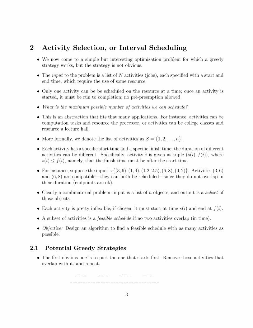
• The first obvious one is to pick the one that starts first. Remove those activities thatoverlap with it, and repeat.

---- ---- ---- ----

-----------------------------------

3

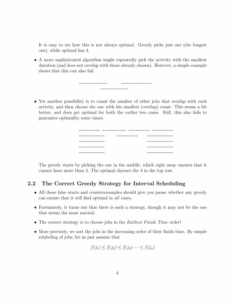
It is easy to see how this is not always optimal. Greedy picks just one (the longestone), while optimal has 4.

• A more sophisticated algorithm might repeatedly pick the activity with the smallestduration (and does not overlap with those already chosen). However, a simple exampleshows that this can also fail.

------------ -------------

------------

• Yet another possibility is to count the number of other jobs that overlap with eachactivity, and then choose the one with the smallest (overlap) count. This seems a bitbetter, and does get optimal for both the earlier two cases. Still, this also fails toguarantee optimality some times.

--------- ---------- --------- ---------

----------- --------- -----------

----------- -----------

----------- -----------

----------- -----------

The greedy starts by picking the one in the middle, which right away ensures that itcannot have more than 3. The optimal chooses the 4 in the top row.

2.2 The Correct Greedy Strategy for Interval Scheduling

• All these false starts and counterexamples should give you pause whether any greedycan ensure that it will find optimal in all cases.

• Fortunately, it turns out that there is such a strategy, though it may not be the onethat seems the most natural.

• The correct strategy is to choose jobs in the Earliest Finish Time order!

• More precisely, we sort the jobs in the increasing order of their finish time. By simplerelabeling of jobs, let us just assume that

f(j1) ≤ f(j2) ≤ f(j3) · · · ≤ f(jn)

4

• An example instance of the problem.

Activity Start Finish1 1 42 3 53 0 64 5 75 3 86 5 97 6 108 8 119 8 1210 2 1311 12 14

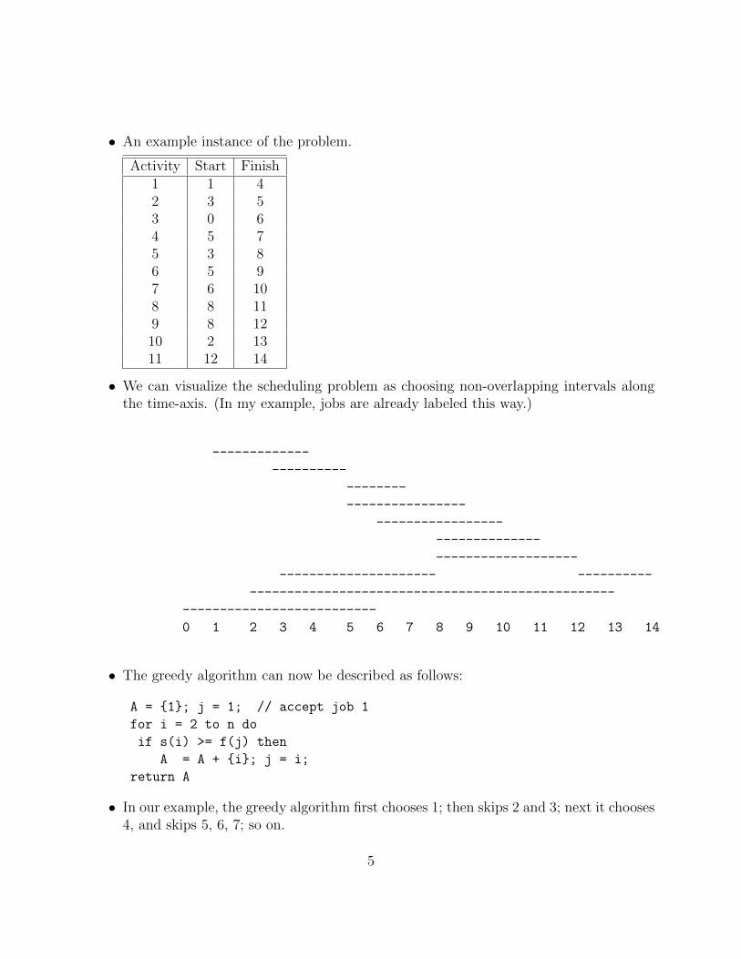
• We can visualize the scheduling problem as choosing non-overlapping intervals alongthe time-axis. (In my example, jobs are already labeled this way.)

-------------

----------

--------

----------------

-----------------

--------------

-------------------

--------------------- ----------

-------------------------------------------------

--------------------------

0 1 2 3 4 5 6 7 8 9 10 11 12 13 14

• The greedy algorithm can now be described as follows:

A = {1}; j = 1; // accept job 1

for i = 2 to n do

if s(i) >= f(j) then

A = A + {i}; j = i;

return A

• In our example, the greedy algorithm first chooses 1; then skips 2 and 3; next it chooses4, and skips 5, 6, 7; so on.

5

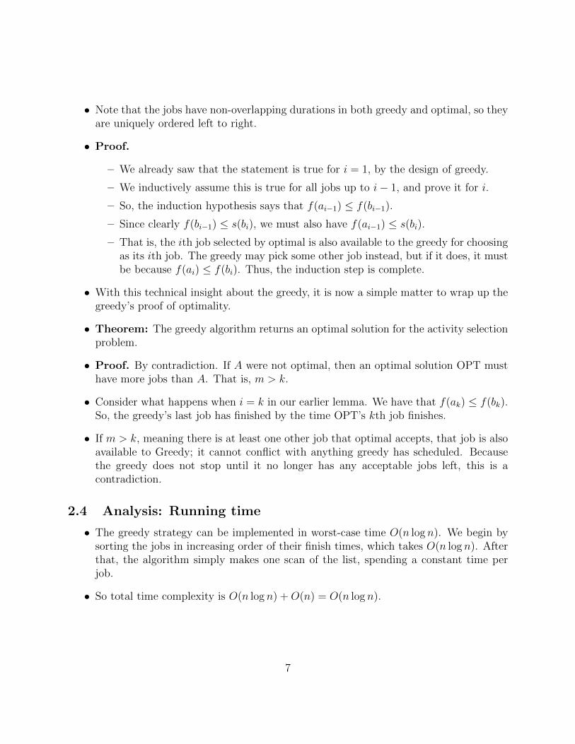
2.3 Analysis: Correctness

• It is not obvious that this method will (should) always return the optimal solution.After all, the previous 3 methods failed.

• But the method clearly finds a feasible schedule; no two activities accepted by thismethod can conflict; this is guaranteed by the if statement.

• In order to show optimality, let us argue in the following manner. Suppose OPT isan optimal schedule. Ideally we would like to show that it is always the case thatA ≡ OPT ; but this is too much to ask; in many cases there can be multiple differentoptima, and the best we can hope for is that their cardinalities are the same: that is,|A| = |OPT |; the contain the same number of activities.

• The proof idea, which is a typical one for greedy algorithms, is to show that the greedystays ahead of the optimal solution at all times. So, step by step, the greedy is doingat least as well as the optimal, so in the end, we can’t lose.

• Some formalization and notation to express the proof.

• Suppose a1, a2, . . . , ak are the (indices of the) set of jobs in the Greedy schedule, andb1, b2, . . . bm the set of jobs in an optimal schedule OPT. We would like to argue thatk = m.

• Mnemonically, ai’s are jobs picked by our algorithm while bi’s are best (optimal) sched-ule jobs.

• In both schedules the jobs are listed in increasing order (either by start or finish time;both orders are the same).

• Our intuition for greedy is that it chooses jobs in such a way as to make the resourcefree again as soon as possible. Thus, for instance, our choice of greedy ensures that

f(a1) ≤ f(b1)

(that is, a1 finishes no later than b1.)

• This is the sense in which greedy “stays ahead.” We now turn this intuition into aformal statement.

• Lemma: For any i ≤ k, we have that f(ai) ≤ f(bi).

• That is, the ith job chosen by greedy finishes no later than the ith job chosen by theoptimal.

6

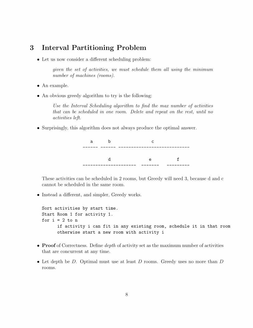
• Note that the jobs have non-overlapping durations in both greedy and optimal, so theyare uniquely ordered left to right.

• Proof.

– We already saw that the statement is true for i = 1, by the design of greedy.

– We inductively assume this is true for all jobs up to i− 1, and prove it for i.

– So, the induction hypothesis says that f(ai−1) ≤ f(bi−1).

– Since clearly f(bi−1) ≤ s(bi), we must also have f(ai−1) ≤ s(bi).

– That is, the ith job selected by optimal is also available to the greedy for choosingas its ith job. The greedy may pick some other job instead, but if it does, it mustbe because f(ai) ≤ f(bi). Thus, the induction step is complete.

• With this technical insight about the greedy, it is now a simple matter to wrap up thegreedy’s proof of optimality.

• Theorem: The greedy algorithm returns an optimal solution for the activity selectionproblem.

• Proof. By contradiction. If A were not optimal, then an optimal solution OPT musthave more jobs than A. That is, m > k.

• Consider what happens when i = k in our earlier lemma. We have that f(ak) ≤ f(bk).So, the greedy’s last job has finished by the time OPT’s kth job finishes.

• If m > k, meaning there is at least one other job that optimal accepts, that job is alsoavailable to Greedy; it cannot conflict with anything greedy has scheduled. Becausethe greedy does not stop until it no longer has any acceptable jobs left, this is acontradiction.

2.4 Analysis: Running time

• The greedy strategy can be implemented in worst-case time O(n log n). We begin bysorting the jobs in increasing order of their finish times, which takes O(n log n). Afterthat, the algorithm simply makes one scan of the list, spending a constant time perjob.

• So total time complexity is O(n log n) + O(n) = O(n log n).

7

3 Interval Partitioning Problem

• Let us now consider a different scheduling problem:

given the set of activities, we must schedule them all using the minimumnumber of machines (rooms).

• An example.

• An obvious greedy algorithm to try is the following:

Use the Interval Scheduling algorithm to find the max number of activitiesthat can be scheduled in one room. Delete and repeat on the rest, until noactivities left.

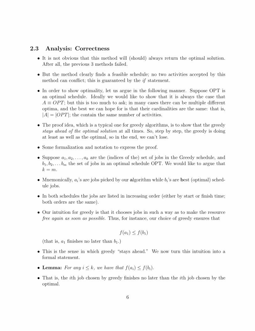
• Surprisingly, this algorithm does not always produce the optimal answer.

a b c

------ ------ ----------------------------

d e f

--------------------- ------- ---------

These activities can be scheduled in 2 rooms, but Greedy will need 3, because d and ccannot be scheduled in the same room.

• Instead a different, and simpler, Greedy works.

Sort activities by start time.

Start Room 1 for activity 1.

for i = 2 to n

if activity i can fit in any existing room, schedule it in that room

otherwise start a new room with activity i

• Proof of Correctness. Define depth of activity set as the maximum number of activitiesthat are concurrent at any time.

• Let depth be D. Optimal must use at least D rooms. Greedy uses no more than Drooms.

8

4 Data Compression: Huffman Codes

• Huffman coding is an example of a beautiful algorithm working behind the scenes, usedin digital communication and storage. It is also a fundamental result in theory of datacompression.

• For instance, mp3 audio compression scheme basically works as follows:

1. The audio signal is digitized by sampling at, say, 44KHz.

2. This produces a sequence of real numbers s1, s2, . . . , sT . For instance, a 50 minsymphony corresponds to T = 50× 60× 44000 = 130M numbers.

3. Each si is quantized, using a finite set G (e.g., 256 values for 8 bit quantization.)The quantization is fine enough that human ear doesn’t perceive the difference.

4. The quantized string of length T over alphabet G is encoded in binary.

5. This last step uses Huffman encoding.

• To get a feel for compression, let’s consider a toy example: a data file with 100, 000characters.

• Assume that the cost of storage or transmission is proportional to the number of bitsrequired. What is the best way to store or transmit this file?

• In our example file, there are only 6 different characters (G), with their frequencies asshown below.

Char a b c d e fFreq(K) 45 13 12 16 9 5

• We want to design binary codes to achieve maximum compression. Suppose we usefixed length codes. Clearly, we need 3 bits to represent six characters. One possiblesuch set of codes is:

Char a b c d e fCode 000 001 010 011 100 101

• Storing the 100K character requires 300K bits using this code. Is it possible to improveupon this?

• Huffman Codes. We can improve on this using Variable Length Codes.

9

• Motivation: use shorter codes for more frequent letters, and longer codes for infrequentletters.

• (A similar idea underlies Morse code: e = dot; t = dash; a = dot-dash ; etc. ButMorse code is a heuristics; not optimal in any formal sense.)

• One such set of codes shown below.

Char a b c d e fVLC 0 101 100 111 1101 1100

• Note that some codes are smaller (1 bit), while others are longer (4 bits) than the fixedlength code. Still, using this code2, the file requires

1× 45 + 3× 13 + 3× 12 + 3× 16 + 4× 9 + 4× 5

Kbits, which is 224 Kbits.

• Improvement is 25% over fixed length codes. In general, variable length codes can give20− 90% savings.

• Problems with Variable Length Codes. We have a potential problem with variablelength codes: while with fixed length coding, decoding is trivial, it is not the case forvariable length codes.

• Example: Suppose 0 and 000 are codes for letters x and y. What should decoder doupon receiving 00000?

• We could put special marker codes but that reduce efficiency.

• Instead we consider prefix codes: no codeword is a prefix of another codeword.

• So, 0 and 000 will not be prefix codes, but (0, 101, 100, 111, 1101, 1100), the exampleshown earlier, do form a prefix code.

• To encode, just concatenate the codes for each letter of the file; to decode, extract thefirst valid codeword, and repeat.

• Example: Code for ‘abc’ is 0101100. And ‘001011101’ uniquely decodes to ’aabe’.

10

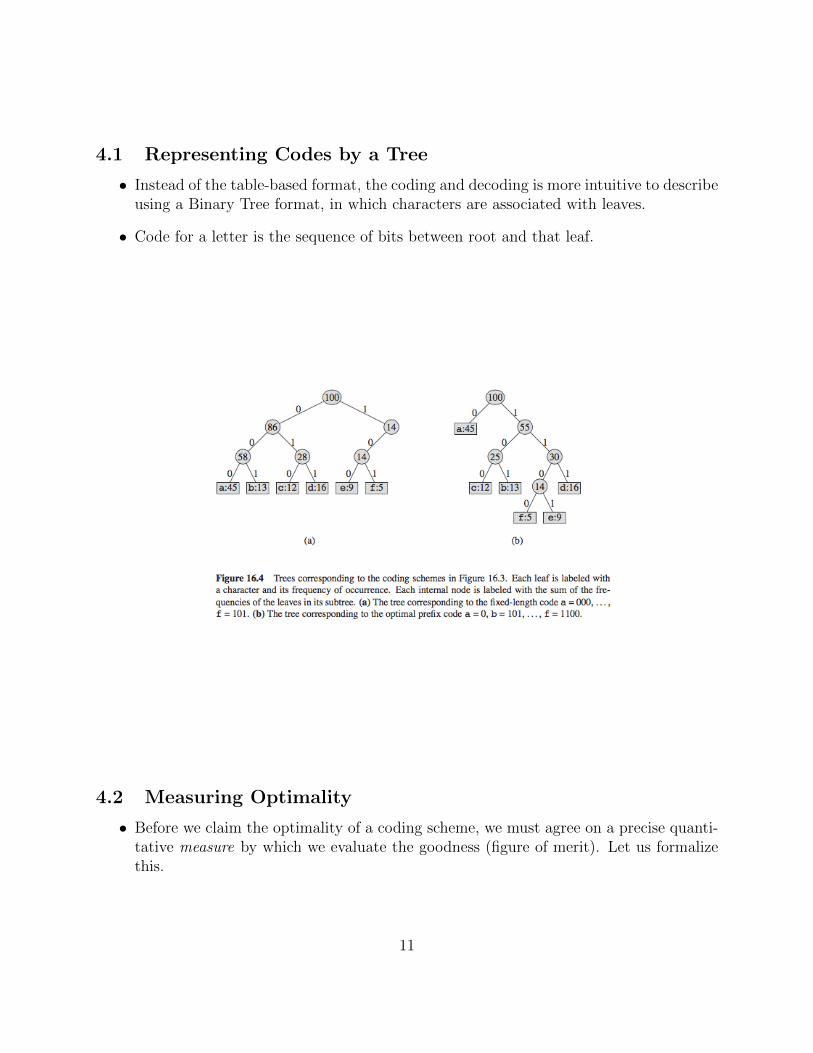
4.1 Representing Codes by a Tree

• Instead of the table-based format, the coding and decoding is more intuitive to describeusing a Binary Tree format, in which characters are associated with leaves.

• Code for a letter is the sequence of bits between root and that leaf.

4.2 Measuring Optimality

• Before we claim the optimality of a coding scheme, we must agree on a precise quanti-tative measure by which we evaluate the goodness (figure of merit). Let us formalizethis.

11

• Let C denote the alphabet. Let f(p) be the frequency of a letter p in C. Let T be thetree for a prefix code; let dT (p) be the depth of p in T . The number of bits needed toencode our file using this code is:

B(T ) =∑p∈C

f(p)dT (p)

• Think of this as bit complexity. We want a code that achieves the minimum possiblevalue of B(T ).

• Optimal Tree Property. An optimal tree must be full: each internal node has twochildren. Otherwise we can improve the code.

• Thus, by inspection, the fixed length code above is not optimal!

• Greedy Strategies. Ideas for optimal coding??? Simple obvious heuristic ideas donot work; a useful exercise will be to try to “prove” the correctness of your suggestedheuristic.

• Huffman Story: Developed his coding procedure, in a term paper he wrote whilea graduate student at MIT. Joined the faculty of MIT in 1953. In 1967, became thefounding faculty member of the Computer Science Department at UCSC. Died in 1999.

• Excerpt from an Scientific American article about this:

In 1951 David A. Huffman and his classmates in an electrical engineeringgraduate course on information theory were given the choice of a term paperor a final exam. For the term paper, students were asked to find the mostefficient method of representing numbers, letters or other symbols using abinary code. · · · Huffman worked on the problem for months, developing anumber of approaches, but none that he could prove to be the most efficient.Finally, he despaired of ever reaching a solution and decided to start studyingfor the final. Just as he was throwing his notes in the garbage, the solutioncame to him. “It was the most singular moment of my life,” Huffman says.“There was the absolute lightning of sudden realization.”

Huffman says he might never have tried his hand at the problem—much lesssolved it at the age of 25—if he had known that Fano, his professor, andClaude E. Shannon, the creator of information theory, had struggled with it.

Huffman Codes are used in nearly every application that involves the com-pression and transmission of digital data, such as fax machines, modems,computer networks, and high-definition television.

12

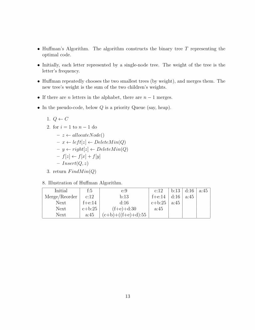
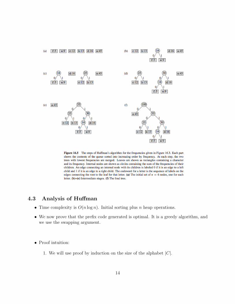
• Huffman’s Algorithm. The algorithm constructs the binary tree T representing theoptimal code.

• Initially, each letter represented by a single-node tree. The weight of the tree is theletter’s frequency.

• Huffman repeatedly chooses the two smallest trees (by weight), and merges them. Thenew tree’s weight is the sum of the two children’s weights.

• If there are n letters in the alphabet, there are n− 1 merges.

• In the pseudo-code, below Q is a priority Queue (say, heap).

1. Q← C

2. for i = 1 to n− 1 do

– z ← allocateNode()

– x← left[z]← DeleteMin(Q)

– y ← right[z]← DeleteMin(Q)

– f [z]← f [x] + f [y]

– Insert(Q, z)

3. return FindMin(Q)

8. Illustration of Huffman Algorithm.

Initial f:5 e:9 c:12 b:13 d:16 a:45Merge/Reorder c:12 b:13 f+e:14 d:16 a:45

Next f+e:14 d:16 c+b:25 a:45Next c+b:25 (f+e)+d:30 a:45Next a:45 (c+b)+((f+e)+d):55

13

4.3 Analysis of Huffman

• Time complexity is O(n log n). Initial sorting plus n heap operations.

• We now prove that the prefix code generated is optimal. It is a greedy algorithm, andwe use the swapping argument.

• Proof intuition:

1. We will use proof by induction on the size of the alphabet |C|.

14

2. The base case of |C| = 2 is trivial: we have a depth 1 tree, with two leaves, eachwith codelength 1.

3. In the general case, we will assume that induction holds for |C| = n − 1, andprove it for |C| = n.

4. Which character xi should we drop for induction? As a thought experiment,suppose we drop xn. Then, by induction, we have an optimal solution for thesubproblem on {x1, x2, . . . , xn−1}.

5. This is a tree with n− 1 leaves. How can we grow it into an n-leaf tree? We getstuck!

6. Instead, we are going to try a different idea. We take the last two charactersxn−1 and xn. We combine them into a single new character z, and set f(z) =f(xn−1) + f(xn).

7. We now remove xn−1 and xn from C and replace them with z. The new, reducedset has size |C ′| = n− 1.

8. By induction, we find the optimal code tree of C ′. This tree has z at some leaf.We now expand z by attaching the original nodes xn−1 and xn, which turns thetree for C ′ into one for C, while preserving the prefix property.

9. We are going to show that given optimal tree for C ′, this new tree will be optimalfor C.

10. This still has one problem: in our construction, the nodes xn−1 and xn will neces-sarily end up as siblings. (That is, the codes for these two will be identical exceptin the last bit.)

11. How can we choose xn−1 and xn at the onset so that in the optimal tree they areguaranteed to have this property?

12. This is where Huffman’s greedy choice enters the proof: we will choose two lowestfreq. characters.

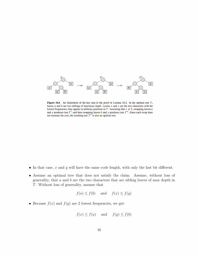
• Lemma: Suppose x and y are the two letters of lowest frequency. Then, there existsan optimal prefix code in which codewords for x and y have the same (and maximum)length and they differ only in the last bit.

• Proof. The idea of the proof is to take the tree T representing an optimal prefix code,and modify it to make a tree representing another optimal prefix code in which thecharacters x and y appear as sibling leaves of max depth.

15

• In that case, x and y will have the same code length, with only the last bit different.

• Assume an optimal tree that does not satisfy the claim. Assume, without loss ofgenerality, that a and b are the two characters that are sibling leaves of max depth inT . Without loss of generality, assume that

f(a) ≤ f(b) and f(x) ≤ f(y)

• Because f(x) and f(y) are 2 lowest frequencies, we get:

f(x) ≤ f(a) and f(y) ≤ f(b)

16

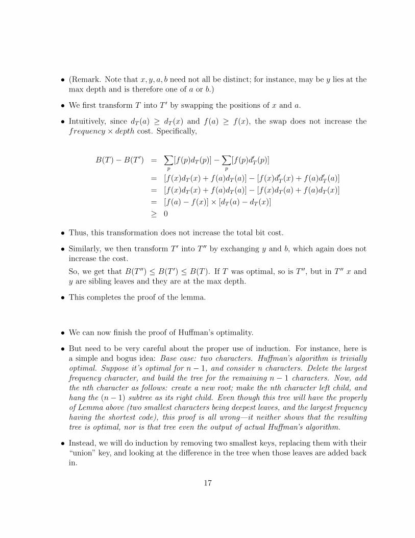
• (Remark. Note that x, y, a, b need not all be distinct; for instance, may be y lies at themax depth and is therefore one of a or b.)

• We first transform T into T ′ by swapping the positions of x and a.

• Intuitively, since dT (a) ≥ dT (x) and f(a) ≥ f(x), the swap does not increase thefrequency × depth cost. Specifically,

B(T )−B(T ′) =∑p

[f(p)dT (p)]−∑p

[f(p)d′T (p)]

= [f(x)dT (x) + f(a)dT (a)]− [f(x)d′T (x) + f(a)d′T (a)]

= [f(x)dT (x) + f(a)dT (a)]− [f(x)dT (a) + f(a)dT (x)]

= [f(a)− f(x)]× [dT (a)− dT (x)]

≥ 0

• Thus, this transformation does not increase the total bit cost.

• Similarly, we then transform T ′ into T ′′ by exchanging y and b, which again does notincrease the cost.

So, we get that B(T ′′) ≤ B(T ′) ≤ B(T ). If T was optimal, so is T ′′, but in T ′′ x andy are sibling leaves and they are at the max depth.

• This completes the proof of the lemma.

• We can now finish the proof of Huffman’s optimality.

• But need to be very careful about the proper use of induction. For instance, here isa simple and bogus idea: Base case: two characters. Huffman’s algorithm is triviallyoptimal. Suppose it’s optimal for n− 1, and consider n characters. Delete the largestfrequency character, and build the tree for the remaining n − 1 characters. Now, addthe nth character as follows: create a new root; make the nth character left child, andhang the (n− 1) subtree as its right child. Even though this tree will have the properlyof Lemma above (two smallest characters being deepest leaves, and the largest frequencyhaving the shortest code), this proof is all wrong—it neither shows that the resultingtree is optimal, nor is that tree even the output of actual Huffman’s algorithm.

• Instead, we will do induction by removing two smallest keys, replacing them with their“union” key, and looking at the difference in the tree when those leaves are added backin.

17

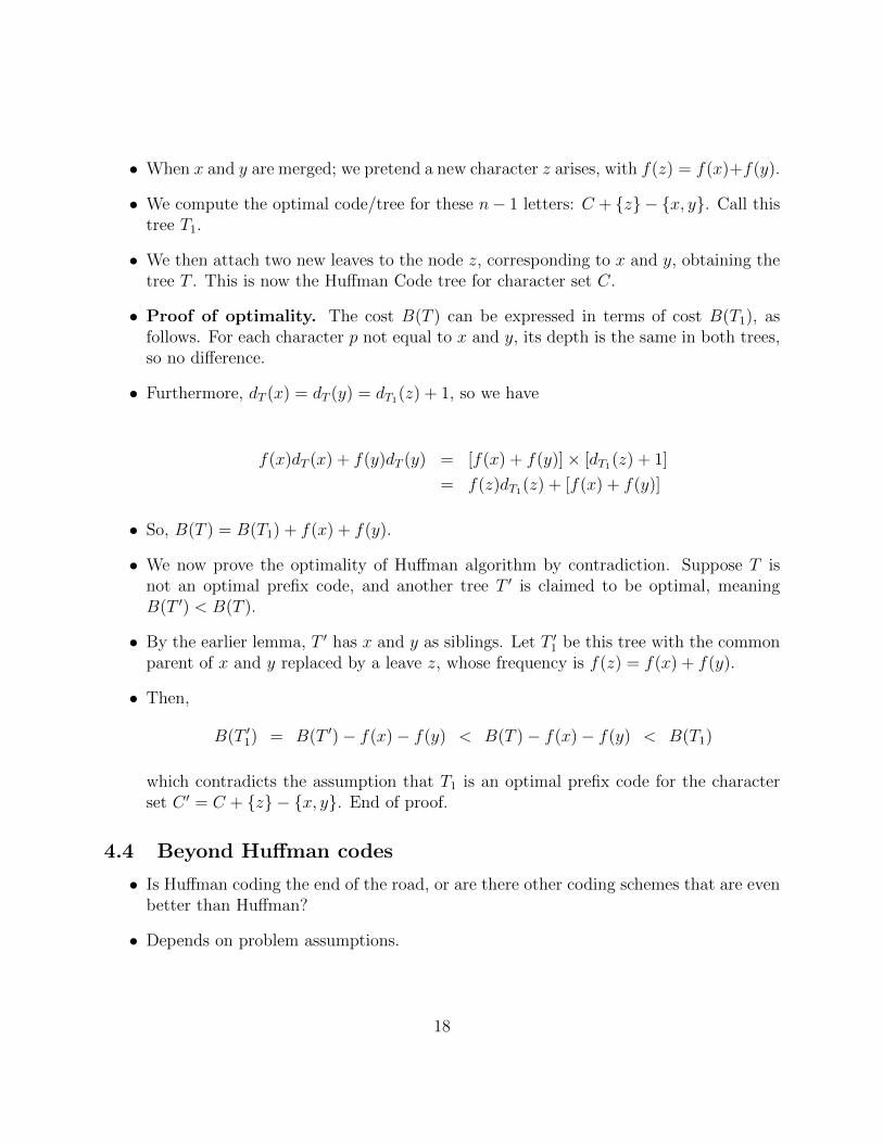
• When x and y are merged; we pretend a new character z arises, with f(z) = f(x)+f(y).

• We compute the optimal code/tree for these n− 1 letters: C + {z} − {x, y}. Call thistree T1.

• We then attach two new leaves to the node z, corresponding to x and y, obtaining thetree T . This is now the Huffman Code tree for character set C.

• Proof of optimality. The cost B(T ) can be expressed in terms of cost B(T1), asfollows. For each character p not equal to x and y, its depth is the same in both trees,so no difference.

• Furthermore, dT (x) = dT (y) = dT1(z) + 1, so we have

f(x)dT (x) + f(y)dT (y) = [f(x) + f(y)]× [dT1(z) + 1]

= f(z)dT1(z) + [f(x) + f(y)]

• So, B(T ) = B(T1) + f(x) + f(y).

• We now prove the optimality of Huffman algorithm by contradiction. Suppose T isnot an optimal prefix code, and another tree T ′ is claimed to be optimal, meaningB(T ′) < B(T ).

• By the earlier lemma, T ′ has x and y as siblings. Let T ′1 be this tree with the commonparent of x and y replaced by a leave z, whose frequency is f(z) = f(x) + f(y).

• Then,

B(T ′1) = B(T ′)− f(x)− f(y) < B(T )− f(x)− f(y) < B(T1)

which contradicts the assumption that T1 is an optimal prefix code for the characterset C ′ = C + {z} − {x, y}. End of proof.

4.4 Beyond Huffman codes

• Is Huffman coding the end of the road, or are there other coding schemes that are evenbetter than Huffman?

• Depends on problem assumptions.

18

• Huffman code does not adapt to variations in the text. For instance, if the first halfis mostly a, b, and the second half c, d, one can do better by adaptively changing theencoding.

• One can also get better-than-Huffman codes by coding longer words instead of indi-vidual characters. This is done in arithmetic coding. Huffman coding is still usefulbecause it is easier to compute (or you can rely on a table, for instance using thefrequency of characters in the English language).

• There are also codes that serve a different purpose than Huffman coding: error detect-ing and error correcting codes, for example. Such codes are very important in someareas, in particular in industrial applications.

• One can also do better by allowing lossy compression.

• Even if the goal is lossless compression, depending on the data, Huffman code mightnot be suitable: music, images, movies, and so on.

• One practical disadvantage of Huffman coding is that it requires 2 passes over the data:one to construct to code table, and second to encode, which means it can be slow andalso not suitable for streaming data. Not being error-correcting is also a weakness.

19

5 Horn Formulas

• Horn formulas are a particular form of boolean logic, and often used in AI systems forlogical reasoning.

• Each boolean variable represents an event (or possibility), such as

1. x = the murder took place in the kitchen

2. y = the butler is innocent

3. z = the colonel was asleep at 8 pm.

• A Boolean variable can only take one of two values { true, false }. A literal is either avariable x or its negation x.

• In Horn Formula, constraints among variables is represented by two kinds of clauses.

• Implication Clauses: whose left-hand-side is an AND of any number of positiveliterals, and whose right-hand-side is a single positive literal.

(z ∧ y) ⇒ x

It asserts that “if the colonel was asleep at 8 pm, and the murder took place at 8 pm,then the murder took places in the kitchen.”

A degenerate statement of the type “ ⇒ x” means that x is unconditionally true. Forinstance, “the murder definitely occurred in the kitchen.”

• Negative Clauses. Such a clause consists of an OR of any number of negative literals,as in (u ∨ t ∨ y), where u, t, y, resp., means that constable, colonel, and butler isinnocent. This clause means asserts that “they can’t all be innocent.”

• A Horn formula is a set of implications and negative clauses.

• Problem: Given a Horn formula, determine it is satisfiable. That is, is there atrue/false assignment of variables where all clauses are satisfied. Such an assignmentis called a satisfying assignment.

• Examples:

20

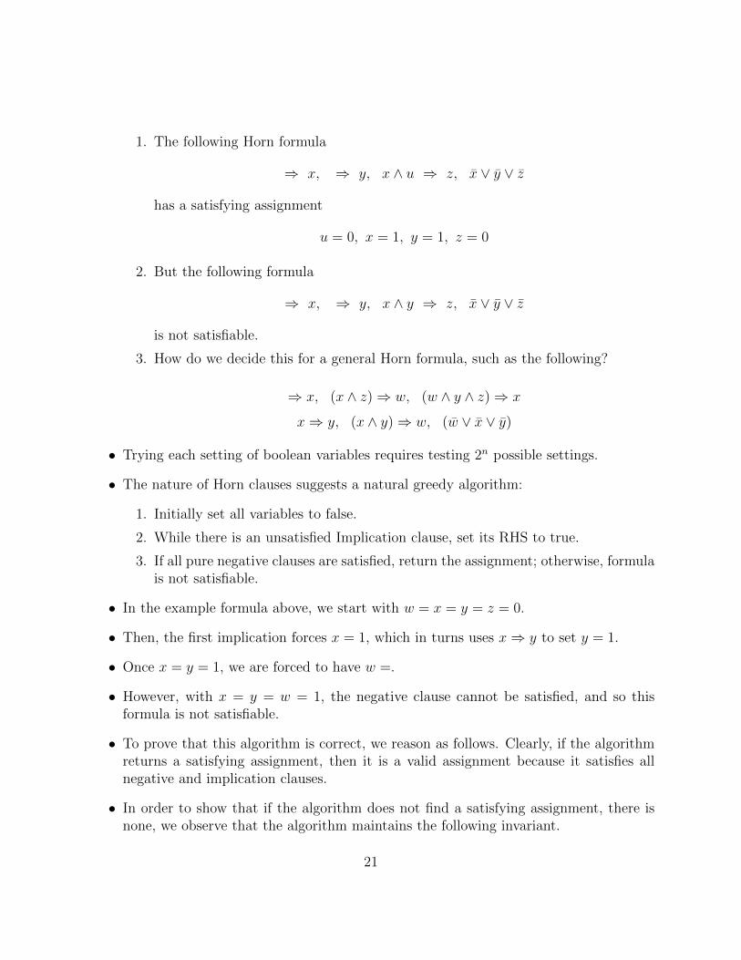
1. The following Horn formula

⇒ x, ⇒ y, x ∧ u ⇒ z, x ∨ y ∨ z

has a satisfying assignment

u = 0, x = 1, y = 1, z = 0

2. But the following formula

⇒ x, ⇒ y, x ∧ y ⇒ z, x ∨ y ∨ z

is not satisfiable.

3. How do we decide this for a general Horn formula, such as the following?

⇒ x, (x ∧ z)⇒ w, (w ∧ y ∧ z)⇒ x

x⇒ y, (x ∧ y)⇒ w, (w ∨ x ∨ y)

• Trying each setting of boolean variables requires testing 2n possible settings.

• The nature of Horn clauses suggests a natural greedy algorithm:

1. Initially set all variables to false.

2. While there is an unsatisfied Implication clause, set its RHS to true.

3. If all pure negative clauses are satisfied, return the assignment; otherwise, formulais not satisfiable.

• In the example formula above, we start with w = x = y = z = 0.

• Then, the first implication forces x = 1, which in turns uses x⇒ y to set y = 1.

• Once x = y = 1, we are forced to have w =.

• However, with x = y = w = 1, the negative clause cannot be satisfied, and so thisformula is not satisfiable.

• To prove that this algorithm is correct, we reason as follows. Clearly, if the algorithmreturns a satisfying assignment, then it is a valid assignment because it satisfies allnegative and implication clauses.

• In order to show that if the algorithm does not find a satisfying assignment, there isnone, we observe that the algorithm maintains the following invariant.

21

If a certain set of variables is set to true, then they must be true in anysatisfying assignment. Namely, we only set a variable true when it is forcedupon us.

• Horn formulas lie at the heart of Prolog programming language, and with some carethe greedy algorithm can be implemented in linear time (in the length of the formula).

22

6 Set Cover

• The set cover problem is a fundamental problem, often used to model complex decisionmaking.

• In the basic formulation, we have a base set B = {1, 2, . . . , n} of n elements, and acollection S = {S1, S2, . . . , Sm} of m subsets, with each Si ⊆ B.

• The problem is to choose the smallest number of subsets whose union is B. That is,the chosen sets jointly cover all the elements of B.

• As one example of Set Cover’s modeling power, consider the following problem. Wehave a collection of n towns in a county. The county is deciding where to put schools,subject to the following two constraints: (1) each school should be in a town, and (2)no one should have to travel more than 30 miles to reach one of the schools.

• For the purposes of modeling, we assume each town is small enough that it can berepresented as a point on the map, and so the inter-town distances are really theinter-point distances.

• For each town x, let Sx be the subset of towns within 30 miles of it. A school at x willessentially “cover” all the towns of Sx. How many sets Sx must be picked to cover allthe towns in the county?

• The problem suggests a natural greedy algorithm.Repeat until all elements of B are covered.Pick the set St containing the largest number of still-uncovered elements.

• Example from DPV book.

• The greedy algorithm will pick four sets. But there is a better solution with 3 sets.

• So, while the greedy does not give an optimal answer, its solution is not far from theoptimal.

• Claim. Suppose B contains n elements, and the optimal cover consists of k sets.Then, the greedy algorithm returns a solution with at most k lnn sets.

• Proof.

1. Let nt be the number of elements still not covered after t iterations of the greedyalgorithm. That is, n0 = n.

23

2. Since these remaining elements are covered by the optimal k sets, there must besome set that covers at least nt/k of them.

(Do we need to worry that this set may not be available any more—because greedymay have already picked it? No, because we are focusing on only those elementsthat are still uncovered—all elements of any set added to G are already in thecovered portion. Equivalently, consider the reduced problem where the base set isjust the set of remaining items, and now consider the optimal solution’s behavioron this reduced set.)

3. Since the greedy chooses a set covering most uncovered elements, we have

tt+1 ≤ nt −nt

k= nt(1−

1

k)

4. By repeated application, we get nt ≤ n0(1− 1/k)t.

5. By using the inequality 1− x ≤ e−x, for all x, we get

nt ≤ n0(1−1

k)t < n0e

−t/k = ne−t/k

6. At t = k lnn, therefore nt is strictly smaller than ne− ln = 1, which means thatno elements remain to be covered. This completes the proof.

24

7 Greedy Algorithms in Graphs

• The shortest path algorithm of Dijkstra and minimum spanning algorithms of Primand Kruskal are instances of greedy paradigm.

• We briefly review the Dijkstra and Kruskal algorithms, and sketch their proofs ofoptimality, as examples of greedy algorithm proofs.

• Dijkstra’s algorithm can be described as follows (somewhat different from the way it’simplemented, but equivalent.)

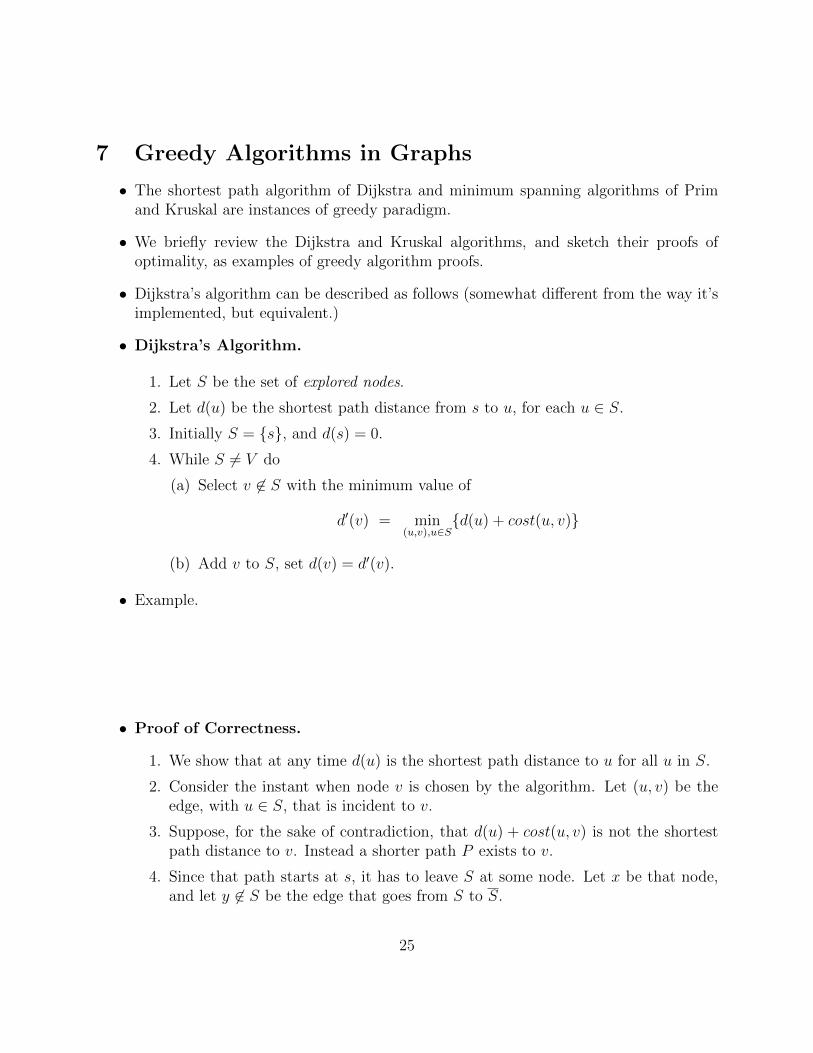
• Dijkstra’s Algorithm.

1. Let S be the set of explored nodes.

2. Let d(u) be the shortest path distance from s to u, for each u ∈ S.

3. Initially S = {s}, and d(s) = 0.

4. While S 6= V do

(a) Select v 6∈ S with the minimum value of

d′(v) = min(u,v),u∈S

{d(u) + cost(u, v)}

(b) Add v to S, set d(v) = d′(v).

• Example.

• Proof of Correctness.

1. We show that at any time d(u) is the shortest path distance to u for all u in S.

2. Consider the instant when node v is chosen by the algorithm. Let (u, v) be theedge, with u ∈ S, that is incident to v.

3. Suppose, for the sake of contradiction, that d(u) + cost(u, v) is not the shortestpath distance to v. Instead a shorter path P exists to v.

4. Since that path starts at s, it has to leave S at some node. Let x be that node,and let y 6∈ S be the edge that goes from S to S.

25

5. So our claim is that length(P ) = d(x) + cost(x, y) + length(y, v) is shorter thand(u) + cost(u, v). But note that the algorithm chose v over y, so it must be thatd(u) + cost(u, v) ≤ d(x) + cost(x, y).

6. In addition, since length(y, v) > 0, this contradicts our hypothesis that P isshorter than d(u) + cost(u, v).

7. Thus, the d(v) = d(u) + cost(u, v) is correct shortest path distance.

• Kruskal’s MST algorithm has a similar proof of correctness.

1. For simplicity, assume that all edge costs are distinct so that the MST is unique.Otherwise, add a tie-breaking rule to consistency order the edges.

2. Proof by contradiction: let (v, w) be the first edge chosen by Kruskal that is notin the optimal MST.

3. Consider the state of the Kruskal just before (v, w) is considered.

4. Let S be the set of nodes connected to v by a path in this graph. Clearly, w 6∈ S.

5. The optimal MST does not contain (v, w) but must contain a path connecting vto w, by virtue of being spanning.

6. Since v ∈ S and w 6∈ S, this path must contain at least one edge (x, y) with x ∈ Sand y 6∈ S.

7. Note that (x, y) cannot be in Kruskal’s graph at the time (v, w) was consideredbecause otherwise y will have been in S.

8. Thus, (x, y) is more expensive than (v, w) because it came after (v, w) in Kruskal’sscan order.

9. If we replace (x, y) with (v, w) in the optimal MST, it remains spanning and haslower cost, which contradicts its optimality.

10. So, the hypothesis that (v, w) is not in optimal must be false.

26