GREEK LETTERS IN RANDOM STAIRCASE TABLEAUX* SANDRINE DASSE–HARTAUT† AND PAWE L HITCZENKO‡ Abstract. In this paper we study a relatively new combinatorial object called staircase tableaux. Staircase tableaux were introduced by Corteel and Williams in the connection with Asymmetric Exclusion Process and has since found in- teresting connections with Askey–Wilson polynomials. We develop a proba- bilistic approach that allows us to analyze several parameters of a randomly chosen staircase tableau of a given size. In particular, we obtain limiting distri- butions for statistics associated with appearances of Greek letters in staircase tableaux. Key words and phrases: asymmetric exclusion process, asymptotic normality, stair- case tableaux. 1. introduction An interesting combinatorial structure, called staircase tableaux, was introduced in recent work of Corteel and Williams [9, 12]. Staircase tableaux are related to the asymmetric exclusion process on an one-dimensional lattice with open boundaries, the ASEP. This is an important and heavily studied particle model in statistical mechanics (we refer to [9] for some background information on several versions of that model and their applications and connections to other branches of science). The study of the generating function of the staircase tableau has given a combina- torial formula for the steady state probability of the ASEP. Explicit expressions for the steady state probabilities were first given in [15]. In their work [9, 12] Corteel and Williams used staircase tableaux to give a combinatorial formula for the mo- ments of the (weight function of the) Askey-Wilson polynomials; for a follow–up work see [8]. † LIAFA, Universit´ e Paris Diderot–Paris 7, F-75205 Paris, France, [email protected]. ‡ Institute of Mathematics, Polish Academy of Sciences, ul. ´ Sniadeckich 8, 00-956 Warszawa, Poland and Department of Mathematics and Information Science, Warsaw University of Technol- ogy, Pl. Politechniki 1, 00-661 Warszawa, Poland, [email protected]. * The work of the first author was carried out while she held an ANR Gamma internship at LIPN, Universit´ e Paris Nord, under the direction of Fr´ ed´ erique Bassino (LIPN) and Sylvie Corteel (LIAFA). She would like to thank both of them for their guidance, the members of LIPN for their hospitality, and ANR Gamma for the support. The second author was partially supported by NSA Grant #H98230-09-1-0062. Most of his work was done during his stay at LIPN in July 2010 and completed while he was at the Institute of Mathematics of the Polish Academy of Sciences and the Technical University of Warsaw in the Fall of 2010. He would like to thank Fr´ ed´ erique Bassino for the invitation and acknowledge the hospitality of these institutions. 1
Transcript
GREEK LETTERS IN RANDOM STAIRCASE TABLEAUX*
SANDRINE DASSE–HARTAUT† AND PAWE L HITCZENKO‡
Abstract. In this paper we study a relatively new combinatorial object calledstaircase tableaux. Staircase tableaux were introduced by Corteel and Williamsin the connection with Asymmetric Exclusion Process and has since found in-teresting connections with Askey–Wilson polynomials. We develop a proba-bilistic approach that allows us to analyze several parameters of a randomlychosen staircase tableau of a given size. In particular, we obtain limiting distri-butions for statistics associated with appearances of Greek letters in staircasetableaux.
Key words and phrases: asymmetric exclusion process, asymptotic normality, stair-case tableaux.
1. introduction
An interesting combinatorial structure, called staircase tableaux, was introducedin recent work of Corteel and Williams [9, 12]. Staircase tableaux are related to theasymmetric exclusion process on an one-dimensional lattice with open boundaries,the ASEP. This is an important and heavily studied particle model in statisticalmechanics (we refer to [9] for some background information on several versions ofthat model and their applications and connections to other branches of science).The study of the generating function of the staircase tableau has given a combina-torial formula for the steady state probability of the ASEP. Explicit expressions forthe steady state probabilities were first given in [15]. In their work [9, 12] Corteeland Williams used staircase tableaux to give a combinatorial formula for the mo-ments of the (weight function of the) Askey-Wilson polynomials; for a follow–upwork see [8].
† LIAFA, Universite Paris Diderot–Paris 7, F-75205 Paris, France, [email protected].
‡ Institute of Mathematics, Polish Academy of Sciences, ul. Sniadeckich 8, 00-956 Warszawa,Poland and Department of Mathematics and Information Science, Warsaw University of Technol-ogy, Pl. Politechniki 1, 00-661 Warszawa, Poland, [email protected].
* The work of the first author was carried out while she held an ANR Gamma internship atLIPN, Universite Paris Nord, under the direction of Frederique Bassino (LIPN) and Sylvie Corteel(LIAFA). She would like to thank both of them for their guidance, the members of LIPN for theirhospitality, and ANR Gamma for the support. The second author was partially supported byNSA Grant #H98230-09-1-0062. Most of his work was done during his stay at LIPN in July 2010and completed while he was at the Institute of Mathematics of the Polish Academy of Sciencesand the Technical University of Warsaw in the Fall of 2010. He would like to thank FrederiqueBassino for the invitation and acknowledge the hospitality of these institutions.
1
2 SANDRINE DASSE–HARTAUT AND PAWE L HITCZENKO
The authors of [9] called for further investigation of the staircase tableaux be-cause of their combinatorial interest and their potential connection to geometry.In this paper we take up that issue and study some basic properties of staircasetableaux. More precisely, we analyze the distribution of various parameters associ-ated with appearances of Greek letters α, β, δ, and γ in randomly chosen staircasetableau of size n (see the next section or, e.g. [9, Section 2], for the definitions andthe meaning of these symbols).
Staircase tableaux are generalizations of permutation tableaux (see e.g. [6, 10,11, 20] and references therein for more information on these objects and their con-nection to a version of ASEP referred to as the partially asymmetric exclusionprocess; PASEP). For permutation tableaux, the authors of [6] developed a proba-bilistic approach that later allowed the derivation of the limiting (and even exact)distributions of various parameters of the permutation tableaux. Our goal hereis the same: in Section 3 we develop a probabilistic approach parallel to that of[6] that allows us to compute generating functions of various quantities associatedwith staircase tableaux (see Corollary 6 in Section 4 and Proposition 11 in Subsec-tion 6.1.3). As a consequence, we obtain the exact or limiting distributions of theparameters we study.
Our main results are gathered in Section 5 and may be summarized by statingthat the five parameters we consider have asymptotically normal distribution whennormalized in a usual way (i.e. centered by the mean and scaled by the square rootof the variance). Thus, for example, Theorem 9 asserts that the number An of αor γ on the diagonal of a randomly chosen staircase tableau of size n has expectedvalue n/2, variance (n+1)/12 and that (An−n/2)/
√n/12 converges in distribution
to the standard normal random variable. We refer to Theorems 8 and 9 for precisestatements.
In Section 6 below (see comments at the beginning of Subsection 6.1.3 and aremark at the end of it) we find that one of the parameters we study coincideswith a generalization of Eulerian numbers (see [23, sequence A060187]) related toWhitney numbers of Dowling lattices (see [23, sequences A145901, A039775] and[16, 2, 3, 5] for definitions and further information on these numbers). This ratherunexpected and intriguing connection has not been explained and merits, perhaps,further studies. One consequence of our work is that the triangle of numbers [23,sequence A060187], when suitably normalized, satisfies the central limit theorem.As far as we can tell this result is new (although it is an easy consequence of ageneral theorem of Bender [1]). Limit theorems for a related sequence [23, A145901]are established in [5]. This link to the Whitney numbers of Dowling lattices mayhave unraveled connection to geometry alluded to in [9] as the sequences A060187,A145901, and A039775 from [23] all have a very strong geometrical flavor.
2. definitions and notation
We recall the following concept first introduced in [9, 12]: A staircase tableauof size n is a Young diagram of shape (n, n − 1, . . . , 2, 1) whose boxes are filledaccording to the following rules:
• each box is either empty or contains one of the letters α, β, δ, or γ;• no box on the diagonal is empty;• all boxes in the same row and to the left of a β or a δ are empty;• all boxes in the same column and above an α or a γ are empty.
GREEK LETTERS IN STAIRCASE TABLEAUX 3
An example of a staircase tableau is given in Figure 1(a) below.
(a) (b) (c)
Figure 1. (a) A staircase tableau of size is 7. Its top row isindexed by β, the next one by α. (b) Its type (◦ ◦ • • • ◦ ◦). (c)The same tableau with u’s and q’s.
As we mentioned, staircase (or earlier permutation) tableaux were studied inthe connection with ASEP. Because of the importance of this connection we brieflyrecall its nature. The ASEP is a Markov chain on words of size n on an alphabetA = {◦, •} consisting of two letters. Each such word represents an one-dimensionallattice of length n with some sites occupied by particles (represented by •), andothers not (represented by ◦). A particle can only hop to the right or the left(with the probabilities u and q, respectively), provided that the adjacent site isunoccupied, or enter or quit the lattice. Entering from the left (right) happenswith the probability α (resp., δ) if the first (last) site is unoccupied. Exiting to theleft (right) happens with the probability γ (resp. β) if the first (last) site is occupied.At a given time one of the n+1 possible locations for a move is selected (uniformlyat random) and, if possible, a transition described above is performed with thegiven probability. We refer to [14, 15, 17] or [9] for more detailed description andfurther references.
To describe the connection to staircase tableaux, define the type of a staircasetableau S of size n to be a word of the same size on the alphabet {◦, •} obtained byreading the diagonal boxes from northeast (NE) to southwest (SW) and writing •for each α or δ, and ◦ for each β or γ. (Thus a type of a tableau is a possible statefor the ASEP.) Figure 1(b) shows a tableau with its type. We also need a weightof a tableau S. To compute it, we first label the empty boxes of S with u’s and q’sas follows: first, we fill all the boxes to the left of a β with u’s, and all the boxes tothe left of a δ with q’s. Then, we fill the boxes above an α or a δ with u’s, and theboxes above a β or a γ with q’s. When the tableau is filled, its weight, wt(S), is amonomial of degree n(n+1)/2 in α, β, γ, δ, u and q, which is the product of labelsof the boxes of S. Figure 1(c) shows a tableau filled with u’s and q’s. Its weight isα3β2δ3γ3u8q9.
Corteel and Williams [9, 12] have shown that the steady state probability thatthe ASEP is in state σ is
Zσ(α, β, γ, δ, q, u)Zn(α, β, γ, δ, q, u)
,
where Zn(α, β, γ, δ, q, u) =∑
S of size n
wt(S) and Zσ(α, β, γ, δ, q, u) =∑
S of type σ
wt(S).
4 SANDRINE DASSE–HARTAUT AND PAWE L HITCZENKO
We denote the set of all staircase tableaux of size n by Sn, n ≥ 1. It is knownthat the cardinality of Sn is 4nn!. There are several proofs of this fact (c.f. [8] forone of them and for references to further proofs). All these proofs are based oncombinatorial approaches and we wish to mention that a probabilistic techniquethat we develop in this paper provides a yet another proof of that fact. We presentit in Section 4 below as an illustration of how our method works.
We now define some parameters that are the objects of our study. Let ∗ be asubset of the set of symbols {α, β, δ, γ}. We say that a row of a staircase tableauis indexed by ∗ if its leftmost entry is a member of ∗. For the sake of brevity wewill refer to rows indexed by ∗ simply as ∗ rows. Thus, for example, the number ofα/γ rows is the number of rows indexed by α or γ. The tableau in Figure 1(a) hastwo α/γ rows, the second from the top (indexed by α) and the bottom (indexed byγ). For a given staircase tableau S ∈ Sn we denote this quantity by rn(S) and weoccasionally skip the subscript n if there is no risk of confusion. As we demonstratein Section 3 below this parameter plays a fundamental role in our approach. Otherparameters we consider are: the total number of entries β or δ (β/δ for short), thetotal number of entries α or γ (α/γ), the number of entries β/δ on the diagonal ofthe tableau, and the number of entries α/γ on the diagonal. For a given tableauS ∈ Sn these parameters will be denoted by ∆n(S), Γn(S), Bn(S), and An(S),respectively. We gather the names and the notation we uses for the parameters weconsider along with their values for a tableau given in Figure 1(a) in the followingtable
parameter notation value in Fig. 1(a)α/γ rows rn 2
total # of β/δ ∆n 5total # of α/γ Γ 6
# of β/δ on diagonal Bn 3# of α/γ on diagonal An 4
As we mentioned earlier our viewpoint is probabilistic. Thus, we equip the setSn with the uniform probability measure denoted by Pn. This means that for eachS ∈ Sn we have
Pn(S) =1
4nn!.
As is customary we refer to a tableau chosen according to that measure as a randomtableau of size n. We denote the integration with respect to the measure Pn byEn. Our goal is to analyze probabilistic properties, like expected values, variances,and exact or limiting distributions, of random variables (or statistics) rn, ∆n, Γn,Bn, and An. We follow the probability theory conventions of [22], and the readeris pointed there for any unexplained terms.
3. Preliminaries and outline of the argument
In this section we detail main ideas beyond our approach and also derive basicproperties of the fundamental parameter, i.e. the number of α/γ rows.
Our method is analogous to what has been done in the case of permutationtableaux (see [6] or [20]). Let us recall at this point that permutation tableauxhave been used to give a combinatorial description of a stationary distribution
GREEK LETTERS IN STAIRCASE TABLEAUX 5
for the PASEP. We refer to e.g. [10, 11, 6, 20] for the definition, connections toPASEP, further properties and details. Just as PASEP is a particular case of ASEP,permutation tableaux of size n are in bijection with a subset of staircase tableauxof that size corresponding to the case γ = δ = 0.
The approach used in [6, 20] for the permutation tableaux was to identify afundamental parameter, trace its evolution as the size of a tableau is increasedby 1, and then use successively conditioning to reduce the size of a tableau. Werefer the reader to either [6] or [20] for more details, here we only recall that thisfundamental parameter was the number of unrestricted rows, Un, in a permutationtableau, and that its conditional distribution was given by 1+Bin(Un−1, 1/2) (hereBin(n, p) denotes a binomial random variable with parameters n and p). This isto mean that if a size of a permutation tableau with Un−1 unrestricted rows wasincreased from n − 1 to n, then the number of unrestricted rows in this extensionhad (the conditional) distribution 1 + Bin(Un−1, 1/2). As it turns out, in the caseof staircase tableaux the role of a fundamental parameter is played by the numberof α/γ rows.
To make our approach work we need to know two things. One is the knowledge ofthe conditional distribution of statistics of interest in extension of a given tableau ofsize n−1. This would allow us to use the so–called tower property of the conditionalexpectation to reduce the size of staircase tableaux by 1. Roughly speaking, thisreducing would amount to relating a function of a statistic on, say, Sn to anotherfunction of the same statistics on Sn−1. Keeping track of how the functions arerelated would in principle allow for an iteration of this process to reduce the sizeof the tableaux to 1. There is, however, another difficulty. Namely, when passingfrom Sn to Sn−1, not only a function of statistic changes but also a measure overwhich we integrate. More specifically, the image of the uniform probability measurePn on Sn under a natural mapping associated with our reduction does not yieldthe uniform probability measure Pn−1 on Sn−1. To handle this difficulty we need asecond ingredient which we refer to as the change of measure. It simply describes therelation between the two probability measures and allows to return to the uniformprobability measure on Sn−1 after the reduction (see Section 3.2 for more details).
In the reminder of this section we develop the details for the number of α/γ rows,a key statistic in further considerations. We do it in two separate subsections. Inthe first we analyze the evolution of the number of α/γ rows as the size of thetableaux increases. The key step is the computation of the conditional generatingfunction of rn as the size of the tableau is extended from n − 1 to n (Lemma 3below). In the second subsection we discuss the change of measure.
3.1. The conditional generating function for rn. Our analysis progresses insteps. We first find the number of extensions of a given tableau of size n − 1. Wethen find the conditional distribution of the number of α/γ rows. This enables usto compute the conditional generating function of the number of such rows in anextension of a given tableau of size n − 1. The formula expresses this generatingfunction in terms of the number of α/γ rows of the tableau being extended and isof crucial importance for our approach.
To begin the analysis we need to briefly recall the evolution process of staircasetableaux described by Corteel, Stanton, and Williams in [7]. Let S be a staircasetableau of size n− 1. To extend its size by 1, we add a new column of length n atthe left end and we fill it according to the rules. Any such filling gives a tableau
6 SANDRINE DASSE–HARTAUT AND PAWE L HITCZENKO
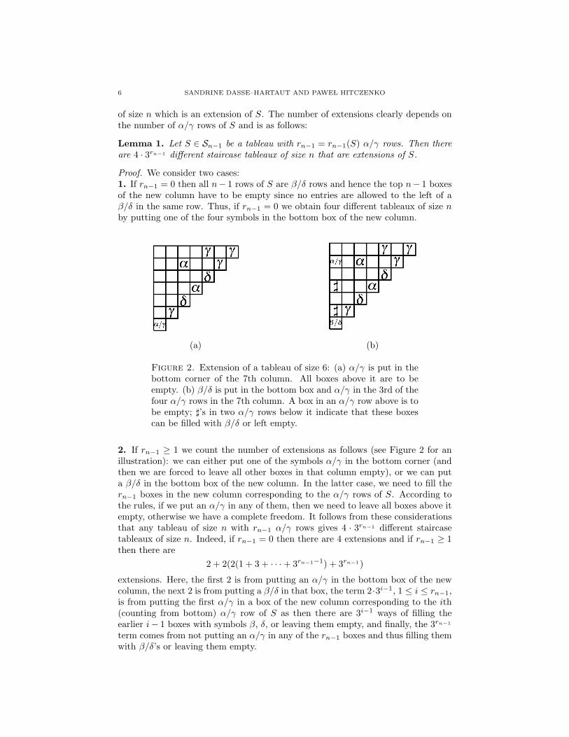
of size n which is an extension of S. The number of extensions clearly depends onthe number of α/γ rows of S and is as follows:
Lemma 1. Let S ∈ Sn−1 be a tableau with rn−1 = rn−1(S) α/γ rows. Then thereare 4 · 3rn−1 different staircase tableaux of size n that are extensions of S.
Proof. We consider two cases:1. If rn−1 = 0 then all n− 1 rows of S are β/δ rows and hence the top n− 1 boxesof the new column have to be empty since no entries are allowed to the left of aβ/δ in the same row. Thus, if rn−1 = 0 we obtain four different tableaux of size nby putting one of the four symbols in the bottom box of the new column.
(a) (b)
Figure 2. Extension of a tableau of size 6: (a) α/γ is put in thebottom corner of the 7th column. All boxes above it are to beempty. (b) β/δ is put in the bottom box and α/γ in the 3rd of thefour α/γ rows in the 7th column. A box in an α/γ row above is tobe empty; ]’s in two α/γ rows below it indicate that these boxescan be filled with β/δ or left empty.
2. If rn−1 ≥ 1 we count the number of extensions as follows (see Figure 2 for anillustration): we can either put one of the symbols α/γ in the bottom corner (andthen we are forced to leave all other boxes in that column empty), or we can puta β/δ in the bottom box of the new column. In the latter case, we need to fill thern−1 boxes in the new column corresponding to the α/γ rows of S. According tothe rules, if we put an α/γ in any of them, then we need to leave all boxes above itempty, otherwise we have a complete freedom. It follows from these considerationsthat any tableau of size n with rn−1 α/γ rows gives 4 · 3rn−1 different staircasetableaux of size n. Indeed, if rn−1 = 0 then there are 4 extensions and if rn−1 ≥ 1then there are
2 + 2(2(1 + 3 + · · ·+ 3rn−1−1) + 3rn−1)
extensions. Here, the first 2 is from putting an α/γ in the bottom box of the newcolumn, the next 2 is from putting a β/δ in that box, the term 2·3i−1, 1 ≤ i ≤ rn−1,is from putting the first α/γ in a box of the new column corresponding to the ith(counting from bottom) α/γ row of S as then there are 3i−1 ways of filling theearlier i− 1 boxes with symbols β, δ, or leaving them empty, and finally, the 3rn−1
term comes from not putting an α/γ in any of the rn−1 boxes and thus filling themwith β/δ’s or leaving them empty.
GREEK LETTERS IN STAIRCASE TABLEAUX 7
Summing the above gives
2 + 2(
23rn−1 − 1
2+ 3rn−1
)= 2 + 2(3rn−1 − 1 + 3rn−1) = 4 · 3rn−1 ,
as claimed. �
As the next step we find the conditional distribution of the number of α/γ rowsover the extensions of a given tableau of size n−1. To do that we phrase the preced-ing discussion in a more probabilistic language using what Shiryaev [22, Chapter I,§8 ] refers to as “decompositions” (which is just a special case of conditioning withrespect to σ–algebra).
Note that every tableau from Sn is an extension of a unique tableau S from Sn−1.Therefore, denoting by DS the set of all tableaux from Sn which are obtained fromS by the process described above (as we just discussed, there are 4 · 3rn−1(S) suchtableaux), we can write
Sn =⋃
S∈Sn−1
DS ,
where (DS)S∈Sn−1 are pairwise disjoint, non–empty subsets of Sn. We denote thisdecomposition of Sn by Dn−1. We wish to compute the conditional probabilitiesP( · |Dn−1) and the conditional expectations E( · |Dn−1) with respect to this de-composition. We have
Lemma 2. Let S ∈ Sn−1 be a tableau with rn−1 = rn−1(S) α/γ rows and let r bethe number of such rows in any of its extensions to a tableau of size n. Then
(1) P(r = rn−1 + 1|DS) =1
2 · 3rn−1,
and, for k = 0, 1, . . . , rn−1
(2) P(r = rn−1 − k|DS) =2k+1(2
(rn−1k+1
)+
(rn−1
k
))
4 · 3rn−1.
Proof. Let S and r be as in the statement. Clearly, the possible values for r arern−1 + 1, rn−1, rn−1 − 1, . . . , 1, 0 and we need to know the probability of each ofthese possibilities. First, r = rn−1 + 1 means that we must have placed an α/γin the bottom box of the new column since this is the only way we can increasethe number of α/γ rows. Consequently, all other boxes in the new column are toremain empty. Obviously there are two such extensions which in view of Lemma 2gives
P(r = rn−1 + 1|DS) =2
4 · 3rn−1=
12 · 3rn−1
,
which justifies (1).Next, for k = 0, 1, . . . , rn−1 we compute P(r = rn−1 − k|DS). Since k is the
number of β/δ’s that we put in the rn−1 allowable (i.e. corresponding to α/γ rowsof S) boxes, r = rn−1−k means that we put a β/δ in the bottom box and additionalk β/δ’s in the rn−1 allowable boxes above it. If we do not put an α/γ in any ofthose k boxes, we have 2 · 2k
(rn−1
k
)possibilities (2 is for putting either a β or a δ
at the bottom, and the rest accounts for putting β/δ’s in any k of the allowablern−1 boxes). If we do put an α/γ in one of the boxes we need to pick k + 1 ofthe allowable rn−1 boxes, put an α/γ in the topmost of them and put β/δ’s inthe remaining k of them (and at the bottom). This gives 2k+2
(rn−1k+1
)possibilities.
8 SANDRINE DASSE–HARTAUT AND PAWE L HITCZENKO
Adding up the two pieces and dividing by the total number of extensions given inLemma 2 we obtain,
P(r = rn−1 − k|DS) =2 · 2k
(rn−1
k
)+ 2k+2
(rn−1k+1
)4 · 3rn−1
=2k+1(2
(rn−1k+1
)+
(rn−1
k
))
4 · 3rn−1
as required. �
Lemma 2 completely describes the conditional distribution of rn given Dn−1 andleads, in particular, to the following basic relation:
Lemma 3. For a complex number z and n ≥ 1 (with the understanding that r0 ≡ 0)
(3) E(zrn |Dn−1) =z + 1
2
(z + 2
3
)rn−1
.
Proof. Recall that as we extend a tableau with rn−1 α/γ rows, we have rn = rn−1+1if and only if we put an α/γ at the bottom of the new column and rn = rn−1− k ifand only if we put a β/δ there and additional k β/δ’s in the rn−1 boxes above it.Therefore,
E(zrn |Dn−1) = E(zrnICα/γ|Dn−1) + E(zrnICβ/δ
|Dn−1)
= zrn−1+1 12 · 3rn−1
+rn−1∑k=0
zrn−1−kP(rn = rn−1 − k|Dn−1)
=z
2
(z3
)rn−1
+2
4 · 3rn−1
rn−1∑k=0
zrn−k2k
(2(rn−1
k + 1
)+
(rn−1
k
))
=z
2
(z3
)rn−1
+12
(2 + z
3
)rn−1
+1
3rn−1
rn−1−1∑k=0
zrn−k2k
(rn−1
k + 1
).
The last term is
z
2 · 3rn−1
rn−1−1∑k=0
2k+1zrn−k−1
(rn−1
k + 1
)=
z
2 · 3rn−1((2 + z)rn−1 − zrn−1) ,
so that we obtain
E(zrn |Dn−1) =z
2
(z3
)rn−1
+12
(2 + z
3
)rn−1
+z
2
(2 + z
3
)rn−1
− z
2
(z3
)rn−1
=1 + z
2
(2 + z
3
)rn−1
.
This proves (3). �
As we already mentioned, Lemma 3 (or its versions) plays a crucial role in ourapproach.
3.2. The change of measure. In this subsection we describe the second ingredi-ent, namely the change of measure. It it is necessitated by the fact that there aretwo different probability measures on Sn−1 that naturally appear in our consider-ations. The first is, of course, the uniform measure Pn−1. We discuss the secondone and the relation between them below.
Consider Sn−1, the set of all staircase tableaux of size n− 1. The second prob-ability measure on Sn−1 is obtained from the uniform probability measure on Sn
GREEK LETTERS IN STAIRCASE TABLEAUX 9
by ”collapsing” all the elements of Sn that are extensions of the same elementS ∈ Sn−1. More formally, consider a map f : Sn → Sn−1 defined by f(T ) = S ifand only if T is an extension of S. The measure of interest is the image of Pn underf . We denote this measure Pn(S) (there is an apparent ambiguity of notation here,however, it disappears once we remember whether S is in Sn or Sn−1). Since bothof these measures appear in the course of our argument, it is important to find therelationship between them. But this is straightforward: since a tableau S ∈ Sn−1
with rn−1 α/γ rows gives 4 · 3rn−1 tableaux in Sn we have
(4) Pn(S) =4 · 3rn−1
|Sn|=
4 · 3rn−1 |Sn−1||Sn|
1|Sn−1|
= 4 · 3rn−1|Sn−1||Sn|
Pn−1(S).
Consequently, for any random variable Xn−1 on Sn−1 we have
(5) EnXn−1 = En−14 · 3rn−1|Sn−1||Sn|
Xn−1 = 4|Sn−1||Sn|
En−13rn−1Xn−1.
Here we have used the same convention as above; for a random variable X on Sn−1,En−1X denotes the expectation with respect to the uniform measure on Sn−1 whileEnX denotes the expectation with respect to the measure that is induced on Sn−1
by the uniform measure on Sn.The relations (3) and (5) are key and will allow us to analyze the distributions
of the various statistics on Sn. Note that (4) and (5) are true regardless of whetherwe know the cardinalities of Sn−1 and Sn or not. As a matter of fact, one can use(5) to provide a yet another argument that |Sn| = 4nn! as we will see in the nextsection.
4. Generating function for the number of α/γ rows and someconsequences
In this section we demonstrate how we intend to apply (3) and (5) to deriverecurrences for generating functions that upon solving yield information on thecorresponding statistics. We focus here on the number of α/γ rows which, on onehand is the easiest to analyse, and on the other is central in the analysis of otherstatistics.
Proposition 4. For every complex number z we have
(6) Enzrn =
2n
|Sn|
n∏k=1
(z + 2k − 1).
Proof. By the basic properties of the conditional expectation (see e.g. [22, For-mula (16), p. 79]) the expectation on the right–hand side is equal to EnE(zrn |Dn−1).Using first (3) and then (5) we further get
Enzrn =
z + 12
En
(z + 2
3
)rn−1
=(z + 1)
24|Sn−1||Sn|
En−13rn−1
(z + 2
3
)rn−1
= 2(z + 1)|Sn−1||Sn|
En−1(z + 2)rn−1 .
Applying the same procedure with z replaced by z + 2 and n by n− 1 we obtain
Enzrn = 22(z + 1)(z + 3)
|Sn−2||Sn|
En−2(z + 4)rn−2 .
10 SANDRINE DASSE–HARTAUT AND PAWE L HITCZENKO
Further iteration yields
Enzrn = 2n−1(z + 1)(z + 3) . . . (z + 2n− 3)
|S1||Sn|
E1(z + 2(n− 1))r1 .
Since |S1| = 4 and E1(z+2(n−1))r1 = 12 (z+2(n−1))+ 1
2 the above can be writtenas
Enzrn =
2n
|Sn|(z + 1)(z + 3) . . . (z + 2n− 1),
which is precisely (6). �
Proposition 11 has a number of consequences. First, by putting z = 1 in (6)we obtain an independent confirmation of the count of staircase tableau of a givensize.
Corollary 5. Let Sn be the set of all staircase tableaux of size n ≥ 1. Then
|Sn| = 4nn!
Note that once this corollary is known (4) and (5) simplify to
(7) Pn(S) =3rn−1
nPn−1(S) and EnXn−1 =
1n
En−13rn−1Xn−1,
respectively, and this is the form we will be using from now on.Next, by combining this corollary with (6) we obtain
Corollary 6. The probability generating function of the number of α/γ rows in arandom staircase tableau of size n is given by
Enzrn =
2n
4nn!
n∏k=1
(z + 2k − 1) =n∏
k=1
z + 2k − 12k
.
The last corollary gives, in turn, a complete information on the distribution ofrn.
Corollary 7. For every n ≥ 1 we have
(8) rnd=
n∑k=1
Jk,
where Jk’s are independent and Jk is a random variable which is 1 with probability1/(2k) and 0 with the remaining probability. In particular,
(9) Enrn =n∑
k=1
12k
=Hn
2, var(rn) =
n∑k=1
12k
(1− 1
2k
)=Hn
2− H
(2)n
4,
where Hn =∑n
k=11k and H
(2)n =
∑nk=1
1k2 are harmonic numbers of the first and
second order, respectively. Furthermore,
(10)rn − ln n
2√ln n2
d−→ N(0, 1).
Proof. Note that a factorz + 2k − 1
2k=
z
2k+ 1(1− 1
2k),
GREEK LETTERS IN STAIRCASE TABLEAUX 11
given in the previous corollary is the probability generating function of a randomvariable Jk which is 1 with probability 1/(2k) and 0 with the remaining probability.Since the product of the probability generating functions corresponds to addingindependent random variables, we obtain (8) and thus also (9). Finally, sinceJk are uniformly bounded and variances of their partial sums go to infinity, theLindeberg condition for the central limit theorem (see e.g. [22, Chapter III §4])holds trivially. Since as n→∞, Enrn ∼ var(rn) ∼ ln n
2 , (10) holds. �
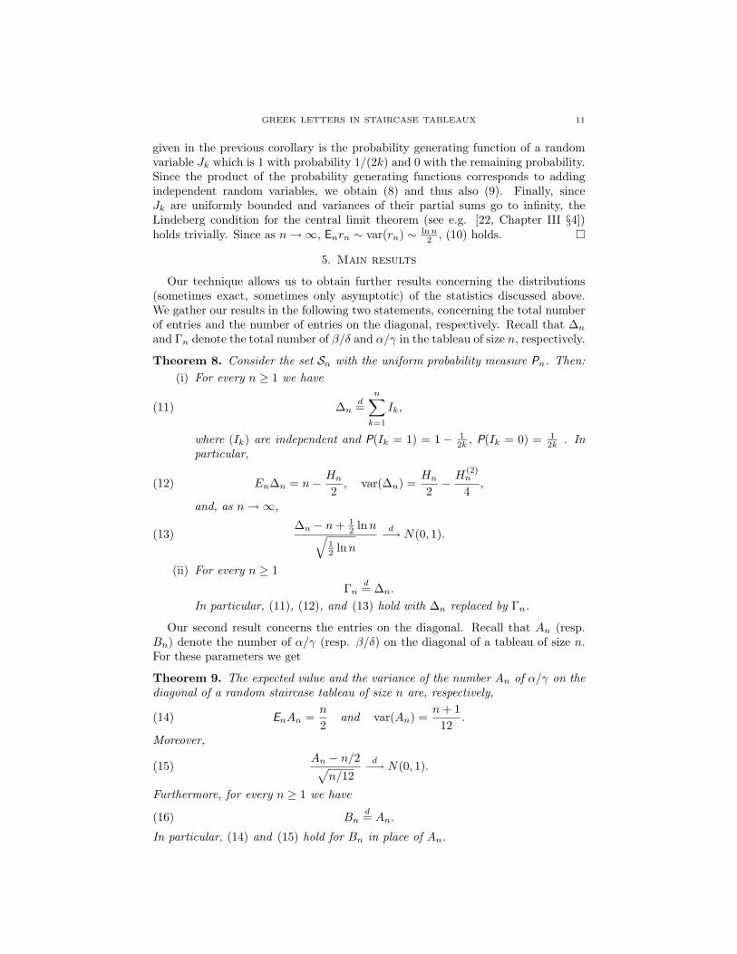
5. Main results
Our technique allows us to obtain further results concerning the distributions(sometimes exact, sometimes only asymptotic) of the statistics discussed above.We gather our results in the following two statements, concerning the total numberof entries and the number of entries on the diagonal, respectively. Recall that ∆n
and Γn denote the total number of β/δ and α/γ in the tableau of size n, respectively.
Theorem 8. Consider the set Sn with the uniform probability measure Pn. Then:(i) For every n ≥ 1 we have
(11) ∆nd=
n∑k=1
Ik,
where (Ik) are independent and P(Ik = 1) = 1 − 12k , P(Ik = 0) = 1
2k . Inparticular,
(12) En∆n = n− Hn
2, var(∆n) =
Hn
2− H
(2)n
4,
and, as n→∞,
(13)∆n − n+ 1
2 lnn√12 lnn
d−→ N(0, 1).
(ii) For every n ≥ 1Γn
d= ∆n.
In particular, (11), (12), and (13) hold with ∆n replaced by Γn.
Our second result concerns the entries on the diagonal. Recall that An (resp.Bn) denote the number of α/γ (resp. β/δ) on the diagonal of a tableau of size n.For these parameters we get
Theorem 9. The expected value and the variance of the number An of α/γ on thediagonal of a random staircase tableau of size n are, respectively,
(14) EnAn =n
2and var(An) =
n+ 112
.
Moreover,
(15)An − n/2√
n/12d−→ N(0, 1).
Furthermore, for every n ≥ 1 we have
(16) Bnd= An.
In particular, (14) and (15) hold for Bn in place of An.
12 SANDRINE DASSE–HARTAUT AND PAWE L HITCZENKO
Remark: While it seems intuitively clear that the expected number of letters α/γon the diagonal is n/2 as (14) asserts, the expression for the variance is much lessintuitive. It implies, in particular, that the entries α/γ and β/δ along the diagonalare not chosen independently from one another with equal probabilities as onemight have hoped (if that were the case the variance would be n/4).
6. proofs
We begin by observing that, as is obvious from the definition, staircase tableauxare symmetric under taking the transpose and exchanging the α’s with the β’s andthe γ’s with the δ’s. It therefore is immediate that parts (ii) of both theoremsfollow from the respective parts (i). Furthermore, the proof of Theorem 8 (i) maybe completed by using Corollary 7 and the relation
(17) rn(S) + ∆n(S) = n
since then
∆n = n− rn =n∑
k=1
(1− Jk) d=n∑
k=1
Ik.
But (17) is clear once we notice that for any row of a staircase tableau exactly oneof the following statements is true
• it contains a β/δ• it is indexed by α/γ.
This proves Theorem 8 and we now turn our attention to a considerably moreinvolved proof of Theorem 9 (i).
6.1. Proof of Theorem 9 (i). The idea is the same as for Corollary 7 except thatthis time we will actually need the joint probability generating function of An andrn. The final expression will turn out to be substantially more complicated thanwhat we encountered earlier and thus harder to analyze. Nonetheless, the situationis quite analogous to the case of the number of rows in permutation tableaux (see[20, Section 4]). For the reader’s convenience we break up our proof into severalsteps each of them discussed in a separate section below. We now briefly outlinethe major steps in the proof indicating the section in which they are treated. Webegin in the forthcoming section with the derivation of the probability generatingfunction. Its coefficients satisfy certain recurrences. This, in particular, enablesto derive the exact formulas for the expected value and the variance of An. (seeSubsection 6.1.2 below). Furthermore, the nature of these recurrences suggests thatthe coefficients are related to the classical Eulerian number associated with thenumber of rises in random permutations. In fact, our coefficients exactly much thenumbers often called the “Eulerian numbers of type B”. We establish and discussfurther this connection in Subsection 6.1.3. We think it is of independent interestand perhaps worthy of further exploration.
Once this connection is made it is then expected that the the coefficients followthe normal law (just as the classical Eulerian numbers do). As a matter of fact, oneof the proofs (although not the first) of the asymptotic normality of the classicalEulerian numbers is via a fairly general device due to Bender ([1]) and nowadaysreferred to as Bender’s theorem. This is, indeed, the approach we take and in thesubsection 6.1.4 we verify the conditions of Bender’s theorem to conclude our proof.
GREEK LETTERS IN STAIRCASE TABLEAUX 13
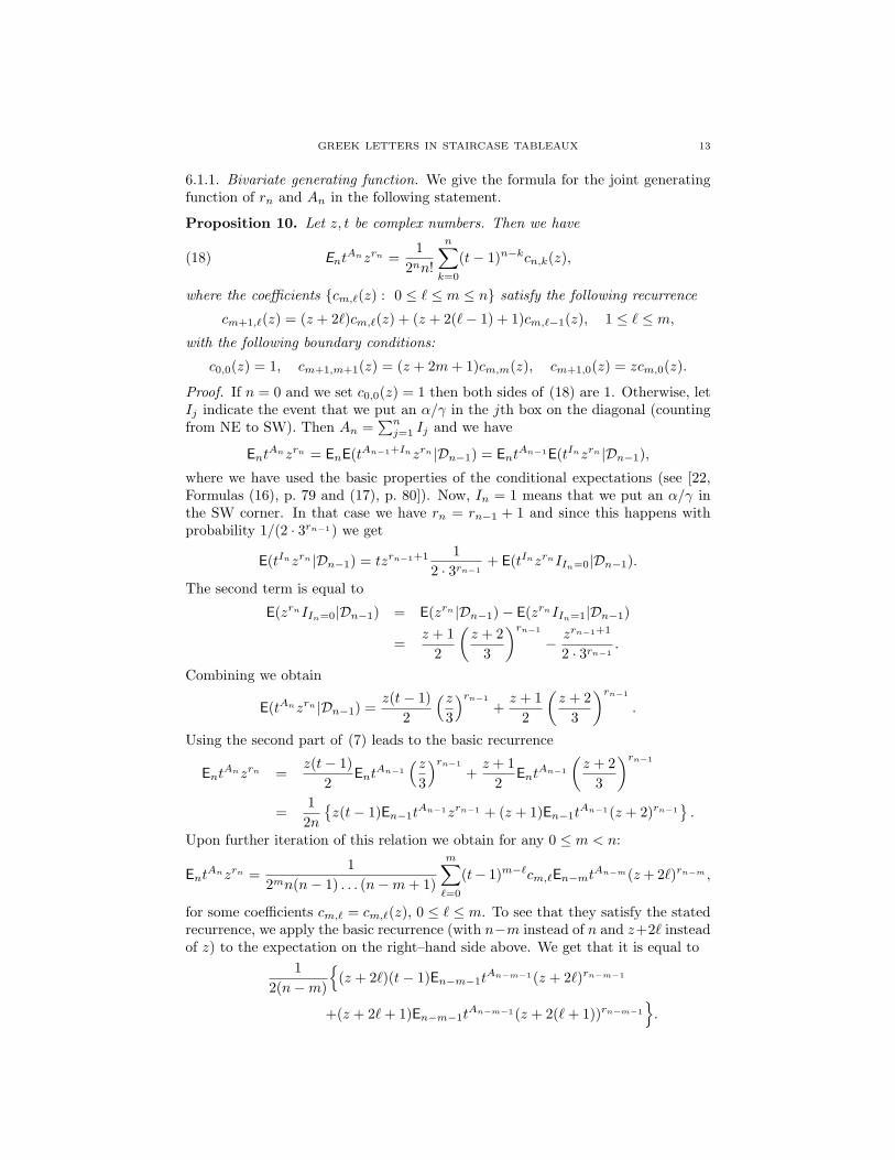
6.1.1. Bivariate generating function. We give the formula for the joint generatingfunction of rn and An in the following statement.
Proposition 10. Let z, t be complex numbers. Then we have
(18) EntAnzrn =
12nn!
n∑k=0
(t− 1)n−kcn,k(z),
where the coefficients {cm,`(z) : 0 ≤ ` ≤ m ≤ n} satisfy the following recurrence
cm+1,`(z) = (z + 2`)cm,`(z) + (z + 2(`− 1) + 1)cm,`−1(z), 1 ≤ ` ≤ m,
Proof. If n = 0 and we set c0,0(z) = 1 then both sides of (18) are 1. Otherwise, letIj indicate the event that we put an α/γ in the jth box on the diagonal (countingfrom NE to SW). Then An =
∑nj=1 Ij and we have
EntAnzrn = EnE(tAn−1+Inzrn |Dn−1) = Ent
An−1E(tInzrn |Dn−1),
where we have used the basic properties of the conditional expectations (see [22,Formulas (16), p. 79 and (17), p. 80]). Now, In = 1 means that we put an α/γ inthe SW corner. In that case we have rn = rn−1 + 1 and since this happens withprobability 1/(2 · 3rn−1) we get
E(tInzrn |Dn−1) = tzrn−1+1 12 · 3rn−1
+ E(tInzrnIIn=0|Dn−1).
The second term is equal to
E(zrnIIn=0|Dn−1) = E(zrn |Dn−1)− E(zrnIIn=1|Dn−1)
=z + 1
2
(z + 2
3
)rn−1
− zrn−1+1
2 · 3rn−1.
Combining we obtain
E(tAnzrn |Dn−1) =z(t− 1)
2
(z3
)rn−1
+z + 1
2
(z + 2
3
)rn−1
.
Using the second part of (7) leads to the basic recurrence
EntAnzrn =
z(t− 1)2
EntAn−1
(z3
)rn−1
+z + 1
2Ent
An−1
(z + 2
3
)rn−1
=12n
{z(t− 1)En−1t
An−1zrn−1 + (z + 1)En−1tAn−1(z + 2)rn−1
}.
Upon further iteration of this relation we obtain for any 0 ≤ m < n:
EntAnzrn =
12mn(n− 1) . . . (n−m+ 1)
m∑`=0
(t− 1)m−`cm,`En−mtAn−m(z+ 2`)rn−m ,
for some coefficients cm,` = cm,`(z), 0 ≤ ` ≤ m. To see that they satisfy the statedrecurrence, we apply the basic recurrence (with n−m instead of n and z+2` insteadof z) to the expectation on the right–hand side above. We get that it is equal to
12(n−m)
{(z + 2`)(t− 1)En−m−1t
An−m−1(z + 2`)rn−m−1
+(z + 2`+ 1)En−m−1tAn−m−1(z + 2(`+ 1))rn−m−1
}.
14 SANDRINE DASSE–HARTAUT AND PAWE L HITCZENKO
Substituting this into the above formula for EntAnzrn and multiplying both sides
by 2m+1n(n− 1) · · · · · (n−m) (to avoid writing a denominator on the right–handside) we get
m∑`=0
(t− 1)m−`cm,`
{(z + 2`)(t− 1)En−m−1t
An−m−1(z + 2`)rn−m−1
+(z + 2`+ 1)En−m−1tAn−m−1(z + 2(`+ 1))rn−m−1
}.
Splitting this in two sums, isolating the ` = 0 term in the first, and the ` = m inthe second, and then shifting the index in the second sum, we further obtain
cm+1,` = (z + 2`)cm,` + (z + 2(`− 1) + 1)cm,`−1, for 1 ≤ ` ≤ m.
Taking m = n− 1 we get
EntAnzrn =
12n−1n!
n−1∑`=0
(t− 1)n−1−`cn−1,`E1tA1(z + 2`)r1 ,
and since
E1tA1(z + 2`)r1 =
12t(z + 2`) +
12
=12(t− 1)(z + 2`) +
12(z + 2`+ 1),
we can write
EntAnzrn =
12nn!
n∑k=0
(t− 1)n−kcn,k,
GREEK LETTERS IN STAIRCASE TABLEAUX 15
where the coefficients {cm,` : 0 ≤ ` ≤ m ≤ n} satisfy the stated recurrence and theboundary conditions. The proof is complete. �
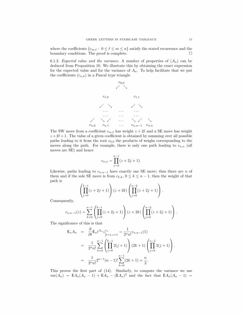
6.1.2. Expected value and the variance. A number of properties of (An) can bededuced from Proposition 10. We illustrate this by obtaining the exact expressionfor the expected value and for the variance of An. To help facilitate that we putthe coefficients (cn,k) in a Pascal type triangle.
c0,0
↙ ↘
c1,0 c1,1
↙ ↘ ↙ ↘. . . . . . . . .. . . . . . . . .
↙ ↘ ↙ . . . ↘ ↙ ↘cn,0 cn,1 . . . cn,n−1 cn,n
The SW move from a coefficient cm,` has weight z + 2` and a SE move has weightz+2`+1. The value of a given coefficient is obtained by summing over all possiblepaths leading to it from the root c0,0 the products of weighs corresponding to themoves along the path. For example, there is only one path leading to cn,n (allmoves are SE) and hence
cn,n =n−1∏j=0
(z + 2j + 1).
Likewise, paths leading to cn,n−1 have exactly one SE move; thus there are n ofthem and if the sole SE move is from ck,k, 0 ≤ k ≤ n− 1, then the weight of thatpath is k−1∏
j=0
(z + 2j + 1)
(z + 2k)
n−2∏j=k
(z + 2j + 1)
.
Consequently,
cn,n−1(z) =n−1∑k=0
k−1∏j=0
(z + 2j + 1)
(z + 2k)
n−2∏j=k
(z + 2j + 1)
.
The significance of this is that
EnAn =∂
∂tEnt
Anzrn∣∣t=1,z=1=
12nn!
cn,n−1(1)
=1
2nn!
n−1∑k=0
k−1∏j=0
2(j + 1)
(2k + 1)
n−2∏j=k
2(j + 1)
.
=1
2nn!2n−1(n− 1)!
n−1∑k=0
(2k + 1) =n
2.
This proves the first part of (14). Similarly, to compute the variance we usevar(An) = EAn(An − 1) + EAn − (EAn)2 and the fact that EAn(An − 1) =
16 SANDRINE DASSE–HARTAUT AND PAWE L HITCZENKO
∂2
∂t2 (EtAn)|t=1 = 22nn!cn,n−2(1). Paths leading to cn,n−2(1) have exactly two SE
moves, the first could be from any ck,k, 0 ≤ k ≤ n − 2 and the second from c`,`−1
for some k < ` ≤ n−1. These two moves have weights 2k+1 and 2`−1 respectively,and the remaining SW moves have weights
Thus we have proved the second part of (14) as well.
6.1.3. Connections to generalized Eulerian numbers. Before establishing the as-ymptotic normality of (An) we take a closer look at the doubly indexed sequence{cn,k} since it has intriguing connections that may be of interest in their own right.It is featured as entry A145901 in [23] and is closely related to another sequencefrom [23], namely A039755. More precisely, cn,k = 2kk!W2(n, k) where Wm(n, k)are the Whitney numbers of the second kind satisfying the recurrence
Wm(n, k) = (mk + 1)Wm(n− 1, k) +Wm(n− 1, k − 1).
The numbers (Wm(n, k)) were introduced in [16] and their properties were studiedin [2, 3, 4]. Since we are dealing exclusively with the case m = 2 we drop thesubscript and we write W (n, k) for W2(n, k). Thus, the generating function of An
may be written as
(19) ψn(t) = EntAn =
12nn!
n∑k=0
2kk!W (n, k)(t− 1)n−k.
It is perhaps of interest to mention that the numbers (2kk!W (n, k)) themselvessatisfy the central (and local) limit theorem as was shown in [5]. However, this isnot exactly what we want since the generating function above is in powers of t− 1rather than t. In terms of powers of t ψn(t) has the following form.
Proposition 11. The probability generating function of the number of α/γ entrieson the diagonal of a random staircase tableau of size n has the form
(20) ψn(t) =1
2nn!
n∑m=0
V (n,m)tm,
GREEK LETTERS IN STAIRCASE TABLEAUX 17
where the numbers {V (n,m), 0 ≤ m ≤ n} satisfy the boundary condition V (n, 0) =1, the symmetry relation V (n,m) = V (n, n−m), and the recurrence
which shows that (20) holds with V (n,m) given by (22).It remains to verify the claimed properties of the numbers V (n,m), 0 ≤ m ≤ n.
Since the symmetry condition follows by induction from the recurrence it suffices toverify the recurrence and the boundary condition. For the boundary condition, wesee immediately that for n ≥ 0 V (n, n) = W (n, 0) = 1, so that once we verify therecurrence (and thus also the symmetry) we will have that V (n, 0) = 1 for all n ≥ 0.To verify (21), we use the basic recurrence for W (n, k)’s to write the left–hand side
18 SANDRINE DASSE–HARTAUT AND PAWE L HITCZENKO
of (21) as
V (n,m) =n−m∑k=0
2kk!((2k + 1)W (n− 1, k) +W (n− 1, k − 1)
)(n− k
m
)(−1)n−m−k
=n−m∑k=0
2kk!(2k + 1)W (n− 1, k)(n− k
m
)(−1)n−m−k
+n−m∑k=1
2kk!W (n− 1, k − 1)(n− k
m
)(−1)n−m−k
=n−m∑k=0
2kk!(2k + 1)W (n− 1, k)(n− k
m
)(−1)n−m−k
+n−m−1∑
k=0
2k+1(k + 1)!W (n− 1, k)(n− k − 1
m
)(−1)n−m−k−1
= 2n−m(n−m)!(2(n−m) + 1)W (n− 1, n−m)
+n−m−1∑
k=0
2kk!(2k + 1)W (n− 1, k)(n− k
m
)(−1)n−m−k
−n−m−1∑
k=0
2kk!(2(k + 1))W (n− 1, k)(n− k − 1
m
)(−1)n−m−k.
On the other hand, the right–hand side of (21) is
(2m+ 1)n−m−1∑
k=0
2kk!W (n− 1, k)(n− 1− k
m
)(−1)n−m−k−1
+(2(n−m) + 1)n−m∑k=0
2kk!W (n− 1, k)(n− k − 1m− 1
)(−1)n−m−k
= (2m+ 1)n−m−1∑
k=0
2kk!W (n− 1, k)(n− k − 1
m
)(−1)n−m−k−1
+(2(n−m) + 1)n−m−1∑
k=0
2kk!W (n− 1, k)(n− k − 1m− 1
)(−1)n−m−k
+(2(n−m) + 1)2n−m(n−m)!W (n− 1, n−m).
So, we see that the coefficients in front ofW (n−1, n−m) in both expressions are thesame, and to complete the verification of (21) we need to see that the coefficientsare the same for the remaining values of k, 0 ≤ k ≤ n − m − 1. Cancelling thecommon factors, we need to see that
(2k + 1)(n− k
m
)− 2(k + 1)
(n− k − 1
m
)= (2(n−m) + 1)
(n− k − 1m− 1
)− (2m+ 1)
(n− k − 1
m
).
GREEK LETTERS IN STAIRCASE TABLEAUX 19
But that is straightforward: using(n−km
)=
(n−k−1
m
)+
(n−k−1m−1
)and grouping the
terms this breaks down to verifying that(n− k − 1
m
)(2k + 1− 2(k + 1) + 2m+ 1) =
(n− k − 1m− 1
)(2(n−m) + 1− 2k − 1),
or, equivalently, that
m
(n− k − 1
m
)= (n−m− k)
(n− k − 1m− 1
),
which follows immediately from the defining property of the binomial coefficients.�
Remark: Triangle of numbers V (n,m), 0 ≤ m ≤ n is featured in the OnlineEncyclopedia of Integer Sequences [23] as a sequence A060187 (with the shift inindexing: V (n,m) = T (n+ 1,m+ 1)) and is called ”Eulerian numbers of type B”.This sequence can be traced back in the literature to MacMahon’s paper [21] andit was subsequently studied in more detail in [19, Sec. 3.2] as a sequence Bn,k(1).In particular, it appears that the expression for a bivariate generating function of(V (n, k)) was derived for the first time in [19]. We use this expression in the nextsection to derive the asymptotic normality of (An).
6.1.4. Conclusion of the proof by Bender’s theorem. Using the properties of thenumbers V (n,m) given in Proposition 11 (and the identification with the sequenceA060187 from [23]) we can complete the proof of Theorem 9 by establishing (15).To do that we will rely on a general theorem due to Bender [1, Theorem 1]. (Ben-der result is also described in [18]; see Section IX.6 in general, and Theorem IX.9,Example IX.12, and Proposition IX.9 in particular). Recall from [23] or [19, For-mula (3.23)] (and see Section 3 of [19] for a proof) that the bivariate generatingfunction of the numbers (V (n, k)), called in [19] (Bn,k(1)), is∑
n≥0
n∑k=0
V (n, k)wkzn
n!=
(1− w)e(1−w)z
1− we2(1−w)z.
Therefore, it follows from (20) that the bivariate probability generating function ofthe sequence (An) is
f(z, w) :=∑n≥0
ψn(z)zn =∑n≥0
n∑k=0
V (n, k)wk
n!
(z2
)n
=(1− w)e(1−w)z/2
1− we(1−w)z,
where we define f(z, 1) = 1/(1− z). We now closely follow the way Bender appliedhis result. First,
f(z, es) =(1− es)e(1−es)z/2
1− ese(1−es)z
has a simple pole at z = r(s) = s/(es − 1). Furthermore,
with the constant in O(1) bounded when both s and z − r(s) are close to 0. Thus,by a comment at the very beginning of Section 3 of [1], the conditions of Theo-rem 1 of that paper are satisfied, and hence the central limit theorem holds (withcentering by EAn ∼ n/2 and scaling by
√var(An) ∼
√n/12 as implied by (14)).
Alternatively, we see that
r(0) = 1, r′(0) = −12, and r′′(0) =
16,
so that by [1, Theorem 1] EAn ∼ n2 and var(An) ∼ n
12 which conforms to what wehave found in (14). In any event, (15) follows.
7. Conclusion and further remarks
In this paper we have developed a probabilistic approach to the analysis ofproperties of random staircase tableaux. Using this approach we established theasymptotic normality of several parameters associated with appearances of Greekletters α, β, γ, and δ in a randomly chosen tableau. We certainly hope that thisapproach will be useful in the analysis of other properties of staircase tableaux.From the combinatorial point of view, it would be of interest to analyse the numberof appearances of the letter q in such tableaux. It is not clear at this point, thatthe method we develop is adequate to address that question, and if so, how difficultit would be to achieve. This is probably an issue worth resolving in the future.The fact that our method can be used to give new and rather complete resultsconcerning Greek letters and the fact that it gives an easy way of enumerating ofstaircase tableaux of a given size makes us cautiously optimistic.
It is perhaps worth making the following point. In our arguments we reliedon observations like (17) and symmetries of staircase tableaux to minimize theamount of work. We wish to emphasize, however, that our probabilistic approachdoes provide a unified and systematic way of analyzing each of the statistics weconsidered in a self–contained manner (i.e. not relying on relations between variousparameters). In fact, a direct proof that Γn satisfies (11), (12), and (13) was givenin [13]. This is partly a reason we believe that our approach has potential of beinguseful in addressing other questions concerning statistics of staircase tableaux. Toreiterate that point we wish to briefly sketch a proof of (16) in Theorem 9 notrelying on symmetries of the parameters.
7.1. The number of β/δ on the diagonal. We show that An and Bn haveidentical probability generating functions which, of course, implies (16). WriteBn =
∑nj=1 bj , where bj is 1 if we put a β or δ in the jth box on the diagonal
(counting SW from the top) and is 0 otherwise. We first derive the expression for
GREEK LETTERS IN STAIRCASE TABLEAUX 21
the conditional probability generating function: For z, t complex,
So, if we write bm,` = am,`t`(1 − t)m−` we see that the coefficients am,` = am,`(z)
satisfy the recurrence
am+1,` = (z + 2`)am,` + (z + 2`− 1)am,`−1,
with the initial condition
a0,0 = 1, and am,` = 0, for ` > m.
This is exactly the same recurrence as for the sequence (cn,k) defined in the lastsection and thus
(23) EntBnzrn =
12nn!
n∑k=0
cn,ktk(1− t)n−k.
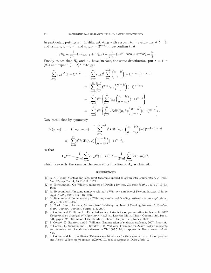
22 SANDRINE DASSE–HARTAUT AND PAWE L HITCZENKO
In particular, putting z = 1, differentiating with respect to t, evaluating at t = 1,and using cn,n = 2nn! and cn,n−1 = 2n−1n!n we confirm that
EnBn =1
2nn!(−cn,n−1 + ncn,n) =
12nn!
(−2n−1n!n+ n2nn!) =n
2.
Finally to see that Bn and An have, in fact, the same distribution, put z = 1 in(23) and expand (1− t)n−k to get
n∑k=0
cn,ktk(1− t)n−k =
n∑k=0
cn,ktk
n−k∑j=0
(n− k
j
)(−1)n−k−jtn−k−j
=n∑
k=0
n−k∑j=0
tn−jcn,k
(n− k
j
)(−1)n−k−j
=n∑
m=0
tm
{m∑
k=0
cn,k
(n− k
n−m
)(−1)m−k
}
=n∑
m=0
tm
{m∑
k=0
2kk!W (n, k)(n− k
n−m
)(−1)m−k
}.
Now recall that by symmetry
V (n,m) = V (n, n−m) =n−(n−m)∑
k=0
2kk!W (n, k)(n− k
n−m
)(−1)n−k−(n−m)
=m∑
k=0
2kk!W (n, k)(n− k
n−m
)(−1)m−k,
so that
EntBn =
12nn!
n∑k=0
cn,ktk(1− t)n−k =
12nn!
n∑m=0
V (n,m)tm,
which is exactly the same as the generating function of An as claimed.
References
[1] E. A. Bender. Central and local limit theorems applied to asymptotic enumeration. J. Com-bin. Theory Ser. A, 15:91–111, 1973.
[2] M. Benoumhani. On Whitney numbers of Dowling lattices. Discrete Math., 159(1-3):13–33,1996.
[3] M. Benoumhani. On some numbers related to Whitney numbers of Dowling lattices. Adv. inAppl. Math., 19(1):106–116, 1997.
[4] M. Benoumhani. Log-concavity of Whitney numbers of Dowling lattices. Adv. in Appl. Math.,22(2):186–189, 1999.
[5] L. Clark. Limit theorems for associated Whitney numbers of Dowling lattices. J. Combin.Math. Combin. Comput., 50:105–113, 2004.
[6] S. Corteel and P. Hitczenko. Expected values of statistics on permutation tableaux. In 2007Conference on Analysis of Algorithms, AofA 07, Discrete Math. Theor. Comput. Sci. Proc.,AH, pages 325–339. Assoc. Discrete Math. Theor. Comput. Sci., Nancy, 2007.
[7] S. Corteel, D. Stanton, and L. Williams. Enumeration of staircase tableaux, 2007. Preprint.[8] S. Corteel, D. Stanton, and R. Stanley L. K. Williams. Formulae for Askey–Wilson moments
and enumeration of staircase tableaux. arXiv:1007.5174, to appear in Trans. Amer. Math.Soc.
[9] S. Corteel and L. K. Williams. Tableaux combinatorics for the asymmetric exclusion processand Askey–Wilson polynomials. arXiv:0910.1858, to appear in Duke Math. J.
GREEK LETTERS IN STAIRCASE TABLEAUX 23
[10] S. Corteel and L. K. Williams. A Markov chain on permutations which projects to the PASEP.Int. Math. Res. Notes, 17, 2007. Art. ID rnm055, 27pp.
[11] S. Corteel and L. K. Williams. Tableaux combinatorics for the asymmetric exclusion process.Adv. Appl. Math,, 39:293–310, 2007.
[12] S. Corteel and L. K. Williams. Staircase tableaux, the asymmetric exclusion process, andAskey- Wilson polynomials. Proc. Natl. Acad. Sci, 107(15):6726–6730, 2010.
[13] S. Dasse-Hartaut and P. Hitczenko. Some properties of random staircasetableaux. Proceedings of the ANALCO 2011 meeting, pp. 58-66, SIAM 2011.http://www.siam.org/proceedings/analco/2011/analco11.php.
[14] B. Derrida, E. Domany, and D. Mukamel. An exact solution of a one dimensional asymmetricexclusion process with open boundaries. J. Statist. Phys., 69(3-4):667–687, 1992.
[15] B. Derrida, M. R. Evans, V. Hakim, and V. Pasquier. Exact solution of a 1D asymmetricexclusion model using a matrix formulation. J. Phys. A, 26(7):1493–1517, 1993.
[16] T. A. Dowling. A class of geometric lattices based on finite groups. J. Combinatorial TheorySer. B, 14:61–86, 1973. (Erratum: J. Combinatorial Theory Ser. B, 15:211, 1973).
[17] E. Duchi and G. Schaeffer. A combinatorial approach to jumping particles. J. Combin. TheorySer. A, 110(1):1–29, 2005.
[18] P. Flajolet and R. Sedgewick. Analytic combinatorics. Cambridge University Press, 2009.[19] G. R. Franssens. On a number pyramid related to the binomial, Deleham, Eulerian, MacMa-
hon and Stirling number triangles. J. Integer Seq., 9(4):Article 06.4.1, 34 pp. (electronic),2006.
[20] P. Hitczenko and S. Janson. Asymptotic normality of statistics on permutation tableaux.Contemporary Math., 520:83–104, 2010.
[21] P.A. MacMahon. The divisors of numbers. Proc. London Math. Soc., 19:305–340, 1920.[22] A. N. Shiryaev. Probability, volume 95 of Graduate Texts in Mathematics. Springer-Verlag,
New York, second edition, 1996.[23] N. J. A. Sloane. The On-Line Encyclopedia of Integer Sequences, 2006.