Green productivity in agriculture - OECD.org 4 Timo Kuosmanen Green_agricultur… · 4.2 Generic...

Green productivity in agriculture:A critical synthesis

Timo Kuosmanen1,2

1) Professor, Aalto University School of Business, Helsinki, Finland.2) Associate, Sigma-Hat Economics Oy.

E-mail: [email protected].

Green productivity in agriculture: a critical synthesis

2

TABLE OF CONTENTS

Tables 2Figures 2Excecutive summary 4List of acronyms 51. Introduction 62. Productivity indices 83. Environmental productivity and efficiency 114. Estimation of technology distance functions 14

4.1 Brief literature review 144.2 Generic econometric model 15

5. Model specification and some methodological issues specific to agriculture 165.1 Damage control inputs 165.2 Material balance 165.3 Production risk 185.4 Critical synthesis 19

6. Environmental issues specific to agriculture 197. Empirical application 20

7.1 Data and model specification 207.2 Stochastic semi-nonparametric envelopment of data 237.3 Parametric SFA 287.4 Stochastic DEA 327.5 Evolution of country specific TFP measures over time 34

8. Concluding remarks and recommendations 35References 38Appendix 1: Main features and assumptions of the different econometric methods applied in thisstudy 45Appendix 2: Evolution of ECON, ENV, and MIX measures of TFP at the country level 47

TABLES

Table 1: Labour productivity (y/L) in the sample countries; averages of 1990 – 2004 22Table 2: Capital productivity (y/K) in the sample countries; average of 1990 – 2004 23Table 3: Marginal products of inputs in ECON, ENV, and MIX models: summary statistics of the CNLSestimates (prices of 2004 – 2006) 24Table 4: Parameter estimates of the time trend; semi-nonparametric StoNED model 25Table 5: Efficiency levels, efficiency change, and TFP change according to the ECON model; Semi-nonparametric StoNED estimates 26Table 6: Efficiency levels, efficiency change, and TFP change according to the ENV model; Semi-nonparametric StoNED estimates 27Table 7: Efficiency levels, efficiency change, and TFP change according to the MIX model; Semi-nonparametric StoNED estimates 27Table 8: The results of the ECON, ENV, and MIX models estimated by OLS 29Table 9: Efficiency levels, efficiency change, and TFP change according to the ECON model; Cobb-Douglas production function estimated by OLS 30Table 10: Efficiency levels, efficiency change, and TFP change according to the ENV model; Cobb-Douglas production function estimated by OLS 30Table 11: Efficiency levels, efficiency change, and TFP change according to the MIX model; Cobb-Douglas production function estimated by OLS 31


3

Table 12: Efficiency levels and TFP change according to the ECON model; inter-temporal productionfunction estimated by stochastic DEA 32Table 13: Efficiency levels and TFP change according to the ENV model; inter-temporal productionfunction estimated by stochastic DEA 33Table 14: Efficiency levels and TFP change according to the MIX model; inter-temporal productionfunction estimated by stochastic DEA 34Table A1: Classification of frontier models 45


4

Executive summary

This report has been prepared for the OECD with a view towards the development of the green growthstrategy for the agricultural sector. The purposes of this study are three-fold.

1) Review the literature for available approaches for measuring green productivity in agriculture, andprovide a critical synthesis.2) Propose an operational method for assessing green productivity in agriculture at cross-country level.3) Illustrate the proposed method and the information it can provide with an empirical study.

Since the empirical literature on agricultural productivity is large, the literature review presented in thisreport aims to structure the literature by pointing out some relevant streams together with some keyreferences. Our review starts with the discussion of alternative approaches to constructing total factorproductivity (TFP) indices, keeping in mind the environmental effects that do not typically have observablemarket prices. Therefore, we pay particular attention to the frontier approaches to TFP measurement,where the aggregation of inputs and outputs is conducted by applying shadow prices rather than marketprices. We briefly review parametric, nonparametric, and semi-nonparametric approaches asmethodological alternatives to frontier estimation. We then discuss specific methodological issues relatedto agriculture. These include the modelling of damage control inputs, the material balance accounting andits interpretation, and the modelling of production risk. We then turn attention to environmental issuesspecific to agriculture, recognizing the nutrient emissions and the green-house gas emissions as potentialindicators for which comparable data are available.

In the empirical part of the paper, we examine a panel of 13 OECD countries over the time period 1990 –2004. The countries, time horizon, and the environmental variables have been chosen based on dataavailability. We use the net production value obtained from the FAOSTAT as the output variable. As forthe input variables, we compare three alternative model specifications:i) The economic model (ECON) that includes the conventional production factors: labour, capital stock,and the land area.ii) The environmental model (ENV) that includes the agricultural green-house gas emissions, the nitrogenstock, the phosphorus stock, and the land area as the environmental resources.iii) The mixed model (MIX) that includes all input variables of both the ECON and ENV models describedabove.

These three models are estimated using three alternative econometric methods:a) Stochastic Frontier Analysis (SFA), which is a stochastic, parametric approach to frontier estimation,widely used in the applied econometrics literature.b) Data Envelopment Analysis (DEA), which is a deterministic, nonparametric approach, used in particularin the operational research literature.c) Stochastic semi-Nonparametric Envelopment of Data (StoNED), which is a recently developed approachthat combines the DEA-style nonparametric frontier with a SFA-style probabilistic treatment ofinefficiency and noise.

The empirical application indicates large differences across countries in both the level of TFP and itsgrowth rate. Further, the results differ considerably depending on the specification of the set of inputvariables and the choice of the estimation method.

Interestingly, the ENV model yields a better empirical fit than the ECON model: the environmentalindicators explain a larger proportion of variance in the net production value than the conventional primaryinputs. As a result, the results of the ENV and MIX models are more similar to each other, while the resultsof the ECON model deviate considerably from the other two model specifications.


5

The results also depend on the choice of the frontier estimation method. The results of the SFA andStoNED methods are relatively similar, particularly in the ENV and MIX models. The DEA results differnotably from those obtained with the other two methods. These findings suggest that the results arerelatively robust to the assumptions regarding the functional form of the frontier, and that explicitmodelling of stochastic noise is a more critical factor in this application.


6

List of acronyms

CO2 - Carbon Dioxide

CRS - Constant returns to scale

DEA - Data Envelopment Analysis

DI - Input distance function

ECON - Model specification where only economic production factors are used asinputs.

EE - Environmental efficiency (index)

EFF - ‘Efficiency change’: the sub-component of the Malmquist TFP index thatrepresents the movement of the country towards the frontier (catching up) oraway from the frontier (falling behind)

ENV - Model specification where only environmental indicators are used as inputs.

EU - The European Union

FAOSTAT - Statistical database of the Food and Agriculture Organization of theUnited Nations

GHG - Green-House Gas

LA - Land area: the total utilized agricultural area (in ha)

MIX - Model specification that includes both economic and environmental inputs.

ML - Maximum likelihood

OECD - Organization for Economic Cooperation and Development

OLS - Ordinary Least Squares

SFA - Stochastic Frontier Analysis

StoNED - Stochastic semi-Nonparametric Envelopment of Data

TECH - ‘Technical change’: the sub-component of the Malmquist TFP index thatrepresents the shift of the frontier over time

TFP - Total Factor Productivity

UNFCCC - United Nations Framework Convention on Climate Change

VA - Value added


7

1. Introduction

OECD has developed a Green Growth Strategy since 2009, together with partners across government andcivil society. The purpose of this strategy is to help countries achieve economic growth and developmentwhile at the same time combating climate change and preventing costly environmental degradation and theinefficient use of natural resources. The first proposal of green growth indicators was published in thereport OECD (2011a), where production is taken as the starting point, and thus the proposed indicators canbe viewed as measures of environmental or resource productivity. The strategy for green growth in foodand agriculture is outlined in OECD (2011b), based on studies by Asche (2011), Blandford (2011), Burrell(2011), Hall and Dorai (2010), and Stevens (2011).

Agriculture is one of the key sectors for green growth. Agriculture causes or contributes to several of themost serious global environmental problems, such as deforestation, water stress, eutrophication of surfaceand underground water systems, discharge of toxic waste from pesticides, and green-house gas (GHG)emissions (e.g. methane from manure). Accounting for the environmental externalities in the agriculturalproductivity analysis presents major challenges, both methodologically and empirically.

The objectives of this study are threefold. Our first objective is to survey the available approaches formeasuring green productivity in agriculture, and provide a critical synthesis. Based on the critical survey,our second objective is to propose a systematic method for assessing green productivity in agriculture atcross-country level. Thirdly, we illustrate the proposed method and the information it can provide with anempirical study to 13 countries in years 1990 – 2004, using three environmental variables: GHG emissionsfrom agriculture, and the stocks of nitrogen and phosphorus accumulated in agricultural land. Thecountries, time horizon, and the environmental variables have been chosen based on data availability.While the empirical application is limited in terms of the number of countries, years, and environmentalvariables, we believe the empirical comparisons presented below will provide useful methodologicalinsights.

Regarding the literature review, we must emphasize that the literature related to this theme is very largeand scattered over several disciplines such as agricultural economics, agronomy, ecological andenvironmental economics, econometrics, production economics, and operations research, among others.The empirical literature can be classified according to the scope as farm and sector level studies (e.g.,Reinhard et al., 1999, 2000; Brümmer et al., 2002), aggregate level country specific studies (e.g., the USAin Cox and Chavas, 1990, Jorgenson and Gollop, 1992, Ball, Hallahan, and Nehring, 2004; the UK inThirtle and Bottomley, 1992; China in Kalirajan et al., 1996; Fan and Zhang, 2002), and international crosscountry comparisons (e.g., Bureau et al., 1995; Lusigi and Thirtle, 1997; Ball et al., 2001; Coelli andPrasada Rao, 2005). The common methodological approaches in this literature include the growthaccounting (e.g., Jorgenson and Gollop, 1992), index number approaches (e.g., Kuosmanen et al., 2004;Kuosmanen and Sipiläinen, 2009; O’Donnell, 2010), and frontier approaches such as the data envelopmentanalysis (DEA) (e.g., Bureau et al., 1995) and stochastic frontier analysis (SFA) (e.g., Coelli and PrasadaRao, 2005). Recently, many empirical TFP studies in the agricultural sector try to take at least someenvironmental considerations into account (e.g., Reinhard et al., 1999, 2000; Reinhard and Thijssen, 2000;Ball, Lovell, Nehring, and Luu, 2004; Coelli et al., 2007). Given a large amount of literature, our objectiveis not to identify and cite every study that is relevant in this theme, but rather, try to provide some structureto the enormous literature, and pinpoint some important streams of literature that deserve to be considered.

The rest of the report is organized as follows. Section 2 introduces some standard approaches toproductivity measures and discusses the choice of the appropriate index number in the present context.Section 3 examines how environmental indicators could be incorporated to productivity and efficiencyanalysis. Section 4 discusses some alternative approaches to the estimation of technology distance


8

functions, which can provide shadow prices for the environmental factors and other inputs and outputs thatare not traded in competitive markets. Section 5 reviews some issues related to the econometric modelspecification, which are relevant in the context of agriculture. Section 6 discusses environmental issuesrelated to agriculture, and introduces the three environmental factors considered in the empiricalapplication. Section 7 presents an empirical analysis of 13 OECD countries in years 1990 – 2004. Theempirical comparison considers three alternative orientations to productivity measurement as well as threealternative frontier estimation techniques. Finally, Section 8 provides concluding remarks and themethodological recommendations.

2. Productivity indices

Productivity is generally understood as the ratio of output to input (e.g., OECD, 2001). In the case of asingle input x and a single good output y, the level of productivity is simply

Prod = yx

.

The productivity change from period t to t+1 is measured by the index1 1/Prod = 100

/

t t

t t

y xy x

.

The distinction between the level and the change of productivity is worth emphasizing, as the two get oftenconfused in casual conversation. When economists talk about productivity, they usually refer to theproductivity indices that measure the productivity change. However, the level of productivity is also ofinterest in the present context. The term catching up refers to the fact that countries with low level ofproductivity initially can exhibit much high productivity growth rates than countries that have alreadyachieved a high level of productivity (see, e.g., Ball, Hallahan, and Nehring, 2004, for further discussion).

The main difficulty in productivity measurement concerns the aggregation of multiple inputs and multipleoutputs to input and output indices. Agriculture is a prime example of a sector where joint production ofmultiple outputs using multiple resources is common. Agricultural production process can be modelled astransformation of multiple inputs denoted by vector x (e.g., land, capital, labour, feed, fertilizers, etc.) tomultiple outputs denoted by vector y (e.g., crops, milk, meat, eggs, vegetables etc.). The input vector xmay contain both economic inputs such as labour and capital, and environmental or natural resources suchas GHG emissions or energy consumption. Without a loss of generality, we can partition the input vectoras ( , )ECON ENVx x x , where ECONx is the vector of economic resources and ENVx is the vector ofenvironmental resources. In a similar fashion, the output vector y contains economic outputs (goods andservices) as well as environmental services (e.g., landscape management). In this report we assume alloutputs y are desirable (i.e., goods), and the use of all inputs is costly.

At the aggregate level, it is not always obvious whether an environmental indicator should be treated as aninput or an output. For example, GHG emissions are obviously an output from the perspective ofproduction, but from the perspective of the society, the GHG emissions can be seen as a burden to thenature’s absorptive capacity, which is an input. By this argument, the conventional approach in theenvironmental economics literature is to model undesirable outputs as inputs (e.g., Cropper and Oates,1992; Hailu and Veeman, 2001). Recently, the appropriate modelling of environmental bads as inputs oroutputs has attracted critical debate (see, e.g., Färe and Grosskopf, 2003; Kuosmanen and Podinovski,2009, for discussion and further references). One important study worth noting is Korhonen and Luptacik(2004), where it is shown that in the DEA method the specification of environmental factors (e.g., theGHG emissions) as inputs or outputs does not affect the efficient frontier. However, the specification canaffect the scaling properties of the technology (e.g., the returns to scale, scale elasticity and scale


9

efficiency) and the measurement of efficiency as a distance to the frontier. At the aggregate level, however,it is usual to assume the benchmark technology exhibits constant returns to scale (CRS) (see, e.g., Färe etal., 1994; or Kuosmanen and Sipiläinen, 2009). For convenience, in this report we assign all undesirablefactors (whether inputs or outputs to production) to vector x, and we attribute all desirable factors (whetherinputs or outputs) to vector y.

Introduction of environmental factors to vectors x and y increases the dimensionality of these vectors, butthe fundamental challenge remains: to measure productivity, we need to aggregate the elements of x and y,in one way or another, to obtain an input quantity index and an output quantity index. There are severalways to approach this challenge.

Partial productivity measures consider the ratio of a single output (or some aggregate measure such as therevenue) to a chosen input of interest. For example, labour productivity could be measured in physicalunits as crop yield per hour of labour, or in monetary terms as agricultural revenue per wage expenses. In asimilar vein, the commonly used eco-efficiency indicators are typically constructed as a ratio of goodoutput to bad output (y/b), where the nominator and the denominator are chosen arbitrarily from theelements of vectors y and b, or using some aggregated quantity (e.g., the average of the elements of vectorb subject to some kind of prior normalization). While the partial productivity and eco-efficiency rationscan be simple and intuitive, their interpretation can be difficult as it is often unclear what the optimal orappropriate level of labour productivity (or eco-efficiency) should be. The optimal level would likelydepend on a number of factors such as the relative prices of other resources such as land and capital.Maximizing labour productivity or eco-efficiency is not the (usual) objective of the firm. While partialproductivity indices can be useful proxy indicators in some context, the exact information content of thesesimple indicators is questionable. Further, trying to compare multiple partial productivity indicators canconfuse the overall picture, and even lead to a misleading assessment of the overall productivityperformance.

The measurement of total factor productivity (TFP) requires a more systematic aggregation of inputs andoutputs to an input index and an output index (respectively), in one way or another. The index theoryprovides several quantity index formulae, which could be used for aggregation. The classic Laspeyres,Paasche, and Fisher ideal indices apply the observed prices of inputs and outputs as index weights.1 TheFisher (1922) ideal index is known to satisfy a number of axiomatic tests (e.g., Diewert, 1992; Diewert andNakamura, 2003). The widely used Törnkvist index is a weighted geometric mean, where the weights aredefined as cost shares for inputs and revenue shares for outputs.

The Malmquist index and its variants (e.g. Malmquist-Bjurek and Malmquist-Luenberger productivityindices noted below) resolve the aggregation problem by using marginal rates of substitution ortransformation, also referred to as shadow prices. In the spirit of the revealed preference theory, theshadow prices can reveal the underlying preferences of a manager or a decision maker responsible for theproduction decisions. At the aggregate level of a sector, however, the observed production outcomes arenot controlled by any single decision maker, but are a result of a combination of private productiondecisions by individual firm managers, who operate subject to policy interventions and regulation by thegovernment. The shadow prices are not purely private, but they do not necessarily reflect the values of thesociety either. The general rationale of the shadow prices approach in the present context is to evaluateTFP of the agricultural sector of a country in the most favourable light in the sense that the prices of inputsand outputs are chosen to maximize the TFP level of the evaluated sector. Cherchey et al. (2007) refer tothis principle as the ‘benefit of the doubt’ weighting.

1 The Laspeyres index uses the prices of the base period as index weights, whereas the Paasche index uses the pricesof the target period. The Fisher ideal index is the geometric mean of the two.


10

In competitive markets, rational profit maximizing firms use inputs such that the marginal rates ofsubstitution are equal to the relative prices of inputs in the market. Hence, the shadow prices are equal tothe market prices. Therefore, in a competitive market environment, the Malmquist index can be shown tobe equivalent to the Fisher and the Törnkvist indices under certain conditions (see, e.g., Caves et al., 1982;Färe and Grosskopf, 1992; Balk, 1993; 1998). Even though the conditions for the exact equivalence arerather restrictive, the conventional Fisher and Törnkvist indices can provide reasonable approximations ofthe Malmquist index for firms that operate in a competitive market environment.

Since the objective of this study is to measure productivity in the context of agriculture, taking into accountthe environmental resources and undesirable outputs, the use of prices as index weights will present at leastthe following challenges:

1) There are no markets for most environmental resources and bad outputs (such as nutrientemissions to water systems). Therefore, market prices for the environmental variables areunobservable, even in principle.

2) Many economic inputs and outputs do not have market prices either. Most notably, it is difficultto determine price for the farm labour, as this often consists of work conducted by the farmerand his/her family. Ideally, the price of labour input should represent the opportunity cost oflabour. The average wage rate paid for the temporary hired labour can be observed, but it ishardly a good proxy for the opportunity cost of farmer’s own wage. Other economic inputs andoutputs that are not traded in the market include the intermediate inputs such as feedstuffproduced at the farm for animals, and the consumption of outputs at the farm.

3) Even if prices are observed, the markets for agricultural inputs and outputs are subject to marketdistortions such as quotas, subsidies, and other regulation. Thus, the observed input prices do notnecessarily represent the opportunity cost of resources. For example, the EU has recentlydecoupled the subsidies from outputs. However, the subsidies are paid based on the land areaand the number of livestock units. This will obviously influence the prices of agricultural landand livestock. Further, investment subsidies for farm capital influence the opportunity cost ofcapital inputs. On the output side, there are quotas for production of outputs such as milk, whichinfluence the output prices. There are also subsidies for exporting agricultural outputs to othercountries (or outside the EU). Due to the complicated agricultural policy, it is difficult toestimate the opportunity costs of inputs and outputs based on the observed price informationavailable from agricultural markets.

4) Even if reliable information of opportunity costs of inputs and outputs could be obtained, thetheoretical requirements for using the price-based aggregation would likely fail. Although theassumptions of rational profit maximization (Caves et al., 1982) can be relaxed, theinterpretation of TFP as a welfare measure requires that the firms have chosen input vectors xand output vectors y that are allocatively efficient from the social point of view. Given the heavyregulation of the agricultural markets, assuming allocative efficiency may be unrealistic in thissector.

The economic valuation of environmental damages or services is an important theme in environmentaleconomics. In general, the valuation could be based on the stated or revealed preferences. Contingentvaluation is a well-known example of the stated preference methods (see, e.g., Hausman, 2012, for acritical review). In the revealed preference approaches, such as the travel cost method, the economic pricesof environmental goods and services are inferred indirectly based on the observed behaviour or choices ofeconomic agents. Given the problems concerning not only the environmental effects, but also the economicprices of productive inputs and outputs, a conventional valuation study using either stated or revealedpreferences would be extremely costly to conduct.


11

3. Environmental productivity and efficiency

In production economics, the usual approach to avoid the problems 1) - 4) is to resort to the Malmquistindex or its variants, which were briefly mentioned above. The Malmquist productivity index, introducedby Caves et al. (1982), is defined in terms of the technology distance functions by Shephard (1953, 1970).2

In general, we can characterize the production technology by means of the production possibility set{( , ) inputs can produce outputs in period }tT tx y x y ,

which takes the bad outputs explicitly into account. The Shephard input distance function (DI) can berephrased as

( , ) sup{ ( / , ) }tDI Tx y x y .The rationale of the input distance function is the following (see, e.g., Fried et al., 2008, Section 1, for amore detailed presentation). Given the input vector x and the output vector y, we scale down all inputsproportionately by factor 1/ until we reach the boundary of the production possibility set T. Themaximum value of (‘sup’ refers to the supremum operator) indicates how far the evaluated unit is fromthe frontier of T. If 1 , then the evaluated unit is on the boundary of T and it is considered to betechnically efficient. Values 1 indicate that the same outputs could be produced with a smaller amountof input resources, and hence the evaluated unit is inefficient. Farrell (1957) applies the reciprocal 1/ asthe measure of efficiency (or efficiency index). Note that values 1 are also possible: this means that theevaluated unit is located outside the production possibility set. This can occur in the inter-temporal contextwhere we evaluate an observed input-output vector from period t relative to the production possibility setof period t-1. Observed units may also lie outside the production possibility set due to data errors oromitted factors.

Assume for a moment that the production set T is known. We discuss the estimation of T (or DI) from datain more detail in Sections 4 and 5.

The Malmquist TFP index can be defined in terms of DI as1/21

1 1 1 1 1

( , ) ( , )( , 1)( , ) ( , )

t t t t t t

t t t t t t

DI DIM t tDI DI

x y x yx y x y

Nishimizu and Page (1982) showed that the Malmquist index can be decomposed as

1/21 1 1 1

1 1

1 1 1

( , 1) ( , 1) ( , 1)

( , ) ( , )( , 1)( , ) ( , )

( , )( , 1)( , )

t t t t t t

t t t t t t

t t t

t t t

M t t TECH t t EFF t t

DI DITECH t tDI DI

DIEFF t tDI

x y x yx y x y

x yx y

where TECH and EFF represent the contributions of technical change (if the sign of TECH is positive,there is technical progress) and efficiency change (if the sign of EFF is positive, efficiency has improved).Färe et al. (1994) introduced the additional component of scale efficiency change. Ray and Desli (1997)started the critical debate concerning the appropriate decomposition and its interpretation, which continuestoday (see, e.g., Lovell, 2001, for further discussion and references). Bjurek (1996) has proposed a variantof the Malmquist index, which has the separate output index and the input index, similar to theconventional Fisher and Törnkvist indices. Recently, the more general Malmquist-Luenberger indices that

2 The Shephard output distance function is the reciprocal of the radial Farrell (1957) efficiency measure. Debreu’s(1951) coefficient of resource utilization is sometimes suggested as a dual of the input distance function. However,Debreu uses the net inputs (which include the outputs with the negative sign). Hence, Debreu’s coefficient is actuallythe dual of McFadden’s (1978) gauge function.


12

are defined using the directional distance function (rather than the radial distance) have gained popularity,particularly in applications involving environmental bads.

The previous definition of the Malmquist index in terms of the input distance function is compatible withenvironmental factors included in vectors x and y: it is possible to apply the conventional Malmquist TFPindex to strictly economic inputs and outputs, environmental inputs and outputs, or a mixture of botheconomic inputs and outputs. Another possibility is to replace the input distance function (which assumesradial equiproprtionate scaling of all inputs x, keeping outputs y at constant level) with a more generaldirectional distance function (Chambers et al., 1996; 1998), which allows one to scale each input andoutput by different amounts. In this approach, a researcher must specify direction vectors gx and gy, whichdefine the projection of evaluated input-output vectors (e.g., data points) to the boundary of the productionpossibility set T. The TFP index constructed using the directional distance function is referred to as theMalmquist-Luenberger index (e.g., Chung et al., 1997).

The generality of the directional distance function does not come for free. In particular, the choice of thedirection vectors gx and gy will generally influence the levels of the TFP index and its components. In otherwords, the results depend on the choice of the direction.

Another potential problem worth noting (depending on the specification of the inputs and outputs, and thechosen direction vector) concerns the physical dependence of outputs on inputs. This issue is closelyrelated to the possible violations of the material balance principle, to be discussed in more detail in Section5.2. For example, consider a coal fired power plant which generates carbon dioxide (CO2) as anundesirable side product. Suppose in the chemical reaction of the combustion process the output of CO2 isdirectly proportional to the fuel input. Then, denoting the fuel input as x and the CO2 output as y, the ratioy/x is a constant, which is the same across all countries and all time periods. Since the material and energycontained in the inputs x must exit the production system in outputs y, simultaneous increase of goodoutput y and reduction of resources x is infeasible in this example. However, this does not necessarilymean that production is organized or run efficiently. Since in the previous example the fuel input and CO2were assumed to be perfectly correlated, one of them could be excluded from the model as redundantwithout any loss of information, in order to break the direct physical link from an input to an output.Moreover, even if the undesirable output is not perfectly correlated with the input, a high positivecorrelation between the two may cause problems with multicollinearity.

A general problem with the environmentally sensitive TFP measures is that the measured TFP growth canbe driven entirely by improved labour productivity or capital productivity. In other words, even though theenvironmental resources xENV are included in the input vector x, there is no guarantee that they haveactually any impact on the TFP index. This is because the environmentally sensitive TFP measurestypically allow the shadow prices of inputs to be zero. For example, suppose a country employs a dirtytechnology that emits large amounts of pollution per unit of economic output, but requires only a minimalamount of capital input. Thanks to its high capital productivity (output per capital), such a country wouldappear very efficient according to the conventional distance functions.

A potential solution to the previous challenges is to resort to the notion of environmental productivity (alsoreferred to as eco-efficiency or environmental performance). Departing from the simple eco-efficiencyindicators defined as the ratio of the economic output to environmental pressure, Kuosmanen andKortelainen (2005) propose to use the following ratio of aggregates,

( )i

i ENVi

VAEEg Qx

where VA is the value added of the firm, industry, or economy i (i.e., the gross output minus intermediateinputs), Q is a transformation matrix, the elements of which represent the contribution of each bad output


13

(material substances or energy) to specific environmental problem (e.g., climate change, eutrophication,toxic waste), and g is a function that aggregates the environmental pressures in each theme to a singleindex of environmental pressure. Function g could be interpreted as a damage function. Without a loss ofgenerality, we can normalize the unknown function g such that

max 1( )

hENVi

VAg Qx

.

Using this normalization, EE is a measure of relative efficiency that is constrained between 0 and 1.

Note that the value added VA in the nominator takes into account the outputs y (valued at the marketprices) and inputs x, except for the primary inputs labour and capital. The elements of Q can take intoaccount the existing information about harmfulness of individual substances. If no information is available,Q could be simply an identity matrix I. The damage function g can be estimated by nonparametricmethods. Kuosmanen and Kortelainen (2005) apply the duality theory to show that it is possible to estimatethe shadow prices and measure relative environmental performance using an input distance functiondefined with respect to the augmented production set that uses VA as the output indicator.

The measure EE has a natural interpretation as an extension of the simple eco-efficiency ratios to themultivariate case. Alternatively, one can interpret it as a generalized decoupling measure. In this approach,at least some environmental pressures must have a strictly positive shadow cost. The practical benefit ofthe approach is that we do not need data for the primary inputs such as labour and capital. Further,aggregation of good outputs and intermediate inputs to value added at the aggregate level, and theaggregation of individual bad outputs (e.g., different green-house gases) to environmental pressures helpsto decrease the number of input-output variables, which is particularly useful for nonparametric estimation(to alleviate the curse of dimensionality).

Kortelainen (2008) has further extended the approach to the inter-temporal context, suggesting that theMalmquist index and its decomposition to TECH and EFF components can be applied to the environmentalperformance measure EE. However, one should be careful with the interpretation of the TECH and EFFcomponent in this context. When the conventional economic inputs are excluded, the TECH componentmay capture such effects as input substitution or more efficient utilization of economies of scale or scope.Similarly, the EFF can increase, for example, through investments to new technology. Parallel argumentscan be made in the case of conventional production models, too, but the risk for misleading interpretationseems particularly high in the environmental performance approach that departs from the productiontheory. The problem concerns mainly the labelling and interpretation. Technically, TECH represents theshift of the empirical frontier over time, and EFF represents the movements toward or away from thefrontier. While the interpretation of the frontier shift as technical progress can be questionable andpotentially misleading, inventing some new labels to replace the established TECH and EFF would notsolve the problem of interpretation, but it would make the report more difficult to read for those who arefamiliar with the established decomposition of the Malmquist index. Therefore, having alerted the readerof possible caveats in the interpretation, this report uses the established terminology and abbreviations.

In conclusion, while the price-based aggregation of inputs and outputs has its merits, due to the problemsdiscussed above, we would recommend the Malmquist index or its variants as the preferred approach in thepresent context of green agricultural productivity analysis. The environmental factors can be included inthe definition of the production set to obtain environmentally sensitive TFP measures, in contrast to thepurely economic TFP measures that ignore the environment. Alternatively, it is possible to applyenvironmental productivity measures that take the trade-off between the economic value added and theenvironmental quality explicitly into account.

In practice, the shadow price approach implies that we need to estimate the production set T or the distance


14

function(s) DI from empirical data in one way or another. We will examine some alternative approaches toestimation in the next section.

4. Estimation of technology distance functions

4.1 Brief literature review

The estimation of distance functions for the Malmquist-style productivity indices (or just for their ownsake) falls to the domain of productivity and efficiency analysis (see, e.g., Fried et al., 2008). This multi-disciplinary field intersects such disciplines as economics, operations research, management science,statistics, and public administration. This field covers such areas as production theory, index theory(productivity and efficiency indices), microeconomic theory of the firm, econometric estimation ofproduction, cost, profit, and distance functions, mathematical programming approaches to frontierestimation, among others. There are thousands of empirical applications of productivity and efficiencyanalysis in such fields as agriculture, banks and financial institutions, education, health care, energy,transportation, and utilities, among many others.

Traditionally, the field is dominated by the two approaches: the axiomatic, nonparametric dataenvelopment analysis (DEA: Charnes et al., 1978)3 and the probabilistic, parametric stochastic frontieranalysis (SFA: Aigner et al., 1977; Meeusen and Vanden Broeck, 1977). The main advantages anddisadvantages of these approaches are the following (we abstract from technical details in this report; see,e.g., Fried et al., 2008, for a more detailed presentation of these methods.)

The main appeal of DEA lies in its axiomatic, nonparametric treatment of the frontier, which does notassume a particular functional form but relies on the general regularity properties such as freedisposability, convexity, and assumptions concerning the returns to scale. However, the conventional DEAapproach attributes all deviations from the frontier to inefficiency, and ignores any stochastic noise in thedata.

The key advantage of SFA is its stochastic treatment of these deviations, which are decomposed into anon-negative inefficiency term and a random disturbance term that accounts for measurement errors andother random noise. However, SFA builds on the parametric regression techniques, which require an exante specification of the functional form. Since the economic theory rarely justifies a particular functionalform, the flexible functional forms, such as the translog are frequently used. In contrast to DEA, theflexible functional forms often violate the monotonicity, concavity/convexity and homogeneity conditions.Further, imposing these conditions can cost the flexibility.

The emerging literature on stochastic semi-parametric or semi-nonparametric frontier estimation hasmainly departed from the SFA side, replacing the parametric frontier function by a nonparametricspecification that can be estimated by kernel regression or local maximum likelihood (ML) techniques. Fanet al. (1996) and Kneip and Simar (1996) were among the first to apply kernel regression to frontierestimation in the cross-sectional and panel data contexts, respectively. Fan et al. (1996) proposed a two-step method where the shape of the frontier is first estimated by kernel regression, and the conditionalexpected inefficiency is subsequently estimated based on the residuals, imposing the same distributionalassumptions as in standard SFA. Kneip and Simar (1996) similarly use kernel regression for estimating thefrontier, but they make use of panel data to avoid the distributional assumptions. Other recent semi-parametric approaches include Park et al. (1998) and Kumbhakar et al. (2007).

3 In economics, two important predecessors of DEA include Farrell (1957) and Afriat (1972).


15

Departing from DEA, Banker and Maindiratta (1992) were the first to consider maximum likelihoodestimation of the stochastic frontier model subject to the global free disposability and convexity axiomsadopted from the DEA literature. More recently, Kuosmanen (2008) developed a finite-dimensionalrepresentation for the infinite dimensional nonparametric least squares problem to find the best fittingcurve from the class of monotonic increasing and concave functions. The representation theorem byKuosmanen (2008) allows one to formulate and solve the infinite dimensional least squares problem usingquadratic programming. Building on this result, Kuosmanen and Kortelainen (2012) developed a moregeneral semi-nonparametric frontier model that encompasses the traditional data envelopment analysis(DEA) and stochastic frontier analysis (SFA) as its restricted special cases (see also Kuosmanen andJohnson, 2010). Kuosmanen and Kortelainen (2012) coined the name StoNED (stochastic semi-nonparametric envelopment of data) for the new approach.

The StoNED approach has solid methodological foundations through its quadruple roots in the SFAliterature in econometrics, the DEA literature in operations research, the concave regression literature instatistics, and the revealed preference theory in microeconomics. Although the method was introduced veryrecently, there are already several empirical applications as well as methodological extensions to StoNED.Most notably, Johnson and Kuosmanen (2011, 2012) extended the StoNED approach to include contextualvariables that represent the operational conditions or practices. In other words, the contextual variables canbe used for modelling observed heterogeneity of firms and their operating environments. Regardingempirical works, Kuosmanen and Kuosmanen (2009) apply StoNED to a sample of Finnish dairy farms inthe first published empirical application of the method. Another noteworthy application of StoNED hasbeen in the regulation of electricity distribution networks in Finland (Kuosmanen, 2012), which has hadmajor economic impacts on the sector.

A more detailed description of the assumptions and properties of the DEA, SFA, and StoNED methods ispresented in Appendix 1.

4.2 Generic econometric model

Typically, the agricultural sector of a country produces hundreds of different food products, which formthe output vector y. In practice, it is necessary to aggregate at least some of the products to broader productcategories. Since the number of possible product categories is also large, in the following we will use thetotal value added of the agricultural sector as the aggregate output variable, and denote it by y. As noted inSection 2, both economic and environmental resources are included in the input vector x.

We characterize the maximum value added obtainable by given input resources in period t by the aggregateproduction function ( )tf x . Assuming f exhibits constant returns to scale, we can write the input distancefunction for country i in period t as

( , ) sup{ ( / )} ( ) /t t ti i it it it itDI y y f f yx x x

Taking natural logarithms of the both sides of the previous equation, and denoting ln ( , )ti i iu DI yx we

can reorganize the equation to obtainln ln ( )t

it it ity f uxThis is an econometric representation of a deterministic production model where all deviations from thefrontier are attributed to inefficiency. If the functional form of f is unknown, but we are willing to assumethat f is a monotonic increasing and concave function, we can apply DEA to estimate f and u. However,random data errors and omitted variables will be wrongly attributed to inefficiency, and the DEA estimatorof the frontier is inconsistent. Introducing a stochastic noise term v (akin to the idiosyncratic disturbanceterm in regression analysis), the generic stochastic frontier model can be stated as

ln ln ( )tit it it ity f u vx


16

This model can be estimated by standard SFA techniques, but the functional form of f needs to be assumedbeforehand; usually log-linear functions such as the Cobb-Douglas or translog are used. However, theadvantage of SFA over the nonparametric DEA is that it takes the stochastic noise term explicitly intoaccount, and applies the probability theory to distinguish inefficiency from noise. The StoNED modelencompasses the previous DEA and SFA models: the functional form of f is not restricted beforehand (f isassumed to be monotonic increasing and concave as in DEA), but the composite error term i i iv u isused similar to SFA. For a more detailed discussion about the estimation, we refer to Kuosmanen andKortelainen (2012).

Section 7 applies the semi-nonparametric StoNED method to the panel data of agricultural production in13 OECD countries. For comparison, the corresponding results obtained using the panel data SFA andDEA methods are also reported. However, before proceeding to the empirical application, we first discusssome methodological and specification issues specific to agriculture.

5. Model specification and some methodological issues specific to agriculture

5.1 Damage control inputs

Damage control inputs such as chemical pesticides or insect resistant crops do not directly increase yield,but rather, increase the share of potential output that is realized by reducing damage. Thus, productivityassessment of these inputs is not as straightforward as that of direct (yield increasing) inputs. Lichtenbergand Zilberman (1986) were the first to discuss the special nature of damage control inputs and to accountfor this characteristic using a built-in damage control function. Subsequently, there has been some debateabout the appropriate way to model the damage control inputs in agriculture (see, e.g., Carpentier andWeaver, 1997; Kuosmanen et al., 2006; for discussion and references).

The econometric treatment of damage control inputs suggested by Lichtenberg and Zilberman (1986) issimilar to the modelling of so-called “environmental” variables (i.e., measured characteristics of theoperating environment), exogenous factors, contextual variables, non-discretionary inputs or facilitatinginputs in the literature of SFA (see, e.g., Kumbhakar et al., 1991; Battese and Coelli, 1995; Alvarez et al.,2006) and DEA (e.g., Johnson and Kuosmanen, 2011, 2012). In general, denote these variables by vector z.Some studies assume that the z-variables are uncorrelated with inputs x (thus the term exogenous factors),but in the case of damage control inputs it is necessary to allow for possible correlations between theelements of z and x.

The damage control and other facilitating inputs could be taken into account in the econometricspecification as follows. Assuming that z do not enter the damage function directly, but rather influenceefficiency of production, we can write the generic econometric model as

ln ln ( ) ( )tit it it ity f u vx z

In the SFA literature, the inefficiency term u is modelled as a random variable. The z-variables caninfluence the mean and the variance of its distribution. In the DEA literature, a common approach is toresort to a two-stage estimation strategy where the impacts of z-variables are estimated from the DEAefficiency estimates (e.g. Kuosmanen et al., 2006). Recently, Johnson and Kuosmanen (2012) show thatjoint estimation of the effects of x and z (in a single stage) is possible.

5.2 Material balance

The material balance approach (Ayres and Kneese, 1969; Georgescu-Roegen, 1986) has recently attractedinterest in environmental economics (e.g., Daly, 1997; Baumgärter 2004; Pethig, 2006; Ebert and Welsch,


17

2007; and Førsund, 2009; among others). In the context of agriculture, the nutrient balance method is usedin a number of productivity studies (e.g., Reinhard et al., 1999, 2000; Reinhard and Thijssen, 2000; Coelliet al., 2007; Lauwers, 2009; Meensela et al., 2010; Hoang and Coelli, 2011).

Several papers in this stream of literature criticize the conventional models of bad outputs for beingincompatible with the law of mass conservation and the fundamental laws of physics. Following theseminal article by Ayres and Kneese (1969), the conventional material balance equation is usuallypresented in the linear form as the difference between the total quantity of substance s in the inputs and thetotal quantity of s in the outputs, formally:

s a x b y ,where s is a flow variable that represents the surplus (or deficit) of substance s, a and b are non-negativevectors that represent the content of substance in the inputs and outputs. If the production process isgoverned by the material balance equations stated above, it may be physically impossible to increase theproduction of good outputs y and reduce the bad outputs b and inputs x, as we already noted in Section 3.This can be problematic for the environmentally sensitive TFP measures.

Abstracting from the material balance context, our interpretation of the previous material balance argumentis the following. Suppose the production model takes explicitly into account all factors that influenceproduction, including such aspects as skill and motivation. In the theoretical case where all apects thataffect production are explicitly taken into account, the set of input factors will explain the observed outputsperfectly (in regression terminology, we have a perfect fit with the coefficient of determination equal to 1).Hence, there is no inefficiency or unexplained residuals. This implies that all firms or countries are equallyproductive, and we cannot draw a distinction between inefficient or efficient producers.

The efficiency indices that are constructed from the unexplained residuals ultimately depend on theomitted variables: the variables that are excluded from the analysis. In the worst case, efficiencydifferences capture unobserved random variation, and thus the efficiency analysis produces nothing butrandom noise. If the objective of the analysis is to assess green productivity, we may make a deliberatechoice to exclude some of the input or output variables from the analysis. This is exactly the reasoningbehind the environmental performance approach by Kuosmanen and Kortelainen (2005). By using valueadded as an aggregate measure of inputs and outputs, they deliberately depart from the conventionalproduction models by excluding labour and capital inputs from the analysis. If the focus is onenvironmental performance, it can be argued that efficient use of labour is not a valid excuse to pollute.

Another issue worh noting concerns the dynamics of the material balance. In practice, the material balanceequation can be used for estimating the quantities of pollutants that are not directly observable or difficultto measure. In agriculture, it is standard to use the nutrient balance method to estimate the surplus ofnitrogen and phosphorus. OECD applies this method for calculating nitrogen and phosphorus balances atcountry level (see OECD, 2007a,b), and subsequently uses the nutrient balances to construct indicators ofenvironmental performance (OECD, 2008). However, it is important to note that these surplus measuresare flow variables that ignore the nutrient flows in the previous periods and the accumulation of nutrientsto the soil. The cycle of nutrients in the soil is a very slow process, particularly in the case of phosphorus.

The recent study by Kuosmanen and Kuosmanen (2012) suggests it would be more appropriate to considerthe stocks of nutrients rather than the flows. They propose a simple dynamic model of material balance,which takes the time and the accumulation of nutrients explicitly into account. Specifically, stock ofnutrient (Z) in country i in period t can stated as

, 1 , 1(1 ) (1 )it i i t it i i t it itZ Z s Z a x b ywhere i is the decay rate of nutrient in country i. In practice, the nutrient stocks could be constructedfrom the available data of nutrient flows in a similar manner to the capital stocks constructed from


18

investments: the nutrient surplus is analogous to capital investment. In the measurement and analysis ofproductivity, it is standard to use the capital stock (or a flow of services from the stock) rather than theinvestment flow. By the same argument, it would be appropriate to use in environmental performanceanalysis or environmentally sensitive TFP measurement the stocks of nutrients or the flow of nutrientsfrom the stock to water, air, and soil. For practical purposes, the flow of nutrients from the stock (i.e., thedecay of the nutrient stock) is usually assumed to be proportionate to the stock, and hence the choice to usestock or flow variables does not matter.

Whether one is interested in flow or stock variables, explicit modelling of the nutrient stock is in our viewimportant both from the conceptual and practical point of view. From the conceptual point of view, takingthe past nutrient inputs and the accumulation of nutrients in the long term explicitly into account provides abetter proxy of the environmental pressure from nutrients than the nutrient surplus or deficit during a singleperiod. Note that the nutrient balance can be positive (surplus) or negative (deficit). Nutrient deficit can begood or bad for the society, depending on the current stock of nutrients. In general, the socially optimallevel of nutrient balance depends on the current level of the nutrient stock.

From a practical point of view, the nutrient deficit is problematic in the assessment of green productivity.Nutrient deficit can sometimes occur at the country level (see, e.g., OECD, 2011a; Section 1.4), but it isvery common at the farm level. Consider, for example, a simple ratio of agricultural value added to thenitrogen balance as a partial productivity indicator (the same issue concerns TFP indices as well). If acountry has nitrogen deficit, this ratio becomes negative. To avoid the problem of negative productivityindices, a common practice is to add a sufficiently large number (say M) to the nutrient balance figuressuch that all data points become positive. But in this case, what is the meaning of the value added dividedby the nitrogen balance plus M? Technically, the problem with the rescaled nutrient balance figures is thatthey are defined on the interval scale, and hence mathematical operations such as multiplication anddivision are not meaningful. The nutrient stock effectively resolves the problems caused by temporarynutrient deficit: the nutrient stock is always positive, and so is the nutrient flow from the stock (i.e., thedecay of stock).

5.3 Production risk

Agricultural productivity tends to fluctuate over time due to random variations in temperature, rainfall, andother weather conditions. Farmers can take different measures to manage the production risk. For example,they can diversify their activities over various production lines (e.g., joint production of crops and dairyproducts) and use the land for cultivating different crops. The damage control inputs discussed above are away to reduce the risk of pest damages. The input use (e.g., capital intensity) can also influence theproduction risk.

Taking production risk into account in productivity and efficiency analysis is a challenge that goes beyondthe data and measurement problems. For example, consider rainfall as a random variable that is beyond thecontrol of the farmer. Even though farmers cannot control the rain, they can affect their risk exposurethrough their input choices (consider, e.g., capital investment to an irrigation system). A farmer makes hisproduction decisions based on some expected amount of rainfall. Even if the input choices were perfectlyrational in light of the ex ante expectations, if the realized amount of rainfall differs from the expectedvalue, then the farmer’s input choices may appear to be inefficient in light of the ex post evaluation.

Just and Pope (1978) were the first to take the production risk explicitly into account as a part of theproduction model. Kumbhakar (1993, 2002) has adapted the production risk model to the SFA setting.Technically, the treatment of production risk resembles the standard econometric approaches toheteroscedasticity (e.g., Greene, 2011). In practice, we can make the variance of the inefficiency term u,the noise term v, or possibly both, depend on inputs x and potentially some other factors (e.g., weather


19

variables) to take the production risk explicitly into account. If the inefficiency term u is heteroscedastic,then this needs to be taken into account in the efficiency analysis or performance measurement as well.

The conventional Just and Pope model of production risk assumes some specific continuous probabilitydistribution for the output loss due to the risk factors. In contrast, Chambers and Quiggin (1998, 2000)model the risk by assuming a discrete set of states that occur with certain probabilities. They apply thestate-contingent approach to analyse principal-agent problems and the pollution control, among otherapplications. Recently, O’Donnell et al. (2010) examine how the state-contingent approach could beapplied in productive efficiency analysis to take into account the production risk.

5.4 Critical synthesis

The previous sub-sections review some econometric modelling issues that are particularly relevant toagricultural productivity analysis. Most of the previous studies known in the literature tend to focus ondealing with one of these issues in isolation, ignoring the other issues noted above. Ideally, it would beimportant to consider the damage control inputs, material balance, and production risk simultaneously,provided that necessary data are available. Further methodological research is clearly needed to achieve abetter synthesis of these issues.

The main purpose of this section was to recognize importance of these issues in the present context. Wemust emphasize that the empirical study reported in Section 7 does not take all of the methodologicalissues discussed in this section explicitly into account. We do apply the material balance accounting toconstruct the nutrient stocks, which are used as environmental inputs, and we try to capture randomidiosyncratic risks implicitly by assuming a stochastic noise term in the model. We recognize that morethorough investigation of the role of damage control inputs and production risk would be worthwhile. Inpractice, one of the major constraints concerns the data availability, which will be discussed next.

6. Environmental issues specific to agriculture

In this section we examine the main environmental questions related to agriculture. Our discussion isfocused on the current situation in the OECD countries. Globally, agriculture is closely related toenvironmental problems such as deforestation or water stress, particularly in developing countries. In theOECD countries, clearing of forests for agricultural lands is a less important problem, and the currentenvironmental discussion is focused more on the undesirable emissions from agricultural activities to air,water and soil.

In the context of high income countries, commonly used indicators for the environmental pressures causedby agriculture include the following:

- Nitrogen emissions to air, soil, and water- Phosphorus emissions to air, soil, and water- GHG emissions (particularly CO2)- Consumption of fossil fuels- The use of toxic pesticides- Land use diversity

We will next briefly discuss the above environmental issues, commenting the measurement problems anddata availability.

The nitrogen and phosphorus balances can be calculated using the nutrient balance method (OECD,2007a,b). The data for nitrogen and phosphorus surpluses (or deficits) are available. However, it is not


20

directly obvious how these variables should enter productivity analysis. One problem with the nutrientbalance measures concerns the negative values (deficits). The nutrient balance is defined on the intervalscale, whereas the productivity ratios and more sophisticated TFP measures would require the ratio scale.One possibility to avoid this problem is to apply the stocks of nutrients as suggested by Kuosmanen andKuosmanen (2012). Alternatively, we could utilize the nutrient stocks to estimate the emissions ofnutrients to air, soil, and water separately.

The main sources of GHG emissions from agriculture include the methane from manure and the use offossil fuels for energy. Different GHGs could be aggregated to CO2 equivalents by using the coefficientrepresenting the global warming potential, used and published by the United Nations FrameworkConvention on Climate Change (UNFCCC). Precise estimation of the GHG emissions from agriculture ischallenging, but proxy indicators could be calculated based on available data on energy use and thelivestock.

Pesticides are both an environmental and health concern. However, the measurement of the damage causedby pesticides is challenging. Even if we ignore the social welfare considerations, the problem withpesticides is that there exists a very large number of different pesticides products, with different toxicproperties. In practice, we would have to aggregate the pesticide products to some pesticides index in oneway or another. However, it would be misleading to just add up the quantities of pesticides, or use somecost based aggregate. For example, it is possible that less expensive pesticides are also more harmful to theenvironment. If we are interested in the environmental pressure, the aggregation of different pesticidesproducts should somehow reflect the relative harmfulness of different pesticides products. While it wouldbe interesting and important to take the pesticides use explicitly into account, we leave this issue for futureresearch due to data problems.

In contrast to monoculture, diversity of land use is beneficial both for biodiversity and for recreationaluses. Land use diversity could be measured, for example, by the standard Shannon-Weaver diversity index.While land use diversity could be easily incorporated to the productivity analysis at the farm level, it is notnecessarily appropriate to apply the same approach at the country level. More specifically, the Shannon-Weaver diversity indices calculated at the country level cannot be disaggregated to the farm level, or viceversa. It would seem necessary to calculate the diversity indices first at disaggregate level (e.g., farmlevel), and then use the country average or median. However, this would be both tedious and costly.

7. Empirical application

7.1 Data and model specification

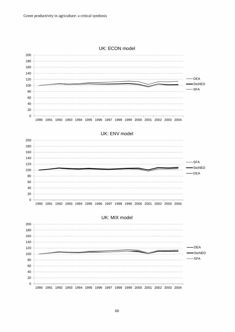
In this application we compare three alternative orientations to productivity measurement: purely economic(ECON), purely environmental (ENV), and the mixed economic and environmental (MIX). The total factorproductivity (TFP) index used in the application is the conventional Malmquist index, consisting of thetechnical change (TECH) and efficiency change (EFF) components. The frontier is estimated by the paneldata version of stochastic semi-nonparametric envelopment of data (StoNED: Kuosmanen and Kortelainen,2012) assuming monotonicity, convexity, and constant returns to scale. Technical change is captured by aparametric, linear time trend. For comparison, we will also consider the conventional SFA and DEAapproaches. In Section 7.3 we estimate the conventional Cobb-Douglas production function by SFA,specifying the most productive country as the benchmark as in Schmidt and Sickles (1984), and capturingthe technical change by a linear trend. In Section 7.4 we apply the panel data version of DEA suggested byRuggiero (2004), which is capable to assimilate stochastic noise.

The empirical analysis has been conducted using the following software packages. The StoNED model was


21

estimated using the GAMS (General Algebraic Modeling System) software and its MINOS solver (seehttp://nomepre.net/index.php/computations for further details). The SFA model was estimated using theStata software (see http://www.stata.com/). The DEA model using the EMS software (EfficiencyMeasurement System: see http://www.holger-scheel.de/ems/). See Appendix 1 for a more detaileddescription of the assumptions and properties of the DEA, SFA, and StoNED methods.

Comparable sector level data on economic inputs and outputs as well as environmental variables are notavailable for all OECD countries. Based on data availability, we have included in the cross countrycomparison 13 OECD countries: AUT, DEN, FIN, FRA, GER, GRE, ITA, NED, NOR, POR, SPA, SWE,and UK. The time span of the study is 15 years, from 1990 to 2004. Unfortunately, more recent data wereunavailable for many key variables. In future research, it would be interesting to extend the present studyto cover a larger set of countries (including non-European countries) and more recent years, provided thatcomparable data are available.

As the output variable, one could use the gross output or the value added; see OECD (2001) for a detaileddiscussion of these two approaches. In the present context, it is convenient to resort to the value addedapproach where the use of intermediate inputs is subtracted from the gross output. It is somewhatchallenging to obtain comparable data of the use of intermediate inputs at the sectoral level. Further, alarge number of input variables can cause problems for estimation, in particular, possible multicollinearityin the parametric approaches, and the so-called ‘curse of dimensionality’ in the non-parametric approaches.Therefore, in this study we use the net production value (constant 2004-2006 prices, 1 000 Int. $) reportedby FAOSTAT as the output variable y in all three alternative models. Based on the description provided byFAOSTAT, it seems that this output variable excludes the intermediate inputs (seed and feed are explicitlymentioned in the description), which are included in the gross production value reported by FAOSTAT.

The three model specifications differ in terms of the specification of the inputs.

The ECON model includes the following inputs:- Capital K (gross capital stock, constant 2005 prices, FAOSTAT),- Labour L (primary agriculture employment, number employed, OECD)- Land LA (total agricultural land area, hectares, OECD)

The ENV model includes the following variables (treated as input factors):- Agricultural total GHGs (Tonnes CO2 equivalent, OECD)- Nitrogen stock N (own calculations, based on the nitrogen surplus reported by OECD)- Phosphorus stock P (own calculations, based on the phosphorus surplus reported by OECD)- Land LA (total agricultural land area, hectares, OECD)

The model MIX contains all six input variables of both the ECON and ENV models.

The inputs of the ECON model are rather standard. Note that the land capital could be modelled as a partof the capital stock. Based on the description of FAOSTAT, the gross capital stock reported by FAOSTATonly includes the physical assets in use. Therefore, we model the land area as a separate input variable.Further, it is common to express all input and output variables proportional to the land area (e.g., outputper hectare). In fact, dividing all input variables and the output by one of the input variables effectivelyimposes the CRS assumption; we will utilize this property in Section 7.3.

The ENV model includes all environmental variables for which comparable data are available. The GHGemissions take into account the use of fossil fuels for energy, but also methane emissions from livestock.Based on the discussion in Section 5.2, we prefer to use the stocks of nitrogen and phosphorus as indicatorsof environmental pressure from nutrients use. Finally, the ENV model also includes the land area, which


22

can be considered as a part of the natural capital. A practical reason for including the land area is that wecan impose CRS consistently across all models by dividing all input variables and the output by the sameinput variable, the land area. In other words, we can express all variables on a per hectare basis.

The MIX model combines the economic and environmental perspectives, allowing us to model trade-offsand substitution possibilities between economic inputs and environmental resources explicitly. Note thatboth the ECON and ENV models are nested within the more general MIX model. The ECON model isobtained from the MIX model by restricting the shadow prices of the environmental variables as equal tozero. Similarly, the ENV model is obtained from the MIX model by setting the shadow prices of theeconomic inputs equal to zero. As a result, the empirical fit of the MIX model (measured, e.g., by thecoefficient of determination R2) is always better than that of the ECON model or that of the ENV model. Alimitation of the MIX model is that does not distinguish whether high TFP level or TFP growth is due togood performance in economic or environmental criteria. Therefore, it is useful to consider and comparethe results of all three approaches.

To gain intuition to the levels and changes in productivity in this sample of countries during the timeperiod, we first examine partial productivity measures, the average labour and capital productivity,presented in Tables 1 and 2.

Table 1: Labour productivity (y/L) in the sample countries; averages of 1990 – 2004

Country Mean y/L Efficiency rank y/L rankAUT 18.82 41 % 7 4.48 % 5DEN 46.28 100 % 1 4.55 % 4FIN 11.82 26 % 10 3.63 % 7FRA 39.40 85 % 3 4.69 % 3GER 26.52 57 % 5 4.30 % 6GRE 9.82 21 % 12 3.41 % 8ITA 20.03 43 % 6 5.76 % 1NED 45.22 98 % 2 2.33 % 11NOR 11.27 24 % 11 1.82 % 12POR 5.68 12 % 13 3.37 % 9SPA 18.77 41 % 8 5.39 % 2SWE 17.24 37 % 9 2.72 % 10UK 30.61 66 % 4 0.94 % 13Notes: The unit of measurement for labour productivity y/L is $1,000 per worker. Efficiency is calculatedas the ratio of mean labour productivity y/L of country and the mean labour productivity of Denmark,which has the highest y/L ratio in the sample. y/L is the geometric mean of the annual changes in labourproductivity y/L.

Countries are sorted in alphabetical order in Table 1: the first column indicates the country abbreviation.The second column indicates the average labour productivity in $1 000 per worker. The third columnindicates the relative labour efficiency, calculated as the ratio of country’s average labour productivity andthat of Denmark, the country with the highest labour productivity in this sample. To help a reader toquickly recognize the most productive and least productive countries, the fourth column indicates therelative rank of a country in terms of labour productivity. Observe the large differences in the level oflabour productivity across countries. For example, Greece and Portugal achieve on the average only 21%and 12% of the labour productivity of Denmark during this time period. The large differences in labourproductivity across countries are not surprising given the intensive use of capital intensive productiontechnologies in some countries in contrast to more traditional labour intensive agriculture in others.


23

Column y/L in Table 1 indicates the change in labour productivity, calculated as the geometric mean ofthe annual changes of y/L. The last column indicates the relative rank of a country in terms of labourproductivity growth. All countries achieved positive labour productivity growth during this period. Thehighest growth occurred in Italy, followed by Spain and France.

Table 2 presents the analogous statistics for capital productivity y/K. Observe the large differences in thelevel of capital productivity across countries. No other country in the sample comes even close to thecapital productivity of the Netherlands. We should add that the measurement of the capital stock is achallenging task, and the data of capital stocks reported by FAOSTAT might not be fully comparableacross countries, but in this study, we assume the FAOSTAT data are correct. As for the changes, thegrowth of capital productivity y/K is rather modest compared to the labour productivity growth. ForNorway, Sweden, and the United Kingdom, capital productivity declined during this time period. Thecomparison of Tables 1 and 2 reveals a rather different picture both in terms of the levels of productivityand the productivity growth. This highlights the need to resort to TFP measures that can accommodatemultiple input factors, including environmental factors.

Table 2: Capital productivity (y/K) in the sample countries; average of 1990 – 2004

Country Mean y/K Efficiency rank y/K rankAUT 244.6 26 % 10 1.318 % 3DEN 410.1 44 % 2 1.763 % 2FIN 136.9 15 % 12 1.059 % 5FRA 387.9 42 % 4 0.932 % 7GER 304.5 33 % 8 2.454 % 1GRE 399.7 43 % 3 0.308 % 10ITA 365.2 39 % 5 0.548 % 9NED 925.5 100 % 1 1.000 % 6NOR 132.4 14 % 13 -0.049 % 11POR 248.2 27 % 9 1.152 % 4SPA 346.1 37 % 6 0.603 % 8SWE 187.9 20 % 11 -0.275 % 12UK 338.2 37 % 7 -0.300 % 13Notes: Efficiency is calculated as the ratio of mean capital productivity y/K of country and the mean capitalproductivity of the Netherlands, which has the highest y/K ratio in the sample. y/K is the geometric meanof the annual changes in capital productivity y/K.

Analogous to labour and capital productivity, environmental partial productivity measures could becalculated using the environmental indicators noted above. Since such environmental partial productivityindicators have been reported elsewhere (see, e.g., OECD, 2008, 2011a), we turn our focus on the TFPmeasures.

7.2 Stochastic semi-nonparametric envelopment of dataWe first estimate the following log-transformed production models by convex nonparametric least squares(CNLS: Kuosmanen, 2008; Kuosmanen and Kortelainen, 2012)

ECON: ln ln ( , , )it it it it ity f K L LA Trend t

ENV: ln ln ( , , , )it it it it it ity g GHG N P LA Trend t

MIX: ln ln ( , , , , , )it it it it it it it ity h K L LA GHG N P Trend t


24

where f, g, and h are unknown monotonic increasing and concave functions that exhibits constant returns toscale, Trend is a parameter that represents Hicks neutral technical change, and it is the disturbance termthat captures both inefficiency and noise. Note that in the panel data setting the idiosyncratic errors cancelout over time. Thus, we follow Schmidt and Sickles (1984) and use the average of the residuals of the mostefficient country as the benchmark level to define the frontier. The country specific efficiency levels areestimated as the geometric mean of the residuals of country i divided by the geometric mean of theresiduals in the most efficient country

1

1

exp( )

max exp( )

TT it

ti T

T hth t

Eff .

The nonparametric estimator of the production function f is a piece-wise linear function that ischaracterized by supporting hyper-planes. The coefficients of the supporting hyper-planes can beinterpreted as marginal products of inputs. Table 3 reports summary statistics of the estimated marginalproducts in the ECON, ENV, and MIX models. Note that the marginal products vary across countries andyears.

Table 3: Marginal products of inputs in ECON, ENV, and MIX models: summary statistics of the CNLSestimates (prices of 2004 – 2006)

ECON Mean St. Dev. Min MaxK 0.1045 0.1429 0 0.3190L ($/pers.) 7 540.32 5 199.47 0 34 546.00LA ($/ha) 394.48 312.12 0 2 249.34R2 0.855

ENV Mean St. Dev. Min MaxGHG ($/ton) 194.54 167.39 0 348.71N ($/ton) 1 364.99 1 746.38 0 5 838.43P ($/ton) 1 785.50 4 572.35 0 34 941.61LA ($/ha) 249.08 101.91 0 525.76R2 0.942

MIX Mean St. Dev. Min MaxK 0.01936 0.03611 0 0.1957L ($/pers.) 3 930.84 5 502.72 0 36 216.77LA (€/ha) 103.60 135.04 0 563.97GHG ($/ton) 148.64 127.20 0 362.78N ($/ton) 1 101.25 1 132.41 0 5 394.99P ($/ton) 2 133.24 4 242.54 0 35 401.12R2 0.948

In the ECON model, the average marginal product of capital is 0.10, which means that capital investmentpays back in 10 years on average in the sample of countries considered. For some countries (e.g., Greece,Portugal) the payback period is very short, less than 4 years. For others (e.g., Norway, Finland, Sweden)the marginal product of capital is zero, which suggest these countries have overinvested in capital goods.


25

The marginal product of labour is on average 7 540 dollars per person per year. The maximum value is34 546 dollars per person per year (France 2004). Austria, Denmark, Finland, France, Germany, Norway,and Sweden achieve consistently labour productivity of more than 10 000 dollars per person. The marginalproduct of labour is lowest in Portugal, Greece, and Spain. The marginal product of agricultural land is onaverage 394 dollars per hectare. The maximum is 2 249 dollars per hectare (the Netherlands 1991). Ingeneral, the marginal products of land and labour have a high positive correlation across countries:countries that have a high marginal productivity of labour tend to have also high marginal productivity ofland. In this respect, land might be modelled as a part of the capital stock

Interestingly, the empirical fit of the ENV model is better than that of the ECON model (the R2 statisticsare 0.942 in the ENV model and 0.855 in the ECON model, respectively), even though the labour andcapital inputs are excluded. The R2 increases only marginally when the labour and capital are restored inthe MIX model. Note that the estimated average marginal product of capital is very small in the MIXmodel, and those of labour and land are also considerably smaller in the MIX model than in the ECONmodel. The estimated marginal products of GHG and the nitrogen stock also decrease when moving fromthe ENV model to the MIX model, but not dramatically. The estimated marginal product of the phosphorusstock is on average larger in the MIX model than in the ENV model. Considering both the empirical fit andthe estimated marginal products, these finding suggests that the environmental resources (GHG, N, and P)can explain empirically the observed output variations across countries and years better than the labour andcapital inputs used in the conventional production models.

Table 4 reports the parameter estimates of the time trend. The parametric trend is estimated simultaneouslytogether with the nonparametric production function f (see Johnson and Kuosmanen, 2011; 2012, fordetails). The time trend is positive and statistically significant at 5% significance level. Interpreting thetime trend as global frontier shift, the annual rate of technical progress is TECH = exp(0.016) = 1.01618,which indicates 1.618 % technical progress per year, assumed constant across all countries and years.

Table 4: Parameter estimates of the time trend; semi-nonparametric StoNED model

Model Coefficient St. error t stat p-value lower 95% upper 95%ECON 0.0160 0.0070 2.2871 0.0233 0.0022 0.0299ENV 0.0119 0.0044 2.6828 0.0079 0.0032 0.0206MIX 0.0162 0.0042 3.8614 0.0002 0.0079 0.0244

Consider next the country specific efficiency estimates obtained with the ECON, ENV, and MIX models.Both the level and change of efficiency and TFP are of interest, as well as the relative performancerankings of countries.

We start with the results of the ECON model, presented in Table 5. The 13 countries considered are listedin alphabetical order, as in Tables 1 and 2 above. The first column indicates the efficiency level, calculatedas the geometric mean of the annual efficiency estimates in years 1990 – 2004. Recall that 100% efficiencyrepresents the average efficiency of the best performing country in the sample. To help a reader to identifythe best performing countries as well as the worst performers, the second column of Table 5 indicates therelative ranking of country in terms of the efficiency level. However, the ranking of countries is not themain focus of this exercise. The third column indicates the average annual percentage change in efficiency,calculated as the geometric mean of the annual changes in the efficiency levels. The next column indicatesthe relative rank of the country in terms of the efficiency change. The rightmost column indicates theaverage TFP change, calculated as the product of the efficiency change and the technical changecomponents. For the sake of interpretation, we express the average TFP change as percentage per year,calculated using the geometric mean of the TFP change between immediately adjacent years. Since the


26

technical change is assumed to be constant across all countries and years, the relative ranking of TFPchanges is exactly the same as the efficiency change ranking.

Table 5: Efficiency levels, efficiency change, and TFP change according to the ECON model; Semi-nonparametric StoNED estimates

EFF level Rank EFF change Rank TFP changeAUT 31 % 9 1.060 % 1 2.695 %DEN 64 % 2 0.852 % 3 2.484 %FIN 20 % 13 0.396 % 6 2.021 %FRA 45 % 3 0.440 % 5 2.065 %GER 44 % 4 0.674 % 4 2.302 %GRE 42 % 5 -1.279 % 12 0.318 %ITA 41 % 6 0.915 % 2 2.548 %NED 100 % 1 -0.138 % 7 1.477 %NOR 23 % 12 -0.733 % 10 0.873 %POR 26 % 10 -0.460 % 9 1.150 %SPA 36 % 8 -0.927 % 11 0.676 %SWE 25 % 11 -0.340 % 8 1.272 %UK 37 % 7 -1.391 % 13 0.204 %Note: Global technical change (TECH) is estimated as 1.618 % for all countries and years

In the ECON model, the Netherlands is by a large margin the most efficient country in transformingeconomic inputs to agricultural value added in the sample of countries considered (compare with Table 2).The efficiency levels are scaled relative to the average performance of the Netherlands. Denmarkdistinguishes itself as the second most efficient agricultural producer after the Netherlands (recall thatDenmark had the highest labour productivity in Table 1). The other Nordic countries, Finland, Norway,and Sweden, are the least efficient countries in the sample.

The global technical progress is estimated as 1.618 % across all countries and years. All countries achievepositive TFP growth according to the ECON model. The largest growth (catching up) is achieved inAustria, Italy, and Denmark. Efficiency change is negative (falling behind) in the United Kingdom,Greece, Spain, Norway, Portugal, Sweden, and the Netherlands. This group includes both the mostefficient producer (NED), but also some of the least efficient producers (NOR, SWE). There are somesigns of catching up the lead of the Netherlands, most notably in Austria, Italy, and Denmark, but also inGermany, France, and Finland. The country specific TFP trajectories are presented in Appendix 2, to bediscussed in more detail in Section 7.5.

Table 6 presents the analogous results for the ENV model. In this case, the subset of environmental inputsis included in the model, and the economic inputs (labour, capital) are excluded. Recall from Table 3 thatthe empirical fit of the ENV model is better than that of the ECON model.

In terms of the levels, Italy is the most environmentally efficient producer according to the ENV model inthis sample, followed by the Netherlands. The differences in the levels of environmental efficiency remainlarge, but not as dramatic as in the ECON model. Sweden, Finland and Norway are among the leastefficient countries also in terms of the ENV model.

Regarding the changes, Italy also shows the highest average rate of efficiency improvement, while Norwayhas relatively large efficiency decline. The high positive correlation between the levels and changes inenvironmental efficiency suggests that countries diverge rather catch up in terms of their environmental


27

performance. However, when we take the technical progress (on average 1.2% per year) into account, theenvironmental TFP growth is positive in all countries, except for Norway. For most countries, the averageenvironmental TFP growth falls below the economic TFP growth.

Table 6: Efficiency levels, efficiency change, and TFP change according to the ENV model; Semi-nonparametric StoNED estimates

EFF level Rank EFF change Rank TFP changeAUT 72 % 4 0.750 % 4 1.955 %DEN 70 % 5 1.130 % 2 2.341 %FIN 43 % 12 0.637 % 6 1.841 %FRA 64 % 7 0.787 % 3 1.994 %GER 64 % 6 0.016 % 7 1.213 %GRE 75 % 3 0.638 % 5 1.842 %ITA 100 % 1 1.511 % 1 2.726 %NED 88 % 2 -0.139 % 8 1.056 %NOR 41 % 13 -1.676 % 13 -0.499 %POR 61 % 9 -1.108 % 12 0.075 %SPA 62 % 8 -0.668 % 11 0.521 %SWE 50 % 10 -0.402 % 9 0.790 %UK 45 % 11 -0.632 % 10 0.558 %Note: Global technical change (TECH) is estimated as 1.197 % for all countries and years

Table 7: Efficiency levels, efficiency change, and TFP change according to the MIX model; Semi-nonparametric StoNED estimates


Finally, consider the mixed economic and environmental (MIX) model. The efficiency levels and changesand the overall TFP changes are reported in Table 7. Overall, the results are rather similar to those of Table6. This is not surprising keeping in mind the fact that the empirical fit does not increase much when wemove from the ECON model to the MIX model. Italy and the Netherlands are again the most efficientcountries, and Finland and Norway are the least efficient ones. The average rates of changes in TFP arehigher in the MIX model than in the ENV model for all countries, and the levels of efficiency are alsohigher in the MIX model for all countries except for Greece and Portugal. This is expected since the MIX


28

model includes a larger number of input variables, and hence it must have a better empirical fit than theENV model.

In conclusion, the ECON and ENV models show performance of some countries in rather different light:consider, for example, Italy and the Netherlands. The results of the MIX model lean towards the ENVmodel. We find that all three orientations work reasonably well in the context of semi-nonparametricStoNED estimation, providing results that are in line with the partial productivity measures reported aboveand the results of the SFA and DEA estimators to be discussed next. The MIX model can provide areasonable combination of the ECON and ENV models. However, it could be argued that the orientation ofthe MIX model can blur the interpretation of the ECON and ENV models. In this application, the MIXmodel seems to provide little additional value to the purely environmental ENV model.

7.3 Parametric SFA

For comparison, we repeat the previous analysis, imposing the Cobb-Douglas functional form for thefrontier. Thus, the model can be estimated by standard least squares techniques. Specifically, we follow thepanel data approach to SFA by Schmidt and Sickles (1984). The CRS assumption is imposed by dividingall input variables by the agricultural land area (thus all variables are expressed per hectare). The ECONmodel can be stated in the log-linear form as

ECON: 0ln( / ) ln( / ) ln( / )it it K it it L it it ity LA K LA L LA Trend t

ENV: 0ln( / ) ln( / ) ln( / ) ln( / )it it GHG it it N it it P it it ity LA GHG LA N LA P LA Trend t

MIX: 0ln( / ) ln( / ) ln( / )ln( / ) ln( / ) ln( / )

it it K it it L it it

GHG it it N it it P it it it

y LA K LA L LAGHG LA N LA P LA Trend t

In the ECON model, the output elasticity of land can be obtained as 1 ( )K L . The time trendrepresents the technical change of the global frontier, which is constant across all countries and timeperiods. The coefficients estimated by OLS and the standard errors and other supporting statistics arereported in Table 8.

In the ECON model, the coefficients of K and L are positive and statistically significant at 5% significancelevel. The output elasticity of land is 0.321. The time trend is positive and of the expected magnitude(TECH = 1.0122, implying 1.22% technical progress per annum), but it is statistically insignificant. Theempirical fit of the ECON model is rather poor, the coefficient of determination is only 0.214. The modelas a whole is still highly significant in the F-test.

The ENV model achieves a much better empirical fit: the coefficient of determination is 0.665. Allcoefficients are positive, and the coefficients of GHG and N stock are significant, while the coefficient ofthe P stock is insignificant. The output elasticity of land is 0.188. The time trend is positive and significant:TECH = 1.0156, implying 1.56% technical progress per year.

The MIX model must obviously have a better empirical fit than the ENV model. However, the coefficientof determination increases only marginally to 0.689. The increase is not statistically significant. Further,the MIX model provides somewhat counterintuitive results. The coefficient of capital K becomes negative,but insignificant, whereas in the ECON model it was positive and highly significant. The coefficients ofGHG and N do not change dramatically compared to the ENV model. The time trend is positive andstatistically significant in the MIX model.


29

Table 8: The results of the ECON, ENV, and MIX models estimated by OLS

ECON Coefficient St. error t stat p-value lower 95% upper 95%Constant 3.455 0.485 7.126 0.000 2.499 4.412K/LA 0.524 0.097 5.386 0.000 0.332 0.716L/LA 0.154 0.073 2.114 0.036 0.010 0.298Trend 0.012 0.008 1.499 0.136 -0.004 0.028R2 0.214

ENV Coefficient St. error t stat p-value lower 95% upper 95%Constant 0.881 0.120 7.368 0.000 0.645 1.117GHG/LA 0.174 0.049 3.548 0.000 0.077 0.270N/LA 0.578 0.073 7.954 0.000 0.435 0.721P/LA 0.061 0.066 0.917 0.361 -0.070 0.191time 0.015 0.005 2.991 0.003 0.005 0.026R2 0.665

MIX Coefficient St. error t stat p-value lower 95% upper 95%Constant 0.728 0.359 2.030 0.044 0.021 1.436K/LA -0.103 0.080 -1.285 0.200 -0.260 0.055L/LA 0.182 0.047 3.857 0.000 0.089 0.275GHG/LA 0.211 0.049 4.344 0.000 0.115 0.307N/LA 0.548 0.071 7.755 0.000 0.409 0.688P/LA 0.076 0.072 1.058 0.291 -0.066 0.217Trend 0.020 0.005 3.958 0.000 0.010 0.031R2 0.689

In conclusion, the ENV model achieves much better empirical fit than the ECON model. The MIX modeldoes not add significantly to the explanatory power of the ENV model, and the coefficient of capital Kbecomes negative in the MIX model. This illustrates problems associated with the MIX model. In ourview, separate modelling of ECON and ENV models is preferred, whereas the MIX approach tends toobscure the interpretation and lead to counterintuitive results.

Consider next the country specific efficiency estimates obtained with the ECON, ENV, and MIX models.Both the level and change of efficiency and TFP are of interest, as well as the relative performancerankings of countries.

We start with the results of the ECON model, presented in Table 9, prepared analogous to Tables 5 – 7presented above.

In the ECON model, the Netherlands is by a large margin the most efficient country, similar to the StoNEDresults presented and discussed above. The efficiency levels are scaled relative to the average performanceof the Netherlands. In this comparison, no other country can achieve even 50% of the performance level ofthe Netherlands. The least efficient countries are Finland, Norway, and Sweden. We note that the SFAestimates of both the levels of efficiency and the relative country rankings are almost perfectly correlatedwith the StoNED estimates (the correlation coefficient of efficiency levels is 0.979). Although theempirical fit of the parametric SFA model is considerably lower than that of the semi-nonparametricStoNED, the efficiency estimates are almost identical.


30

Table 9: Efficiency levels, efficiency change, and TFP change according to the ECON model; Cobb-Douglas production function estimated by OLS

EFF level Rank EFF change Rank TFP changeAUT 25 % 9 0.388 % 5 1.617 %DEN 46 % 2 0.663 % 3 1.895 %FIN 16 % 13 -0.064 % 8 1.160 %FRA 38 % 3 0.149 % 6 1.375 %GER 34 % 5 0.708 % 1 1.941 %GRE 28 % 7 -0.109 % 9 1.115 %ITA 37 % 4 0.663 % 2 1.896 %NED 100 % 1 -0.317 % 10 0.904 %NOR 17 % 12 -1.268 % 13 -0.059 %POR 20 % 10 0.131 % 7 1.357 %SPA 28 % 8 0.493 % 4 1.724 %SWE 20 % 11 -0.937 % 11 0.276 %UK 31 % 6 -1.143 % 12 0.068 %Note: Global technical change (TECH) is estimated as 1.225 % for all countries and years

The global technical progress is estimated as 1.225 % across all countries and years. The largest growth(catching up) is achieved in Germany, Italy, and Denmark. Efficiency change is negative (falling behind)in Norway, UK, Sweden, Netherlands, Greece, and Finland. This group includes both the most efficientproducer (NED), but also the two least efficient producers (FIN, NOR). The SFA estimates of efficiencychange are also almost perfectly correlated with the StoNED estimates (the correlation coefficient ofannual country-specific efficiency changes is as high as 0.974), but the average rates of efficiency changeand the relative rankings are not exactly identical. The differences in the overall TFP estimates are mainlydue to the time trend, where the SFA estimate (1.225% per year) is notably lower than the StoNEDestimate (1.618% per year).

Table 10: Efficiency levels, efficiency change, and TFP change according to the ENV model; Cobb-Douglas production function estimated by OLS


The SFA estimates of the ENV model are presented in Table 10. As in the StoNED model, Italy is the most


31

efficient country with a clear margin to the Netherlands. Italy is also improving its environmentalperformance over time faster than any other country in the sample. The total environmental performancechange is positive to all countries, except for Norway, thanks to the relatively large technical progresscomponent (1.558% per year, which is constant across all countries and years). The SFA model supportsour earlier conclusion that countries appear to divergence in their environmentally performance over time,as the inefficient countries are lagging behind. Indeed, the SFA estimates of the ENV model are highlycorrelated with the corresponding StoNED estimates: the correlation coefficient of the efficiency levels is0.916, and the correlation of the annual country-specific efficiency changes is 0.919. In the ENV model,the SFA estimate of the technical change (1.558% per year) is higher than the corresponding StoNEDestimate (1.197% per year). This explains the high average rates of the TFP change in the SFA model.

Finally, the results of the MIX model are presented in Table 11. Similar to the ENV model, Italy is themost efficient country in the MIX model, with largest efficiency improvement. Somewhat surprisingly, theNetherlands (the 1st in the ECON model and the 2nd in the ENV model) falls now to the fourth positionafter Austria and Denmark. However, the efficiency level of the Netherlands does not change dramaticallycompared to the ENV model. The least efficient countries are again Norway, the United Kingdom, andFinland. Overall, the country specific efficiency results of the MIX model are rather similar to those of theENV model. Moreover, the SFA estimates of the MIX model are highly correlated with the correspondingStoNED estimates: the correlation coefficient of the efficiency levels is 0.934, and the correlation of annualcountry-specific efficiency changes is 0.981. However, the SFA estimate of technical change (2.067% peryear) is considerably larger than the corresponding StoNED estimate (1.629). This shows in the largeestimates of the overall TFP change reported in Table 11.

Table 11: Efficiency levels, efficiency change, and TFP change according to the MIX model; Cobb-Douglas production function estimated by OLS


In conclusion, the SFA and StoNED estimates provide a very similar picture of both the levels and changesof efficiency. However, the estimates of technical change (TECH) component reveal larger differences.Somewhat surprisingly, the parametric trend function proves more sensitive to the functional formassumption (i.e., the Cobb-Douglas specification) than the regression residuals and their country-specificaverages in this particular application. It is possible that the linear trend function, which assumes Hicksneutral technical change, is a too restrictive specification of technical progress. More flexible specificationsof technical change might be preferable in this case, but exploring this issue further falls beyond the scopeof the present study.


32

7.4 Stochastic DEA

The conventional approach to applying DEA in the context of the Malmquist index is to treat the panel ofcountries as yearly cross sections that are completely independent of each other. This approach ignores theinter-temporal nature of the panel data. Ruggiero (2004) has proposed an alternative approach to applyingDEA to panel data, which is more consistent with the StoNED and SFA approaches considered above.More specifically, Ruggiero first computes country-specific averages of inputs and outputs over the timeperiods included in the panel. He then proposes to apply DEA to thus obtained country averages. In thisway, random variations from one year to another get averaged out from the input-output data. Hence,Ruggiero’s approach is less sensitive to idiosyncratic noise than the conventional DEA. Ruggiero refers tohis method as “stochastic DEA”, and presents some simulation evidence in support of the method. Thepresent study forms one of the first empirical applications of this method.

Since the performance of countries is measured relative to the fixed-base inter-temporal frontier spannedby the country-specific average values, we cannot distinguish between the efficiency change and technicalchange components in this method. However, we can measure TFP changes in terms of the change of thedistance function (or efficiency index) over time.

Table 12 reports the DEA estimates of efficiency levels and the TFP changes in the ECON model. TheNetherlands and Denmark are ranked as efficient countries in the DEA assessment. The efficiencydifferences across countries are large: Finland and Norway achieve only 26% and 25% efficiency levels,respectively, compared to the most efficient countries. The DEA efficiency estimates are positivelycorrelated with the StoNED and SFA estimates (the correlation coefficients: DEA and StoNED 0.850,DEA and SFA 0.784).

Table 12: Efficiency levels and TFP change according to the ECON model; inter-temporal productionfunction estimated by stochastic DEA

EFF level Rank TFP change RankAUT 41 % 8 4.48 % 3DEN 100 % 1 4.55 % 2FIN 26 % 12 3.63 % 7FRA 85 % 3 4.69 % 1GER 57 % 5 4.30 % 4GRE 43 % 6 0.31 % 13ITA 43 % 7 4.04 % 5NED 100 % 1 1.29 % 10NOR 25 % 13 1.82 % 9POR 27 % 11 1.15 % 11SPA 40 % 9 3.73 % 6SWE 38 % 10 2.72 % 8UK 68 % 4 0.94 % 12Note: Ruggiero’s (2004) inter-temporal panel data DEA approach does not allow us to separate TFPchange to efficiency change and technical change components

In general, the DEA estimates of TFP change reported in Table 12 are notably higher than thecorresponding StoNED or SFA estimates. At this point, it is worth to emphasize that the average TFPgrowth rates reported for StoNED and SFA in Sections 7.2 and 7.3 were calculated using the chain indexmethod where the value of any given period is compared to the value of its immediately preceding period.In contrast, the DEA estimates have been calculated relative to a fixed base period, since the DEA frontier


33

is estimated using the average input-output data. Unfortunately, the Malmquist TFP index does not satisfythe circularity test (e.g., Pastor and Lovell, 2007). This means that individual indices cannot be consistentlychained together by multiplying consecutive indices to convert them to some desired reference period:multiplying a chain of Malmquist TFP indices between the base period 0 and all consequtive periods untilperiod t will generally yield a different result than the direct comparison between periods t and 0. Thisproperty of the Malmquist index can partly explain why the DEA estimates of the TFP change reported inTable 12 are higher than those reported for StoNED and SFA above.

The evolution of the comparable fixed base period TFP indices is presented graphically in Appendix 2 (tobe discussed in more detail in Section 7.5). The general impression from these figures is that DEA tends toindicate higher TFP growth rates than the corresponding StoNED and SFA estimates. It appears that theDEA estimates are mainly driven by labour productivity growth (compare with Table 1), whereas theslower growth of capital productivity (Table 2) is given less weight in the DEA assessment. Recall that themain principle of DEA is to look at performance of countries in the most favourable light.

Consider next the DEA estimates of the ENV model reported in Table 13. In this model, it is clear thatDEA suffers from low discriminating power: five countries are classified as 100% efficient (AUT, GRE,ITA, NED, and SPA). In particular, efficiency of Greece is a surprising result since Greece ranks relativelylow in all other tables presented above. Only Finland and Norway are assigned similar (low) efficiencyscores as in StoNED and SFA, all other countries are given the ‘benefit of the doubt’.

Table 13: Efficiency levels and TFP change according to the ENV model; inter-temporal productionfunction estimated by stochastic DEA

EFF level Rank TFP change RankAUT 100 % 1 2.36 % 4DEN 82 % 6 2.60 % 3FIN 44 % 13 2.13 % 6FRA 74 % 7 2.33 % 5GER 70 % 8 1.83 % 7GRE 100 % 1 2.69 % 2ITA 100 % 1 3.00 % 1NED 100 % 1 1.00 % 9NOR 45 % 12 -0.08 % 11POR 65 % 10 -0.12 % 12SPA 100 % 1 -0.44 % 13SWE 65 % 9 1.52 % 8UK 49 % 11 0.33 % 10Note: Ruggiero’s (2004) inter-temporal panel data DEA approach does not allow us to separate TFPchange to efficiency change and technical change components

The DEA estimates of the TFP change in the ENV model are reasonably well in line with the StoNED andSFA estimates. However, it worth to note the trade-off between the explanatory power (i.e., empirical fit)and the discriminating power of DEA. While the discriminatory power of DEA proved low in terms of thelevels of efficiency, the empirical fit of the ENV model is much better than that of the ECON model, whichexplains why the estimates of TFP change are more consistent with the StoNED and SFA estimates.

Finally, the DEA estimates of the MIX model are reported in Table 14. This table highlights the difficultyof DEA to discriminate between countries as the number of input-output variables increases. Sevencountries (more than half of the sample) are classified as 100% efficient. Similar to the ENV model, the


34

low discriminating power implies good empirical fit, which in turn results as estimates of TFP change thatare reasonably well in line with the corresponding StoNED and SFA estimates.

Table 14: Efficiency levels and TFP change according to the MIX model; inter-temporal productionfunction estimated by stochastic DEA

EFF level Rank TFP change RankAUT 100 % 1 2.63 % 7DEN 100 % 1 3.96 % 1FIN 51 % 12 3.04 % 4FRA 100 % 1 3.07 % 3GER 81 % 8 3.00 % 5GRE 100 % 1 2.68 % 6ITA 100 % 1 3.28 % 2NED 100 % 1 1.29 % 9NOR 45 % 13 -0.08 % 13POR 66 % 11 0.20 % 12SPA 100 % 1 0.37 % 11SWE 72 % 9 1.94 % 8UK 68 % 10 0.94 % 10Note: Ruggiero’s (2004) inter-temporal panel data DEA approach does not allow us to separate TFPchange to efficiency change and technical change components

In conclusion, the above results highlight the trade-off between explanatory power and discriminatorypower of DEA. In the ECON model the discriminatory power of efficiency estimates was reasonably good,but then the DEA frontier is spanned by two observations only. This results as poor empirical fit, and theestimates of TFP change are much higher than those obtained with other methods. In the ENV and MIXmodels, however, the discriminating power of DEA proves poor, but the estimates of TFP change are morereasonable.

Regarding the choice of the method, we find that results of the StoNED, SFA, and DEA differ notably. Itcan be objectively shown that the models are nested in the sense that both DEA and SFA can be obtainedas restricted special cases of the more general StoNED model (Kuosmanen and Johnson, 2010; Kuosmanenand Kortelainen, 2012). The general principle in statistical testing of restrictions is that if two nestedmodels do not exhibit significant differences, then then the assumptions of the restricted model can bemaintained, whereas if the two models exhibit significant differences, the assumptions of the restrictedmodel are rejected and the more general model is chosen. Unfortunately, statistical testing of models thathave been estimated using nonparametric methods is not straightforward, as the degrees of freedom are notwell defined. One might apply the bootstrap method, but to our knowledge, the statistical consistency ofthe bootstrap method for this particular purpose has not be established. Therefore, we conclude that thedifferences between methods appear to be economically significant, but we leave the statisticalsignificance tests for future research.

7.5 Evolution of country specific TFP measures over time

Based on the average TFP levels and the average rates of TFP growth examined in the previous sub-sections, it may appear that the TFP estimates are sensitive to the specification of economic andenvironmental resources and to the choice of the estimation method. Indeed, the efficiency levels and therelative country rankings are highly dependent on the criteria used in the efficiency assessment, theweights assigned to the criteria, and the weighting method used.


35

Often the main focus of productivity analysis is on the development of TFP over time. Thus far, we haverestricted attention the average growth rates of TFP, which can be conveniently summarized in tables.However, the evolution of country specific TFP trends is worth investigating in more detail. To this end,the fixed-base TFP indices (1990=100) according to the ECON, ENV, and MIX models, estimated byStoNED, SFA and DEA, are plotted for all countries included in this study in Appendix 2.

Appendix 2 contains 3 × 13 = 39 figures in total, so we cannot comment on each figure in detail. However,some empirical observations are worth noting.

The TFP indices of Austria and Denmark reveal relatively strong and consistent growth, irrespective ofwhether TFP is measured using economic or environmental criteria. The figures of France and Germanyindicate temporary decline in productivity during the first half of the 1990’s, but since the mid-1990s thegrowth rates are relatively high. Similarly, Finland and Sweden exhibited relatively high TFP growth aftertheir EU membership in 1995 (the EU membership apparently caused some temporary shocks, whichappear earlier in the TFP figures of Sweden than in those of Finland). Interestingly, for Greece and Italythe environmentally oriented TFP indices show considerably higher TFP growth than the purely economicTFP measure. In contrast, for Norway and Spain the economic TFP index indicates higher growth than theenvironmental TFP measure. The Netherlands exhibits relatively stable but rather modest growth. ForPortugal and the United Kingdom, the growth rate is close to zero, while in Norway the environmentallyoriented TFP indices indicate productivity decline.

To conclude, two general remarks regarding the models and methods based on the figures presented inAppendix 2 are the following.

First, the TFP indices appear to be much more robust to the specification of the economic andenvironmental inputs (i.e., ECON, ENV, or MIX specification) than the estimated levels of TFP orefficiency. The ECON, ENV, and MIX models exhibit very similar inter-temporal patterns for allcountries: similar growth trends and temporary shocks can be recognized in the TFP indices based on allthree models. For many countries, however, the ECON model indicates higher TFP growth than the ENVor MIX models, particularly if one compares the DEA estimates.

Second, the TFP indices are also relatively robust to the choice of the estimation method. For manycountries, the TFP indices computed based on the StoNED, SFA, and DEA distance functions are hardlydistinguishable from the figure, particularly in the ENV and MIX models. The most notable differencesdue to the estimation method are found in the case of the ECON model, particularly for Austria, Denmark,Finland, France, Greece, and Spain. The large deviations particularly in the ECON model are explained bythe fact that the ECON model yields lower empirical fit than the ENV and MIX models.

8. Concluding remarks and recommendations

This report addresses the following three issues. First, we presented a critical survey of literatureconsidered relevant to the measurement and analysis of productivity and environmental efficiency inagriculture. Due to the limited scope of this study, we have certainly ignored many important studies worthciting, but we find that this limited survey nevertheless provides several valuable insights to this topic.Second, we examined the methodological options available, both some well-established and widely appliedapproaches and some new approaches that have been just recently introduced or are currently beingintroduced to the literature. Third, we conducted an empirical comparison of some of the methodologicaloptions suggested. The empirical comparison provided several valuable lessons, as discussed in theprevious section.


36

Based on the insights and results obtained in this study, the following recommendations are proposed.

Firstly, we propose to draw a clear conceptual distinction between the environmentally oriented efficiencyanalysis (abbreviated as ENV above) where the economic resources are omitted, and the mixed economicand environmental orientation (abbreviated as MIX above) where both economic and environmentalresources are considered. In particular, we find it somewhat misleading to call the latter approach “eco-efficiency” or “environmental efficiency”. In our view, if one is mainly interested in environmental or eco-efficiency, efficient use of labour or capital resources seems a poor excuse for weak performance in theenvironmental criteria. Following the usual notion of eco-efficiency, environmental efficiency concerns inour interpretation the trade-off between economic goods and environmental bads. From the welfare pointof view, however, it is perfectly valid to combine the economic and environmental criteria in a commonframework of productivity assessment. The mixed economic and environmental orientation can provide auseful overall measure of productivity from the welfare point of view, which can credit countries foradvances in both economic and environmental efficiency.

Secondly, we discussed model specification issues related to agricultural production, including the damagecontrol inputs, material balance, and production risk. All these issues are obviously relevant toenvironmental efficiency. In this report we paid particular attention on the material balance discussion,which is commonly used in the calculation of the nutrient emissions, most notably the nitrogen andphosphorus. We noted that if the production model consists solely of inputs and outputs governed by thematerial balance, then the production model reduces to the material balance equation and becomesredundant. To break the direct link between material input and output, we proposed to omit some of thevariables that (almost) perfectly correlated with other variables. For example, the total energy input and theGHG tend to be so highly correlated that one could harmlessly omit one of them.

Another important issue related to the material balance concerns the use of nutrient surplus as anenvironmental indicator in productivity analysis. A problem with the conventional surplus measures is thatthe surplus is measured on the interval scale, and hence, it can yield negative values. However,productivity and efficiency measurement generally requires ratio scale variables in order to performmultiplication and division operations. To resolve this issue, we resorted to a dynamic model of materialbalance, in which the accumulation of nutrients is modelled similar to the usual perpetual inventorymethod for calculating the capital stock. It is standard to use the capital stock rather than investment (thecorresponding flow variable) as an input in productivity measurement. Analogously, in the empirical studyreported above we applied the stocks of nitrogen and phosphorus as environmental resources to production.

Thirdly, we considered a generic stochastic semi-nonparametric model of production that contains theconventional parametric-stochastic and nonparametric-deterministic models as its special case. We brieflyreviewed the conventional frontier estimation techniques, DEA and SFA, and the recently introducedStoNED method. A more detailed description of the assumptions and properties of these methods ispresented in Appendix 1. For comparison, all three approaches were applied in the empirical work reportedabove.

The comparison of the empirical results obtained in the three alternative model specifications – ECON,ENV, and MIX – obtained with three alternative frontier methods – StoNED, SFA, and DEA – reveals thefollowing insights. The empirical fit of the ENV model proved better than that of the ECON modelirrespective of the estimation method. The results of the MIX model followed relatively closely those ofthe ENV model in StoNED and SFA. The StoNED estimates of the marginal products, efficiency levels,and the efficiency and TFP changes appear reasonable in all three model specifications considered. TheSFA estimates of the efficiency levels and changes were almost perfectly correlated with the correspondingStoNED estimates, but TFP changes differ to some extent due to the technical change component. Theparameter estimates of the SFA models were reasonable in the ECON and ENV models, but in the MIX


37

model the capital input has the negative sign. Depending on the model specification, the DEA approachyields reasonable estimates of either the efficiency levels, or the TFP change, but not both. Based on thesefindings, we conclude there is a trade-off between the discriminatory power and the explanatory power ofDEA.

While this report reviews and cites a large number of studies relevant to the theme, the relevant literature isso vast that a number of potentially important and relevant works have necessarily been omitted, as werecognized already in the introduction. We have considered a limited number of index numbers, estimationmethods, model specification issues, and empirical issues considered relevant to the theme to be able toform a synthesis. This will necessarily mean that some important issues and results that do not directly fitinto our synthesis have to be omitted. Extending the synthesis presented in this report provides fruitfulavenues for further investigation.

In the similar vein, the empirical work reported in this study is necessarily limited by data availability andtime constraints. The number of countries and time periods covered in the study could be extended in thefuture research. Further, the scope of environmental issues covered deserves to be extended. A number ofimportant environmental issues were omitted from the application due to data availability, including thewater stress and discharge of toxic pesticides. These observations highlight the need for future research onthis topic.


38

References

Afriat, S. (1972) Efficiency Estimation of Production Functions, International Economic Review 13(3),568–598.

Aigner, D.J., C.A.K. Lovell, and P. Schmidt (1977) Formulation and Estimation of Stochastic FrontierModels, Journal of Econometrics 6, 21-37.

Alvarez A., Amsler, C., Orea, L., and P. Schmidt (2006) Interpreting and testing the scaling property inmodels where inefficiency depends on firm characteristics, Journal of Productivity Analysis 25, 201-212.

Andor, M., and F. Hesse (2013) The StoNED Age: The Departure Into a New Era of Efficiency Analysis? AMonte Carlo Comparison of StoNED and the “Oldies” (SFA and DEA), Ruhr Economic Papers #394,available online at: http://dx.doi.org/10.2139/ssrn.2200837.

Asche, F. (2011) Green Growth in Fisheries and Aquaculture, report to the OECD, available online at:http://www.oecd.org/greengrowth/sustainable-agriculture/48258799.pdf

Ayres, R.U., and A.V. Kneese (1969) Production, Consumption and Externalities, American EconomicReview 59, 282-297.

Balk, B.M. (1993) Malmquist Productivity Indexes and Fisher Ideal Indexes: Comment. Economic Journal103, 680–682.

Balk, B.M. (1998) Industrial Price, Quantity, and Productivity Indices: The Micro-Economic Theory andan Application. Boston, Dordrecht, London: Kluwer.

Ball, V.E., J.-C. Bureau, J.-P. Butault, and R. Nehring (2001) Levels of Farm Sector Productivity: AnInternational Comparison, Journal of Productivity Analysis 15(1), 5-29.

Ball, V.E., C. Hallahan, and R. Nehring (2004) Convergence of Productivity: An Analysis of the Catch-upHypothesis within a Panel of States, American Journal of Agricultural Economics 86, 1315-1321.

Ball, V.E., C.A.K. Lovell, R. Nehring and H. Luu (2004) Incorporating Environmental Impacts in theMeasurement of Agricultural Productivity Growth, Journal of Agricultural and Resource Economics 29,436-60.

Banker, R.D., and A. Maindiratta (1992) Maximum Likelihood Estimation of Monotone and ConcaveProduction Frontiers, Journal of Productivity Analysis 3, 401-415.

Battese, G.E., and Coelli. T.J. (1995) A model for technical inefficiency effects in a stochastic productionfrontier for panel data, Empirical Economics 20(2), 325-332.

Baumgärtner, S. (2004) The Inada Conditions for Material Resource Inputs Reconsidered, Environmentaland Resource Economics 29, 307-322.

Bjurek, H. (1996) The Malmquist Total Factor Productivity Index, Scandinavian Journal of Economics98(2), 303-313.

Blandford, D. (2011) The Contribution of Agriculture to Green Growth, report to the OECD, availableonline at: http://www.oecd.org/greengrowth/sustainable-agriculture/48258861.pdf


39

Brümmer, B., T. Glauben, and G. Thijssen (2002) Decomposition of Productivity Growth Using DistanceFunctions: The Case of Dairy Farms in Three European Countries, American Journal of AgriculturalEconomics 84(3), 628-644.

Bureau, J.-C., R. Färe, and S. Grosskopf (1995) A Comparison of Three Nonparametric Measures ofProductivity Growth in European and United States Agriculture, Journal of Agricultural Economics 46(3),309–326.

Burrell, A. (2011) Renewable Energies from the Rural Sector: The Policy Challenges, report to the OECD,available online at: http://www.oecd.org/greengrowth/sustainable-agriculture/48309185.pdf

Carpentier, A., and R.D. Weaver (1997) Damage Control Productivity: Why Econometrics Matters.American Journal of Agricultural Economics 79:47–61.

Caves, D.W., L.R. Christensen, and W.E. Diewert (1982) The Economic Theory of Index Numbers and theMeasurement of Input, Output and Productivity, Econometrica 50, 1393–1414.

Chambers, R.G., Y. Chung, and R. Färe (1996) Benefit and Distance Functions, Journal of EconomicTheory 70, 407–419.

Chambers, R.G., Y. Chung, and R. Färe (1998) Profit, Directional Distance Functions and NerlovianEfficiency, Journal of Optimization Theory and Applications 98(2), 351–364.

Chambers, R.G., and J. Quiggin (1998) A State-Contingent Production Approach to Principal-AgentProblems with an Application to Point-Source Pollution Control, Journal of Public Economics 70(3), 441–472.

Chambers, R.G., and J. Quiggin (2000) Uncertainty, Production, Choice, and Agency: The State-Contingent Approach, Cambridge University Press. 373 p.

Charnes, A., W.W. Cooper and E. Rhodes (1978) Measuring the Efficiency of Decision Making Units.European Journal of Operational Research 2(6), 429–444.

Cherchye, L., W. Moesen, N. Rogge, and T. Van Puyenbroeck (2007) An Introduction to ‘Benefit of theDoubt’ Composite Indicators, Social Indicators Research 82(1), 111-145.

Chung, Y., R. Färe, and S. Grosskopf. (1997) Productivity and Undesirable Outputs: A DirectionalDistance Function Approach. Journal of Environmental Management 51(3), 229–240.

Coelli, T.J., Lauwers, L., and G. Van Huylenbroeck (2007) Environmental Efficiency Measurement andthe Material Balance Condition, Journal of Productivity Analysis 28, 3-12.

Coelli, T.J., and D.S. Prasada Rao (2005) Total Factor Productivity Growth in Agriculture: A MalmquistIndex Analysis of 93 Countries, 1980–2000, Agricultural Economics 32(s1), 115–134.

Cox, T.L., and J.-P. Chavas (1990) A Nonparametric Analysis of Productivity: The Case of USAgriculture, European Review of Agricultural Economics 17(4), 449-464.

Cropper, M.L., and W.E. Oates (1992) Environmental Economics: A Survey. Journal of EconomicLiterature 30, 675–740.


40

Daly, H.E. (1997) Georgescu-Roegen versus Solow/Stiglitz, Ecological Economics 22, 261-266.

Debreu, G. (1951) The coefficient of resource utilization, Econometrica 19, 273–292.

Diewert, W.E. (1992) Fisher Ideal Output, Input and Productivity Indexes Revisited, Journal ofProductivity Analysis 3(3), 211–248.

Diewert, W.E. and A.O. Nakamura (2003) Index Number Concepts, Measures and Decompositions ofProductivity Growth, Journal of Productivity Analysis 19(2–3), 127–159.

Ebert, U., and H. Welsch (2007) Environmental Emission and Production Economics: Implication of theMaterial Balance, American Journal of Agricultural Economics 89, 287-293.

Färe, R. and S. Grosskopf (1992) Malmquist Productivity Indexes and Fisher Ideas Indexes, EconomicJournal 102, 158–160.

Färe, R. and S. Grosskopf (2003) Non-parametric Productivity Analysis with Undesirable Outputs:Comment, American Journal of Agricultural Economics 85, 1070–74.

Färe, R., S. Grosskopf, M. Norris and Z. Zhang (1994) Productivity Growth, Technical Progress, andEfficiency Change in Industrialized Countries, American Economic Review 84(1), 66–83.

Fan, S., and X. Zhang (2002) Production and Productivity Growth in Chinese Agriculture: New Nationaland Regional Measures, Economic Development and Cultural Change 50(4), 819-838.

Fan, Y., Q. Li, and A. Weersink (1996) Semiparametric Estimation of Stochastic Production FrontierModels, Journal of Business and Economic Statistics 14(4), 460-468.

Farrell, M.J. (1957). The Measurement of Productive Efficiency. Journal of the Royal Statistical SocietySeries A 120(3), 253–290.

Fisher, I. (1922) The Making of the Index Numbers, Boston: Houghton Mifflin.

Førsund, F.R. (2009) Good Modeling of Bad Outputs: Pollution and Multiple-Output Production,International Review of Environmental and Resource Economics 3, 1-38.

Fried, H., C.A.K. Lovell, and S. Schmidt (2008) The Measurement of Productive Efficiency andProductivity Change, Oxford University Press, New York.

Georgescu-Roegen, N. (1986) The Entropy Law and the Economic Process in Retrospect, EasternEconomic Journal 12, 3-23.

Greene, W.H. (2011) Econometric Analysis, 7th edition, Prentice Hall.

Hailu, A., and T.S. Veeman (2001) Non-parametric Productivity Analysis with Undesirable Outputs:An Application to the Canadian Pulp and Paper Industry, American Journal of Agricultural Economics 83,605–16.

Hall, A., and K. Dorai (2010) The Greening of Agriculture: Agricultural Innovation and SustainableGrowth, report to the OECD, available online at: http://www.oecd.org/greengrowth/sustainable-


41

agriculture/48268377.pdf

Hausman, J. (2012) Contingent Valuation: From Dubious to Hopeless, Journal of Economic Perspectives26(4), 43-56.

Hoang, V.-N., and T. Coelli (2011) Measurement of Agricultural Total Factor Productivity GrowthIncorporating Environmental Factors: A Nutrients Balance Approach, Journal of EnvironmentalEconomics and Management 62(3), 462-474.

Johnson, A.L., and T. Kuosmanen (2011) One-Stage Estimation of the Effects of Operational Conditionsand Practices on Productive Performance: Asymptotically Normal and Efficient, Root-n ConsistentStoNEZD method, Journal of Productivity Analysis 36(2): 219-230.

Johnson, A.L., and T. Kuosmanen (2012) One-Stage and Two-Stage DEA Estimation of the Effects ofContextual Variables, European Journal of Operational Research 220(2), 559–570.

Jorgenson, D.W., and F.M. Gollop (1992) Productivity Growth in U.S. Agriculture: A PostwarPerspective, American Journal of Agricultural Economics 74(3), 745-750.

Just, R.E., and R.D. Pope (1978) Stochastic specification of production functions and economicimplications, Journal of Econometrics 7(1), 67-86.

Kalirajan, K.P., M.B. Obwona, and S. Zhao (1996) A Decomposition of Total Factor Productivity Growth:The Case of Chinese Agricultural Growth before and after Reforms, American Journal of AgriculturalEconomics 78(2), 331-338.

Keshvari, A., and T. Kuosmanen (2012) Stochastic Non-Convex Envelopment of Data: Applying IsotonicRegression to Frontier Estimation, Working Paper, Aalto University School of Business, Helsinki,Finland.

Kneip, A., and L. Simar (1996) A General Framework for Frontier Estimation with Panel Data, Journal ofProductivity Analysis 7, 187-212.

Korhonen, P., and M. Luptacik (2004) Eco-Efficiency Analysis of Power Plants: An Extension of DataEnvelopment Analysis, European Journal of Operational Research 154(2), 437-446.

Kortelainen, M. (2008) Dynamic Environmental Performance Analysis: A Malmquist Index Approach.Ecological Economics 64(4), 701-715.

Kumbhakar, S.C. (1993) Production Risk, Technical Efficiency, and Panel Data, Economics Letters 41, 11-16.

Kumbhakar, S.C. (2002) Specification and Estimation of Production Risk, Risk Preferences and TechnicalEfficiency, American Journal of Agricultural Economics 84, 8–22.

Kumbhakar, S.C., S. Ghosh, and J.T. McGuckin (1991) A Generalized Production Frontier Approach forEstimating Determinants of Inefficiency in U.S. Dairy Farms, Journal of Business and Economic Statistics9, 279-286.

Kumbhakar, S.C., B.U. Park, L. Simar, and E.G. Tsionas (2007) Nonparametric Stochastic Frontiers: ALocal Maximum Likelihood Approach, Journal of Econometrics 137, 1-27.


42

Kuosmanen, T. (2008) Representation Theorem for Convex Nonparametric Least Squares, EconometricsJournal 11, 308-325.

Kuosmanen, T. (2012) Stochastic Semi-Nonparametric Frontier Estimation of Electricity DistributionNetworks: Application of the StoNED Method in the Finnish Regulatory Model, Energy Economics 34,2189–2199.

Kuosmanen, T., and A.L. Johnson (2010) Data Envelopment Analysis as Nonparametric Least SquaresRegression, Operations Research 58(1): 149-160.

Kuosmanen, T., and M. Kortelainen (2005) Measuring Eco-Efficiency of Production with DataEnvelopment Analysis, Journal of Industrial Ecology 9(4), 59–72.

Kuosmanen, T., and M. Kortelainen (2012) Stochastic Non-Smooth Envelopment of Data: Semi-Parametric Frontier Estimation Subject to Shape Constraints, Journal of Productivity Analysis 38(1), 11-28.

Kuosmanen, T., and N. Kuosmanen (2009) Role of Benchmark Technology in Sustainable Value Analysis:An Application to Finnish Dairy Farms, Agricultural and Food Science 18(3-4), 302-316.

Kuosmanen, N., and T. Kuosmanen (2012) Modeling Cumulative Effects of Nutrient Surpluses inAgriculture: A Dynamic Approach to Material Balance Accounting. SSRN working paper (September 5,2012). Available at: http://ssrn.com/abstract=2141788.

Kuosmanen, T., D. Pemsl, and J. Wesseler (2006) Specification and Estimation of ProductionFunctions Involving Damage Control Inputs: A Two-Stage, Semiparametric Approach, American Journalof Agricultural Economics 88(2), 499–511.

Kuosmanen, T., and V. Podinovski (2009): Weak Disposability in Nonparametric Production Analysis:Reply to Färe and Grosskopf, American Journal of Agricultural Economics 91(2), 539–545.

Kuosmanen, T., G.T. Post, and T. Sipiläinen (2004) Shadow Price Approach to Total Factor ProductivityMeasurement: With an Application to Finnish Grass-Silage Production, Journal of Productivity Analysis22(1), 95-121.

Kuosmanen, T., A. Saastamoinen, and T. Sipiläinen (2012) What is the Best Practice for BenchmarkRegulation of Electricity Distribution? Comparison of DEA, SFA and StoNED Methods, NOMEPREworking paper, available online at: http://www.nomepre.net/stoned/Comparison_EMV.pdf.

Kuosmanen, T., and T. Sipiläinen (2009) Exact Decomposition of the Fisher Ideal Total FactorProductivity Index, Journal of Productivity Analysis 31(3), 137-150.

Lauwers, L. (2009) Justifying the Incorporation of the Materials Balance Principle into Frontier-BasedEco-Efficiency Models, Ecological Economics 68(6), 1605–1614.

Lichtenberg, E., and D. Zilberman (1986) The Econometrics of Damage Control: Why SpecificationMatters, American Journal of Agricultural Economics 68, 261–73.

Lovell, C.A.K. (2001) The Decomposition of Malmquist Productivity Indexes, Journal of ProductivityAnalysis 20(3), 437–458.


43

Lusigi, A., and C. Thirtle (1997) Total Factor Productivity and the Effects Of R&D in African Agriculture,Journal of International Development 9(4), 529–538.

McFadden, D. (1978) Cost, Revenue, and Profit Functions. In: Fuss, M., McFadden, D. (Eds.), ProductionEconomics: A Dual Approach to Theory and Applications. North-Holland, Amsterdam.

Meensela, J., L. Lauwers, G. Huylenbroeck, and S. Van Passel (2010) Comparing Frontier Methods forEconomic–Environmental Trade-Off Analysis, European Journal of Operational Research 207(2), 1027–1040.

Meeusen, W., and J. Van Den Broeck (1977) Efficiency Estimation from Cobb-Douglas ProductionFunction with Composed Error, International Economic Review 8, 435-444.

Nishmizu, M., and J. Page (1982) Total Factor Productivity Growth, Technological Progress and TechnicalEfficiency Change: Dimensions of Productivity Change in Yugoslavia, 1965-78, Economic Journal 92,920-936.

O’Donnell, C.J., R.G. Chambers, and J. Quiggin (2010) Efficiency Analysis in the Presence ofUncertainty, Journal of Productivity Analysis 33, 1-17.

O’Donnell, C.J. (2010) Measuring and Decomposing Agricultural Productivity and Profitability Change,Australian Journal of Agricultural and Resource Economics 54(4), 527–560.

OECD (2001). Measuring Productivity: Measurement of Aggregate and Industry-Level ProductivityGrowth, OECD, Paris.

OECD (2007a) OECD Nitrogen Balance Handbook, jointly published with Eurostat, Paris.

OECD (2007b) OECD Phosphorus Balance Handbook, jointly published with Eurostat, Paris.

OECD (2008) Environmental Performance of Agriculture in OECD countries since 1990, Paris.

OECD (2011a) Towards Green Growth: Monitoring Progress, OECD, Paris.

OECD (2011b) OECD Green Growth Studies: Food and Agriculture, OECD, Paris. Available online athttp://dx.doi.org/10.1787/9789264107250-en.

Park, B., R.C. Sickles, and L. Simar (1998) Stochastic Panel Frontiers: A Semiparametric Approach,Journal of Econometrics 84, 273-301.

Pastor, J.T., and C.A.K. Lovell (2007) Circularity of the Malmquist productivity index, Economic Theory33(3), 591-599.

Pethig, R. (2006) Non-Linear Production Function, Abatement, Pollution and Materials BalanceReconsidered, Journal of Environmental Economics and Management 51, 185-204.

Ray, S.C. and E. Desli. (1997) Productivity Growth, Technical Progress and Efficiency Change inIndustrialized Countries: Comment, American Economic Review 87(5), 1033–1039.

Reinhard, S., C.A.K. Lovell, and G. Thijssen (1999) Econometric Estimation of Technical and


44

Environmental Efficiency: An Application to Dutch Dairy Farms, American Journal of AgriculturalEconomics 81(1), 44-60.

Reinhard, S., C.A.K. Lovell, and G. Thijssen (2000) Environmental Efficiency with MultipleEnvironmentally Detrimental Variables: Estimated with SFA and DEA, European Journal of OperationalResearch 121(2), 287-303.

Reinhard, S., and G. Thijssen (2000) Nitrogen Efficiency of Dutch Dairy Farms: A Shadow Cost SystemApproach, European Review of Agricultural Economics 27, 167-186.

Ruggiero, J. (2004) Data Envelopment Analysis with Stochastic Data, Journal of the Royal OperationalResearch Society 55(9), 1008-1012.

Schmidt, P., and R.C. Sickles (1984) Production Frontiers and Panel Data, Journal of Business andEconomic Statistics 2(4), 367-374.

Shephard, R.W. (1953). Cost and Production Functions. Princeton: Princeton University Press.

Shephard, R.W. (1970). The Theory of Cost and Production Functions. Princeton: Princeton UniversityPress.

Stevens, C. (2011) Agriculture and Green Growth, report to the OECD, available online at:http://www.oecd.org/greengrowth/sustainable-agriculture/48289829.pdf

Thirtle, C., and P. Bottomley (1992) Total Factor Productivity in UK Agriculture, 1967-90, Journal ofAgricultural Economics 43(3), 381–400.


45

Appendix 1: Main features and assumptions of the different econometric methods applied in thisstudy

Consider the standard production model:

( ) 1,...,i i iy f i nx

where yi denotes the output of firm i, f is the production function, xi is the input vector of firm i, and i is arandom error term that represents the deviation of firm i from the production function. Different models ofproductive efficiency analysis can be classified according to how one specifies the production function fand the error . Table A1 summarizes six alternative model variants together with some key references. Wewill discuss the criteria used in the classification in more detail below.

Table A1: Classification of frontier models

Parametric NonparametricDeterministic:2-stage estimation

Corrected ordinary least squares(COLS)

Corrected convex non-parametric leastsquares (C2NLS)Kuosmanen and Johnson (2010)

Deterministic:Sign constraints

Parametric programming Data envelopment analysis (DEA)Farrell (1957), Charnes et al. (1978)

Stochastic Stochastic frontier analysis (SFA)Aigner et al. (1977), Meeusen andVanden Broeck (1977)

Stochastic semi-nonparametricenvelopment of data (StoNED)Kuosmanen and Kortelainen (2012)

Source: Adapted from Johnson and Kuosmanen (2010) and Keshvari and Kuosmanen (2013).

Parametric vs. nonparametric:

Frontier models are classified as parametric or nonparametric depending on the specification of theproduction function f. Parametric models (the left column in Table A1) postulate a priori a specificfunctional form for f (e.g., Cobb-Douglas, translog, etc.) and subsequently estimate its unknownparameters. Nonparametric models (the right column in Table A1) assume that f satisfies certain regularityaxioms (e.g., monotonicity and concavity), but no particular functional form is assumed.

The nonparametric approaches are generally considered to be more robust to the specification error.Another appealing feature of the nonparametric approaches is their axiomatic basis in the productiontheory, building on such axioms as free disposability, convexity, and constant returns to scale. However,the nonparametric approaches can be sensitive to the axioms that are imposed. Further, the nonparametricmethods are subject to the curse of dimensionality: the nonparametric methods generally require arelatively large sample size and lose precision if the number of input variables increases. Finally, theconventional methods of statistical inferences do not readily apply to the nonparametric approaches.

Deterministic vs. stochastic:


46

Models are classified as deterministic or stochastic depending on the assumptions regarding the compositeerror term. In deterministic models (the top rows of Table A1), the error term represents inefficiencyonly. Therefore, the error term is constrained as 0i for all i. That is, it is impossible to produce morethan the production function indicates. In practice, the sign-constraint can be imposed directly in theestimation (as in parametric programming or data envelopment analysis). Alternatively, one can firstestimate an unconstrained model, and subsequently shift the frontier such that the sign constrained issatisfied (as in the corrected OLS and CNLS approaches).

The stochastic frontier models (the bottom row of Table A1) allow for the possibility that the observedoutput can exceed the production function due to measurement errors or omitted factors (e.g., exceptionallyfavourable weather conditions that are not controlled for in the model). In the stochastic frontier models,the error term is specified as i i iv u , where v is a symmetric noise term (analogous to the usualdisturbance term in regression analysis) and u is an asymmetric, non-negative inefficiency term.

Virtually all empirical applications are subject to noise due to omitted factors (e.g., unobservedheterogeneity in the operational conditions or characteristics of the production units) and measurementerrors. This is a powerful argument in favour of stochastic approaches. However, the stochastic frontiermodels do require some assumptions about the inefficiency and noise terms, which may seem restrictive tothe proponents of the deterministic approaches. For example, the parametric distribution assumptions aboutthe inefficiency term are somewhat arbitrary. However, making some restrictive assumptions about thenoise may be a better option than overlooking the noise completely.

DEA, SFA or StoNED?

Until very recently, the practitioners of frontier estimation had to choose between the two mainalternatives: parametric-stochastic SFA or the nonparametric-deterministic DEA. As a result, the field ofproductive efficiency analysis was divided between the proponents of these two main approaches and theirvariants.

The new StoNED method presents a third compelling option: a nonparametric-stochastic approach. In fact,the StoNED model is more general than the conventional alternatives in the sense that both DEA and SFAmodels can be obtained as constrained special cases of the StoNED model. While we cannot conclude thatStoNED is objectively preferred to either DEA or SFA, it does have a greater range of applicability due toits less restrictive set of assumptions. Indeed, the general principle in statistical testing of restrictions is thatif two models do not exhibit significant differences, then then the assumptions of the restricted model canbe maintained, whereas if the two models exhibit significant differences, the assumptions of the restrictedmodel are rejected and the more general model is chosen.

The comparative advantages and disadvantages of competing estimators can be assessed in the controlledenvironment of Monte Carlo simulations. Simulated evidence on performance of DEA, SFA and StoNEDcan be found in the recent studies Kuosmanen and Kortelainen (2012), Johnson and Kuosmanen (2012),Kuosmanen et al. (2012), and Andor and Hesse (2013).


47

Appendix 2: Evolution of ECON, ENV, and MIX measures of TFP at the country level

This appendix provides graphical illustration of the country specific productivity developments, discussedin Section 7.4. The fixed-base TFP indices (1990=100) according to the ECON, ENV, and MIX models areplotted in separate figures for each country. For each country and each model, the TFP indices computedusing StoNED (indicated by the thick black line), SFA (thick grey line), and DEA (thin black line) arepresented in the same figure.

The fixed based period Malmquist indices have been calculated using the formula1/20 0 0 0 0

0

( , ) ( , )(0, )( , ) ( , )

t

t t t t t

DI y DIM tDI y DI

x x yx x y

,

where superscript 0 refers to the base year 1990 and t = 1991, …, 2004. For the StoNED and SFAmethods, the index number formula can stated as

0(0, ) exp( )it iM t Trend t e e ,where Trend is the estimated coefficient of the trend function and ite is the regression residual of country iin period t, estimated by StoNED or SFA.

For comparability, all figures are scaled to the interval [0, 200] such that the observed ranges of indexnumbers for each country fit within the interval.

Each page of this appendix portrays the TFP development in a single country by means of three figures(representing the ECON, ENV, and MIX models).


48

0

20

40

60

80

100

120

140

160

180

200

1990 1991 1992 1993 1994 1995 1996 1997 1998 1999 2000 2001 2002 2003 2004

AUT: ECON model

DEA

StoNED

SFA

0

20

40

60

80

100

120

140

160

180

200

1990 1991 1992 1993 1994 1995 1996 1997 1998 1999 2000 2001 2002 2003 2004

AUT: ENV model

DEA

StoNED

SFA

0

20

40

60

80

100

120

140

160

180

200

1990 1991 1992 1993 1994 1995 1996 1997 1998 1999 2000 2001 2002 2003 2004

AUT: MIX model

DEA

StoNED

SFA


49

0

20

40

60

80

100

120

140

160

180

200

1990 1991 1992 1993 1994 1995 1996 1997 1998 1999 2000 2001 2002 2003 2004

DEN: ECON model

DEAStoNEDSFA

0

20

40

60

80

100

120

140

160

180

200

1990 1991 1992 1993 1994 1995 1996 1997 1998 1999 2000 2001 2002 2003 2004

DEN: ENV model

DEA

StoNED

SFA

0

20

40

60

80

100

120

140

160

180

200

1990 1991 1992 1993 1994 1995 1996 1997 1998 1999 2000 2001 2002 2003 2004

DEN: MIX model

DEA

StoNED

SFA


50

0

20

40

60

80

100

120

140

160

180

200

1990 1991 1992 1993 1994 1995 1996 1997 1998 1999 2000 2001 2002 2003 2004

FIN: ECON model

DEAStoNEDSFA

0

20

40

60

80

100

120

140

160

180

200

1990 1991 1992 1993 1994 1995 1996 1997 1998 1999 2000 2001 2002 2003 2004

FIN: ENV model

DEA

StoNED

SFA

0

20

40

60

80

100

120

140

160

180

200

1990 1991 1992 1993 1994 1995 1996 1997 1998 1999 2000 2001 2002 2003 2004

FIN: MIX model

DEA

StoNED

SFA


51

0

20

40

60

80

100

120

140

160

180

200

1990 1991 1992 1993 1994 1995 1996 1997 1998 1999 2000 2001 2002 2003 2004

FRA: ECON model

DEAStoNEDSFA

0

20

40

60

80

100

120

140

160

180

200

1990 1991 1992 1993 1994 1995 1996 1997 1998 1999 2000 2001 2002 2003 2004

FRA: ENV model

DEA

StoNED

SFA

0

20

40

60

80

100

120

140

160

180

200

1990 1991 1992 1993 1994 1995 1996 1997 1998 1999 2000 2001 2002 2003 2004

FRA: MIX model

DEA

StoNED

SFA


52

0

20

40

60

80

100

120

140

160

180

200

1990 1991 1992 1993 1994 1995 1996 1997 1998 1999 2000 2001 2002 2003 2004

GER: ECON model

DEAStoNEDSFA

0

20

40

60

80

100

120

140

160

180

200

1990 1991 1992 1993 1994 1995 1996 1997 1998 1999 2000 2001 2002 2003 2004

GER: ENV model

DEA

StoNED

SFA

0

20

40

60

80

100

120

140

160

180

200

1990 1991 1992 1993 1994 1995 1996 1997 1998 1999 2000 2001 2002 2003 2004

GER: MIX model

DEA

StoNED

SFA


53

0

20

40

60

80

100

120

140

160

180

200

1990 1991 1992 1993 1994 1995 1996 1997 1998 1999 2000 2001 2002 2003 2004

GRE: ECON model

DEAStoNEDSFA

0

20

40

60

80

100

120

140

160

180

200

1990 1991 1992 1993 1994 1995 1996 1997 1998 1999 2000 2001 2002 2003 2004

GRE: ENV model

DEA

StoNED

SFA

0

20

40

60

80

100

120

140

160

180

200

1990 1991 1992 1993 1994 1995 1996 1997 1998 1999 2000 2001 2002 2003 2004

GRE: MIX model

DEA

StoNED

SFA


54

0

20

40

60

80

100

120

140

160

180

200

1990 1991 1992 1993 1994 1995 1996 1997 1998 1999 2000 2001 2002 2003 2004

ITA: ECON model

DEAStoNEDSFA

0

20

40

60

80

100

120

140

160

180

200

1990 1991 1992 1993 1994 1995 1996 1997 1998 1999 2000 2001 2002 2003 2004

ITA: ENV model

DEA

StoNED

SFA

0

20

40

60

80

100

120

140

160

180

200

1990 1991 1992 1993 1994 1995 1996 1997 1998 1999 2000 2001 2002 2003 2004

ITA: MIX model

DEA

StoNED

SFA


55

0

20

40

60

80

100

120

140

160

180

200

1990 1991 1992 1993 1994 1995 1996 1997 1998 1999 2000 2001 2002 2003 2004

NED: ECON model

DEAStoNEDSFA

0

20

40

60

80

100

120

140

160

180

200

1990 1991 1992 1993 1994 1995 1996 1997 1998 1999 2000 2001 2002 2003 2004

NED: ENV model

DEA

StoNED

SFA

0

20

40

60

80

100

120

140

160

180

200

1990 1991 1992 1993 1994 1995 1996 1997 1998 1999 2000 2001 2002 2003 2004

NED: MIX model

DEA

StoNED

SFA


56

0

20

40

60

80

100

120

140

160

180

200

1990 1991 1992 1993 1994 1995 1996 1997 1998 1999 2000 2001 2002 2003 2004

NOR: ECON model

DEAStoNEDSFA

0

20

40

60

80

100

120

140

160

180

200

1990 1991 1992 1993 1994 1995 1996 1997 1998 1999 2000 2001 2002 2003 2004

NOR: ENV model

DEA

StoNED

SFA

0

20

40

60

80

100

120

140

160

180

200

1990 1991 1992 1993 1994 1995 1996 1997 1998 1999 2000 2001 2002 2003 2004

NOR: MIX model

DEA

StoNED

SFA


57

0

20

40

60

80

100

120

140

160

180

200

1990 1991 1992 1993 1994 1995 1996 1997 1998 1999 2000 2001 2002 2003 2004

POR: ECON model

DEAStoNEDSFA

0

20

40

60

80

100

120

140

160

180

200

1990 1991 1992 1993 1994 1995 1996 1997 1998 1999 2000 2001 2002 2003 2004

POR: ENV model

DEA

StoNED

SFA

0

20

40

60

80

100

120

140

160

180

200

1990 1991 1992 1993 1994 1995 1996 1997 1998 1999 2000 2001 2002 2003 2004

POR: MIX model

DEA

StoNED

SFA


58

0

20

40

60

80

100

120

140

160

180

200

1990 1991 1992 1993 1994 1995 1996 1997 1998 1999 2000 2001 2002 2003 2004

SPA: ECON model

DEAStoNEDSFA

0

20

40

60

80

100

120

140

160

180

200

1990 1991 1992 1993 1994 1995 1996 1997 1998 1999 2000 2001 2002 2003 2004

SPA: ENV model

SFA

StoNED

DEA

0

20

40

60

80

100

120

140

160

180

200

1990 1991 1992 1993 1994 1995 1996 1997 1998 1999 2000 2001 2002 2003 2004

SPA: MIX model

DEA

StoNED

SFA


59

0

20

40

60

80

100

120

140

160

180

200

1990 1991 1992 1993 1994 1995 1996 1997 1998 1999 2000 2001 2002 2003 2004

SWE: ECON model

DEAStoNEDSFA

-

20

40

60

80

100

120

140

160

180

200

1990 1991 1992 1993 1994 1995 1996 1997 1998 1999 2000 2001 2002 2003 2004

SWE: ENV model

DEA

StoNED

SFA

-

20

40

60

80

100

120

140

160

180

200

1990 1991 1992 1993 1994 1995 1996 1997 1998 1999 2000 2001 2002 2003 2004

SWE: MIX model

DEA

StoNED

SFA


60

0

20

40

60

80

100

120

140

160

180

200

1990 1991 1992 1993 1994 1995 1996 1997 1998 1999 2000 2001 2002 2003 2004

UK: ECON model

DEAStoNEDSFA

0

20

40

60

80

100

120

140

160

180

200

1990 1991 1992 1993 1994 1995 1996 1997 1998 1999 2000 2001 2002 2003 2004

UK: ENV model

SFA

StoNED

DEA

0

20

40

60

80

100

120

140

160

180

200

1990 1991 1992 1993 1994 1995 1996 1997 1998 1999 2000 2001 2002 2003 2004

UK: MIX model

DEA

StoNED

SFA

Date post:	05-Jun-2018
Category:	Documents
Upload:	dinhkhue
View:	214 times
Download:	0 times

Green productivity in agriculture - OECD.org 4 Timo Kuosmanen Green_agricultur… · 4.2 Generic...

Documents