Computers Math. Appllc. Vol. 24, No. 5/6, pp. 191-201, 1992 0097-4943/92 $5.00 + 0.80 Printed in Great Britain. All rights reserved Copyright(~ 1992 Pergamon Pre~ Ltd

G R I D G E N E R A T I O N F O R I N T E R N A L F L O W C O N F I G U R A T I O N S

BHARAT K. SONI NSF Engineering Research Center for Computational Field Simulation

Mississippi State .University Mississippi State, MS 39762, U.S.A.

A b s t r a c t - - T h i s paper is concerned with analysis and applications of geometry-grid generation methodologies for internal flow configurations. Weighted transfinite interpolation technique is com- bined with cubic splines and Bezler curves to accomplish well-dlstributed zonal grids. The concept of surface distribution mesh and volume distribution mesh is presented and its natural application to adaptive grids is developed. Grid refinement algorithms are developed using applications of elliptic grid systems. Various computational examples of practical interest are presented.

INTRODUCTION

This decade has seen an increased demand for numerically modeling three-dimensional (3-D) flows associated with realistic aerodynamic/propulsion configurations. This involves the numerical so- lution of the governing partial differential equations of fluid mechanics pursuant to a particular set of boundary conditions. The most economical and accurate way to specify boundary conditions on solid boundaries is to employ a computational grid that conforms to those surfaces.

A multitude of techniques and computer codes [1-8] has been developed to support multiblock grid generation requirements associated with general complex configurations. Grid generation methodologies can be grouped into two main categories:

(1) direct methods, where algebraic interpolation techniques are used and (2) indirect methods, where a set of partial differential equations is solved.

Both of these techniques are utilized either separately, or in combination, to efficiently generate grids in the aforementioned computer codes. In algebraic methods the widely used technique is transfinite interpolation [1-7]. The control point formulation assuming the polynomial rep- resentation of boundaries is developed by Eiseman [9]. The commonly used indirect methods are elliptic systems with appropriate control functions [1-8] and hyperbolic systems [10]. The hyperbolic system preserves the orthogonality at the solid boundary and the point distribution in the field. However, its applicability is restricted to external flows where the accurate geo- metrical shape of the outer boundaries/surfaces are not important as long as their location is a certain distance away from the body. Also in three-dimensional applications of hyberbolic sys- tem the grid quality is directly influenced by the characteristics of the surfaces associated with the computational domain. Regardless of which path is taken, creation of a computational grid requires:

1. COMPUTATIONAL MAPPING: Establishing an appropriate mapping from physical to com- putational space allowing proper multiblock strategies.

2. GEOMETRY MODELING: Defining an accurate mathematical description of all solid sur- faces in conjunction with associated computational mapping criteria and a desired distri- bution of points.

3. COMPUTATIONAL MODELING: Generating an "appropriate" grid around these surfaces according to some criteria, usually with a specified multiblock strategy, point distribution, smoothness, and orthogonality.

191

192 B.K. SoNi

The present approach exercised several techniques in combination or separately to:

• Define the sculptured geometry with a desired distribution of points • Define the sub regions/sub volumes by automatically subdividing computational field • Form an "initial" algebraic grid • Optimize algebraic grid quality

The computer code GENIE (INGRID 2D-3D) [4--6] has been developed utilizing this approach. The development of:

• Weighted transfinite interpolation technique for algebraic surface/volume grid generation • Automatic construction of Besier curves for creating subpatches/subvolumes • Forcing functions for the elliptic system based on the minimization of a non-orthogonality

functional • A two-step adaptive procedure follows

The notation G ( I I --~ IF , J I --. JF, K I ~ K F ) is used throughout this paper to denote a volume, surface, or curve. For example:

(i) a volume can be denoted by G(I1 ~ 12, J1 ~ J2, K1 --~ K2); (11, J2~ g2)

g l ~ / / ~ ~ f i t . JI. l¢2) 01, JI.

OX JL gl)

(ii) a surface can be denoted by G(I1 ~ 12, J1 ~ J2,-K ~ K ) ;

(iii) and a curve can be denoted by G(II ~ 12,7 ~ 7,-K ~ "K).

( ~ L if)

01.7. 1~

WEIGHTED TRANSFINITE INTERPOLATION

Definilions

DEFINITION A. Given a set of points on a curve (z~,y~,zi), i = i l , i l + 1 , . . . , i 2 . A vector r = ( r l , r 2 , r s , . . . , r n ) , 0 < rj < 1, r l = 0, rN = 1,ri < r~ for all i < j representing the distribution of points, such thn~ there exist~ a one-to-one correspondence between the element ri or r and the triplet (zi, Yi, zi) is called a distribution vector. That is, a vector of normalized arc length ril = 0

li,,_, + (zu - z ~ _ x ) ~ ri -- t~ '"

- + - ÷ - i = i l + l , . . . , i 2 (1)

is a distribution vector.

DEFINITION B. Let ( z q , y q , z q ) , i = i l , . . . , i 2 ; j - j l , . . . , j 2 , denote a surface grid. A mesh ( (0 ,~0 ) , i -- / 1 , . . . , / 2 ; j - j l , . . . , j 2 is called a surface distribution mesh if ((~lj,

Grid generation 193

~i1-}.1,j,. . . , ~/2j) , j = j l , . . . , j2, represents the distribution vector for the curve ((zO, y/j, zo, i = i l , . . . , i2), for all j = j l , . . . , j2) and (thjl, ~//~+~,..., ~02), i = i l , . . . , i2, represent the distri- bution vector for the curve ( (zo , YO, z0,J = j l , . . . , j2) for all i = i l , . . . , i2).

DEFINITION C. Given a 3-D grid (zi~},yO},zOk,), i = i l , . . . , i 2 , j l , . . . , j 2 , k = k l , . . . , k2 . A mesh (Ao~,BO~,CO}), i = i l , . . . , i 2 ; j l . . . , j 2 ; k = k l , . . . , k 2 is called a volume distribu- tion mesh if (A/if, Bi f f ) represents a surface distribution mesh for the surface (zOi' YOI' zo'£)' i = i l , . . . , i2, j = j 1 , . . . , j2 for all ~ - - k l , . . . , k2, (Aryk, Crfk,), i = i l , . . . , i2, k = k l , . . . , k2 rep- resents a surface distribution mesh for the surface (zot , Yqk, zok,) i -" i l , . . . , i2, k = k l , . . . , k2 for all ~ = j l , . . . , j 2 and (Brj~,C~j}) represents a surface distribution mesh for the surface (zU}, y/j}, ~ , ) , j = j l , . . . ,j2, k = k i , . . . , k2 for all i = il, i l + 1 , . . . , i2.

In general, the transfinite interpolation method [11] is defined as

T[r] - T~[r] (~ T,[r] - (T~ "t" Tn - T~T~)[r] (in two dimensions) (2)

and

T[r] -- T~[r]~Tn[r]~Tt[r] = (T~+T~-t-T6-T~Tn-T~T~-T~T~-I-T~T~T~)[r] (in three dimensions), (3)

where T~, T~, T~ are the one-dimensional projectors in ~, ~/, 5 directions, respectively, such that

q P Te['] - E E ~j,k(~)r(~)(~j, ~) (in two dimensions), (4)

k---0j---0

and

q P

k--Oj=O (in three dimensions),

Tn, T6--(similarly defined),

(5)

P

E ~ j , k - I, for k = 0 ,1 ,2 . . . , q . jffi0

In weighted transfinite interpolation on the same formulation (Equations (4) or (5)) is utilized, however the blending functions ~bj,k's are evaluated at the points associated with surface distri- bution mesh (2D) or volumes distribution mesh (3D). Commonly used projector definitions are associated with Lagrange, Hermite, or Bezier cubic polynomial interpolation. Applications of splines, B-splines, and NURBS are now being explored.

For example, if~o~ , ~/j2, i - i l , . . . , i2 are the distribution vectors associated with the boundary curves

( (Xi j l ,~ t / j l ,g / j l ) , i = i l , . . . , i 2 ) , ((z02, yOz, zoo),

and r//lj, tT/2j, j = j l , . . . , j 2

are the distribution vectors associated with the boundary curves

i - i l , . . . , i 2 ) ,

( ( ~ i l j , 7]ilj, Zil j) , j = j l , . . . , j 2 ) ,

Then (~'~a~, ~li/) such that

where

z,j2), j = j l , . . . , j2) .

= +

C ~ O = ( 1 - ( ~ O ~ - ~ O x ) , ( ~ 2 j - ~ U ) ) , i = i l , . . . , i 2 ; j - - - j l , . . . , j 2 (6)

194 B.K. SON1

(a) Point distribution on boundaries. (b) Diitribution vtctora associated with four boundaries.

(c) Distribution mesh.

(d) Grid. (t) Computational space.

Figure 1. Twc&mensional configuration.

can be defined as the surface distribution mesh. In fact (&j, lj) is the transfinitely interpolated mesh applied on the distribution vectors associated with four boundary curves. Similarly, the volume distribution mesh for three-dimensional problems can be computed by applying transfinite interpolation to the cube involving the associated six surface distribution meshes. The pictorial view of the distribution mesh, associated boundary distribution and the grid is presented in Figure 1.

Bezier curves are extensively used in subdividing the complex flow fields and to improve or- thogonality. This is accomplished by automatically defining a Bezier curve with the desired tangency property interacting with the distribution mesh. The definition of a cubic Bezier curve aa demonstrated in Figure 2, requires two end points and two control points. The intermediate control pointa are automatically evaluated as shown in Figures 3a-b. Extreme care must be taken

Grid gcmeration 195

Figure 2. Cubic Bezi¢~ curve, *control points.

.... t

I

(a) Blade tip-treatment slope continul W of grid linee emer~n~ off blade tip.

(b) Slope contimfity of grid lines emermz off leading trailing edge.

!!fill /

(c) Subreglons and resulting grids associated with configuration of Figure 3&

(d) Subreglom and reeultlng grid auodated with configuration of F ~ 3b.

Figure 3.

in defining a Bezier curve on the surface. For example, in Figure 3b, the indicated Bezier curves must lie on the hub surface. This is accomplished by projecting a two-dimensional Bezier curve on a three-dimensional surface. The projection is accomplished either analytically or by Newton's iterative method. Associated subregions are presented in Figures 3c-d.

G R I D O P T I M I Z A T I O N USING E L L I P T I C SYSTEM

The elliptic grid generation equations defining the transformation from computational to phys- ical space is given in vector form as

a(r~e + P~) + ~(~, . + Qr~) + 7("¢¢ + Rr¢) + ~,'~ + ar.~ + ~-r~e = O, (7)

196 B.K. SoN]

Flow Characteristics~ "-~ ¢ L Test/Design~l'--" NumericaIFiow Type Algorithm

• Adaptive Weightings Concerns

Re-Distribute Grid Points

Interpolation Wsightings ~ Geometry Control Points

Grid Evaluation

Grid Refinement

t Re-Distribution Mechanism ¢

(Initial)

Figure 4. Adaptive grid generstion process.

- - Critical Boundaries/Surfaces

- - Algebraic Grid Generation (Splines, Bezier Surfaces, Transfinite Interpolation)

• ~ • • ~ n • n ~ . - - - - ~ ;'~/,Z~ll/llllll /

(a) Distribution mesh.

IIIIIIIIl//I/tg/////////N/~__/..~=/,~z,.;:==. JHII////////////////,~~j;::.:~,, I l l l l l ~ ~ ? j p . = . = . ~

.~IIIIII~~==

/ i!

(b) Grid.

Figure 5. Blunt body configuration.

where subscripts denote partial differentiation, r = (z, y, z) and the coefficients axe given by

= (~+. r+)(~¢. ~¢) - ( ~ . re)n,

= 2[(~e. ~ , ) (~¢. re) - ( r e - ~ ) ( ~ " re)],

= 2[C~e" ~ ) ( ~ " ~¢) - Cre" re) - (~e" ~¢) (~" ~,)].

The selection of the control functions, P, Q, and R, will be made in two steps. First, only the change in spacing along a grid line will be considered. For this purpose, the one-dimensionaJ form of Equation (7) will be examined. If we assume that the physical region reduces to a straight

Grid gcme~ation 197

TEST CELL Wk.LL

INFLOW i.~,~*.-~- I

SOLID FAN COWL i ' - ~

SOLID PRIM I ~ I~" rR.OW

COWL ..,t-- I ~ " " " ~ . I, I

EXHAUST SYMMETRY j DIFFUSER

Schematic Diagram

Grid

Figure 6. 2-D two-stream internal flow configuration.

---4~1

A ( . ) (b) (c)

Figure 7. Subregiom on a surface cavity 'm'~)ysis.

line, then n - ( = 0, and, thus, we have Equation (7) in one dimension:

r~ + Pr~ - O.

Now introduce an arc length parameter s and apply the chain rule to arrive at the equations

r~ -- ras~, r ~ -- r j es~ Jr r a s ~ .

Because it is assumed that the physical coordinates vary along a straight line which has zero curvature, we have r,j - 0. Therefore, r,, can be eliminated in the two equations above to yield

r~ = _s~_~_~ r~. s ~

From this, and similar analysis in the ~ and ( directions, it can be concluded that the proper choice of P, Q, and R should be

Pz = s~ Qz = s°~ Rz = s¢~ _ _ m , - - - , - - - . (8 ) s~ s~ s(

One of the purposes in using the elliptic system is to limit the skewness in the grid. If the grid were orthogonal, then the coefficients 0, or, and r, of the mixed derivatives in Equation (7) would

198 B.K. SONI

(~)

(b)

Figure 8. Appllc~tion of forcing functions.

vanish. The Jacobian of the transformation would also be equal to the product II re I[ H r~ [I II r( II, provided the Jacobian were positive. Note that the change in spacing along grid lines has been considered in the above one-dimensional analysis. If we neglect the change in spacing along a ~ coordinate line, so that r~ -- 0, and impose the condition ~ - cr = r - 0, then Q and R may be eliminated from the system (7), thus producing a value for P. Similarly, values for Q and R can be generated. The three control functions generated under these assumptions are

• ( r (zr~) . (ar~ -I- ~r¢~) r'7 +'rr¢¢) Q 2 = rr ¢) R2 = - IIr ll ' flllr¢ll IIr, II II"¢ll ' Yllrell IIr, II IIr¢l[

(9) A negative Jacobian would be handled by simply changing the sign of these values.

Where as the first set of control functions was determined by the distribution of points along coordinate lines, this latter set is determined by the shape of the coordinate surfaces. For a planar surface, P2 = Q2 = R2 = 0, and for a curved surface these are the control functions needed to maintain a uniform spacing along grid lines passing through the surface. It is also hoped that the use of the orthogonality assumption would make the resulting grid more orthogonal although we have no rigorous proof. Two sets of control functions have been given for purposes of development and explanation only. The final set of functions which reflects the characteristics of the desired g~id is given as

P ' - P I + P 2 , Q = Q1-~Q2, R - R I - t - R 2 . (10)

(a) Geometry description: Shroud hub, blades.

(c) Radial cross-section.

Grid generation 199

(b) Axial cross-section demonstrating grid concentration.

(d) Grid distribution on the hub.

(e) Grid distribution on the shroud.

Figure 9. Rotor-67 configuration.

Computational examples will be presented later comparing control functions with the control functions originally developed by Thomas and Middlecoff where P, Q and R are defined as

p_r~¢.r~, Q__ r~,.r,, and R - r¢¢.r C. (11) r~ • r~ r~ • r~ r~ • r~

The definition of forcing functions presented in Equation (8) will be denoted as Class I forcing functions, Equation (11) will be denoted as Class II, whereas Equation (10) wiU be denoted as Class III forcing functions.

GRID A D A P T I V E PROCESS

The grid adaptation is accomplished as a two-step process. The first step is to define adaptive weighting matrices on the basis of the equidistribution law applied to the flow field solution. The usual practice is to define these matrices as functions involving gradients of the flow parame- ter under adaptation and the truncation errors associated with the numerical algorithms under consideration. The second, and probably the most crucial step, is to redistribute grid points in the computational domain according to the aforementioned weighting matrices. The flow chart

200 B.K. SoNI

presentation of this process is provided in Figure 4. This paper addresses the development as- sociated with the second step. The procedure involves the construction of an algebraic adaptive grid and then refining it to increase smoothness and orthogonality.

The algebraic adaptive grid on a given volume patch is generated by applying the following formula: Algebraic adaptive grid = (Physical Geometry) + (~[~ansfinite Interpolation) + (Refined Volume Distribution Mesh). Where the refined volume distribution mesh is computed as: Refined Volume Distribution Mesh = (Arc Length Distribution on Outer Six Surfaces) + (Adaptive Weighting Matrices) + (Conditional Matrix) % (Transfinite Interpolation).

The volume distribution mesh is then refined using an iterative application of an elliptic solver with proper forcing functions. The conditional matrix is obtained to allow smooth transition in grid adaptation and to diminish steep changes. The geometry control matrix is defined to fix solid surfaces interior to the flow field and key control point critical to the mathematical description of the geometry. Finally, the refinement of the algebraic adaptive grid is accomplished by using the elliptic solver with smooth forcing functions iteratively. The graphical picture demonstrating the progression of distribution mesh along with associated grid movements for a blunt body configuration is presented in Figure 5.

RESULTS

Various computational examples of practical interest are presented to demonstrate the success of these methodologies. The first example is that of a two-stream jet discharging into a vol- ume (Figure 6). The collection of primary and secondary flows is accomplished using a conical diffuser collector. The elliptic solver with forcing functions of Class II were applied in regions having sharp corners. It can be seen that appropriate grid clustering was accomplished in regions where high flow field gradients were expected, i.e., in wakes and wall regions. The weighted transfinite interpolated grid using Bezier curve to determine three subpatches is created as an initial grid.

The next example presents the two-dimensional configuration illustrating bearing cavity analy- sis problem. Applications of a Bezier curve and Class I-III forcing functions are presented for a two-dimensional slice of the cavity configuration. The surface grid was generated in six patches using Bezier curve (Figure 7). An algebraic grid and the elliptic grids are presented in Figure 8. Notice that the distribution loss for the forcing function (Class III) is negligible compared to Class I and Class II. Also observe that, even though the algebraic grid was created in six patches using weighted transfinite interpolation, it is very hard to distinguish patch boundaries (Fig- ure 8a).

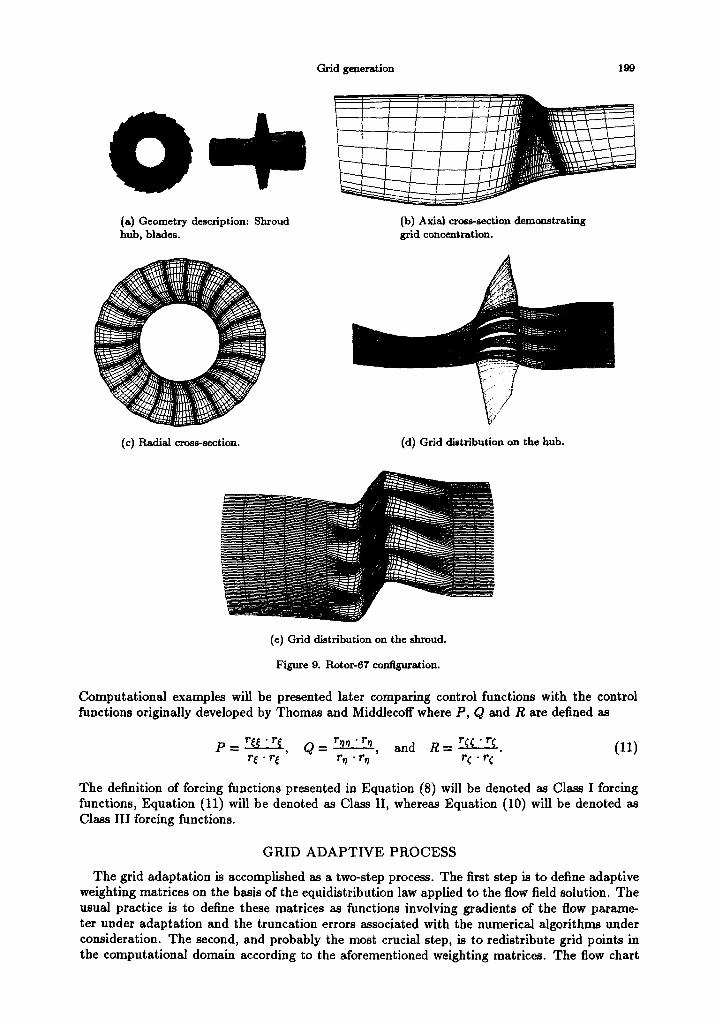
The final example represents the internal flow configuration involving rotor-67 geometry. In this example, shroud (Figures 9a-e) is treated as the outer boundary. The axial and radial cross- sections are presented in Figures 9b-c. Figures 9d-e demonstrate the grid concentration on hub and shroud as well as application of Bezier curves in resolving slope continuities. Observe the Bezier curves between blade tips projected on the shroud surface (Figure 9e). Well-distributed smooth and near orthogonal grids presented in Figures 9b-e demonstrate the success of the presented methodologies.

REFERENCES

1. J.F. Thomlmon, Program EAGLE: Numerical grid generation system user's manual, Vols. II and IH, AFATL-TR-15, (1987).

2. J.F. Thoml~on and B. Gatlin, Eas~ EAGLE: An Introduction to the EAGLE Grid Code, Mi~uippi State University, (1988).

3. J.F. Thompuon, A General three-dimensional elliptic grid generation system on a compodte block structure, Computer Me~hod~ in Applied Mech=nieJ and Enoineering (1987).

4. B.K. Soni, GENIE: GENeration d computational geometry-grids for internal-external flow configtwatious, Proceedings o] the N*tmerical Grid Generation in Computational Fhtid Mechanics '88, ~mnd, Fl~tda, (1988).

5. B.K. Soni, M.D. McClure and C.W. MMtin, Geometry and ~e~eration in N + 1 easy stepa, TI~e First l*t~erna~ional Conference on N~merical Grid Generation in Compntaiional FIttid DTnaraies, Lanchthut, W. GermAny, (1986).

Grid generation 201

6. B.K. Soul, Two- and three-dlmensional grid generation for internal flow applications of computational fluid dynamics, AIAA-1526-85.

7. J. Steinbrenner and C. Foits, GRIDGEN: User's Manual, Wright Research and Development Center and General Dynamics, Fort Worth Division, (1990).

8. R.L. Sorenson, Three-dimensiorud zonal grids about arbitrary shapes by Poisson's equation, Numerical Grid Generation in Computational Fluid Mechanics '88, Pineridge Press.

9. P.R. Elseman, Grid generation for fluid mechanics computations, Annual Review Fluid Mechanics (1985). 10. J.L. Steger and D.S. Chauseee, Generation of body-fitted coordinates using hyperbolic partial differential

equations, SIAM Journal of Scientific Statistic Computation (1980). 11. J. Thompson, Editor, Numerical Grid Generation, Elsevier Science Publishing Co., (1982). 12. B.K. Soul and M.-H. Shih, TURBOGRID: Turbomachinery applications of grid genecation, AIAA-90-2242,

~6 th AIAA/SAE/ASME/ASEE Joint Propulsion Con/erence, (1990). 13. T.-S. Wang and B.K. Soni, Goodness-of-grid: Quantitative measures, First Computational Fluid Dynamic

Congress (July 1988). 14. C.W. Mastin, B.K. Sold and M.D. McClure, Experience in grid optimization, AIAA-87-0201, Reno, NV,

(January 1987). 15. W. Schmldt, Strategies in mesh generation based on industrial requirements, First International Conference

on Numerical Grid Generation in Computational Fluid Dynamics, Landshut, W. GermAny, (July 1986). 16. P.R. Elseman, Lecture Notes in Ph~lsies, Series 141, Presented at the ?oh International Conference on

Numerical Methods in Fluid D~namics, Stanford, CA, (1980). 17. P.R. Eiseman, Geometric methods in computational fluid dynamics, ICASE-80-11, NASA Langley Research

Center, (1980). 18. C.R. Forsey, M.G. Edwards and M.P. Carr, An investigation of grid patching tecbnique, NASA Conference

Publication 2166, (WNGG)-NASA, (1980). 19. J.F. Middlecoff and P.D. Thomas, Direct control of the grid point distribution in meshes generated by elliptic

equations, AIAA-79-1462~ Presented at the AIAA 4th Computational D~namies Conference, Willlamsburg, VA, (1979).