Ground-states for the liquid dropand TFDW models with long-rangeattraction Cite as: J. Math. Phys. 58, 103503 (2017); https://doi.org/10.1063/1.4999495Submitted: 08 August 2017 . Accepted: 20 September 2017 . Published Online: 06 October2017
Stan Alama, Lia Bronsard, Rustum Choksi, and Ihsan Topaloglu
COLLECTIONS
This paper was selected as Featured
ARTICLES YOU MAY BE INTERESTED IN
Discrete diffraction managed solitons: Threshold phenomena and rapid decay forgeneral nonlinearitiesJournal of Mathematical Physics 58, 101513 (2017); https://doi.org/10.1063/1.5004253
Extended symmetry analysis of generalized Burgers equationsJournal of Mathematical Physics 58, 101501 (2017); https://doi.org/10.1063/1.5004134
Sasakian manifolds with purely transversal Bach tensorJournal of Mathematical Physics 58, 103502 (2017); https://doi.org/10.1063/1.4986492
Ground-states for the liquid drop and TFDW modelswith long-range attraction
Stan Alama,1,a) Lia Bronsard,1,b) Rustum Choksi,2,c) and Ihsan Topaloglu3,d)1Department of Mathematics and Statistics, McMaster University, Hamilton,Ontario L8S 4K1, Canada2Department of Mathematics and Statistics, McGill University, Montreal,Quebec H3A 0B9, Canada3Department of Mathematics and Applied Mathematics, Virginia Commonwealth University,Richmond, Virginia 23284, USA
(Received 8 August 2017; accepted 20 September 2017; published online 6 October 2017)
We prove that both the liquid drop model in R3 with an attractive background nucleusand the Thomas-Fermi-Dirac-von Weizsacker (TFDW) model attain their ground-states for all masses as long as the external potential V (x) in these models is oflong range, that is, it decays slower than Newtonian (e.g., V (x) |x |−1 for large |x|.)For the TFDW model, we adapt classical concentration-compactness arguments byLions, whereas for the liquid drop model with background attraction, we utilize arecent compactness result for sets of finite perimeter by Frank and Lieb. Published byAIP Publishing. https://doi.org/10.1063/1.4999495
I. INTRODUCTION
In this note, we consider ground-states of two mass-constrained variational problems containingan external attractive potential to the origin which is super-Newtonian at long ranges. The first problemconsists of a variant of Gamow’s liquid drop problem1–3 perturbed by an attractive backgroundpotential V (x), with long range decay, in the sense that V (x) |x |−1 for large |x|. The second problemis a variant of the Thomas-Fermi-Dirac-von Weizsacker (TFDW) functional, again subject to anexternal attractive potential V (x) which is “super-Newtonian.”
Let us first state the two problems precisely. The variant of the liquid drop problem is givenby
eV (M) B inf
EV (u) : u ∈ BV (R3; 0, 1),
∫R3
u dx =M
, (LD)
where the energy functional EV is defined as
EV (u)B∫R3|∇u| +
∫R3
∫R3
u(x)u(y)|x − y|
dxdy −∫R3
V (x)u(x) dx. (1)
Here the first term in EV computes the total variation of the function u, i.e.,∫R3|∇u| = sup
∫R3
u div φ dx : φ ∈C10 (R3;R3), |φ| 6 1
and is equal to PerR3 (x ∈R3 : u(x)= 1) since u takes on only the values 0 and 1.
The variant of the TFDW problem we consider here is to find
103503-2 Alama et al. J. Math. Phys. 58, 103503 (2017)
where
EV (u)B∫R3
(|∇u|2 + |u|10/3 − |u|8/3 − V (x)|u|2
)dx +
12
∫R3
∫R3
|u(x)|2 |u(y)|2
|x − y|dxdy. (2)
In the original TFDW problem (see the works of Benguria, Brezis, Lieb,4 Le Bris, Lions,5 andLieb6 for detailed surveys on this classical theory), the potential is taken to be
VZ (x)BZ|x |
,
simulating an attracting point charge at the origin with charge Z. With this physical choice of potential,both the liquid drop and TFDW problems have been shown to exhibit existence for small M andnonexistence for large M. In particular, for the liquid drop model, it has recently been shown by Luand Otto, and by Frank, Nam, and van den Bosch that
(nonexistence, Theorem 1.4 of Frank, Nam, and van den Bosch7) if EVZ has a minimizer, thenM 6min2Z + 8, Z + CZ1/3 + 8 for some C > 0; and
(existence, Theorem 2 of Lu and Otto8) there exists a constant c > 0 so that for M 6 Z + c, theunique minimizer of EVZ is given by the ball χB(0,R),
where R = (M/ω3)1/3 and ω3 denotes the volume of the unit ball in R3. Similar (and older) existenceresults hold for the TFDW problem. The existence of solutions to the classical TFDW problem wasestablished by Lions9 for M 6 Z and extended to M 6 Z + c for some constant c > 0 by Le Bris.10 Thenonexistence of ground-states for large values of M (or small values of Z) is only recently provedby Frank, Nam, and van den Bosch.7,11 In a separate paper, Nam and van den Bosch11 also considermore general external potentials which are short-ranged, i.e., lim |x |→∞ |x |V (x)= 0. Motivated bytheir result, here we look at the complementary case, in which the external potential is asymptoticallylarger than Newtonian at infinity.
These functionals can be viewed as mathematical paradigms for the existence and nonexistenceof coherent structures based upon a mass parameter. Since both problems are driven by a repulsivepotential of Coulombic (Newtonian) type, it is natural to expect that if the confining external potentialV was even slightly stronger (at long ranges) than Newtonian, global existence would be restored forall masses. In this note, we prove that this is indeed the case.
For the liquid drop problem eV , we consider the external potentials V which satisfy the followinghypotheses:
(H1) V > 0 and V ∈ L1loc(R3).
(H2) limt→∞
t
(inf|x |=t
V (x)
)=∞.
(H3) lim|x |→∞
V (x)= 0.
On the other hand, to ensure that the energy EV is bounded below, we assume that V satisfies
(H1′) V > 0 and V ∈ L3/2(R3) + L∞(R3),
instead of (H1), along with (H2) and (H3). Hypothesis (H2) implies that these potentials are long-ranged but only slightly more attractive than Newtonian. A typical example of such an externalpotential is
V (x)=1
|x |1−ε
for 0 < ε < 1 or a linear combination of functions of this form. Although these potentials have onlyslightly longer range than |x|1, this is sufficient to ensure the existence of ground-states for themodified liquid drop and TFDW problems, eV and IV , for all M > 0.
Theorem 1 (Liquid drop model). Suppose V satisfies (H1)–(H3), then for any M > 0, the problemeV (M) given by (LD) has a solution.
103503-3 Alama et al. J. Math. Phys. 58, 103503 (2017)
Theorem 2 (TFDW model). Suppose V satisfies (H1′), (H2), and (H3), then for any M > 0, theproblem IV (M) given by (TFDW) has a solution.
Remark 3. While we do obtain the existence of ground-states for all masses M, we do not expectthat the attractive potential V stabilizes the single droplet solution χB(0,(M/ω3))1/3 for large values ofM. Rather, we expect that mass splitting does indeed occur (as it does for the unperturbed liquid dropproblem3,12,13), but the resulting components are confined by the external potential V and cannotescape to infinity. This expectation is reflected in our approach to the proof of the two theoremsabove.
While the mathematical motivations for these results are clear, let us now comment on thephysicality of the long-range super-Newtonian attraction. For the quantum TFDW model, we donot know of any physical situation which would support an “exterior” potential producing super-Newtonian attraction. However we note that these functionals, in particular, the liquid drop energy,can be used as phenomenological models for charged or gravitating masses at all length scales.Consideration of super-Newtonian forces appears in several theories at the cosmological level, andin fact, the validity of Newton’s law at long distances has been a longstanding interest in physics.As Finzi notes,14 for example, stability of cluster of galaxies implies stronger attractive forces atlong distances than that predicted by Newton’s law. Motivated by similar observations, Milgrom15
introduced the modified Newtonian dynamics (MOND) theory which suggests that the gravitationalforce experienced by a star in the outer regions of a galaxy must be stronger than Newton’s law (seealso works of Bugg16 and Milgrom17 for a survey, and Bekenstein’s work18).
A. Outline of the paper
The proofs of Theorems 1 and 2 follow the same basic strategy: to obtain a contradiction, weassume that minimizing sequences lose compactness, and use concentration compactness techniquesto show that it is because of the splitting and dispersion of mass to infinity (“dichotomy”). For theliquid drop model, we utilize a recent technical concentration-compactness result for sets of finiteperimeter by Frank and Lieb19 to prove a lower bound on the energy in case minimizing sequencesun lose compactness via splitting of the form
limn→∞
EV (un) > eV (m0) + e0(m1) + e0(M − m0 − m1), (3)
where 0 <mi <M with m0 + m1 6M. However, thanks to the super-Newtonian decay of V, wethen show that eV (M) actually lies strictly below the value given in (3). This is a variant on theoriginal “strict subadditivity” argument introduced by Lions9 for the classical TFDW model withV (x) = |x|1 and subsequently used in innumerable treatments of variational problems with loss ofcompactness.
In Sec. III, we adapt recent arguments by Nam and van den Bosch11 along with estimates ofLions9 and Le Bris10 to prove Theorem 2. Although the variational structure of TFDW is nearlythe same as the liquid drop model, the components are not compactly supported, so we require anadditional argument to verify that they decay sufficiently rapidly (in fact exponentially) in order tocalculate the interaction between components.
II. PROOF OF THEOREM 1
Our proof relies on a recent concentration-compactness type result for sets of finite perimeterby Frank and Lieb.19 While similar compactness results are known and could be adapted here (forexample, the classical theory of Lions,20 and results for minimizing clusters which can be found inChap. 29 of Maggi21), the results of Frank and Lieb are particularly well-suited for our purposes.Throughout the proof of Theorem 1, we specifically use Proposition 2.1 and Lemmas 2.2 and 2.3 ofFrank and Lieb.19
103503-4 Alama et al. J. Math. Phys. 58, 103503 (2017)
As noted in the Introduction, our goal is to obtain a splitting property (3) for eV (M) involvingthe “minimization problem at infinity” e0 given by
e0(M) B inf
E0(u) : u ∈ BV (R3; 0, 1), and
∫R3
u dx =M
,
where
E0(u) B∫R3|∇u| +
∫R3
∫R3
u(x)u(y)|x − y|
dxdy.
We will also use the following simple weak compactness result for the confinement term, whichis convenient to state in general terms.
Lemma 4. Let An ⊂R3 be a sequence of sets with |An | 6M which converge to zero locally, i.e.,χAn→ 0 in L1
loc(R3). Then ∫An
V dx =∫R3
V χAn dx→ 0 as n→∞.
Proof. By hypothesis (H3), for any ε > 0, there exists R > 0 so that if V∞BV χBcR, then
0 6 V∞ < ε3M . By (H1), on the other hand, we define V1BV χBR\EK , where EK = x ∈ BR : 0 6 V (x)
6K and K is chosen with ‖V1‖L1(R3) <ε3 . Finally, let V2BV χEK , which is supported in BR, and
satisfies ‖V2‖L∞(R3) 6K .Now with these choices, we have a decomposition of V into V1 + V2 + V∞, depending on ε and
K. Using this decomposition
0 6∫
An
V dx 6 ‖V1‖L1 + K |An ∩ BR | +ε
3M|An | <K |An ∩ BR | +
2ε3< ε ,
for all n large enough, since |An ∩ BR | → 0 as n→∞ by local convergence of the sets An.
Proof of Theorem 1. First, by (H1) and (H3), we may write V =V χBR + V χBcR∈ L1 + L∞, where
R is chosen so that ‖V χBcR‖L∞(R3) 6 1. Then, for any u= χΩ with |Ω| =M,∫
R3Vu dx 6 ‖V ‖L1(BR) + M,
hence, eV (M)>−∞. Now, let unn∈N ⊂ BV (R3; 0, 1) with∫R3
un dx =M be a minimizing sequence
for the energy EV , i.e., limn→∞ EV (un)= eV (M). By the above estimate on the confinement term, theminimizing sequence has uniformly bounded perimeter, ∫R3 |∇un | 6C independent of n. Define thesets of finite perimeter Ωn ⊂R3 so that χΩn = un, and |Ωn | =M for all n ∈N.
Step 1. First, we set up our contradiction argument. By the compact embedding of BV (R3)in L1
loc(R3) (see, e.g., Corollary 12.27 in Maggi21), there exists a subsequence and a set of finiteperimeter Ω0 ⊂R3 so that Ωn→Ω
0 locally, that is, un→ χΩ0 B w0 in L1loc(R3). At this point, we
admit the possibility that w0 ≡ 0, i.e., |Ω0 | = 0. However, in Step 4, we show that w0 . 0.If the limit set |Ω0 | =M, then we are done. Indeed, since unn∈N is locally convergent in L1,
a subsequence converges almost everywhere in R3. In addition, the norms converge, ‖un‖L1 =M= ‖ χΩ0 ‖L1 , so by the Brezis-Lieb Lemma (see Theorem 1.9 in Lieb and Loss22), we may thenconclude that (along a subsequence) un→ w0 = χΩ0 in L1 norm. By the lower semicontinuity of theperimeter (Proposition 4.29 in Maggi21) and of the interaction terms (Lemma 2.3 of Frank and Lieb19)∫
R3|∇w0 | 6 lim inf
n→∞
∫R3|∇un |
∫R3
∫R3
w0(x)w0(y)|x − y|
dxdy 6 lim infn→∞
∫R3
∫R3
un(x)un(y)|x − y|
dxdy.
To pass to the limit in the confinement term, we apply Lemma 4 to the sequence un − w0→ 0 in
L1(R3), and together with the above, we have
EV (w0) 6 lim infn→∞
EV (un).
103503-5 Alama et al. J. Math. Phys. 58, 103503 (2017)
Therefore we conclude that w0 = χΩ0 attains the minimum value of EV , and the proof is complete.To derive a contradiction, we now assume that m0B |Ω
0 | <M.
Step 2. Next, we show that the energy splits. First, assume that 0 < |Ω0 | <M. We apply Lemma2.2 of Frank and Lieb19 (with xn = x0
n = 0): there exists rn > 0 such that the sets
U 0n =Ωn ∩ Brn and V 0
n =Ωn ∩ (R3 \ Brn )
satisfy
χU0n→ χΩ0 in L1(R3), χV0
n→ 0 in L1
loc(R3),
limn→∞|U0
n | = |Ω0 | =m0, PerΩ0 6 lim inf
n→∞Per U 0
n ,
and limn→∞
(PerΩn − Per U 0n − Per V0
n)= 0.
We now define w0n (x)B χU0
n(x), w0(x)B χΩ0 (x), Ω0
nBV0n, and u0
n(x)B χΩ0n(x) so that un = w
0n
+ u0n = w
0 + u0n + o(1) in L1(R3), and u0
n→ 0 in L1loc. In particular, by Lemma 4,∫
R3Vun dx =
∫R3
Vw0 dx + o(1).
Using Lemma 2.3 in the work by Frank and Lieb,19 the nonlocal interaction term in EV splits in asimilar way as the perimeter,∫
R3
∫R3
un(x) un(y)|x − y|
dxdy=∫R3
∫R3
w0n (x) w0
n (y)|x − y|
dxdy +∫R3
∫R3
u0n(x) u0
n(y)|x − y|
dxdy + o(1)
=
∫R3
∫R3
w0(x) w0(y)|x − y|
dxdy +∫R3
∫R3
u0n(x) u0
n(y)|x − y|
dxdy + o(1),
and thus the energy splits, up to a small error,
EV (un)=EV (w0n ) + E0(u0
n) + o(1) >EV (w0) + E0(u0n) + o(1). (4)
In the case |Ω0 | = 0 (which we eliminate in Step 4 below), this splitting becomes trivial, withw0 ≡ 0 and u0
n = un.
Step 3. Now we repeat the above procedure to locate a concentration set for the remainder u0n.
We argue as above, but with u0n replacing un, that is, the remainder set Ω0
n =V0n replacing Ωn. We
know that u0n = χΩ0
n→ 0 locally in L1(R3), |Ω0
n | =M − m0 + o(1) ∈ (0, M], and EV (u0n) (and hence
PerΩ0n) are uniformly bounded. By Proposition 2.1 in the work by Frank and Lieb,19 there exists a
setΩ1 with 0 < |Ω1 | 6M −m0 and a sequence of translations xn ∈R3 such that for some subsequenceχΩ0
n−xn→ χΩ1 in L1
loc(R3). Since χΩ0n→ 0 L1
loc(R3), we have that the translation points |xn | →∞ as
n→∞. Again, by Lemmas 2.2 and 2.3 of Frank and Lieb,19 and Lemma 4 as in Step 2, we similarlyobtain a disjoint decomposition Ω0
n − xn =U1n ∪ V1
n, with χU1n→ χΩ1 in L1(R3), χV1
n→ 0 in L1
loc(R3),and for which the energy splits as in (4), namely,
EV (u0n)=E0(u0
n) + o(1) >E0(w1) + E0(u1n) + o(1),
where w1B χΩ1 , u1n = χV1
n+xn→ 0 in L1
loc(R3), and |V1n | = |V0
n | −m1 + o(1). We denote the re-centered
remainder set Ω1nBV1
n + xn so that u1n(x)= χΩ1
n(x). Combining with the previous step, we now have
EV (un) >EV (w0) + E0(w1) + E0(u1n) + o(1) and M =m0 + m1 + |Ω1
n | + o(1).
This, combined with the continuity of e0 (see, e.g., Lemma 4.8 in the work of Knupfer, Muratov, andNovaga13) yields a lower bound estimate in case of splitting,
eV (M) > eV (m0) + e0(m1) + e0(M − m0 − m1). (5)
Step 4. We claim that w0 . 0. For a contradiction, assume w0 ≡ 0. Define a sequence by wn(x)B un(x + xn) using the translation sequence found above. Then wn→ w1 in L1(R3) and wn − u0
n→ 0
103503-6 Alama et al. J. Math. Phys. 58, 103503 (2017)
in L1loc(R3). This implies, by Lemma 4, that limn→∞ ∫R3 V (wn − u0
n) dx = 0. Now this limit and thetranslation invariance of the first two terms of EV yield
EV (wn) − EV (un)=−∫R3
V (wn − un) dx −→−∫R3
Vw1dx < 0,
hence, a contradiction.
Step 5. Now we prove that eV (m0)=EV (w0) and e0(m1)=E0(w1). By subadditivity (see Lemma4 of Lu and Otto8 and Lemma 3 in their earlier work,12 or Step 5 below), we have a rough upperbound estimate of the form
eV (M) 6 eV (m0) + e0(m1) + e0(M − m0 − m1).
Combined with (5), this yields
eV (m0) + e0(m1) + e0(M − m0 − m1) > eV (M)
>EV (w0) + E0(w1) + lim infn→∞
E0(u1n)
> eV (m0) + e0(m1) + e0(M − m0 − m1).
Hence, (EV (w0) − eV (m0))
+(EV (w1) − eV (m1)
)+
(lim inf
n→∞E0(u1
n) − e0(M − m0 − m1))= 0,
and since every term in this sum are nonnegative, we must conclude that
EV (w0)= eV (m0) and E0(w1)= e0(m1).
Step 6. Finally, we show, by means of an improved upper bound, that splitting leads to a con-tradiction, and hence the minimum must be attained. It is here that we use the super-Newtonianattraction hypothesis (H2). Since w0 = χΩ0 (x), w1 = χΩ1 (x) are minimizers of eV and e0 respectively,by regularity of minimizers,3,8 we may choose R > 0 for which Ω0, Ω1 ⊂ BR(0). Let b ∈ S2 be anyunit vector. For t sufficiently large so that Ω0 ∩ (Ω1 + tb)= ∅, let
F(t)B∫R3
∫R3
w0(x)w1(y − tb)4π |x − y|
dxdy, and G(t)B∫R3
V (x)w1(x − tb) dx.
We now estimate each; first,
F(t) 6∫
BR(0)
∫BR(tb)
14π |x − y|
dx dy 6|BR |
2
4π(t − 2R)6|BR |
2
2πt,
for all t large enough.To estimate G(t) from below, we recall from (H2) that for any A> 0, there exists t1 > 0 such that
for all t > t1,
inf|x |=t
V (x) >At
.
Thus, for each i= 1, . . . , N , as t→∞,
t∫R3
V (x)w1(x − tb) dx =∫Ω1
tV (x + tb) dx >∫Ω1
tA|x + tb|
dx −→A|Ω1 |,
by dominated convergence, and hence limt→∞ tG(t)=∞. Thus, t(F(t)−G(t))→−∞ as t→∞. Chooseε > 0 and t0 > 0 such that
F(t0) − G(t0)<−ε < 0.
With this choice of ε > 0, we may choose a compact set K =K(ε) for which |K | = M m0 m1
andE0(χK )< e0(M − m0 − m1) +
ε
3.
Choose τ > 0 large enough so that Kτ BK − τb satisfies∫Ωi
∫Kτ
14π |x − y|
dx dy <ε
3, for i= 0, 1.
103503-7 Alama et al. J. Math. Phys. 58, 103503 (2017)
Using v(x)= w0(x) + w1(x − t0b) + χKτ as a test function, which is admissible for eV (M), we have
which contradicts the lower bound in case of splitting, (5). Thus we must have |Ω0 | =M and eV (M)=EV (w0), for any M > 0.
III. PROOF OF THEOREM 2
Now we turn our attention to EV and IV (M) given by (2) and (TFDW), respectively. As in Sec. II,we define the “problem at infinity” by
I0(M) B inf
E0(u) : u ∈H1(R3),
∫R3|u|2 dx =M
,
where
E0(u)B∫R3
(|∇u|2 + |u|10/3 − |u|8/3
)dx +
12
∫R3
∫R3
|u(x)|2 |u(y)|2
|x − y|dxdy.
First we note that problems IV and I0 satisfy the following “binding inequality,” which is thestandard subadditivity condition from concentration-compactness principle. For the proof of thefollowing lemma, we refer to Lemma 5 in Nam and van den Bosch.11
Lemma 5. For all 0 <m <M, we have that
IV (M) 6 IV (m) + I0(M − m).
Moreover, IV (M)< I0(M)< 0, IV (M) is continuous and strictly decreasing in M.
Next we prove that the ground-state value IV (M) is bounded.
Lemma 6. Let unn∈N ⊂H1(R3) be a minimizing sequence for the energy EV with ∫R3 |un |2 dx
=M. Then there exists constant C0 > 0 such that ‖un‖2H1(R3)
6C0 M.
Proof. First, we note that IV (M)< 0 for any M > 0. Indeed, in the proof Lemma 5 of Namand van den Bosch,11 it is shown that I0(M)< 0, and EV (u) 6 E0(u) holds for all u ∈H1(R3) with∫R3 |u|2 dx =M. We first claim that the quadratic form defined by the Schrodinger operator ∆ V (x)is bounded below, i.e., that there exists λ > 0 with∫
R3
(|∇u|2 − V (x)|u|2
)dx >
12‖u‖2H1 − λ‖u‖
2L2 ,
for all u ∈H1(R3). To see this, we note that by (H1′), we may write V = V1 + V2 with V1 ∈ L3/2(R3)and V2 ∈ L∞(R3). Moreover, we may assume that ‖V1‖L3/2(R3) < ε for some ε > 0 to be chosen later.By the Holder and Sobolev inequalities, it follows that∫
R3|V1 | |u|
2 dx 6 ‖V1‖L3/2(R3)‖u‖2L6(R3)
6 ε S3 ‖∇u‖2L2(R3)
,
where S3 > 0 is the Sobolev constant. Thus,∫R3
(|∇u|2 − V (x)|u|2
)dx > (1 − ε S3)‖∇u‖2
L2(R3)− ‖V2‖L∞(R3)‖u‖
2L2(R3)
,
and the lower bound is obtained by choosing
ε =1
2S3and λ = ‖V2‖L∞(R3) +
12
.
103503-8 Alama et al. J. Math. Phys. 58, 103503 (2017)
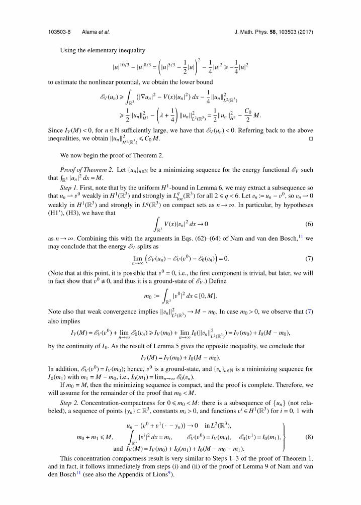
Using the elementary inequality
|u|10/3 − |u|8/3 =
(|u|5/3 −
12|u|
)2
−14|u|2 > −
14|u|2
to estimate the nonlinear potential, we obtain the lower bound
EV (un) >∫R3
(|∇un |
2 − V (x)|un |2) dx −
14‖un‖
2L2(R3)
>12‖un‖
2H1 −
(λ +
14
)‖un‖
2L2(R3)
=12‖un‖
2H1 −
C0
2M.
Since IV (M)< 0, for n ∈N sufficiently large, we have that EV (un)< 0. Referring back to the aboveinequalities, we obtain ‖un‖
2H1(R3)
6C0 M.
We now begin the proof of Theorem 2.
Proof of Theorem 2. Let unn∈N be a minimizing sequence for the energy functional EV suchthat ∫R3 |un |
2 dx =M.
Step 1. First, note that by the uniform H1-bound in Lemma 6, we may extract a subsequence sothat un v0 weakly in H1(R3) and strongly in Lq
loc(R3) for all 2 6 q < 6. Let vnB un − v0, so vn 0
weakly in H1(R3) and strongly in Lq(R3) on compact sets as n→∞. In particular, by hypotheses(H1′), (H3), we have that ∫
R3V (x)|vn |
2 dx→ 0 (6)
as n→∞. Combining this with the arguments in Eqs. (62)–(64) of Nam and van den Bosch,11 wemay conclude that the energy EV splits as
limn→∞
(EV (un) − EV (v0) − E0(vn)
)= 0. (7)
(Note that at this point, it is possible that v0 = 0, i.e., the first component is trivial, but later, we willin fact show that v0 . 0, and thus it is a ground-state of EV .) Define
m0 B
∫R3|v0 |2 dx ∈ [0, M].
Note also that weak convergence implies ‖vn‖2L2(R3)
→M − m0. In case m0 > 0, we observe that (7)
also implies
IV (M)=EV (v0) + limn→∞
E0(vn) > IV (m0) + limn→∞
I0(‖vn‖2L2(R3)
)= IV (m0) + I0(M − m0),
by the continuity of I0. As the result of Lemma 5 gives the opposite inequality, we conclude that
IV (M)= IV (m0) + I0(M − m0).
In addition, EV (v0)= IV (m0); hence, v0 is a ground-state, and vnn∈N is a minimizing sequence forI0(m1) with m1 = M m0, i.e., I0(m1)= limn→∞ E0(vn).
If m0 = M, then the minimizing sequence is compact, and the proof is complete. Therefore, wewill assume for the remainder of the proof that m0 <M.
Step 2. Concentration-compactness for 0 6m0 <M: there is a subsequence of un (not rela-beled), a sequence of points yn ⊂R3, constants mi > 0, and functions v i ∈H1(R3) for i = 0, 1 with
un −(v0 + v1( · − yn)
)→ 0 in L2(R3),
m0 + m1 6M,∫R3|v i |2 dx =mi, EV (v0)= IV (m0), E0(v1)= I0(m1),
and IV (M)= IV (m0) + I0(m1) + I0(M − m0 − m1).
(8)
This concentration-compactness result is very similar to Steps 1–3 of the proof of Theorem 1,and in fact, it follows immediately from steps (i) and (ii) of the proof of Lemma 9 of Nam and vanden Bosch11 (see also the Appendix of Lions9).
103503-9 Alama et al. J. Math. Phys. 58, 103503 (2017)
Step 3. Next, we claim that v0 . 0. This follows by the same arguments as in Step 4 of the proofof Theorem 1. Indeed, assume the contrary, so m0 = 0. Then by Lemma 5 and (8), we would have
IV (M) 6 I0(M) 6 I0(m1) + I0(M − m1)= IV (M),
and so IV (M) = I0(M). But the energy functional E0 is translation invariant; hence, we may pull backthe component, un(x)B un(x + yn) with the same E0 value, and obtain
IV (M)= I0(M)= limn→∞
E0 (un)= limn→∞
[EV (un) +
∫R3
V (x) |un |2 dx
]
> IV (M) + lim infn→∞
∫R3
V (x) |un |2 dx = IV (M) +
∫R3
V (x)|v1 |2 dx
> IV (M),
a contradiction. Therefore m0 > 0 and v0 is a nontrivial ground-state of IV (m0).
Step 4. Both v0 and v1 are strictly positive and have exponential decay, i.e., 0 < v i(x) 6Ce−ν |x | ,for constants C, ν > 0 and for i = 0, 1. To show this, we first follow the Appendix in Lions9 and notethat, by Ekeland’s variational principle,23 we may find a minimizing sequence un for IV (M), with
‖un − un‖H1(R3)→ 0 (9)
and which approximately solve the Euler-Lagrange equations, ‖DEV (un)− µnun‖H−1(R3)→ 0, that is,
−∆un +[f (un) − V (x)(|un |
2 ∗ |x |−1) − µn
]un −→ 0,
in H−1(R3), with f (t)= 53 t4/3− 4
3 t2/3, and Lagrange multiplier µn. As ‖un‖H1(R3) is uniformly bounded,using un as a test function, we readily show that the Lagrange multipliers µn are bounded, andpassing to a limit along a subsequence, µn→ µ. Furthermore, by Step 2 and (9), un admits the samedecomposition (8) into components v i as does un, and using weak convergence, we obtain a limitingPDE for each component,
−∆v0 +[f (v0) − V (x) +
((v0)2 ∗ |x |−1
)]v0 = µv0,
−∆v1 +[f (v1) +
((v1)2 ∗ |x |−1
)]v1 = µv1,
with the same Lagrange multiplier µ. By minimization, v i > 0 and by the strong maximum principle,we may conclude that each v i > 0 for i = 0, 1.
Next, we show that the Lagrange multiplier µ < 0. Following the proof of Theorem 1 of Le Bris,10
we define the spherical mean of an integrable ψ as ψ(x)= 14π ∫σ∈S2 ψ(|x |σ) dS(σ), and note that by
Newton’s Theorem (see Theorem 9.7 of Lieb and Loss22),
(v0)2 ∗ |x |−1 = (v0)2 ∗ |x |−1 6 |x |−1∫R3
(v0)2 dx 6M|x |
.
By (H2), there exists R > 0 for which V (x) > M|x | for all |x | > R, and hence
(v0)2 ∗ |x |−1 − V 6 0 for all |x | > R. (10)
Assume for a contradiction that µ> 0. Set W B 53 |v
0 |4/3 + [(v0)2 ∗ |x |−1] − V , so v0 satisfies thedifferential inequality,
−∆v0 + W v0 =
(23
(v0)5/3 + µ
)v0 > 0
in R3. By (10), outside BR, W+ =53 (v0)4/3 ∈ L3/2. Applying Theorem 7.18 of Lieb,6 we conclude that
v0 <L2(BcR), a contradiction. Thus, µ < 0.
Finally, from Eq. (66) of Lions,9 we may conclude that the solutions are exponentially localized,
|∇v i(x)| + |v i(x)| 6Ce−ν |x | (11)
for i = 0, 1 with 0 < ν <√−µ.
103503-10 Alama et al. J. Math. Phys. 58, 103503 (2017)
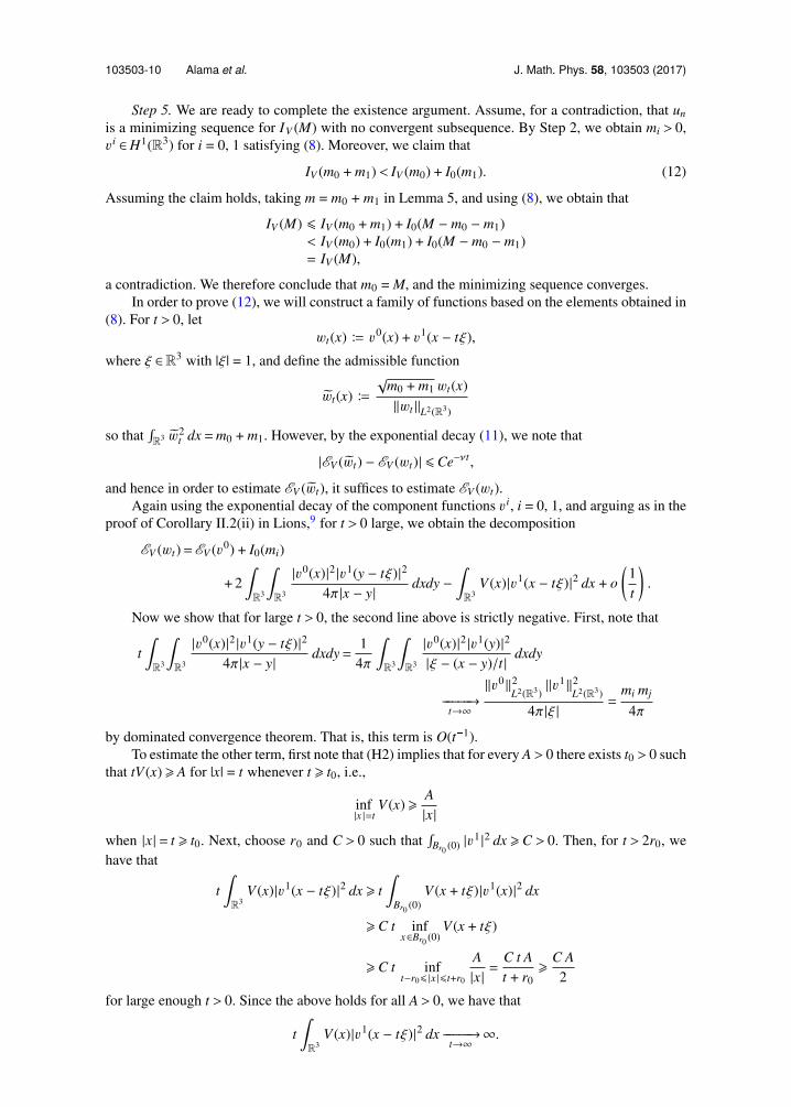
Step 5. We are ready to complete the existence argument. Assume, for a contradiction, that un
is a minimizing sequence for IV (M) with no convergent subsequence. By Step 2, we obtain mi > 0,v i ∈H1(R3) for i = 0, 1 satisfying (8). Moreover, we claim that
IV (m0 + m1)< IV (m0) + I0(m1). (12)
Assuming the claim holds, taking m = m0 + m1 in Lemma 5, and using (8), we obtain that
IV (M) 6 IV (m0 + m1) + I0(M − m0 − m1)< IV (m0) + I0(m1) + I0(M − m0 − m1)= IV (M),
a contradiction. We therefore conclude that m0 = M, and the minimizing sequence converges.In order to prove (12), we will construct a family of functions based on the elements obtained in
(8). For t > 0, letwt(x) B v0(x) + v1(x − tξ),
where ξ ∈R3 with |ξ | = 1, and define the admissible function
wt(x) B
√m0 + m1 wt(x)
‖wt ‖L2(R3)
so that ∫R3 w2t dx =m0 + m1. However, by the exponential decay (11), we note that
|EV (wt) − EV (wt)| 6Ce−νt ,
and hence in order to estimate EV (wt), it suffices to estimate EV (wt).Again using the exponential decay of the component functions v i, i = 0, 1, and arguing as in the
proof of Corollary II.2(ii) in Lions,9 for t > 0 large, we obtain the decomposition
EV (wt)=EV (v0) + I0(mi)
+ 2∫R3
∫R3
|v0(x)|2 |v1(y − tξ)|2
4π |x − y|dxdy −
∫R3
V (x)|v1(x − tξ)|2 dx + o
(1t
).
Now we show that for large t > 0, the second line above is strictly negative. First, note that
t∫R3
∫R3
|v0(x)|2 |v1(y − tξ)|2
4π |x − y|dxdy=
14π
∫R3
∫R3
|v0(x)|2 |v1(y)|2
|ξ − (x − y)/t |dxdy
−−−−−→t→∞
‖v0‖2L2(R3)
‖v1‖2L2(R3)
4π |ξ |=
mi mj
4π
by dominated convergence theorem. That is, this term is O(t1).To estimate the other term, first note that (H2) implies that for every A> 0 there exists t0 > 0 such
that tV (x) > A for |x| = t whenever t > t0, i.e.,
inf|x |=t
V (x) >A|x |
when |x | = t > t0. Next, choose r0 and C > 0 such that ∫Br0 (0) |v1 |2 dx >C > 0. Then, for t > 2r0, we
have that
t∫R3
V (x)|v1(x − tξ)|2 dx > t∫
Br0 (0)V (x + tξ)|v1(x)|2 dx
>C t infx∈Br0 (0)
V (x + tξ)
>C t inft−r06 |x |6t+r0
A|x |=
C t At + r0
>C A2
for large enough t > 0. Since the above holds for all A> 0, we have that
t∫R3
V (x)|v1(x − tξ)|2 dx −−−−−→t→∞
∞.
103503-11 Alama et al. J. Math. Phys. 58, 103503 (2017)
In particular, the confinement term dominates the other cross terms for t > 0 sufficiently large, andthus
IV (m0 + m1) 6 EV (wt)< IV (m0) + I0(m1),
proving our claim (12).
ACKNOWLEDGMENTS
The authors would like to thank the referees for their invaluable comments, which allowed usto simplify the proof of Theorem 2 significantly. S.A., L.B., and R.C. were supported by NSERC(Canada) Discovery Grants.
1 G. Gamow, “Mass defect curve and nuclear constitution,” Proc. R. Soc. A 126, 632–644 (1930).2 C. F. von Weizsacker, “Zur theorie der kernmassen,” Z. Phys. A 96, 431–458 (1935).3 H. Knupfer and C. B. Muratov, “On an isoperimetric problem with a competing nonlocal term II: The general case,”
Commun. Pure Appl. Math. 67, 1974–1994 (2014).4 R. Benguria, H. Brezis, and E. H. Lieb, “The Thomas-Fermi-von Weizsacker theory of atoms and molecules,” Commun.
Math. Phys. 79, 167–180 (1981).5 C. Le Bris and P.-L. Lions, “From atoms to crystals: A mathematical journey,” Bull. Am. Math. Soc. 42, 291–363 (2005).6 E. H. Lieb, “Thomas-Fermi and related theories of atoms and molecules,” Rev. Mod. Phys. 53, 603–641 (1981).7 R. L. Frank, P. T. Nam, and H. van den Bosch, “The ionization conjecture in Thomas-Fermi-Dirac-von Weizsacker theory,”
Comm. Pure Appl. Math. (to appear); preprint arXiv:1606.07355 (2016).8 J. Lu and F. Otto, “An isoperimetric problem with Coulomb repulsion and attraction to a background nucleus,” preprint
arXiv:1508.07172 (2015).9 P.-L. Lions, “Solutions of Hartree-Fock equations for Coulomb systems,” Commun. Math. Phys. 109, 33–97 (1987).
10 C. Le Bris, “Some results on the Thomas-Fermi-Dirac-von Weizsacker model,” Differ. Integr. Equations 6, 337–353 (1993),https://projecteuclid.org/euclid.die/1370870194.
11 P. T. Nam and H. van den Bosch, “Nonexistence in Thomas–Fermi–Dirac–von Weizsacker theory with small nuclearcharges,” Math. Phys. Anal. Geom. 20, 6 (2017).
12 J. Lu and F. Otto, “Nonexistence of a minimizer for Thomas-Fermi-Dirac-von Weizsacker model,” Commun. Pure Appl.Math. 67, 1605–1617 (2014).
13 H. Knupfer, C. B. Muratov, and M. Novaga, “Low density phases in a uniformly charged liquid,” Commun. Math. Phys.345, 141–183 (2016).
14 A. Finzi, “On the validity of Newton’s law at a long distance,” Mon. Not. R. Astron. Soc. 127, 21–30 (1963).15 M. Milgrom, “A modification of the Newtonian dynamics as a possible alternative to the hidden mass hypothesis,” Astrophys.
J. 270, 365–370 (1983).16 D. V. Bugg, “MOND—A review,” Can. J. Phys. 93, 119–125 (2015).17 M. Milgrom, “MOND theory,” Can. J. Phys. 93, 107–118 (2015).18 J. D. Bekenstein, “Relativistic gravitation theory for the modified Newtonian dynamics paradigm,” Phys. Rev. D 70, 083509
(2004).19 R. L. Frank and E. H. Lieb, “A compactness lemma and its application to the existence of minimizers for the liquid drop
model,” SIAM J. Math. Anal. 47, 4436–4450 (2015).20 P.-L. Lions, “The concentration-compactness principle in the calculus of variations. The locally compact case. I,” Ann. Inst.
Henri Poincare Anal. Non Lineaire 1, 109–145 (1984).21 F. Maggi, Sets of Finite Perimeter and Geometric Variational Problems, 1st ed., Cambridge Studies in Advanced Mathematics
Vol. 135 (Cambridge University Press, Cambridge, 2012).22 E. H. Lieb and M. Loss, Analysis, Graduate Studies in Mathematics Vol. 14 (American Mathematical Society, Providence,
RI, 1997), pp. xviii+278.23 I. Ekeland, “Nonconvex minimization problems,” Bull. Am. Math. Soc. 1, 443–474 (1979).