4.1. Different aspects of groundwater development in Odisha 8-40
4.1.1. Status of groundwater resources in Odisha 8-9
4.1.2. Groundwater irrigation-agricultural income linkage in Odisha 9
4.1.3. Factors affecting groundwater development in Odisha 10-11
4.1.4. Classification of districts using K-means clustering technique 11-13
4.1.5. Inter-cluster and intra-cluster variations in groundwater 14-15development
4.1.6. Inter-cluster and intra-cluster variations in groundwater table 15-18depth and aquifer properties
4.1.7. Temporal and spatial variations in groundwater structures and 18-21 ownership pattern
4.1.8. Inter-cluster variations in groundwater irrigation potential created 21-23(IPC) and its utilization (IPU)
4.1.9. Constraints in groundwater irrigation in Odisha 23-25
4.1.10. Energy use aspects of groundwater irrigation in Odisha 25-30
4.1.10.1. Major sources of energy for groundwater 26-27irrigation in Odisha
4.1.10.2. Estimation of energy consumed in groundwater 27-30irrigation in Odisha
4.1.11. Economic aspects of groundwater irrigation 30-33
4.1.12. Inter-cluster variations in agricultural performance in Odisha 33-39
4.1.13. Policy options for sustainable development of groundwater 39-40resources in Odisha
5. Summary and Conclusion 41-42
6. References 42-43
7. Appendix i-ii
1. Status of groundwater resources in Odisha in 2009-10 9
2. Results of regression analysis between agricultural income and 9groundwater development in Odisha
3. The estimated correlation coefficient between groundwater 10development and other factors
4. Estimated parameters of regression analysis 11
5. Cluster-wise aquifer properties and infrastructure development 13
6. Analysis of variance (ANOVA) in cluster analysis 13
7. Groundwater resources, draft and its development within 14each cluster
8. Cluster-wise trend in water table and aquifer properties in Odisha 16
9. Number of groundwater structures in different clusters over the years 19
10. Ownership pattern of groundwater structures in Odisha in 2006-07 21
11. Irrigation potential created (PC) and irrigation potential utilized (IPU) 22
12. Proportion of GW structures not in use and loss in the irrigation 24potential in 2006-07
13. Reason-wise distribution of non-functional groundwater structure 25in Odisha in 2006-07
14. Energy source wise distribution of groundwater structures in 27Odisha in 2006-07
15. Cluster and well-wise energy consumption for groundwater 29irrigation in Odisha
16. Energy requirements under different groundwater Conditions 30
17. Economics of groundwater irrigation 31
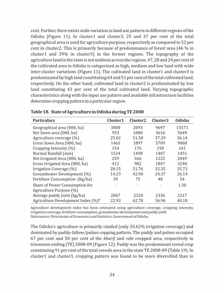
18. State of Agriculture in Odisha during TE 2008 34
19. Cluster & season wise area under different crops in Oidsha in TE-2008-09
38
1. Block-wise groundwater development (%) in Odisha 8
2. Classification of districts using K-means clustering analysis 12
3. Trend in groundwater development (%) in each cluster 15
4. Block-wise trend in water table in pre-monsoon season during 1997-2009 16
5. Block-wise trend in water table in post-monsoon season during 1997-2009 16
6. Block wise discharge rate (liter per second) in Odisha 17
7. Block–wise draw-down (meter) in Odisha 17
8. Composition of groundwater structures in different clusters in 2006-07 20
9. Changing share (%) of groundwater structures over the years 20
10. Electricity consumption for agriculture purpose and its share in total consumption over the years 27
11. Cluster-wise land use pattern in Odisha in 2008-09 36
12. Cluster and season wise cropping pattern (the share of crops in gross cropped area) in Odisha in TE 2008-09 37
13. The share (%) of Kharif paddy area in total high, medium & low land 38
1. INTRODUCTION
Groundwater plays a vital role in agricultural development by enhancing the
productivity of other inputs and by providing assured irrigation to the farmers.
Because of the land augmenting character and assured irrigation water, groundwater
development has always been the priority area by the policy makers. In agriculture
sector, importance of groundwater has been increasing manifold due to factors inter
alia technological breakthrough in extraction technology, soft loans for installation of
groundwater extraction mechanism and remunerative relative price ratio in favour of
water intensive, commercial and horticultural crops. Groundwater accounts for more
than 55 per cent of India's net irrigated area; however only 31 per cent of known
groundwater potential has been developed hitherto. Thus, at aggregate level, there is
ample opportunity to develop groundwater. However, there is a wide inter as well as
intra regional disparity as far as groundwater development is concerned. In some
parts of the country, such as Punjab, Western Uttar Pradesh, Gujarat, Tamil Nadu, etc.,
cases of groundwater over-exploitation have been noticed (GOI, 2001). On the other
hand, in the Eastern part of the country, level of groundwater development is very
low. The major concern at the national level nowadays is the sustainable agricultural
growth through equitable development of groundwater. This requires region specific
policy interventions in various aspects of groundwater development for irrigation
purposes.
As groundwater extraction primarily depends on mechanical devices, reliable,
economically accessible and efficient source of energy assumes a significant
importance. In the Odisha state of eastern India, utilization of groundwater and
energy use for the irrigation purpose is far less than other regions of similar hydro-
geological and climatic situations. Further, though Odisha was one of the first few
states to take initiatives in energizing the irrigation system, it lags behind in
implementation due to slow pace of electrification. Alternatively, diesel/kerosene
operated groundwater extraction pumps are becoming popular among the farmers.
Use of these alternative sources of energy for groundwater extraction depends on
various socio-economic (metered/flat rate tariff of electricity, subsidy, reliable
supply, etc) and political factors. Thus, a study on different aspects of groundwater
development and energy use pattern for irrigation in Odisha will provide a feedback
to the policy makers to formulate suitable energy policy for the holistic and
sustainable development of this precious natural resource. This, in turn, will emerge
as a precursor for the development of agriculture as a whole.
1
2. BACKGROUND
Literature related to groundwater development and energy use in irrigation in
Odisha as well as different parts of the country has been reviewed. The studies
revealed the increasing dominance of groundwater as a source of irrigation in the
nation. Of the addition to net irrigated area of about 29.75 million hectares between
1970 and 2007, groundwater accounted for 24.02 million hectares (80%). On an
average, between 2000-01 and 2006-07, about 61% of the irrigation in the country
was sourced from groundwater. The share of surface water has declined from 60% in
the 1950s to 30% in the first decade of the 21st century. The most dramatic change in
the groundwater scenario in India is that the share of tube wells in irrigated areas
rose from a mere 1% in 1960-61 to 40% in 2006-07. By now, tube wells have become
the largest single source of irrigation water in India (Shankar, et al. 2011). Though
only 58 per cent of the total groundwater has been developed in the country, there
existed wide spatial variation in its development. In many parts of the country such as
Punjab, Haryana, Rajasthan, Tamil Nadu, groundwater development is more than
sustainable level (CGWB, 2010). A more recent assessment by NASA showed that
during 2002 to 2008, three states (Punjab, Haryana and Rajasthan) together lost 3about 109 km of water due to decline in water table to the extent of 0.33 metres per
annum (Rodell et al 2009). On the other hand, in Eastern region, groundwater
development is less than 50 per cent. In Odisha, groundwater development is only 26
per cent (Govt. of Odisha, 2010) with wide variability across different districts due to
geological and socio-economic constraints. Lack of development of groundwater has
been thought to be the most important reason for stagnating agriculture in Eastern
India (Dhawan, 1982). The major foodgrains producing states of Haryana, Punjab and
Rajasthan in Northwest India are overexploited to the tune of 109-145%. On the
other hand, there is large scope for developing and utilizing groundwater for
irrigation in the poverty-ridden eastern states of Assam, Bihar, Chhattisgarh,
Jharkhand, Odisha and West Bengal since 58-82 % groundwater remains
underdeveloped and unutilized for irrigation. India's food security will be ensured
through the second green revolution in the high productivity potential eastern states
(Sharma, 2009). Groundwater irrigation has the potential of unleashing
unprecedented agrarian boom in Eastern India. However, due to a multitude of policy
differences coupled with varying agrarian structures, the beneficial impact of
groundwater has not been realized equally everywhere (Ballabh et al, 2002). Swain et
al. (2009) attempted to analyze the process of regional agricultural development in
the State of Odisha and identify the determinants of differential agricultural growth.
The results showed that four coastal districts (Balasore, Cuttack, Puri, and Ganjam)
and two districts of central table land area (Sambalpur and Bolangir) are
agriculturally more advanced than other districts in the three references years over
2
three decades (1980-81 to 1998-99). The agricultural success of four coastal districts
is due to well-developed irrigation facilities and vast tracts of plain and fertile land
comprising alluvial soil. The crux of the groundwater challenge in India is that there
is extreme overexploitation of the resource in some parts of the country coexisting
with relatively low levels of extraction in others (Shankar et. al., 2011). Along with the
development of groundwater irrigation, the contribution of groundwater irrigation
to the overall agricultural growth is estimated to have increased significantly in India.
Apart from directly benefiting the farmers having own groundwater structures, the
emergence of groundwater market has also benefited millions of non-well owning
farmers (Moorthy, 2008). Energy plays an important role in groundwater extraction
and various studies examined its relationship with groundwater development and
suggested that reliable electricity supply has a potential for efficient use of
groundwater. The studies have ascertained the impact of power tariff in the farm
sector on efficiency, equity and sustainability in groundwater use, and its overall
socio-economic viability thereof (Singh, 2008). Overall, the empirical evidences
reinforce the fact that the raising power tariff in the farm sector would be socio-
economically viable to achieve efficiency, equity and sustainability in groundwater
use. Sethi et al (2006) developed models to allocate available land and water
resources optimally on seasonal basis so as to maximize the net annual return in
Balasore district of Odisha, considering net irrigation water requirement of crops as
stochastic variable. The study reveals that 40% deviation of the existing cropping
pattern is the optimal that satisfies the minimum food requirement and maintain geo-
hydrological balance of the basin. The sensitivity analysis of conjunctive use of
surface water and groundwater shows that 20% surface water and 30% groundwater
availability as the optimum water allocation level. The proposed cropping and water
resources allocation policies of the developed models were found to be
socioeconomically acceptable that maintained the balance of the entire system,
considering all the constraints and restrictions imposed. The National Water Policy
calls for the conjunctive use of all the available water resources. These are rainwater,
river and surface water sources, groundwater, sea water and recycled waste water.
The conjunctive use of ground and surface water can help to improve cropping
intensity by using surface and rainwater during kharif and groundwater during rabi
and summer seasons. Integrated water resources management is vital for
maximizing the benefits of the available irrigation water.
3. DATA AND METHODOLOGY
The study is primarily based on secondary data on different hydro-geological, socio-
economic and energy use aspects collected from published sources of various
Government departments such as Central Groundwater Board (Bhubaneswar),
3
Directorate of Groundwater Survey & Investigation (Government of Odisha), Ministry
of Water Resources (Minor Irrigation Census), Directorate of Economics and
Statistics, etc. To provide a meaningful interpretation of the data, tabular, multivariate
and econometric analyses have been done. Tabular analysis has been done to examine
spatial and temporal groundwater development, sector-wise utilization, irrigation
potential created and utilized and constraints analysis. Further, log-linear regression
analysis has been done to establish relationship between groundwater development
and agricultural income in Odisha as follows;x
Log (Y) = c + b Log (X) + e … (1)where,
Y= per hectare net district domestic product from agriculture (Rs/ha)c = intercept to be estimated
b= regression coefficient to be estimatedX= groundwater development (%)e =unobserved error term
The regression coefficients were estimated using Ordinary Least Square (OLS)
technique. Thereafter, partial correlation coefficients (ρ) were estimated to identify
the factors affecting groundwater development and their inter-relationship.
… (2)
It is to be noted that correlation coefficient provide information about the nature of
the inter-relationship between two variables. To know the extent of influence of the
associated factors on the groundwater development, regression analysis using block
level data (210 out of 314 blocks for which uniform data was available) was also
attempted in which groundwater development was regressed with discharge, wells
(no.), draw-down and geology. To differentiate consolidated (hard-rock), semi
consolidated and non-consolidated (alluvial geology), dummy variable technique
was used. Blocks falling under alluvial areas were taken as a base category
(represented by intercept in the regression) and the groundwater development in
hard rock and semi-consolidated blocks was compared with alluvial blocks using the
estimated coefficients.
Groundwater development in Odisha exhibits wide inter-regional variations due to
varied hydro-geological conditions, agro-climatic features, infrastructure and other
socio-economic constraints. Therefore, an attempt was made to delineate regions of
similar hydro-geological properties and infrastructure development using k-means
cluster (multivariate) analysis. Groundwater development (%), discharge
(litre/second), draw-down (m), villages electrified (%) and seasonal water
fluctuation (meter) variables were considered for cluster analysis. Cluster analysis is
Correlation coeff.
4
an exploratory data analysis tool which aims at sorting different objects into groups in
a way that the degree of association between two objects is minimal if they belong to
the same group and maximal otherwise. Cluster analysis is used to discover
structures in data but without providing an explanation/interpretation why they
exist. K-means cluster analysis is an algorithm to classify or group objects based on
attributes/features into k number of group, k is positive integer number. The
grouping is done by minimizing the sum of squares of distances between data and the
corresponding cluster centroid. In k-means cluster analysis, first number of cluster K
is determined and cetroid or centre of these clusters is assumed. Any random objects
as the initial centroids or the first k objects can serve as the initial centroids. Then the
k-means algorithm will do the following three steps until convergence.
1. Determine the centroid coordinate
2. Determine the distance of each object to the centroids
3. Group the objects based on minimum distance (find the closest centroid)
Distance between each object and centroid is obtained by estimating Euclidean 2 ½
distance [distance(x,y) = {Σ (x - y ) } ] which the geometric distance in the i i i
multidimensional space. The procedure is repeated till the convergence criterion is
obtained. The convergence criterion represents a proportion of the minimum
distance between initial cluster centers, so it must be greater than 0 but not greater
than 1. If the criterion equals 0.02, for example, iteration ceases when a complete
iteration does not move any of the cluster centers by a distance of more than 2% of the
smallest distance between any initial cluster centers.
The districts of Odisha have been divided into three distinct clusters and comparative
analyses of different aspects of groundwater development and utilization have been
done across these clusters. An attempt was also made to quantify the variations in
aquifer properties and groundwater development within each cluster by estimating
coefficient of variation (CV) as follows;
The long-run sustainability of groundwater resources in the state was examined by
analyzing the trend (increasing/decreasing/no change) in water table (1997 to
2009) for each administrative block (314) in both pre-monsoon and post-monsoon
season by fitting the time-series regression functions. In the time–series analysis,
water table depth was regressed with the time variable after examining the
stationarity condition of the time series. The coefficients (intercept and slope) were
estimated using OLS (Ordinary Least Square) technique. The sign (+/-), significance
...(3)
5
level and value of slope variable in the function indicate the direction and rate of
change in the water table during the period under consideration.
The energy use aspects of groundwater irrigation were studied by examining the
trend in electricity consumption for agriculture purpose, distribution of groundwater
structures across alternative sources of energy and cost of groundwater extraction
using alternative energy sources (Diesel/Electricity) in different clusters. The steps
involved in estimation of cost of per cubic meter groundwater extraction are as
follows;
1. Estimation of average horse power (hp) of the pumps used in groundwater
structures (Shallow Tubewells/Deep Tubewells/Dugwells) across different
clusters. Average horse power (hp) was estimated by weighted average using the th
recent (4 ) Minor Irrigation (MI) census data. Thereafter, average hp was
expressed in terms of Energy (Kilowatt) by multiplying with the factor 0.746. For
man/animal operated dugwells, 0.28 KW {(average of 0.06 (male), 0.048
(female) and 0.746 (drought animal)} energy was used (Srivastava, N.S.L., 2002).
2. Estimation of “total head” using following formula;
Total Head (m) = Water table (m) + draw down(m) + friction loss ... (4)
10 per cent of the water table and draw down was taken as friction loss. Average
water table and draw down for each cluster was estimated using the data
collected from Central Groundwater Board and Directorate of Survey &
Investigation (Government of Odisha).
3. Estimation of average groundwater draft (l./sec.) using following formula;
... (5)
Pump efficiency was assumed as 40%. Thereafter, groundwater extraction in the
full year was estimated using the information such as number of pumping days
in monsoon and non-monsoon seasons and average pumping hours/day. The
number of pumping days in monsoon and non-monsoon season were taken as
50 and 120, respectively (Directorate of Groundwater survey & Investigation,
Govt. of Odisha). Average pumping hours/day for different groundwater th
structures were calculated by weighted average using recent (4 ) Minor
Irrigation (MI) census data.
4. Estimation of energy consumed to lift one cubic meter of groundwater
(KWhr/cum). For diesel operated pumps, it was found from the farmers'
6
response that 1 hp pump consumes about 0.25 liter diesel in one hour.
Thereafter, energy was expressed in monetary terms (Rs/cum.) by multiplying
with Rs.45 per liter for diesel and Rs 1.10 per Unit (KW) for electricity.
5. Estimation of total annual amortized cost of groundwater structure (Shallow
Tubewell/Deep Tubewells/Dugwell) as sum of total amortized digging cost,
total amortized pump cost and maintenance cost.
...(6)
where,
A = amortized cost of digging/pump (Rs.)
CB= initial Cost digging/pump (Rs.)
i = interest rate (6%)
n = life of groundwater structure
For cluster 1 and cluster 3 (Hard rock areas), average life of groundwater
structure was taken as 15 years, while for cluster 2 (Alluvial/coastal) average life
of groundwater structure was taken as 20 years. Average life of pump was taken
as 10 years. Annual maintenance cost was taken as 5 % and 1% of pump cost for
diesel and electric operated pumps, respectively.
6. Estimation of total cost of per cubic meter groundwater extraction (Rs/cum) as
sum of total annual amortized cost (Rs/cum) and energy cost (Rs/cum).
Thereafter, the share of alternative sources of energy (diesel/electricity) in total
groundwater extraction cost was examined across different clusters and
groundwater structures and implication of government subsidy on these energy
sources was diagnosed.
As agriculture is the major consumer of groundwater resources, its performance was
examined in different clusters by estimating agriculture development index (ADI) as
following;
... (7)
Where, ADI is agriculture development index which is average (with equal weight to th thall the indicators) of i indicator for j district. Agriculture coverage (share of
agricultural area in total geographical area), irrigation coverage (share of gross
irrigated area in gross cropped area), cropping intensity (net sown area/gross sown
( )
( )´ + ´
=+ -
n
n
CB 1 i iA
1 i 1
7
area), paddy yield, groundwater development and fertilizer consumption (kg/ha)
were taken as the individual indicators to estimate composite agriculture
development index in each cluster. Index for individual indicator was calculated as
follows;
... (8)
th thwhere Y is the i indicator for j district. Inter-cluster variations in agricultural ij
performance were examined and inferences were drawn.
4. RESULTS AND DISCUSSION
4.1. Different Aspects of Groundwater Development in Odisha
4.1.1. Status of Groundwater Resources in Odisha
Gross groundwater recharge has been estimated as 17.77 billion cubic meter (BCM)
in Odisha through different sources (Table 1). Rainfall contributes 71 per cent in gross
groundwater recharge. With 1.09 BCM of natural groundwater losses, net
groundwater availability in Odisha is 16.69 BCM. Out of this, only 4.36 BCM
groundwater is drafted with irrigation sector extracting the highest (79.6 per cent).
Thus, overall groundwater development in Odisha stands only 26.14 per cent.
However, there exists wide variability in its development across different districts
ranging from 8.76 per cent in Malkangiri to 55 per cent in Bhadrak due to varying
hydro-geological and socio-economic conditions. Among the 314 blocks,
groundwater development in 23 coastal blocks is more than 50 per cent. At the same
time, in 25 hard rock blocks, groundwater development in less than 10 per cent.
Further, 36 and 6 coastal blocks are partially and fully affected by salinity problem,
respectively. Block-wise categorization into four quartile classes revealed that in 75
p e r c e n t o f t h e to t a l b l o c ks ,
groundwater development is less than
34 per cent and most of the blocks,
where groundwater development is
better, fall in coastal belt of the state
(Figure 1). For future, after reserving
groundwater for industry and
domestic uses for the next 25 years,
1.19 BCM and 0.84 BCM groundwater
is available for creation of additional
irrigation potential at 100 per cent and
70 per cent level of groundwater
development, respectively. Figure 1: Block-wise groundwater development (%) in Odisha
Legend
Odisha Blocks_Groundwater %
0 to 15
15 to 22
22 to 34
34 to 70
data not available
8
Table 1. Status of groundwater resources in Odisha in 2009-10
Figures within parentheses includes share in total groundwater draftSource: Directorate of Groundwater Survey and Investigation, Government of Odisha, 2011
4.1.2. Groundwater irrigation-agricultural income linkage in Odisha
Although groundwater constitutes a small share (6.14 %) in gross irrigated area
(GIA) in Odisha, it bears a positive relationship with the agricultural income. 2Estimated log-linear regression function revealed that about a quarter (R ) of the
agricultural income (Rs/ha) is dependent on groundwater (Table 2). The elasticity of
agricultural productivity with respect to groundwater development (estimated
coefficient) was positive (0.598) and significant at 1% level of significance, indicating
improvement in groundwater development will increase the agricultural income in
the state. It has been estimated that 47.75 per cent of the total ultimate irrigation
potential (8.8 Mha) in Odisha can be developed using groundwater and till now only
13 per cent (5.5 lakh ha) of the Ultimate Irrigation Potential (UIP) has been created
using groundwater resources. Thus, there is enough scope for improving agricultural
income in the state through sustainable groundwater development.
Table 2. Results of regression analysis between agricultural income and groundwater development in Odisha
Particular EstimatesConstant 8.569*
(0.631)
Groundwater development (log) 0.598*(0.199)
R2
0.244
No. of observations
30
Dependent variable: Per hectare net district domestic product from agriculture (Rs/ha) in logarithmic form*significant at 1% degree of significanceFigures within parentheses are standard errors of estimated coefficients
9
4.1.3. Factors affecting groundwater development in Odisha
The development of groundwater resources in a location is outcome of a complex set of inter-related hydro-geological, socio-economic, agriculture and infrastructure related factors. To identify major factors affecting groundwater development in Odisha, partial correlation coefficient was estimated using district level data. The variables such as discharge and draw-down were taken as proxy for hydro-geological conditions, while electrified villages (%), per capita income (net district domestic product) and fertilizer consumption (kg/ha) were taken as proxy for infrastructure development, economic conditions of the farmers and level of input use in agriculture, respectively. The estimated correlation coefficient between groundwater development and other variables was significant and positive except for draw-down (Table 3).
Table 3. The estimated correlation coefficient between groundwater development and other factors
*. Correlation is significant at the 0.05 level (2-tailed).**. Correlation is significant at the 0.01 level (2-tailed).
The correlation coefficient between discharge and groundwater development was 0.81 which indicated that the areas with high discharge (lit/sec) are conducive for groundwater development. On the other hand, high draw-down affects the groundwater extraction negatively as shown by negative correlation coefficient between groundwater development and draw down (-0.53). The installation of groundwater structure primarily involves private investment. Therefore, income of the farmers was found to be an important determinant (positive correlation coefficient) of the groundwater development in Odisha. Similarly, availability of electricity was found to be positively affecting groundwater development as shown by high and positive correlation coefficient. Moreover, positive correlation coefficient between groundwater development and fertilizer consumption indicated that irrigation and fertilizer consumption are complement to each other. The assured availability of irrigation induces farmers to apply more fertilizer to maximize farm profit. It is to be noted that per hectare fertilizer consumption in the state (54 kg/ha) was less than half of the national average (118 kg/ha) in TE 2008-09. Thus, assured irrigation through groundwater development has the potential to improve fertilizer consumption and therefore agricultural productivity in Odisha.
10
The correlation coefficient indicates nature of relationship between two variables. To know the extent of influence of these variables, regression analysis was done using block level data (Table 4). It is to be noted that per capita income, electrified villages and fertilizer consumption could not be taken as explanatory variables in regression analysis due to unavailability of consistent data.
Table 4. Estimated parameters of regression analysis
Variables Estimated ParameterConstant 41.191*
(4.195) Discharge 0.209*
(0.071)
Consolidated (Hardrock) geology
-18.956* (2.978)
Semi-consolidated geology
-11.311* (4.054)
Wells
7.261E-03* (0.001)
Draw down
-9.149E-02
(0.087)
No. of observations
210
R2 0.58
Dependent variable: groundwater development*significant at 1% level of significanceFigures within parentheses are standard error of the estimated parameters
From the estimated parameters, it was found that groundwater development in
consolidated and semi-consolidated areas are significantly lower by 18 and 11 per
cent than alluvial region of the state. The groundwater development in alluvial areas
is represented through the intercept value of the regression. The positive coefficient
of discharge and negative coefficient of draw-down indicated that groundwater
recharge activities in the areas of low discharge and high draw-down would improve
the groundwater development.
4.1.4. Classification of districts using K-means clustering technique
Odisha exhibits wide inter-regional variability in hydro-geological properties and
socio-economic conditions leading to differential groundwater development across
different regions. Therefore, multivariate (K-means clustering technique) analysis
was used to classify districts, exhibiting similarity in attributes (groundwater
development, discharge, drawdown, electrified villages and water level fluctuation),
into 3 distinct clusters (Figure 2).
11
Figure 2. Classification of districts using K-means clustering analysis
The aquifer properties, infrastructure development (villages electrified taken as proxy) and number of districts in each cluster are given in table 5. Mean values of the attributes in each cluster was found to be significantly different from each other except water level fluctuation as shown by the analysis of variance (Table 6). Groundwater development was found to be highest (42.90 %) in cluster2 and least (14.23 %) in cluster 1. It is to be noted that cluster2 exhibited more favourable aquifer properties (highest discharge rate, least drawdown and least water level fluctuation) and infrastructure development (highest electrified villages) as compared to other clusters. On the other hand, mean values of aquifer properties and infrastructure development in cluster1 was unfavourable leading to least (14.23%) groundwater development in the districts included in this cluster. Further, all the 7 districts of cluster 2 are located in coastal/alluvial region (with favourable aquifer properties) of the state, while all the 6 districts of cluster 1 are located in hard rock (with u n favo u ra b l e a q u i fe r p ro p e r t i e s ) re g i o n o f t h e s t a te . H oweve r, favorable/unfavourable aquifer properties were found to be complemented by the better/least infrastructure development (electrified villages) for groundwater development in the respective regions. Thus, improvement in infrastructure related to groundwater can play a crucial role in its development especially in less developed regions of the state. Groundwater development in cluster3 containing 17 districts was 24.37 per cent.
Legend
Cluster 1
Cluster 2
Cluster 3
SUNDERGARH
NUAPADA BOLANGIR BOUDH
BARGARH SAMBALPUR
DEOGARH
JHARSUGUDA
MAYURBHANJ
KEONJHAR
BALASORE
BHADRAK
JAJPUR
KENDRAPADACUTTACK
JAGATSINGHPUR
PURI
KHURDA
DHENKANAL
ANGUL
NAYAGARH
GANJAM
PHULBANI
GAJAPATI
RAYAGADA
KORAPUT
MALKANAGIRI
NAWARANGPUR
SONEPUR
KALAHANDI
12
Table 5. Cluster-wise aquifer properties and infrastructure development (mean values)
Variables Cluster 1 Cluster 2 Cluster 3
Groundwater development (%) 14.23 42.90 24.37
Discharge (litre/second) 3.07 35.37 5.21
Drawdown (meter)
21.89
10.44 20.27
Villages electrified (%)
11.88
88.32 69.15
seasonal water level fluctuation (meter)
2.72
2.20 2.315
No. of districts 6 7 17
Districts categorized under cluster1 and cluster3 have hard rock geology, while
districts in cluster2 fall in alluvial/coastal belt of Odisha. The favourable aquifer
properties (high discharge, low draw-down and high water level) in coastal areas
(cluster2) also results in comparatively low energy requirement to lift the
groundwater. However, these areas are hydrologically sensitive to sea-water
intrusion and 42 coastal blocks are already partially or fully affected by the salinity
problem. Hence, safe pumping options should be followed in order to use the
groundwater on sustainable basis in coastal areas. On the other hand, in hard rock
region (cluster1 and cluster3), Poor groundwater development is primarily due to
low discharge, high draw-down and heterogeneity in aquifer properties within the
small areas. The unfavorable hydro-geological conditions also results in higher
energy requirement to extract groundwater in these areas. Thus, the associated
problems and therefore strategies for the sustainable groundwater development in
different hydro-geological settings (hard rock/coastal) would be different.
Table 6. Analysis of variance (ANOVA) in cluster analysis
Variables Cluster Error F Sig.Mean
Square
df Mean
Square
df
Groundwater Development
1430.76 2
52.35
27
27.33 0.00
Discharge
2542.67
2
19.08
27
133.26 0.00
Draw down
288.02
2
16.23
27
17.74 0.00
Villages electrified
10394.53
2
144.32
27
72.02 0.00
Water level fluctuation 0.49 2 .25 27 1.95 0.16
Note: The F tests should be used only for descriptive purposes because the clusters have been chosen to maximize the differences among cases in different clusters. The observed significance levels are not corrected for this and thus cannot be interpreted as tests of the hypothesis that the cluster means are equal.
13
4.1.5. Inter-cluster and intra-cluster variations in groundwater development
Out of the 16.69 BCM of net groundwater reserve, cluster3 endows 9.47 BCM
groundwater reserve as it contains largest number (186) of administrative blocks of
the state (Table 7). Similarly, cluster3 dominates in total groundwater draft. Further,
there exists wide variability in groundwater resources and its utilization in the state
as well as different cluster. Estimated coefficient of variation (CV) for net
groundwater resources for the state was 45 per cent ranging from 38 per cent in
cluster3 to 57 per cent in cluster2. The estimated CV for total groundwater draft for
the state was 80 per cent ranging from 51 per cent in cluster3 to 67 per cent in
cluster2. High CV in cluster2 was primarily due to presence of saline affected area in
which groundwater draft is very less. Among different sectors, irrigation was the
dominant user of groundwater in all the clusters. However, the use of groundwater for
domestic purpose was more pronounced in cluster1 and cluster3 as compared to
cluster2. In cluster2, about 87 per cent of the total groundwater draft is used for
irrigation purpose.
Table 7. Groundwater resources, draft and its development within each cluster
Particulars Cluster1 Cluster2 Cluster3 OdishaNet Ground water resources (BCM) 3.17
(44)
4.06 (57)
9.47 (38)
16.69(45)
Groundwater Draft (BCM)
0.40 (59)
1.68 (67)
2.28 (51)
4.36(80)
Irrigation (% of total draft)
67.83
86.81
76.50
79.6
Domestic (% of total draft)
26.01
10.76
20.00
16.99
Industrial (% of total draft)
6.15
2.43
3.50
3.41Groundwater development (%)
14.23
(42)
42.90
(39)
24.37
(43)
26.14(54)
No. of blocks 57 71 186 314
Figures within parentheses are coefficient of variation (CV) estimated using block level data
The development of groundwater exhibits wide inter-cluster as well as intra-cluster
variations. The groundwater development ranges from 14.23 per cent in cluster1 to
42.90 per cent in cluster2 with the overall development of 26.14 per cent in the state.
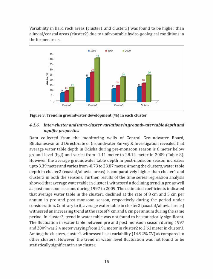
Temporally, groundwater development in Odisha has increased from 15 per cent in
1999 to 26 per cent in 2009 (Figure 3). The increasing trend in groundwater
development was found in all the clusters. Groundwater development has increased
from 9 per cent to 14 per cent in cluster1, from 23 to 43 per cent in cluster2 and 13 to
24 per cent in cluster3 during 1999 to 2009. However, the rate of increase in
groundwater development was highest in cluster3 (90%) followed by cluster2 (83%)
and cluster1 (59%). Further, high value of estimated coefficient variation using block
level data for the state (54%) indicated wide variability in groundwater development.
14
Variability in hard rock areas (cluster1 and cluster3) was found to be higher than
alluvial/coastal areas (cluster2) due to unfavourable hydro-geological conditions in
the former areas.
4.1.6. Inter-cluster and intra-cluster variations in groundwater table depth and
aquifer properties
Data collected from the monitoring wells of Central Groundwater Board,
Bhubaneswar and Directorate of Groundwater Survey & Investigation revealed that
average water table depth in Odisha during pre-monsoon season is 6 meter below
ground level (bgl) and varies from -1.11 meter to 28.14 meter in 2009 (Table 8).
However, the average groundwater table depth in post-monsoon season increases
upto 3.39 meter and varies from -0.73 to 23.87 meter. Among the clusters, water table
depth in cluster2 (coastal/alluvial areas) is comparatively higher than cluster1 and
cluster3 in both the seasons. Further, results of the time series regression analysis
showed that average water table in cluster1 witnessed a declining trend in pre as well
as post monsoon seasons during 1997 to 2009. The estimated coefficients indicated
that average water table in the cluster1 declined at the rate of 8 cm and 5 cm per
annum in pre and post monsoon season, respectively during the period under
consideration. Contrary to it, average water table in cluster2 (coastal/alluvial areas)
witnessed an increasing trend at the rate of 9 cm and 6 cm per annum during the same
period. In cluster3, trend in water table was not found to be statistically significant.
The fluctuation in water table between pre and post monsoon season during 1997
and 2009 was 2.4 meter varying from 1.91 meter in cluster2 to 2.61 meter in cluster3.
Among the clusters, cluster2 witnessed least variability (14.92% CV) as compared to
other clusters. However, the trend in water level fluctuation was not found to be
statistically significant in any cluster.
Figure 3. Trend in groundwater development (%) in each cluster
-
5
10
15
20
25
30
35
40
45
Cluster1 Cluster2 Cluster3 Odisha
9
23
13 15
11
29
16 18
14
43
24 26
GW
de
v.(%
)
1999 2004 2009
15
Table 8. Cluster-wise trend in water table and aquifer properties in Odisha
Particulars Cluster1 Cluster2 Cluster3 OdishaWater level (meter) in 2009#
Pre-monsoon
6.13
(-1.11 to 28.14)
5.03 (-0.50 to 15.25)
6.39 (-0.95 to 18.92)
6.02(-1.11 to 28.14)
Post-monsoon
3.63
(0.02 to 23.87)
2.73
(-0.45 to 11.15)
3.57
(-0.73 to 15.55)
3.39(-0.73 to 23.87)
Trend (decline/increase/no) during 1997-2009$
Pre-monsoon
-0.089**
(0.034)
0.095***
(0.020)
0.007
(0.020)
0.009(0.018)
Post monsoon
-0.057*
(0.033)
0.068***
(0.019)
0.009
(0.026)
0.009(0.023)
Water level fluctuation between 1997-2009$
Mean
2.36
1.91
2.61
2.40
Standard deviation
0.60
0.29
0.45
0.40
Coefficient of Variation (%)
25.62
14.92
17.22
16.71Trend
0.032
(0.046)
0.057
(0.033)
-0.027
(0.021)
0.001(0.031)
Discharge
(lit/sec)
Mean
3.07
35.37
5.21
11.88
Standard deviation
3.61
20.19
6.36
17.58Coefficient of Variation (%)
118
57
122
148Draw-down (meter)
Mean 21.89 10.44 20.27 18.84Standard deviation 9.06 6.03 8.57 9.15
Coefficient of Variation (%) 41 58 42 49
#Figures within parentheses are minimum and maximum value of water table$ figures within parentheses are standard error of the estimated regression parameter (time) *** significant at 1% level of significance, ** significant at 5% level of significance, * significant at 10% level of significance
Figure 4. Block-wise trend in water table in pre-monsoon season during 1997-2009
Figure 5. Block-wise trend in water table in post-monsoon season during 1997-2009
16
It is to be noted that average water table depth at cluster level give macro level
scenario. Therefore, trend in water table was further examined at disaggregated
(block level) in both pre and post monsoon period and results are presented in figure
4 and 5. The results of time series regression analysis showed that in 140 blocks (45%
of the total administrative blocks), there was no significant change in water level in
pre-monsoon season during 1997 to 2009. In 92 blocks (30% of the blocks), water
table was found to be increased. This indicated the scope for accelerating
groundwater utilization in the blocks with no change/increase (232 blocks) in water
table during the period under consideration. On the other hand, in 77 blocks (25% of
total blocks), water table witnessed declining trend in pre-monsoon season during
1997-2009. This necessitates implementation of groundwater recharge activities in
these 77 blocks to ensure sustainable development of groundwater in the state. The
name of the blocks falling in each category (increasing trend/decreasing trend/no
change) is given in Appendix.
The diagnosis of aquifer properties (discharge and draw-down) revealed that
discharge (ℓ./sec) varies from 3 ./sec in cluster1 to about 35 ./sec in cluster2 with
the average discharge of 11.88 ./sec in the state. Low aquifer discharge in cluster1
necessitates adoption and popularization of micro-irrigation technology which suits
well in low discharge rate scenario. Further, cluster1 and cluster3 exhibited very high
variability (CV value of >100) in discharge rate as compared to cluster2 which has
definite implications on groundwater development in the state. Draw-down was
found to vary from 10.44 meter in cluster2 to 21.89 meter in cluster1 with the average
draw-down of 18.84 meter in the state. High value draw-down in cluster1 and
cluster3 are primarily due to low recuperation rate of geological formations in these
areas. On the other hand, in alluvial areas (cluster2), comparatively low value of draw-
ℓ ℓ
ℓ
Figure 6. Block wise discharge rate (liter per second) in Odisha
Figure 7. Block–wise draw-down (meter) in Odisha
17
down is due to high recharge rate. However, care should be taken while interpreting
the value of draw-down as its value will depend largely on the type of groundwater
structure (shallow tubewell/deep tubewell/dugwell) used for its extraction and
hours of pumping.
4.1.7. Temporal and spatial variations in groundwater structures and
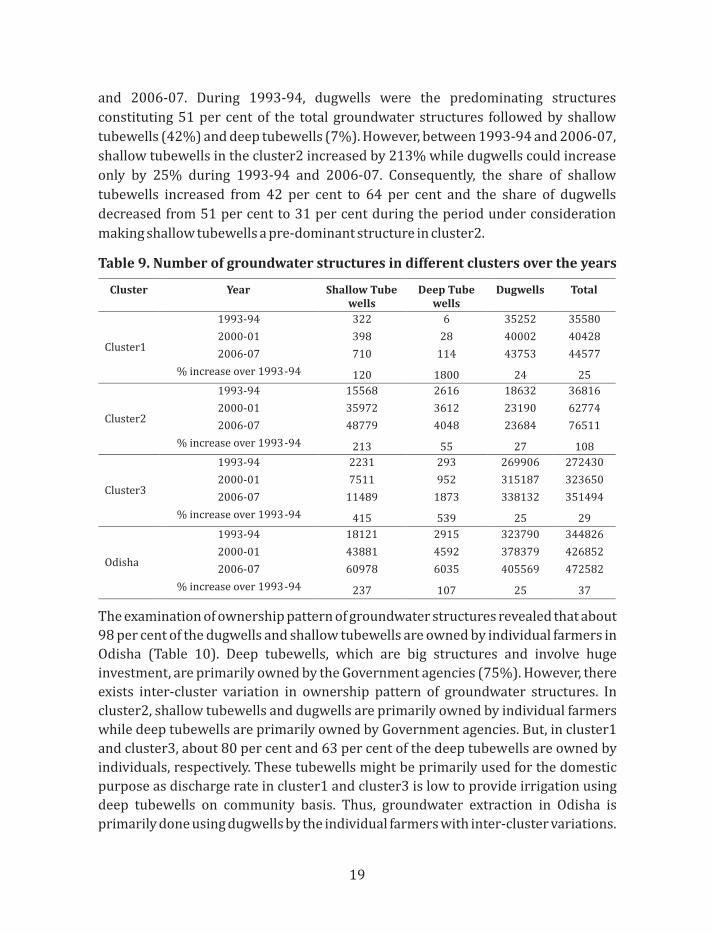
ownership pattern
The number and type of the groundwater structure bears a significant impact on
groundwater extraction and thus its development. The trend in number and
composition (shallow tubewells/deep tubewells/dugwells) of groundwater
structures has been studied across different clusters in Odisha using district level nd rd thdata of 2 (1993-94), 3 (2000-01) and 4 (2006-07) minor irrigation census.
Presently, there are about 4.7 lakh groundwater structures in the state (Table 9).
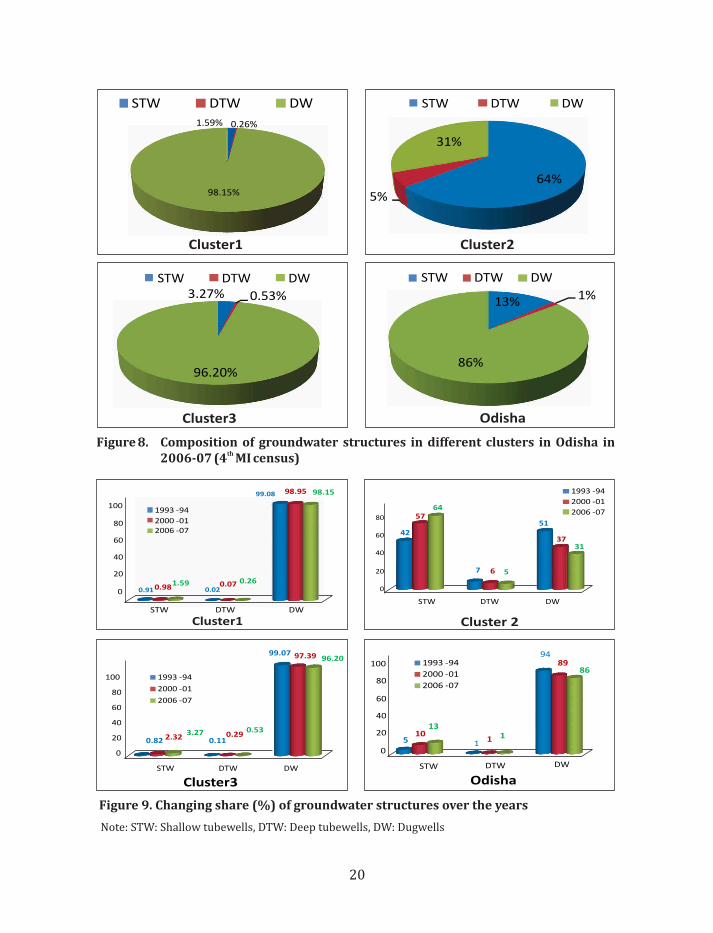
However, examination of the composition of groundwater structures revealed that
dugwells are the predominant structure constituting 86 per cent (about 4 lakh) of the
total groundwater structures in the state (Figure 8). The shallow tubewells and deep
tubewells constituted 13 per cent and 1 per cent of the total groundwater structures
in 2006-07, respectively. Temporally, the groundwater structures have increased by
37 per cent between 1993-94 and 2006-07. However, the rate of increase was not
uniform across different type of groundwater structures and clusters (Figure 9).
Among the groundwater structures, shallow tubewells witnessed maximum increase
of 237 per cent followed by deep tubewells (107%) and dugwells (25%).
Consequently, the share of dugwells in total groundwater structure declined from 94
per cent in 1993-94 to 86 per cent in 2006-07 (Figure 9). On the other hand, the share
of shallow tubewells has increased from 5 per cent to 13 per cent during the period
under consideration. Among the clusters, the rate of increase in groundwater
structures was highest (102%) in cluster2 followed by cluster3 (29%) and cluster1
(25%).
Composition of groundwater structures was not found to be uniform across different
clusters due to varying hydro-geological conditions and other socio-economic
constraints. In cluster1 and cluster3, dugwell was the predominant structure
constituting 98 per cent and 91 per cent of the total groundwater structures in 2006-
07. Cluster1 and cluster3 falls in hard rock areas and dugwells are the most feasible
structures in these areas. As hard rock occupies largest geographical area (>80%) of
the state, this may be an important reason for the dominance of dugwells. On the
other hand, in cluster2, shallow tubewells were the predominant structures
constituting 64 per cent of total groundwater structures followed by dugwells (31%)
and deep tubewells (5%) in 2006-07. Temporally, a structural shift in the
composition of groundwater structures was observed in cluster2 between 1993-04
18
and 2006-07. During 1993-94, dugwells were the predominating structures
constituting 51 per cent of the total groundwater structures followed by shallow
tubewells (42%) and deep tubewells (7%). However, between 1993-94 and 2006-07,
shallow tubewells in the cluster2 increased by 213% while dugwells could increase
only by 25% during 1993-94 and 2006-07. Consequently, the share of shallow
tubewells increased from 42 per cent to 64 per cent and the share of dugwells
decreased from 51 per cent to 31 per cent during the period under consideration
making shallow tubewells a pre-dominant structure in cluster2.
Table 9. Number of groundwater structures in different clusters over the years
Cluster Year Shallow Tube wells
Deep Tube wells
Dugwells Total
Cluster1
1993-94
322
6
35252 35580
2000-01
398 28
40002 40428
2006-07
710
114
43753 44577
% increase over 1993-94
120
1800
24 25
Cluster2
1993-94
15568
2616
18632 36816
2000-01
35972
3612
23190 62774
2006-07
48779
4048
23684 76511
% increase over 1993-94
213
55
27 108
Cluster3
1993-94
2231
293
269906 272430
2000-01
7511
952
315187 323650
2006-07
11489
1873
338132 351494
% increase over 1993-94
415
539
25 29
Odisha
1993-94
18121
2915
323790 344826
2000-01 43881 4592 378379 426852
2006-07 60978 6035 405569 472582
% increase over 1993-94 237 107 25 37
The examination of ownership pattern of groundwater structures revealed that about
98 per cent of the dugwells and shallow tubewells are owned by individual farmers in
Odisha (Table 10). Deep tubewells, which are big structures and involve huge
investment, are primarily owned by the Government agencies (75%). However, there
exists inter-cluster variation in ownership pattern of groundwater structures. In
cluster2, shallow tubewells and dugwells are primarily owned by individual farmers
while deep tubewells are primarily owned by Government agencies. But, in cluster1
and cluster3, about 80 per cent and 63 per cent of the deep tubewells are owned by
individuals, respectively. These tubewells might be primarily used for the domestic
purpose as discharge rate in cluster1 and cluster3 is low to provide irrigation using
deep tubewells on community basis. Thus, groundwater extraction in Odisha is
primarily done using dugwells by the individual farmers with inter-cluster variations.
19
Figure 8. Composition of groundwater structures in different clusters in Odisha in th2006-07 (4 MI census)
1.59% 0.26%
98.15%
Cluster1
STW DTW DW
64%
5%
31%
Cluster2
STW DTW DW
3.27% 0.53%
96.20%
Cluster3
STW DTW DW
13% 1%
86%
Odisha
STW DTW DW
0
20
40
60
80
100
STW DTW DW
0.91 0.02
99.08
0.98 0.07
98.95
1.59 0.26
98.15
Cluster1
1993 -94
2000 -012006 -07
0
20
40
60
80
STW DTW DW
42
7
5157
6
37
64
5
31
Cluster 2
1993 -94
2000 -01
2006 -07
0
20
40
60
80
100
STW DTW DW
0.82 0.11
99.07
2.32 0.29
97.39
3.27 0.53
96.20
Cluster3
1993 -94
2000 -01
2006 -07
0
20
40
60
80
100
STW DTW DW
5 1
94
101
89
131
86
Odisha
1993 -94
2000 -01
2006 -07
Figure 9. Changing share (%) of groundwater structures over the years
Note: STW: Shallow tubewells, DTW: Deep tubewells, DW: Dugwells
20
Table10. Ownership pattern of groundwater structures in Odisha in 2006-07 (% of total)
STW: shallow tubewells, DTW: Deep tubewells, DW: Dugwells
4.1.8. Inter-cluster variations in groundwater irrigation potential
created (IPC) and its utilization (IPU)
Odisha's agricultural economy is primarily rainfed with only 35 per cent (31.77 lakh
ha) of the gross cropped area irrigated through different sources (Govt. of Odisha,
2010). Groundwater resources constitute only 6.14 per cent (1.97 lakh ha) of gross thirrigated area (4 MI Census). Although the irrigation potential created through
groundwater in the state is 5.5 lakh ha (Table 11), its utilization (IPU) is only 35.22 per
cent (1.97 lakh ha) in 2006-07 raising several efficiency issues in its utilization. The rd
pace at which IPC through groundwater increased between 2000-01 (3 MI census) th
and 2006-07 (4 MI census), due to massive Government support and incentives,
could not continue for IPU resulting into decline in the per cent utilization from 51.53
per cent to 35.68 per cent during the same period. Among different sources of
groundwater irrigation, dugwells predominated contributing 39.24 per cent and
43.08 per cent of the total IPC and total IPU, respectively in 2006-07. However, in
utilization of created potential, shallow tubewells outpaced dugwells with the per
cent utilization of 45.62. The per cent utilization of created potential declined for all
the sources with deep tubewells witnessing highest decline in 2000-2006. Poor
utilization of the irrigation potential through groundwater might be due to several
factors such as unfavourable hydro-geological conditions, frequent failure of wells,
poor maintenance, lack of assured electricity supply, saline water intrusion, etc.
21
Table 11. Irrigation potential created (PC) and irrigation potential utilized (IPU)
*figures within parentheses are share of IPC created through respective GW structure in total IPC
# figures within parentheses are the per cent utilization of created irrigation potential
STW: Shallow tubewell, DTW: Deep tubewells, DW: Dugwells
Cluster-wise diagnosis of IPC revealed the creation of irrigation potential is largely
affected by the type of groundwater structures. With only 13 per cent of the total
geographical area, 19 per cent of agricultural land, 24 per cent of groundwater
resources and 16 per cent of groundwater structures of the state, cluster2 constituted
about 52 per cent (2.88 thousand ha) of the total IPC of Odisha in 2006-07. This is
primarily because of dominance of shallow and deep tubewells in this region which
has larger irrigation command area as compared to dugwells. Shallow and deep
tubewells created 54 per cent (155 thousand ha) and 40 per cent (114 thousand ha)
of the total irrigation potential created in cluster2, respectively. Cluster1 and cluster3
constituted about 4 per cent and 44 per cent of the total IPC of Odisha in 2006-07,
respectively. In these clusters, dugwells were the predominating structures which
constituted about 75 per cent of the total IPC in the respective cluster. Although cluster2 constituted highest share in total IPC of the state, it exhibited least
(30.44%) utilization of already created potential as compared to other clusters in
2006-07 (Table11). The poor utilization of already created potential in cluster2 was
primarily because of deep tubewells which could utilize only 11 per cent of the IPC
created through it. Similarly, utilization of IPC through dugwells was only 29 per cent
in 2006-07 in cluster2. In cluster1 and cluster3, utilization of IPC was 45 per cent and
41 per cent in 2006-07, respectively with the declining trend over the years. The poor
utilization of the already created irrigation potential leads to loss of financial
22
resources in one hand and loss of opportunity to improve agricultural productivity
and income through advantages of assured irrigation on the other. Thus, the
groundwater sector in Odisha is suffering from the dual problem of under-
development of groundwater resources as well as under-utilization of the already
created irrigation potential. Thus, identification of factors responsible of poor
utilization of already created irrigation potential will go a long way to improve the
irrigation infrastructure in the state.
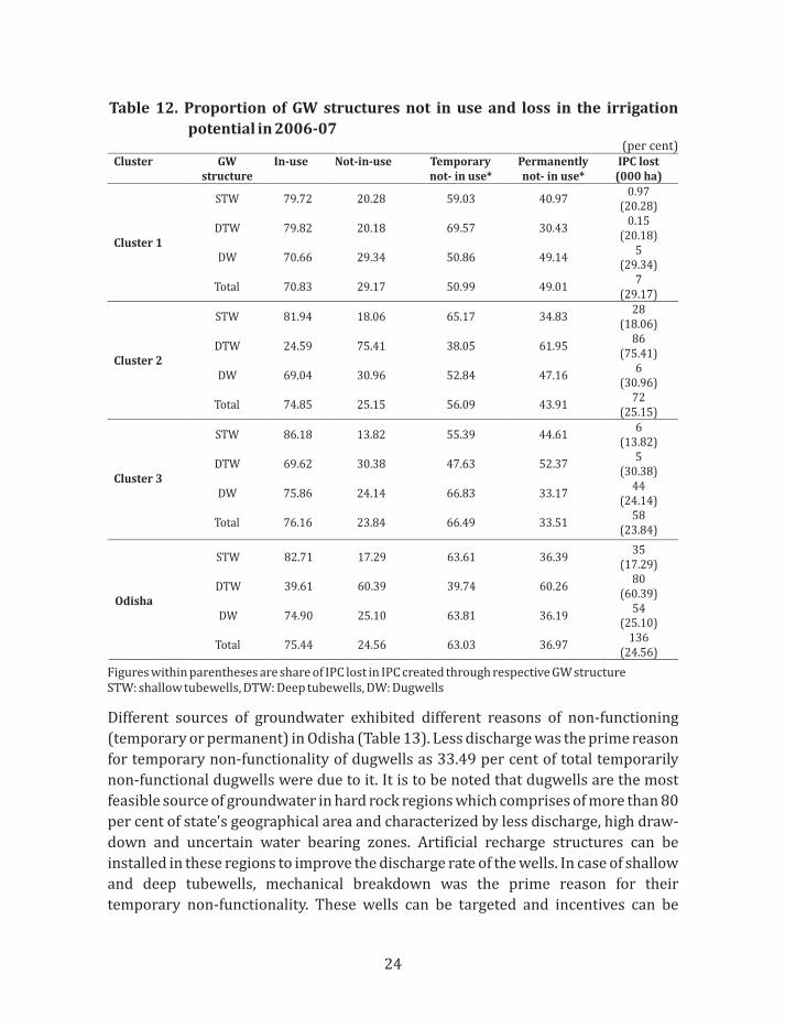
4.1.9. Constraints in groundwater irrigation in Odisha
Under-development and inefficient utilization of groundwater resources in Odisha
might be because of several hydro-geological, agro-climatic and socio-economic
constraints. However, non-functioning of the wells was found to be an important
reason of poor utilization of created irrigation potential. A perusal of table 12 reveals
that about a quarter of total groundwater structures in Odisha are not-in-use due to
temporary or permanent reasons. 63 per cent structures are not-in-use temporarily
and 37 per cent permanently. Non-functioning of groundwater structure resulted
into loss of 136 thousand hectare (24.56 per cent of IPC) irrigation potential annually
in Odisha. About 60 per cent (80.09 thousand ha) loss in the IPC is due to non-
functioning of deep tubewells alone which irrigate highest command area as
compared to other sources. Dugwells and shallow tubewells contributed 25 per cent
and 17 per cent loss in IPC in 2006-07.
Among the clusters, loss in the irrigation potential due to non-functioning of wells
was highest (72 thousand ha) in cluster2. This was primarily because of mass scale
non-functioning of deep-tubewells as about 75 per cent of the total deep-tubewells in
cluster2 were found to be defunct. As majority of these structures are owned and
maintained by Government agencies, mass scale non-functioning raises several
inefficiency issues in operation and maintenance of deep tubewells. Further, as deep
tubewells cover largest command area as compared to other wells, theses non-
functional wells can be targeted and revived which would involve much less
expenditure than to create new irrigation potential. Mass scale non-functionality of
this Government owned tubewells also sets a strong platform for transferring their
ownership to the farmers. Operation and management transfer to pani-panchayat/
water users' association (WUA) is steadily being recognized in India and can be
successfully adopted for the revival of deep tubewells in Odisha.
23
Table 12. Proportion of GW structures not in use and loss in the irrigation
potential in 2006-07(per cent)
Cluster GW
structureIn-use Not-in-use Temporary
not- in use*Permanently not- in use*
IPC lost (000 ha)
Cluster 1
STW
79.72
20.28
59.03
40.97
0.97(20.28)
DTW
79.82
20.18
69.57
30.43
0.15
(20.18)
DW
70.66
29.34
50.86
49.14
5
(29.34)
Total
70.83
29.17
50.99
49.01 7
(29.17)
Cluster 2
STW 81.94 18.06 65.17 34.83 28(18.06)
DTW 24.59 75.41 38.05 61.95 86
(75.41)
DW
69.04
30.96
52.84
47.16 6
(30.96)
Total
74.85
25.15
56.09
43.91
72(25.15)
Cluster 3
STW
86.18
13.82
55.39
44.61
6(13.82)
DTW
69.62
30.38
47.63
52.37
5(30.38)
DW
75.86
24.14
66.83
33.17
44(24.14)
Total 76.16 23.84 66.49 33.5158
(23.84)
Figures within parentheses are share of IPC lost in IPC created through respective GW structureSTW: shallow tubewells, DTW: Deep tubewells, DW: Dugwells
Odisha
STW 82.71 17.29 63.61 36.3935
(17.29)
DTW 39.61 60.39 39.74 60.2680
(60.39)
DW 74.90 25.10 63.81 36.1954
(25.10)
Total 75.44 24.56 63.03 36.97136
(24.56)
Different sources of groundwater exhibited different reasons of non-functioning
(temporary or permanent) in Odisha (Table 13). Less discharge was the prime reason
for temporary non-functionality of dugwells as 33.49 per cent of total temporarily
non-functional dugwells were due to it. It is to be noted that dugwells are the most
feasible source of groundwater in hard rock regions which comprises of more than 80
per cent of state's geographical area and characterized by less discharge, high draw-
down and uncertain water bearing zones. Artificial recharge structures can be
installed in these regions to improve the discharge rate of the wells. In case of shallow
and deep tubewells, mechanical breakdown was the prime reason for their
temporary non-functionality. These wells can be targeted and incentives can be
24
provided to make these wells functional. Among the permanent reasons, destruction
of wells was the single most important factor of non-functionality of all type of
structures. Repairing and reinstallation of these structures will go a long way to
improve the groundwater utilization and bring additional land under groundwater
irrigation. Drying-up of the wells was the second important reason for permanent
non-functioning which can be removed through artificial recharge structures.
Table 13. Reason-wise distribution of non-functional groundwater structure in
STW: shallow tubewells, DTW: Deep tubewells, DW: Dugwells
Figure 10. Electricity consumption for agriculture purpose and its share in total consumption over the years
0
1
2
3
4
5
6
7
0
100
200
300
400
500
600 share (Axis II) Unit (Million)
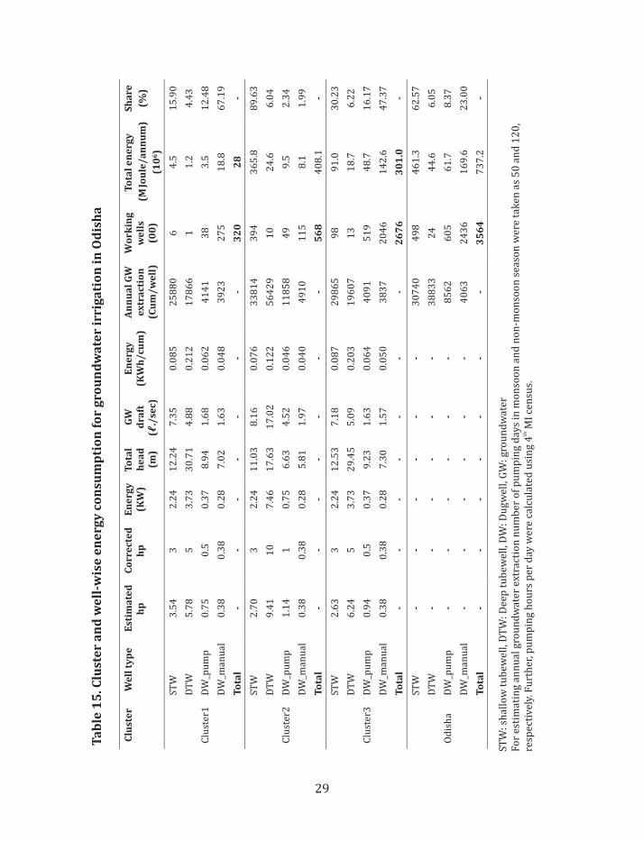
4.1.10.2. Estimation of energy consumed in groundwater irrigation in
Odisha
The energy consumption for groundwater irrigation depends on many factors such as
groundwater table depth, aquifer properties, type of well, horse power of the pump
(hp), pumping duration, etc. The energy consumption was estimated for different
type of well in each cluster separately. The weighted average of the horse power (hp)
27
was estimated as 3, 5, 0.5 and 0.38 for pumps with shallow wells, deep wells, dugwells
and man/animal energy, respectively in cluster1 (Table 15). In cluster2,
comparatively higher hp pump was used as compared to other clusters. But, due to
comparatively higher water table and favourable aquifer properties, estimated
discharge (lit/sec) in cluster2 was higher than other clusters.
3Consequently, energy used to extract per cubic meter groundwater (KWh/m ) was
comparatively less in cluster2 (alluvial/coastal belt) than other clusters (hard rock). 3Among different types of wells, energy consumption (KWH/m ) was highest in deep
tubewells followed by shallow tubewells, dugwells (pump) and dugwells
(man/animal) in all the clusters. The total energy consumption to extract 8groundwater annually (M Joule/annum) was estimated as 7.37 10 MJoule/annum in
8Odisha, 55 per cent (4.08 10 M Joule/annum) of which was consumed in cluster2.
Cluster1 and cluster3 consumed 4 per cent and 41 per cent of the total energy
consumed, respectively. Among the groundwater structures, shallow tubewells
constituted highest share (63%) in the total energy consumed followed by dugwells
(man/animal) in Odisha. However, this pattern varied across different clusters. In
cluster1 and cluster3, dugwells (man/animal) constituted predominant share in total
energy consumption, while in cluster2 shallow wells were the major consumer of
energy (90%).
At farm level, energy consumption will depend on the type of the crops grown and
their irrigation requirement. During kharif season, water requirement of many crops
are mainly fulfilled by rainfall. However, supplemental irrigation is needed during
long dry spell in few areas only. But during rabi and summer season, irrigation
requirement are mainly fulfilled through groundwater. In the present study, energy
requirement under different groundwater conditions for major crops grown in
Odisha has been estimated and presented in the Table16. The irrigation requirement
during rabi season (Nov-Jan) has been estimated based on potential evapo-
transpiration (PET) and crop coefficient values. PET for alluvial areas
(Jagatsinghpur) and hard rock area (khurda) has been calculated by FAO-56 method.
The estimated energy requirement by deep tubewells (120 m) was found to be about
24 times higher than shallow wells (5 m) but, deep tubewell can irrigate higher
command area.
28
Ta
ble
15
. Clu
ste
r a
nd
we
ll-w
ise
en
erg
y c
on
sum
pti
on
fo
r g
rou
nd
wa
ter
irri
ga
tio
n i
n O
dis
ha
Clu
ste
r
We
ll t
yp
e
Est
ima
ted
h
p Co
rre
cte
d
hp
En
erg
y
(KW
)
To
tal
he
ad
(m
)
GW
d
raft
(
/se
c)ℓ
.
En
erg
y
(KW
h/
cum
)
An
nu
al
GW
e
xtr
act
ion
(C
um
/w
ell
)
Wo
rkin
g
we
lls
(00
)
To
tal
en
erg
y
(MJo
ule
/a
nn
um
)
(10
6)
Sh
are
(%)
Clu
ster
1
STW
3
.54
3
2.2
4
12
.24
7
.35
0
.08
5
25
88
0
6
4.5
15
.90
DT
W
5.7
8
5
3.7
3
30
.71
4.8
8
0.2
12
17
86
6
1
1.2
4.4
3
DW
_pu
mp
0.7
5
0.5
0.3
7
8.9
4
1.6
8
0.0
62
41
41
38
3.5
12
.48
DW
_man
ual
0.3
8
0.3
8
0.2
8
7.0
2
1.6
3
0.0
48
39
23
27
5
18
.86
7.1
9
To
tal
-
-
-
-
-
-
-
32
0
28
-
Clu
ster
2
STW
2.7
0
3
2.2
4
11
.03
8.1
6
0.0
76
33
81
4
39
4
36
5.8
89
.63
DT
W
9.4
1
10
7.4
6
17
.63
17
.02
0.1
22
56
42
9
10
24
.66
.04
DW
_pu
mp
1.1
4
1
0.7
5
6.6
3
4.5
2
0.0
46
11
85
8
49
9.5
2.3
4
DW
_man
ual
0.3
8
0.3
8
0.2
8
5.8
1
1.9
7
0.0
40
49
10
11
5
8.1
1.9
9
To
tal
-
-
-
-
-
-
-
56
8
40
8.1
-
Clu
ster
3
STW
2.6
3
3
2.2
4
12
.53
7.1
8
0.0
87
29
86
5
98
91
.03
0.2
3
DT
W
6.2
4
5
3.7
3
29
.45
5.0
9
0.2
03
19
60
7
13
18
.76
.22
DW
_pu
mp
0.9
4
0.5
0.3
7
9.2
3
1.6
3
0.0
64
40
91
51
9
48
.71
6.1
7
DW
_man
ual
0.3
8
0.3
8
0.2
8
7.3
0
1.5
7
0.0
50
38
37
20
46
14
2.6
47
.37
To
tal
-
-
-
-
-
-
-
26
76
30
1.0
-
Od
ish
a
STW
-
-
-
-
-
-
30
74
0
49
8
46
1.3
62
.57
DT
W-
--
--
-3
88
33
24
44
.66
.05
DW
_pu
mp
--
--
--
85
62
60
56
1.7
8.3
7
DW
_man
ual
--
--
--
40
63
24
36
16
9.6
23
.00
To
tal
--
--
--
-3
56
47
37
.2-
STW
: sh
allo
w t
ub
ewel
l, D
TW
: Dee
p t
ub
ewel
l, D
W: D
ugw
ell,
GW
: gro
un
dw
ater
For
esti
mat
ing
ann
ual
gro
un
dw
ater
ext
ract
ion
nu
mb
er o
f p
um
pin
g d
ays
in m
on
soo
n a
nd
no
n-m
on
soo
n s
easo
n w
ere
tak
en a
s 5
0 a
nd
12
0,
thre
spec
tive
ly. F
urt
her
, pu
mp
ing
ho
urs
per
day
wer
e ca
lcu
late
d u
sin
g 4
MI
cen
sus.
29
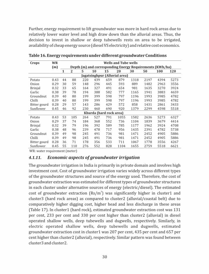
Further, energy requirement to lift groundwater was more in hard rock areas due to
relatively lower water level and high draw down than the alluvial areas. Thus, the
decision to invest in shallow or deep tubewells rests on area to be irrigated,
availability of cheap energy source (diesel VS electricity) and relative cost economics.
Table 16. Energy requirements under different groundwater Conditions
Crops WR (m)
Wells and Tube wells Depth (m) and corresponding Energy Requirements (KWh/ha)
4.1.11. Economic aspects of groundwater irrigation
The groundwater irrigation in India is primarily in private domain and involves high
investment cost. Cost of groundwater irrigation varies widely across different types
of the groundwater structures and source of the energy used. Therefore, the cost of
groundwater extraction was estimated for different types of groundwater structures
in each cluster under alternative sources of energy (electric/diesel). The estimated 3cost of groundwater extraction (Rs/m ) was significantly higher in cluster1 and
cluster3 (hard rock areas) as compared to cluster2 (alluvial/coastal belt) due to
comparatively higher digging cost, higher head and less discharge in these areas
(Table 17). In cluster1 (hard rock), estimated groundwater extraction cost was 131
per cent, 233 per cent and 330 per cent higher than cluster2 (alluvial) in diesel
operated shallow wells, deep tubewells and dugwells, respectively. Similarly, in
electric operated shallow wells, deep tubewells and dugwells, estimated
groundwater extraction cost in cluster1 was 207 per cent, 435 per cent and 657 per
cent higher than cluster2 (alluvial), respectively. Similar pattern was found between
cluster3 and cluster2.
30
Ta
ble
17
. Eco
no
mic
s o
f g
rou
nd
wa
ter
irri
ga
tio
n
E: E
lect
ric
pu
mp
, D
: Die
sel p
um
p1
.1
hp
=0
.74
6 K
W
2.
1H
p p
um
p c
on
sum
es a
bo
ut
25
0 m
l die
sel p
er h
ou
r3
. D
iese
l co
st @
Rs.
45
/lit
re, E
lect
ric
cost
@ R
s 1
.1/u
nit
(K
Wh
) 4
. Fo
r es
tim
atin
g an
nu
al g
rou
nd
wat
er e
xtra
ctio
n n
um
ber
of
pu
mp
ing
day
s in
mo
nso
on
an
d n
on
-mo
nso
on
sea
son
wer
e ta
ken
as
50
an
d 1
20
, th
resp
ecti
vely
. Fu
rth
er, p
um
pin
g h
ou
rs p
er d
ay w
ere
calc
ula
ted
usi
ng
4 M
I ce
nsu
s.
5.
Am
ort
izat
ion
was
do
ne
at 6
% r
ate
of
inte
rest
an
d a
vera
ge a
ge o
f w
ells
was
ass
um
ed a
s 1
5 y
ears
fo
r h
ard
ro
ck a
reas
an
d 2
0 y
ears
fo
r al
luv
ial
regi
on
. Ave
rage
age
of
pu
mp
was
ass
um
ed a
s 1
0 y
ears
6.
Sub
sid
y w
as e
stim
ated
@R
s. 1
0.9
4/l
iter
die
sel a
nd
Rs.
2.9
8/u
nit
(K
Wh
) o
f el
ectr
icit
y
Pa
rtic
ula
rs
En
erg
y
sou
rce
Clu
ste
r1
Clu
ste
r2
Clu
ste
r3S
TW
D
TW
D
W
ST
W
DT
W
DW
ST
WD
TW
DW
Ho
rse
po
wer
of
the
pu
mp
(h
p)
E
,
D
3
5
0.5
3
1
0
13
50
.5E
ner
gy (
KW
)1
E
,D
2
.24
3
.73
0
.37
2
.24
7
.46
0
.75
2.2
43
.73
0.3
7T
ota
l hea
d (
met
er)
E,D
12
.24
30
.71
8.9
4
11
.03
17
.63
6.6
31
2.5
32
9.4
59
.23
GW
dra
ft (
/sec
)ℓ
.
E,D
7.3
5
4.8
8
1.6
8
8.1
6
17
.02
4.5
27
.18
5.0
91
.63
Die
sel (
/ m
ℓ.
3)2
/ele
ctri
city
(K
Wh
/ m
3)
con
sum
pti
on
Ele
ctri
city
0.0
85
0.2
12
0.0
62
0.0
76
0.1
22
0.0
46
0.0
87
0.2
03
0.0
64
Die
sel
0.0
28
0.0
71
0.0
21
0.0
26
0.0
41
0.0
15
0.0
29
0.0
68
0.0
21
Co
st o
f en
ergy
(R
s/ m
3)3
Ele
ctri
city
0.0
9
0.2
3
0.0
7
0.0
8
0.1
3
0.0
50
.10
0.2
20
.07
Die
sel
1.2
8
3.2
0
0.9
3
1.1
5
1.8
4
0.6
91
.31
3.0
70
.96
Dig
gin
g C
ost
(0
00
, Rs)
E,D
10
0
30
0
90
50
15
0
30
10
03
00
90
Pu
mp
Co
st (
00
0, R
s)
E,D
15
30
8
15
55
10
15
30
8
An
nu
al M
ain
ten
ance
cost
(R
s)
Ele
ctri
city
15
0
30
0
80
15
0
55
0
10
01
50
30
08
0D
iese
l
75
0
15
00
40
0
75
0
27
50
50
07
50
15
00
40
0A
nn
ual
wat
er e
xtra
ctio
n (
m3/w
ell)
4
E,D
25
88
0
17
86
6
41
41
33
81
4
56
42
9
11
85
82
98
65
19
60
74
09
1
To
tal a
nn
ual
am
ort
ized
co
st (
Rs/
m3)
Ele
ctri
city
0.4
8
1.9
7
2.5
2
0.1
9
0.3
7
0.3
40
.42
1.8
02
.55
Die
sel
0.5
1
2.0
4
2.6
0
0.2
1
0.4
1
0.3
80
.44
1.8
62
.63
To
tal i
rrig
atio
n c
ost
(R
s/m
3)
Ele
ctri
city
0.5
8
2.2
1
2.5
9
0.2
8
0.5
1
0.3
90
.51
2.0
22
.62
Die
sel
1.7
85
.24
3.5
31
.36
2.2
51
.07
1.7
44
.93
3.5
9
Shar
e o
f en
ergy
in t
ota
lirr
igat
ion
co
st (
%)
Ele
ctri
city
16
.17
10
.57
2.6
33
0.2
12
6.3
71
2.7
91
8.5
51
1.0
72
.68
Die
sel
71
.61
61
.05
26
.40
84
.47
81
.64
64
.68
74
.87
62
.26
26
.78
To
tal e
lect
rici
ty (
KW
h/w
ell)
/die
sel (
/wel
l)
ℓ.
con
sum
pti
on
E
lect
rici
ty2
18
93
79
02
56
25
77
68
70
54
32
58
53
98
92
61
Die
sel
73
31
27
08
68
64
23
02
18
28
66
13
37
87
Per
wel
l su
bsi
dy
(R
s/w
ell)
Ele
ctri
city
65
22
11
29
57
62
76
79
20
47
41
61
97
70
21
18
87
77
7D
iese
l8
02
41
38
96
93
89
44
82
51
88
19
92
94
76
14
62
59
56
31
3Further, the groundwater extraction cost (Rs/m ) was significantly higher in diesel
operated pumps as compared to electric operated pumps. In cluster1, estimated
groundwater extraction cost in diesel operated shallow wells, deep tubewells and
dugwells was 309 per cent, 237 per cent and 136 per cent higher than electric
operated pumps, respectively. In cluster2, estimated groundwater extraction cost in
diesel operated shallow wells, deep tubewells and dugwells was 490 per cent, 443 per
cent and 271 per cent higher than electric operated pumps, respectively. Similarly, in
cluster3, estimated groundwater extraction cost in diesel operated shallow wells,
deep tubewells and dugwells was 490 per cent, 443 per cent and 271 per cent higher
than electric operated pumps, respectively. Significantly higher cost of groundwater
extraction in diesel operated pumps (than electric pump) was due to higher share of
diesel in total irrigation cost than electricity (Table 17). The share of diesel in total
irrigation cost was 72 per cent, 61 per cent and 26 per cent in cluster1, 84 per cent, 82
per cent and 65 per cent in cluster2 and 75 per cent, 62 per cent and 27 per cent in
cluster3 in shallow wells, deep tubewells and dugwells, respectively. On the other
hand, the share of electricity in total irrigation cost was 16 per cent, 11 per cent and 3
per cent in cluster1, 30 per cent, 26 per cent and 13 per cent in cluster2 and 19 per
cent, 12 per cent and 3 per cent in cluster3 in shallow wells, deep tubewells and
dugwells, respectively. Therefore, the impact of a unit increase in energy cost, a
common phenomenon now a days, on total irrigation cost will be much less in electric
operated wells than diesel pumps. However, in a situation which is plagued by poorly
developed power infrastructure, deficit and unreliable power supply, shifting from
diesel to electric energy is the most challenging task.
Presently, for irrigation/agriculture sector, being a special category both from
political and social ground, the Government is providing diesel as well as electricity at
subsidized rate. However, the impact of energy subsidy on the sustainability of the
water resources is a debatable issue among the researchers. On diesel, the
Government is providing subsidy of ₨.10.97 per liter as on February, 2012. Similarly,
the electricity tariff in Odisha is kept only at 110 paise per unit for LT connections and
100 paisa/unit for HT connections under a metered or pro-rata tariff system (OERC,
2011). However, the cost of electricity supply has been determined at 408.87 paise
per unit for 2011-12 and a cross subsidy of 298.87 paise per unit (408.87 – 110 paise
per unit) is paid to the farmers. Therefore, an increase in electricity tariff atleast by
217 paise per unit is required to reach the lower limit (408.78 – 20% =327.07) of the
prescribed electricity tariff (±20 per cent of the supply cost) by National Electricity
Policy (OERC, 2011).
32
The increase in electricity tariff will not only reduce the subsidy burden on
Government exchequer but also bring about efficiency in use of groundwater
resources due to positive marginal cost of the pumping (Kumar and Singh, 2001;
Saleth, R.M., 1997). But, tariff hike may also curtail the electricity demand and thereby
groundwater utilization. Due to the small share of electricity cost in total production
cost (Narayanmoorthy, A. 1997), tariff hike shall produce a meager impact on
groundwater withdrawal though there are divergent views on implications of tariff
hike on electricity demand and groundwater use (Kumar and Singh, 2001; Saleth,
R.M., 1997; De Fraiture and Perry, 2002) Kumar and Patel argued that net returns
from the well irrigated commands will be more elastic to adequacy and reliability of
irrigation water rather than the cost of energy. The positive impact of adequate and
quality electricity supply on farm economy will trickle down to well irrigators with
'man/animal' power (especially in hard rock areas) who will switch to electric pump
to cover higher command area and reduce drudgery.
The estimated groundwater extraction cost with the increased electricity tariff rate
(327 paise per unit for assessment year 2011-12) was lesser (30% to 135% in
cluster1, 117% to 207% in cluster2 and 30% to 149% in cluster3 depending upon
type of wells) than subsidized diesel operated wells. Hence, the farmers with the
diesel pump will naturally be shifting to electric pumps provided assured and quality
electricity supply is guaranteed. Additionally, if conducive product disposal
infrastructure (marketing, processing, cold storage, etc) is provided, the assured
irrigation will also motivate the farmers to diversify towards high value crops such as
vegetables, floriculture, etc which will accelerate the overall agricultural growth in
the state. It is worth noting that above mentioned benefits of electricity based
irrigation rest on the provision of assured and quality power supply and development
of favourable marketing infrastructure in the state. The part of the investment in
developing power and marketing infrastructure can be made through the increase in
power tariff and the removal of estimated annual subsidy per well (Table17).
Therefore, in the Odisha state, which is pioneer in electricity reforms in the country,
there is ample opportunity to harness the potential of groundwater resources
through suitable energy regulations for accelerated agricultural growth.
4.1.12. Inter-cluster variations in agricultural performance in Odisha
Odisha occupies 4.74 per cent of the geographical area and 3-4 per cent of the
agricultural and irrigated area of the country. The predominant agriculture and allied
sectors contribute about 30 per cent of the Odisha's GDP and provides livelihood to
about 60 per cent of the workforce. About 36 per cent of the total geographical area of
the state is put to agriculture use (Table 18) as compared to national average of 42 per
33
cent. Further, there exists wide variation in land use pattern in different regions of the
Odisha (Figure 11). In cluster1 and cluster3, 25 and 37 per cent of the total
geographical area is used for agriculture purpose, respectively as compared to 52 per
cent in cluster2. This is primarily because of predominance of forest area (46 % in
cluster1 and 39% in cluster3) in the former regions. The topography of the
agriculture land in the state is not uniform across the regions. 47, 28 and 24 per cent of
the cultivated area in Odisha is categorized as high, medium and low land with wide
inter-cluster variations (Figure 11). The cultivated land in cluster1 and cluster3 is
predominated by high land constituting 64 and 51 per cent of the total cultivated land,
respectively. On the other hand, cultivated land in cluster2 is predominated by low
land constituting 43 per cent of the total cultivated land. Varying topographic
characteristics along with the input use pattern and available infrastructure facilities
determine cropping pattern in a particular region.
Table 18. State of Agriculture in Odisha during TE 2008
Particulars Cluster1 Cluster2 Cluster3 Odisha
Geographical area (000, ha) 3808 2093 9697 15571
Net Sown area (000, ha) 953 1080 3616 5649 Agriculture coverage (%) 25.02 51.58 37.29 36.14
Groundwater Development (%) 14.23 42.90 24.37 26.14
Fertilizer Consumption (Kg/ha) 39 75 48 54
Agriculture Purpose (%)Share of Power Consumption for - - - 1.30
Average paddy yield (kg/ha) 2067 2320 2336 2317Agriculture Development Index (%)* 22.93 62.78 36.96 40.18
Agriculture development index has been estimated using agriculture coverage, cropping intensity, irrigation coverage, fertilizer consumption, groundwater development and paddy yieldData source: Directorate of Economics and Statistics, Government of Odisha
The Odisha's agriculture is primarily rainfed (only 35.62% irrigation coverage) and
dominated by paddy-fallow/pulses copping pattern. The paddy and pulses occupied
67 per cent and 50 per cent of the kharif and rabi cropped area, respectively in
triennium ending (TE) 2008-09 (Figure 12). Paddy was the predominant cereal crop
constituting 91 per cent of the total cereals area in the state TE 2008-09 (Table 19). In
cluster1 and cluster3, cropping pattern was found to be more diversified than in
34
cluster2. In cluster2, 91 per cent of the kharif and 53 per cent of the rabi cropped area
was found to be occupied by cereals (paddy constituted 99% of total cereals area) and
pulses in TE 2008-09, respectively. The low and medium land topography (83% of
total cultivated area) in cluster2 might have contributed significantly for the
dominance of paddy in the cropping pattern because of suitability of paddy (95 per
cent of the low land and 86 per cent of the medium land was occupied with paddy) in
these areas (Figure 13). Interestingly, in 43 per cent (0.97 lakh ha) of the total high
land (2.25 lakh ha) in cluster2, paddy was cultivated in TE 2008-09 which can be
substituted by the non-paddy crops. In cluster1, comparatively less area is cultivated
under cereals (71%) than cluster2 in kharif season and paddy occupied 71 % of the
total cereals areas. About 20 per cent of the kharif cropped area was occupied by
pulses and oilseeds in TE 2008-09. The oilseeds and pulses must have been
cultivated in high land (61% of total cultivated land) in cluster2. Further, 99, 76 and
35 per cent of the total low (1.37 lakh ha), medium (2.33 lakh ha) and high (6.72 lakh
ha) land in kharif season was occupied with paddy, respectively. Therefore, paddy
occupied high land area (35% or 2.34 lakh ha) in cluster1 can be substituted by the
non-paddy crops. In the rabi season, 40 per cent of the total cultivated area was
constituted by pulses followed by oilseeds (22%) and vegetables (19%) in TE 2008-
09. It is to be noted that the share of vegetables in total rabi cropped area was highest
in cluster1 as compared to other regions. Thus, the promotion of vegetables
cultivation in cluster1 along with the micro-irrigation system (feasible technology for
low discharge rate aquifers) appears the promising target. Similarly, in cluster3,
vegetable cultivation can be promoted by diverting about 35 per cent (7.12 lakh ha) of
the high land area which is presently been cultivated under paddy. Thus, there exists
scope for diversification in paddy occupied 10.43 lakh ha (36% of the total high land)
area in Odisha by developing irrigation facilities (both surface and groundwater),
adequate input supply and efficient marketing infrastructure. Cluster1, cluster2 and
· It is prudent to invest in providing quality electricity for pumping at higher
prices than subsidizing electricity for agriculture as removing electricity
subsidy would increase the irrigation cost only by 3-16 per cent in cluste1,
13-30 per cent in cluster2 and 3-19 per cent in cluster3 depending upon the
type of wells used. This increase will be much lower than the irrigation cost
using even subsidized diesel. Consequently, if assured and quality electricity
is guaranteed, irrigators with diesel pump will switch to electrical energy to
maximize the net profit. The part of the investment needed for creating such
infrastructure can be met by removal of energy (electricity/diesel) subsidy.
· There exists scope for diversification in paddy occupied 10.43 lakh ha (36%
of the total high land) area in Odisha. The scope for diversification is more in
the regions (cluster1 and cluster3) witnessing poor agricultural
performance. Sustainable groundwater development activities along with
adequate input supply and efficient marketing infrastructure would go a long
way to improve the agricultural performance in the state.
40
4.2. Summary and conclusion
Odisha's agriculture sector is characterized as low input-low productive with high
risk and regional inequality. The groundwater development bears a positive
relationship with the agricultural income and as most of the ultimate irrigation
potential (UIP) from groundwater in Odisha remains unutilized due to under-
development of groundwater resources, its sustainable development will accelerate
the agriculture growth in the state. However, the groundwater resources in Odisha
are suffering from dual problem of its under-development as well under-utilization
of already created irrigation potential. The under-development of groundwater in
the state is primarily due to predominance of hard-rock geology which restricts its
development due to its aquifer properties. Implementation of suitable recharge
activities using scientific tools and investigations in these areas would improve the
well yield and subsequently groundwater draft for irrigation. On the other hand,
groundwater exploitation in comparatively better developed alluvial/coastal areas
needs precautions with respect to sea water intrusion. The regulation of pumping
depth, horse power (hp) and pumping hours within the safe limit and its strict
monitoring at local governance level in coastal areas is essential to avoid negative
externalities of groundwater development. The under-utilization of already created
irrigation potential not only lead to loss of financial resources but also opportunity to
improve agricultural productivity through advantages of assured irrigation. Non-
functioning of wells was one of the important factors of poor utilization of created
potential. These defunct wells can be repaired, reinstalled and maintained to
improve irrigation infrastructure which would involve much less investment than
creating new structures in the state. Mass-scale non-functionality of deep wells
(primarily owned by Government) sets an urgent need of transferring their
ownership towards better performing Pani-Panchayat/water users' association. The energy use pattern, which bears a direct relationship with groundwater
development, exhibited regional variations in the state. In the hard rock region,
'man/animal' power was the dominant energy source (because of predominance of
dugwells), while diesel emerged as a major energy source in the alluvial/coastal
areas. Inspite of technological superiority and cheap operational and maintenance of
electric pumps over diesel pumps, farmers are forced to use diesel operated pumps
due to poor power infrastructure and unreliable electricity supply for irrigation
purpose. The cost of groundwater extraction using diesel is much higher than
electricity and the increased groundwater extraction cost at higher electricity tariff
(if electricity subsidy is removed) will be lesser than using diesel even at subsidized
rate. Consequently, if assured and quality electricity is guaranteed, irrigators with
diesel pump will switch to electrical energy to maximize the net profit. The positive
41
impact of assured and reliable electricity will also trickle down to irrigators using
'man/animal' power to switch to electric pump in the hope of higher irrigation
coverage and reduced drudgery. Additionally, if conducive product disposal
infrastructure (marketing, processing, cold storage, etc) is provided, the assured
irrigation will motivate the farmers to diversify towards high value crops such as
vegetables, floriculture, etc which will accelerate the overall agricultural growth in
the state. The scope of diversification is more in hard rock regions of the state.
However, realization of the above mentioned benefits rests on the condition of
assured and quality electric supply for irrigation and conducive market
infrastructure in the state. The part of the investment needed for creating such
infrastructure can be met by removal of electric as well diesel subsidy. Therefore, in
the Odisha state, which is pioneer in electricity reforms in the country, there is ample
opportunity to harness the potential of groundwater resources through suitable
technological interventions and energy regulations for accelerated agricultural
growth.
References:
Briscoe, J. and Malik, R.P.S. India's Water Economy: Bracing for a Turbulent Future. The World Bank, Oxford University Press, New Delhi, 2006.
CGWB, Groundwater Scenario of India, Ministry of Water Resources, Government of India, 2010.
De Fraiture, C., Perry, C. Why is the irrigation water demand curve inelastic at low price ranges? Paper presented at International conference on: Irrigation water Policies: Micro and macro considerations. Jointly organized by Worldbank and Government of Morocco. Agadir, Morocco, June 15-17, 2002.
Government of Odisha, Economic Survey, 2009-10, Planning and Coordination Department, Directorate of Economics and Statistics, 2010.
Jeet, I., Groundwater Resources of India: Occurrence, Utilization and Management, New Delhi, Mittal Publications, 2005.
Kumar, Dinesh, Demand Management in the Face of Growing Water Scarcity and Conflicts in India: Institutional and Policy Alternatives for Future. In Chopra, Kanchan, Rao, Hanumantha, C.H. and Sengupta, Ramprasad (Eds.) Water Resources and Sustainable Livelihoods and Eco-System Services, Concept Publishing Company, New Delhi, 2003, 97-131.
A. Narayana Moorthy (2008), “Losers and gainers of groundwater irrigation development: an empirical study from peninsular India”, Annual Report, 2008, IWMI water policy research prgramme , Phase II: 2006-2010.
Ballabh Vishwa, K Chowdhary, Sushil Pandey and Sudhakar Mishra (2002). 'Groundwater Development and Agricultural Production: A Comparative Study of Eastern Uttar Pradesh, Bihar and West Bengal'. IWMI-Tata Water Policy Research Program, Anand
Dhawan, B.D. (1982). 'Development of Tubewell Irrigation in India'. Agricole Publishing Academy, New Delhi.
42
Kumar, M.D. and Singh, O.P., market instruments for demand management in the face of growing scarcity and overuse of water in India. Water Policy 5(3), 86-102, 2001
Kumar, M.D., Patel, P.J., Depleting buffer and farmers response: study of villages in Kheralu, Mehsana, Gujarat. In: Moench, M. (Ed.), Electricity prices: A tool for Groundwater management in Inda? VIKSAT- Natural Heritage Institute, Ahmedabad.
Malik, R.P.S., Energy regulations as a demand management Option: potentials, problems, and prospects, In Saleth, R.M. (Ed), Strategic analyses of the National River Linking Project (NRLP) of India, Series 3. Promoting Irrigation Demand management in India: Potentials, Problems and Prospects. International Water Management Institute, Colombo, Sri Lanka, 2008, 71-92.
OERC, Annual Report, 2010-11, Orissa Electricity Regulatory Commission, Government of Odisha, 2011.
Rodell, M, Isabella Velicogna and James S Famiglietti (2009): “Satellite-based Estimates of Groundwater Depletion in India”, Nature, Vol 460, 20 August.
stRosegrant M., Water resources in 21 Century: Challenges and implications for action.
Food, agriculture and environment Discussion paper 20. IFPRI, Washington DC., 1997.
Saleth, R. M., Power tariff policy for groundwater regulation: Efficiency, Equity and sustainability. Artha Vijnana 39 (3), 312-322, 1997.
Sethi, L. N., Sudhindra N. Panda and Manoj K. Nayak (2006), “ Optimal crop planning and water resources allocation in a coastal groundwater basin, Orissa, India”, Agricultural Water Management, 83, pp. 209-220.
Shankar, P.S.V, H. Kulkarni, S.R. Krishna (2011), India's groundwater Challenge and the way forward, Economic & Political Weekly, January 8, Vol xlvi 38 no 2.
Sharma, K.D. (2009), “Groundwater management for food security” , current Science, Vol. 96, No. 11, 10 June, 2009, pp. 1444-1447.
Singh, O.P. (2008), “
Srivastava, N.S.L. Animate Energy in Agriculture. Publication on Invited Papers International Conference on Managing Natural Resources for Sustainable Agricultural. Production in the 21st Century, held at New Delhi during February 14-18, 2000, 466-477, 2002.
Swain, M., Mrutyunjay, Swain and D.K. Das, (2009), “ regional disparity in agricultural development in Orissa in the pre and post reform period”, Social Change, vol. 39 no.2 , pp. 195-215.
Impact of energy pricing and supply regulation on irrigated agriculture: A comparative analysis from water rich and water scarce regions of India”, Annual Report, 2008, IWMI water policy research programme , Phase II: 2006-2010.