C Fermi National Accelerator Laboratory FERMILAB-™·1851 Groundwater Migration of Radionuclides at Fermilab A.J. Malensek, A.A. Wehmann, A.J. Elwyn, K.J. Moss and P.M. Kesich Fermi National Accelerator Laboratory P.O. Box 500, Batavia, Illinois 60510 August 1993 :Q: Operated by Universities Research Association Inc. under Contract No. DE-AC02-76CH03000 with the United States Department of Energy
Transcript
C Fermi National Accelerator Laboratory
FERMILAB-™·1851
Groundwater Migration of Radionuclides at Fermilab
Fermi National Accelerator Laboratory P.O. Box 500, Batavia, Illinois 60510
August 1993
:Q: Operated by Universities Research Association Inc. under Contract No. DE-AC02-76CH03000 with the United States Department of Energy
Disclaimer
This report was prepared as an account of work sponsored by an agency of the United States Government. Neither the United States Government nor any agency thereof, nor any of their employees, makes any warranty, express or implied, or assumes any legal liability or responsibility for the accuracy, completeness, or usefulness of any information, apparatus, product, or process disclosed, or represents that its use would not infringe privately owned rights. Reference herein to any specific commercial product, process, or service by trade name, trademark, manufacturer, or otherwise, does not necessarily constitute or imply its endorsement, recommendation, or favoring by the United States Government or any agency thereof The views and opinions of authors expressed herein do not necessarily state or reflect those of the United States Government or any agency thereof.
Groundwater Migration of at Fermilab
Radionuclides
A. J. Malensek, A. A. Wehmann, A. J. Elwyn, K. J. Moss, and P. M. Kesich
September 20, 1993
Abstract
The simple Single Resident Well (SRW) Model has been used to calculate groundwater movement since Fermilab's inception. A new Concentration Model is proposed which is more realistic and takes advantage of computer modeling that has been developed for the siting of landfills. Site geologic and hydrologic data were given to a consultant who made the migration calculations from an initial concentration that was based upon our knowledge of the radioactivity leached out of the soil. The various components of the new Model are discussed, and numerical examples are given and compared with DOE/EPA limits.
1
2
Table of Contents
1.0 Introduction
2.0 Water Movement 2. 1 The Zones 2. 2 Unsaturated Zone and the Capillary Fringe 2. 3 Saturated Zone 2.4 Fractures
3.0 CASIM
4.0 SRW Model
5. 0 Concentration Model 5. 1 The Philosophy 5 .2 The 99% Solution 5.3 Average Star Density 5 .4 Activation 5.5 Leaching 5.6 Propagation
Woodward-Clyde Consultants Loss Points and Drinking Water Wells Mathematical Models Initial Conditions Input Data The Vertical Velocity in the Glacial Till Calculations: Reduction Factor Results Regulations and the Annual Limits Application of Results Numerical Examples
9 .0 Acknowledgments
10.0 Appendices 10 .1 Hydraulic Conductivity vs. Pressure 10.2 Travel Through the Unsaturated Zone 10. 3 Fracture Flow in Dolomite 10.4 Build-up to Saturation 10.5 Numerical Examples
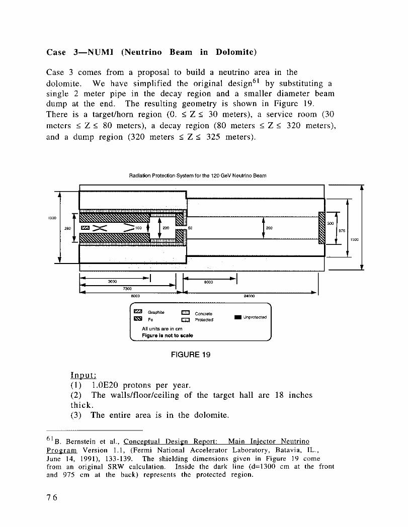
10.5.1 Target followed by a long buried pipe 10.5.2 Typical enclosure + dump. R=4', Z=20' 10.5.3 Neutrino beam in dolomite
11.0 References
3
1 Introduction
Fermilab is a research laboratory consisting of a senes of large particle accelerators known as the Linac, Booster, Main Ring and the Tevatron. Beams of elementary charged particles are accelerated m these machines, and reach an energy of many hundred billion electron volts. 1 These high energy particles are made to collide either within the Tevatron itself (Collider Mode), or the particles are extracted from the Tevatron and directed onto external stationary targets (Fixed Target Mode). Radioactivation of soil is caused by particles produced during accelerator operations. Soil activation is highest outside locations where a particle beam strikes physical objects (hereinafter referred to as "sources"). In the region (called the "protected" region), considerable shielding such as steel and concrete is placed around a source to contain the vast majority of secondary and subsequent generations of particles. In the soil outside the shielding (called the "unprotected" region) there commonly exists groundwater. The natural migration of this groundwater carries the radioactivity beyond the area of activation toward aquifers used for drinking water.
The degree to which radionuclides migrate impacts on the design-controlling the amount of steel, concrete, and other shielding-at source locations. During the years that Fermilab has been in existence, a number of studies have addressed this particular concern. 2 Designers of new facilities have expressed concern that the
1 Protons and anti-protons; the anti-protons are produced by extracting protons from the Main Ring and colliding them in a special target. From the target they are collected and "cooled" in Fermilab's Anti-Proton Source. They are reintroduced into the Main Ring for acceleration and transferred to the Tevatron, where they are further accelerated and brought into collision with the proton beam at two collision points in "collider mode." 2 A seminal document in the series is TM-816, "Soil Activation Calculations for the Anti-Proton Target Area", Peter J. Golian, Sept. 14, 1978. Another document is TM-945, "Soil Activation Calculations for the Proposed Neutrino Front Hall'', J.D. Cossairt, Jan. 15, 1980. Groundwater activation is also discussed in the Fermilab Radiological Control Manual. It gives the "Derived Concentration Guides" (DCG) for Accelerator Produced Radionuclides in Water, in Table 3-1 of Chapter 3. Studies of groundwater activation (TM-816 cites Borak) have determined that the radionuclides that are relevant to possible contamination
of drinking water coming from local aquifers are 3H (Tritium) and 22 Na . For these the DCG values are 20 and 0.4 picoCuries/milliliter, respectively. We use these values in the remainder of this report.
4
current SRW Model used to specify source shielding requirements is in need of revision. 3 In January 1992 the Research Di vision and the ES&H Section contributed personnel to a joint committee charged with re-examining the methodology of calculating the radionuclide production and transport in groundwater in the vicinity of source points. The committee was asked to engage the services of a consulting firm to model the movement of radionuclides in the groundwater. 4 The consulting firm selected, Woodward-Clyde Consultants, has extensive experience and expertise in groundwater studies.
The method presently used at Fermilab to calculate groundwater activation (the SRW model) employs the computer program CASIM5 to calculate nuclear "stars" 6 per incident proton m the unprotected region. The CASIM results (which are expressed m
stars/cm 3 per proton) are multiplied by the number of incident protons and integrated over the entire unprotected volume to give the total number of stars produced in the soil. The amount of activity produced is directly proportional to the number of stars. The amount of activity for each radionuclide reaching the aquifer depends on the production, leachability, and travel time downwards (decay factor). Upon reaching the elevation of the aquifer, no further travel time is assumed. The concentration in drinking water is then
3we refer to the current model as the SRW model (Single Resident Well). One designer wrote an extensive Technical Memo on this point. It is Fermilab TM-838, "Aquifer Dilution Factors of Ground Water Activity Produced around Fermilab Targets and Dumps", A.M. Jonckheere, Dec. 1,1978. S. Baker drafted a TM in response, but never had it published in the TM system. It can be found in the files of the ES&H Section. 4Consulting firms are routinely engaged by industries and communities when there are concerns over contaminants penetrating into the drinking water. The Woodward-Clyde report will also serve to provide quantitative results that may prove useful in DOE National Environmental Policy Act (NEPA) reviews for new projects or modifications to existing facilities. Depending on the scope of the project, permits may be required by the State of Illinois and/or other Federal agencies before construction can begin. 5 A. Van Ginneken, "CASIM-Program to Simulate Transport of Hadronic Cascades in Bulk Matter". (Fermi National Accelerator Laboratory, Batavia, IL., Internal Report FN-272, 1975); also A. Van Ginneken and M. Awschalom. "Hadronic Cascades, Shielding, Energy Deposition", High Energy Particle Interactions in Large Tan;:ets, , Vol. I. (Fermi National Accelerator Laboratory, Batavia, IL., 1975) 6The term "star" comes from early cosmic ray observations in which high energy interactions with large multiplicities of secondary particles looked like "pointed stars" in detectors such as emulsions, bubble chambers, etc.
5
calculated by taking the act1v1ty entering the aquifer in one year, and dividing it by a quantity of water equal to 40 gallons per day times 365 days 7 .
This existing methodology is contrasted with a new "concentration" model which is more realistic and utilizes groundwater modeling. The new model employs CASIM results to determine the peak star density in the unprotected soil. Using cylindrical coordinates, the peak star density is averaged over a soil volume defined to have its limits at 99% of the star density in both the r and z dimensions (hereinafter referred to as the "99% volume" 8 ). An initial concentration is obtained by taking the activity in the "99% volume" of soil and dividing it by a volume of water that is sufficient to leach out 99% of the activity in the soil. A consultant's model of groundwater migration calculates the change m concentration after it moves vertically to the dolomite aquifer, then horizontally to the nearest well or site boundary.
To assist the reader, the report is separated into sections. Section 2, Water Movement, qualitatively presents a brief overview of water moving through unsaturated and saturated media. Section 3, CASIM, describes the computer program which is used to calculate how much radioactivity is deposited in the soil. Section 4, SR W Model, summarizes the Single Resident Well Model which is presently used to calculate groundwater migration. Section 5, Concentration Model, gives the details of the proposed new model. Section 6, Protected and Unprotected Regions, discusses the guidelines used for drawing the line between regions where water is controlled from those where it can migrate to the aquifer. Section 7, Report of Woodward-Clyde Consultants, discusses the technical results and the input that went into calculating the change in concentration as groundwater moves through the glacial till and the dolomite. Section 8, Sum ma ry, presents the major points and states the recommendations of Woodward-Clyde for decreasing the range of the modeling results.
7 This is the amount considered to be drought condition usage in a private well. The sum of all the leached radionuclides in the unprotected region for a given beam line gets transported to one well, where it mixes with the daily volume of water that is consumed by a single resident. See Gollon's TM-816 for further discussion. 8Using as the limits the points at which the star density decreases to 1 % of its maximum value in the r and z dimensions, the activity in this volume is actually about 93% of the total; 99% in z and 94% in r (see Section 5.3).
6
2 Water Movement
2 . 1 The Zones
From the standpoint of water content, the subsurface can be divided into (1) an unsaturated zone, (2) a saturated zone, and (3) a capillary fringe between them (see Figure 1). The unsaturated zone extends from the land surface to the top of the water table and includes those sediments where the soil pore pressure is less than atmospheric. The water table is the top surface of the saturated zone at which the pore pressure is atmospheric.
Ground Surface
Unsaturated Zone
Water Table
Figure I-Groundwater Zones
The capillary fringe has pores that are saturated, but the pressure is less than atmospheric. This zone is immediately above the water table where water is drawn upward by capillary attraction. The capillary rise is inversely proportional to the grain size of the particular soil type. For example, the capillary fringe in silt will be larger (have greater depth) than in sand.
7
The saturated zone begins at the water table and as the name suggests, the soil pores are completely filled with water and the fluid pressure is greater than atmospheric. The physical processes controlling the flow of water through saturated porous rock or soil are well understood. Darcy's equation9 has been investigated in the laboratory and is known to yield good predictions of head and flow under a wide range of conditions. Cases where Darcy's equation is not adequate have been reasonably well delineated. 10 Because the form of the equations are typical of a wide variety of physical problems and have been studied extensively in many contexts, many powerful tools of mathematical analysis are applicable. A number of computer codes are readily available and are accepted by the US EPA. Proper use of the numerical and analytic codes, however, still requires considerable training and experience by hydrologists and geologists. The focus of this report is on migration through the saturated zone.
2. 2 The Unsaturated Zone
Because of the complex phenomena taking place in the unsaturated zone, the overall problem is simplified by assuming the groundwater migrates instantaneously into the saturated zone without dilution. Appendix B shows that water falling on an "open, level field" spends only a matter of days traveling through the unsaturated zone and the capillary fringe. A discussion of the unsaturated zone is presented to highlight what makes calculations so difficult and the answers so hard to justify.
Soils near the ground surface are seldom saturated. Their voids are usually only partially filled with water, the remainder of the pore space being taken up by air. Qualitatively, unsaturated water flow begins with water falling on the surface. The rate of flow in the soil is controlled by the water input rate and the existing soilwater conditions. In the early stages when the soil is "dry" the water
9Darcy reported on experiments he did to analyze water flowing through sand. His results were generalized into the empirical law that now bears his name. It states that the flow rate across an area is equal to the hydraulic conductivity of the material, times the hydraulic gradient across it. In its simplest one dimensional form, the discharge rate is called the seepage velocity and is
Q Jh written as - = v = -K-
A x Jx !OR. Allen Freeze and John A. Cherry, Groundwater, (Englewood Cliffs, New Jersey: Prentice-Hall Inc., 1979), 69-75.
8
input is the dominant factor, but in later stages as the soil takes on more water and the wetting front penetrates deeper, the potential gradient driving the water flow decreases. After some time the water begins to pond at the surface and is lost as runoff. When water input at the surface ceases, the water content in the soil decreases as water begins to redistribute itself deeper. This is commonly called percolation and results in water movement from the unsaturated zone through the capillary fringe into the saturated zone. Finally, after redistribution, any change in water content comes about by losses due to plant uptake (evapotranspiration). This action continues until the next time water falls on the surface (e.g., rainfall, irrigation). Although we are concerned with migration to the aquifer, we point out that tritium shows up in vegetation growing in radioactive soil as groundwater is picked up by the root system. 11 A study 12 of evapotranspiration at Sheffield, Illinois where the entire site is covered by grass, indicates that total precipitation is partitioned approximately in the following way: (a) evapotranspiration-70%, (b) surface runoff-25%, and (c) transport into the aquifer-5%.
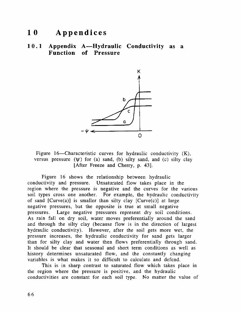
The unsaturated zone and capillary fringe are much more complex than the saturated zone where the hydraulic conductivity and the moisture content are constant. Both variables in the unsaturated zone are functions of pressure. These functional relationships are not easily obtained, they are site specific, and they are not single-valued but have hysteresis-type characteristics (see Appendix A). As a result, the behavior of groundwater may act opposite to that in the saturated zone, and one can actually have groundwater move preferentially through clay rather than sand.
This phenomena has been experimentally verified at Sheffield, Illinois-a low-level radioactive waste disposal site in northern Illinois. The report states "the hydraulic conductivity of the sand is much less than the adjacent finer grained sediments so the sand would impede the downward flow of water, possibly making it easier for water to move around the sand than through it". 1 3
11 M. Peter de Vries and Richard W. Healy, "Results of Hydrologic Research at a Low-Level Radioactive-Waste Disposal Site Near Sheffield, Illinois", US Geological Survey Report 88-318, ed. Barbara J. Ryan, (Urbana, IL., 1989), 29-36. 12J. B. Foster et al., "Hydrogeology of a Low-Level Radioactive Waste Disposal Site near Sheffield, Illinois", US Geological Survey Report 83-4125, (Urbana, IL., 1984), 34. 13 Ibid., 16, 61-62.
9
Given the complex nature of the variables, the unsaturated form of the governing equation is highly non-linear and difficult to solve numerically .14 Finally, there is a vast difference between the time and space scales. The unsaturated zone requires steps on the order of seconds and centimeters whereas the saturated zone may require years and kilometers. 15 By showing that water passes quickly into the saturated zone, we will be conservative by taking no credit for decay or dilution in the unsaturated zone and the capillary fringe. More importantly, no highly complex and detailed calculations will have to be made which require data that are not available, and are difficult to obtain. Two cases are cited in Appendix B to support the claim that water travels quickly through the unsaturated zone and the capillary fringe.
2. 3 The Saturated Zone
Saturated continuum flow models have been investigated extensively and are quite well understood, both theoretically and experimentally. The mathematical statements of the fundamental physical laws governing general fluid motion-conservation of mass, momentum, and energy-which are collectively known as the NavierStokes equations 16 are universally accepted. More important, the simplification of these equations lead to Darcy's law for fully saturated flow through a porous medium. For fluid flow, the process responsible for moving fluid mass into and out of a volume element is simply flow in response to a potential gradient. In its simplest form, the Darcy equation states that the mean velocity of water flowing through a porous medium is related to the product of the hydraulic gradient and a constant of proportionality called the hydraulic conductivity. For any site, it is impractical to have a complete and continuous set of data for the entire geology along with pressure heads, because monitoring wells and boreholes are discrete and finite in number. Our study does not seek an exact knowledge of the site geology/hydrology; rather, the local geology is sampled over a wide region and that data is used to infer the contents in the
14 Mary P. Anderson and William W. Woessner, Applied Groundwater Modeling, (San Diego, California: Academic Press, Inc., 1992), 323. 15 Ibid., 324. 16The Navier-Stokes equation for a Newtonian incompressible fluid is widely known in the study of fluid mechanics. It is applied to the flow of water through porous media by balancing the average momentum, subject to boundary conditions on the solid/fluid interface. See [Bear, p. 17, 42].
1 0
unsampled volume. The inference is based on the experience and best judgment of geologists and hydrologists. This approach allows us to take advantage of the current wealth of knowledge gained from their modeling experience.
The basic statement of groundwater flow is a second order differential equation, modified to incorporate two crucial processesdispersion and radioactive decay .17 Dispersion occurs because of the mechanical mixing of fluids. Qualitatively, it has a similar effect to turbulence in surface water dynamics. As contaminated water flows through a porous medium, it will mix with non-contaminated water.
The uniqueness of the solution to the differential equation for any particular groundwater flow problem involves boundary conditions. Often the boundaries correspond to physical boundaries in the environment along with conditions that are known or can be estimated by the use of data. In other situations, model boundaries must be defined on the basis of practicality-physical boundaries that are unknown or are at great distances from the region of interest. In either case, boundary condition specification is extremely important and requires the understanding of the mathematical role of boundary conditions as well as the hydrogeologic environment.
2. 4 Fractures
The saturated zone consists of glacial till sediments underlain by dolomite and shale formations respectively. The bedrock system underlying Fermilab is described well in hydrogeological terms by Zeizel. 18 The bedrock aquifer immediately underlying the glacial till on the Fermilab site is formed of Silurian age rocks that are principally dolomite. This is underlain by shale that separates the dolomite aquifer from deeper aquifers. The movement of water in the dolomite aquifer is mostly horizontal. Its direction is generally southeast, except where affected by well pumpage.
Dolomite very often develops a secondary porosity that is the result of (1) fracturing, (2) weathering, and (3) enlargement of
1 7 I . . 1 d' . 1 n its s1mp est one 1mens10na form it can be written as
D J2c -v JC -AC= JC x Jx2 x Jx Jt
D is the dispersion coefficient; C is the concentration; v is the seepage velocity; A. is the decay constant(reciprocal of the mean lifetime). 18 A. J. Ziezel, et. al., Ground-Water Resources of DuPa~e County. Illinois, Cooperative Ground-Water Report 2, Illinois State Water Survey and Illinois State Geological Survey, (Urbana, IL, 1962), 13-26.
1 1
openings by the flow of groundwater with the minerals making up the rock. Dolomite is limestone that has been altered by chemical replacement of some of its calcium by magnesium. This serves to make it significantly tougher than limestone. Limestone is typically an accumulation of organisms which precipitate CaC03 to make their
shells. Both limestone and dolomite are subject to redissolution in water. In such soluble rock, conduit flow can develop as original fracture systems are enlarged by solution.
Two examples of channeling in the dolomite were given to us by R. Sasman, IL State Water Survey, (retired). (See Appendix C for details). The first example in DuPage County involved a situation where contamination entered a community well in Darien, Illinois. Upon investigation, a nearby "abandoned" well was found with its casing terminated several feet below ground level. Pump tests using a tracer showed that contaminated surface water entered the pit of the "abandoned" well, flowed down its casing and then into the community well via fractures between the two wells. A private well was located between the community well and the "abandoned" well, but there was no evidence that any fractures were connected to it.
The second example involved the observation of three wells in southern Cook County while pumping on a fourth. Along the surface, the distance from the pumped well to the other three were 380 feet, 500 feet, and 700 feet. The well 700 feet away had a significantly larger drawdown (the difference between the static water level and the level while pumping) than the two others that were much closer. Normally, in a porous medium, the nearer the well, the larger the drawdown.
Sasman concludes: "Such variations in the effects of pumping in the dolomite are not uncommon. Water in this formation moves through cracks and crevices of undetermined length and direction. No method has been devised to determine precisely the extent and location of these fractures".
In the Woodward-Clyde Consultant's analysis and report, the Silurian Dolomite has been considered to be non-fractured. The flow calculations are done by equating the dolomite to a porous medium. The book Ground Water Models, Scientific and Regulatory Applications 19contains guidance on the applicability of this approach. A few quotations from it will be insightful: "In most practical problems involving saturated flow in fractured media, there
19National Research Council, Ground Water Models. Scientific and Re~ulatory Applications, (Washington, D. C.: National Academy Press, 1990), 107.
1 2
has never been much hesitation in applying continuum-type models . . . . The question remains, however, as to how realistically such models account for the fractured flow processes. Experience from the petroleum industry does suggest that in some cases more sophisticated flow formulations (e.g. dual-porosity models) will be required".
1 3
3 CA SIM
Hadronic cascades develop within the source and those particles which leak through the shielding around the source activate the surrounding material. The program known as CASIM simulates this process. It follows the average development of internuclear cascades when high energy particles are incident on large targets of arbitrary geometry and composition. The program computes nuclear interaction densities (called star densities) as a function of location throughout the materials. As will become apparent in several of the following sections, the star density (S) obtained from CASIM, together with a production cross-section, is used to calculate the
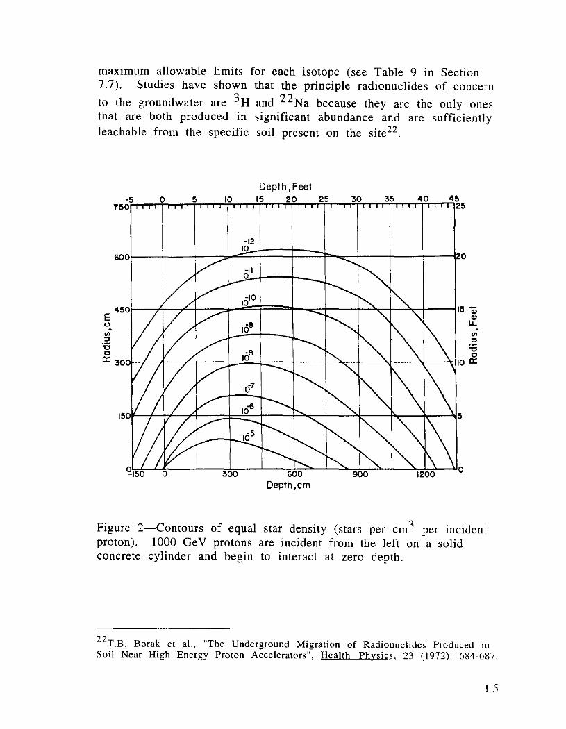
amount of 3H or 22Na produced in soil. Figure 2 shows CASIM results for the distribution of star densities as a function of position for 1000 GeV protons striking a solid concrete cylinder. The radiation pattern is cylindrically symmetric in the radial direction, but builds up and then diminishes in the direction along the beam. Calculations compare favorably with data for a wide variety of beam
loss and shielding geometries. 20•2 1
Figure 3 shows a typical situation, where the source is located inside an underground enclosure. Surrounding the source are two regions-a protected region and an unprotected region. The protected region is "sized" transversely and longitudinally to absorb most of the hadronic cascade. Radioactivation is controlled in the protected region because it is confined and remains localized by containment within a boundary. This is usually accomplished with a combination of steel and concrete inside the underground enclosures, nonpermeable liners, sump pumps, etc. The unprotected region is one outside the protected region where the radionuclides can freely migrate in three dimensions according to the local geology and hydrology. Since the movement is uncontrolled, radionuclides from this region have the potential to contaminate the drinking water.
In order to protect and keep the drinking water safe, the US EPA and the DOE have adopted standards which specify the
20J. D. Cossairt et al., "Absorbed Dose Measurements at an 800 GeV Proton Accelerator; Comparison with Monte Carlo Calculations'', Nuclear Instruments and Methods, A238 ( 1985), 504. 21 M. Awschalom, S. Baker, C. Moore, and A. Van Ginneken, "Measurements and Calculations of Cascades Produced by 300 Ge V Protons Incident on a Target Inside a Magnet'', Nuclear Instruments and Methods, 138 ( 1976), 526.
14
maximum allowable limits for each isotope (see Table 9 in Section 7 .7). Studies have shown that the principle radionuclides of concern
to the groundwater are 3 H and 22 Na because they are the only ones that are both produced in significant abundance and are sufficiently leachable from the specific soil present on the site22 .
Figure 2-Contours of equal star density (stars per cm3 per incident proton). 1000 GeV protons are incident from the left on a solid concrete cylinder and begin to interact at zero depth.
22T.B. Barak et al., "The Underground Migration of Radionuclides Produced in Soil Near High Energy Proton Accelerators", Health Physics, 23 (1972): 684-687.
Presently, Fermilab uses the SRW (single resident well) model in which the sum of all the leached radionuclides in the unprotected region gets transported to one well (located in the dolomite), where it mixes with the daily volume of water that is used by a single resident under draught conditions (taken to be 40 gallons/day). Vertical flow in the glacial till 23 from the source to the top of the
aquifer(dolomite) is taken to be 7.2 ft/yr for 3H and 3.2 ft/yr for 22 Na, while the horizontal flow in the aquifer is taken to be instantaneous. Radioactive decay is applied to the vertical flow based on the distance from the aquifer (taken as El=677 ft) to the highest elevation of the unprotected region directly underneath the source.
The current SRW Model uses the following equation to determine whether the concentration limits for sodium and tritium are within limits set by the US EPA and the DOE [the limits are stated in terms of allowed concentrations (picoCuries/ml) per year]:
C . NP (prtn I yr)ST(stars I prtn)K,L;(atoms I star)e -y,,r,
.(pC1 I ml-yr)=~----------'~------' r,(yr)(6.47E13)
N, = Number of protons per year incident on the source
Sr =Total stars per proton summed over the unprotected region
K1L1 = Nuclide(i) production cross- section times Jeachability factor
y = Vertical distance to the aquifer
v, = Vertical velocity of nuclide i
r, = Mean lifetime of nuclide i(yr)
6.47El3 =converts disintegrations per second into picoCuries(0.037),
years into seconds(3.l 5E 7), and 40 gallons per day for I year
(5.55E7 ml)
The radionuclide production of stars per proton is obtained from CASIM, and a sum is made over all (x, y, z) in the unprotected reg10n. In addition to the star density in the soil, the radionuclide
23 section 7.5 discusses some of the history of these vertical velocities.
1 7
concentration depends on two factors which are determined empirically-KiLi-the production cross section and the leachability.
They answer the questions: How much 3H and 22Na are produced in the soil, and what fraction of those that are produced leach into the
water? The two factors 24 have been combined for 3H, but separated
for 22 Na. Based upon experimental results in Fermilab glacial till,
Borak measured KL to be 0.075 leachable atoms of 3H per star, and
0.003 leachable atoms of 22 Na per star25 •26 . Substituting the numbers into the equation, Ci is computed and compared to the first and second equations in Section 7 .7 which specify the allowable limits. Since there is instantaneous horizontal migration, Cr= Cj.
24r . . 1 t 1s not prac!ica to measure tritium production in soil because the energy from its beta decay is extremely small; the beta gets absorbed in soil before it can be measured. Leachable tritium is measured in the moisture contained within the soil by evaporating the water, condensing it and then counting it by liquid scintillation techniques. 25 T. B. Barak et al., 679-687. 26P. J. Gallon, "Soil Activation Calculations for the Anti-Proton Target Area'', Fermi National Accelerator Laboratory, Batavia, IL., Internal Report TM-816 (1978), 6-9.
1 8
5 Concentration Model
5. 1 The Philosophy
A new Concentration Model is proposed, in place of the SRW Model. This model uses concentrations directly, removing from the discussion how much water is used daily by the typical resident drinking from a single well. Instead, the new model looks at the
concentrations of radionuclides (activity/cm3) in the unprotected soil. Leaching measurements at the Fermilab site were made which relate the amount of radioactivity that is removed from the soil and is picked up in the water passing through it. By applying the
leaching measurements, picoCuries/cm3 in soil can then be changed into picoCuries/ml in water. This concentration in water evolves m space and time, as it migrates toward the aquifer.
Using cylindrical coordinates, the production and decay of radionuclides in the soil varies in space as a function of r (transverse distance), z (longitudinal distance and direction of the proton beam) and t (time). To simplify the problem, it is broken into four pieces that can be attacked independently:
(1) It is assumed there is no passage of water through the soil "near" the source, and that the activity in soil builds up over the years to its saturation27 value (i.e., the point at which the rate of the ith radionuclide lost to decay equals its production rate). "Near" is taken to be the size of the region in r and z which contains 99% of the star density in each dimension. We call this region the "99% volume."
(2) Water then passes through this saturated volume of soil. The more water that passes through the soil, the more total activity is leached out in a manner consistent with the "leaching curve" (see Section 5.5). The curve (see Figure 4) shows, for a given mass of soil, a steep increase between the fraction leached and the amount of water added; however, at some point there is no increase in the amount leached, no matter how much water is added. We take an amount of water sufficient to leach out 99% of this asymptotic value and use it as the amount passed through the soil to give a corresponding leached concentration in water. Taking more water
27 There is a dual meaning to the word "saturation." Confusion between soil saturated with radioactivity and soil saturated with water can be avoided by understanding the surrounding context.
1 9
would only serve to dilute the concentration, since essentially all that can be leached out has already gone into the water and the rest remains trapped in the soil.
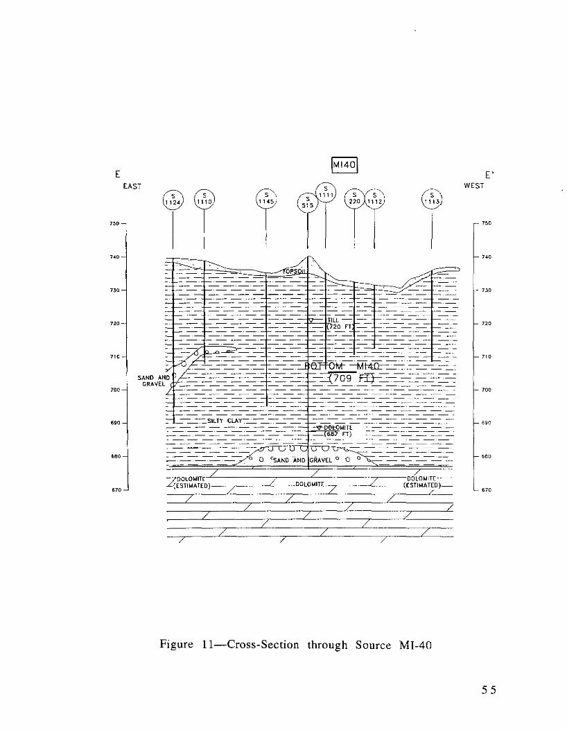
(3) The leached concentration is moved instantaneously to the edge of the "99% volume." This gives an initial concentration 6 feet (l.84 meters) below the bottom of the enclosure floor. Saturated conditions are assumed to occur below all sources in the glacial till. This is supported by boring data and water levels at each of the sources (see Figures 7 through 12). They show that the water table for all sources in the glacial till is above the source elevations, except for source N where it is 2 feet below the source elevation. The source N calculation uses a distance to the aquifer of 17 .7 meters. Reducing this distance by 2 feet to account for shorter travel in the saturated zone makes a small change in R(Till).
( 4) Since the leached concentration is now outside the "99% volume" region, it can be treated as a source of constant concentration, where production no longer takes place. This makes a clean break between production and decay. From this point on, one can begin with a constant concentration and migrate it through the local geology, taking into account its radioactive decay.
5. 2 The 99% Solution
Of these four independent parts, Part 1, the methods and numerics of taking 99% of the star density in the r and z dimensions, is discussed in Sections 5.3 and 5.4. Part 2, the 99% value of the leaching curve is explained in Section 5 .5. The reasons behind the assumption of Part 3, that the leached concentration is moved instantaneously away from the enclosure where unsaturated flow is possible into the saturated region, has been discussed in Section 2 of this report. Woodward-Clyde Consultants have done the migration calculations for Part 4, and their results are discussed in Section 7.
5. 3 Average Star Density
When high energy particles strike an object, there is a shower that builds up and then diminishes. The build up will generally occur within the shielding of the protected region. Figure 2 shows contours of equal star density S for a typical cylindrical beam dump
20
obtained in a CASIM calculation. Beyond shower maximum in the unprotected region, the fall off in the two dimensions varies as2 8
Exp(-2.S*r(meter)) and Exp(-1.0*z(meter))
Let rO and zO be the values at which the star density m each dimension has fallen to 1 % of its maximum value.
0 OlS - S * e-2.sro. ' max- max ' rO = 1.84 meters
Ools -S * -zO, • max - max e ' zO = 4. 6 meters
These limiting values define what we call the "99% volume" and it contains roughly 93% of the total radioactivity.
The average star density is given by
s = smax
rro rzo J
0Exp(-2.5r)rdr J
0Exp(-z)dz
rro rzo Jor dr J
0dz
where the first fraction is the average over r, and the second is the average over z. Smax is the maximum star density within the "99%
volume" and is obtained from CASIM. It is reasonable to use an average over a distance that is of the order of a few meters because the initial distribution is dispersed as water migrates through the till to the dolomite. 2 9
Putting in the above limits and doing the integrals gives,
S = Smax(0.089)(0.215) = (0.019)Smax
28 A. Van Ginneken and M. Awschalom, High Energy Particle Interactions in Large Targets, Vol. I. See pages 88-94 which shows the radial and longitudinal star density distributions for a concrete cylinder. 29 The dispersivity along the flow direction ranges from 0.9 meters for source MI-40 to 1.8 meters for source N (See Woodward-Clyde report, Tables 5-10). When one "looks back" at the source from the till/dolomite interface, points that originate closer together than the dispersivity cannot be distinguished from one another.
2 1
In the soil outside the "99% volume", the production of radionuclides is essentially zero. This cut off makes a clean break m which to "hand off" an initial concentration to Woodward-Clyde Consultants, because the edge is far enough away from the activation zone that it can be treated as a constant source. Projecting the "99% volume" in each dimension onto the r-z plane gives an activation area of approximately 3.7 meters by 4.6 meters. An area (called the "patch") is needed as input to the Woodward-Clyde calculations (see Section 7.3).
5. 4 Activation
Consider soil which gets activated by Np protons/year. If
water moves through the soil after many years of irradiation, then the activity in the water can be much higher than that for a single year. Observations by S. Baker at the DO Abort indicated that over a ten year period, "no percolation of rainwater in situ had removed the radioactivity from the soil". 30 Similar observations at the Proton Area led to the same conclusion. 31 It is therefore prudent not to take the activation at the end of one year, but to let it build up to it's saturation value, where the number of radionuclides being produced per unit time equals the number being lost due to decay per unit time.
The specific volume activity for isotope i is given by the production rate per unit time (qi) where
N *S* K. q.(pCi I cm3 -yr)= P
1
' r;*(l.17E6)
30s. Baker, "Fermilab Soil Activation Experience", Proceeding of the Fifth DOE Environmental Protection Information Meeting(Albuquerque. N. M.), Vol. 2, (1984), 673-683. 31 S. Baker, "Soil Activation Measurements at Fermi lab", Proceedings of the Third Environmental Protection Conference(Chicago. IL) U. S. Energy Research and Development Administration Publication ERDA-92, Vol. I, (1975), 337 and 345.
22
NP =the number of protons per year
S = the number of stars per cubic centimeter per proton
in the unprotected region
K; = the probability per star that an atom of nuclide i will be produced
'T, = the mean lifetime of nuclide i (yr)
l. l 7E6 = converts disintegrations per second into picoCuries (0. 037)
and years into seconds (3.15E7)
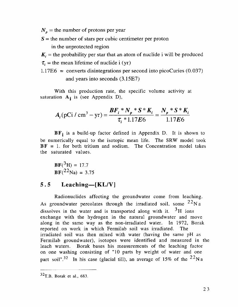
With this production rate, the specific volume activity at saturation Ai is (see Appendix D),
BF. *N *S* K. ~(pCi/cm3 -yr)= ' P '
r; *1.17E6
N *S* K. - p l
1.17£6
BF i is a build-up factor defined m Appendix D. It is shown to
be numerically equal to the isotopic mean life. The SRW model took BF = 1. for both tritium and sodium. The Concentration model takes the saturated values.
BF(3H) = 17.7
BF(22Na) = 3.75
5. 5 Leaching-[KL/V]
Radionuclides affecting the groundwater come from leaching.
As groundwater percolates through the irradiated soil, some 22 N a
dissolves in the water and is transported along with it. 3H ions exchange with the hydrogen in the natural groundwater and move along in the same way as the non-irradiated water. In 1972, Barak reported on work in which Fermilab soil was irradiated. The irradiated soil was then mixed with water (having the same pH as Fermilab groundwater), isotopes were identified and measured in the leach waters. Barak bases his measurements of the leaching factor on one washing consisting of "10 parts by weight of water and one
part soil". 32 In his case (glacial till), an average of 15% of the 22 N a
32 T.B. Barak et al., 683.
23
was leached out, and 100% of the 3H was leached (total tritium produced was not separated from leached tritium).
The amount of radioactivity leached out of a material (clay, sand, till, rock) is a function of (a) the amount of water that has moved through the material, and (b) the grain size of the material. Not all of the activity produced is picked up and transported by groundwater. In particular, measurements made on Fermilab soils
indicated typical percentages for 22Na of 1 % for rock,33 7% for sand
and gravel,34 and 15% for glacial till35•36 . One can think of these percentages as asymptotic values. What is of interest is the shape of the curve. As more water is added, more activity is leached. The
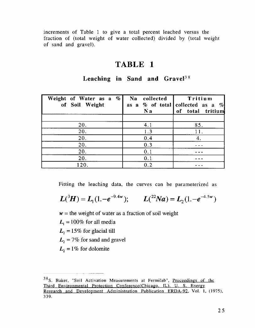
curve shapes for 3H and 22 Na are illustrated in Figure 4 (graphical representation of Table 1). The measurements of Table 1 come from introducing a large amount of water at the top of a column of sand and gravel and sequentially collecting a fixed amount at the bottom after percolation. Recently reported results37 from SSC rock confirm that the shape for rock is essentially the same as for sand and gravel. The same shape for the leaching curve is assumed for glacial till.
In order to put both the 3H and the 22 Na on the same plot, the y-axis of Figure 4 represents the percent leached divided by the asymptotic value (amount leached no matter how much water is added) for each nuclide. The rows in Table 1 are incremental measurements. For example, 4.1 % of the sodium and 85% of the tritium are leached out in the first sample of water collected which weighed 20% of the weight of the column of sand and gravel. The next sample collected (also 20% by weight) leached out an additional 1.3% of sodium and 11 % of tritium, etc. Figure 4 adds together the
33 s. Baker, private communication. In the mid-1980s, studies were done to determine the feasibility of siting the Superconducting Super Collider (SSC) in
Illinois. Fermilab would be used as the injector for this new and larger accelerator which was to be located below the surface in dolomite. Among the studies, S. Baker took a macroscopic sample of dolomite (about 2 inches by 2 inches), mixed it with one part water by weight and measured that the amount
of 22Na leached out of the dolomite was I%. 34s. Baker, "Soil Activation Measurements at Fermilab", Proceedin&s of the Third Environmental Protection Conference(Chicago. IL). U. S. Energy Research and Development Administration Publication ERDA-92, Vol. I, (1975), 337-339. 35 T.B. Borak et al., 686. 36P. J. Gollon, 6-9. 37 S. I. Baker, J. S. Bull, and D. Goss, "Leaching of Ellis County(Texas) Rocks", Health Physics 64, Supplement 1, (1993), page S89.
24
increments of Table 1 to give a total percent leached versus the fraction of (total weight of water collected) divided by (total weight of sand and gravel).
TABLE 1
Leaching in Sand and Gravel3 8
Weight of Water as a % Na collected Tritium of Soil Weight as a % of total collected as a %
Fitting the leaching data, the curves can be parameterized as
L(3 H) = LI (l.-e-9.4w );
w = the weight of water as a fraction of soil weight
L1 =100% for all media
L2 = 15% for glacial till
L2 = 7% for sand and gravel
L2 = 1 % for dolomite
38 s. Baker, "Soil Activation Measurements at Fermilab", Proceedings of the Third Environmental Protection Conference(Chicago. IL\. U. S. Energy Research and Development Administration Publication ERDA-92, Vol. I, (1975), 339.
25
Fraction Leached
1.1
0.9
0.8
0.7
0.6
0.5
0.4
0.3
0.2
0.1
0 0.2
Relative Amount of H or Na Leached vs. Amount of Water
Sodium (times 15.4)
Tritium
0.4 0.6 0.8
Weight of Water (as a fraction of soil weight)
1.2
Figure 4-Leaching curves for sand and gravel.
1.4
The leaching curves show that the more water that migrates through activated soil, the more radioactivity is leached out. However, saturation is achieved very quickly. By taking the 99%
26
point on the curves, one obtains w (weight of water)/(weight of soil) for each of the nuclides,
.99L1 = £i(1.-e-94w'); wl = 0.5 for tritium
.99L2
= L2(1.-e--i.swz); w2=1.0 for sodium
1.e., when an amount of water (by weight) equal to half the weight of soil is passed through it, 99% of all the tritium that can be leached out comes out. Similarly, 99% of all the sodium that it is possible to extract by the leaching process comes out when water in an equal amount (by weight) to that of soil migrates through it.
One can then transform the activity in the soil into a concentration in water by dividing the total activity in soil (Ai times
Vs) by the volume of water V w it takes to leach out 99% of its
asymptotic value. Combining the average star density, the build-up of
radioactivity to its saturation point in the soil, and the leaching curves, one can calculate an initial concentration c0 per year in
pCi/ml,
co( pCi ) = ~(pCi I cm3
- yr)* V,(cm3
) * L, ml - yr Vw(ml)
( Pei ) N * S * V * K. * L.
C - p s ' ' 0 -
ml-yr l.17E6 * Vw
Then changing the volumes into weights and densities, and
usmg the density of water as 1 gm/cm3 , and S = 0.019*Smax'
Vw = (Ww )(.&.) = p,(ww) = p, *w, V, Pw W, W,
27
NP = the number of protons per year
smax = the maximum stars per cubic centimeter per proton in the soil
K; = the probability per star that an atom of nuclide i will be produced
L; = the leaching fraction for nuclide i
p, = the density of soil(gm I cm3)
W; = the weight of water divided by the weight of soil
that corresponds to 99% leaching
1.17 E6 = converts disintegrations per second into picoCuries(O. 037)
and years into seconds(3.15E7)
5. 6 Propagation
Beginning with an average initial concentration, c0 , one obtains
the final concentration, Cr at a distance d away from a source by
multiplying by a factor (Rd) which comes from the consultant's
calculation of groundwater migration. Rd is made up of three terms
(a) a vertical migration in the glacial till from the elevation of the initial concentration to the top of the dolomite aquifer, (b) mixing with non-radioactive water at the glacial till/dolomite interface, and (c) horizontal transport in the dolomite to the nearest well or Site boundary:
These reduction factors were calculated by Woodward-Clyde Consultants and are given in Section 7. The final concentration 1s then,
At a distant point, any flow that goes into the drinking water from another part of the geometry where values are less than Sm ax
will have a smaller concentration since Smax was chosen at the
longitudinal position where the star density is maximum. Various
28
concentrations reaching the same well from different locations merely serve to dilute. That is, the average of the summed concentrations will always be less than c0 ,
where the subscript refers to different sources reaching the same final location.
This summing feature of the Concentration Model is in contrast to the SRW Model, where it is unclear if one has to sum over targets that are physically "close". For example, in the SRW Model, do the nuclides from both MP and ME (or PC and PE) add together and then get put into 40 gallons of water, or does each experimental target stand alone? How far apart do adjacent target areas have to be for them to be considered independent?
The Concentration Model answers the questions definitively. Targets (sources) are independent if they are separated by the "projected plane" of the "99% volume"-on the order of 5 meters. Secondly, by using the above equations for summing concentrations, the new model makes it clear that the combined concentration that results from the mixing from several points within the "99% volume" is less than or equal to the place having the highest concentration. Thus, by taking Smax we are being conservative. Of course, , summing has to be done over radionuclides at each final location, but not over geometry (space), nor over independent sources.
Model simulations were done for seven loss points. They are representative of Fermilab in terms of both plan view and elevation. The seven are: APO(Pbar Target), N(Neutrino), P(Proton), CO(Abort), AO(Extraction/Injection), MI-40(Main Injector Abort), and NUMl(Neutrinos at the Main Injector). The seven loss points and their elevations (at the position of the initial concentration) are given in Table 2 in addition to the coordinates of the 10 wells on site used for drinking water.
29
TABLE 2
The Seven Sources and Ten Drinking Water Wells
Location X(ft) Y(ft) Elevation(ft)
APO 100600 97950 718 N 100000 103500 737 p 100500 105900 722 AO 100000 100000 718 co 105207 102567 715 MI-40 101675 94420 709 NUMI 99100 98400 570
X and Y refer to the DUSAF coordinate system. Elevation is referenced from mean sea level. For the sources, the elevation is the position where the initial concentration is calculated. For the wells, the elevation is at the bottom of the well in the dolomite.
30
6 Protected and Unprotected Soil Regions
Soil activation occurs mostly near primary beam targeting and dump areas. The unprotected region is defined as that area of activated soil where radionuclides have the potential for reaching the aquifer due to leaching by groundwater percolating through it. Protected soil, on the other hand, either has no water percolating through it or else all of the water is collected. At Fermilab, particularly at the older targeting stations, dumps were designed to be surrounded by sand and gravel outside of the enclosure with an impermeable membrane, or "bathtub", under the sand and gravel to contain the radionuclides. Underdrains in the sand and gravel directly above the membrane were employed to collect any leached radioactivity and keep it from reaching the aquifer below. Newer targeting stations were built without a "bathtub", but still have sand and gravel, along with underdrains directly below the concrete floor. In some cases, these underdrains were used to define a protected region.
Underdrains can be quite effective when they are at the bottom of a very permeable medium such as sand and gravel, or when inside a bathtub, provided the media are saturated. In recent years, however, design strategies have generally employed massive concrete and steel shielding within enclosures to directly minimize the activation of the soil outside, rather than rely on water collection techniques. In addition, when unsaturated conditions exist near an enclosure, water may not travel through sand and gravel to the underdrains, but may travel around them as apparently occurred at Sheffield. See Section 2.2 where in unsaturated conditions, it is possible to have a higher flow through silty clay than through sand. It is not known definitively that the regions between the enclosure floor and any existing underdrains represent saturated conditions.3 9
The process of water collection from soil regions outside the concrete of an enclosure cannot be assured to be 100% efficient. It is heavily dependent on the location of the collection system, the soil type, and whether conditions are saturated or unsaturated. In fact,
3 9Fermilab's large and diversified monitoring program (collection of water samples from nearby wells and monitoring holes, and soil samples from dump and targeting regions outside of bathtubs) show no evidence for concentrations of radionuclides that exceed DOE or EPA guidelines for drinking water supplies.
3 1
the conditions may show seasonal vanat10ns between unsaturated and saturated, which make it a very complex problem. Furthermore, the integrity of "impermeable" barriers cannot be guaranteed. They are only as good as the seams that were "field installed". Stress and tension coming from differential settlement of the earth overburden could cause tears in the seams or the liner itself. Depending on the depth underground, damage could also come from roots or animal burrowing. Because of these uncertainties, we believe all soil outside the concrete of the enclosure should be considered to be unprotected, and all our results use this definition-drawing the line between protected and unprotected at the concrete/soil interface.
As evidenced in the dump example of Case 2 in Appendix E, an underdrain just below the building (necessary for structural considerations) may lead to the surface water limits controlling the thickness of the shielding in the dump rather than the drinking water limits in the aquifer. This of course assumes that water collected by the sumps is released at the surface immediately. If holding tanks or on-site storage are used, then the surface limits as discussed in Section 7.7 may not be an issue. In the design of a new facility, the designers might naturally be motivated by such considerations to move the underdrains lower. With the underdrains in a lower position, a strong temptation would exist to argue that the region between the bottom of the building and the location of the underdrains at the lower depth is well drained by the underdrains and is therefore protected. The discussion in the preceding paragraph points out some of the pitfalls of making such an argument.
32
7 Discussion of the WoodwardClyde Results
7 .1 Loss Points and Drinking Water Wells
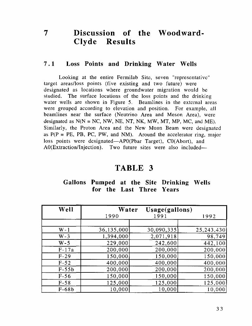
Looking at the entire Fermilab Site, seven "representative" target areas/loss points (five existing and two future) were designated as locations where groundwater migration would be studied. The surface locations of the loss points and the drinking water wells are shown in Figure 5. Beamlines in the external areas were grouped according to elevation and position. For example, all beamlines near the surface (Neutrino Area and Meson Area), were designated as N(N =NC, NW, NE, NT, NK, MW, MT, MP, MC, and ME). Similarly, the Proton Area and the New Muon Beam were designated as P(P = PE, PB, PC, PW, and NM). Around the accelerator ring, major loss points were designated-APO(Pbar Target), CO(Abort), and AO(Extraction/Injection). Two future sites were also included-
TABLE 3
Gallons Pumped at the Site Drinking Wells for the Last Three Years
MI-40(Main Injector Abort), and NUMI(Neutrinos at the Main Injector). These last two are particularly important, because MI-40 is the nearest to the Site boundary, and NOMI is deep underground, completely in the dolomite.
At the present time, there are ten wells on Site used for drinking water. Three wells, W-1, W-3, and W-5 are noncommunity, non-transient wells, meaning they serve the same group of non-residents at least 6 months of the year. The remammg ones (at former farm sites) are semi-private wells. Table 3 lists the water usage of each of the wells for the past three years. Measurements on W-1, W-3, and W-5 come from water meters; results for the other wells are estimates.
7. 2 Mathematical Models
Woodward-Clyde Consultants (WCC) used several analytical mathematical models to calculate how the concentration of radionuclides change as they migrate toward the aquifer. wee used the computer program called PATCH 3D, originally developed at the Center for Groundwater Research, University of Waterloo, Waterloo, Ontario to calculate R(Till) and R(Dolomite). They used the Depth of Penetration Model to calculate R(Mix).40
Calculations were done for ( 1) the vertical migration in glacial till to the top of the Silurian Aquifer in the dolomite, (2) mixing with non-radioactive water at the glacial till/dolomite interface, and (3) horizontal transport in the dolomite to the nearest well or Site boundary. Conceptually, these were separated into Model 1, Model 2, and Model 3 respectively. A schematic of the three Models is shown in Figure 6. Woodward-Clyde used the same analytic program (PATCH 3D) for Model 1 and Model 3. Model 1 and Model 3 transport in different physical directions, but the same program can be used by making a change of coordinates. The flow direction 1s defined as perpendicular to a "patch" containing the initial concentration.
Taking into account radioactive decay and dispersion, Model 1 migrates the initial "patch" downward to the dolomite. Model 2
40E. A. Sudicky et. al., PATCH 3D-Three-Dimensional Analytic Solution for Transport in a Finite Thickness Aquifer with First-Type Rectangular Patch (Waterloo, Ontario Canada: University of Waterloo, 1988). M. A. Sulhotra et. al., MULTIMEDIA-Multimedia Exposure Assessment Model for Evaluating the Land Disposal of Wastes Model Theory. EPA Contract#68-0l-3513 and #68-03-6304, (Chicago, Illinois: Woodward-Clyde Consultants, 1990).
34
calculates the vertical depth of penetration (H) into the upper portion of the dolomite. H and the till/dolomite properties are used to calculate the change in concentration which occurs as the vertically flowing plume from the glacial till mixes with the horizontally flowing groundwater in the dolomite. The mixing process is assumed to happen relatively fast, so no account is taken for radioactive decay in Model 2. Model 3 takes a "patch" size that was generated by Model 2, and transports it horizontally in the dolomite.
7. 3 Initial Conditions
Model 1 begins with a "patch", 3.7 meters by 3.7 meters, having an initial concentration c0 = 1., uniform in space and constant in time
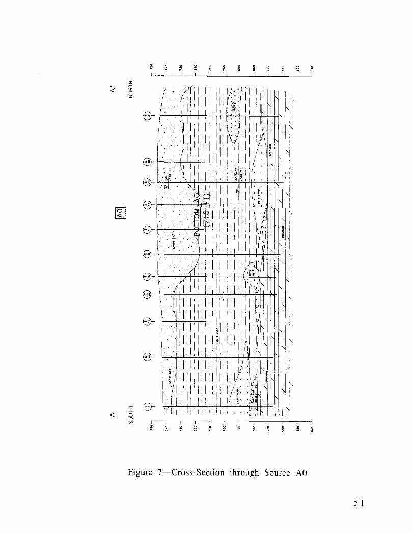
(see Figure 6). The projected area of activation at each source is 3.7 meters by 4.6 meters (see Section 5.5). However, so as to not bias the direction in any way at the seven sources, we gave a symmetrical "projected size" of 3.7 meters by 3.7 meters to Woodward-Clyde as input. The starting elevation is the elevation of the enclosure floor, minus the concrete thickness of the floor, minus 1.84 meters. (The maximum value of the star density will be at the edge of the concrete, and 1.84 meters farther out will encompass the "99% volume"). This patch is migrated over a distance to the glacial till/dolomite interface.41 Cross sections42 for the seven loss points are shown in Figures 7 through 13. In those cases where sand was present near the top of the dolomite, the distance to the interface was reduced to exclude the sand thickness. Such sand layers at the top of the dolomite can be seen for loss points APO, AO, CO, and MI-40. The vertically adjusted distances, along with the distance to the property boundary for each of the seven loss points are given in Table 4. All the sources except NUMI are located in the glacial till; NUMI is deep underground in the dolomite.
41 Woodward-Clyde calculates the reduction from the initial concentration at fixed locations after 50 years of migration. The average distance the "patch" travels may be greater or less than the distance to locations (like the till/dolomite boundary, the nearest well, or the site boundary) depending on the value of the seepage velocity. For example the distance travelled after 50 years for the representative velocity is 1 meter; for the high velocity, it is 20 meters. 42woodward-Clyde Consultants, Summary of Radionuclide Transport Madelin& for Ground Water at the Fermi National Accelerator Laboratory. Batavia. Illinois, Project Number 92C3073, August 1993, Figures 7-13.
35
TABLE 4
Vertical and Horizontal Distances from Each Source
Location Adjusted Distance to Distance to Distance to Boundary Boundary
Aquifer Along Gradien• (Shortest)
APO 10.7 m 1830 m 1160 m N 17.7 m 3050 m 1950 m p 11.6 m 3350 m 1680 m
AO 11.6 m 2380 m 1490 m co 15.2 m 1680 m 1680 m
MI-40 8.5 m 380 m 210 m NUMI -- - 2040 m 980 m
At the glacial till/dolomite interface, the 3.7 meter by 3.7 meter "patch" increases to a "patch" of size Lb by Lb as shown in
Figure 6.43 Model 2 uses Lb as an initial condition, together with the
aquifer properties of the glacial till and the dolomite, to calculate H. H is the depth of penetration of the plume into the dolomite layer. Model 2 and Model 3 use the same assumptions about the initial concentration. Model 3 is similar to Model 1, but the initial "patch" size is taken to have a size H by Lb.
7. 4 Input Data
Woodward-Clyde Consultants (WCC) was provided with approximately 250 borehole logs. In addition they were given water level readings from about 40 monitoring wells. Water levels were taken almost every year since the beginning of Fermilab in 1968 until 1987, when the Batavia office of the Illinois Water Survey was closed. Measurements were again taken in 1992, and these formed the basis of Woodward-Clyde's determination of the gradients. The
43 As explained in footnote 41. it is necessary to utilize the high value of the seepage velocity (0.4 m/yr) in order to determine Lb. At the representative
velocity, the "patch" doesn't travel far enough to reach the till/dolomite interface.
36
names, pos1t1ons, depth/water level for the monitoring wells and boreholes can be found in TM-1850.44
This information, plus several reports from SIS (Soil Testing Service), the Illinois State Water Survey, and the Illinois State Geological Survey enabled Woodward-Clyde to determine Site specific ranges for hydraulic conductivity, gradient, and effective porosity in both the glacial till and the dolomite. Data (TM-1850) from pump tests conducted in 1969 and 1970 on W-1 and W-3 were also used.
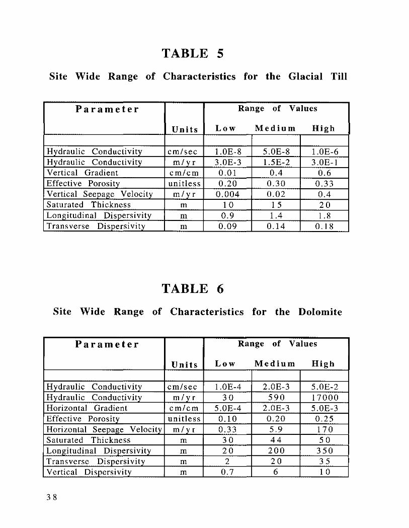
In Chapter 5 of their report, WCC discusses how the range of values for each of the input parameters was obtained from the numerous available data . The WCC numbers indicating the site wide ranges are duplicated below in Tables 5 and 6. For the medium and high values of the hydraulic conductivity in the glacial till (Table 5), WCC used previous work done on site by Soil Testing Services (STS).45
44A. A. Wehmann, A. J. Malensek, A. J. Elwyn, K. J. Moss, and P. M. Kesich, "Data Collection for Groundwater Study", Fermi National Accelerator Laboratory, Batavia, IL., Internal Report TM-1850, (1993). 45srs Report, "Additional Ground Water Flow Study, Anti-Proton Target Area, Fermi National Accelerator Laboratory, near Batavia, Illinois", August 31, 1978. This report states that the vertical velocity is between 0.013 and 0.021 m/year. The report was based on laboratory permeability tests of representative soil samples taken from two APO borings and a finite element flow net analysis utilizing 200 node points. To translate their measurements from the laboratory permeability tests to in situ results, SIS multiplied by a factor of five to obtain a vertical velocity range between 0.07 m/yr and 0.11 m/yr. SIS, "Report of Field Percolation Test Results", Memorandum #21, February 18, 1969. This report gives 3.0E-6 cm/sec as the high value for the hydraulic conductivity in "tough to hard" silty clay. Based on conversations with Ken Kastman of WCC (formerly with SIS and having extensive experience on Fermilab projects), the Woodward-Clyde consultants chose to use a slightly lower value (l.OE-6 cm/sec). The SIS percolation test results came from shallower soils which would have a higher hydraulic conductivity (because of root holes and crack) than deeper soils.
37
TABLE 5
Site Wide Range of Characteristics for the Glacial Till
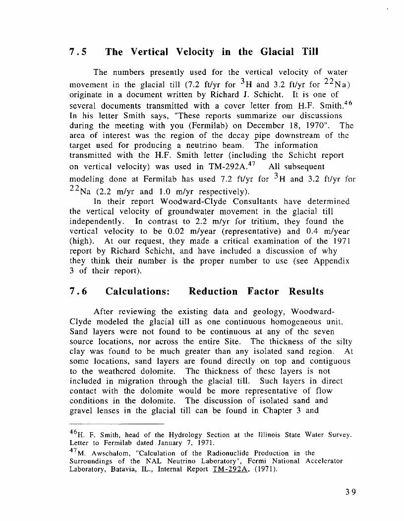
The numbers presently used for the vertical velocity of water
movement in the glacial till (7.2 ft/yr for 3H and 3.2 ft/yr for 22 Na) originate in a document written by Richard J. Schicht. It is one of several documents transmitted with a cover letter from H.F. Smith.46
In his letter Smith says, "These reports summarize our discussions during the meeting with you (Fermilab) on December 18, 1970''. The area of interest was the region of the decay pipe downstream of the target used for producing a neutrino beam. The information transmitted with the H.F. Smith letter (including the Schicht report on vertical velocity) was used in TM-292A.47 All subsequent
modeling done at Fermilab has used 7.2 ft/yr for 3H and 3.2 ft/yr for 2 2Na (2.2 m/yr and 1.0 m/yr respectively).
In their report Woodward-Clyde Consultants have determined the vertical velocity of groundwater movement in the glacial till independently. In contrast to 2.2 m/yr for tritium, they found the vertical velocity to be 0.02 m/year (representative) and 0.4 m/year (high). At our request, they made a critical examination of the 1971 report by Richard Schicht, and have included a discussion of why they think their number is the proper number to use (see Appendix 3 of their report).
7.6 Calculations: Reduction Factor Results
After reviewing the existing data and geology, WoodwardClyde modeled the glacial till as one continuous homogeneous unit. Sand layers were not found to be continuous at any of the seven source locations, nor across the entire Site. The thickness of the silty clay was found to be much greater than any isolated sand region. At some locations, sand layers are found directly on top and contiguous to the weathered dolomite. The thickness of these layers is not included in migration through the glacial till. Such layers in direct contact with the dolomite would be more representative of flow conditions in the dolomite. The discussion of isolated sand and gravel lenses in the glacial till can be found in Chapter 3 and
46 H. F. Smith, head of the Hydrology Section at the Illinois State Water Survey. Letter to Fermilab dated January 7, 1971. 47 M. Awschalom, "Calculation of the Radionuclide Production in the Surroundings of the NAL Neutrino Laboratory", Fermi National Accelerator Laboratory, Batavia, IL., Internal Report TM-292A, (1971).
39
Appendix 1 of the Woodward-Clyde report. In Appendix 1, they show that water flowing through isolated sand that is surrounded by clay is dominated by the hydraulic conductivity of the clay.
Some conservative assumptions that Woodward-Clyde uses are: (1) Flow in the glacial till is only in the vertical direction. (2) Flow in the dolomite is only in the horizontal direction. (3) Because the gradient in the dolomite is very small, its exact direction is uncertain, therefore the distance used in Model 3 is the shortest geometrical distance to the property boundary, not the distance along the flow line. They also made some calculations using the distance along the flow lines, but Table 8 contains the results for the shortest distance. ( 4) The reduction factors calculated by Model 2 assume that 100% of the vertical flux penetrating the glacial till/dolomite interface, is transferred into a horizontal flux.
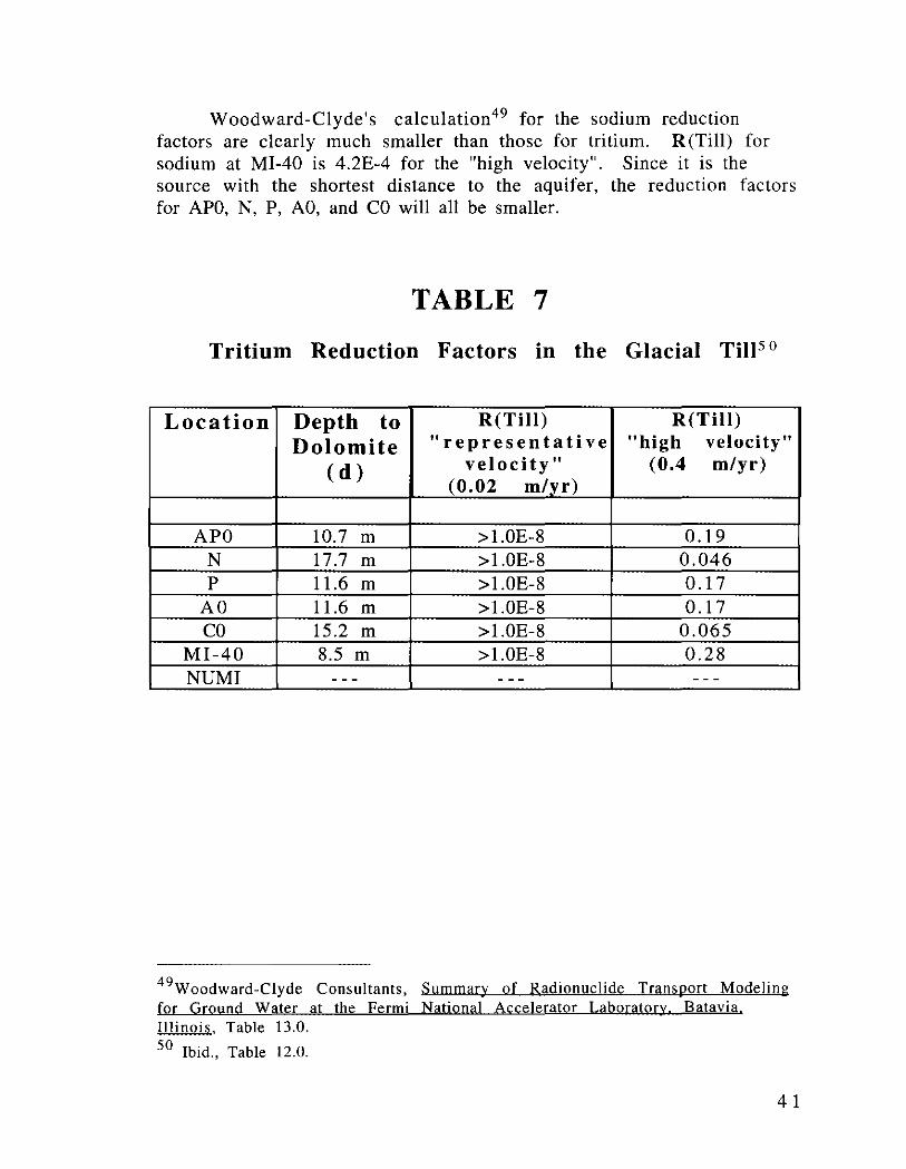
The reduction factors, R(Till), R(Mix), and R(Dolomite), as calculated by Woodward-Clyde are given in Tables 7 and 8. For R(Till) and R(Dolomite) the reduction factors are calculated after an initial concentration travels the appropriate distance from the source (the "patch"), where the source has been "on" for 50 years. Table 7 presents the results for the glacial till. A series of values are given for the "representative" velocity (0.02 m/yr), and another for the "high" velocity (0.4 m/yr). The "representative" velocity determined by Woodward-Clyde is the value that best represents the actual conditions at the Fermilab site (based on their experience and analysis of the data).
The tritium reduction factors in the glacial till given by Woodward-Clyde are plotted as a function of vertical distance from the source in Figure 14.48 Values of C!Co at the till/dolomite
interface (endpoint distance for each source) are shown in Figure 15. The line and its corresponding formula, l.7*Exp[-0.21 *d(meters)], represent an exponential fit to the endpoints. The results plotted in Figures 14 and 15 includes both dispersion (which is different for each source) and decay; the fall-off is steeper than for decay alone, which is Exp[-0.14*d(meters)].
48 The curves on Figure 14 for the "representative" velocity (0.02 m/yr) fall off more rapidly than those for the "high" velocity (0.4 m/yr), due to the fact that the concentrations shown are those after 50 years of radionuclide production. In 50 years, a radionuclide that moves with the "representative" velocity travels a distance of only I meter. The concentrations at distances larger than I meter are due to seepage velocities that exceed the average value-due to dispersion. The probability of radionuclides traveling at values different from the average velocity decreases rapidly the further one is from the average.
40
Woodward-Clyde's calculation49 for the sodium reduction factors are clearly much smaller than those for tritium. R (Till) for sodium at MI-40 is 4.2E-4 for the "high velocity". Since it is the source with the shortest distance to the aquifer, the reduction factors for APO, N, P, AO, and CO will all be smaller.
TABLE 7
Tritium Reduction Factors in the Glacial Ti115 °
Location Depth to R(Till) R(Till)
Dolomite "representative "high velocity"
(d) velocity" (0.4 m/yr) (0.02 m/vr)
APO 10.7 m >l.OE-8 0.19 N 17.7 m >l.OE-8 0.046 p 11.6 m >l.OE-8 0.17
AO 11.6 m >l.OE-8 0.17 co 15.2 m >l.OE-8 0.065
MI-40 8.5 m >l.OE-8 0.28 NUMI - - - - - - - - -
49woodward-Clyde Consultants, Summary of Radionuclide Transport Modeling for Ground Water at the Fermi National Accelerator Laboratory, Batavia, Illinois, Table 13.0.
SO Ibid., Table 12.0.
4 1
TABLE 8
Tritium Reduction to the Nearest
Location Distance (d)
APO to W-1 370 m N to W-3 390 m P to F-52 510 m
AO to W-1 350 m CO to F-55b 220 m
Ml-40 to Bndry 210 m NUMI to W-1 240 m
Factors in Well/Site
R(Mix)
0.18 0.22 0.20 0.16 0.27 0.24 -- -
the Dolomite Boundary
R(Dolomite)
0.0067 0.0056 0.0021 0.0080 0.0271 0.0253 0.0030
Table 8 contains one column for the reduction factor at the till/dolomite interface (Model 2) and another for the reduction factor in the dolomite (Model 3). The values of R(Mix) for APO and MI-40 in Table 8 are taken directly from the Woodward-Clyde report. The others are not available in the wee report and have been calculated by us. The values of R(Dolomite) in Table 8 are either found directly in the wee report or can be interpolated from the tables of R(Dolomite) vs. distance that WCC has given for the source points.
To calculate R(Mix) we note that the WCC formula51 4-1 and 4-2 can be written as
H(meter) = ..j(2.)(20.)(d(meter) / 300.) 12.
+ Vh( meter I yr)
R(mix) = Vv * nv *Lb = (0.4)(0.3)(20.) = 12. Vh * nh * H (Vh)(0.2)H Vh * H
This expression for H results from noting that the exponential m 4-1 can be approximated by the expression Exp(-A) = 1 - A,
5 1 Ibid., Chapter 4 page 4-6. V v, nv, and Lb, respectively, are the seepage velocity, effective porosity, and the horizontal length of the plume in the glacial till. V h, "h, and H, respectively, are the seepage velocity, effective
porosity, and the vertical length of the plume in the dolomite.
42
since A is numerically small. In both equations above, the number 12 represents the same quantity.
Because of their proximity to a well, some sources can experience larger gradients as a result of pumping. Such is the case for APO, AO, and NUMI. Well W-1 induces a larger gradient than the natural gradient, therefore R(Mix) for AO is calculated with V h = 8.9
meters/yr and d = 350 meters. The pumping rates for the other wells are so low that the induced gradients are smaller than the natural gradient, so the N, P, and CO calculations use V h = 5.9
meters/yr and the distance d as given in Table 8. The values of R(Dolomite) presented in Table 8 for APO, MI-40,
and NUMI are taken directly from Appendix 5 of the WCC report. AO is interpolated from "APO Model 3 Induced Gradient to Well W-1" by taking the reduction at d = 350 meters. N, P, and CO can be approximated by taking the results from "APO Model 3 Natural Gradient to Closest Property Boundary" and substituting the appropriate distance between each loss point and the nearest well (d). Of the seven loss points, MI-40 is the only one where the distance to the Site boundary is shorter than the distance to the nearest well.
Woodward-Clyde made sodium calculations for MI-40 and NUMI. It found a sodium reduction factor of 4.2E-4 for MI-40 to the site boundary, and 3.0E-5 for NUMI to W-1 which is 240 meters away. The values for APO, and AO can be approximated from the "NUMI Model 3 Induced Gradient to Well W-1" by substituting the appropriate distances and N, P, and CO can similarly be approximated from "NUMI Model 3 Sodium." As before, the sodium reduction factors are much smaller than the corresponding tritium results.
7. 7 Regulations and the Annual limit
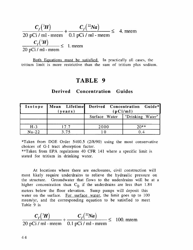
Limits for groundwater and surface water are found m chapter 3 of the Fermilab Radiological Control Manual. It contains a list (selectively reproduced in Table 9) of derived concentration guides for common accelerator produced radionuclides. The tritium and sodium limits come from two different regulations--DOE Order 5400.5 and EPA 40 CFR 141. For drinking water, the former specifies a limit of 4 mrem/yr, while the latter specifies 1 mrem/yr.
A person will receive an annual effective dose equivalent of 1
mrem if the drinking water contains either 20 pCi/ml of 3H, or 0.1
pCi/ml of 22 Na. Using these conversion coefficients for tritium and sodium, the annual limits can be expressed as
43
C1 (3H) C1 (22Na)
----~~---+ < 4. mrem 20 pCi I ml - mrem 0.1 pCi I ml - mrem
C1 (3H) ---~-~--< 20 pCi I ml - mrem -
1. mrem
Both Equations must be satisfied. In practically all cases, the tritium limit is more restrictive than the sum of tritium plus sodium.
TABLE 9
Derived Concentration Guides
Isotope Mean Lifetime Derived Concentration Guide* (years) (pCi/ml)
Surface Water "Drinking Water"
H-3 17. 7 2000 20** Na-22 3.75 1 0 0.4
*Taken from DOE Order 5400.5 (2/8/90) usmg the most conservative choices of G-1 tract absorption factor. **Taken from EPA regulations 40 CFR 141 where a specific limit is stated for tritium in drinking water.
At locations where there are enclosures, civil construction will most likely require underdrains to relieve the hydraulic pressure on the structure. Groundwater that flows to the underdrains will be at a higher concentration than c0 if the underdrains are less than 1.84
meters below the floor elevation. Sump pumps will deposit this water on the surface. For surface water, the limit goes up to 100 mrem/yr, and the corresponding equation to be satisfied to meet Table 9 is
c1 (3H) c1 (22Na)
---~~~--+ ::; 100. mrem 20 pCi I ml - mrem 0.1 pCi I ml - mrem
44
7. 8 Application of Results
According to the IEPA's classifications, all groundwaters are Class I unless demonstrated otherwise. Class I is the State of Illinois' designation for potable groundwater supplies currently being used as well as those having the potential to be developed. Furthermore, Class I applies only to groundwaters below a depth of 10 feet from the surface. The dolomite is clearly Class I, but the glacial till is not for at least two reasons: (1) Its hydraulic conductivity is much Jess than lE-4 cm/sec, and (2) the amount of water that can be pumped from it is far less than 150 gallons/day.
As mentioned in Section 5.6, Woodward-Clyde was asked to calculate reduction factors for the glacial till, the dolomite and the interface between them. The final concentration is,
Exactly where is the compliance point for meeting the groundwater quality standards? How should Cr be calculated? In
the glacial till the groundwater is clearly not Class I, so R(Till) as found in Table 7 can be used. It is unclear whether R(Mix) from Table 8 can be used. Although mixing is going on, it is natural mixing between two layers with different groundwater classifications. This is clearly separate from man-induced mixing where the amount of mixing can be arbitrary. Groundwater in the dolomite is Class I, so credit cannot be taken for dilution as it migrates from one location to another. 52 Therefore, one must take R(Dolomite) = 1.53
5 2 A point has been raised about the possibility of designating portions or all of the Fermilab site as a "groundwater management zone". However, such a classification, even if granted, would require the zone to be managed under corrective action and mitigation of the contaminant. Since the lab still wants to continue running experiments, no advantage is gained. 53 Jn addition, this avoids having to defend the dolomite as a porous medium. Although there is no evidence for fracture flow at the Fermilab Site, Section 2.4 gives two such examples at nearby locations.
45
For the six sources in the glacial till (APO, N, P, AO, CO, and MI-40) the final concentration is
c1 ( pCi J = C0 * R(Till) * R(Mix) ml-yr
For a source like NUMI which is entirely in the dolomite, it may be necessary to modify c0 (see Appendix E, Case 3).
An overall policy addressing these issues should be developed by the Environment, Safety, and Health Section with the approval of the Fermilab Directorate. This report presents the methodology and the resulting reduction factors in Tables 7 and 8. It will be the policy document which finally states whether R(Till) will be taken for the "representative" velocity, the "high" velocity, or somewhere inbetween. It will also give guidance on how and when to apply R(Mix) and R(Dolomite) for sources in the glacial till.
For illustrative purposes, we take R(Till) and R(Mix) from Tables 7 and 8, but take R(Dolomite) = 1. Several numerical examples are given in Section 7.9 and Appendix E. Obviously, they can be modified appropriately to comply with the Fermilab Policy Statement.
7. 9 Numerical Examples
The relevant equation to calculate the initial concentration 1s,
co( pCi ) = NP* [(0.019) * S(max)] *Ki* Li
ml-yr 1.17E6 * Ps *Wi
46
N, =the number of protons per year
Sm,, = maximum stars per cubic centimeter per proton in the unprotected soil
K; =the probability per star that an atom of the ith nuclide will be produced
L, = the leaching fraction for the ith nuclide
p, = the density of soil (gm I cm3)
w; = the weight of water divided by the weight of soil
that corresponds to 99% leaching
l.17E6 = converts disintegrations per second into picoCuries(O. 037)
and years into seconds(3. l 5E 7)
Depending on whether the source is in glacial till or dolomite, one chooses the corresponding numbers from Table 10 and substitutes them into the equation for Co. By obtaining Smax from
CASIM, one calculates the initial tritium and sodium concentrations. Often it is more convenient to calculate one isotope and use ratios to evaluate the other one. Using Table 10 one finds
c0(3H)tC0(22Na) = 50. for glacial till, and
c0(3H)/C0(22Na) = 300. for dolomite
Once values of c0 are obtained for 3H and 22Na, they are put
into the first two equations of Section 7. 7 to determine if they meet the groundwater limits. If the loss point (source) is in an enclosure, c 0 must be extrapolated to the elevation of the underdrains (Cu),
then substituted into the third equation of Section 7 .7 to determine if the surface water limit is met. This assumes water entering the sumps is immediately discharged as surface water.
To illustrate the principles used in the concentration model, detailed numerical calculations for three cases are given in Appendix E. They are (1) a buried pipe, (2) a 4 ft radius iron dump, and (3) a neutrino beam in dolomite.
47
TABLE 10
Parameter Values in Glacial Till and Dolomite
Parameter Glacial Till Dolomite
3H 22N a 3H 22N a
~ 0.075 0.02 0.03 0.02
L· I 1.00 0.15 1.00 0.01
Pi 2.25 2.25 2.67 2.67
W· I
0.5 1.0 0.5 1.0
Leaching measurements in Fermilab dolomite were made for sodium, but not for tritium. The tritium number of 0.03 is taken from S. Baker's tritium measurements on rock formations at the
SSC54.
54 S. I. Baker, private communication. The value of 0.03 includes the conservative case where the rock was in contact with water for one year. See also S. I. Baker, J. S. Bull, and D. Goss, "Leaching of Ellis County(Texas) Rocks", Health Physics 64, Supplement 1, (1993), page S89.
48
'
1001
W-3 •
F-68b •
e p ew-s2
eM140
• \.1-56
• V-5
/ /
/
·\.1-::B
W\.
•
Figure 5-Representative Loss points (sources) and Drinking Water Wells
Figure 15-Concentration Reduction in the glacial till as a function of Endpoint Distances to the till/dolomite interface for each Source. The seepage velocity is 0.4 meters/yr
59
8 Summary
The SRW Model has been used since Fermilab's inception to determine the quantity of radionuclides entering the aquifer. It 1s based on several simple conservative assumptions. With the increased attention given across the country to environmental investigations and the siting of landfills, more resources have been brought to bear on techniques for calculating the groundwater migration of contaminants. A new Concentration Model is proposed which takes advantage of such calculations. The essential features of the Model are to consider a loss point surrounded by steel, concrete, and soil. All soil beyond the concrete is considered "unprotected." The activity in the soil is obtained by taking the highest value of the star density within the unprotected region and averaging it over a volume that contains 93% of the produced radionuclides (this is called the "99% volume" because in this region, the star density has decreased to 1 % of its maximum value in both the r and z dimensions.
An amount of water sufficient to leach out 99% of the asymptotic value of the radioactivity is passed through the soil of the "99% volume" to give a corresponding concentration of activity m water. The leached concentration is moved instantaneously to the bottom edge of the "99% volume" and this defines the initial concentration c0 . Taking c0 as uniform in space and constant in
time, Woodward-Clyde Consultants calculated reduction factors for ( 1) the vertical migration through the glacial till-R(Till), (2) the till/dolomite interface-R(Mix), and (3) the horizontal migration through the dolomite-R(Dolomite). The results of their calculations are summarized in Tables 7 and 8.
For tritium, two values of R(Till) are given: one for a "representative" velocity, and another for a "high" velocity. The concentration reduction factors in the glacial till and the dolomite depend on hydraulic conductivity, the gradient, and the porosity of the medium. Of all the parameters, the largest uncertainty is the value of the hydraulic conductivity in the glacial till, which ranges from 5E-8 cm/sec (representative) to IE-6 cm/sec (high). Because it enters into an exponential, small variations can make large changes when the reduction factors are calculated. The reduction factors for sodium are much less than those calculated for tritium at each source.
60
R(Mix) and R(Dolomite) vary as a function of distance from the source to the nearest well or Site boundary. The results in Table 8 use the shortest distance, not the distance along the flow lines.
Woodward-Clyde Consultants recommend a field program to reduce the range of values. They suggest the installation of four depth specific piezometer clusters at each of the seven sources. The four wells would be screened in (1) the upper glacial till, (2) the lower glacial till, (3) the upper dolomite, and (4) the lower dolomite. In addition, they recommend the installation of three similar piezometric clusters far away from the sources near the north, west, and east boundaries of the Site. Slug tests and pump tests on these and all monitoring wells would establish narrower ranges for each of the input parameters. The committee believes this report presents calculations which are based upon a realistic range of parameters that are available now. Future calculations can be done to update Tables 7 and 8 after additional field work narrows the range of hydraulic conductivity.
The Concentration Model can be summarized briefly by the two equations,
( pCi J- NP* [(0.019) * Smax] *Ki* Li Co -----"-~~~~~~~~~~~~~~
Cr is then compared to the limits specified in the Fermilab
Radiological Control Manual.
Our report discusses each of the independent factors which make up these equations and we have illustrated their use by giving numerical examples for various conditions. Most of the terms in the equations use the extreme limits. The conservative features are:
• Take instantaneous movement of groundwater through the unsaturated zone.
• Begin the region of unprotected soil at the edge of the concrete.
• Within the unprotected region, take the point having the highest star density smax.
6 1
• Take radioactive build-up to saturation (which for tritium would take over 50 years of continuous running).
• Minimize all distances by taking only vertical flow in the glacial till, only horizontal flow in the dolomite, and the shortest distance to the nearest well/Site boundary.
If the Concentration Model is adopted, the Environment, Safety, and Health Section will propose a laboratory policy to the Fermilab Directorate for their approval. The policy should be specific enough so that final concentrations can be calculated and compared to the annual limits set forth in the Fermilab Radiological Control Manual. We believe the policy should address the following choices:
62
• Should radioactive build-up in the soil be taken to saturation, or some smaller number? Alternating one year of continuous running followed by one year off gives about a factor of two lower in the asymptotic value. Even for our highest source (APO), the amount of real operating time is far less than continuous.
• Is averaging over our definition of the "99% volume" appropriate for both the glacial till and the dolomite?
• Should the 99% point on the leaching curve be taken? If the first measured point on the curve is taken where the amount of water is 20% by weight, then the initial concentration increases about a factor of two.
In addition, the following items are identified and discussed further below and in the numerical examples of Appendix E:
• What value should be taken for R(Till), R(Mix), and R(Dolomite)?
• Where should the line be drawn between the protected and unprotected zones? Is this the same for existing facilities and new construction?
• Can water collected from the underdrains be kept in holding areas, or should underdrains be designed far enough away so any water collected will meet the surface water limit and can be disposed of immediately?
• For tritium, what leaching value should be taken for sources in the dolomite? (The KL value given in Table 10 is only an estimate).
R(Till) depends on the seepage velocity in the glacial till. Will it be taken for the representative velocity, the high velocity or somewhere in-between? If an intermediate velocity between 0.02 meter/yr and 0.4 meter/yr is chosen, for example something like 0.1 meter/yr (based on the highest value from the STS measurements and analysis at AP055 ), the computer program PATCH 3D can be run to obtain new reduction factors. These corresponding values would replace those now in Tables 7 (which would have only one column). We are in the process of purchasing the PATCH 3D software, so that should not present an obstacle to choosing a velocity different from those represented in Table 7. The Woodward-Clyde discussion (in Appendix 3 of their report) of the velocity used in the SRW Model may also be helpful in choosing a velocity.
Because R(Mix) is at the interface between the glacial till and the dolomite, it is a function of distance to the nearest well/site boundary and the properties of each media. Natural mixing is taking place as the vertically moving contaminated groundwater in the till is combining with the horizontally moving non-contaminated groundwater in the dolomite. For simplicity, it might make sense to take the same number for all sources, say R(Mix) = 0.27, which is the maximum in Table 8.
Because groundwater in the dolomite is Class I, we believe one must take R(Dolomite) = 1. Making this choice also avoids having to defend the dolomite as a porous medium. Although there is no evidence for fracture flow at the Fermilab Site, Section 2.4 gives two such examples at nearby locations.
In our sample calculations, we draw the line between protected and unprotected at the interface between the enclosure concrete and the soil. The integrity of "impermeable" barriers in the soil cannot be guaranteed, nor can underdrains in the soil be assured to be 100% efficient for water collection. It is important to point out, that when underdrains are installed for purposes of relieving the hydraulic pressure on a structure, their location can affect how much shielding goes into the protected region (See Case 2 in Appendix E). If the water collected from the underdrains and sumps goes first to a storage area, it has to meet the surface water limits only when water from the storage area is discharged to surface streams, swales, etc. If there is a procedure to assure these discharges are below the surface water limits when released, then the amount of shielding in the protected areas is governed only by the sub-surface drinking water
55 STS Report, "Additional Ground Water Flow Study, Anti-Proton Target Area. Fermi National Accelerator Laboratory, near Batavia, Illinois", August 31, 1978.
63
standards. This issue is complicated by the fact that there are underdrains in almost all of our existing enclosures. It might make sense in the policy to address underdrains for new construction separately from those in existing facilities.
Table 10 gives the numerical values used to calculate c0 . Most
of these have been measured at Fermilab. However, the leaching factor (KL) in dolomite for tritium has only been estimated. Furthermore, before constructing a source like NUMI it will be necessary to know the extent of the protected and unprotected regions. All numerical terms will have to be established to calculate Cr (see for example Case 3 in Appendix E). Borings at the NUMI
location have recently been completed, and samples should be irradiated to make a measurement of the tritium leaching factor.
For new construction it should be required that there be enough soil borings through the glacial till down to the dolomite to establish if and where the sand is. As should be clear from Figures 7 through 12, it is important to know the geologic cross-sections at each source. Appropriate judgments can be made to correct for the position and amount of sand. Finally, the reduction factor calculations use the existing ten drinking water wells which are all in the dolomite. The drilling of new wells or increased pumping from them affect groundwater migration primarily by changing the gradient. The trend over the past three years (See Table 3 ), indicates that less water is being pumped from the main wells W-1 and W-3, more from W-5, and the others are about the same. Certainly, no new drinking water wells should be installed near sources nor potential sources, without understanding how they would affect Tables 7 and 8.
64
9 Acknowledgments
Special recognition needs to be given to several individuals who helped us obtain the data which finally went to Woodward-Clyde Consultants. The locations of the numerous wells and the soil borings were obtained from the Site Alignment Group. The coordination and scheduling, as well as obtaining special equipment from outside the laboratory (global positioning system using satellite transmissions), was handled by Terry Sager and the late Tom Nurczyk. Diana Bonham consolidated the various pieces of information on the bore hole drillings and the wells, put them on single maps, and extracted the coordinates. They also provided us with DXF files which could then be easily given to Woodward-Clyde.
Throughout we have relied on the work and experience of Sam Baker. The fruits of his many years of firsthand involvement with monitoring and measuring radioactivity proved to be helpful in setting the priorities for our efforts. We benefited greatly from his files in the ES&H Section . His familiarity with Fermilab, his ongoing measurements at the SSC, and his expertise enabled us to confidently estimate parameters for which we had no local data.
Bob Sasman was invaluable to us because of his long experience with the Illinois State Water Survey. His advice and expertise helped us sort out much of the important from the unimportant, and saved us from going down many dead ends. He located the older water level data and then did the 1992 water level measurements at our site wells. He furnished us with pump test results that were done during the early days of Fermilab. In addition, he obtained many documents from the Illinois State Water Survey, the Illinois State Geological Survey, and several other agencies that greatly assisted us in doing our study.
There are several other individuals we'd like to thank. One of us (A.W.) attended a course entitled "Groundwater Flow Through Fractured Media" at the University of Wisconsin, Madison, in March, 1992. One of the instructors, Peter L. Monkmeyer, Professor and Chairman of the Department of Civil and Environmental Engineering at UW, was very helpful in private conversation and supplied us with a list of books that we found quite useful. We'd like to thank Norbert Golchert, head of the Environmental Protection Division at Argonne National Laboratory, for his hospitality during a 2/21/92 visit by one of us (A.W.). He supplied us with the latest USGS reports on studies of the Low-Level Radioactive-Waste Burial Site at the Palos Forest Preserve, southwest of Chicago.
65
1 0 Appendices
1 0. 1 Appendix A-Hydraulic Conductivity as a Function of Pressure
K
Figure 16-Characteristic curves for hydraulic conductivity (K), versus pressure (\jl) for (a) sand, (b) silty sand, and (c) silty clay
[After Freeze and Cherry, p. 43).
Figure 16 shows the relationship between hydraulic conductivity and pressure. Unsaturated flow takes place in the region where the pressure is negative and the curves for the various soil types cross one another. For example, the hydraulic conductivity of sand [Curve(a)] is smaller than silty clay [Curve(c)] at large negative pressures, but the opposite is true at small negative pressures. Large negative pressures represent dry soil conditions. As rain fall on dry soil, water moves preferentially around the sand and through the silty clay (because flow is in the direction of largest hydraulic conductivity). However, after the soil gets more wet, the pressure increases, the hydraulic conductivity for sand gets larger than for silty clay and water then flows preferentially through sand. It should be clear that seasonal and short term conditions as well as history determines unsaturated flow, and the constantly changing variables is what makes it so difficult to calculate and defend.
This is in sharp contrast to saturated flow which takes place in the region where the pressure is positive, and the hydraulic conductivities are constant for each soil type. No matter the value of
66
the pressure, sand always has a larger hydraulic conductivity than silty clay. When the hydraulic conductivity is constant, the differential equations are easier to solve, and the fact that the pressure is not the same everywhere, doesn't matter.
10.2 Appendix B-Travel Through the Unsaturated Zone and Capillary Fringe
Case 1-The Illinois State Water Survey correlated precipitation and shallow groundwater levels in 20 wells scattered across the state. Data was used for the years 1960-1984. Shallow groundwater indicates the level of the water table, so the time it takes to arrive at the water table is a measure of how long it takes to pass through the unsaturated zone and the capillary fringe. The analysis of the data showed that the characteristics of the soil (soil type) was the primary indicator that determined the time lag between precipitation falling on the surface and an increase in the water table level. 56 In the northern 2/3 of Illinois, a lag time less than one month gave the best fit to the data. A lag on the order of two months is found for southern Illinois. Of the twenty data points, the one closest to Fermilab is in DuPage county and is labeled data point #4. Summary Tables 4 and 5 in the article list its soil type as glacial till in a dolomite aquifer-essentially the same as Fermilab. The same Tables report a mean depth to water of 3.87 meters.
Case 2-Soil surveys have been done by the US Department of Agriculture for DuPage and Kane counties. The portions of the report relevant to Fermilab are map sheets 60 and 65 in DuPage County. For Kane County it is sheets 48, 53 and inset B and C of sheet 64. These maps show contours of soil types. They indicate that the preponderance of Fermilab is covered by 152(Drummer), 442(Mundelein), and 697(Wauconda) soils. Smaller amounts of 443B(Barrington), 698B(Grays) and 531B(Markham) are also present. Of the six types mentioned above, all except Markham list rates from 0.6 to 2 inches/hr. Markham has the same rate for the top 12 inches, but at depths from 12-60 inches the rate is 0.06 to 0.6 inches/hr.The
5 6stanley A. Changnon et al., "Relations Between Precipitation and Shallow Ground water in Illinois", Journal of Climate, I, (1988), 1248.
67
rate at which water moves through the soils is found in Table 14-
Physical and Chemical Properties of Soils.57 •5 8
Using an average of the rates and the same distance to the water table as before (3.87 meters), one gets a lag time of 5 days for the first five soil types and 19 days for the Markham. This is consistent with the Illinois State Water Survey data point#4, but has the advantage of actually being specific to the Fermilab Site. Multiyear (January 1989-December 1991) water level measurements59 at well 39d show a maximum depth of about 10 feet below the land surface, so the lag times are even smaller. The essential point is that water falling on an "open, level field" spends only a matter of days traveling through the unsaturated zone and the capillary fringe. We thus take no credit for any phenomena that may take place above the saturated zone, and will treat the initial concentration (Co) the
same as if it were transported instantaneously from the edge of the unprotected region to the saturated zone.
1 0. 3 Appendix C-Fracture Flow in Dolomite
Case 1-Darien, IL., (Southeast DuPage County) 2174
Analysis showed a public supply well, Brookhaven Manor Water Co. Well No. 5, was contaminated. It is 320 feet deep, finished in dolomite, and cased to 108 feet, with a capacity of about 400 gallons per minute. An "abandoned" well-scaling from the sketch in the 2/20174 memorandum on the incident by R. Sasman-is about 800 feet away and 300 feet deep. On 2/8174 Well No. 5 was pumped to see what effect it had on water levels in the "abandoned" well, in a private well between the "abandoned" well and Well No. 5, and Well No. 6 (also at Brookhaven Manor). The first round of pumping began at 10:15 AM, and terminated at 11:02 AM. Meantime, at 10:40 AM, 1500 gallons of
57 0. R. Mapes, Soil Survey of DuPage and part of Cook Counties. Illinois(also called Illinois Agriculture Experiment Station Soil Report No. 108), (Washington D. C., US Government Printing Office 1979), 204-209. 58 Tyrone M. Goddard, Soil Survey of Kane County. Illinois(also called Illinois Agriculture Experiment Station Soil Report No. I 09), (Washington D. C., US Government Printing Office 1979), 171-174. 59 A. A. Wehmann, A. J. Malensek, A. J. Elwyn, K. J. Moss, and P. M. Kesich, TM-1850, (1993).
68
liquid chlorine were injected into the "abandoned" well-a process that took until 12:30 p.m. Pumping was started again at Well No. 5, at 2:45 p.m. and after 18 minutes the pumping effluent took on a red hue indicating the effect of the chlorine compound interacting with iron compounds in the subsurface. At 25 minutes of pumping, a test indicated a chlorine concentration of more than 10 mg/liter. (A check with the DuPage County Health Department elicited the fact that the liquid chlorine utilized had 12% by weight of sodium hypochlorite.)
The memorandum says that there was no report of chlorine (i.e. red color) in any well other than well No. 5. Since the private well is between the abandoned well and Well No. 5, and is almost exactly on the line drawn between them, it might have been expected to show some evidence of the chlorine. R. Sasman interprets the lack of chlorine in the private well to indicate that the channel network between the abandoned well and Well No. 5 was not being intercepted by whatever fractures are being utilized by the private well part way between them.
Case 2-Palos Park, IL., (Southwest Cook County) 12177
The well used for the pump test was located at the Commons of Palos Park. It is 410 feet deep and finished in the Silurian Dolomite. Three other wells were used as observation wells-(1) US Post Office at Palos Park, 155 ft deep and 380 feet away, (2) Daly Company, unknown depth and 500 feet away, and (3) Lumber Company, unknown depth and 700 feet away.
The Commons well was pumped for 315 minutes at a rate of 284 gpm, after which the drawdown in Observation Well 1 was 4.7 feet, Observation Well 2 was 6.0 feet, and Observation Well 3 was 7 .6 feet. This is a clear example of fracture flow. If the medium between the wells was porous, then the observation wells would have shown decreasing drawdown as the distance from the pump increased.
69
10.4 Appendix D-Build-up to Saturation
Let qi be the rate of production per unit time. Then, the
activity Ai can be written as production minus decay.
A; dA. = q. dt--dt ~ l ~-
I
Solving for Ai and imposing the condition Ai(t=O) = 0, gives
Saturation is reached at times long compared to the isotopic mean life, so that
~(saturation)= qi ii
If decay is neglected, then the above equation for activity can be written as
dA; =qi dt Imposing the same initial condition as before, Ai (t=O) = 0, the
solution at time t is
A. =q.t I I
Defining the build-up factor BF as the ratio of the activity at saturation to that after one year (without decay) leads to,
BFi = (qi'ti)/[(qi)(lyr)] = 'ti/lyr
That is, the build-up factor is numerically equal to the mean life. Thus,
70
BF( 3 H) = 17.7
BF( 22 Na) = 3.75
1 0. 5 Appendix E-Numerical Examples
Case 1-Long Buried Pipe
Case 1 is a 50 cm target (radius = 6 inches) followed by a long buried pipe having an outer diameter of 12 inches and a wall thickness of 3/8 inch (see Figure 17). Such a situation might arise where separate enclosures are connected by long buried beampipe. If the last element in an enclosure is an absorber or a pinhole collimator, then the pipe downstream takes a good portion of the cascade. Outside the steel wall of the pipe is considered to be the unprotected region.
240 cm
Long Beampipe With Thin Absorber
r 5:SI Fe 30000 cm
D Concrete
D unprotected soil
Figure is not to scale
FIGURE 17
Input: (1) 1.0El 7 protons per year.
(2) Smax = 4.4E-5 stars/cm3-proton from a CASIM calculation.
(3) The distance from the bottom of the pipe to the top of the aquifer in the dolomite is 8.5 meters (like Source MI-40).
7 1
72
C (3H) = (l.El 7)(0.019)(4.4E - 5)(0.075) Ci I ml 0 (l.17 E6)(2. 25)(0. 5) p
C0 (3 H) = 4. 8E3 pCi I ml
C/3H) = (4.8E3) * Rtritium(Till) * Rtritium(Mix) pCi I ml
= (4.8E3)(0.28)(0.24) pCi/ml = 323pCi/ml
In glacial till the ratio between tritium and sodium is 50, so
C0(22 Na) = ( 4. 8E3) I 50. pCi I ml = 96 pCi I ml
C/22
Na) = (96) * Rsodium(Till) * Rsodium(Mix) pCi I ml
= (96)(0.0004)(0.24) pCi I ml = 0.009 pCi I ml
Then apply the limit conditions of Section 7. 7 to determine how much shielding is needed around the pipe. The first equation for tritium is the most restrictive. Cf s; 20 pCi/ml. To get from
323 to 20 pCi/ml requires a factor of 0.062. Taking concrete to be equivalent to soil, the fall-off is like Exp[-2.5*d(meter)] and thus an additional 1.1 meters are needed. Thus for 1E17 protons/yr, 1.1 meters of shielding are needed around the buried pipe. Since there are no underdrains below the buried pipe, the surface water limit does not apply. No credit is taken for reduction in the dolomite-R(Dolomi te )= 1.
Case 2-Primary Proton Dump
Case 2 is a conventional steel dump found in most of the experimental areas and is shown in Figure 18. The radius of the steel is 4 feet and its length is 20 feet. Surrounding the steel, is 1.5
335 cm
610 cm
Primary Proton Dump
l.'.'S."ll Fe 11v,1 Concrete
c::J unprotected soil
Figure is not to scale
FIGURE 18
244 cm
2500cm
feet of concrete to simulate a floor, ceiling and walls. Beyond this 1s considered the unprotected region.
73
74
Input: (I) 1.0El 8 protons per year.
(2) Smax = 1.0E-8 stars/cm3-proton from a CASIM calculation.
(3) The distance from the bottom of the enclosure to the top of the aquifer in the dolomite is 17.7 meters (like Source N). ( 4) We assume there are underdrains 5 feet below the bottom of the concrete floor which is 18 inches thick.
C (3H) = (l.E18)(0.019)(1.0E - 8)(0.075) Ci I ml 0 (l.17 E6)(2. 25)(0. 5) p
C 0 (3H) = 10.9 pCi I ml
C/3H) = (10.9) * R1ritium(Till) * R1ritium(Mix) pCi I ml
taking the reduction factors from Tables 7 and 8 gives,
= (10.9)(0.046)(0.24) pCi/ ml = 0.12 pCi I ml
C0(22Na)=(10.9)/50. pCi/ml = 0.22 pCi/ml
C1 = (0.22)* R,0dium(Till)* R,0dium(Mix) pCi I ml
= (0.22)(8.5E-8)(0.24) pCi/ml = 4.5E-9 pCi/ml
Then apply the limit conditions of Section 7.7 to determine how much shielding is needed around the enclosure. The first equation for tritium is the most restrictive. Cf ::; 20 pCi/ml.
This is already satisfied by a factor of 20/ .12 = 167. Even though the distance to the aquifer is larger for case 2 than case 1, the same factor is taken for R(Mix). Again no credit is taken for reduction in the dolomite. R(Dolomite) = 1.
Noting that the "99% volume" extends a radial distance of 1.84 meters (See Section 5.5) into the soil, the enclosure underdrains at 5 feet ( 1.524 meters), will see a concentration of
[
fl.524 I fl.84 l = J0Exp(-2.5r)rdr J
0Exp(-2.5r)rdr
c. Co f,u24 f,1.84 rdr rdr
0 0
Cu = 10.9(0.123/0.0892) pCi/ml = 15.0 pCi/ml
Putting this value into the third equation of Section 7. 7 for surface water,
[15.0 pCi/ml][l/20 + 1/(50.)(0.1)] = 3.75 mrem, which is a factor of 100 mrem/3.75 mrem = 26.7 below the limit.
Thus the surface water requirement is more stringent that the groundwater limit. To determine the final amount of shielding needed, take the smaller of the two factors between groundwater (f = 167) and surface water (f = 26.7) and reduce the steel shielding by that number. For steel, the radial fall-off depends on distance as60 Exp[-7.5*d(meter)], so the amount of steel can be reduced by
[-ln(l/26.7)]/7.5 = 0.438 meters = 17 inches.
With underdrains located 5 feet below the bottom of the concrete floor, the radius of the steel shield needs to be 31 inches (the original 48 inches minus 17 inches) and have an 18 inch thick floor for 1E18 protons per year.
Alternatively, one can choose to keep the radius of the steel dump fixed at 4 feet and increase the number of protons per year. Doing so increases the amount allowed from 1E18 to 2.67E19.
60The absorption length in steel is approximately 1/3 of that in concrete for which the radial dependence on distance is [Exp(-2.5*d(meters)]. See A. Van Ginneken and M. Awschalom, "High Energy Particle Interactions in Large Targets", Hadronic Cascades. Shielding, Energy Deposition, Vol. I, 70-94.
75
Case 3-NUMI (Neutrino Beam in Dolomite)
Case 3 comes from a proposal to build a neutrino area in the dolomite. We have simplified the original design61 by substituting a single 2 meter pipe in the decay region and a smaller diameter beam dump at the end. The resulting geometry is shown in Figure 19. There is a target/horn region (0. 5: Z 5: 30 meters), a service room (30 meters s; Z s; 80 meters), a decay region (80 meters 5: Z 5: 320 meters), and a dump region (320 meters 5: Z 5: 325 meters).
1300
Radiation Protection System for the 120 GeV Neutrino Beam
200
I: 3000 •I .1 .. t 8000 •I 7300 ...
8000 24000
l'.Z2I Graphite I!:!] Concrete m Fe I!:!] Protected • Unprotected
All units are in cm Figure is not to scale
FIGURE 19
Input: (1) l.OE20 protons per year. (2) The walls/floor/ceiling of the target hall are 18 inches thick. (3) The entire area is in the dolomite.
61 B. Bernstein et al., Conceptual Desi&n Report: Main Injector Neutrino Program Version 1.1, (Fermi National Accelerator Laboratory, Batavia, IL.,
1 75
June 14, 1991), 133-139. The shielding dimensions given in Figure 19 come from an original SRW calculation. Inside the dark line (d=l300 cm at the front and 975 cm at the back) represents the protected region.
76
1500
For this example, we worked backwards from the limit equation of Section 7 .7 to determine Sm ax. Then from the CASIM
output, one can determine the radius of shielding needed for the four regions-(1) Target/Horn (0-30 meters), (2) Service Room (30-80 meters), (3) Decay Pipe (80-320 meters), and (4) Dump (320-325 meters) by finding the radius at which the star density drops to Sm ax:
Using the fact that the ratio of c0c3H) = c0c22 Na)/300. rn
dolomite, one finds that
C1 (3H) ---~~---< 20 pCi I ml - mrem -
1. mrem is more restrictive than
cf(3H) C1( 22Na) ---~--'---+ < 4. mrem 20 pCi I ml - mrem 0.1 pCi I ml - mrem
Now Cr= c 0 , and substituting K, L, p and w from the dolomite
column in Table 10 gives,
C (3H) = 20. Ci I ml = (l.E20)(0.019)(S(max))(0.03) Ci I ml I p (1.17 E6)(2. 68)(0. 5) p
Smax = 5.5E-10
Now by looking at the CASIM output we can search for the radius at which the maximum value of the star density is 5.5E-10. The results are,
Region 1 (Target/Horn): r < 185 cm Region 2 (Service Room): r = 205 cm Region 3 (Decay Pipe): r = 160 cm Region 4 (Dump): r = 180 cm
Region 4 comes from a separate CASIM run. The worst situation is for "target out" running. A steel dump having a radius of 4.5 feet, surrounded by 18 inches of concrete is sufficient. This means that the thickness of the unprotected region (distance at which Smax
drops to 5 .5E-10 minus the edge of the concrete) needs to be Region 1 (Target/Horn): Thickness = 0 cm Region 2 (Service Room): Thickness = 20 cm Region 3 (Decay Pipe): Thickness = 60 cm Region 4 (Dump): Thickness = 0 cm
77
For sources like NUMI which are entirely in the dolomite we point out three situations that will change the calculation.
( 1) If the IEP A decides that the final concentration must be taken at the edge of the protected region (at the concrete wall), then the radial averaging would have to be taken out and Cr'= Cr /0.089 = 11.2* Cr (see Section 5.3).
In that case the region over which the concentration 1s Cr' may
extend only a few cm away from the "wall".
(2) Offsetting this in the other direction is the build up to saturation of the radioactivity in the dolomite. A source "sitting in the water" would not build up to saturation, but would have the radionuclides removed continuously. As pointed out in Section 5.4 the ratio between saturation and one year is 17 .7 for tritium.
(3) For tritium we have used an estimated leaching factor (KL) in the dolomite of 0.03, because no measurement has been made at Fermilab. Before constructing NUMI, it is essential to make this measurement. The difference between the glacial till and dolomite leaching factors for sodium (both were measured on site) would indicate that the tritium estimate may be too high.
78
1 1 References
Anderson, Mary P. and William W. Woessner. Applied Groundwater Modeling. San Diego, Calif.: Academic Press Inc., 1992.
Awschalom, M. "Calculation of the Radionuclide Production in the Surroundings of the NAL Neutrino Laboratory." Internal Report TM-292A, Fermi National Accelerator Laboratory, Batavia, IL., 1971.
Awschalom, M., S. Baker, C. Moore, and A. Van Ginneken. "Measurements and Calculations of Cascades Produced by 300 GeV Protons Incident on a Target Inside a Magnet." Nuclear Instruments and Methods 138 (June 1976): 521-531.
Baker, S. I. "Soil Activation Measurements at Fermilab", Proc. of the 5th DOE Environmental Protection Information Meeting, Albuquerque, NM, Nov 6-8, 1984, Conf-841187, Vol. 2, Apr. 1985.
Baker, S. I. "Fermilab Soil Activation Experience", Proc. of the 3rd Environmental Protection Conference. (Chicago. ILl. US Energy Research and Development Administration Publication ERDA-92, Vol. 1, Sept. 1975.
Baker, S. I., J. S. Bull and D. Goss. "Leaching of Ellis County (Texas) Rocks." Health Physics 64 Supplement 1, (June 1993): S89.
Bear, Jacob. and Arnold Verruijt. Modeling Groundwater Flow and Pollution. Dordrecht, Holland: D. Reidel Publishing Company, 1990.
Barak, T. B., M. Awschalom, W. Fairman, F. Iwami and J. Sedlet. "The Underground Migration of Radionuclides Produced in Soil Near High Energy Proton Accelerators." Health Physics, 23 (November 1972): 679-687.
Changnon, Stanley A., Floyd A. Huff and Chin-Fei Hsu. "Relations Between Precipitation and Shallow Groundwater in Illinois." Journal of Climate 1 (December 1988), 1239-1250.
Cossairt, J. D. "Soil Activation Calculations for the Proposed Neutrino Front Hall." Internal Report TM-945, Fermi National Accelerator Laboratory, Batavia, IL., 1980.
Cossairt, J. D., S. W. Butala, and M. A. Gerardi. "Absorbed Dose Measurements at an 800 Ge V Proton Accelerator; Comparison with Monte Carlo Calculations." Nuclear Instruments and Methods A238 (January 1985): 504-508.
79
Cossairt, J. D., and D. W. Grobe. "Summary of Subsurface Exploration Near Neutrino and Meson Target Areas." Environmental Protection Note No. 2, Fermi National Accelerator Laboratory, Batavia, IL., 1990.
Driscoll, Fletcher G. Groundwater and Wells, 2nd ed. St. Paul, Minn.: Johnson Filtration Systems Inc., 1986.
Fetter, C. W., Applied Hydrogeology, 2nd ed. New York: Macmillan Publishing Company, 1988.
Foster, J. B., J. R. Erickson, and R. W. Healy. "Hydrogeology of a LowLevel Radioactive Waste Disposal Site near Sheffield, Illinois", US Geological Survey Report 83-4125. Urbana, IL.: 1984.
Freeze, R. Allan and John A. Cherry. Groundwater. Englewood Cliffs, N. J.: Prentice-Hall, Inc., 1979.
Goddard, Tyrone M. Soil Survey of Kane County. Illinois (also called Illinois Agriculture Experiment Station Soil Report No. 109). Washington, D. C.: US Government Printing Office, 1979.
Gollon, Peter J. "Soil Activation Calculations for the Anti-Proton Target Area." Internal Report TM-816, Fermi National Accelerator Laboratory, Batavia, IL., 1978.
Jonckheere, A. M. "Aquifer Dilution Factors of Ground Water Activity Produced Around Fermilab Targets and Dumps." Internal Report TM- 8 3 8, Fermi National Accelerator Laboratory, Batavia, IL., 1978.
Landon, Ronald A. and John P. Kempton. "Stratigraphy of the Glacial Deposits at the National Accelerator Laboratory Site, Batavia, Illinois," Illinois State Geological Survey Circular 456. Urbana, IL.: 1971.
Mapes, D. R. Soil Survey of DuPage and part of Cook Counties. Illinois (also called Illinois Agriculture Experiment Station Soil Report No. 108). Washington, D. C.: US Government Printing Office, 1979.
McWhorter, David B. and Daniel K. Sunada, Ground-Water Hydrology and Hydraulics. Fort Collins, Colo.: Water Resources Publications, 1977.
National Research Council. Ground Water Models. Scientific and Regulatory Applications. Washington, D. C.: National Academy Press, 1990.
Ryan, Barbara J., ed. "Results of Hydrologic Research at a Low-Level Radioactive-Waste Disposal Site Near Sheffield, Illinois", US Geological Survey Report 88-318. Urbana, IL.: 1989.
80
Sasman, R. T. "Groundwater Contamination at Darien, DuPage County", Illinois State Water Survey Memorandum, 2/20174.
Sasman, R. T. "Well Test at the Commons of Palos Park", Memorandum to Fermilab Groundwater Committee, 2/25/92.
Sasman, R. T. "FNAL Well Tests of W-1 and W-3", Memorandum to Fermilab Groundwater Committee, 2/25/92.
Sudicky E. A., T. D. Wadsworth, J. B. Kool, and P. S. Huyakorn. PATCH 3D-Three-Dimensional Analytic Solution for Transport in a Finite Thickness Aquifer with First-Type Rectangular Patch Source Prepared for Woodward-Clyde Consultants. Waterloo, Ontario Canada, University of Waterloo, 1988.
Sulhotra, M. A. MULTIMEDIA-Multimedia Exposure Assessment Model for Evaluating the Land Disposal of Wastes Model Theory. EPA Contract#68-01-3513 and #68-03-6304. Chicago, IL., Woodward-Clyde Consultants, 1990.
Van Ginneken, A. and M. Awschalom. "Hadronic Cascades, Shielding, Energy Deposition." High Energy Particle Interactions in Large Targets. Vol. 1. Fermi National Accelerator Laboratory, Batavia, IL., 1975.
Van Ginneken, A. "CASIM-Program to Simulate Transport of Hadronic Cascades in Bulk Matter." Internal Report FN-272, Fermi National Accelerator Laboratory, Batavia, IL., 1975.
Wehmann, A. A., A. J. Malensek, A. J. Elwyn, K. J. Moss, and P. M. Kesich. "Data Collection for Groundwater Study". Internal Report TM-1850, Fermi National Accelerator Laboratory, Batavia, IL., 1993.
Woodward-Clyde Consultants, Summary of Radionuclide Transport Modeling for Ground Water at the Fermi National Accelerator Laboratory. Batavia. Illinois, Project 92C3073, Chicago, IL, August 1993.
Zeizel, A. J., W. C. Walton, R. T. Sasman, and T. A. Prickett, GroundWater Resources of DuPage County. Illinois, Cooperative Ground-Water Report 2, IL State Water Survey, IL State Geological Survey, 1962.