Abstract Embedding planning systems in real-world domains has led to the necessityof Distributed Continual Planning (DCP) systems where planning activities are dis-tributed across multiple agents and plan generation may occur concurrently with planexecution. A key challenge in DCP systems is how to coordinate activities for a groupof planning agents. This problem is compounded when these agents are situated in areal-world dynamic domain where the agents often encounter differing, incomplete,and possibly inconsistent views of their environment. To date, DCP systems haveonly focused on cases where agents’ behavior is designed to optimize a global plan.In contrast, this paper presents a temporal reasoning mechanism for self-interestedplanning agents. To do so, we model agents’ behavior based on the Belief-Desire-Intention (BDI) theoretical model of cooperation, while modeling dynamic joint
This work was supported in part by ERC grant number 267523, the Google Inter-UniversityCenter for Electronic Markets and Auctions and MURI grant number W911NF-08-1-0144.Preliminary results appeared in CIA-01 [30] and in CIA-02 [31].
M. Hadad (B) · S. KrausDepartment of Computer Science, Bar-Ilan University, Ramat-Gan, 52900, Israele-mail: [email protected]
S. KrausInstitute for Advanced Computer Studies, University of Maryland,College Park, MD 20742, USAe-mail: [email protected]
I. Ben-Arroyo HartmanCaesarea Rothschild Institute for Interdisciplinary Applications of Computer Science,University of Haifa, Mount Carmel Haifa, 31905, Israele-mail: [email protected]
A. RosenfeldDepartment of Industrial Engineering, Jerusalem College of Technology,Jerusalem 91160, Israele-mail: [email protected]
M. Hadad et al.
plans with group time constraints through creating hierarchical abstraction plansintegrated with temporal constraints network. The contribution of this paper isthreefold: (i) the BDI model specifies a behavior for self interested agents workingin a group, permitting an individual agent to schedule its activities in an autonomousfashion, while taking into consideration temporal constraints of its group members;(ii) abstract plans allow the group to plan a joint action without explicitly describingall possible states in advance, making it possible to reduce the number of states whichneed to be considered in a BDI-based approach; and (iii) a temporal constraints net-work enables each agent to reason by itself about the best time for scheduling activi-ties, making it possible to reduce coordination messages among a group. The mecha-nism ensures temporal consistency of a cooperative plan, enables the interleavingof planning and execution at both individual and group levels. We report onhow the mechanism was implemented within a commercial training and simulationapplication, and present empirical evidence of its effectiveness in real-life scenariosand in reducing communication to coordinate group members’ activities.
Keywords Artificial intelligence · Multiagent system · Planning · Cooperation ·Coordination · Time constraints
Mathematics Subject Classification (2010) 68T42
1 Introduction
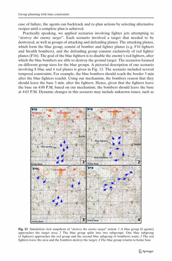
Embedding planning systems in real-world domains is a challenging problem that haswide-ranging importance and applications [11, 18, 19, 21, 44, 70, 82, 86]. Examplesof these settings are problems that are inherently distributed, such as training andeducational settings, Internet information sharing, interactive entertainment, searchand rescue missions and robotic space missions [44, 82]. Additionally, using multipleagents to create a plan often yields increased performance and task reliability evenin situations where the task can theoretically be performed by a single agent [19].
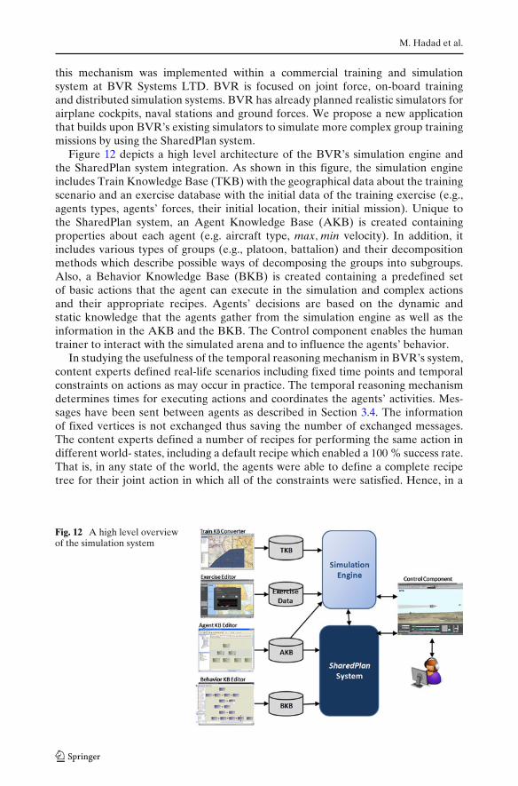
A key challenge in these planning systems is the ability to address real-worlddynamics, typically done through interleaving planning and execution [21]. This typeof planning could potentially address the following types of dynamics: the worldchanges in ways that are beyond the agent’s control; the features of the worldare revealed incrementally; temporal constraints force execution to begin before acomplete plan can be generated; new goals evolve over time [18]. It is impracticalto plan for all possible eventualities in such scenarios, particularly due to the highlydynamic nature of multiple agents systems [70]. Moreover, as planning systems areimplemented in real-world applications, they raise the issue of temporal constraintsin the environments in which they operate [11, 86].
The first contribution of this paper lies in presenting a temporal reasoningmechanism for multiple self-interested planning agents that must coordinate theiractions in order to accomplish a joint action under temporal constraints. The mech-anism utilizes a temporal constraint network technique to guarantee the temporalconsistency of a cooperative plan. The major novelty of the reasoning mechanism isits integration within a distributed planning system based on a well-grounded BDItheoretical model of cooperation, namely the SharedPlan [26] model. SharedPlan
Group planning with time constraints
is generally used to define essential characteristics of teamwork for supporting thedesign and construction of collaborative systems. This includes allowing agents in agroup to plan a joint action, perform the action or carry out activities in order to helpfacilitate their cooperative plan.
This paper also contains two key contributions about how the BDI model isimplemented, which are equally applicable for cases of selfless or self-interestedagents. First, we present how abstraction can be used to implement teamwork,allowing for joint action to be defined without explicitly describing all possible statesin advance, as is done in former frameworks of teamwork [41, 82], making it possibleto reduce the number of states which need to be considered.1 Second, as each agentmay reason by itself about the best time to perform its activities, the mechanismreduces coordination messages among the group members. Keeping the search spaceas small as possible is critical for implementing a working application, especially onecapable of running in real-time even as it handles dynamics. Keeping the number ofmessages small is important for environments where communication is costly, noisyor otherwise problematic.
Applying our mechanism in a real-world application raises new questions regard-ing the order of plan generation and the commitment of the group to partial plans.We discuss these questions in the next sections and explore them by implementingdifferent methods in a synthetic rescue environment. The results demonstrate thatfor environments which we have tested, it is better to commit as late as possible.Furthermore, when group members use a similar order to plan parts of their jointaction, they have a better chance of succeeding in finding a cooperative plan thatsatisfies all of the temporal constraints. We have implemented the mechanism as apart of the SharedPlan system and integrated it within a military commercial trainingand simulation application. The mechanism enables the successful simulation of real-life scenarios where a group of agents has to jointly achieve military missions undertemporal constraints. We present empirical evidence for the effectiveness of themechanism in reducing communication to coordinate the group members’ activities.
This work is strongly based on the SharedPlan framework [26]. In Section 2,we briefly describe this framework. In Section 3 we provide formalization oftemporal constraint networks in the context of the SharedPlan. Then, we presentthe temporal reasoning algorithm including methods for exchanging and mergingtemporal information among the group members. The algorithm ensures temporalconsistency of the plans, determines times for executing actions, and coordinates theagents’ activities in such a way that all of the temporal constraints are satisfied. InSection 4 we prove the correctness of the temporal reasoning algorithm and discussits complexity. In Section 5 we discuss methods for exchanging and merging temporalinformation among the agents, and we study the behavior of these methods in asynthetic rescue environment. An additional problem that we explore relates tothe order in which the group members should plan the subsidiary actions of theirjoint activity. In this section we also discuss how the mechanism was successfullyimplemented within a commercial training and simulation system for a militarydomain. In Section 6, we survey related research fields on planning systems withtemporal reasoning and scheduling and compare them with our work. Finally, inSection 7, we conclude and present possible directions of future research.
1The empirical evidence is beyond the scope of this paper and can be found at [32].
M. Hadad et al.
2 Overview of the SharedPlan model
In this section we overview basic concepts and planning processes of the theoreticalSharedPlan model [26]. We then describe the major component of the SharedPlansystem which we developed in [29] that we use in this paper. To motivate thediscussion we start with an informal example of “rescue disaster survivors” by tworescue robots. We refer to this example throughout the paper.
2.1 A motivating example
Assume two rescue robots A1 and A2 must jointly perform the action “rescue disastersurvivors” denoted by α. Suppose that A1 and A2 have different capabilities. RobotA1 is small and flexible and is able to maneuver deep into crevices in the rubble,flatten itself to crawl through tight spaces, or rear up to climb and look over objects.The second robot, A2, is large and strong. It is designed to pick up concrete slabs,pipes, broken boards, etc., in the collapsed area. Thus, A1 and A2 must collaborateon some activities in order to succeed in performing action α. Robots A1 andA2 may have various temporal constraints. For instance: A1 and A2 arrive at thecollapsed area at 4:00 P.M.; the batteries of A2 are restricted for 150 min.; A1 andA2 must finish the joint action by 7:30 P.M. In this paper we wish to address queriessuch as: “When should A1 inform A2 that it has completed its activities?”; “Whichtemporal information do A1 and A2 exchange?”; “Which robot checks the temporalconsistency of a joint action?”; “Can the robots complete their activities on time, ordo they perhaps need some help?”, and so on.
Consider in the previous example that A1 and A2 have agreed to the follow-ing plan in order to perform action α, “rescue disaster survivors”: Suppose thataction α is divided into subactions β1, β2, . . . , β5 which are respectively defined asfollows: “f ind and identify the victims in area A”, “f ind and identify the victimsin area B”, “clear obstructions blocking doorways in area A”, “rescue the victimsoutside the building in area A” and “rescue the victims outside the building in areaB”. Also assume that they divide the responsibility among themselves as follows: A1
performs subactions β1, β2, β4 and β5, and A2 performs subactions β3, β4 and β5. Notethat some subactions are performed by a single agent and others (i.e., β4 and β5) aremulti-agent actions that require cooperation between A1 and A2.
These subactions may include several “precedent constraints”. For example, as-sume that A2 must know the location of the “victims” before it begins to clearblocked doorways in the area (i.e., β1 must be carried out before β3). Also, sincearea B is less dangerous than area A, area B will be scanned by A1 only after areaA is scanned (i.e., β1 will be performed before β2). In addition, they will “rescue thevictims outside the building in area A” only after A2 clears the blocked doorways inarea A (i.e., β3 will be performed before β5), and after A1 “f inds and identif ies thevictims in area B” (i.e., β2 will be performed before β4). They will “rescue the victimsoutside the building in area B" after A1 “f inds and identif ies the victims in area B”(β2 is performed before β5).
The directed graph of Fig. 1 illustrates the precedence relations between subac-tions β1, β2, . . . , β5 above. We denote the start and finish time of action βi by thevariables sβi and fβi , respectively, and they are represented as vertices in the graph.Note that agent A2, for example, cannot perform β3 without knowing the finish timeof β1 (because β1 precedes β3).
Group planning with time constraints
Fig. 1 An example of aprecedence graph formulti-agent action α; time(βi)
within which βi must begin andfinish; sβ j and fβ j are variablesrepresenting start and finishtime points of β j, respectively;delayij is the interval thatdenotes a possible delaybetween the finish time ofaction βi and the start time ofaction β j
time(β1)
time( )time( )2
time( )β5time( )β4
β
delay
12
2425
delaydelay35
delay delay13
3β
s
s
β1
β1
β2
β2 β3
β3
f
f f
β4
β4f fβ5
β5
s
ss
A
A 1
2
This example raises the following key questions: At what stage should an agentcommit to a time for performing an action, and inform the rest of the group membersof its commitment? If the individual agent commits to a specific time early on andannounces this commitment to the other agents, it may need to negotiate with theother agents if it needs to change its schedule later. Alternatively, if the commitmentis made and announced as late as possible, e.g., only when requested by other groupmembers, it may delay the other group members’ planning. Another question refersto the order in which each individual in the group plans its subactions in the jointplan and identifies the values of the time variables. For example, suppose that thereis no precedent relation between β1 and β2. Then, A1 can either plan β1 before β2 orvice versa. We explore these questions empirically in Section 5.1.
2.2 Basic definitions of a collaborative plan
In this section we briefly describe basic definitions of the SharedPlan model that arethe formal basis of the temporal reasoning mechanism. The definitions are based onthe original formalization but augmented to include time constraints in an explicitway. The planning approach contains many similarities to the previous HierarchicalTask Network (HTN) [23, 25, 37, 65] but includes extensions for joint action planningin a multi-agent environment.
An action, in the model, is an abstract entity which has various propertiesassociated with it such as action type, agent, time of performance, and other objects
M. Hadad et al.
involved in performing the action. An action may be either a basic action or acomplex action. A basic action is an action that can be directly executed by the agentand cannot be subdivided into subactions (e.g., crawl, look over objects, pick-up).A (higher-level) complex action is one that cannot be executed directly and is de-composed into subactions (e.g., find and identify the victims). In addition, an actionmay be either a single-agent action or a multi-agent action. A single-agent actioncan be executed by a single agent and a multi-agent action requires two or morecooperative agents to complete the action jointly. To execute a high-level complexaction the agents must identify a recipe for it. They may know several recipes for thesame action. The model assumes that each agent has a library of recipes. A recipefor action α, denoted by Rα , refers to a set of actions, which we denote by βi (1 ≤i ≤ n), and appropriate constraints, denoted by ρ j (1 ≤ j ≤ m), specifying how theactions can be performed and which agents can perform which action. A constraintρk, contains variables Xi defined in a certain domain Domi. Examples of recipeconstraints are agents constraints, precedence constraints and metric constraints. Theagents constraints specify the capabilities that are required of the agents to performspecific actions in the recipe. For example, the number of agents required to performan action in a recipe may be between 2 and 5—or formally, 2 ≤ XagentNun ≤ 5.Alternatively, these constraints may specify the type of agent that can perform acertain action, e.g., the agent must be a small robot. Precedence constraints referto the execution order of the actions. Metric constraints indicate specific times forexecuting actions in the recipe.
In order to perform some complex action βi, the agents have to identify arecipe Rβi for it. There may be several recipes for βi. The recipe Rβi may includesubactions δiv . Each δiv may similarly be either basic or complex. An illustration ofdecomposition of α when the plan is fully initiated is depicted in a complete recipe treefor α of agent Ak. Formally, recipe tree for α of agent Ak is represented by an acyclicdigraph Tk
α = (Vkα, Ek
α) in which Vkα is the nodes set, Ek
α is the edge set, and eachnode v ∈ Vk
α contains an action. We assert that Tα = (V1α ∪ . . . ∪ Vn
α, E1α ∪ . . . ∪ En
α)
is the union recipe tree of a group of agents Aα = {A1, . . . , An} that jointly execute amulti-agent action α.
Figure 2 demonstrates an example of possible recipe trees for the action “rescuedisaster survivors” in a specific world-state. The bold edges represent the actionsperformed by both robots and the dashed edges are the actions performed by asingle agent (A1, or A2). The trees differ with respect to single-agent actions butare identical with respect to the first level of each multi-agent action. For example,action α is a multi-agent action and must be performed by A1 and A2; thus, the treesof both robots consist of the first level of α (i.e., β1, . . . , β5). On the other hand, β1
is a single-agent action which has to be performed by A1; thus, A2 does not knowabout actions γ11 and γ12 which are selected by A1 in order to perform action β1.Similarly, β3 has to be performed by A2 and thus A1 does not know about A2’s planto perform β3.
The SharedPlan formalism proposes several collaborative planning processes toidentify a plan for a joint action α. The formalism distinguishes between five differenttypes of plans. A full individual plan specifies those conditions under which an indi-vidual agent can be said to have a fully initiated plan to perform a single-agent ac-tion α. A partial individual plan deals with both partiality of knowledge and partialityof intention. A SharedPlan representing that a group of agents has a collaborative
Group planning with time constraints
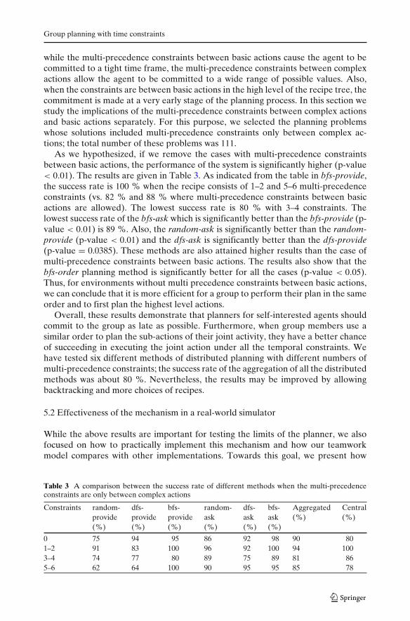
Fig. 2 Part of possible recipe trees for the action “rescue disaster survivors”, the top tree is plannedby the large robot and the bottom is planned by the small robot. The dashed edges representindividual plans. The gray boxes represent basic actions.
plan to perform together some action α is defined recursively in terms of a fullSharedPlan and a partial SharedPlan. A full SharedPlan is the collaborative correlateof a full individual plan and includes full individual plans among its constituents. Apartial SharedPlan is the collaborative correlate of a partial individual plan. A prin-cipal way in which the SharedPlan differs from the individual plan is that knowledgeabout how to act, ability to act and commitment to act are distributed in theSharedPlan.
The SharedPlan model presents several planning processes for the individual andgroup to expand partial plans into more complete ones. Even though all of planningprocesses are implemented in the system, in order to simplify the presentation ofthe temporal reasoning mechanism we omit the details. More discussion of theSharedPlan definitions and of the planning processes is given in [26, 27].
2.3 An example of a collaborative plan with time constraints
A collaborative plan of a multi-agent action can be illustrated by the rescue robotsexample introduced above. In this example, a multi-agent action α, “rescue disaster
M. Hadad et al.
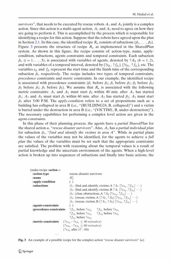
survivors”, that needs to be executed by rescue robots A1 and A2 jointly is a complexaction. Since this action is a multi-agent action, A1 and A2 need to agree on how theyare going to perform it. This is accomplished by the process which is responsible foridentifying a recipe for this action. Suppose that the robots have agreed upon the planin Section 2.1. In this case, the identified recipe Rα consists of subactions {β1, . . . , β5}.Figure 3 presents the structure of recipe Rα as implemented in the SharedPlansystem. As shown in this figure, the recipe consists of: action-type, name, apply-condition, subactions, agents constraints and temporal constraints. Each subactionβi, (i = 1, . . . , 5), is associated with variables of agents, denoted by ?Ak (k = 1, 2),and with variables of a temporal interval, denoted by [?sβ1 , ? fβ1 ], [?sβ2 , ? fβ2 ], etc. Thevariables sβi and fβi represent the start time and the finish time of the correspondingsubaction βi, respectively. The recipe includes two types of temporal constraints,precedence constraints and metric constraints. In our example, the identified recipeis associated with precedence constraints {β1 before β2; β1 before β3; β2 before β4;β2 before β5; β3 before β5}. We assume that Rα is associated with the followingmetric constraints: A1 and A2 must start β4 within 40 min. after A1 has startedβ1; A1 and A2 must start β5 within 60 min. after A2 has started β3; A2 must startβ3 after 5:00 P.M. The apply-condition refers to a set of propositions such as: abuilding has collapsed in area B (i.e., “(BUILDING24, B, collapsed)”) and a victimis buried under the destruction in area B (i.e., “(VICTIM1, B, under-destruction)”).The necessary capabilities for performing a complex level action are given in theagent-constraints.
In this phase of their planning process, the agents have a partial SharedPlan forthe shared action α, “rescue disaster survivors”. Also, A1 has a partial individual planfor subaction β1, “f ind and identify the victims in area A”. While in partial plansthe values of the variables may not be identified, for the agents to achieve a fullplan the values of the variables must be set such that the appropriate constraintsare satisfied. The problem with reasoning about the temporal values is a result ofpartial knowledge and the uncertain environment of the agents. When a high-levelaction is broken up into sequences of subactions and finally into basic actions, the
Fig. 3 An example of a possible recipe for the complex action “rescue disaster survivors” (α)
Group planning with time constraints
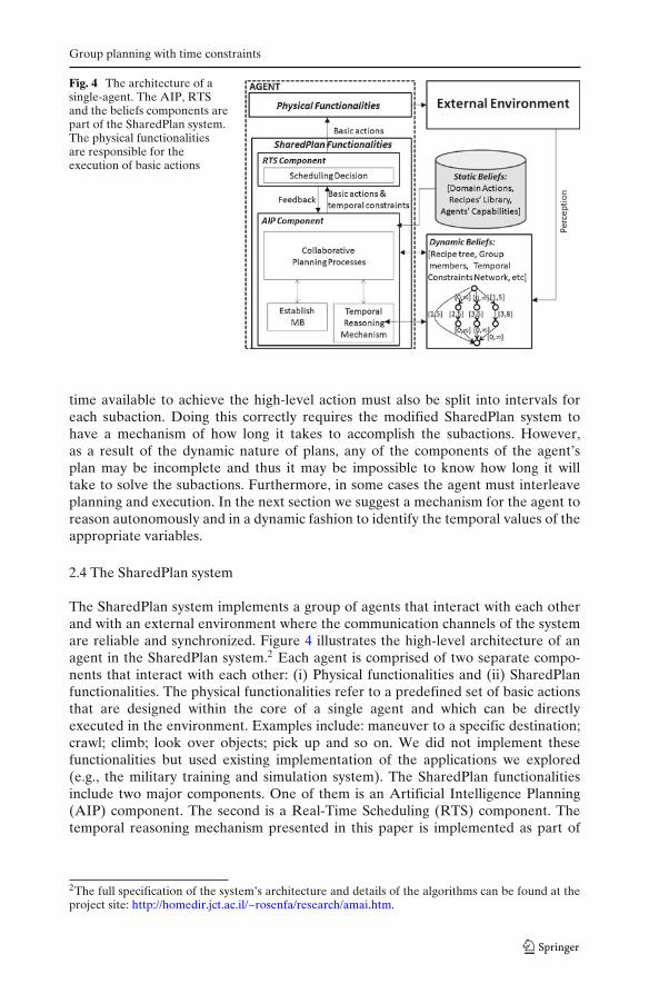
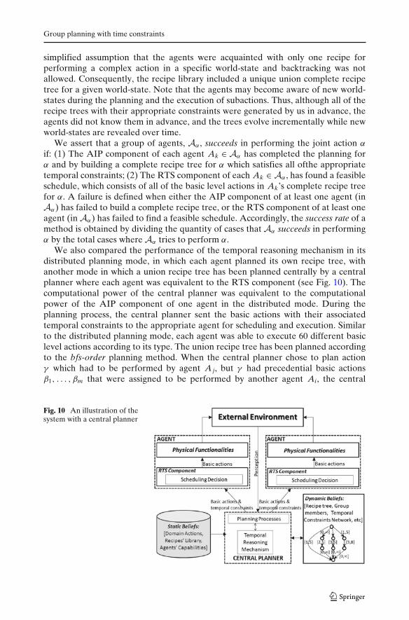
Fig. 4 The architecture of asingle-agent. The AIP, RTSand the beliefs components arepart of the SharedPlan system.The physical functionalitiesare responsible for theexecution of basic actions
time available to achieve the high-level action must also be split into intervals foreach subaction. Doing this correctly requires the modified SharedPlan system tohave a mechanism of how long it takes to accomplish the subactions. However,as a result of the dynamic nature of plans, any of the components of the agent’splan may be incomplete and thus it may be impossible to know how long it willtake to solve the subactions. Furthermore, in some cases the agent must interleaveplanning and execution. In the next section we suggest a mechanism for the agent toreason autonomously and in a dynamic fashion to identify the temporal values of theappropriate variables.
2.4 The SharedPlan system
The SharedPlan system implements a group of agents that interact with each otherand with an external environment where the communication channels of the systemare reliable and synchronized. Figure 4 illustrates the high-level architecture of anagent in the SharedPlan system.2 Each agent is comprised of two separate compo-nents that interact with each other: (i) Physical functionalities and (ii) SharedPlanfunctionalities. The physical functionalities refer to a predefined set of basic actionsthat are designed within the core of a single agent and which can be directlyexecuted in the environment. Examples include: maneuver to a specific destination;crawl; climb; look over objects; pick up and so on. We did not implement thesefunctionalities but used existing implementation of the applications we explored(e.g., the military training and simulation system). The SharedPlan functionalitiesinclude two major components. One of them is an Artificial Intelligence Planning(AIP) component. The second is a Real-Time Scheduling (RTS) component. Thetemporal reasoning mechanism presented in this paper is implemented as part of
2The full specification of the system’s architecture and details of the algorithms can be found at theproject site: http://homedir.jct.ac.il/~rosenfa/research/amai.htm.
the AIP component. The AIP component includes collaborative planning processeswhich we previously discussed.
In addition to the above functionalities, each agent may access the data ofbeliefs. The beliefs may be either static or dynamic. Static beliefs are predefinedand include a library of recipes, description of domain actions, knowledge aboutthe agent capabilities and so on. The recipe tree is a part of the dynamic beliefs asthe agent modifies it during the execution. The beliefs about the states of the othergroup members are also dynamic. The external environment (e.g., the simulator) isdesigned to test the validity of a predefined set of propositions in the agent arena(e.g, ‘is there an obstacle on the left side?’) and to answer a predefined set of queries(e.g., ‘what is the level of my energy?’). The answers are also referred to as dynamicbeliefs.
The AIP component plans the agent’s activities while interacting with the envi-ronment (including other agents). It identifies, incrementally, a set of basic actions,and a set of temporal requirements associated with the basic actions, to perform α
without conflict. During the planning process each basic action β is sent to the RTScomponent, along with its temporal requirements 〈Dβ, dβ, rβ, pβ〉 where Dβ is theDuration time, i.e., the time necessary for the agent to execute β without interruption;dβ denotes the deadline, i.e., the time by which β must be completed; rβ refers tothe release time, i.e., the time at which β is ready for execution; pβ denotes thepredecessor actions, i.e., the set {β j|1 ≤ j ≤ n} of basic actions whose execution mustterminate before beginning β. The RTS component receives the basic actions setwith the associated requirements and inserts these actions into the agent’s scheduleas described in the following section. The RTS component is responsible for thescheduling and dispatching of basic actions for execution. The scheduling problemthat our RTS component faces is NP-hard [24]. We describe the heuristic algorithmwhich is used in the RTS component in [33].
3 Mechanism for group temporal reasoning
We consider a problem where a group of agents Aα = {A1, . . . , An} must jointlyexecute a multi-agent action α. We assume that α is a complex action. The agentsare acquainted with a set of actions (either basic or complex), library of recipes andan initial set of beliefs. We present a mechanism for Aα to identify a full shared planin order to execute α without violating temporal constraints. Each agent in Aα shouldperform its own part in the plan by identifying a set of basic actions along with theirtemporal requirements 〈Dβ, dβ, rβ, pβ〉 and dispatching them for execution underthese requirements. We begin the section with basic definitions. A summary of thenotations used in the temporal reasoning mechanism is given in Table 1.
3.1 Supporting definitions and notations
As described in previous sections, a contribution of this paper is how we modelthe agents’ behavior based on the theoretical SharedPlan model of cooperation yetextend this framework to allow for self-interested agents to plan joint activities withtemporal constraints. A second novel contribution of this papers lies within how weimplemented this extended framework. Specifically, we model dynamics by using
Group planning with time constraints
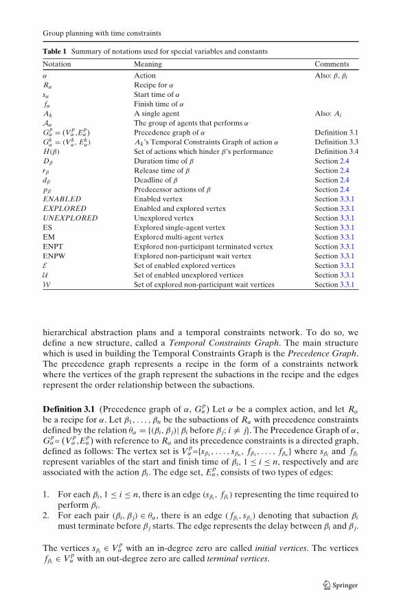
Table 1 Summary of notations used for special variables and constants
H(β) Set of actions which hinder β’s performance Definition 3.4Dβ Duration time of β Section 2.4rβ Release time of β Section 2.4dβ Deadline of β Section 2.4pβ Predecessor actions of β Section 2.4ENABLED Enabled vertex Section 3.3.1EXPLORED Enabled and explored vertex Section 3.3.1UNEXPLORED Unexplored vertex Section 3.3.1ES Explored single-agent vertex Section 3.3.1EM Explored multi-agent vertex Section 3.3.1ENPT Explored non-participant terminated vertex Section 3.3.1ENPW Explored non-participant wait vertex Section 3.3.1E Set of enabled explored vertices Section 3.3.1U Set of enabled unexplored vertices Section 3.3.1W Set of explored non-participant wait vertices Section 3.3.1
hierarchical abstraction plans and a temporal constraints network. To do so, wedefine a new structure, called a Temporal Constraints Graph. The main structurewhich is used in building the Temporal Constraints Graph is the Precedence Graph.The precedence graph represents a recipe in the form of a constraints networkwhere the vertices of the graph represent the subactions in the recipe and the edgesrepresent the order relationship between the subactions.
Definition 3.1 (Precedence graph of α, Gpα) Let α be a complex action, and let Rα
be a recipe for α. Let β1, . . . , βn be the subactions of Rα with precedence constraintsdefined by the relation θα = {(βi, β j)| βi before β j; i �= j}. The Precedence Graph of α,Gp
α= (V pα ,Ep
α) with reference to Rα and its precedence constraints is a directed graph,defined as follows: The vertex set is V p
α ={sβ1 , . . . , sβn , fβ1 , . . . , fβn} where sβi and fβi
represent variables of the start and finish time of βi, 1 ≤ i ≤ n, respectively and areassociated with the action βi. The edge set, Ep
α , consists of two types of edges:
1. For each βi, 1 ≤ i ≤ n, there is an edge (sβi , fβi) representing the time required toperform βi.
2. For each pair (βi, β j) ∈ θα , there is an edge ( fβi , sβ j) denoting that subaction βi
must terminate before β j starts. The edge represents the delay between βi and β j.
The vertices sβi ∈ V pα with an in-degree zero are called initial vertices. The vertices
fβi ∈ V pα with an out-degree zero are called terminal vertices.
M. Hadad et al.
Example 3.1 The gray vertices and edges of the graph in Fig. 5 illustrate thePrecedence Graph, Gp
α , of a possible recipe Rα where V pα = {sβ1 , . . . , sβ5 , fβ1 , . . . , fβ5}
( fβ2 , sβ4), ( fβ2 , sβ5), ( fβ3 , sβ5) }. The vertex sβ1 is an initial vertex, and vertices fβ4 , fβ5
are terminal vertices.
Using a recipe to create the temporal constraints graph forms an abstract hierar-chical structure of a partial plan where several vertices are associated with differentagents. The precedence relationship between subactions which are not associatedwith the same group of agents is called a Multi-Precedence Constraint.
Definition 3.2 (Multi-precedence constraint) A precedence relation “βi before β j”is called a Multi-Precedence Constraint if subactions βi and β j are performed bydifferent groups of agents, i.e. Aβi �= Aβ j .
Example 3.2 As shown in the Precedence Graph Gpα in Fig. 5, actions β1 and β2
are single-agent actions which have to be performed by A1. Similarly, action β3
is a single-agent action which has to be performed by A2. Actions β4 and β5 aremulti-agent actions which have to be performed by A1 and A2 jointly, that is,Aβ4 = {A1, A2} and also Aβ5 = {A1, A2}. The precedence relations: (β1, β3), (β2, β4),(β2, β5) and (β3, β5) are multi-precedence constraints. Agent A2, for example, cannotdecide on the start time of β3 without knowing the temporal requirements of itspreceding action β1, which is planned by A1.
When group Aα works on the action α, each agent Ak ∈ Aα maintains a TemporalConstraints Graph. The definition of the Temporal Constraints Graph is a combi-nation of a temporal constraints network with hierarchical abstraction of a jointplan. Hence, it utilizes the SharedPlan model to provide collaboration, HierarchicalTask Network (HTN) to enable the construction of abstract plans and a networkof binary constraints to enable applying existing techniques in order to resolvetemporal constraints. While we assume that the reader is broadly familiar with
Fig. 5 An example of aTemporal Constraints GraphGk
α , constructed from aPrecedence Graph Gp
α , whichis maintained by an agent Ak
S plan
[
16:00{A1,A2}
SS 1
[0,210]
[0, ]A1
f 1
[0, ]
[0, ][0, ]
{A1,A2}
A
S 2S 3
[0, ][0, ]
[0,210][0,150]
A1 A2A1
f 2f 3
SS[0, ]
[0, ][0, ]A2
A1
54
f
[0, ][0, ]Types of vertices:
{A1,A2}{A1,A2}
f
5f 4 Unexplored
Explored
[0, ]
[0, ]
{A1,A2}{A1,A2}{A1,A2}
Group planning with time constraints
Temporal Constraint Satisfaction Problem (TCSP) [16, inter alia], a description ofour application of this problem is as follows:
Definition 3.3 (Temporal constraints graph of α, Gkα) A Temporal Constraints
Graph Gkα = (Vk
α, Ekα) of an agent Ak is a weighted graph constructed from a
Precedence Graph Gpα= (V p
α ,Epα) where Vk
α = V pα ∪ {sαplan , sα, fα} and sαplan represents
the time point at which Ak starts to plan action α. Ekα consists of the edges Ep
α
∪{(sαplan , sα), (sα, fα), (sαplan , fα)} with additional edges from sα to each initial vertexin Gp
α and from each terminal vertex of Gpα to fα . For any complex subaction βi
which is associated with Gpα= (V p
α ,Epα) and in which Ak participates, the Temporal
Constraints Graph is updated recursively (i.e., Vkα grows to be Vk
α ∪ V pβ i
and Ekα grows
to be Ekα ∪ Ep
β iwith additional edges from sβi to each initial vertex in Gp
β iand from
each terminal vertex of Gpβ i
to fβi ).Each edge in Gk
α is labeled by an interval [a, b ] which denotes an upper and lowerbound on a time gap. If e = (sβi , fβi) then [a, b ] denotes the time gap for the durationrequired to complete subaction βi, and if e = ( fβi , sβ j) then [a, b ] denotes a possibledelay between the end of subaction βi and the beginning of subaction β j. Initially, allof the edges are labeled [0,∞].
Each action β which is associated with any vertex in Vkα contains the following
information: (a) whether β is basic or complex; (b) whether β is a multi-agent or asingle-agent action; (c) whether a plan for β has been completed; (d) whether β hasalready been executed by the agent(s); and (e) the agent(s) that is (are) assigned toperform β.
An example of a Temporal Constraints Graph Gkα , constructed from the Prece-
dence Graph Gpα in Fig. 1, is given in Fig. 5. A more complex example, where
G1α �= G2
α , can be seen in the next sections in Figs. 7 and 8. Each single agent Ak
in the system runs the algorithm independently in order to construct its TemporalConstraints Graph Gk
α . The information maintained by the graph is determinedincrementally by the algorithm which also expands the graph.
In Section 2.2 we defined the recipe trees for action α (see an illustration in Fig. 2).This definition was formed by Definition 3.1 of Precedence Graph and Definition 3.3of Temporal Constraints Graph. We note that given the Temporal Constraints Graphthe recipe tree is implicit in the graph and can be easily derived. Thus, similar torecipe trees, the graph of each individual agent in Aα may be different with respect toits individual actions, but similar with respect to the first level of multi-agent actions.
As mentioned above, in several cases Aβ ’s members are not able to complete β’splan without receiving relevant information about the actions preceding β from theagents performing them. The set of these preceding actions hinders the performanceof β; this set is denoted H(β). More formally:
Definition 3.4 Hinder members of an action β j, H(β j), are defined as the set of allminimal members3 of the set {βi|βi precedes β j and Aβ j � Aβi}.
3We recall that v is a minimal member of S in a partial order if v ∈ S and no other w ∈ S exists suchthat w precedes v. Note that a minimal member is not unique.
M. Hadad et al.
3.2 General description of the temporal reasoning algorithm
The Temporal Reasoning Algorithm is used by each Ak ∈ Aα . The pseudocode isgiven in Fig. 6. In the initialization phase Ak constructs its initial Gk
α . Then, in theplanning and executing loop, Ak expands its Gk
α recursively according to
Fig. 6 The Temporal Reasoning Algorithm for identifying values for temporal variables which is runby each agent Ak ∈ Aα during the performance of α
Group planning with time constraints
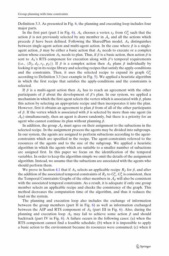
Definition 3.3. As presented in Fig. 6, the planning and executing loop includes fourmajor parts.
In the first part (part I in Fig. 6), Ak chooses a vertex sβ from Gkα such that the
action β is not previously selected by any member in Aα and all the actions whichprecede β have been defined. Following the SharedPlan model, Ak distinguishesbetween single-agent action and multi-agent action. In the case where β is a single-agent action, β may be either a basic action that Ak needs to execute or a complexaction whose execution Ak needs to plan. Thus, if β is a basic action, then action β issent to Ak’s RTS component for execution along with β’s temporal requirements(i.e., 〈Dβ, dβ, rβ, pβ〉). If β is a complex action then Ak plans β individually bylooking it up in its recipe library and selecting recipes that satisfy the apply-conditionsand the constraints. Then, it uses the selected recipe to expand its graph Gk
α
according to Definition 3.3 (see example in Fig. 5). We applied a heuristic algorithmin which the first recipe that satisfies the apply-conditions and the constraints isselected.
If β is a multi-agent action then Ak has to reach an agreement with the otherparticipants of β about the development of β’s plan. In our system, we applied amechanism in which the first agent selects the vertex which is associated with β, plansthis action by selecting an appropriate recipe and then incorporates it into the plan.However, first it obtains an agreement to plan β from of all of the other participantsof β. If the vertex which is associated with β is selected by more than one agent (inAβ) simultaneously, then an agent is drawn randomly, but there is a priority for anagent who cannot continue its plan without planning β.
In addition, the group Aβ must agree on their assignment to the subactions in theselected recipe. In the assignment process the agents may be divided into subgroups.In our system, the agents are assigned to perform subactions according to the agent-constraints which are specified in the recipe. The agent-constraints referred to theresources of the agents and to the size of the subgroup. We applied a heuristicalgorithm in which the agents which are suitable to a smaller number of subactionsare assigned first. In this paper we focus on the identification of the temporalvariables. In order to keep the algorithm simple we omit the details of the assignmentalgorithm. Instead, we assume that the subactions are associated with the agents whoshould perform them.
We prove in Section 4.1 that if Ak selects an applicable recipe Rβ for β, and afterthe addition of the associated temporal constraints of Rβ to Gk
α , Gkα is consistent, then
the Temporal Constraints Graphs of the other members in Aβ will also be consistentwith the associated temporal constraints. As a result, it is adequate if only one groupmember selects an applicable recipe and checks the consistency of the graph. Thismethod decreases the computation time of the algorithm, and thus it reduces theload on the system.
The planning and execution loop also includes the exchange of informationbetween the group members (part II in Fig. 6) as well as information exchangedbetween the AIP and RTS component of Ak (part III in Fig. 6). Also, during theplanning and execution loop Ak may fail to achieve some action β and shouldbacktrack (part IV in Fig. 6). A failure occurs in the following cases: (a) when theRTS component cannot find a feasible schedule; (b) when it is impossible to applya basic action to the environment because its resources were consumed; (c) when it
M. Hadad et al.
is impossible to apply a selected recipe to the environment because of unexpectedchanges; (d) when its group members abandon the joint action. The backtrackingmechanism is beyond the scope of this paper.
3.3 The temporal reasoning algorithm
In the following sections we describe in detail the algorithm in Fig. 6 and then wedemonstrate the algorithm’s operation using the rescue robots example.
3.3.1 Def inition and initialization
In the main procedure, agent Ak receives action α along with the group Aα asan input. The Temporal Constraint Graph is initialized (line 1 in Fig. 6) as wellas some variables of the algorithm. The boolean variables b IsFinishedExecuteAll,b IsCompletedPlan and b IsFailureInPlan denote whether all of the basic actionsassociated with Ak have been executed and the status of the joint plan respectively.Initially, all of the vertices are UNEXPLORED (line 3 in Fig. 6). There are fourtypes of EXPLORED vertices as follows:
1. A vertex of a single-agent action which is performed by Ak becomes ExploredSingle-agent (ES).
2. A vertex of a multi-agent action in which Ak participates becomes ExploredMulti-agent (EM).
3. A vertex with unknown temporal values of an action in which Ak does notparticipate becomes Explored Non-Participant Wait (ENPW). In this case Ak
waits until it receives the temporal values of the vertex from an appropriateagent.
4. A vertex with known temporal values of an action in which Ak does notparticipate becomes Explored Non-Participant Terminated (ENPT).
A vertex which is associated with an action which temporal values can be defined(because the temporal values of all of its predecessors have been defined) is calledan ENABLED vertex. We distinguish between two disjointed sets of ENABLEDvertices: The first set, denoted by U , contains the UNEXPLORED vertices, i.e., thevertices which values can be identified but which the algorithm has not yet handled.The second set, denoted by E , contains the EXPLORED vertices, i.e., the verticeswhich values have been identified. According to the algorithm, a vertex u ∈ Vk
α
becomes ENABLED when the status of all of the preceding vertices of u becomesEXPLORED but not ENPW. All of the vertices that are denoted as ENPW (i.e.,the agent waits to receive the values of their temporal variables from others) aremaintained in the set W .
A vertex associated with a specific time point is called a f ixed vertex. Initially,vertex sαplan is a fixed vertex and is denoted as EM (line 4 in Fig. 6). Then, theU and E sets are updated recursively by an appropriate procedure which is calledupdate_enabled_set and is described in Fig. 17 of Appendix B. In Section 4.1 weprove that there is no deadlock in the system. Hence, at each stage of the algorithmthere is at least one agent which may select an UNEXPLORED vertex from U . Note
Group planning with time constraints
that, in the initialization phase, U set contains the ENABLED vertex sα . Thus, eachagent in Aα starts its execution and planning loop from sα .
3.3.2 Planning for a chosen action
During the planning process, a vertex sβ is selected to be planned by Ak if sβ isan ENABLED vertex and an UNEXPLORED vertex, i.e., sβ is selected from theUNEXPLORED (U) set (line 9 in Fig. 6). For this selected vertex which is associatedwith action β, Ak checks the agents who can participate in the performance of β. Inthe case that Ak does not participate in β’s performance (lines 10–17 in Fig. 6), ifthe temporal values of β are unknown, it changes the status of the vertices sβ and fβto ENPW and adds the vertex sβ to W set (lines 12–14 in Fig. 6). Then, it attemptsto select a new ENABLED vertex from the U set. If its U set is empty but its W isnot empty, it waits for a message with temporal information from the other groupmembers which will allow it to change the status of some ENPW vertices to ENPTvertices and to update its U set. If Ak does not participate in β’s performance but thevalues of β are already known to Ak, it changes the status of the vertices sβ and fβ toENPT and then it updates its U set (lines 15–16 in Fig. 6).
Assume that the selected ENABLED vertex is associated with an action β
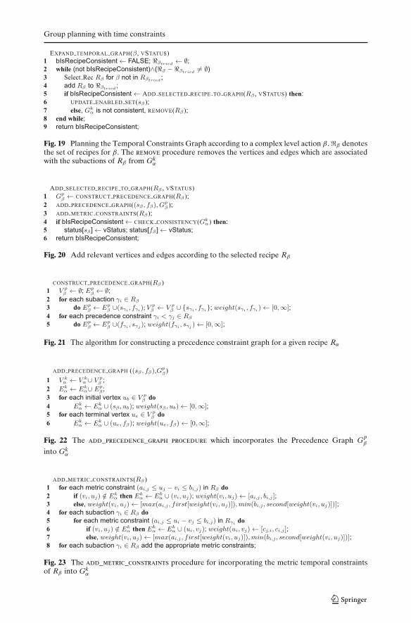
where Ak participates in β’s performance (lines 18–25 in Fig. 6). If Ak is the onlyperformer of this action then Ak distinguishes between basic actions and complexactions (the pseudocode is given in Figs. 19 and 24 in Appendix B, respectively).After Ak completes the planning of β’s plan, if β is a subaction in a recipe of amulti-agent action, it should send information to its group members by running thecheck_necessity_to_update_members procedure (see Fig. 25 in Appendix B). Thegoal of this procedure is to determine whether β is a subaction in a recipe of a multi-agent action and whether β is in a set of the hinder members of some action βi
(i.e., β ∈ H(βi), see Definition 3.4). If β ∈ H(βi), the procedure checks if all othervertices in H(βi) are EXPLORED but not ENPW. If so, the temporal informationof β can be sent to the performers of βi. The methods for exchanging informationare discussed in Section 3.4. In the case where β is a multi-agent action and Ak
is one of the participants (lines 26–27 in Fig. 6), Aβ ’s members have to reach aconsensus on the recipe for β as described in Fig. 18 in Appendix B. Note that theSelect_agreeable_recipe procedure includes a process for selecting a recipe by thegroup Aβ and a process for the assignment of the agents to subactions according tothe SharedPlan model.
3.3.3 An illustration of the temporal reasoning algorithm
In Sections 2.1 and 2.3 we described an example from the rescue domain. In thissection we illustrate the algorithm using that example. The rescue robots A1 andA2 intend to perform a multi-agent action α (i.e., “rescue disaster survivors”) jointly.Suppose that A1 and A2 arrive at the disaster area at 4:00 P.M. Thus, both robotssimultaneously begin the collaborative plan for α. Hence, planning and executing α
begin after 4:00 P.M. Suppose that the batteries of A2 are restricted to 150 min.; thusα must be completed within 150 min. We also assume that α must be finished beforesunset, at 7:30 P.M. Thus, A1 and A2 construct their Temporal Constraints Graphaccordingly (see the bold edges in Fig. 5 in Section 3.1).
M. Hadad et al.
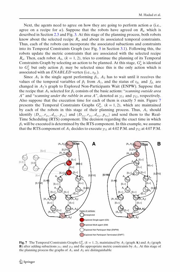
Next, the agents need to agree on how they are going to perform action α (i.e.,agree on a recipe for α). Suppose that the robots have agreed on Rα which isdescribed in Section 2.3 and Fig. 3. At this stage of the planning process, both robotsknow about the selected recipe Rα and about its associated temporal constraints.Thus, each of the robots can incorporate the associated subactions and constraintsinto its Temporal Constraints Graph (see Fig. 5 in Section 3.1). Following this, therobots update the metric constraints that are associated with the selected recipeRα . Then, each robot Ak, (k = 1, 2), tries to continue the planning of its TemporalConstraints Graph by selecting an action to be planned. At this stage, G1
α is identicalto G2
α but only action β1 may be selected since this is the only action which isassociated with an ENABLED vertex (i.e., sβ1 ).
Since A1 is the single agent performing β1, A2 has to wait until it receives thevalues of the temporal variables of β1 from A1, and the status of sβ1 and fβ1 arechanged in A2’s graph to Explored Non-Participants Wait (ENPW). Suppose thatthe recipe that A1 selected for β1 consists of the basic actions: “scanning outside areaA” and “scanning under the rubble in area A”, denoted as γ11 and γ12, respectively.Also suppose that the execution time for each of them is exactly 5 min. Figure 7presents the Temporal Constraints Graphs Gk
α, (k = 1, 2), which are maintainedby each of the robots in this stage of their planning process. Thus, A1 shouldidentify 〈Dγ11 , rγ11 , dγ11 , pγ11〉 and 〈Dγ12 , rγ12 , dγ12 , pγ12〉 and send them to the Real-Time Scheduling (RTS) component. The decision regarding the exact time in whichβ1 will be executed is determined by the RTS component. In this example, we assumethat the RTS component of A1 decides to execute γ11 at 4:02 P.M. and γ12 at 4:07 P.M.
S plan
[0,210]
{A1,A2} 16:00
S
S 1
{A1,A2}
[0, ]
[60 ]
f 1
S 1
[0, ]
[0, ][0, ]A
A1[60, ]
S 2S 3
[0, ][0, ]
[0,210]
[0,150]
A1A2
A1
[0,40]
f 2f 3
SS[0, ]
[0, ][0, ]A2
A1 [0,60]
54
5f 4
[0, ][0, ]
{A1,A2}{A1,A2}
f
f {A1,A2}{A1,A2}
{A1,A2}
[0, ][0, ]
S plan
[0,210]
{A1,A2} 16:00
S
S 1A1
{A1,A2}
[0, ]
1
f 1
[0, ]
[0, ][0, ][0 150] A
[60, ]
S 2S 3
[0, ][0, ]
[0,210][0,150 A1A2
A1
[0,40]
f 2f 3
SS[0, ]
[0, ][0, ]A2
A1 [0,60]
54
f 5f 4
[0, ][0, ]
{A A }
{A1,A2}{A1,A2}
f
f 5f 4 {A1,A2}{A1,A2}
{A1,A2}
[0, ][0, ]Types of vertices:
Unexplored
Explored Multi-agent (EM)
Explored Single-agent (ES)
Explored Not Participant Terminated (ENPT)
Explored Not Participant Wait (ENPW)
A B
Fig. 7 The Temporal Constraints Graphs Gkα , (k = 1, 2), maintained by A1 (graph A) and A2 (graph
B) after adding subactions γ11 and γ12 and the appropriate metric constraints by A1. At this stage ofthe planning process the graphs of A1 and A2 are distinguishable
Group planning with time constraints
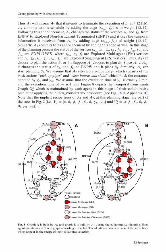
Thus A1 will inform A2 that it intends to terminate the execution of β1 at 4:12 P.M.A1 commits to this schedule by adding the edge (sαplan , fβ1) with weight [12, 12].Following this announcement, A2 changes the status of the vertices sβ1 and fβ1 fromENPW to Explored Non-Participant Terminated (ENPT) and it uses the temporalinformation it received from A1 by adding edge (sαplan , fβ1) of weight [12, 12].Similarly, A1 commits to its announcement by adding this edge as well. In this stageof the planning process the status of the vertices sαplan , sα, fα, sβ1 , fβ1 , sγ11 , fγ11 , sγ12 andfγ12 are EXPLORED, where sαplan , sα, fα are Explored Multi-agent (EM) verticesand sβ1 , fβ1 , sγ11 , fγ11 , sγ12 , fγ12 are Explored Single-agent (ES) vertices . Thus, A1 canchoose to plan the action β3 or β2. Suppose A1 chooses to plan β3. Since A1 /∈ Aβ3 ,it changes the status of sβ3 and fβ3 to ENPW and it plans β2. Similarly, A2 canstart planning β3. We assume that A2 selected a recipe for β3 which consists of thebasic actions “pick up pipes” and “clear boards and slabs” which block the entrance,denoted by γ31 and γ32. We assume that the execution time of γ31 is exactly 2 min.and the execution time of γ32 is 1 min. Figure 8 depicts the Temporal ConstraintsGraph Gk
α which is maintained by each agent in this stage of their collaborativeplan after applying the check_consistency procedure (see Fig. 16 in Appendix B).Note that the implicit recipe trees of A1 and A2, at this planning stage, are part ofthe trees in Fig. 2 (i.e., V1
Fig. 8 Graph A is built by A1 and graph B is built by A2 during the collaborative planning. Eachagent maintains a different graph according to its plan. The identical vertices represent the subactionswhich appear in the recipe of their collaborative action
M. Hadad et al.
3.4 Information exchange between agents
Identification of values for temporal variables in the collaborative plan for α requiresinformation exchange. Each Ak ∈ Aα exchanges information with its group membersin the following cases:
(1) When they identify a recipe for their joint action or for any joint subaction intheir plan. This exchange of messages may be about possible recipes and mayalso be part of their group decision-making.
(2) Agent Ak may inform its group members about completing the plan of asubaction in a recipe of a joint action. It informs the group members that itsplan for their joint action has been completed.
(3) Agent Ak may inform its group members about the time values that it identifiedfor the set H(γ ) of individual actions which hinder γ (see Definition 3.4).
(4) When agent Ak finishes the execution of all of the basic level actions in itscomplete recipe tree it informs the group members.
(5) If Ak has already sent information to specific group members about some actionβ but failed to perform it, then Ak backtracks and informs them about thefailure of β or about the changes in their plan that were determined as a resultof the backtracking.
The information exchange in case (1) above, is done in the select_agreeable_recipe (β) procedure (lines 26–27 in Fig. 6). It refers to their agreement on the recipeselection and the assignment to subactions. The information exchanges in cases (2)–(4) are done in part II of the algorithm (lines 32–33 in Fig. 6). The last case is a caseof failure (line 44 in Fig. 6) where the agent may announce failure or replan actions.Note that replanning of actions causes changes in the recipe tree as well as in theTemporal Constraints Graph.
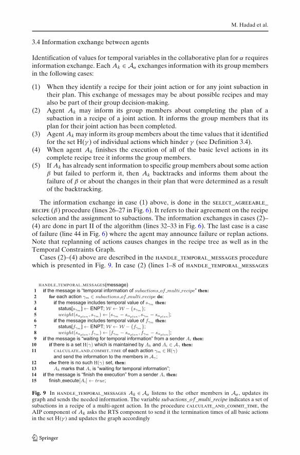
Cases (2)–(4) above are described in the handle_temporal_messages procedurewhich is presented in Fig. 9. In case (2) (lines 1–8 of handle_temporal_messages
Fig. 9 In handle_temporal_messages Ak ∈ Aα listens to the other members in Aα , updates itsgraph and sends the needed information. The variable subactions_of _multi_recipe indicates a set ofsubactions in a recipe of a multi-agent action. In the procedure calculate_and_commit_time, theAIP component of Ak asks the RTS component to send it the termination times of all basic actionsin the set H(γ ) and updates the graph accordingly
Group planning with time constraints
procedure), Ak receives temporal information from its group members. Thus, Ak
changes the relevant vertices in its Temporal Constraints Graph to ENPT. The goalof this message is to enable the agents to know what the status of their joint planis. The joint plan is completed when all of the vertices in the graphs of all of thegroup members have been EXPLORED but not ENPW. In case (3), Ak may beasked about the temporal information (lines 9–13 of handle_temporal_messagesprocedure). Once Ak sends the temporal values of γ1, . . . , γm to its group membersit commits to these values. Thus, one of the main questions in a distributed planningenvironment is at what stage should Ak inform its group members about the timesit will take to perform γ1, . . . , γm, thus committing itself to these times. We considertwo methods of answering this question.
In the first method, called provide-time, Ak sends the temporal information to itsgroup members immediately when it completes the planning of all of the actions thatdirectly precede γ that has to be performed by its group. Thus, Ak should commit tothe temporal values it sends. This method enables the other group members to beginplanning γ immediately upon completion of the planning of all actions precedingaction γ . Furthermore, they do not need to ask each other for the relevant timessince they are informed about them as soon as possible. However, since Ak has tocommit to these times it has less flexibility in determining the time performancefor its other actions. Having flexibility means that an individual agent has morealternatives to change temporal values while it does not need to coordinate thechanges with the other group members. On the contrary, the flexibility is reducedwhen an agent decides to change the announced temporal values and it needs tonegotiate with its group members. Thus, we also consider an alternative mechanism,called ask-time. Following this approach, each member plans its individual actionsas long as it does not depend on its group members’ activities. When such a caseoccurs, the relevant member asks for the appropriate time values from its groupmembers (lines 8–12 of handle_temporal_messages procedure). In this manner, thecommitment is left to the latest time possible, but it may delay the agent waiting foran answer to plan its actions and this method results in additional messages beingexchanged.
3.5 Group planning order
An additional problem in a distributed planning environment involves the order inwhich the members of the group should plan the joint action. As described above,during the planning process, each agent Ak in the group selects a vertex sβ in Gk
α to beexpanded. Vertex sβ is selected by Ak only if it satisfies certain conditions. However,since in most cases there is more than one vertex that satisfies all the requiredconditions, the agent has to decide which of them to select in order to completeits plan. There are several possible selection methods. In the environment that weconsider, the order of the vertices selection may affect Ak’s decision regarding thetime scheduling of its activities. In a joint activity a selection of a specific vertex byan individual agent may influence the activity of the entire group. For instance, incertain cases group members may need temporal information about a specific actionfrom another agent Ak. But the order in which Ak chooses to complete the plan ofthis action may influence the temporal information that it will eventually send andwhen this information will be available.
M. Hadad et al.
In this work we consider three methods for determining the planning order of anindividual in the group. The first is called random-order, where Ak randomly selectsone of the several actions that can be planned. In the second method, called dfs-order, Ak selects the action according to the depth-first search order of Gk
α . In thisorder, the agent selects an action from the lowest level of its recipe tree. Thus, itplans a subaction until it reaches the basic action level, then it continues to the nextsubaction. The third is called bfs-order, where Ak selects one of the actions accordingto the breadth-first search order of Gk
α . In this order, the agent tries to complete theplans of the highest level actions in each stage of the planning process of its recipetree. Note that in the first method the planning order of the group members differ.In the two latter methods, all of the agents in the group plan their subactions in thesame order. Forcing all of the group members to plan subactions in the same ordermay decrease the flexibility of the individuals, but planning the activities in differentorders may delay the plans of some members of the group. Our simulation results,presented in Section 5.1, demonstrate that the planning order influences the successrate of the agents. We show that it is better to commit as late as possible, and thusthe bfs-order and ask-time methods perform the best.
4 Correctness and complexity of the temporal reasoning algorithm
In this section we present the correctness of the temporal reasoning algorithm forspecial cases and discuss its complexity. First, we present lemmas and propositionsto prove that no deadlocks occur and that the algorithm always terminates. Then,we show the cases of soundness and completeness. The termination of the algorithmalso depends on the following cases: (a) the agreement of the group members toperform the selected recipe; (b) the method used to assign group members to performthe subactions; and (c) other constraints associated with the selected recipe. In ourproofs we assume that the members always agree to perform the recipes that satisfythe temporal constraints as well as to perform the subactions that are associated withthem. Also, the recipe does not include additional constraints, except for temporalconstraints. That is, in our proofs we focus on the consistency of the temporalconstraints in the plan.
4.1 Lemmas and propositions
In each stage of the algorithm, Ak selects a vertex v which is an ENABLED vertexand tries to identify its temporal value. In the following proposition we prove that,according to the algorithm, the temporal information of the selected vertex can beidentified and that this vertex is therefore ENABLED.
Proposition 4.1 Suppose that the AIP component of an agent Ak runs the TemporalReasoning Algorithm, which builds the Temporal Constraints Graph Gk
α = (Vkα, Ek
α).Let v be a vertex in Vk
α and S be the set of all minimal members4 of the set {u|u is a
4We recall that v is a minimal member of S in a partial order if v ∈ S and no other w ∈ S exists suchthat w precedes v.
Group planning with time constraints
f ixed vertex and u precedes v}. Then, during the building of the Temporal ConstraintsGraph, if each vertex in the path from all the vertices in S to v are EXPLORED (butnot ENPW), then v is ENABLED.
Proof By induction (see Appendix A).
In the following proposition we prove that all of the values of the variablesassociated with the basic actions which are sent by Ak to its RTS component arenot changed later by the AIP component (except for the case of backtracking). Thus,these actions can be scheduled and executed before the agent completes its planningfor α. This fact enables the agent to interleave planning and execution.
Proposition 4.2 Suppose that the AIP component of an agent Ak runs the TemporalReasoning Algorithm which builds the Temporal Constraints Graph Gk
α = (Vkα, Ek
α).Let sβ ∈ Vk
α be an ENABLED which represents the start time of the basic level actionβ which has to be performed by Ak.
Then, the values of the temporal requirements (i.e.,⟨Dβ, dβ, rβ, pβ
⟩), which are
associated with action β and are sent by Ak to the RTS component, are not changedduring the planning process of α (unless Ak backtracks and chooses a dif ferent recipe).
Proof Since β is a basic level action it is obvious that the computation time, Dβ ,is final.5 Now, we have to show that if v represents a start time point of β, and v
is an ENABLED, then rβ can be identified. Since v is an ENABLED, all of thepaths between all of the minimal members of the set S = {u|u is a fixed vertex and uprecedes v} to v are final, and the weights of all of the edges in these paths are final,thus the final value of rβ can be identified. Similarly, the final value of dβ can be iden-tified. Also, all of the basic edges in the paths between all of the minimal membersof the set S to v are final. Thus, all of the basics actions preceding v are final.
Proposition 4.3 Suppose that the AIP component of Ak runs the Temporal ReasoningAlgorithm which builds the Temporal Constraints Graph Gk
α . Let Tkα be the implicit
recipe tree of Gkα and Tα be the union of implicit recipe trees. Let β be a node in Tk
α
such that Ak ∈ Aβ . Then, according to the algorithm, a node β is a leaf in Tkα if and
only if β is a leaf in Tα .
Proof
(⇒) Suppose that β is a leaf in Tkα . Since Ak ∈ Aβ , then either {Ak} = Aβ or {Ak} ⊂
Aβ . However, according to the algorithm, if {Ak} = Aβ , Ak is the only plannerof this action. Thus, if β is a leaf in Tk
α , then either β is a basic action or β isnot planned, and thus β is leaf in Tα . If {Ak} ⊂ Aβ according to the algorithmthe agent who plans β informs all members in Aβ of the recipe selected forperforming β and all of them update their Temporal Constraints Graphs.
(⇐) It is easy to see that, according to the construction of union recipe trees, if β isa leaf in Tα then β is a leaf in Tk
α .
5We use the term “final” to refer to the values of the variables that will not be changed during theplanning process (unless the agent backtracks).
M. Hadad et al.
In the following lemma we first prove that no deadlocks occur. In other words, ateach stage of the planning process at least one of the agents in the group has at leastone UNEXPLORED vertex in its U set. Then, we prove that the algorithm alwaysterminates.
Lemma 4.1 Let Gkα = (Vk
α, Ekα) be the Temporal Constraints Graph of agent Ak ∈
Aα . Suppose that the AIP component of Ak runs the Temporal Reasoning Algorithmwhich constructs Gk
1. If Gkα consists of some UNEXPLORED vertex or ENPW vertex, then there is at
least one agent (in Aα) in the group whose U set is non-empty.2. If all of the vertices in Gk
α are EXPLORED, then Ak has completed identifying allof the values of the temporal requirements (i.e.,
⟨Dβ, dβ, rβ, pβ
⟩) of all of the basic
actions that should be executed by Ak.
Proof
1. Since Gkα is a directed acyclic graph (DAG), we can perform a topological sort
on the graph. Let vi be the first UNEXPLORED vertex or the first ENPW in theorder of the topological sort. If vi is UNEXPLORED, then it is clear that all ofthe vertices in the paths from sαplan to vi are EXPLORED (but not ENPW). Thus,by Proposition 4.1, vi is an ENABLED and vi ∈ U of Ak. If vi is ENPW, supposethat vi is associated with action β. By the definition of Temporal ConstraintsGraph, β must be a subaction in a recipe of a multi-agent action. Since all ofthe vertices which precede sβ are EXPLORED, sβ is ENABLED and thus,according the algorithm, the temporal values of H(β) will be sent to the membersof Aβ . Consequently, sβ becomes an ENABLED in the graphs of Aβ and the Uset of these members is non-empty.
2. Suppose, by contradiction, that Ak has not finished identifying all of the valuesof the temporal variables of the actions in which performance it participated.Thus, the graph consists of at most one action β for which Ak did not identifyits time variables and Ak ∈ Aβ . But, according to the algorithm, for each basiclevel action β where Ak ∈ Aβ , the vertices which represent action β have beenEXPLORED once the temporal variables of β are identified. For each complexlevel action β where Ak ∈ Aβ , when the vertices which represent this actionbecome EXPLORED, new UNEXPLORED vertices are added to the graph(i.e., the vertices which represent the subactions of β). Thus, the assumption thatall of the vertices in the graph are EXPLORED is contradicted.
Corollary 4.1 When the algorithm terminates, all of the leaves in the union of theimplicit recipe trees of individual agents are associated with basic level actions.
Proof Otherwise, if leaf β of the union recipe trees is a complex level action in whichAk has participated in its performance, then, by Proposition 4.3, β is a leaf in theimplicit recipe tree of Ak and, according to the algorithm, the graph includes anUNEXPLORED vertex and the algorithm has not terminated.
Group planning with time constraints
In the following lemma we prove that in each stage of the algorithm the perfor-mance of the actions in the leaves of the implicit recipe tree is consistent with alltemporal constraints of α.
Lemma 4.2 Suppose that a group of agents Aα plans action α. Let Tkα be the implicit
recipe tree of Gkα and Tα be the union implicit recipe trees. Then, during the planning
of the graph Gkα by each Ak ∈ Aα, performing (possibly in parallel) all of the actions
(possibly complex) in the union implicit recipe trees, Tα, is consistent with α’s temporalconstraints.
Proof By induction (see Appendix A).
Corollary 4.2 Suppose that during the planning of graph Gkα by Ak ∈ Aα , Ak selects
a recipe Rβ in order to perform β. Assume that after adding the associated temporalconstraints of Rβ to Gk
α , Gkα is consistent. Then, the same action makes all Gi
α , (i �= k)
for each Ai ∈ Aβ also consistent.
Proof Otherwise, the temporal constraints of Rβ are not consistent in the unionrecipe trees of α.
4.2 Soundness and completeness theorem
The correctness depends on the way in which TCSP is generated and solved as partof the Temporal Reasoning Algorithm. Assume that the algorithm applies only tospecial cases of TCSP that can be solved by sound and complete methods (suchas STP [16]). Then, for these cases we can prove that the Temporal ReasoningAlgorithm is sound and complete.
Theorem 4.1 Suppose that a group of agents Aα needs to perform a joint action α witha given set of temporal constraints.
1. Soundness: Assume that for each agent, Ak ∈ Aα , the Temporal ReasoningAlgorithm terminates after having identif ied the set of basic actions along withtheir temporal requirements 〈Dβ, dβ, rβ, pβ〉. Then the execution of these basicactions (possibly in parallel), according to the identif ied temporal requirements,is consistent with all of the temporal constraints of α.
2. Completeness: If there exists a complete recipe tree for α which satisf ies all of theappropriate temporal constraints and for which RTS can f ind a feasible schedule,then the Temporal Reasoning Algorithm identif ies all the basic actions along withtheir corresponding values of temporal requirements for each agent, Ak ∈ Aα .Otherwise the algorithm fails.
Proof
1. By Corollary 4.1, when the algorithm terminates, all of the leaves in the unionof the implicit recipe trees of all individual agents are associated with basic levelactions.By Proposition 4.2, the agent can identify all of the values of the temporalrequirements of these actions. Now we have to prove that the execution of
M. Hadad et al.
the basic actions under the identified values of the temporal requirements isconsistent with all of the temporal constraints of α, but by Lemma 4.2, during theplanning of the graph Gk
α by each Ak ∈ Aα , performing the actions is consistentwith the temporal constraints of α.
2. Suppose that during the planning of the implicit recipe tree for α by agent Ak ∈Aα either Ak does not find a recipe for some complex level action which satisfiesα’s temporal constraints, or the RTS component of Ak cannot find a feasibleschedule.6 Then Ak can use some known backtracking method on the implicitrecipe tree for α, which enables it to check all of the options of all the otherappropriate available recipes (by Corollary 4.2 it is enough that only one agentchecks all of these options). As a result, only if such a recipe does not exist, theagents fail in their plan.
4.3 Complexity
The planning loop of the algorithm includes four major parts: (I) planning for achosen action; (II) exchanging messages between group members; (III) dispatchingand scheduling basic actions by the Real-Time Scheduling (RTS) component; and(IV) backtracking.
For the complexity analysis of part (I) and part (II), denote m as the numberof nodes of the largest partial recipe tree that has been planned by Ak during theperformance of the algorithm. Denote s as the number of times the process forselecting a recipe is initiated by a member Ak, and h as the number of messageswith temporal information which Ak receives. Similar to the correctness proof, thecomplexity analysis of resolving the temporal constraints in part (I) depends onthe way TCSP is generated and solved. The general TCSP problem is intractable(see [16, inter alia]) but there is a simplified version, Simple Temporal Problem(STP), in which each constraint consists of a single interval. This version can besolved by using efficient techniques available for finding the shortest paths in adirected graph with weighted edges such as Floyd-Warshall’s all-pairs-shortest-pathsalgorithm7 [13]. Thus, in a case of STP, the number of times that Ak runs the Floyd-Warshall algorithm is (s + h). Since the complexity of the Floyd-Warshall algorithmis O(m3), in this case, resolving the temporal constraints is O((s + h)m3). Hence,in a case when using STP, if there is a unique possible recipe for each complexaction (backtracking is unavailable) resolving the temporal constraints is polynomialin reference to the number of nodes of this tree. However, the scheduling problemthat the RTS component faces (part III) is NP-hard [24]. In addition, if there is morethan one possible recipe for each complex action and backtracking is available, thecomplexity analysis is equivalent to the complexity of HTN planning and may beexponential (see the discussion of the HTN’s complexity in [25]).
6Note that the scheduling problem faced by the RTS component is NP-complete and the RTScomponent employs a heuristic algorithm. Though the heuristic has been proven to be efficient inour domain (see [33]), the RTS component does not guarantee that it will find a solution when asolution exists.7Floyd-Warshall’s algorithm efficiently finds the shortest paths between all pairs of vertices in agraph.
Group planning with time constraints
Thus, the overall complexity is exponential and several heuristics should beused to limit the search. The complexity of our solution is limited by the NP-hardcomponent in part III, and potentially by the TCSP formalization in parts I andII. Practically, we overcome this theoretical complexity in parts I and II by usinga simplified STP that can be solved through the Floyd-Warshall algorithm, whichassumes that the self-interested agents will always accept the plans being proposedto them by other group members. Assuming our simplifying assumptions are nottrue, the original TCSP NP-hard complexity would need to be addressed throughapproximations and heuristics. Also, in Part IV, the backtracking needs heuristicsto limit the search as the problem is inherently NP-hard or may even contain anexponentially large search space.
5 Experimental analysis and results
The goal of this section is to evaluate elements of the planner within our mechanism.We first study the general behavior of the planning mechanism through a seriesof experiments involving planning interactions between two self-interested agents.While our work considers self-interested planning, previous leading multi-agentplanning work (e.g., [11, 47, 50, 86]) assumes that each agent acts selflessly for thegroup (also see Section 6 for more about these planners). Thus, any comparison withthe previous approach is not relevant. As a result, in the first series of experiments,we focus on elements that are unique to our self-interested planning agents, such aswhen to communicate and when to commit to an action or schedule. We then studythe ability to implement this mechanism in a real-world domain while we considerlarger groups of agents (up to 12) as well as issues regarding how our teamworkimplementation is superior to previous teamwork models without planning andtemporal constraints, such as STEAM and BITE [41, 82].
5.1 Studying distributed planning methods of self-interested agents
Specifically, we studied two questions regarding the planning process of self-interested agents. The first question concerns the stage at which an agent commitsitself to the temporal values in its schedule and communicates these values to therelevant members. The second question refers to the planning order of the subactionsof a joint activity. We explored these questions by implementing the TemporalReasoning Algorithm when the agents used the provide-time and ask-time methodsfor information exchange (see Section 3.4) and the random-order, dfs-order and bfs-order methods for group planning order (see Section 3.5). The combined methodsare called random-provide, dfs-provide, bfs-provide, random-ask, dfs-ask and bfs-ask,respectively. These six different methods of distributed planning were implementedin the SharedPlan system separately.
We ran the SharedPlan system in a rescue-robot domain composed of two agentswith different capabilities: a small and flexible robot and a large and strong robot.The goal of the agents was to execute the action “rescue disaster survivors” by execut-ing all of the basic actions in such a way that each individual agent had to execute itsown part in the plan without violating the temporal constraints. As presented in ourmechanism, the agents could interact with each other and each of them planned its
M. Hadad et al.
own recipe tree and decided about the values of the temporal variables of subactionsin its partial recipe tree while it sent its basic subactions to the RTS component forscheduling and execution. At each stage in the planning process the agents selectedan appropriate recipe according to their beliefs about the world-states by lookingit up in the recipe library. To study planning elements, we intentionally focused onproblems where the duration of the executable actions are short in order to forceagents to interleave planning and execution. We created a knowledge base of actionsand recipes where each agent could execute 60 different basic level actions. Theagent’s type as well as its basic capabilities were stated as static beliefs in the agent’sknowledge-base. Specific examples of the basic actions in the rescue-robot domainare: “picking up”, “cutting”, “breaking”, “hitting”, “chiseling”, “shaving”, “peeling”,“digging”, “removing”, “prying”, “pulling”, etc.
In addition, the rescue-robot domain includes several complex actions such as:“searching for victims”, “excavation of debris”, “clear piles of rubble”, “f ind andidentify victims”, “specify locations of victims”, “rescue victims”, “clear obstructions”,etc. Section 2 demonstrates a possible recipe (Fig. 3) and recipe trees (Fig. 2) for theaction “rescue disaster survivors” (as implemented in the SharedPlan system). Theunion of the recipe trees of both robots represents the joint plan, which we term theunion recipe tree.
We conducted a set of experiments in which we produced 140 different union com-plete recipe trees for the joint action “rescue disaster survivors” (i.e., 140 fully initiatedplans considering all actions and subactions but not associated with temporal valuesand constraints) for random world-states created by the external generator. Theexternal generator created temporal constraints for actions (in each union completerecipe tree) by starting with the lowest levels actions (i.e., basic actions) up tothe higher level actions recursively. All temporal constraints have been generatedrandomly in such a way that they were consistent with the appropriate world-states and the other actions in the tree. This was done by creating a consistentschedule for the basic actions in the complete recipe tree. Then, each complexaction was generated recursively by creating a general recipe that was guaranteedto be consistent with all possible world-states and then one constraint was chosenat random from a set of random temporal constraints that were guaranteed tobe consistent with the schedule. Hence, for each set of generated constraints, therecipe library did include a union complete recipe tree in which all of the temporalconstraints could be satisfied. In particular, the above process identified recipes forthe highest level action “rescue disaster survivors” and for the appropriate subactionsof each recipe and stored them in a recipe library.
We focused on world-states in which the union complete recipe tree included: (1)a total of between 100 and 120 (between 50 and 60 for each agent) basic actions; theduration of each basic action could be between 1 to 10 min; (2) an average of between0.20 and 0.55 precedence constraints between actions that were to be performed bythe same agent; (3) an average of between 0.7 and 1.1 metric constraints with respectto all of the actions in the recipe tree; and (4) a total of 3 complex multi-agent actions.
We then ran the random-provide, dfs-provide, bfs-provide, random-ask, dfs-askand the bfs-ask methods as part of the temporal reasoning mechanism and we testedthe success rate of each method in a given range of multi-precedence constraints.In each test we supplied the agents with a different set of generated world-states.As we focused on testing the distributed affect in group planning, we made the
Group planning with time constraints
simplified assumption that the agents were acquainted with only one recipe forperforming a complex action in a specific world-state and backtracking was notallowed. Consequently, the recipe library included a unique union complete recipetree for a given world-state. Note that the agents may become aware of new world-states during the planning and the execution of subactions. Thus, although all of therecipe trees with their appropriate constraints were generated by us in advance, theagents did not know them in advance, and the trees evolve incrementally while newworld-states are revealed over time.
We assert that a group of agents, Aα , succeeds in performing the joint action α
if: (1) The AIP component of each agent Ak ∈ Aα has completed the planning forα and by building a complete recipe tree for α which satisfies all ofthe appropriatetemporal constraints; (2) The RTS component of each Ak ∈ Aα , has found a feasibleschedule, which consists of all of the basic level actions in Ak’s complete recipe treefor α. A failure is defined when either the AIP component of at least one agent (inAα) has failed to build a complete recipe tree, or the RTS component of at least oneagent (in Aα) has failed to find a feasible schedule. Accordingly, the success rate of amethod is obtained by dividing the quantity of cases that Aα succeeds in performingα by the total cases where Aα tries to perform α.
We also compared the performance of the temporal reasoning mechanism in itsdistributed planning mode, in which each agent planned its own recipe tree, withanother mode in which a union recipe tree has been planned centrally by a centralplanner where each agent was equivalent to the RTS component (see Fig. 10). Thecomputational power of the central planner was equivalent to the computationalpower of the AIP component of one agent in the distributed mode. During theplanning process, the central planner sent the basic actions with their associatedtemporal constraints to the appropriate agent for scheduling and execution. Similarto the distributed planning mode, each agent was able to execute 60 different basiclevel actions according to its type. The union recipe tree has been planned accordingto the bfs-order planning method. When the central planner chose to plan actionγ which had to be performed by agent A j, but γ had precedential basic actionsβ1, . . . , βm that were assigned to be performed by another agent Ai, the central
Fig. 10 An illustration of thesystem with a central planner
M. Hadad et al.
Table 2 A comparison between the success rate of the different methods
planner requested the times of β1, . . . , βm from Ai who became committed to thesetimes. Note that this is relevant only for the execution time of basic actions. All otherinformation regarding the joint plan was locally available to the central planner. Thesuccess rate is defined in a similar way to the distributed planning mode but here thecentral planner has to complete the planning for α under the appropriate temporalconstraints.
5.1.1 The ef fects of multi-precedence constraints between actions
First, we tested how the number of multi-precedence constraints between subactionsaffect the performance of the system. Our hypothesis was that a large number ofmulti-precedence constraints would decrease the flexibility of the agents in decidingabout the temporal values to perform their individual activities. Thus, it would reducethe success rate. The success rate of each method is given in Table 2. The first columnspecifies the number of multi-precedence constraints and the other columns specifythe success rate of each method in a given number of multi-precedence constraints.The aggregated column refers to the success rate of the aggregation of all of thedistributed methods and the last column refers to the success rate of the centralplanner. As shown in Table 2, in some cases the behavior is non-monotonic. Thiswas in contrast to our hypothesis, something we discussed below.
To study our first question, we checked whether the ask-time method was betterthan the provide-time method. The results in Fig. 11 show that, in the generalcase (i.e., if we consider all the instances regardless of the number of precedence
Fig. 11 A comparison between the success rate of each method in the general case
Group planning with time constraints
constraints) the ask-time method is significantly better8 than the provide-time method(p-value < 0.01). The comparison between the dfs-ask and dfs-provide methodsalso shows that the ask-time method is significantly better than the provide-timemethod (p-value = 0.025). Similarly, when we consider the general case with all theinstances, the bfs-ask method is significantly better than the bfs-provide method (p-value < 0.01). The reason that the success-rate is not equal for all methods whenthe number of the multi-precedence constraints is “0” results from the failures ofthe heuristic algorithm which is employed by the RTS component (see Section 2.4).Nevertheless, if we consider the specific case of “0” multi-precedence constraints, thedifference between the dfs-provide and dfs-ask as well as the difference between thebfs-provide and bfs-ask is not significant.
Thus, as we hypothesized, we can conclude that in the general case (regardless ofthe number of precedence constraints), when the agents make their commitmentsas late as possible, their performance is better. This is also the reason that thesuccess rate of the dfs-provide method decreases as the number of multi-precedenceconstraints increases (see Table 2). In the dfs-order method the agent tries tocomplete the entire plan of a selected action before it continues to plan anotheraction. Thus, the planning of certain actions are completed and the agent providestheir schedule and commits to it at an early stage. As the number of multi-precedenceconstraints increases, commitments are made earlier. In the other methods thesuccess rate does not change monotonically as a function of the number of multi-precedence constraints. We assume that the reason for this non-monotonic behaviorresults from the fact that a high number of multi-precedence constraints providesmore knowledge about the subaction slots. As a result, the precedence constraintsdirect the scheduler and the other group members to the correct solution (whichalways exists in our examples). On the other hand, multi-precedence constraintsdecrease the flexibility of the individuals in the group since they cause them to makemore commitments in their schedule. Lowered flexibility leads to a lower successrate in cases of 3–4 multi-precedence constraints. We believe that these resultscome about because if a problem is weakly constrained, a complete algorithm willeasily find a solution, and if the problem is very strongly constrained, the problemis again easy since the complete algorithm can prune most of the branches in thesearch tree. Therefore, the most difficult problems will exist in the middle. Thus,this problem follows easy-hard-easy pattern noted in other constraint satisfactionproblems [53, 57, 91].
To study our second question, we explored how the planning order affects thesuccess rate. A comparison of dfs-provide to bfs-provide shows that when the numberof precedence constraints is “0” then the success rate of dfs-provide is equal to thesuccess rate of bfs-provide. However, if we consider the general case with all of theinstances (regardless of the number of precedence constraints) then the bfs-providemethod is significantly better than the other methods of distributed planning (p-value< 0.01). These results are not surprising since the stage at which the agent makesits commitments according to the dfs-provide method is earlier than the bfs-provide
8In the rest of this section, we used the chi-squared test for a comparison between several values. Inthis case a standard t-test is not appropriate as there is more than one pair of results to compare. Thelikelihood-ratio test is selected to compare two models. In the other cases we used the standard t-test.
M. Hadad et al.
method, and the random-provide method is a combination of the bfs-provide anddfs-provide methods.
The surprising results are shown in the comparison between random-ask, dfs-ask and bfs-ask methods because in this case it is unclear which method is better(see the right graph in Fig. 11). The reason for these results is the order in whichrecipes with the multi-precedence constraints are selected affects the success-rate.If such recipes are selected early, the commitment by the agents comes at an earlystage, thus reducing their flexibility. However, because the recipes trees were createdrandomly, in certain cases the dfs-order adds these recipes to the plan before the bfs-order while in other cases such a recipe first appears according to the bfs-order. Thus,there is no one method that is significantly better than the others. Consequently, forcertain world-states dfs-ask is better, and for other world-states bfs-ask is better. Therandom-ask, which is a random combination of bfs-ask and dfs-ask, drew the wrongorder in some cases, which caused it to fail more than the dfs-ask. But, in certaincases, it drew the best order for a specific world-state resulting in good outcomes.The reason for the low success rate of the random order method, in particular in thecase where there were no multi-precedence constraints, is the heuristic algorithmfor scheduling which is employed by the RTS component (see Section 2.4). Theheuristic assumes that the AIP component first sends all the basic actions whichare constituents of a specific complex action and only then sends the constituentsof another complex action. The random order does not satisfy this assumption.
The last column in Table 2 shows the success rate of the central planner. Asindicated in Fig. 11, the distributed bfs-ask is significantly better than the centralplanner (p-value = 0.025). The central planner attained worse results than the bfs-ask for two major reasons. First, the high processing time (even on the high-end SunWorkstation that we used) to conduct planning (which is more substantial than theoverhead caused by the exchanged messages in the distributed method) leads to adelay in sending some basic actions for execution and causes certain basic actionsto miss their deadline. This low success rate can be improved by increasing thecomputational power of the central planner. Second, the central planner plans theactions of all of the group members and a high number of precedence constraintscauses the central planner to ask the agents to make more commitments in theirschedule. Thus, similar to the provide-time method, these commitments reducethe flexibility of the scheduling process, particularly when the multi-precedenceconstraints are in the highest levels of the recipe tree and are done at an early stage.However, if we compare the central planner to the provide-time method when usingdistributed planning, the central planner is better in some cases. Note that sincethe processing time to conduct planning by the central planner is high, the ask-timemethod which increases the delay of this time is inefficient for the central planner.
5.1.2 The ef fects of multi-precedence constraints between complex actions
In our experiments we notice that the multi-precedence constraints between basicactions significantly decreases the success rate of the system. This is because theRTS schedules basic actions and not complex actions. As a result, when the agentcommits to the time of a basic action, it causes the RTS component to commit theagent to precise time frame values. However, in the case of multi-precedence con-straints between complex actions, the agent estimates the time frame (based on thebasic actions that constitute the complex action and have been scheduled). Thus,
Group planning with time constraints
while the multi-precedence constraints between basic actions cause the agent to becommitted to a tight time frame, the multi-precedence constraints between complexactions allow the agent to be committed to a wide range of possible values. Also,when the constraints are between basic actions in the high level of the recipe tree, thecommitment is made at a very early stage of the planning process. In this section westudy the implications of the multi-precedence constraints between complex actionsand basic actions separately. For this purpose, we selected the planning problemswhose solutions included multi-precedence constraints only between complex ac-tions; the total number of these problems was 111.
As we hypothesized, if we remove the cases with multi-precedence constraintsbetween basic actions, the performance of the system is significantly higher (p-value< 0.01). The results are given in Table 3. As indicated from the table in bfs-provide,the success rate is 100 % when the recipe consists of 1–2 and 5–6 multi-precedenceconstraints (vs. 82 % and 88 % where multi-precedence constraints between basicactions are allowed). The lowest success rate is 80 % with 3–4 constraints. Thelowest success rate of the bfs-ask which is significantly better than the bfs-provide (p-value < 0.01) is 89 %. Also, the random-ask is significantly better than the random-provide (p-value < 0.01) and the dfs-ask is significantly better than the dfs-provide(p-value = 0.0385). These methods are also attained higher results than the case ofmulti-precedence constraints between basic actions. The results also show that thebfs-order planning method is significantly better for all the cases (p-value < 0.05).Thus, for environments without multi precedence constraints between basic actions,we can conclude that it is more efficient for a group to perform their plan in the sameorder and to first plan the highest level actions.
Overall, these results demonstrate that planners for self-interested agents shouldcommit to the group as late as possible. Furthermore, when group members use asimilar order to plan the sub-actions of their joint activity, they have a better chanceof succeeding in executing the joint action under all the temporal constraints. Wehave tested six different methods of distributed planning with different numbers ofmulti-precedence constraints; the success rate of the aggregation of all the distributedmethods was about 80 %. Nevertheless, the results may be improved by allowingbacktracking and more choices of recipes.
5.2 Effectiveness of the mechanism in a real-world simulator
While the above results are important for testing the limits of the planner, we alsofocused on how to practically implement this mechanism and how our teamworkmodel compares with other implementations. Towards this goal, we present how
Table 3 A comparison between the success rate of different methods when the multi-precedenceconstraints are only between complex actions
this mechanism was implemented within a commercial training and simulationsystem at BVR Systems LTD. BVR is focused on joint force, on-board trainingand distributed simulation systems. BVR has already planned realistic simulators forairplane cockpits, naval stations and ground forces. We propose a new applicationthat builds upon BVR’s existing simulators to simulate more complex group trainingmissions by using the SharedPlan system.
Figure 12 depicts a high level architecture of the BVR’s simulation engine andthe SharedPlan system integration. As shown in this figure, the simulation engineincludes Train Knowledge Base (TKB) with the geographical data about the trainingscenario and an exercise database with the initial data of the training exercise (e.g.,agents types, agents’ forces, their initial location, their initial mission). Unique tothe SharedPlan system, an Agent Knowledge Base (AKB) is created containingproperties about each agent (e.g. aircraft type, max, min velocity). In addition, itincludes various types of groups (e.g., platoon, battalion) and their decompositionmethods which describe possible ways of decomposing the groups into subgroups.Also, a Behavior Knowledge Base (BKB) is created containing a predefined setof basic actions that the agent can execute in the simulation and complex actionsand their appropriate recipes. Agents’ decisions are based on the dynamic andstatic knowledge that the agents gather from the simulation engine as well as theinformation in the AKB and the BKB. The Control component enables the humantrainer to interact with the simulated arena and to influence the agents’ behavior.
In studying the usefulness of the temporal reasoning mechanism in BVR’s system,content experts defined real-life scenarios including fixed time points and temporalconstraints on actions as may occur in practice. The temporal reasoning mechanismdetermines times for executing actions and coordinates the agents’ activities. Mes-sages have been sent between agents as described in Section 3.4. The informationof fixed vertices is not exchanged thus saving the number of exchanged messages.The content experts defined a number of recipes for performing the same action indifferent world- states, including a default recipe which enabled a 100 % success rate.That is, in any state of the world, the agents were able to define a complete recipetree for their joint action in which all of the constraints were satisfied. Hence, in a
Fig. 12 A high level overviewof the simulation system
Group planning with time constraints
case of failure, the agents can backtrack and re-plan actions by selecting alternativerecipes until a complete plan is achieved.
Practically speaking, we applied scenarios involving fighter jets attempting to“destroy the enemy target”. Each scenario involved a target that needed to bedestroyed, as well as groups of attacking and defending planes. The attacking planes,which form the blue group, consist of bomber and fighter planes (e.g. F16 fightersand Stealth bombers), and the defending group consists exclusively of red fighterplanes (F16). The goal of the blue fighters is to disable the enemy’s red fighters, afterwhich the blue bombers are able to destroy the ground target. The scenarios focusedon different group sizes for the blue groups. A pictorial description of one scenarioinvolving 8 blue and 4 red planes is given in Fig. 13. The scenario included severaltemporal constraints. For example, the blue bombers should reach the border 5 minafter the blue fighters reachit. Using our mechanism, the bombers reason that theyshould leave the base 3 min. after the fighters. Hence, given that the fighters leavethe base on 4:00 P.M, based on our mechanism, the bombers should leave the baseat 4:03 P.M. Dynamic changes in this scenario may include unknown issues, such as
Fig. 13 Simulation view snapshots of “destroy the enemy target” action: 1 A blue group (8 agents)approaches the target area; 2 The blue group splits into two subgroups. One blue subgroup(4 fighters) approaches the red group and the second blue subgroup (4 bombers) waits; 3 The redfighters leave the area and the bombers destroy the target; 4 The blue group returns to home base
M. Hadad et al.
delays in the performance of actions which lead to time changes. For example, thefighters may encounter an unexpected enemy on their way to the border and arriveat the border later than planned. The bombers should update the times of leaving thebase, accordingly.
In order to generate realistic plans for the “destroy the enemy target” action, weconsulted with a group of professional fighter pilots whose expert knowledge wasthen directly encoded. We relied on these experts to provide details about how theywould perform theoretical missions. We then encapsulated this information to formcomplex actions and a recipe library. In creating the recipes we utilized 241 existingpredicates and 135 atomic actions of the simulation engine. To demonstrate theabove scenario we created 103 recipes and 9 types of partitions of the planes intogroups (e.g. pairs, triplets, etc.). The total number of complex actions was 79.
An example of a possible temporal constraints graph’s implicit recipe tree, main-tained by different members in the blue group demonstrated in Fig. 13, is given inFig. 14. As shown in this figure, the recipe of the “destroy the enemy target” (α) actionincludes the subactions: “setup” (β1), “f ly to border” (β2), “attack target” (β3) and“return to home base” (β4). The recipe is associated with precedence constraints {β1
before β2; β2 before β3; β3 before β4}. In addition, based on the experts’ information,we defined four landmarks with fixed times, including: time to be at the border,finish time to disable the red fighters, time to finish waiting at the border, and timeto leave the enemy area. Accordingly, Rα was associated with the following metricconstraints: the agents must finish β2 within 20 min. of starting α and β4 must beginat 5:00 P.M. Also, it was defined that the bomber agents should start to destroy theground target at 16:40 P.M. We used the mechanism to simulate groups of 2, 4, 8 and12 blue planes which needed to destroy the target of the red group, consisting of 4
[0,0]
{B1,..,Bn,F1,..,Fm}
{B1,..,Bn,F1,..,Fm}
{B1,..,Bn,F1,..,Fm}
16:00
S
S 1[0 60]
[0,40][0,0]
[0,20]
S 1
f 1S
[5,5]
[0,0]
[0,60]
f
S 2
S 3[0, ]
S S 16:40
{B1,..,Bn ,F1,..,Fm}
16:20[0 ][0,0] [0, ][0, ]
f 2
f
S31 S32
f
16:40ENABALED
{B1,..,Bn ,F1,..,Fm} {F1,..,Fm}
{F1,..,Fm}
ENABALED16:20[0, ]
[0, ] [0, ]
S 4
f 4
[0,0][0, ] f 3
f 31 f 32
{B1,..,Bn,F1,..,Fm}{B1,..,Bn ,F1,..,Fm}
ENABALED17:00
[0,0][0,0]
f
f 4[0,0]
{B1,..,Bn,F1,..,Fm}
{B1,..,Bn ,F1,..,Fm}Types of vertices:
Unexplored
Explored Multi-agent (EM)
Destroy theEnemy Target
( )
Return toHome Base
( 4)
Setup( 1)
Fly toBorder( 2)
AttackTarget( 3) ( 4)( 2) ( 3)
GroundAttack
AirAttack
( 32)( 31)
{B1,..,Bn,F1,..,Fm}
{B1,..,Bn,F1,..,Fm}
{B1,..,Bn}
{B1,..,Bn}
A B
Fig. 14 A An example of a possible temporal constraints graph for the action “destroy the enemytarget”. The bomber agents are denoted by Bi (1 ≤ i ≤ n) and the fighter agents are denoted by Fi(1 ≤ i ≤ m); B The implicit recipe tree
Group planning with time constraints
Table 4 Comparing thenumber of coordinationmessages using the temporalreasoning mechanism versusother state-of-the art systems
jets. Based on the results in Section 5.1 above, the agents planned their actions in thesame order and used bfs planning order whenever it was possible. In addition, theagents used the provide-time method in order to save the number of the messages.In all the runs the agents achieved their mission under the temporal constraints witha 100 % success rate, which provided empirical evidence of the effectiveness of themechanism in real-life scenarios.
We also explored the effectiveness of the mechanism by its ability to reduce thenumber of coordination messages between the group members. In particular, wecompared it with other state-of-the art systems, based on teamwork models, in whichthe group members coordinate their activities via messages. We recorded the numberof messages required to coordinate teamwork in our system, based on the temporalreasoning mechanism, in the blue group. The messages in our system are exchangedaccording to Section 3.4. We then compared it to the number of messages needed inthe same set of problems as examined by previous teamwork approaches, BITE [41]and STEAM [82], where the group members maintain coordination by broadcastingmessages. The number of necessary messages observed in previous approaches, aregiven in column 2 of Table 4. Column 3 describes the number of messages in oursystem. Nevertheless, in column 3 we assume that no dynamic changes appear in theenvironment. In column 4 we describe the number of messages needed when the en-vironment includes dynamic changes and the agents had to communicate and changetheir temporal decisions 7 times. These changes were based on real-life changes. AsTable 4 demonstrates, we found that the temporal mechanism yielded a significant9
(p-value < 0.05) saving in the number of coordination messages between the groupmembers, as well as when the environment includes dynamic changes.
Overall, the results in this section demonstrate the success of our approach inboth a rescue domain and within a commercial real-world simulator. The resultsfrom the rescue domain show that self-interested planning agents within a groupshould commit to a schedule as late as possible. These results also demonstrate that ifthe group members perform their plan in the same order and they first plan the high-est level actions, they then have a better chance of succeeding in their joint activity.We also present cases in which it is more efficient to distribute the planning amongthe group members than to solve the problem via a central planner. Additionally, wehave integrated the mechanism within a commercial training and simulation applica-tion. These results not only present empirical evidence of its effectiveness in real-lifescenarios, but also show their advantage over state-of-the-art implementation models
9We used the two-tailed t-Test.
M. Hadad et al.
for teamwork [41, 82] in reducing the number of messages needed to coordinategroup members’ activities by a very large amount (between 18 to 50 %). Thus, thismechanism should be considered to be the the state-of-the-art implementation forteamwork.
6 Related work
This work focuses on distributed planning with time constraints for self-interestedagents. While this work is novel in how it addresses self-interested agents, distributedplanning with time constraints has been well studied previously, in general terms. des-Jardins et al. [18] address two major approaches for the distributed planning problem.The first approach, called Cooperative Distributed Planning (CDP), places emphasison how to expand a plan in a distributed environment, where the process of formu-lating or executing a plan involves actions and interactions of multiple agents. One ofthe earliest versions of the CDP approach was introduced by Corkill [12]. Additionalknown versions of CDP include the COLLAGE planner which uses localization topartition the planning [46], the Distributed SIPE-2 planner (DSIPE) [89] and thePartial Global Planning (PGP) [20]. The second approach, called Negotiated Distrib-uted Planning (NDP), focuses on how to control and coordinate actions of multipleagents in a shared environment, where planning representations and algorithms areadopted accordingly. The purpose of agents who engage in CDP is different fromthe purpose of agents in NDP. Agents in CDP aim at executing the distributed partsof the plan in a coherent and effective way. Yet, agents who act according to NDPdo not aim at forming a good collective plan but rather at ensuring that their localgoals are achieved, when viewed in a global context.
To date, the leading approach for distributed planning that considers time con-straints falls into the CDP category in which a group of multiple agents aims tomaximize the overall utility accrued by the group. That is, group members exchangeinformation regarding their plans, which are iteratively refined and revised untilthey fit together well with the objective to optimize a global plan. One exampleis the Distributed Temporal Planner (DTP) algorithm [86] that distributes overavailable processors the computation involved in finding a feasible solution toTemporal Plan Networks (TPNs). Another example is the multi-agent executivefor scheduling temporal plans, named Chaski [74]. The most notable example isthe COORDINATORS program [45] that aimed to create hand-held coordinationassistants in order to enable military units to adapt mission plans more rapidly. TheCOORDINATORS program involved hierarchical distributed planning based onTAEMS framework [47, 72, 81] as well as methods for coordination and schedul-ing [3, 34, 50, 51, 77]. Nevertheless, the CDP approach, which offers coordination andscheduling methods, assumes that each agent is committed to activities that optimizethe global plan—something that cannot be assumed in our problem.
In contrast, our work is based on the SharedPlan model and considers self-interested agents who plan their actions in a group [28]. The model supports thereasoning of a group member and the tradeoff between its own cost of performing ac-tivities in the context of the collaborative plan and its benefit from the success of thejoint goal. While the idea of self-interested planning agents is new to this setting, self-interested group agents have been considered in other settings such as in cooperative
Group planning with time constraints
exploration [71]. Additionally, unlike the CDP- based approach in which agentsare not inherently involved in the generation of collaborative plans, the SharedPlanmodel enables the agents to reach an agreement on the method to execute the jointaction and various subactions, as well as who is going to perform the subactions inthe plan. As the approach may be concerned with inter-agent negotiation it is typifiedby [18] as Negotiated Distributed Planning (NDP). However, using this structure forresolving temporal constraints in distributed planning is new, and to the best of ourknowledge has never been previously applied.
Several other works propose planning techniques for real-world environments,taking into account changes in the environment while executing a plan. Althoughthey suggest an intelligent control system that can dynamically plan its own behavior,they neither consider temporal constraints nor teamwork. Examples of such worksinclude M-SHOP [64], which is focused on domain-independent planning formaliza-tion and planning algorithms; the Zeno system [42], which suggests a method forbuilding a decision-making mechanism for a planner in an uncertain environment;and the SGP contingent planning algorithm [87], which handles planning problemswith uncertainty in initial conditions and with actions that combine causal and sen-sory effects. It also includes the planning model of the constraint-based Excalibureplanning system [62, 63] and so on. Unlike these works, our work does handletemporal constraints as well as teamwork activity.
Other planners, such as O-plan [14], zeno [66], ParcPlan [22, 48], Cypress [88] andDCAPS [9] are able to handle temporal constraints. However, they do not interleaveplanning and execution and are not suitable for continual planning. In other worksthat combine planning and scheduling such as the Cypress [88], CASPER [10] andSGPlan4 [8] systems, the planner is not concerned with group planning processes thataim to facilitate self-interested teamwork agents.
Clement and Barrett [11] do consider self-interested agents that interleave plan-ning and execution. They present the Shared Activity Coordination (SHAC) frame-work to provide a decentralized algorithm for negotiating the scheduling of sharedactivities over the lifetimes of multiple agents. Nevertheless, they suggest commu-nication protocols for the agents but do not show any mechanism for collaborativeplanning as well as for temporal reasoning, as we do.
Our work uses continual planning in which planning and execution are interleavedthrough interaction between a Real-Time (RT) layer and an Artificial Intelligence(AI) layer as presented in previous systems. Examples of such systems include Millerand Gat’s three-layer ATLANTIS system [54], Simmons’ Task Control Architecture(TCA) [76] and the CIRCA system [60, 61]. While these systems do include separateRT and AI components which cooperate to achieve the overall desirable behavior,they are not concerned with group planning. In contrast, our work presents a newframework by utilizing the SharePlan model to implement an interaction betweenthe AI components in order to achieve group joint plans.
Representing and reasoning about incomplete and indefinite qualitative temporalinformation is an essential part of many AI systems. Several formalisms for express-ing and reasoning about temporal knowledge have been proposed, most notablyAllen’s interval algebra [1], Vilain and Kautz’s point algebra [85] and Dean andMcDermott’s time map [15]. Each of these representation schemes is supported bya specialized constraint-directed reasoning algorithm. At the same time, extensiveresearch has been carried out on Constraint Satisfaction Problems (CSPs) which
M. Hadad et al.
provide a powerful and efficient framework for describing state search problems.Some of these (e.g., [58]) have been extended to problems involving temporalconstraint satisfaction problems (TCSPs) [4, 16] which are special cases of CSPs.
Our mechanism exploits the TCSP framework in order to resolve the temporalconstraints in the system. For that reason, the performance of our system is stronglydependent upon the way that TCSP is generated and solved as a part of the TemporalReasoning Algorithm. The general TCSP problem is intractable [16, inter alia]. In theexperiments presented in this paper, we applied a simple temporal problem (STP)[16] and solved it by using Floyd-Warshall’s all-pairs-shortest-paths algorithm [13].
Nevertheless, the performance of our system can be improved by applying moreefficient and extended algorithms to resolve the STP as well as the general TCSP.For example, Demetrescu and Italiano [17] suggest an efficient algorithm for main-taining all-pairs-shortest-paths in directed graphs. Mohr and Henderson [56] presentalgorithms for arc and path consistency and show that the arc consistency algorithmis optimal in time complexity. Xu and Choueiry [90] improve the performance of theexponential-time backtrack search presented by [16]. Planken et al. [68] improve thealgorithm proposed by Xu and Choueiry and suggest the P3C algorithm for resolvingSTP. In [69] they propose the IPPC algorithm that maintains partial path consistencywhen new constraints are added or existing constraints are tightened. Shu et al. [75]utilize a temporal constraint network in order to provide an Incremental TemporalConsistency (ITC) algorithm for continuous planning. In [73] they suggest the ICA-TCSP algorithm which reduces the space necessary to encode the TCSP solution.Vidal et al. [59, 83, 84] extend classical temporal constraint networks to handle all thetypes of temporal constraints presented by Allen [2] in dynamic environments. Whilethese works consider more efficient algorithms and a wider range of constraintsthan we do, they do not show how to combine them within a distributed planningenvironment.
Our work considers a problem in which multiple agents have to find a consistentset of actions under given constraints. This problem is naturally modeled as aDistributed Constraint Optimization Problem (DCOP) [35, 36, 49, 52, 55, 67]. InDCOP, variables and constraints are distributed among multiple agents. Solving aDCOP requires that agents not only solve their own constraints, but also coordinatethe choice of their values with other agents in order to optimize a global objectivefunction. The global objective function is modeled as a set of constraints, andeach agent is familiar with the set of constraints for its variables. Previous workhas proposed the DCOP for modeling a wide variety of multi-agent coordinationproblems such as distributed recourse allocation [79], distributed planning [81]and distributed scheduling [43]. In this work we exploit the SharedPlan model ofcooperation to resolve temporal constraints in a distributed fashion. Thus, unlikeDCOP approaches that optimize a global objective function, in our work we considerself-interested agents who belong to a group, as has been described above.
The BDI theoretical model of cooperation, which has many similarities with theapproach we present, has been applied in previous teamwork systems [40, 41, 82].Nonetheless, the key novelty of this work, and what differentiates our system from allother state-of-the-art BDI-based systems, is in its implementation. Namely, this workis unique in its ability to apply hierarchical abstraction planning and to incorporatethese plans within its temporal reasoning mechanism where plans and temporalnetworks are built incrementally. Therefore, unlike other systems attributed to the
Group planning with time constraints
NDP approach, which either suggest broadcasting messages between the groupmembers in order to maintain the full synchronization [41, 78, 82], or which proposethat the team leader be responsible for the timing of the individual actions [39], ourmechanism enables each agent to reason about its schedule individually, and thusreduces the necessity for communication. Furthermore, in former systems belongingto the NDP approach, a joint action is defined by explicitly describing all possiblestates in advance, so they do not keep the search space as we do. Practically,this difference facilitates a significant reduction in the number of messages thatagents need to send—a claim that is supported by our result that agents using ourmechanism sent far fewer messages (between 18 to 50 %) than those using otherimplementations.
In our work we focus on the integration of temporal constraints networks intomulti-agent planning environments. More recent work makes use of temporal con-straint networks in distributed dynamic environments yet does not include abstractjoint plans and the BDI model of cooperation as does our work. Hunsberger [38]presents a mechanism whereby distributed agents can each solve different sectionsof a temporal network. While this framework is novel in that it allows for real-timeexecution of tasks and a novel mechanism allowing agents to partition the temporalnetwork, it does not specify how it might generalize to planning self-interested agentswith these types of constraints. Boerkoel and Durfee [5–7] exploit temporal con-straints networks to find a joint schedule by distributed agents. They introduce theMultiagent Disjunctive Temporal Problem (MaDTP), a new distributed formulationof the widely-adopted Disjunctive Temporal Problem (DTP) [80] representation.Similarly, they focus on the scheduling problem but do not generalize it to teamworkwith joint plans as we do.
7 Conclusion and future work
In this work we have presented a temporal reasoning mechanism for continualdistributed planning by a group of self-interested agents. We have shown how to com-bine the BDI theoretical model of cooperation with hierarchical abstraction plansand temporal constraints networks. The reasoning mechanism exploits collaborativeplanning processes of the SharedPlan model [26] to enable each agent to decideabout its schedule individually while interacting with the other group members.During the planning, each agent determines the duration and the time windows ofthe actions it has to perform and it takes into consideration the required temporalconstraints of its activities and of collaborators. The times and the periods of theevents that occur during the agents’ activities need not be known in advance. Inaddition, the agents can expand their plans in a hierarchical manner without explicitlydescribing all possible states in advance. As a result, an agent may change its scheduleif it identifies new plans and constraints due to changes in the environment, or if itreceives new time constraints from other group members. Furthermore, if the agentdetermines that the course of action it has adopted is not successful, then it can reviseits schedule of future actions.
We tested our approach in both a rescue domain and a commercial real-worldsimulator. The results from the rescue domain check the theoretical behavior of theself-interested planning agents acting within a group. We showed that such agents
M. Hadad et al.
should commit to a schedule as late as possible and that if the group membersperform their plan in the same order and they first plan the highest level actions,they then have a better chance of succeeding in their joint activity. We also presentedcases in which it is more efficient to distribute the planning among the groupmembers than to solve the problem via a central planner. Additionally, we haveintegrated the mechanism within a commercial training and simulation application.These results not only present empirical evidence of its effectiveness in real-lifescenarios, but also show their advantage over existing teamwork models [41, 82] inreducing the number of messages needed to coordinate group members’ activities bya very large amount.
For future work, we hope to consider how the results presented may be improved.One option would be to change the heuristic algorithm used by the RTS component.Another improvement may be achieved by enabling the agents to estimate theamount of time needed by others to perform their actions, as is usually done indistributed planning among people. This may result in a significant savings in theamount of communication and negotiation. Such an estimation could be based, forexample, on past performance.
Appendix A: Proofs of lemmas and propositions for the correctness of the temporalreasoning algorithm
Proposition 4.1 Suppose that the AIP component of an agent Ak runs the TemporalReasoning Algorithm which builds the Temporal Constraints Graph Gk
α = (Vkα, Ek
α).Let v be a vertex in Vk
α and S be the set of all minimal members of the set {u|u is af ixed vertex and u precedes v}. Then, during the building of the Temporal ConstraintsGraph, if each vertex in the path from all of the vertices in S to v are EXPLORED(but not ENPW) and then v is an ENABLED.
Proof The proof is by induction on the length of the longest path from u ∈ S to v (u isa minimal member of S in a partial order if u ∈ S and no other w ∈ S exists such thatw precedes u). Let v be a vertex such that the longest path from all of the vertices inS to v are EXPLORED but not ENPW. Initially, when the length of the longest pathis equal to zero, the vertex v is a fixed time point and the proposition certainly holds.Also, when the length of the longest path is equal to 1, the proposition certainlyholds (as all of the vertices that precede v are fixed). Suppose that v is not a fixedvertex and let S
′be the set of all minimal members of the set {u′|u′ is a fixed vertex
and u′ precedes u} . Then, for each (u, v) ∈ Eα , the longest path from the minimalmembers of the set S
′to u is shorter than the longest path from the vertices in S to v.
Therefore, according to the inductive hypothesis, if each vertex in the path from allof the vertices in S
′to u are EXPLORED (but not ENPW), then u is an ENABLED
vertex. Now, it remains to be shown that the weight of each edge (u, v) ∈ Eα isknown. But according to the algorithm, the weight of an edge (u, v) ∈ Eα becomesknown if the values of all of the vertices in the path from u to v are known. Thesevalues are known if the vertex is fixed or if the plan of the action which is associatedwith the vertex is completed. Suppose, by contradiction, that there is at least onevertex whose value is unknown to Ak. But if Ak participates in the performance ofthe action which is associated with this vertex, then during the building of the graph,
Group planning with time constraints
Ak changes the statues of v and u to EXPLORED only after it adds UNEXPLOREDvertices between v and u. Thus, there is a path of UNEXPLORED vertices betweenu and v. If Ak does not participate in the performance of this action, the vertexbecomes ENPT only if the time value of this vertex is known (i.e., the vertex is fixed).Consequently, the weight of the edge from S to v is known and v is therefore anENABLED vertex.
Lemma 4.2 Suppose that a group of agents Aα plans action α. Let Tkα be the implicit
recipe tree of Gkα and let Tα be the union implicit recipe trees. Then, during the
development of the graph Gkα by each Ak ∈ Aα , performing (possibly in parallel) all of
the actions (possibly complex) in the union implicit recipe trees, Tα , is consistent withα’s temporal constraints.
Proof The proof is by induction from the number of the vertices in the implicit recipetree of an individual agent. Initially, when the recipe-tree consists of one vertex (i.e.,only action α), the proposition certainly holds (see the initialization phase in Fig. 6).Suppose that the implicit recipe tree of Ak consists of n vertices. As an inductivehypothesis we assume that all of the actions in the leaves of the recipe tree withm vertices, where m < n, are consistent with α’s temporal constraints. Let Tk
α be apartial implicit recipe tree, planned by Ak for α, with m vertices. According to thealgorithm Ak expands its recipe tree by selecting a leaf which represents a complexlevel action β (lines 25 and 27). Suppose that Ak selected the recipe Rβ in orderto expand the recipe tree for α which consists of b subactions. According to thealgorithm (see Fig. 19), when Ak selects the recipe for β and adds it to the constraintsgraph, it also checks that all of the constraints of β are consistent with temporalconstraints of α (see Fig. 20). If these constraints are consistent with the temporalconstraints of α (line 7 in Fig. 19), it continues with its plan for α and the subactionsof β become the leaves of the recipe tree of α (the “while” loop in Fig. 19). Thus,all of the actions in the leaves of the tree which consists of n = m + b vertices areconsistent with α’s temporal constraints.
Since, according to Proposition 4.3, the leaves of the union implicit recipe trees,Tα , are leaves of the implicit recipe trees of the appropriate agents, performing theactions in the leaves of these implicit recipe trees is consistent with α’s temporalconstraints.
Fig. 16 check_consistency procedure finds whether Gα is consistent
Fig. 17 The procedure update_enabled_set updates the sets of the ENABLED vertices. As aninput this procedure receives a vertex u for which Ak has either completed identifying its time (if itis a basic vertex) or completed identifying a preliminary plan for it (if it is a complex vertex) or ithas received its time values from another agent (if Ak does not participate in the performance of theaction which is associated with this vertex). First it adds vertex u to the E set. Then, for each vertex v
adjacent to u (i.e., (u, v) ∈ E) it checks if all of the vertices which enter v (i.e., for each vertex a suchthat (a, v) ∈ E) belong to E (lines 4–6). If so, it checks if the status of v is an UNEXPLORED vertex.If so, it adds v to U (lines 7–8); otherwise (if the status of v is EXPLORED but is not ENPW) theprocedure runs again recursively on v (line 9)
Fig. 18 This procedure is based on the planning processes of the SharedPlan model. That is, theprocedure includes the process for selecting a recipe by the group Aβ and the process for theassignment of the members to subactions. In line 1 Ak informs all other members in Aβ about itsintention to plan β and receives answers from all of the other members in Aβ . If there is no memberin Aβ who objects, then Ak tries to plan β. In line 3 Ak tries to plan β according to Fig. 19. If Aksucceeds in finding a feasible plan for β (bIsConsistent is true), then, Ak sends the information aboutthe selected recipe, Rβ , to the other participants and they need to reach an agreement regarding theselected recipe (line 4) and about their assignment to the subactions of Rβ (line 5). If the othermembers agree about the selected recipe and their assignment to the subactions, then each of themadds the selected recipe to its graph (line 6) according to Fig. 20. If some member in Aβ objects toAk or Ak does not find an appropriated recipe in its library, then the procedure returns a failure
Group planning with time constraints
Fig. 19 Planning the Temporal Constraints Graph according to a complex level action β. �β denotesthe set of recipes for β. The remove procedure removes the vertices and edges which are associatedwith the subactions of Rβ from Gk
α
Fig. 20 Add relevant vertices and edges according to the selected recipe Rβ
Fig. 21 The algorithm for constructing a precedence constraint graph for a given recipe Rα
Fig. 22 The add_precedence_graph procedure which incorporates the Precedence Graph Gpβ
into Gkα
Fig. 23 The add_metric_constraints procedure for incorporating the metric temporal constraintsof Rβ into Gk
α
M. Hadad et al.
Fig. 24 Identification of the temporal values variables 〈Dβ , dβ , rβ , pβ 〉 of basic level action β.Remark: the procedure find_precedence_actions (β, Gk
α) finds all basic actions preceding β
Fig. 25 The check_necessity_to_update_members procedure for determining whether β is a subac-tion in a recipe of multi-agent action and whether β is in a set of the hinder members of some actionβi (i.e., β ∈ H(βi), see Definition 3.4). If β ∈ H(βi), the procedure checks if all other members inH(βi) are EXPLORED. If so, the temporal information of β can be sent to the performers of βi
References
1. Allen, J.F.: Maintaining knowledge about temporal intervals. Communications of the ACM 26,832–843 (1983)
2. Allen, J.F.: Towards a general theory of action and time. Artificial Intelligence Journal 23(2),123–144 (1984)
3. Barbulescu, L., Rubinstein, Z.B., Smith, S.F., Zimmerman, T.L.: Distributed coordination ofmobile agent teams: the advantage of planning ahead. In: AAMAS, pp. 1331–1338 (2010)
4. van Beek, P.: Reasoning about qualitative temporal information. Artificial Intelligence Journal58(1):297–326 (1992)
5. Boerkoel, J.C. Jr., Durfee, E.H.: Evaluating hybrid constraint tightening for scheduling agents.In: AAMAS, pp. 673–680 (2009)
6. Boerkoel, J.C. Jr., Durfee, E.H.: Distributed algorithms for solving the multiagent temporaldecoupling problem. In: AAMAS, pp. 141–148 (2011)
7. Boerkoel, J.C. Jr., Durfee, E.H.: A distributed approach to summarizing spaces of multiagentschedules. In: AAAI, pp. 1742–1748 (2012)
8. Chen, Y., Wah, B.W., Hsu, C.W.: Temporal planning using subgoal partitioning and resolutionin SGPlan. Journal of Artificial Intelligence Research 26, 323–369 (2006)
9. Chien, S., Rabideau, G., Willis, J., Mann, T.: Automating planning and scheduling of shuttlepayload operations. Artificial Intelligence Journal 114(1), 239–255 (1999)
10. Chien, S., Rabideau, G., Knight, R., Sherwood, R., Engelhardt, B., Mutz, D., Estlin, T., Smith,B., Fisher, F., Barrett, T., Stebbins, G., Tran, D.: ASPEN—automating space mission operationsusing automated planning and scheduling. In: Space Ops, pp. 1–10 (2000)
12. Corkill, D.: Hierarchical planning in a distributed environment. In: IJCAI, pp. 168–175 (1979)
Group planning with time constraints
13. Cormen, T.H., Leiserson, C.E., Rivest, R.L., Stein, C.: Introduction to Algorithms. MIT Press,London (2001)
14. Currie, K., Tate, A.: O-Plan: the open planning architecture. Artificial Intelligence Journal 52(1),49–86 (1991)
15. Dean, T.L., McDermott, D.V.: Temporal data base management. Artificial Intelligence Journal32(1), 1–55 (1987)
16. Dechter, R., Meiri, I., Pearl, J.: Temporal constraint networks. Artificial Intelligence Journal49(1), 61–95 (1991)
17. Demetrescu, C., Italiano, G.F.: Experimental analysis of dynamic all pairs shortest path algo-rithms. ACM Trans. Algor. 2(4), 578–601 (2006)
18. desJardins, M., Durfee, E.H., Ortiz, C., Wolverton, M.: A survey of research in distributedcontinual planning. AI Mag 1(4), 13–22 (1999)
19. Dudek, G., Jenkin, M.R.M., Milios, E., Wilkes, D.: A taxonomy for multi-agent robotics. Auton.Robot. 3(4), 375–397 (1996)
20. Durfee, E.H., Lesser, V.R.: Partial global planning: a coordination framework for distributedhypothesis formation. IEEE Trans. Syst. Man Cybern. 21(5), 1167–1183 (1991)
21. Durfee, E.H.: Distributed problem solving and planning. In: Weiss, G. (ed.) Multiagent Systems:a Modern Approach to Distributed Artificial Intelligence, pp. 121–164. MIT Press, Cambridge,MA (1999)
22. El-Kholy, A., Richards, B.: Temporal and resource reasoning in planning: the parcPlan approach.In: ECAI, pp. 614–618 (1996)
23. Erol, K., Nau, D., Hendler, J.: HTN planning: complexity and expressivity. In: AAAI, pp. 1123–1128 (1994)
24. Garey, M.R., Johnson, D.S.: Computers and Intractability: a Guide to the Theory of NP-Completeness. W.H. Freeman, San Francisco, CA (1979)
25. Ghallab, M., Nau, D., Traverso, P.: Automated Planning: Theory & Practice. Morgan Kaufmann,San Francisco, CA (2004)
26. Grosz, B.J., Kraus, S.: Collaborative plans for complex group action. Artificial IntelligenceJournal 86(2), 269–357 (1996)
27. Grosz, B.J., Kraus, S.: The evolution of SharedPlans. In: Rao, A., Wooldridge, M. (eds.) Foun-dations and Theories of Rational Agency, pp. 227–262. Academic, Boston, MA (1999)
28. Grosz, B.J., Hunsberger, L., Kraus, S.: Planning and acting together. AI Mag 20(4), 23–34 (1999)29. Hadad, M., Kraus, S.: Sharedplans in electronic commerce. In: Klusch, M. (ed.) Intelligent
Information Agents, pp. 204–231. Springer, New York (1999)30. Hadad, M., Kraus, S.: A mechanism for temporal reasoning by collaborative agents. In: CIA,
pp. 229–234 (2001)31. Hadad, M., Kraus, S.: Exchanging and combining temporal information by collaborative agents.
In: CIA, pp. 279–286 (2002)32. Hadad, M., Rosenfeld, A.: Adapt: abstraction hierarchies to better simulate teamwork under
dynamics. In: Agents for Educational Games and Simulations, pp. 166–182 (2012)33. Hadad, M., Kraus, S., Gal, Y., Lin, R.: Time reasoning for a collaborative planning agent in a
dynamic environment. Ann. Math. Artif. Intell. 37(4), 331–380 (2003)34. Harbers, T., Maheswaran, R.T., Szekely, P.: Centralized, distributed or something else? making
timely decisions in multi-agent systems. In: AAAI, p. 738 (2007)35. Hirayama, K., Yokoo, M.: Distributed partial constraint satisfaction problem. In: Principles and
Practice of Constraint Programming, pp. 222–236 (1997)36. Hirayama, K., Yokoo, M.: An approach to over-constrained distributed constraint satisfaction
problems: distributed hierarchical constraint satisfaction. In: AAMAS, pp. 135–142 (2000)37. Horling, B., Lesser, V., Vincent, R., Wagner, T., Raja, A., Zhang, S., Decker, K., Garvey, A.: The
TAEMS White Paper. Multi-Agent Systems Lab University of Massachusetts (1999)38. Hunsberger, L.: Distributing the control of a temporal network among multiple agents. In:
AAMAS, pp. 899–906 (2003)39. Jennings, N.R.: Controlling cooperative problem solving in industrial multi-agent systems using
AAMAS, pp. 875–882 (2009)41. Kaminka, G.A., Frenkel, I.: Integration of coordination mechanisms in the BITE multi-robot
architecture. In: ICRA, pp. 2859–2866 (2007)42. Karacapilidis, N.I.: Planning under uncertainty: a qualitative approach. In: EPIA, pp. 285–296
(1995)
M. Hadad et al.
43. Kim, Y., Krainin, M., Lesser, V.: Effective variants of the max-sum algorithm for radar coordi-nation and scheduling. In: Proceedings of the 2011 IEEE/WIC/ACM International Conferenceson Web Intelligence and Intelligent Agent Technology, pp. 357–364 (2011)
44. Kitano, H.: Robocup rescue: A grand challenge for multi-agent systems. In: ICMAS, Boston,MA, pp. 5–12 (2000)
45. Kohout, B.: The DARPA COORDINATORS program: a retrospective. In: CTS, pp. 342–342(2011)
46. Lansky, A., Getoor, L.: Scope and abstraction: two criteria for localized planning. In: IJCAI,pp. 1612–1619 (1995)
47. Lesser, V., Decker, K., Wagner, T., Carver, N., Garvey, A., Horling, B., Neiman, D.,Podorozhny, R., Nagendra Prasad, M., Raja, A., Vincent, R., Xuan, P., Zhang, X.Q.: Evolutionof the GPGP/TEAMS domain independent coordination framework. In: AAMAS, pp. 87–143(2004)
48. Lever, J., Richards, B.: parcPlan: a planning architecture with parallel actions, resources andconstraints. In: Methodologies for Intelligent Systems, pp. 213–222 (1994)
49. Liu, J.S., Sycara, K.: Exploiting problem structure for distributed constraint optimization. In:ICMAS, pp. 246–253 (1995)
50. Maheswaran, R.T., Szekely, P.: Criticality metrics for distributed plan and schedule management.In: ICAPS, vol. 2, p. 2 (2008)
51. Maheswaran, R., Rogers, C.M., Sanchez, R., Szekely, P., Gati, G., Smyth, K., VanBuskirk, C.:Multi-agent systems for the real world. In: AAMAS, pp. 1281–1282 (2009)
52. Mailler, R., Lesser, V.: Solving distributed constraint optimization problems using cooperativemediation. In: AAMAS, pp. 438–445 (2004)
53. Mailler, R., Lesser, V.: Using cooperative mediation to solve distributed constraint satisfactionproblems. In: AAMAS, pp. 446–453 (2004)
54. Miller, D.P., Gat, E.: Exploiting known topologies to navigate with low-computation sensing.In: Society of Photo-Optical Instrumentation Engineers (SPIE) Conference Series, vol. 1383,pp. 425–435 (1991)
61. Musliner, D.J., Dufree, E.H., Shin, K.G.: World modeling for dynamic construction of real-timecontrol plans. Artificial Intelligence Journal 74(1), 83–127 (1995)
62. Nareyek, A.: A planning model for agents in dynamic and uncertain real-time environments. In:AIPS Workshop on Integrating Planning, pp. 7–14 (1998)
63. Nareyek, A.: Open world planning as scsp. In: AAAI Workshop on Constraints and AI Planning,pp. 35–46 (2000)
64. Nau, D., Cao, Y., Lotem, A., Muñoz-Avila, H.: SHOP and M-SHOP: planning with ordered taskdecomposition. Technical report, University of Maryland (2000)
65. Nau, D.S., Au, T.C., Ilghami, O., Kuter, U., Murdock, J.W., Wu, D., Yaman, F.: SHOP2: an HTNplanning system. Journal of Artificial Intelligence Research 20, 379–404 (2003)
66. Penberthy, J.S., Weld, D.: Temporal planning with continuous change. In: AAAI, pp. 1010–1015(1994)
67. Petcu, A.: A class of algorithms for distributed constraint optimization. Phd. thesis no. 3942,Swiss Federal Institute of Technology (EPFL), Lausanne, Switzerland (2007)
68. Planken, L., De Weerdt, M., van der Krogt, R., Rintanen, J., Nebel, B., Beck, J.C., Hansen, E.:P3c: a new algorithm for the simple temporal problem. In: ICAPS, pp. 256–263 (2008)
69. Planken, L.R., de Weerdt, M.M., Yorke-Smith, N.: Incrementally solving stns by enforcing partialpath consistency. In: ICAPS, pp. 129–136 (2010)
70. Pynadath, D.V., Tambe, M.: The communicative multiagent team decision problem: analyzingteamwork theories and models. Journal of Artificial Intelligence Research 16, 389–423 (2002)
Group planning with time constraints
71. Rochlin, I., Sarne, D., Laifenfeld, M.: Coordinated exploration with a shared goal in costlyenvironments. In: ECAI, pp. 690–695 (2012)
72. Sarne, D., Grosz, B.J.: Determining the value of information for collaborative multi-agent plan-ning. Auton. Agent. Multi-Agent Syst. 26(3), 456–496 (2013)
73. Shah, J.A., Williams, B.C.: Fast dynamic scheduling of disjunctive temporal constraint networksthrough incremental compilation. In: ICAPS, pp. 322–329 (2008)
74. Shah, J.A., Conrad, P.R., Williams, B.C.: Fast distributed multi-agent plan execution with dy-namic task assignment and scheduling. In: ICAPS, pp. 289–296 (2009)
75. Shu, I., Effinger, R., Williams, B.: Enabling fast flexible planning through incremental temporalreasoning with conflict extraction. In: ICAPS, pp. 252–261 (2005)
76. Simmons, R.: An architecture for coordinating planning, sensing, and action. In: Procs. DARPAWorkshop on Innovative Approaches to Planning, Scheduling and Control, pp. 292–297 (1990)
77. Smith, S.F., Gallagher, A., Zimmerman, T.: Distributed management of flexible times schedules.In: AAMAS, p. 74 (2007)
78. Sonenberg, E., Tidhar, G., Werner, E., Kinny, D., Ljungberg, M., Rao, A.: Planned team activity.Technical Report 26, Australian Artificial Intelligence Institute, Australia (1992)
79. Stefanovich, N., Farinelli, A., Rogers, A., Jennings, N.R.: Resource-aware junction trees forefficient multi-agent coordination. In: AAMAS, pp. 363–370 (2011)
80. Stergiou, K., Koubarakis, M.: Backtracking algorithms for disjunctions of temporal constraints.Artificial Intelligence Journal 120(1), 81–117 (2000)
81. Sultanik, E., Modi, P.J., Regli, W.C.: On modeling multiagent task scheduling as a distributedconstraint optimization problem. In: IJCAI, pp. 1531–1536 (2007)
82. Tambe, M.: Toward flexible teamwork. Journal of Artificial Intelligence Research 7, 83–124(1997)
83. Vidal, T., Fargier, H.: Handling contingency in temporal constraint networks: from consistencyto controllabilities. J. Exp. Theor. Artif. Intell. 11, 23–45 (1999)
84. Vidal, T., Ghallab, M.: Dealing with uncertain durations in temporal constraint networks dedi-cated to planning. In: ECAI, pp. 48–52 (1996)
85. Vilain, M., Kautz, H.A.: Constraint propagation algorithms for temporal reasoning. In: AAAI,pp. 132–144 (1986)
86. Wehowsky, A., Block, S., Williams, B.: Robust distributed coordination of heterogeneous robotsthrough temporal plan networks. In: ICAPS Workshop on Multiagent Planning and Scheduling,pp. 67–72 (2005)
87. Weld, D., Anderson, C., Smith, D.: Extending graphplan to handle uncertainty and sensingactions. In: AAAI, pp. 897–904 (1998)
88. Wilkins, D.E., Myers, K.L., Lowrance, J.D., Wesley, L.P.: Planning and reacting in uncertain anddynamic environments. J. Exp. Theor. Artif. Intell. 7(1), 197–227 (1995)
89. Wolverton, M., desJardins, M.: Controlling communication in distributed planning using irrele-vance reasoning. In: AAAI, pp. 868–874 (1998)
90. Xu, L., Choueiry, B.: Improving backtrack search for solving the tcsp. In: Principles and Practiceof Constraint Programming, pp. 754–768 (2003)