BioOne sees sustainable scholarly publishing as an inherently collaborative enterprise connecting authors, nonprofit publishers, academic institutions, research libraries, and research funders in the common goal of maximizing access to critical research. Growth and Condition of the Pacific Oyster Crassostrea gigas at Three Environmentally Distinct South African Oyster Farms Author(s): Aldi Pieterse , Grant Pitcher , Pavarni Naidoo and Sue Jackson Source: Journal of Shellfish Research, 31(4):1061-1076. 2012. Published By: National Shellfisheries Association DOI: http://dx.doi.org/10.2983/035.031.0418 URL: http://www.bioone.org/doi/full/10.2983/035.031.0418 BioOne (www.bioone.org ) is a nonprofit, online aggregation of core research in the biological, ecological, and environmental sciences. BioOne provides a sustainable online platform for over 170 journals and books published by nonprofit societies, associations, museums, institutions, and presses. Your use of this PDF, the BioOne Web site, and all posted and associated content indicates your acceptance of BioOne’s Terms of Use, available at www.bioone.org/page/terms_of_use . Usage of BioOne content is strictly limited to personal, educational, and non-commercial use. Commercial inquiries or rights and permissions requests should be directed to the individual publisher as copyright holder.
Transcript
BioOne sees sustainable scholarly publishing as an inherently collaborative enterprise connecting authors, nonprofit publishers, academic institutions, researchlibraries, and research funders in the common goal of maximizing access to critical research.
Growth and Condition of the Pacific Oyster Crassostrea gigas at ThreeEnvironmentally Distinct South African Oyster FarmsAuthor(s): Aldi Pieterse , Grant Pitcher , Pavarni Naidoo and Sue JacksonSource: Journal of Shellfish Research, 31(4):1061-1076. 2012.Published By: National Shellfisheries AssociationDOI: http://dx.doi.org/10.2983/035.031.0418URL: http://www.bioone.org/doi/full/10.2983/035.031.0418
BioOne (www.bioone.org) is a nonprofit, online aggregation of core research in the biological, ecological, andenvironmental sciences. BioOne provides a sustainable online platform for over 170 journals and books publishedby nonprofit societies, associations, museums, institutions, and presses.
Your use of this PDF, the BioOne Web site, and all posted and associated content indicates your acceptance ofBioOne’s Terms of Use, available at www.bioone.org/page/terms_of_use.
Usage of BioOne content is strictly limited to personal, educational, and non-commercial use. Commercial inquiriesor rights and permissions requests should be directed to the individual publisher as copyright holder.
GROWTH AND CONDITION OF THE PACIFIC OYSTER CRASSOSTREA GIGAS AT THREE
ENVIRONMENTALLY DISTINCT SOUTH AFRICAN OYSTER FARMS
ALDI PIETERSE,1GRANT PITCHER,
2,3PAVARNI NAIDOO
4AND SUE JACKSON
1*
1Department of Botany & Zoology, University of Stellenbosch, Private Bag X1, Matieland 7602,South Africa; 2Fisheries Research and Development, Department of Agriculture, Forestry and Fisheries,Private Bag X2, Rogge Bay, 8012, Cape Town, South Africa; 3Marine Research Institute, University ofCape Town, Private Bag, Rondebosch, 7700, Cape Town, South Africa; 4Institute for Animal Production,Department of Agriculture, Provincial Government of the Western Cape, Private Bag X, Elsenburg,7607, South Africa
ABSTRACT The Pacific oysterCrassostrea gigas is cultured at 8 commercial farms in SouthAfrica.Worldwide, environmental-
specific intensive selection on the species optimizes commercially beneficial traits, but its performance has not been studied in
South Africa. From May 2010 to March 2011, we compared 2-mo measurements of growth rate, condition, and survival of 3
cohorts of different origin in longline culture at 3 different South African environments: 2 sea-based farms located in Saldanha
Bay (Western Cape) and Algoa Bay (Eastern Cape) and a land-based farm at Kleinzee (Northern Cape). Overall, Saldanha Bay
was cooler (mean sea surface temperature of 16.0�C; CV, 16.2%) than the other 2 localities, which did not differ significantly from
one another (Kleinzee: 18.6�C; CV, 20.4%; Algoa Bay: 17.8�C; CV, 8.9%). The high variability at Kleinzee reflected stronger
summer warming than at the other 2 farms. Saldanha Bay had higher phytoplankton biomass (mean, 14.3 mg chlorophyll a/m3;
CV, 54.2%;May 2010 toMarch 2011) than did Algoa Bay (mean, 5.3 mg chlorophyll a/m3; CV, 81.0%; September 2010 toMarch
2011). The 3 cohorts showed similar trends in growth and condition. Growth rates, expressed as live or dry mass gains, were 2–10
times those reported elsewhere in the world, and dry weight condition indices were also high. High live mass growth rates in Algoa
Bay, despite its relatively low phytoplankton biomass, seem to reflect a similar phenomenon to that reported in other relatively
phytoplankton-poor grow-out environments, such as the Mediterranean Thau Lagoon in France. Dry meat mass gain and
condition were highest for oysters in Saldanha Bay, with high food availability offsetting the thermal advantages of the warmer
Algoa Bay site. Oysters in the bottom layers of the cages grew significantly faster than those in the top layers, particularly in
Saldanha Bay, possibly reflecting fine-scale vertical differences in phytoplankton biomass. Saldanha Bay is the best of the 3
locations to produce market-ready oysters. Algoa Bay yields faster growth but leaner oysters and is a good nursery location, as is
Kleinzee, which yields overall slow growth but good shell quality in winter and early spring.
Worldwide, the Pacific oyster (Crassostrea gigas Thunberg)
has been cultured for centuries, with recently intensifyingselection for commercially beneficial traits such as growth rate(Hedgecock et al. 1995, Degremont et al. 2005, Taris et al. 2007),survival (Ward et al. 2000, Langdon et al. 2003, Evans &
Langdon 2006), disease resistance (David et al. 2007), shellshape (Ward et al. 2000), feeding efficiency (Bayne et al. 1999),and meat quality (Langdon et al. 2003). Oyster farms in
Australia, New Zealand, the United States, France, and theUnited Kingdom hatch their own larvae for culture andexport. Although South Africa has 8 commercial oyster farms
it lacks a hatchery, and so has no locality-specific breedingprograms. Oyster spat and seed are imported from Namibia,Chile, and the United States for grow-out, a practice that carries
substantial environmental risks of importing bivalve pathogensand invasive alien species as epibionts.
Oyster growth and survival are affected by genotype andenvironmental parameters such as temperature, salinity, pH,
particulate organic matter, particulate inorganic matter, dis-solved oxygen, and phytoplankton productivity (Langdon et al.2003, Degremont et al. 2005, Evans & Langdon 2006, Swan
et al. 2007). Phytoplankton serves as the main food source for
filter-feeding oysters, and can be measured as the concentra-tion of chlorophyll a in the water of the growing environment
(Gangnery et al. 2003). Among all these environmental
ulate organic matter, and chlorophyll a are the most important
determinants of oyster growth rate (Brown 1988, Brown &
Hartwick 1988a, Brown & Hartwick 1988b, Bougrier et al.
1995, Barille et al. 1997, Toro et al. 1999, Gangnery et al. 2003,
Flores-Vergara et al. 2004).Growth of the Pacific oyster in culture has been well studied
worldwide, such as in Malta (Agius et al. 1978), France
(Gangnery et al. 2003), Canada (Brown & Hartwick 1988a,
Brown & Hartwick 1988b), Mexico (Chavez-Villalba et al.
2007), Australia (Li et al. 2009), and New Zealand (Handley
2002). Some sheltered South African bays are suitable for
culture of this species. For example, moderate temperatures
combine with high phytoplankton biomass to make Saldanha
Bay a particularly promising environment (Korringa 1956).
South Africa has a 28-y history of Pacific oyster culture, with
annual production ranging from 1.6 million oysters in 1985
to a maximum of 8 million in 1991 (Haupt et al. 2010). This
promise notwithstanding, there have been no published stud-
ies comparing growth of Crassostrea gigas at different South
African sites—information valuable to the industry. An un-
published master�s thesis on growth of this species in Algoa
Bay by deKeyser constitutes the only available information on*Corresponding author. [email protected]
DOI: 10.2983/035.031.0418
Journal of Shellfish Research, Vol. 31, No. 4, 1061–1076, 2012.
1061
this topic. To address this shortfall, our goal was to comparegrowth rate and condition of different cohorts among 3 dif-
ferent localities that spanned the range of culture conditions inthe country. We relate these variables to sea temperature andphytoplankton biomass on the farms.
MATERIALS AND METHODS
Study Sites
From May 2010 until March 2011, we worked on 2 sea-based farms located 1–2 km from the shore in water 12–14mdeep: one in Saldanha Bay (Western Cape, 33.0� S, 18.0� E) andthe other in Algoa Bay (eastern Cape, 33.95� S, 25.6� E). Ourthird site was a land-based farm at Kleinzee (29.7� S, 17.1� E) inthe northern Cape. Saldanha Bay is a semienclosed embaymentthat, because of its links to the highly productive Benguela
upwelling system off the west coast of South Africa, has highsubsurface nitrate input and productivity (chlorophyll levels)for most of the year (Pitcher & Calder 1998, Monteiro et al.
1998, Monteiro & Largier 1999). Phytoplankton biomass isdominated by diatoms in spring and early summer, and bydinoflagellates in late summer and autumn (Pitcher & Calder
1998). The Eastern Cape site was an open-sea farm situatedadjacent to the harbor within Algoa Bay in the AgulhasCurrent system, lacking the strong summer upwelling of the
Benguela. Phytoplankton in both Algoa Bay and SaldanhaBay comprises mostly larger (>5 mm in diameter) diatoms anddinoflagellates (Hubbart et al. unpubl. data), but abundancein Algoa Bay is much lower and proportionally more phyto-
plankton are less than 5 mm compared with Saldanha Bay. Thenursery ponds at Kleinzee are pump-ashore systems approx-imately 200 m from the ocean, and were included because they
are an important nursery site in South Africa. However, the slowwater turnover (for which exact daily volumes are unavailable)results in a less productive environment.
Temperature and Chlorophyll a
Sea temperature was logged at each study site at 30-minintervals in the top and bottom layers of 2 cages usingThermochron iButton recorders in waterproof plastic bottles.
Hourly estimates of chlorophyll a were obtained throughdeployment of a Turner Designs Submersible Fluorometer(SCUFA) in Saldanha Bay and a WET Laboratories ECO
Fluorometer in Algoa Bay. In situ fluorescence readings werecalibrated through comparison with extracted chlorophyllconcentrations (Parsons et al. 1984). These instruments were
secured to the suspension rope of 1 of the cages, 20 cm abovethe cage (approximately 1.5 m below the sea surface). These mea-surements were conducted throughout the study in SaldanhaBay, but commenced only in September 2010 in Algoa Bay.
Phytoplankton biomass in saltwater ponds is generally low(see Discussion and references therein), and therefore chloro-phyll a was only measured and compared for the sea-based
localities.
Oyster Stocks and Husbandry
We imported 3 cohorts ofCrassostrea gigas: one from CoastSeafoods inWashington state with a starting mass of 0.34 g (UScohort, 2 mo old) and 2 from Cultivos Marinos in Bahıa de
Tongoy, Chile, with starting mean masses of 4 g (Chile small(CS) cohort, 4 mo old) and 19 g (Chile large (CL) cohort, 6 mo
old). Each cohort was divided equally to give a starting sampleof 3,000 oysters per cohort per farm, which were planted forgrow-out at the end of May 2010. Live mass and conditionindexmeasurements of oysters were taken every 2mo (discussed
later), and so the study consisted of 5 2-mo grow-out periodsbetween May 2010 and March 2011.
We planted oysters in cylindrical 5-layer plastic Ostriga
cages with a diameter of 600 mm and a total cage height of750 mm; compartment height, 150 mm; and outer wall mini-mum mesh diameter, 9.4 mm. Each cage layer was divided into
4 identical quadrants or compartments, each containing 2 bagsof oysters for the first 2 mo, and 1 bag thereafter. Oysters in1 compartment were used throughout for individual masses forgrowth estimation, and those in the other 3 were used to assess
mortality. Fine-mesh tulle bags were used for the first 2 mo onthe sea farms and 4months atKleinzee, then replaced withmeshNetlon bags of appropriate sizes (maximum mesh diameters,
10 and 26 mm; length, 650–750 mm). Bags were numberedindividually and color coded so that we could relate growth andmortality to position within the cages, and could track each bag
throughout the study.Cages were suspended from longlines 1.5–2 m beneath the
sea surface. Stocking densities within cages conformed to
commercial husbandry practices, and were adjusted by dis-carding oysters once every 2 mo to keep the total biomass percompartment at approximately 650 g while maintaininga standard number of oysters per bag for any given grow-
out period on each farm. Initial stocking density was 2 bagsper compartment, each containing 62 or 63 oysters fora total of 125 oysters per compartment, yielding 500 oysters
per layer. Final density for all cohorts ranged between 3–15oysters per bag at the sea-based farms. The slowest growingoysters were discarded after every 2 mo to ‘‘grade’’ oysters as
would be done on a commercial farm. This form of selectionmeans that growth rates we report are optimal, and compe-tition within bags didn�t impede growth of slower growingoysters still further. We wished to retain relevance to the
industry, and avoidance of such selection would have resultedin stocking of oysters of disparate sizes, yielding growth ratesnot comparable with those obtained under standard hus-
bandry practices.At the 2 sea farms, oysters used for determination of con-
dition indices were selected at random at the end of each grow-
out period, whereas at Kleinzee we selected oysters that werelarge enough for shucking without loss of tissue.
Measurements of Growth: Live and Dry Mass Gain
Every 2 mo, oysters were cleaned, weighed, and counted,and dead animals were removed and counted. Before rebag-
ging, oyster numbers were adjusted as described in the pre-vious section. Individually weighed oysters from each cagelayer (hereafter called individual oysters) were used for growth
rate analyses. For each of the remaining 3 bags in the layer,total combined masses for all oysters (hereafter called batchmasses) were used for 2 comparisons only: seasonal mortality
and effects of depth within the cage on oyster mass gain. Inaddition to increasing sample sizes for these analyses, in-clusion of batch masses enabled us to keep stocking densities
PIETERSE ET AL.1062
within each cage layer comparable with those in commercialfarming practice.
Individual oysters and smaller batches were weighed witha Denver MAXX 120-g scale accurate to 0.01 g. Larger batcheswere weighed with a bigger, splash-proof MASSKOT 15-kgscale accurate to 1 g.
For comparison with published growth rates of Crassostreagigas, we estimated growth rates from the linear regression oflive mass with time as an independent variable using least-
squares linear regressions on individuals only. Growth rate isderived from the slope of these linear equations in grams peroyster per day. Also using individual live masses, we compared
growth among farms and between the top and bottom layers ofcages by fitting polynomial curves to individual oyster masses asa function of time (e.g., Brown & Hartwick 1988a). For eachgrowth curve, we ascertained which polynomial fit best using
the extra sum-of-squares F test, which compares the differencebetween residual sums of squares for the 2 models with thedifference expected by chance. The result is expressed as an F
ratio, fromwhich aP value is calculated (Haddon 2001). After wehad ascertained which models fit the live mass data for eachstrain at each farm best, we compared the 3 growth curves for
each cohort between farms, also using the extra sums-of-squaresF test.
Instantaneous live mass growth rate (percent per day) was
calculated using the equation
k ¼ln
Start mass
Endmass
� �
Days elapsed3 100:
Start and end masses were means for all individuals in eachcohort for each of the 2-mo grow-out periods, of which therewere 5, so for the entire study period, n ¼ 5 for all cases. These
values were not used for statistical comparisons, but are re-ported for future comparisons in the literature.
To compare allocation of resources to different body tissues
(meat and shell) between grow-out sites, we estimated dry meatmass gain as a function of time for the CL cohort only on eachfarm for the entire study period. For this, we used the least-
squares linear equation expressing oyster dry meat mass asa function of whole live mass, variables which were measured inthe 40 oysters subsampled each grow-out period for conditionindex (discussed later). We then used the same procedure as that
noted earlier to ascertain which polynomials fit best and tocompare the 3 cohorts� growth curves within each farm. Forpolynomial-based analyses, we used GraphPad Prism 5.
Oyster Condition Index
From July 2010 onward, 40 oysters were taken from thebiggest strain (CL) at each farm for assessment of various
measures of condition using wet and dry meat and shell masses(Crosby & Gale 1990). From September 2010, after oystersfrom all cohorts were large enough, samples of 40 oysters each
were likewise taken from the other 2 cohorts at each farm.These oysters were weighed whole and shucked, and their
meats and shells weighed separately. Shell and meat sampleswere dried at ±50�C for 4 days and then reweighed. Because it is
independent of variability in intervalve fluid volume (Pogodaet al. 2011), we chose to focus on the dry weight condition index
(DWCI; sensu Handley 2002), calculated as the proportion ofdry meat mass (in grams) to dry shell mass (in grams):
Drymeatmass3 1,000
Dry shell mass
(Walne & Mann 1975). To assess density, shell dry weight wasalso expressed as a percentage of shell wet mass (Robert et al.
1993).We compared DWCI for each cohort among farms and with
other published studies. Then, to avoid problems associated
with ratio-based analyses that fail to account for departures ofscaling exponents from unity, we compared shell wet and drymass among farms within each strain using separate-slopes
generalized linear model analyses of covariance with a log-linkfunction—with either fresh or dry shell mass as the dependentvariable, and fresh or drymeatmass, respectively, as the covariate
(continuous predictor or independent variable). We chose thismodel design because shell is secreted by live tissue.
Mortality and Fouling
Using batches, we counted the number of dead oysters at theend of each grow-out period and expressed this as a percentageof the original number of oysters for each grow-out period ineach batch. This was compared among grow-out periods and
farms for each cohort using Kruskal-Wallis ANOVAs.Fouling (epibiotic) organisms were identified in the field
using a photographic guide (Branch et al. 2010). Through sum-
mer and autumn (November 2010 to March 2011), we removedall fouling by hand cleaning the oysters once every 2 mo beforeweighing and, if necessary, scraping with a shucking knife or
paint scraper. Using both batches and individuals, all foulingorganisms were weighed together for each bag. The total massof fouling from batches was then divided by the number ofoysters in that bag and expressed as an average fraction of
individual oyster mass.For each 2-mo grow-out period, temperature, chlorophyll a,
mortality, DWCI, and shell density were compared among farms
using Kruskal-Wallis ANOVAs followed by post hoc pairwisetests. Statistica 10.0 (Statsoft, Tulsa, OK) was used for all theseanalyses. All data were tested for normality with Shapiro-Wilk
tests, the results of which informed our choice of parametric ornonparametric tests.
RESULTS
When not specified, all differences mentioned in this sectionare statistically significant (P < 0.05). All data sets were testedfor normality, and statistical tests were chosen accordingly.
Environmental Variables
Throughout the entire study period, daily mean sea temper-
ature did not differ significantly between Kleinzee and AlgoaBay, but was cooler for Saldanha Bay (P < 0.000001, Fig. 1).Kleinzee showed the greatest temporal variation (mean of all
daily sea temperatures, 18.6�C; coefficient of variation (CV),20.4%). Corresponding values for Algoa Bay and Saldanhawere 17.8�C (CV, 8.9%) and 16.0�C (CV, 16.2%). Temperature
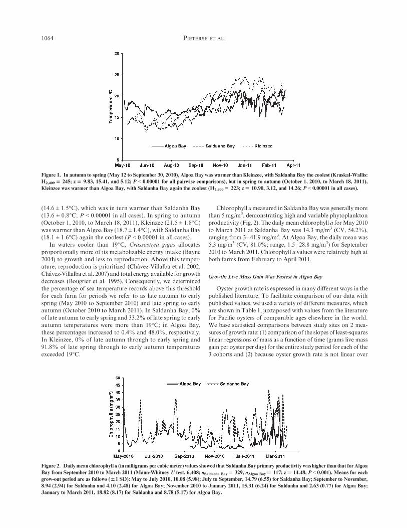
differences among farms emerged seasonally: in autumn tospring (May 12 to September 30, 2010), Algoa Bay (mean ofdaily means, 16.7 ± 0.9�C (1 SD)) was warmer than Kleinzee
PACIFIC OYSTER GROWTH IN SOUTH AFRICA 1063
(14.6 ± 1.5�C), which was in turn warmer than Saldanha Bay(13.6 ± 0.8�C; P < 0.00001 in all cases). In spring to autumn(October 1, 2010, to March 18, 2011), Kleinzee (21.5 ± 1.8�C)was warmer than Algoa Bay (18.7 ± 1.4�C), with Saldanha Bay(18.1 ± 1.6�C) again the coolest (P < 0.00001 in all cases).
In waters cooler than 19�C, Crassostrea gigas allocates
proportionally more of its metabolizable energy intake (Bayne2004) to growth and less to reproduction. Above this temper-ature, reproduction is prioritized (Chavez-Villalba et al. 2002,Chavez-Villalba et al. 2007) and total energy available for growth
decreases (Bougrier et al. 1995). Consequently, we determinedthe percentage of sea temperature records above this thresholdfor each farm for periods we refer to as late autumn to early
spring (May 2010 to September 2010) and late spring to earlyautumn (October 2010 to March 2011). In Saldanha Bay, 0%of late autumn to early spring and 33.2% of late spring to early
autumn temperatures were more than 19�C; in Algoa Bay,these percentages increased to 0.4% and 48.0%, respectively.In Kleinzee, 0% of late autumn through to early spring and91.8% of late spring through to early autumn temperatures
exceeded 19�C.
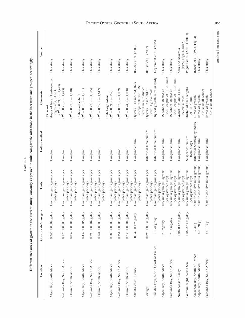
Chlorophyll ameasured in Saldanha Baywas generallymorethan 5 mg/m3, demonstrating high and variable phytoplanktonproductivity (Fig. 2). The daily mean chlorophyll a forMay 2010
to March 2011 at Saldanha Bay was 14.3 mg/m3 (CV, 54.2%),ranging from 3–41.9 mg/m3. At Algoa Bay, the daily mean was5.3 mg/m3 (CV, 81.0%; range, 1.5–28.8 mg/m3) for September
2010 toMarch 2011. Chlorophyll a values were relatively high atboth farms from February to April 2011.
Growth: Live Mass Gain Was Fastest in Algoa Bay
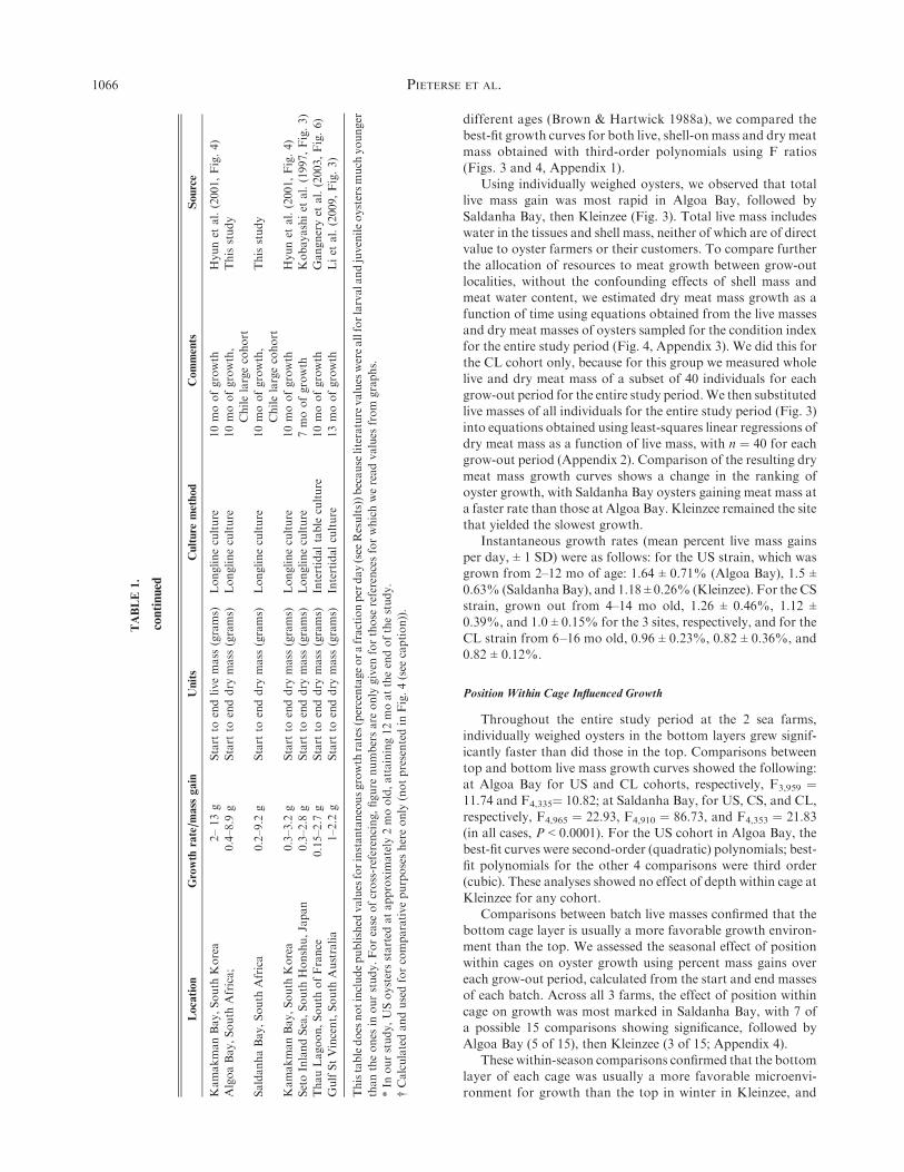
Oyster growth rate is expressed in many different ways in thepublished literature. To facilitate comparison of our data with
published values, we used a variety of different measures, whichare shown in Table 1, juxtaposed with values from the literaturefor Pacific oysters of comparable ages elsewhere in the world.
We base statistical comparisons between study sites on 2 mea-sures of growth rate: (1) comparison of the slopes of least-squareslinear regressions of mass as a function of time (grams live massgain per oyster per day) for the entire study period for each of the
3 cohorts and (2) because oyster growth rate is not linear over
Figure 2. Daily mean chlorophyll a (in milligrams per cubic meter) values showed that SaldanhaBay primary productivity was higher than that for Algoa
Bay from September 2010 to March 2011 (Mann-Whitney U test, 6,408; nSaldanha Bay$ 329, nAlgoa Bay$ 117; z$ 14.48; P < 0.001). Means for each
grow-out period are as follows (%1 SD): May to July 2010, 10.08 (5.98); July to September, 14.79 (6.55) for Saldanha Bay; September to November,
8.94 (2.94) for Saldanha and 4.10 (2.48) for Algoa Bay; November 2010 to January 2011, 15.31 (6.24) for Saldanha and 2.63 (0.77) for Algoa Bay;
January to March 2011, 18.82 (8.17) for Saldanha and 8.78 (5.17) for Algoa Bay.
Figure 1. In autumn to spring (May 12 to September 30, 2010), Algoa Bay was warmer than Kleinzee, with Saldanha Bay the coolest (Kruskal-Wallis:
H2,409$ 245; z$ 9.83, 15.41, and 5.12; P < 0.00001 for all pairwise comparisons), but in spring to autumn (October 1, 2010, to March 18, 2011),
Kleinzee was warmer than Algoa Bay, with Saldanha Bay again the coolest (H2,499$ 223; z$ 10.90, 3.12, and 14.26; P < 0.00001 in all cases).
PIETERSE ET AL.1064
TABLE1.
Differentmeasuresofgrowth
inthecurrentstudy,variouslyexpressed
inunitscomparablewiththose
intheliterature
andgrouped
accordingly.
Location
Growth
rate/m
ass
gain
Units
Culture
method
Comments
Source
UScohort
AlgoaBay,South
Africa
0.246±0.004g/day
Livemass
gain
(gramsper
oyster
per
day)
Longline
Slopes
oflinearleast-squares
regression,±1SD
(R2¼
0.69,n¼
1,473)
Thisstudy
SaldanhaBay,South
Africa
0.173±0.003g/day
Livemass
gain
(gramsper
oyster
per
day)
Longline
(R2¼
0.71,n¼
1,493)
Thisstudy
Kleinzee,South
Africa
0.037±0.001g/day
Livemass
gain
(gramsper
oyster
per
day)
Longline
(R2¼
0.27,n¼
1,810)
Thisstudy
Chilesm
allcohort
AlgoaBay,South
Africa
0.439±0.006g/day
Livemass
gain
(gramsper
oyster
per
day)
Longline
(R2¼
0.81,n¼
1,251)
Thisstudy
SaldanhaBay,South
Africa
0.298±0.004g/day
Livemass
gain
(gramsper
oyster
per
day)
Longline
(R2¼
0.77,n¼
1,385)
Thisstudy
Kleinzee,South
Africa
0.144±0.003g/day
Livemass
gain
(gramsper
oyster
per
day)
Longline
(R2¼
0.65,n¼
1,642)
Thisstudy
Chilelargecohort
AlgoaBay,South
Africa
0.580±0.007g/day
Livemass
gain
(gramsper
oyster
per
day)
Longline
(R2¼
0.89,n¼
857)
Thisstudy
SaldanhaBay,South
Africa
0.351±0.008g/day
Livemass
gain
(gramsper
oyster
per
day)
Longline
(R2¼
0.67,n¼
1,069)
Thisstudy
Kleinzee,South
Africa
0.233±0.004g/day
Livemass
gain
(gramsper
oyster
per
day)
Longline
(R2¼
0.74,n¼
1,068)
Thisstudy
Atlanticcoast,France
0.047–0.175g/day
Livemass
gain
(gramsper
oyster
per
day)
Longlineculture
Oysters3–10moold,thus
comparable
withUS
strain
inourstudy*
Boudry
etal.(2003)
Portugal
0.098±0.031g/day
Livemass
gain
(gramsper
oyster
per
day)
Intertidaltable
culture
Oysters;7moold
at
start,1glivemass
Batistaet
al.(2007)
Baiedes
Veys,NorthCoastofFrance
0.178g/day
Livemass
gain
(gramsper
oyster
per
day)
Intertidaltable
culture
Highestgrowth
ratesin
study
Degremontet
al.(2005)
AlgoaBay,South
Africa
23mg/day
Dry
mass
gain
(milligrams
per
oyster
per
day)
Longlineculture
UScohort,started
at
shelllengthsof10–20mm†
Thisstudy
SaldanhaBay,South
Africa
23.7
mg/day
Dry
mass
gain
(milligrams
per
oyster
per
day)
Longlineculture
UScohort,started
at
shelllengthsof10–20mm
Thisstudy
Northcoast
ofSicily
0.06–0.12mg/day
Dry
mass
gain
(milligrams
per
oyster
per
day)
Longlineculture
Grown7m
and13m
below
surface
Sara
andMazzola
(1997,Figs.4and5)
GermanBight,NorthSea
0.86–2.33mg/day
Dry
mass
gain
(milligrams
per
oyster
per
day)
Suspended
culture
from
buoys
Started
atshelllengths
of10–20mm
Pogodaet
al.(2011,Table
3)
ArcachonBay,South
ofFrance
3–40g
Start
toendlivemass
(grams)
IntertidalStanwaycylinders
13moofgrowth
Robertet
al.(1993,Fig.4)
AlgoaBay,South
Africa;
3.0–150g
Start
toendlivemass
(grams)
Longlineculture
10moofgrowth,
Chilesm
allcohort
Thisstudy
SaldanhaBay,South
Africa;
3.4–105g
Start
toendlivemass
(grams)
Longlineculture
10moofgrowth,
Chilesm
allcohort
Thisstudy
continued
onnextpage
PACIFIC OYSTER GROWTH IN SOUTH AFRICA 1065
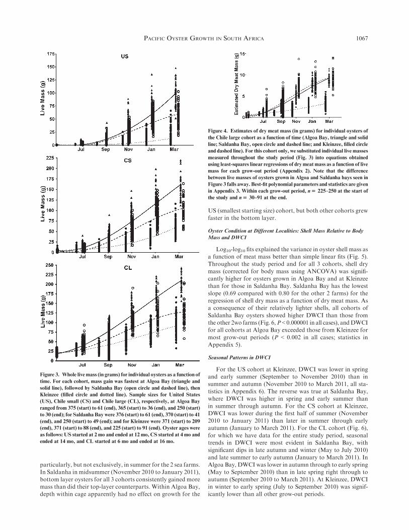
different ages (Brown & Hartwick 1988a), we compared thebest-fit growth curves for both live, shell-onmass and dry meat
mass obtained with third-order polynomials using F ratios(Figs. 3 and 4, Appendix 1).
Using individually weighed oysters, we observed that totallive mass gain was most rapid in Algoa Bay, followed by
Saldanha Bay, then Kleinzee (Fig. 3). Total live mass includeswater in the tissues and shell mass, neither of which are of directvalue to oyster farmers or their customers. To compare further
the allocation of resources to meat growth between grow-outlocalities, without the confounding effects of shell mass andmeat water content, we estimated dry meat mass growth as a
function of time using equations obtained from the live massesand dry meat masses of oysters sampled for the condition indexfor the entire study period (Fig. 4, Appendix 3). We did this forthe CL cohort only, because for this group we measured whole
live and dry meat mass of a subset of 40 individuals for eachgrow-out period for the entire study period.We then substitutedlive masses of all individuals for the entire study period (Fig. 3)
into equations obtained using least-squares linear regressions ofdry meat mass as a function of live mass, with n ¼ 40 for eachgrow-out period (Appendix 2). Comparison of the resulting dry
meat mass growth curves shows a change in the ranking ofoyster growth, with Saldanha Bay oysters gaining meat mass ata faster rate than those at Algoa Bay. Kleinzee remained the site
that yielded the slowest growth.Instantaneous growth rates (mean percent live mass gains
per day, ± 1 SD) were as follows: for the US strain, which wasgrown from 2–12 mo of age: 1.64 ± 0.71% (Algoa Bay), 1.5 ±0.63% (Saldanha Bay), and 1.18 ± 0.26% (Kleinzee). For the CSstrain, grown out from 4–14 mo old, 1.26 ± 0.46%, 1.12 ±0.39%, and 1.0 ± 0.15% for the 3 sites, respectively, and for the
CL strain from 6–16 mo old, 0.96 ± 0.23%, 0.82 ± 0.36%, and0.82 ± 0.12%.
Position Within Cage Influenced Growth
Throughout the entire study period at the 2 sea farms,individually weighed oysters in the bottom layers grew signif-
icantly faster than did those in the top. Comparisons betweentop and bottom live mass growth curves showed the following:at Algoa Bay for US and CL cohorts, respectively, F3,959 ¼11.74 and F4,335¼ 10.82; at Saldanha Bay, for US, CS, and CL,respectively, F4,965 ¼ 22.93, F4,910 ¼ 86.73, and F4,353 ¼ 21.83(in all cases, P < 0.0001). For the US cohort in Algoa Bay, the
best-fit curves were second-order (quadratic) polynomials; best-fit polynomials for the other 4 comparisons were third order(cubic). These analyses showed no effect of depth within cage at
Kleinzee for any cohort.Comparisons between batch live masses confirmed that the
bottom cage layer is usually a more favorable growth environ-ment than the top. We assessed the seasonal effect of position
within cages on oyster growth using percent mass gains overeach grow-out period, calculated from the start and end massesof each batch. Across all 3 farms, the effect of position within
cage on growth was most marked in Saldanha Bay, with 7 ofa possible 15 comparisons showing significance, followed byAlgoa Bay (5 of 15), then Kleinzee (3 of 15; Appendix 4).
These within-season comparisons confirmed that the bottomlayer of each cage was usually a more favorable microenvi-ronment for growth than the top in winter in Kleinzee, and
TABLE1.
continued
Location
Growth
rate/m
ass
gain
Units
Culture
method
Comments
Source
KamakmanBay,South
Korea
2–13g
Start
toendlivemass
(grams)
Longlineculture
10moofgrowth
Hyunet
al.(2001,Fig.4)
AlgoaBay,South
Africa;
0.4–8.9
gStart
toenddry
mass
(grams)
Longlineculture
10moofgrowth,
Chilelargecohort
Thisstudy
SaldanhaBay,South
Africa
0.2–9.2
gStart
toenddry
mass
(grams)
Longlineculture
10moofgrowth,
Chilelargecohort
Thisstudy
KamakmanBay,South
Korea
0.3–3.2
gStart
toenddry
mass
(grams)
Longlineculture
10moofgrowth
Hyunet
al.(2001,Fig.4)
SetoInlandSea,South
Honshu,Japan
0.3–2.8
gStart
toenddry
mass
(grams)
Longlineculture
7moofgrowth
Kobayashiet
al.(1997,Fig.3)
ThauLagoon,South
ofFrance
0.15–2.7
gStart
toenddry
mass
(grams)
Intertidaltable
culture
10moofgrowth
Gangneryet
al.(2003,Fig.6)
GulfStVincent,South
Australia
1–2.2
gStart
toenddry
mass
(grams)
Intertidalculture
13moofgrowth
Liet
al.(2009,Fig.3)
Thistabledoes
notincludepublished
values
forinstantaneousgrowth
rates(percentageorafractionper
day(see
Results))because
literature
values
wereallforlarvalandjuvenileoystersmuch
younger
thantheones
inourstudy.Forease
ofcross-referencing,figure
numbersare
only
given
forthose
referencesforwhichwereadvalues
from
graphs.
*In
ourstudy,USoystersstarted
atapproxim
ately
2moold,attaining12moattheendofthestudy.
†Calculatedandusedforcomparativepurposeshereonly
(notpresentedin
Fig.4(see
caption)).
PIETERSE ET AL.1066
particularly, but not exclusively, in summer for the 2 sea farms.In Saldanha in midsummer (November 2010 to January 2011),
bottom layer oysters for all 3 cohorts consistently gained moremass than did their top-layer counterparts. Within Algoa Bay,depth within cage apparently had no effect on growth for the
US (smallest starting size) cohort, but both other cohorts grewfaster in the bottom layer.
Oyster Condition at Different Localities: Shell Mass Relative to Body
Mass and DWCI
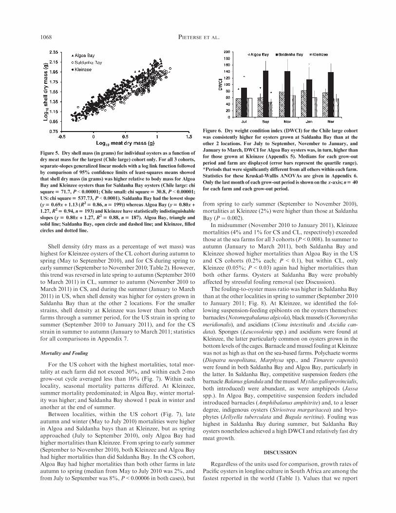
Log10-log10 fits explained the variance in oyster shell mass asa function of meat mass better than simple linear fits (Fig. 5).Throughout the study period and for all 3 cohorts, shell dry
mass (corrected for body mass using ANCOVA) was signifi-cantly higher for oysters grown in Algoa Bay and at Kleinzeethan for those in Saldanha Bay. Saldanha Bay has the lowest
slope (0.69 compared with 0.80 for the other 2 farms) for theregression of shell dry mass as a function of dry meat mass. Asa consequence of their relatively lighter shells, all cohorts of
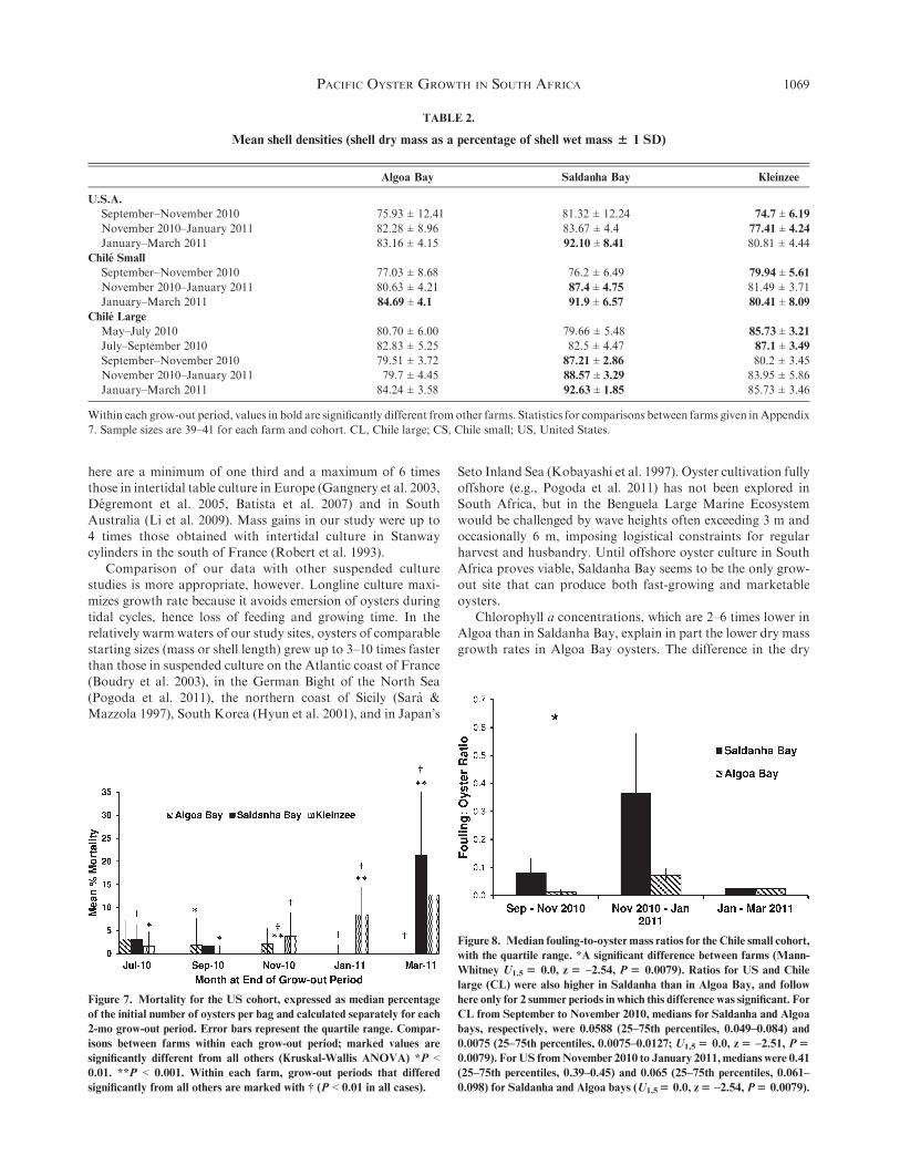
Saldanha Bay oysters showed higher DWCI than those fromthe other 2wo farms (Fig. 6,P < 0.000001 in all cases), andDWCIfor all cohorts at Algoa Bay exceeded those from Kleinzee for
most grow-out periods (P < 0.002 in all cases; statistics inAppendix 5).
Seasonal Patterns in DWCI
For the US cohort at Kleinzee, DWCI was lower in springand early summer (September to November 2010) than in
summer and autumn (November 2010 to March 2011, all sta-tistics in Appendix 6). The reverse was true at Saldanha Bay,where DWCI was higher in spring and early summer than
in summer through autumn. For the CS cohort at Kleinzee,DWCI was lower during the first half of summer (November2010 to January 2011) than later in summer through earlyautumn (January to March 2011). For the CL cohort (Fig. 6),
for which we have data for the entire study period, seasonaltrends in DWCI were most evident in Saldanha Bay, withsignificant dips in late autumn and winter (May to July 2010)
and late summer to early autumn (January to March 2011). InAlgoa Bay, DWCI was lower in autumn through to early spring(May to September 2010) than in late spring right through to
autumn (September 2010 to March 2011). At Kleinzee, DWCIin winter to early spring (July to September 2010) was signif-icantly lower than all other grow-out periods.
Figure 4. Estimates of dry meat mass (in grams) for individual oysters of
the Chile large cohort as a function of time (Algoa Bay, triangle and solid
line; Saldanha Bay, open circle and dashed line; and Kleinzee, filled circle
and dashed line). For this cohort only, we substituted individual live masses
measured throughout the study period (Fig. 3) into equations obtained
using least-squares linear regressions of dry meat mass as a function of live
mass for each grow-out period (Appendix 2). Note that the difference
between live masses of oysters grown in Algoa and Saldanha bays seen in
Figure 3 falls away. Best-fit polynomial parameters and statistics are given
in Appendix 3. Within each grow-out period, n$ 225–250 at the start of
the study and n$ 30–91 at the end.
Figure 3. Whole live mass (in grams) for individual oysters as a function of
time. For each cohort, mass gain was fastest at Algoa Bay (triangle and
solid line), followed by Saldanha Bay (open circle and dashed line), then
Kleinzee (filled circle and dotted line). Sample sizes for United States
(US), Chile small (CS) and Chile large (CL), respectively, at Algoa Bay
ranged from 375 (start) to 61 (end), 365 (start) to 36 (end), and 250 (start)
to 30 (end); for Saldanha Bay were 376 (start) to 61 (end), 370 (start) to 41
(end), and 250 (start) to 49 (end); and for Kleinzee were 371 (start) to 209
(end), 371 (start) to 88 (end), and 225 (start) to 91 (end). Oyster ages were
as follows: US started at 2 mo and ended at 12 mo, CS started at 4 mo and
ended at 14 mo, and CL started at 6 mo and ended at 16 mo.
PACIFIC OYSTER GROWTH IN SOUTH AFRICA 1067
Shell density (dry mass as a percentage of wet mass) was
highest for Kleinzee oysters of the CL cohort during autumn tospring (May to September 2010), and for CS during spring toearly summer (September toNovember 2010; Table 2). However,
this trend was reversed in late spring to autumn (September 2010to March 2011) in CL, summer to autumn (November 2010 toMarch 2011) in CS, and during the summer (January to March
2011) in US, when shell density was higher for oysters grown inSaldanha Bay than at the other 2 locations. For the smallerstrains, shell density at Kleinzee was lower than both other
farms through a summer period, for the US strain in spring tosummer (September 2010 to January 2011), and for the CSstrain in summer to autumn (January toMarch 2011; statisticsfor all comparisons in Appendix 7.
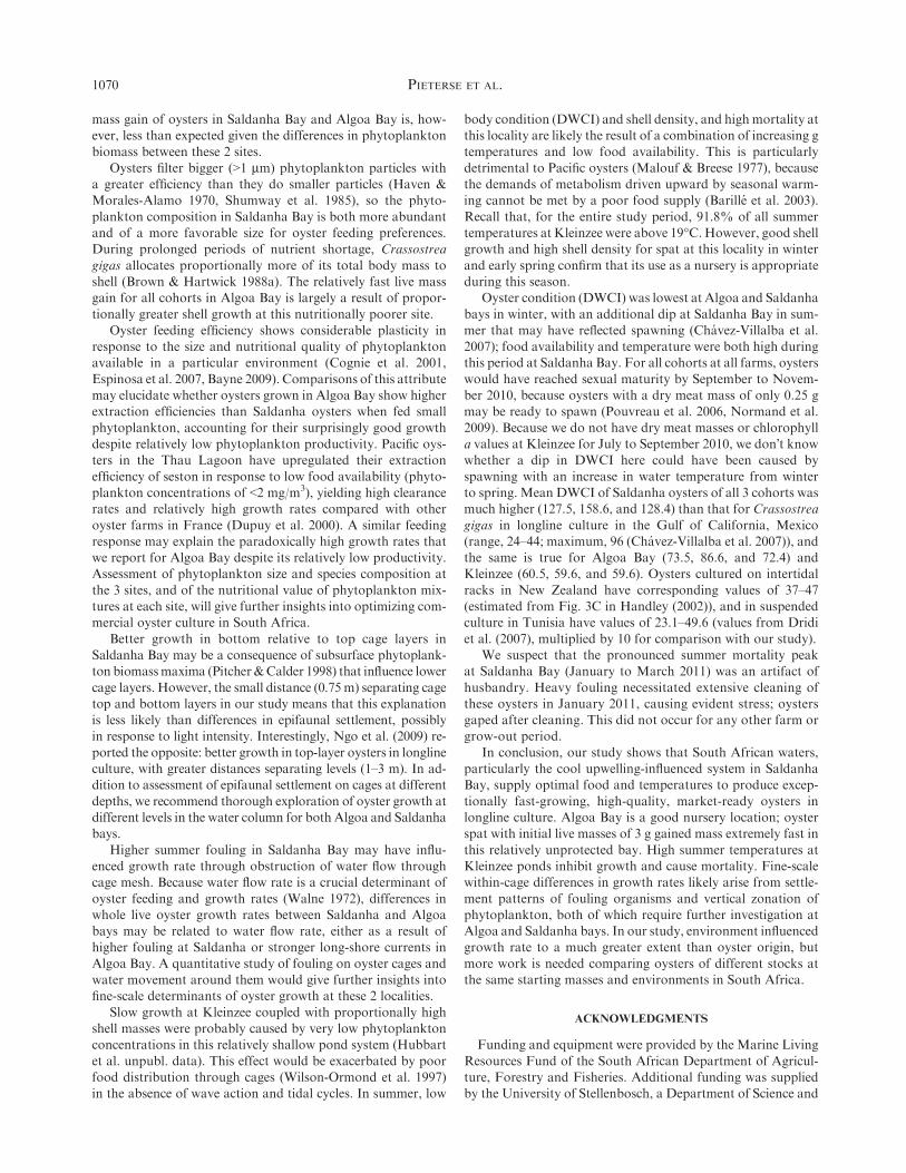
Mortality and Fouling
For the US cohort with the highest mortalities, total mor-
tality at each farm did not exceed 30%, and within each 2-mogrow-out cycle averaged less than 10% (Fig. 7). Within eachlocality, seasonal mortality patterns differed. At Kleinzee,
summer mortality predominated; in Algoa Bay, winter mortal-ity was higher; and Saldanha Bay showed 1 peak in winter andanother at the end of summer.
Between localities, within the US cohort (Fig. 7), late
autumn and winter (May to July 2010) mortalities were higherin Algoa and Saldanha bays than at Kleinzee, but as springapproached (July to September 2010), only Algoa Bay had
higher mortalities than Kleinzee. From spring to early summer(September to November 2010), both Kleinzee and Algoa Bayhad higher mortalities than did Saldanha Bay. In the CS cohort,
Algoa Bay had higher mortalities than both other farms in lateautumn to spring (median from May to July 2010 was 2%, andfrom July to September was 8%, P < 0.00006 in both cases), but
from spring to early summer (September to November 2010),mortalities at Kleinzee (2%) were higher than those at SaldanhaBay (P ¼ 0.002).
In midsummer (November 2010 to January 2011), Kleinzeemortalities (4% and 1% for CS and CL, respectively) exceededthose at the sea farms for all 3 cohorts (P < 0.008). In summer toautumn (January to March 2011), both Saldanha Bay and
Kleinzee showed higher mortalities than Algoa Bay in the USand CS cohorts (0.2% each; P < 0.1), but within CL, onlyKleinzee (0.05%; P < 0.03) again had higher mortalities than
both other farms. Oysters at Saldanha Bay were probablyaffected by stressful fouling removal (see Discussion).
The fouling-to-oyster mass ratio was higher in Saldanha Bay
than at the other localities in spring to summer (September 2010to January 2011; Fig. 8). At Kleinzee, we identified the fol-lowing suspension-feeding epibionts on the oysters themselves:
barnacles (Notomegabalanus algicola), blackmussels (Choromytilusmeridionalis), and ascidians (Ciona intestinalis and Ascidia can-data). Sponges (Leucosolenia spp.) and ascidians were found atKleinzee, the latter particularly common on oysters grown in the
bottom levels of the cages. Barnacle andmussel fouling atKleinzeewas not as high as that on the sea-based farms. Polychaete worms(Diopatra neopolitana, Marphysa spp., and Timarete capensis)
were found in both Saldanha Bay and Algoa Bay, particularly inthe latter. In Saldanha Bay, competitive suspension feeders (thebarnacleBalanus glandula and themusselMytilus galloprovincialis,
both introduced) were abundant, as were amphipods (Jassaspp.). In Algoa Bay, competitive suspension feeders includedintroduced barnacles (Amphibalanus amphitrite) and, to a lesserdegree, indigenous oysters (Striostrea margaritacea) and bryo-
phytes (Jellyella tuberculata and Bugula neritina). Fouling washighest in Saldanha Bay during summer, but Saldanha Bayoysters nonetheless achieved a highDWCI and relatively fast dry
meat growth.
DISCUSSION
Regardless of the units used for comparison, growth rates ofPacific oysters in longline culture in South Africa are among thefastest reported in the world (Table 1). Values that we report
Figure 6. Dry weight condition index (DWCI) for the Chile large cohort
was consistently higher for oysters grown at Saldanha Bay than at the
other 2 locations. For July to September, November to January, and
January toMarch, DWCI for Algoa Bay oysters was, in turn, higher than
for those grown at Kleinzee (Appendix 5). Medians for each grow-out
period and farm are displayed (error bars represent the quartile range).
*Periods that were significantly different from all others within each farm.
Statistics for these Kruskal-Wallis ANOVAs are given in Appendix 6.
Only the last month of each grow-out period is shown on the x-axis; n$ 40
for each farm and each grow-out period.
Figure 5. Dry shell mass (in grams) for individual oysters as a function of
dry meat mass for the largest (Chile large) cohort only. For all 3 cohorts,
separate-slopes generalized linear models with a log link function followed
by comparison of 95% confidence limits of least-squares means showed
that shell dry mass (in grams) was higher relative to body mass for Algoa
Bay and Kleinzee oysters than for Saldanha Bay oysters (Chile large: chi
square$ 71.7, P < 0.00001; Chile small: chi square$ 30.8, P < 0.00001;
US: chi square$ 537.73, P < 0.0001). Saldanha Bay had the lowest slope
1.27,R2$ 0.94, n$ 193) and Kleinzee have statistically indistinguishable
slopes (y$ 0.80x + 1.27, R2$ 0.88, n$ 187). Algoa Bay, triangle and
solid line; Saldanha Bay, open circle and dashed line; and Kleinzee, filled
circles and dotted line.
PIETERSE ET AL.1068
here are a minimum of one third and a maximum of 6 timesthose in intertidal table culture in Europe (Gangnery et al. 2003,Degremont et al. 2005, Batista et al. 2007) and in South
Australia (Li et al. 2009). Mass gains in our study were up to4 times those obtained with intertidal culture in Stanwaycylinders in the south of France (Robert et al. 1993).
Comparison of our data with other suspended culturestudies is more appropriate, however. Longline culture maxi-mizes growth rate because it avoids emersion of oysters during
tidal cycles, hence loss of feeding and growing time. In therelatively warm waters of our study sites, oysters of comparablestarting sizes (mass or shell length) grew up to 3–10 times fasterthan those in suspended culture on the Atlantic coast of France
(Boudry et al. 2003), in the German Bight of the North Sea(Pogoda et al. 2011), the northern coast of Sicily (Sara &Mazzola 1997), South Korea (Hyun et al. 2001), and in Japan�s
Seto Inland Sea (Kobayashi et al. 1997). Oyster cultivation fullyoffshore (e.g., Pogoda et al. 2011) has not been explored inSouth Africa, but in the Benguela Large Marine Ecosystem
would be challenged by wave heights often exceeding 3 m andoccasionally 6 m, imposing logistical constraints for regularharvest and husbandry. Until offshore oyster culture in South
Africa proves viable, Saldanha Bay seems to be the only grow-out site that can produce both fast-growing and marketableoysters.
Chlorophyll a concentrations, which are 2–6 times lower inAlgoa than in Saldanha Bay, explain in part the lower dry massgrowth rates in Algoa Bay oysters. The difference in the dry
Figure 8. Median fouling-to-oyster mass ratios for the Chile small cohort,
with the quartile range. *A significant difference between farms (Mann-
Whitney U1,5$ 0.0, z$ –2.54, P$ 0.0079). Ratios for US and Chile
large (CL) were also higher in Saldanha than in Algoa Bay, and follow
here only for 2 summer periods in which this difference was significant. For
CL from September to November 2010, medians for Saldanha and Algoa
bays, respectively, were 0.0588 (25–75th percentiles, 0.049–0.084) and
Within each grow-out period, values in bold are significantly different fromother farms. Statistics for comparisons between farms given inAppendix
7. Sample sizes are 39–41 for each farm and cohort. CL, Chile large; CS, Chile small; US, United States.
PACIFIC OYSTER GROWTH IN SOUTH AFRICA 1069
mass gain of oysters in Saldanha Bay and Algoa Bay is, how-ever, less than expected given the differences in phytoplankton
biomass between these 2 sites.Oysters filter bigger (>1 mm) phytoplankton particles with
a greater efficiency than they do smaller particles (Haven &Morales-Alamo 1970, Shumway et al. 1985), so the phyto-
plankton composition in Saldanha Bay is both more abundantand of a more favorable size for oyster feeding preferences.During prolonged periods of nutrient shortage, Crassostrea
gigas allocates proportionally more of its total body mass toshell (Brown & Hartwick 1988a). The relatively fast live massgain for all cohorts in Algoa Bay is largely a result of propor-
tionally greater shell growth at this nutritionally poorer site.Oyster feeding efficiency shows considerable plasticity in
response to the size and nutritional quality of phytoplanktonavailable in a particular environment (Cognie et al. 2001,
Espinosa et al. 2007, Bayne 2009). Comparisons of this attributemay elucidate whether oysters grown in Algoa Bay show higherextraction efficiencies than Saldanha oysters when fed small
phytoplankton, accounting for their surprisingly good growthdespite relatively low phytoplankton productivity. Pacific oys-ters in the Thau Lagoon have upregulated their extraction
efficiency of seston in response to low food availability (phyto-plankton concentrations of <2 mg/m3), yielding high clearancerates and relatively high growth rates compared with other
oyster farms in France (Dupuy et al. 2000). A similar feedingresponse may explain the paradoxically high growth rates thatwe report for Algoa Bay despite its relatively low productivity.Assessment of phytoplankton size and species composition at
the 3 sites, and of the nutritional value of phytoplankton mix-tures at each site, will give further insights into optimizing com-mercial oyster culture in South Africa.
Better growth in bottom relative to top cage layers inSaldanha Bay may be a consequence of subsurface phytoplank-ton biomassmaxima (Pitcher&Calder 1998) that influence lower
cage layers. However, the small distance (0.75 m) separating cagetop and bottom layers in our study means that this explanationis less likely than differences in epifaunal settlement, possiblyin response to light intensity. Interestingly, Ngo et al. (2009) re-
ported the opposite: better growth in top-layer oysters in longlineculture, with greater distances separating levels (1–3 m). In ad-dition to assessment of epifaunal settlement on cages at different
depths, we recommend thorough exploration of oyster growth atdifferent levels in the water column for both Algoa and Saldanhabays.
Higher summer fouling in Saldanha Bay may have influ-enced growth rate through obstruction of water flow throughcage mesh. Because water flow rate is a crucial determinant of
oyster feeding and growth rates (Walne 1972), differences inwhole live oyster growth rates between Saldanha and Algoabays may be related to water flow rate, either as a result ofhigher fouling at Saldanha or stronger long-shore currents in
Algoa Bay. A quantitative study of fouling on oyster cages andwater movement around them would give further insights intofine-scale determinants of oyster growth at these 2 localities.
Slow growth at Kleinzee coupled with proportionally highshell masses were probably caused by very low phytoplanktonconcentrations in this relatively shallow pond system (Hubbart
et al. unpubl. data). This effect would be exacerbated by poorfood distribution through cages (Wilson-Ormond et al. 1997)in the absence of wave action and tidal cycles. In summer, low
body condition (DWCI) and shell density, and high mortality atthis locality are likely the result of a combination of increasing g
temperatures and low food availability. This is particularlydetrimental to Pacific oysters (Malouf & Breese 1977), becausethe demands of metabolism driven upward by seasonal warm-ing cannot be met by a poor food supply (Barille et al. 2003).
Recall that, for the entire study period, 91.8% of all summertemperatures at Kleinzee were above 19�C.However, good shellgrowth and high shell density for spat at this locality in winter
and early spring confirm that its use as a nursery is appropriateduring this season.
Oyster condition (DWCI) was lowest at Algoa and Saldanha
bays in winter, with an additional dip at Saldanha Bay in sum-mer that may have reflected spawning (Chavez-Villalba et al.2007); food availability and temperature were both high duringthis period at Saldanha Bay. For all cohorts at all farms, oysters
would have reached sexual maturity by September to Novem-ber 2010, because oysters with a dry meat mass of only 0.25 gmay be ready to spawn (Pouvreau et al. 2006, Normand et al.
2009). Because we do not have dry meat masses or chlorophylla values at Kleinzee for July to September 2010, we don�t knowwhether a dip in DWCI here could have been caused by
spawning with an increase in water temperature from winterto spring. Mean DWCI of Saldanha oysters of all 3 cohorts wasmuch higher (127.5, 158.6, and 128.4) than that for Crassostrea
gigas in longline culture in the Gulf of California, Mexico(range, 24–44; maximum, 96 (Chavez-Villalba et al. 2007)), andthe same is true for Algoa Bay (73.5, 86.6, and 72.4) andKleinzee (60.5, 59.6, and 59.6). Oysters cultured on intertidal
racks in New Zealand have corresponding values of 37–47(estimated from Fig. 3C in Handley (2002)), and in suspendedculture in Tunisia have values of 23.1–49.6 (values from Dridi
et al. (2007), multiplied by 10 for comparison with our study).We suspect that the pronounced summer mortality peak
at Saldanha Bay (January to March 2011) was an artifact of
husbandry. Heavy fouling necessitated extensive cleaning ofthese oysters in January 2011, causing evident stress; oystersgaped after cleaning. This did not occur for any other farm orgrow-out period.
In conclusion, our study shows that South African waters,particularly the cool upwelling-influenced system in SaldanhaBay, supply optimal food and temperatures to produce excep-
tionally fast-growing, high-quality, market-ready oysters inlongline culture. Algoa Bay is a good nursery location; oysterspat with initial live masses of 3 g gained mass extremely fast in
this relatively unprotected bay. High summer temperatures atKleinzee ponds inhibit growth and cause mortality. Fine-scalewithin-cage differences in growth rates likely arise from settle-
ment patterns of fouling organisms and vertical zonation ofphytoplankton, both of which require further investigation atAlgoa and Saldanha bays. In our study, environment influencedgrowth rate to a much greater extent than oyster origin, but
more work is needed comparing oysters of different stocks atthe same starting masses and environments in South Africa.
ACKNOWLEDGMENTS
Funding and equipment were provided by the Marine Living
Resources Fund of the South African Department of Agricul-ture, Forestry and Fisheries. Additional funding was suppliedby the University of Stellenbosch, a Department of Science and
PIETERSE ET AL.1070
Technology–National Research Foundation internship toA. P., and the Institute for Animal Production at the Western
Cape Provincial Department of Agriculture at Elsenburg. In par-ticular, we thank our industry partners Simon Daniel, JosephDayimani, Alister Joshua, and Quiryn Snethlage for invaluable
advice and logistical and technical support, and Antonio Toninfor extensive help with study design and equipment loans.
Bernie Hubbart�s indispensable help in the field and laboratoryis deeply appreciated. This study is dedicated to the memory ofRoger Denton, a unique and gentle soul.
LITERATURE CITED
Agius, C., V. Jaccarini & D. A. Ritz. 1978. Growth trials of Crassostrea
gigas and Ostrea edulis in inshore waters of Malta (Central
Mediterranean). Aquaculture 15:195–218.
Barille, L., J. Haure, E. Pales-Espinosa & M. Morancxais. 2003.
Finding new diatoms for intensive rearing of the Pacific oyster
(Crassostrea gigas): energy budget as a selective tool. Aquaculture
217:501–514.
Barille, L., J. Prou, M. Heral & D. Razet. 1997. Effects of high natural
seston concentrations on the feeding, selection, and absorption of
the oyster Crassostrea gigas (Thunberg). J. Exp. Mar. Biol. Ecol.
212:149–172.
Batista, F. M., A. Leitao, V. G. Fonseca, R. Ben-Hamadou, F. Ruano,
M. A. Henriques, H. Guedes-Pinto & P. Boudry. 2007. Individual
relationship between aneuploidy of gill cells and growth rate in the
cupped oysters Crassostrea angulata, C. gigas and their reciprocal
hybrids. J. Exp. Mar. Biol. Ecol. 352:226–233.
Bayne, B. L. 2004. Phenotypic flexibility and physiological tradeoffs in
the feeding and growth of marine bivalve molluscs. Integr. Comp.
Biol. 44:425–432.
Bayne, B. L. 2009. Carbon and nitrogen relationships in the feeding and
growth of the Pacific oyster, Crassostrea gigas (Thunberg). J. Exp.
Mar. Biol. Ecol. 374:19–30.
Bayne, B. L., D. Hedgecock, D. McGoldrick & R. Rees. 1999. Feeding
behaviour andmetabolic efficiency contribute to growth heterosis in
Pacific oysters [Crassostrea gigas (Thunberg)]. J. Exp. Mar. Biol.
Ecol. 233:115–130.
Boudry, P., B. Collet, H. McCombie, B. Ernandez, B. Morand, S.
Heurtebise & A. Gerard. 2003. Individual growth variation and its
relationship with survival in juvenile Pacific oysters, Crassostrea
gigas (Thunberg). Aquacult. Int. 11:429–448.
Bougrier, S., P. Geairon, J. M. Deslous-Paoli, C. Bacher & G.
Jonquieres. 1995. Allometric relationships and effects of tempera-
ture on clearance and oxygen consumption rates of Crassostrea
gigas (Thunberg). Aquaculture 134:143–154.
Branch,G.M., C. L.Griffiths,M. L. Branch&L. E. Beckley. 2010. Two
oceans: a guide to the marine life of southern Africa, revised edition.
Cape Town: Struik Nature. 455 pp.
Brown, J. R. 1988. Multivariate analyses of the role of environmental
factors in seasonal and site-related growth variation in the Pacific
oyster Crassostrea gigas. Mar. Ecol. Prog. Ser. 45:225–236.
Brown, J. R. & E. B. Hartwick. 1988a. Influences of temperature,
salinity and available food upon suspended culture of the Pacific
oyster, Crassostrea gigas: absolute and allometric growth. Aquacul-
ture 70:231–251.
Brown, J. R. & E. B. Hartwick. 1988b. Influences of temperature,
salinity and available food upon suspended culture of the Pacific
oyster, Crassostrea gigas: II. condition index and survival. Aqua-
culture 70:253–267.
Chavez-Villalba, J., J. Pommier, J. Andriamiseza, S. Pouvreau, J. Barret,
J.- C. Cochard&M. Le Pennec. 2002. Broodstock conditioning of the
oyster Crassostrea gigas: origin and temperature effect. Aquaculture
214:115–130.
Chavez-Villalba, J., R. Villelas-Avil & C. Caceres-Martınez. 2007. Re-
production, condition and mortality of the Pacific oyster Crassostrea
gigas (Thunberg) in Sonora, Mexico. Aquacult. Res. 38:268–278.
Cognie, B., L. Barille & Y. Rince. 2001. Selective feeding of the oyster
Crassostrea gigas fed on a natural microphytobenthos assemblage.
Estuaries 24:126–131.
Crosby, M. P. & L. D. Gale. 1990. A review and evaluation of bivalve
condition index methodologies with a suggested standard method.
J. Shellfish Res. 9:233–237.
David, E., P. Boudry, L.Degremont, A. Tanguy,N.Quere, J. F. Samain
&D.Moraga. 2007. Genetic polymorphism of glutamine synthetase
and delta-9 desaturase in families of Pacific oyster Crassostrea gigas
and susceptibility to summer mortality. J. Exp. Mar. Biol. Ecol.
349:272–283.
Degremont, L., E. Bedier, P. Soletchnik, M. Ropert, A. Huvete, J.
Moale, J.- F. Samaine & P. Boudry. 2005. Relative importance of
family, site, and field placement timing on survival, growth, and
yield of hatchery-produced Pacific oyster spat (Crassostrea gigas).
Aquaculture 249:213–229.
Dridi, S., M. S. Romdhanes & M. Elcafsi. 2007. Seasonal variation
in weight and biochemical composition of the Pacific oyster
Crassostrea gigas in relation to the gametogenic cycle and
environmental conditions of the Bizert Lagoon, Tunisia. Aquaculture
263:238–248.
Dupuy, C., A. Vaquer, T. Lam-Hoai, C. Rougier, N. Mazouni, J.
Lautier, Y. Collos & S. Le Gall. 2000. Feeding rate of the
oyster Crassostrea gigas in a natural planktonic community
of the Mediterranean Thau Lagoon. Mar. Ecol. Prog. Ser. 205:
171–184.
Espinosa, E. P., L. Barille & B. Allam. 2007. Use of encapsulated live
microalgae to investigate pre-ingestive selection in the oyster
Crassostrea gigas. J. Exp. Mar. Biol. Ecol. 343:118–126.
Evans, S. & C. Langdon. 2006. Effects of genotype 3 environment
interactions on the selection of broadly adapted Pacific oysters
(Crassostrea gigas). Aquaculture 261:522–534.
Flores-Vergara, C., B. Cordero-Esquivel, A. N. Ceron-Ortiz & B. O.
Arredondo-Vega. 2004. Combined effects of temperature and diet
on growth and biochemical composition of the Pacific oyster C.
The dry weight condition index was consistently higher at Saldanha Bay than at the other 2 environments and, likewise, higher at Algoa Bay than
at Kleinzee. Statistics are for Kruskal-Wallis ANOVAs, followed by z values for post hoc pairwise tests for which P < 0.001 unless otherwise stated;
n ¼ 39–41 oysters for each cohort at each locality. NS, not significant.
PACIFIC OYSTER GROWTH IN SOUTH AFRICA 1075
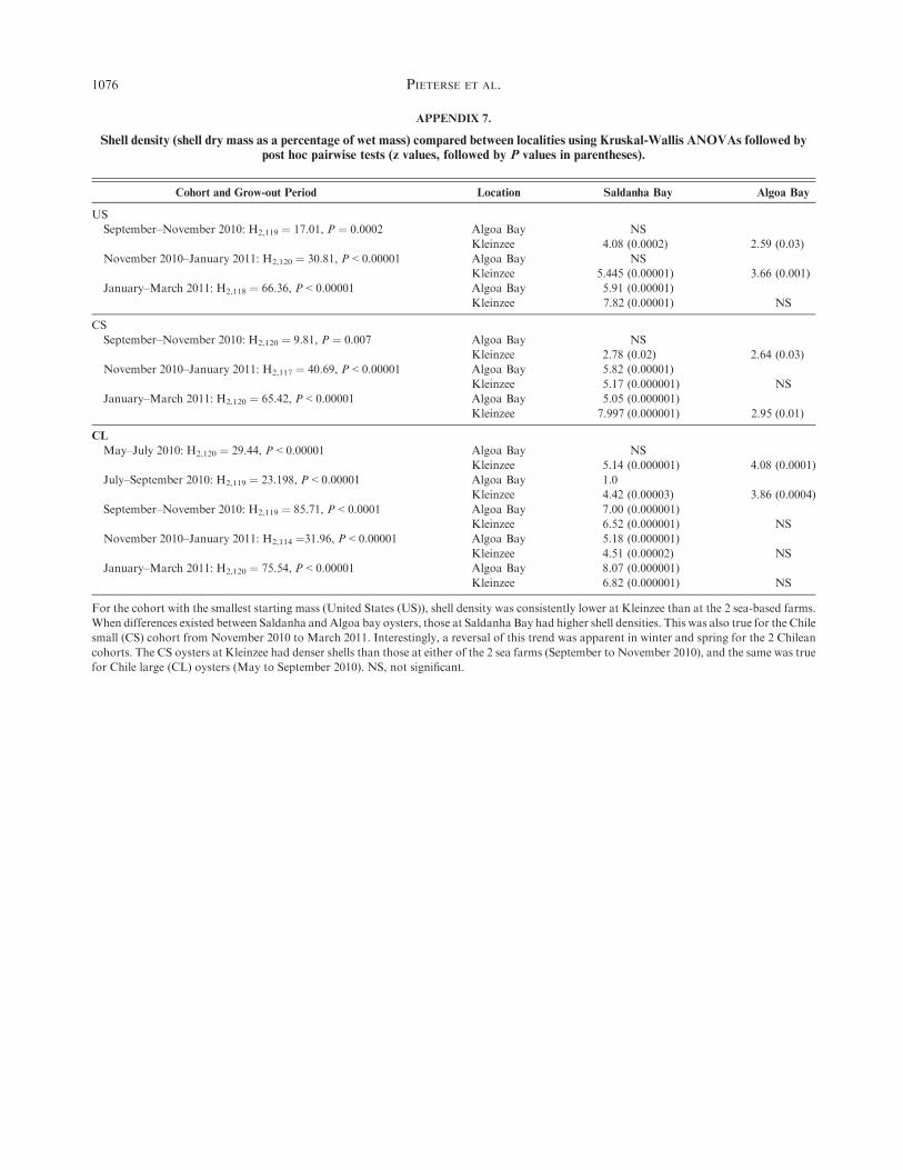
APPENDIX 7.
Shell density (shell dry mass as a percentage of wet mass) compared between localities using Kruskal-Wallis ANOVAs followed bypost hoc pairwise tests (z values, followed by P values in parentheses).
Cohort and Grow-out Period Location Saldanha Bay Algoa Bay
US
September–November 2010: H2,119 ¼ 17.01, P ¼ 0.0002 Algoa Bay NS
Kleinzee 4.08 (0.0002) 2.59 (0.03)
November 2010–January 2011: H2,120 ¼ 30.81, P < 0.00001 Algoa Bay NS
Kleinzee 5.445 (0.00001) 3.66 (0.001)
January–March 2011: H2,118 ¼ 66.36, P < 0.00001 Algoa Bay 5.91 (0.00001)
Kleinzee 7.82 (0.00001) NS
CS
September–November 2010: H2,120 ¼ 9.81, P ¼ 0.007 Algoa Bay NS
Kleinzee 2.78 (0.02) 2.64 (0.03)
November 2010–January 2011: H2,117 ¼ 40.69, P < 0.00001 Algoa Bay 5.82 (0.00001)
Kleinzee 5.17 (0.000001) NS
January–March 2011: H2,120 ¼ 65.42, P < 0.00001 Algoa Bay 5.05 (0.000001)
Kleinzee 7.997 (0.000001) 2.95 (0.01)
CL
May–July 2010: H2,120 ¼ 29.44, P < 0.00001 Algoa Bay NS
Kleinzee 5.14 (0.000001) 4.08 (0.0001)
July–September 2010: H2,119 ¼ 23.198, P < 0.00001 Algoa Bay 1.0
Kleinzee 4.42 (0.00003) 3.86 (0.0004)
September–November 2010: H2,119 ¼ 85.71, P < 0.0001 Algoa Bay 7.00 (0.000001)
Kleinzee 6.52 (0.000001) NS
November 2010–January 2011: H2,114 ¼31.96, P < 0.00001 Algoa Bay 5.18 (0.000001)
Kleinzee 4.51 (0.00002) NS
January–March 2011: H2,120 ¼ 75.54, P < 0.00001 Algoa Bay 8.07 (0.000001)
Kleinzee 6.82 (0.000001) NS
For the cohort with the smallest starting mass (United States (US)), shell density was consistently lower at Kleinzee than at the 2 sea-based farms.
When differences existed between Saldanha andAlgoa bay oysters, those at Saldanha Bay had higher shell densities. This was also true for the Chile
small (CS) cohort from November 2010 to March 2011. Interestingly, a reversal of this trend was apparent in winter and spring for the 2 Chilean
cohorts. The CS oysters at Kleinzee had denser shells than those at either of the 2 sea farms (September to November 2010), and the same was true
for Chile large (CL) oysters (May to September 2010). NS, not significant.