Growth and Structural Reforms: A New Assessment

Lone Christiansen, Martin Schindler,

and Thierry Tressel

WP/09/284

© 2009 International Monetary Fund WP/09/284 IMF Working Paper Research Department

Growth and Structural Reforms: A New Assessment*

Prepared by Lone Christiansen, Martin Schindler, and Thierry Tressel

Authorized for distribution by Gian Maria Milesi-Ferretti

December 2009

Abstract

This Working Paper should not be reported as representing the views of the IMF. The views expressed in this Working Paper are those of the author(s) and do not necessarily represent those of the IMF or IMF policy. Working Papers describe research in progress by the author(s) and are published to elicit comments and to further debate.

This paper presents a simultaneous assessment of the relationship between economic performanceand three groups of economic reforms: domestic finance, trade, and the capital account. Among these, domestic financial reforms, and trade reforms, are robustly associated with economic growth, butonly in middle-income countries. In contrast, we do not find any systematic positive relationshipbetween capital account liberalization and economic growth. Moreover, the effect of domestic financial reforms on economic growth in middle-income countries is explained by improvements in measured aggregate TFP growth, not by higher aggregate investment. We present evidence thatvariation in the quality of property rights helps explain the heterogeneity of the effectiveness offinancial and trade reforms in developing countries. The evidence suggests that sufficiently developedproperty rights are a precondition for reaping the benefits of economic reform. Our results are robust to endogeneity bias and a number of alternative specifications. JEL Classification Numbers: F3; G28; O24; O43

Keywords: Economic Growth; Liberalization; Domestic Finance; Trade: Capital Account

Author’s E-Mail Address: Lchristiansen@imf.org; MSchindler@imf.org; TTressel@imf.org

* We are indebted to the late Alessandro Prati for his encouragement and numerous suggestions on this paper. We are also grateful for comments and suggestions from Philippe Aghion, Raghu Rajan, Romain Wacziarg, participants at the ASSA 2009 Meetings and colleagues at the IMF, as well as to Dennis Quinn for providing access to his updated data set. Freddy Cama and Manzoor Gill provided able research assistance. The views expressed in this paper are those of the authors and not necessarily those of the IMF, its management or its executive board.

2

Contents Page

 I. Introduction ................................................................................................................................ 4  II. Related Literature ...................................................................................................................... 6  III. The Empirical Model ............................................................................................................... 9 

A. Standard Growth Regressions ............................................................................................... 9 B. Dynamic Effects of Reforms ............................................................................................... 10 

IV. Data Description .................................................................................................................... 11 

A. Data ..................................................................................................................................... 11 B. Descriptive Statistics ........................................................................................................... 13

V. Main Results ........................................................................................................................... 14 

A. Standard growth regressions ............................................................................................... 14 B. Dynamic Effects of Reforms ............................................................................................... 16

VI. Robustness Tests and endogeneity ........................................................................................ 18 

A. Robustness tests .................................................................................................................. 18 B. Endogeneity ......................................................................................................................... 19 

VII. Reform Sequencing and Economic Performance ................................................................. 21  VIII. Conclusion .......................................................................................................................... 23  References ................................................................................................................................... 25  Figures 1. ReformEpisodes…………………………………………………………………………….31

Tables 1. Country Sample……………………………………………………………………………..32 2. Summary Statistices………………………………………………………………………...33 3. Bivariate Correlations……………………………………………………………………….34 4. Standard Growth Regressions………………………………………………………………35 5. The Channels of the Effects of Liberalizations……………………………………………..36 6. System GMM Regressions………………………………………………………………….37 7. Baseline: Dynamic Effect of Reforms……………………………………………………...38 8. Channels Dynamic Effects of Reforms……………………………………………………..40 9. Robustness Tests Dynamic Effect of Reforms……………………………………………...42 10. Dynamic Effect of Reforms on TFP and Investment Robustness…………………………..44

3

11. A. Instrumental Variables Regressions Second Stage………………………………………46 B. Instrumental Variable Regressions Frist Stage…………………………………………..48

12. Sequencing Economic and Political Reforms………………………………………………49 Appendix Table: 2 SLS Regressions……………………………………………………………51

4

I. INTRODUCTION

Over the past decades, the global economy has become increasingly liberalized in a number of

dimensions: domestic financial systems have deepened and become less regulated, trade regimes

have become more open, and capital accounts have become less restricted. The trend towards

less regulated markets has been observed in all regions and in most countries. But to what extent

have these liberalization efforts contributed to improved economic outcomes, as measured by

per-capita income levels and growth?

The recent experience highlights the importance of deepening our understanding of the benefits

of structural reforms. As discussions about financial (re)regulation of financial systems indicate,

the answer to the above question is, even at a theoretical level, not obvious: in the context of the

recent global financial crisis, there have been claims that some regulation (of the right sort) may

help rather than hinder growth and macroeconomic stability.

A large literature exists on the economic benefits of reforms, but with some exceptions, existing

studies have typically focused on individual reforms only, and have covered different country

samples and measures of reforms, making comparisons across studies and types of reforms

difficult. Moreover, empirical studies have often relied on de facto measures to proxy for

liberalization, such as financial development as a proxy for financial liberalization, and openness

to trade as a proxy for trade reforms. While de facto measures are likely to be useful indicators of

the success of reforms, they are outcome measures that are influenced by a variety of

macroeconomic conditions beyond the reform considered.

The main contribution of this paper is to test the joint growth effects of various types of de jure

reforms, and to do so within a unified empirical framework, thus allowing for better

comparability across reforms. To our knowledge, it is the first one that simultaneously considers

domestic financial reforms, trade reforms, and capital account reforms. The aim is to provide

answers to the following key questions: (i) what do growth regressions tell us on the joint effects

of these reforms on economic performance; (ii) are the effects of reforms persistent; (iii) is there

heterogeneity of the effects of reforms across countries (if yes, are the growth effects constrained

by political institutions?); and (iv) what are the main channels through which reforms affect

5

economic performance—do reforms affect economic performance by increasing aggregate

investment or by improving aggregate economic efficiency?

To answer these questions, we draw on a newly developed database of de jure indicators of

structural reform in the areas of finance, trade and the capital account. The new database has

several advantages with respect to previous studies. First, some indicators used in previous

research, especially regarding domestic finance and capital account, were sometimes crude,

binary indicators. In our analysis, we rely on more refined measures. Second, by providing a

wide country and year coverage across all three indicators, the new database allows for better

comparability of the effects of reforms in these different areas—previous research has typically

focused on only a small subset of these reform areas, making comparisons difficult to interpret.

Finally, we focus exclusively on de jure indicators, that is, those reflecting legal and policy

restrictions, rather than de facto measures which reflect outcomes, as done in much of the

existing literature. While there is significant value in analyzing the correlations between de facto

measures and economic outcomes, de jure indicators are the more appropriate measures from a

policy perspective, as they are under the policymaker’s (direct) control.

To give an overview of our results, we find that among the three groups of reforms, domestic

financial reforms, and to some extent trade reforms, are most robustly associated with economic

growth; in contrast, we do not find any systematic positive relationship between capital account

liberalization and economic growth. Moreover, the positive effects of financial and trade reforms

are almost exclusively driven by the group of middle-income countries, and the effect of

domestic financial reforms on economic growth in these countries is predominantly explained by

improvements in measured aggregate TFP growth, not by higher aggregate investment. Also, the

growth effects of domestic financial and trade reforms are somewhat persistent, raising growth at

a horizon of up to 6 years, but become insignificant at a longer horizon.

We also present some tentative evidence on the interactions of political institutions (the quality

of property rights) and economic reforms. In particular, the heterogeneity of the effectiveness of

financial and trade reforms in developing countries seems to be explained by a complementarity

between economic reforms and political reforms: financial and trade reforms are effective in

developing countries with good protection of property rights. This evidence suggests that

sufficiently developed property rights may be a precondition for reaping the growth benefits of

6

reforms, a finding that is consistent with part of the recent literature in this area. Our results are

robust to a variety of robustness tests and, in particular, to endogeneity bias.

The remainder of the paper proceeds as follows. Section II provides an overview of the related

literature; section III presents the empirical model; section IV describes the data; section V

presents the main results; section VI discusses robustness tests and addresses endogeneity issues;

section VII examines the interactions of economic and political reforms; and section VIII

concludes.

II. RELATED LITERATURE

This paper examines the effects of economic reforms, specifically domestic financial

development, trade openness and capital account openness, on economic growth, with a focus on

how reforms in different areas interact in their effects on growth. While the literature on reform

interactions and sequencing is relatively sparse, the literature on the effects of individual reforms

is large. In the following, we discuss a subset of this literature.2

Levine (1997, 2005) provides a survey of the large literature on the growth benefits of domestic

financial reform. Empirical applications in this literature typically employ de facto measures of

domestic financial development (or depth), such as the ratio of private domestic credit, M2, or

liquid liabilities to GDP. This literature broadly provides strong evidence that a higher initial

level of financial development is associated with higher subsequent rates of economic growth,

and economic efficiency improvements even after controlling for a wide variety of economic

factors (Beck et al., 2000a and 2000b, Aghion et al., 2005). Using de jure measures, Bekaert et

al. (2005) and Henry (2005) find that stock market liberalizations are positively correlated with

economic growth and investment. Furthermore, Rajan and Zingales (1998), Galindo et al.

(2005), Abiad et al. (2008), and Tressel (2008) provide evidence suggesting that a more

2 The literature review in this section is highly selective. For example, a broader empirical literature exists on the sequencing of product and labor market reforms in OECD countries (e.g., Fiori and others, 2007), and their effect on economic outcomes (Scarpetta and Tressel, 2002) but these are two reform areas that we do not focus on. Also outside the remit of this paper is the analysis of the appropriate sequencing between macroeconomic stabilization and structural reforms; Zalduendo (2005) provides an analysis. Bhattacharya (1997) provides additional references to the earlier theoretical literature.

7

developed financial system may lead to a more efficient allocation of capital across firms and

industries.

Another strand of the literature has examined the effects of financial liberalization on financial

development. In their seminal work, MacKinnon (1973) and Shaw (1973) argue that financial

repression in developing countries may prevent an efficient allocation of capital, and that

financial liberalization, by unifying domestic capital markets, would boost financial development

and economic growth. Recent papers, including Chinn and Ito (2006) and Tressel and

Detragiache (2008), find that financial deregulation indeed leads to a deepening of financial

systems, but also find that sufficiently developed institutions are a pre-condition for this

deepening to take place.

The relationship between trade liberalization and economic growth is somewhat less clearly

established, although a consensus appears to be emerging that reducing trade barriers is, indeed,

supportive of growth. Representative of this consensus view are Sachs and Warner (1995),

Dollar and Kraay (2004) and Wacziarg and Welch (2008). Rodríguez and Rodrik (2000) and

Subramanian, Trebbi and Rodrik (2004) present a divergent and more skeptical view about the

benefits of trade liberalization.

There exists less empirical clarity on the benefits of liberalizing cross-border financial

transactions, counter to a compelling theoretical case for a positive link between free capital

flows and economic growth (Kose et al., 2009, and Dell’Ariccia et al., 2008). A variety of

explanations have been posited to reconcile theory and empirics. For example, it may be the case

that specific capital account liberalizations matter more than others. In this vein, studies focusing

on equity market liberalizations typically find stronger effects (e.g., Henry 2000a, 2000b;

Bekaert et al., 2003). Kose et al. (2009) and Bonfiglioli (2008) find that financial integration

affects growth outcomes mainly through improvements in productivity (TFP) growth, with little

effect on capital accumulation. Kose et al. (2009) also argue that the positive effects from capital

account liberalizations are felt only if institutional thresholds are met.3 Klein and Olivei (2008)

find that developed countries with more open capital accounts experienced greater financial

3 As discussed below, we fail to confirm this finding.

8

deepening and higher economic long-run growth, but they do not find such a relationship among

developing countries.

Several authors argue that the gap between theory and empirics may be more apparent than real.

According to Henry (2007), theory predicts only temporary growth effects, helping to understand

why regressions that aim to explain long-term growth differences typically find only weak

results. Quinn (1997) argues that the absence of a strong empirical relationship is due to poor

measurement of countries’ degree of capital account restrictiveness—he develops a more refined

de jure index of capital controls (that we have also used in this paper) and finds a more robust

relationship with growth. Finally, Rodrik and Subramanian (2009) and Prasad et al. (2007) argue

that the absence of a strong correlation between long-run economic growth and capital inflows

may be due to real exchange rate appreciation hurting investment opportunities in the traded

goods sector.

Most of these studies consider one broad type of reform in isolation. There exists a smaller

literature that jointly assesses effects of reforms as well as complementarities with broader

institutional characteristics. Acemoglu and Johnson (2005) show that the quality of property

rights may constrain the effects of economic reforms. Much of this literature focuses on

interactions between (subsets of) reforms in the areas of international trade, capital account and

domestic finance. Rajan and Zingales (2003) propose an interest group theory of financial

development where incumbents oppose financial development because the increased competition

would weaken their market power. Their model predicts that incumbents’ opposition will be

weaker when an economy allows both cross-border trade and capital flows, and their argument

helps understand why trade reform is more likely to precede domestic financial sector reform

than vice-versa. Hauner and Prati (2008) focus on the sequencing of capital account, trade and

domestic finance reforms and find that trade is a leading indicator of domestic finance and

capital account reforms, but they cannot detect a clear sequencing pattern between the latter two.

However, neither Rajan and Zingales (2003) nor Hauner and Prati (2008) provide normative

9

assessments of reform sequences. Ostry et al. (2009) provide additional discussion and results on

these issues.4

In an early contribution, McKinnon (1993) argued that trade liberalization and domestic financial

reforms should precede capital account liberalization, as capital account liberalizations may

exacerbate existing trade distortions or destabilize highly regulated domestic financial markets.

Indeed, Dell’Ariccia et al. (2008) provides some evidence that capital account liberalizations in

countries with insufficiently developed financial markets may lead to increased volatility. In a

panel setting, Braun and Raddatz (2007) find that domestic financial development has a smaller

effect on growth in countries that are open to trade and capital flows than among countries that

are closed in both dimensions. Based on sectoral data, they argue that this finding is explained by

the fact that domestic financial development is less important for tradable sectors in more open

countries. Giavazzi and Tabellini (2005) examine a broader set of reforms, including the role of

(political) institutions. They study how alternative sequencing of economic (trade) and political

(becoming democratic) reforms affect growth outcomes and find that countries where economic

liberalization preceded democratization experienced better growth outcomes, a conclusion

opposite to our findings.5

III. THE EMPIRICAL MODEL

A. Standard Growth Regressions

As a starting point for assessing the relationship between reforms and economic performance, we consider a standard panel growth regression set-up: 1 1 1it it it it i t ity y Liberalization X f d (1)

4 In a panel of 26 transition countries, Eicher and Schreiber (2010) examine the short-term effects of structural policies on annual growth; rather than examining different reform areas separately, as we do, they collapse various measures on price, trade, financial reforms and others into a single structural policy index.

5 Campos and Coricelli (2009) find a U-shaped relationship between the level of democratization and financial development, where regimes of “partial democracies” exhibit the lowest level of financial reform. As a result, starting from low levels, democratization may in fact lead to financial reform reversals.

10

where ity is the log of real GDP per capita of country i at date t, ittionLiberaliza is an index of

liberalization (capital account, domestic financial sector, or trade), itX is a set of control

variables, if is a set of country fixed effects, td is a set of year dummies and it is the error-

term. The dependent and explanatory variables are averaged over periods of 3 years. The inclusion of country fixed effects implies that we are testing whether periods of reforms are associated with an acceleration of economic growth relative to the long-run (sample) average for the country considered. However, the standard growth regression specification (1) does not, in theory, allow to infer whether the effect of liberalization as measured by a liberalization index affects the steady-state level of output per capita and temporarily impacts growth during the transition to a steady-state, or whether it also affects long-term productivity growth.6 Basic growth accounting implies that per-capita GDP growth can be decomposed into total factor productivity growth and growth of capital intensity. The growth literature has indeed focused on whether differences in capital accumulation or TFP explain cross-country differences in GDP growth rates (Hall and Jones, 1999). Structural reforms in particular may affect growth outcomes through different channels. Thus, we also consider specifications with investment and TFP growth as dependent variables:

1 1 1

1 1 1

itit it it i t it

it

it it it it i t it

Invy Liberalization X f d

GDPSR y Liberalization X f d

(2)

where /it itInv GDP and itSR represent gross capital formation in percent of GDP and the Solow

residual of a growth accounting decomposition, respectively.

B. Dynamic Effects of Reforms

Specification (1) does not allow to analyze the dynamics of the impact of a reform on economic performance, and the persistence of the effect of a reform on growth. It does not allow to assess how long it takes for the effect of the reform to materialize, and whether a reform has permanent or temporary effects on growth. To assess the dynamic effect of a reform episode on economic

6 In the Solow model, linearization around a steady-state gives the growth of output or capital intensity as a function of initial output (convergence term) and steady state output growth which grows at the same rate as TFP. Hence, specification (1) can imply, in theory, that liberalization affects the steady-state level of output or the steady-state growth rate of TFP. In a Schumpeterian model, financial development is usually seen as speeding the convergence to the leader TFP growth (Aghion et al., 2005).

11

performance, we define as reform episodes those periods during which the liberalization indicator increases: 1 0it itReform I (3)

Analogously, reversals are periods with negative changes in the liberalization indicator. To uncover non-linear effects of reform episodes on economic performance, we also consider episodes of large changes in the liberalization index. Specifically, an episode of a large reform is defined as a period during which the liberalization indicator increases by more than one standard deviation (ZI): _ 1 0it it ILarge Reform I Z (4)

To analyze the extent to which episodes of reforms lead to changes in economic performance within countries and how sustained the effects are, we consider the following specification:

1 , ,

1

_it it z i t z z i t zz Z z Z

it i t it

y y Reform Large Reform

X f d

(5)

where Z is a set of time periods. To control for possible anticipatory effects whereby economic activity would increase before a reform actually takes place, our specification always includes leads of reform episodes as control variables. In other words, for each of the reforms considered, we include 1itReform and 1_ itLarge Reform as right hand side variables. The inclusion of leads

more broadly allows us to assess the extent to which reforms may occur after a good economic performance. Finally, we also include indicators of reform reversals to test whether growth effects of changes in liberalization index are symmetric.

IV. DATA DESCRIPTION

A. Data

We draw on a range of novel data sets containing de jure indicators of domestic financial

liberalization, trade liberalization, and capital account liberalization. The financial reform index

12

is from Abiad et al. (2008) who construct indicators of domestic financial liberalization and of

capital account liberalization.7 The indicator of domestic financial liberalization is constructed as

the average of six sub-indices. Five of them relate to banking: (i) interest rate controls, such as

floors or ceilings; (ii) credit controls, such as directed credit and subsidized lending; (iii)

competition restrictions, such as limits on branches and entry barriers in the banking sector,

including licensing requirements or limits on foreign banks; (iv) the degree of state ownership;

and (v) the quality of banking supervision and regulation, including power of independence of

bank supervisors, adoption of Basel capital standards, and a framework for bank inspections. The

sixth sub-index of liberalization covers policies to develop domestic bond and equity markets,

including (i) the creation of basic frameworks such as the auctioning of T-bills, or the

establishment of a security commission; (ii) policies to further establish securities markets such

as tax exemptions, introduction of medium and long-term government bonds to establish a

benchmark for the yield curve, or the introduction of a primary dealer system; (iii) policies to

develop derivative markets or to create an institutional investor’s base; and (iv) policies to permit

access to the domestic stock market by nonresidents. The sub-indices are aggregated with equal

weights. Each sub-index is coded from zero (fully repressed) to three (fully liberalized). In our

analysis, we only consider the aggregate index, which we normalize to the unit interval.

The second main reform area we consider relates to the capital account. In our main regressions,

we use a subcomponent from Abiad et al. (2008) which covers restrictions on financial credits

and personal capital transactions of residents and financial credits to nonresidents, as well as the

use of multiple exchange rates. The index is coded from zero (fully repressed) to three (fully

liberalized) in the original Abiad et al. data set, but as before, we renormalized to the unit

interval.8

7 See Abiad, Detragiache and Tressel (2009) for a comparison with other existing financial reform database.

8 In specifications not reported here, we also experimented with the broader index developed by Quinn (1997), a summary measure of all types of cross-border financial transactions as reflected in the IMF’s AREAER. The index measures the intensity of legal restrictions on residents’ respectively nonresidents’ ability to move capital into and out of a country. However, we did not find it to have a significant correlation with growth in most cases and so dropped it from our analysis. More recently, Schindler (2009) has proposed an alternative index on capital account restrictions based on the IMF AREAER database that provides more disaggregated information than most other available indices, including by asset categories and by the direction of capital flows. However, due to its short time coverage (1995-2005), we did not use it in this paper’s analysis.

13

The third main reform area is in international trade. A variety of de jure trade restrictions indices

are available. In this paper, we used two alternative indicators. The first is a (continuous) average

tariff index constructed in Ostry et al. (2009), with missing values extrapolated using implicit

weighted tariff rates. The index is normalized to the unit interval, where it takes a value of zero if

average tariff rates are 60 percent or higher, a value of one if tariff rates are zero, and varies

linearly for intermediate average tariff rates. The index is based on various sources, including

data provided by the IMF, the World Bank, WTO, UN, and the academic literature (particularly

Clemens and Williamson, 2004).

We also use in some specifications the index of economic liberalizations developed by Wacziarg

and Welch (2008). This binary index dates economic liberalizations based on the criteria listed in

Sachs and Warner (1995), including the level of average tariff rates, the extent of nontariff

barriers, the existence and extent of a black market exchange rate, the existence of a state

monopoly on major exports, and whether the economy is a transition country.

B. Descriptive Statistics

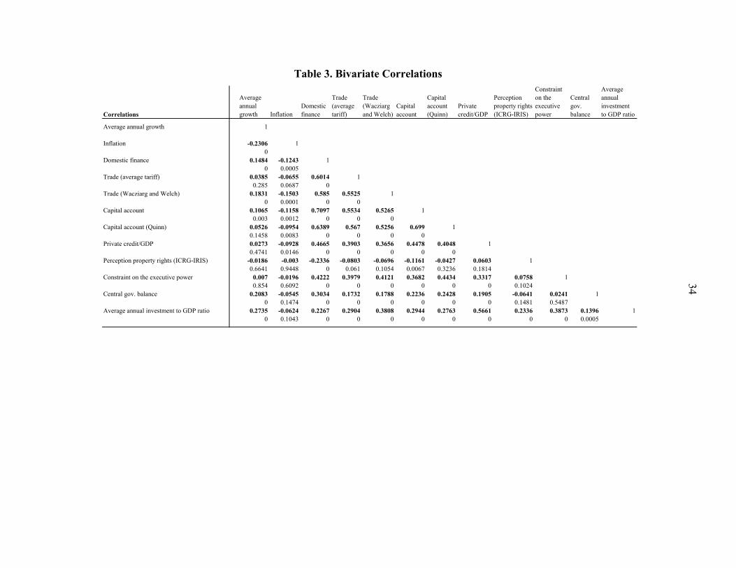
The baseline regression sample covers 90 countries over the period 1974-2004 (Table 1). The sample of countries ranges from low-income countries to high income countries and covers most emerging markets. Summary statistics reported in Table 2 show that real per capita GDP growth averaged 2 percent annually over the sample period, while investment to GDP averaged 17 percent over the period considered. As shown in Table 3, real per capita growth is significantly and positively correlated with the 3 main indices of structural reforms, in particular the domestic financial reform index, the Wacziarg and Welch index of trade and economic reforms, and the indicator of liberalization of cross-border financial credit (the capital account index). The correlation with the broader measure of capital account liberalization by Quinn (1997) is, however, not significant. Moreover, per-capita real GDP growth is also positively and significantly correlated with macroeconomic indicators (such as low inflation or the fiscal balance), but there is no significant correlation with the private credit to GDP ratio, or with indicators of institutional development (such as the constraint on the executive index, or the ICRG index of property rights development). As an additional initial exploration of the relationship between economic performance and indicators of reforms, we examine the evolution of per-capita real GDP growth during episodes

14

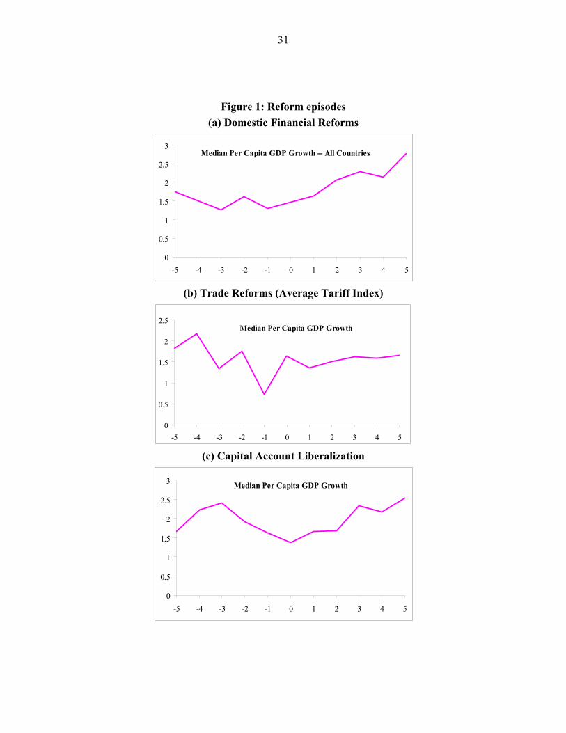
of reforms. For this purpose, and for each of the indicators of reforms (domestic finance, trade and the capital account), we define episodes of significant reforms as changes in the index corresponding to the top quartile of the distribution of the changes. We then plot the median per capita real GDP growth in the years surrounding the reform. The results are shown in Figure 1. Reforms of the domestic financial system seem to be associated with an acceleration of economic growth in the five years following the reform. In contrast, no clear changes in economic growth take place in the years following trade or capital account reforms. We next explore the relationship between economic performance and reforms more rigorously using our various empirical specifications.

V. MAIN RESULTS

A. Standard growth regressions

Table 4 reports estimation results for the standard growth regression specification described in section III, in which all three liberalization indices are included simultaneously. The first column reports the estimation on the complete sample of countries, while columns 2-4 report estimation results by income groups. Control variables in all regressions include the log of initial real per capita GDP, and the initial inflation rate. All specifications also include an interaction of each liberalization index with a dummy variable for transition countries to account for potentially different growth dynamics in these countries. Estimation results show that, among the three dimensions of liberalization considered, only domestic financial liberalization is significantly and positively associated with per capita GDP growth. In contrast, capital account and trade liberalization are not significantly associated with growth. Furthermore, the association between domestic financial liberalization and economic growth is strongly significant only for middle-income countries, and even more so for transition countries (column 3). In high income countries (column 2), the positive association is driven entirely by two transition countries (the Czech Republic and Estonia). In low income countries (column 4), the association between domestic finance and economic growth is weakly statistically significant. Finally, trade reforms seem positively associated with economic growth

15

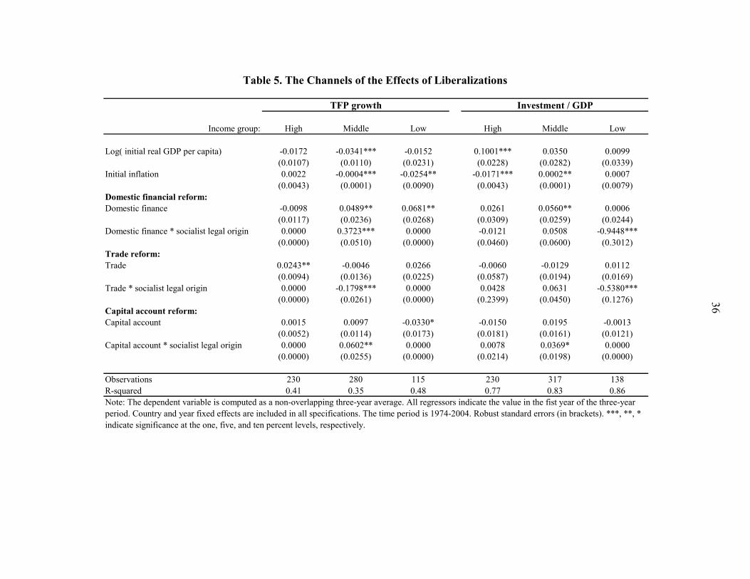
in high income countries while the coefficient on capital account liberalization is either not significant, or negatively associated with economic growth.9 In Table 5 we explore the channels through which liberalization is associated with better economic performance and test whether liberalizations affect the growth of total factor productivity and capital accumulation. For this purpose, we compute the Solow residual from a growth accounting exercise as a proxy for the growth of aggregate total factor productivity, which many papers have shown to be a main driver of long-term growth (see, e.g., Hall and Jones, 1999, and Beck et al., 2000).10 As a proxy for capital accumulation, we consider the ratio of gross capital formation to GDP. We find that domestic financial liberalization is positively and significantly associated both with TFP growth and aggregate investment in middle-income countries, and is positively associated with TFP growth in low-income countries. Hence, in developing economies structural reforms appear to be associated with both faster TFP growth and higher capital accumulation. General Method of Moment regressions, reported in Table 6, show that our results are robust to addressing endogeneity of domestic financial liberalization, capital account liberalization and trade liberalization. Following the technique developed by Arrelano and Bond (1991) and Blundell and Bond (1998), we use a GMM estimator to correct two biases: (i) the bias arising in a dynamic panel with fixed effects; and (ii) endogeneity bias. The table reports estimations based on the two-step system-GMM estimator corrected for heteroscedasticity and small sample bias (Windmeijer, 2004).11 Identification is based on the assumption that lags of the first difference of right-hand side (RHS) variables are valid instruments for levels of the RHS variables, and that lags of the levels of the RHS variables are valid instruments for the first difference of the RHS variables.12 We find that the positive association between domestic financial reforms and 9 The group of low-income transition countries–for which the coefficient on capital account liberalization is positive and significant–includes only 3 countries (the Kyrgyz Republic, Uzbekistan and Vietnam).

10 In the growth accounting exercise, we follow the approach in Bosworth and Collins (2003) by updating their data set based on the latest Penn World Tables.

11 The system GMM estimator is more appropriate than the difference GMM estimator when the country dimension is small. We report the first-step Sargan test of overidentifying restrictions, and autocorrelation tests of order 1, 2 and 3.

12 In the real GDP growth and TFP growth regression, we rely on the first lag of the first difference of RHS variables and third and fourth lags of the levels of the RHS variables as instruments. In the investment regression, we use respectively the second lag of the level, and the third and fourth lags of the first difference as instruments.

16

economic performance remains significant both in the real GDP per capita growth regression and in the TFP growth regression. However, significance falls below 10 percent in the investment regression. Overall, this analysis shows that, among three sets of reforms – domestic financial reforms, trade reforms and capital account reforms – domestic financial reforms are more robustly associated with improved economic performance (in particular TFP growth). Moreover, this association obtained in a standard growth setting is mainly driven by middle-income countries.

B. Dynamic Effects of Reforms

As discussed in section III, the standard growth regression specification does not allow us to test for more complex dynamics in the growth effects of reforms. The standard regressions shown so far assume a growth effect starting in the period after the liberalization index changes as well as linearity of growth effects in changes in the index; it does not allow to test for how persistent the effects of liberalizations on growth are. To analyze more complex patterns and the extent to which the effects of liberalizations on growth are persistent, we consider the specification described in equation (6) above. We consider episodes of reforms that occur during the period considered and reform episodes of the previous period, so we assess the effect of reforms over a maximum time span of 6 years. Our specification also includes indicators for reform reversals to test whether such events are associated with worsened economic performance. In robustness tests, we also include reform episodes that occurred two periods earlier, hence allowing us to test whether a reform has a lasting effect on economic growth 6 to 9 years after it occurred. Another advantage of this specification is that multi-collinearity across liberalizations–which may result in large standard errors–is less likely to be a concern. Indeed, while levels of the liberalization indices are quite strongly correlated with each other (Table 3), potentially as a result of country-specific trends, reform episodes rarely occur simultaneously during a three years period, and as a result, our reform episode indicators are not correlated.13

13 The correlations between domestic financial, trade and capital account reform episodes are between 0.05 and 0.13. Frequencies of domestic finance, trade and capital account reform episodes are respectively 8.3 percent, 7.8 percent and 16.2 percent. For large domestic finance and trade reform episodes, frequencies are 1.7 percent and 4.5 percent.

17

An additional concern in a standard growth regression is that reforms may occur after an improvement in economic performance (anticipatory effects, reverse causality). To capture such effects, we also include leads of reform episodes (i.e., indicator variables for periods that precede reform episodes). Lastly, in addition to the initial level of real GDP per capita and inflation, we also include dummies for banking crises, conflicts and episodes of hyperinflation as additional control variables. Estimation results are reported in Table 7. We find that in the complete sample of countries, neither domestic finance nor capital account reforms are significantly associated with faster economic growth. In contrast, trade reforms seem to be associated with higher economic growth both in the contemporaneous period and in the following period. Moreover, the coefficient on the lead of large trade reforms is significant and positive. This finding suggests that the estimated relationship between trade reforms and economic growth may reflect reverse causality: growth accelerates before trade reforms are actually implemented. An alternative interpretation is that economic agents anticipate reforms, and that these reform expectations affect economic performance positively. This interpretation is consistent with the fact that the lead-effect only holds for large reforms, which may be more likely to be anticipated. Lastly, reversals of capital account liberalization are significantly and negatively associated with contemporaneous economic growth, while capital account reforms are not symmetrically related to growth improvements, perhaps because reform reversals act as a (stronger) negative signal to investors. The finding also leaves room for interpretations in the reverse direction along the lines of Abiad and Mody (2005) who found that crises may cause reversals.14 Again, the significant association between reforms and economic performance is driven by the sub-sample of middle-income countries (column 3). We confirm that in this sub-sample of countries, trade reforms are positively and significantly associated with faster economic growth, and the effect is persistent at a six-year horizon. Large trade reforms, however, are not associated with higher economic growth than are small trade reforms, a finding that is potentially consistent with a reverse-causality explanation. In middle-income countries, episodes of domestic financial reforms are significantly associated with faster economic growth. The estimated effect of domestic financial reforms is economically

14 More precisely, Abiad and Mody (2005) find that balance-of-payments crises spurred reforms, while banking crises set liberalization back.

18

large: economic growth increases by 1.2 to 1.4 percentage points on average in the 3 to 6 years following a reform episode. Moreover, the estimated effect is even stronger for episodes of large domestic financial reforms, as economic growth increases by an additional 1.2 percentage points. Table 8 explores the channels underlying the association (or the lack thereof) between economic growth and reform episodes. The effect of domestic financial reforms on economic growth in middle-income countries seems to be explained mostly by a better use of factors of production rather than higher aggregate investment which increases only temporarily, and less significantly (columns 2 and 5). Interestingly, domestic finance reversals seem to be preceded by higher aggregate investment in these countries (column 5), which may be explained by an anticipation effect, with investors accelerating their projects before the expected reversal, or more broadly because reversals may be preceded by economic booms. Moreover, trade reforms are preceded by both faster TFP growth and aggregate investment in middle-income countries, and are associated with faster TFP growth, as well as higher aggregate investment in the case of large trade reforms. Finally, we mostly confirm the lack of a clear pattern between reform episodes and performance in high income and low income countries.

VI. ROBUSTNESS TESTS AND ENDOGENEITY

In this section, we conduct robustness tests on the estimated relationship between indicators of economic performance and structural reforms. First, we add controls for various factors that could affect economic performance. Second, we develop an instrumental variable strategy to further address endogeneity concerns.

A. Robustness tests

In Table 9, we investigate the robustness of the association between economic growth and

financial reforms in middle-income countries, by adding one by one a number of additional

control variables. We begin by adding an indicator of the quality of property rights, which has

been found to matter for long-run economic performance (Acemoglu and Johnson, 2005;

Easterly and Levine, 2003). Following this literature, we add the Polity IV “constraint on the

executive” index in column 1, in addition to our previous set of basic control variables. We also

include additional measures of the quality of macroeconomic management (in addition to the

previously included inflation rate) in columns 2 and 3: the fiscal balance, and a measure of real

exchange rate overvaluation (Fisher et al., 1996; Easterly and Levine, 2003). Our main

conclusions remain unchanged.

19

Next, in column 4 we test for whether the effect of domestic financial liberalization on economic

growth is through a deepening of the banking system by controlling for the ratio of private credit

to GDP (Levine, 1997, 2005). The effect of domestic financial reforms on economic growth

remains significant even after controlling for the stock of private credit to GDP during the period

considered, suggesting that financial reforms affect economic growth independently of the

volume of credit intermediated by the banking system. This finding is consistent with the

hypothesis that financial reforms affect growth not necessarily through a higher aggregate

volume of credit, but also through a better allocation of credit.

In column 5, we control for the quality of education–proxied by school enrolment rates–which

has been shown to matter for long-run economic performance (Mankiw, Romer and Weil, 1992).

Moreover, using a broader measure of trade and economic liberalization (due to Sachs and

Warner and extended and refined by Wacziarg and Welch, 2009) instead of an average tariff

index only slightly reduces the significance of the coefficient on lags of domestic financial

reform episodes (column 6).

Finally, we explore the persistence of the impact of domestic financial reform on economic

growth by adding reform episode dummies for reforms undertaken 6 to 9 years before the period

of observation (column 7). We find no persistent effect at this horizon, suggesting that domestic

financial reforms may not have direct long-run effects on economic growth, but only lasting

effects on the level of output on the order of 10 percent for a full liberalization after 6 years. This

finding does not preclude the possibility that financial reforms may also have indirect long-run

effects on economic performance by deepening domestic financial systems (Tressel and

Detragiache, 2008).

In table 10 we perform similar robustness tests for the channel regressions on TFP growth (panel

A) and aggregate investment (panel B). We confirm that aggregate TFP growth – rather than the

aggregate accumulation of capital – is the most robust channel through which domestic financial

and trade reforms are associated with higher economic growth.

B. Endogeneity

So far, our analysis has focused on establishing a robust association between economic

performance and indicators of structural reforms in middle-income countries, in the three areas

20

of domestic finance, trade and the capital account. As highlighted in the discussions of our

results, endogeneity is likely to be an important concern. In this section, we present an approach

to address such concerns, and to show that our main findings remain intact when implementing

an instrumental variable (IV) approach.

GMM regressions reported earlier already tackle endogeneity bias. Moreover, some aspects of

reverse causality are addressed by the inclusion of leads of the reform episode dummies. Indeed,

if reforms took place in countries that are experiencing growth accelerations, we would observe

that growth accelerates before the reforms are implemented. We find some evidence consistent

with this reverse causality for trade reforms, but no such evidence for domestic financial reforms.

However, it could be the case that reforms are implemented when the economy is expected to

perform well. More generally, omitted factors that are not observable may bias the estimates.

To further address these endogeneity concerns, we develop an IV strategy. The hypothesis for

the choice of instruments is that economic reforms diffuse across countries with close political

ties as a result of a learning or an imitation process. The conjecture is that, all else being equal, a

country is more likely to reform when political allies have already successfully implemented

similar policies, or are in the process of undertaking reforms. Thus, we use as an instrument for

reform episodes in a particular country the process of reform (in the same sector) of political

allies weighted by the “Entente Alliances” index. This index takes the value of 0 or 1 whenever

two countries are common members of, or signatories to, an entente or alliance in any given

period.15

Formally, for each sector S (domestic finance, capital account, and trade), we consider as

instruments for a reform episode SitReform , or large reform episode _ S

itLarge Reform , the levels of

the index 3,2,1,0, uS

utpolI and change in the index of political allies 3,2,1,0, uS

utpolI , of the same

period t and previous periods, with maximum of 3 lags. Furthermore, for the domestic financial

reform index, we use all the 6 components of the index instead of the aggregate index. The

exclusion restrictions – tested in the empirical analysis – are the following:

15 The index is from Rajan and Subramanian (2005). The original source is the Correlates of War Database.

21

,

,

, , _ 0

, , _ 0

Sit pol t u it it it

Sit pol t u it it it

E y I X Reform Large Reform

E y I X Reform Large Reform

for all 3,2,1,0u .

Hence, identification is based on the exclusion restrictions that levels and changes of the

liberalization index of political allies are uncorrelated with unobserved factors affecting

economic performance, conditional on the country reform process and control variables.

Tables 11a and b report 2SLS regression results for real GDP growth, TFP growth and

investment. Second stage regressions (Table 11a) confirm the result obtained with OLS for

domestic financial reforms. The coefficient on the domestic financial reform variables is

significant for real GDP growth and TFP growth, both for contemporaneous and previous period

reform episodes. Moreover, there is evidence of stronger effects on TFP growth of large reforms

in the previous period. In contrast, coefficients on trade reform variables become insignificant in

2SLS regressions, suggesting that the positive correlation obtained in our previously estimated

OLS regressions may reflect endogeneity bias. Finally, coefficients on capital account

liberalization remain insignificant.

Specification tests confirm the validity of the instruments. The null hypothesis of joint validity of

the instruments (Hansen J test) is not rejected at the 22 percent level, 15 percent level and 15

percent level respectively in the real per capita GDP growth, TFP growth and investment

equations. Moreover, the F tests of the first stage (Table 11b) confirm that our instruments are, in

general, reasonably strong.16

VII. REFORM SEQUENCING AND ECONOMIC PERFORMANCE

By splitting countries by income groups, we have established that structural reforms – in particular financial and to some extent trade reforms – have a discernable effect on real GDP growth mainly in middle-income countries. In this section, we explore whether the sequencing between various reforms may be a valid explanation for this finding. In particular, we focus on the sequencing between economic reforms on the one hand and political reforms on the other. 16 Stock and Yogo (2005) recommend a threshold of about 10 for the first stage F test to ensure that the results are not affected by weak instrument bias, under the criteria that the bias of the IV is less than 10 percent of the OLS bias.

22

A recent literature has shown that the effectiveness of economic reforms may depend on the broad institutional environment, in particular on political institutions and the protection of property rights (Acemoglu and Johnson, 2005; Acemoglu et al., 2008; Giavazzi and Tabellini, 2005; Levine, 2005; Tressel and Detragiache, 2008). This approach is also related to the literature trying to identify the constraints on growth (Rodrik, 2006; Hausman et al., 2005). We take a first step in testing whether a complementarity between economic reforms and the political environment may explain the lack of growth effects of reforms in some countries. For this purpose, we exclude advanced economies—as the previous results have shown, the reforms we are considering generally matter more for growth in developing economies, and the development of political institutions in particular was likely to be less relevant for most advanced economies in recent decades. We split the sample based on the median value of the constraint on the executive variable. This sample does not exactly correspond to the income group sample, even though middle-income countries are disproportionately represented in the sample of countries above the median, accounting for 80 percent of the countries with above-median developed political institutions. In the sample of below-median countries, middle-income countries account for roughly half (53 percent) of the sample, including middle-income countries such as Indonesia, Morocco and Tunisia. Table 12 reports growth regressions on the two-subsamples and robustness tests on the subsample of good property rights countries. Columns (1) and (2) show the baseline regressions on the good property rights sample, and on the bad property rights sample. We find that in countries with good property rights, domestic financial reforms seem to be associated with faster economic growth at a 6 years horizon. In contrast, we find no significant association in countries with bad property rights. Turning to trade and capital account reforms, we find some positive association between economic growth and trade reforms in the good property right sample, but continue to find no significant impact of capital account reforms in both sub-samples of countries. The results for domestic financial reforms (and to some extent trade reforms) are robust to the inclusion of various control variables (columns 3 to 7). Finally, we confirm the previous finding of a lack of a sustained impact of domestic financial reforms on economic growth beyond a 6 year horizon (column 7).17 Overall, the results suggest that sufficiently developed political institutions are a precondition for reaping the benefits of economic

17 Instrumental variable regressions reported in the appendix tend to support a causal interpretation of these findings.

23

reforms.18This finding is consistent with the finding of Acemoglu and Johnson (2005), but seems at odds with Giavazzi and Tabellini (2005)’s results. The positive relationship between domestic financial and trade reforms and economic growth in countries with good property rights again is explained by improvements in measured aggregate TFP growth, not by higher aggregate investment rates (results not reported). This finding is robust to the inclusion of various controls, and to endogeneity bias (appendix table).

VIII. CONCLUSION

In this paper, we have presented a new assessment of the growth benefits of various economic

reforms. While a large literature already exists on this topic, this paper adds to it by

simultaneously examining the effects of different types of economic reforms, as well as their

interactions with the quality of political institutions. Consistent with previous studies, we find

that domestic financial reforms are robustly associated with positive growth for up to 6 years

after the reform is implemented. Similar growth benefits arise from trade reforms, while capital

account reforms are not associated with faster growth. Interestingly, though, reversals of capital

account reforms are associated with slower growth. Lastly, we present evidence suggesting that

sufficiently developed property rights may be a necessary condition for reforms to be effective

and to stimulate economic performance. This finding may help explain the lack of reform effects

in some countries.

Most of our results are driven by middle-income countries. Understanding why this is the case is

an important area for future research. For example, do different reforms matter in high- and low-

income countries compared to middle-income countries? Our results on the importance of

property rights in developing economies go some way of answering this, but more work may be

needed in this direction. Also, while we have considered the sequencing between economic and

(a particular type of) political reforms, understanding whether other sequences among economic

18 These results are in contrast to those by Giavazzi and Tabellini (2005) who found that implementing economic (trade) reform before political reform is the reform sequence that would lead to better growth outcome.

24

reforms matter is another important question from a policy perspective. These issues are the

subject of ongoing research.19

19 Ostry et al. (2009) provide some initial results in this area.

25

References

Abiad, Abdul, Enrica Detragiache and Thierry Tressel, 2008, “A New Database of Financial

Reforms,” IMF Working Paper 08/266, IMF Staff Papers, 2009.

Abiad, Abdul, Nienke Oomes and Kenichi Ueda, 2008, “The Quality Effect: Does Financial

Liberalization Improve the Allocation of Capital?,” Journal of Development Economics

87(2), 270–282.

Abiad, Abdul, and Ashoka Mody, 2005, “Financial Reform: What Shakes It? What Shapes It?,”

American Economic Review 95(1), 66–88.

Acemoglu, Daron, and Simon Johnson, 2005, “Unbundling Institutions,” Journal of Political

Economy 113(5), 949–995.

Aghion, P., Howitt, P., and D. Mayer-Foulkes, 2005,"The Effect of Financial Development on

Convergence: Theory and Evidence", The Quarterly Journal of Economics.Arellano,

Manuel, and Stephen Bond , 1991, “Some Tests of Specification for Panel Data: Monte

Carlo Evidence and an Application to Employment Equations,” Review of Economic

Studies 58, 277–297.

Beck, T.H.L., Levine, R., & Loayza, N. (2000). Financial intermediation and growth: Causality

and causes. Journal of Monetary Economics, 46(1), 31-77.

Beck, T.H.L., Levine, R., & Loayza, N. (2000). Finance and the sources of growth. Journal of

Financial Economics, 58(1-2), 261-300.

Bekaert, Geert, and Campbell R. Harvey, 2000, “Foreign Speculators and Emerging Equity

Markets,” Journal of Finance 55, 565–613.

Bekaert, Geert, and Campbell R. Harvey and Christian Lundblad, 2003, “Equity Market

Liberalization in Emerging Markets,” Journal of Financial Research 26, 275–299.

Bekaert, Geert, Campbell R. Harvey and Christian Lundblad, 2005, “Does Financial

Liberalization Spur Growth?,” Journal of Financial Economics 77, 3–55.

26

Bhattacharya, Rina, 1997, “Pace, Sequencing and Credibility of Structural Reforms,” World

Development 25, 1045–1061.

Binici, Mahir, Michael Hutchison and Martin Schindler, 2009, “Controlling Capital? Legal

Restrictions and the Asset Composition of International Financial Flows,” IMF Working

Paper No. 09/208. Forthcoming in Journal of International Money and Finance.

Blundell, Richard, and Stephen Bond. (1998). “Initial Conditions and Moment Restrictions in

Dynamic Panel Data Models,” Journal of Econometrics 87, 115–143.

Bonfiglioli, Alessandra, 2008, “Financial Integration, Productivity and Capital Accumulation,”

Journal of International Economics 76, 337–355.

Bosworth, Barry, and Susan Collins (2003), “The Empirics of Growth: An Update,”

Braun, Matías, and Claudio Raddatz, 2007, “Trade Liberalization, Capital Account

Liberalization and the Real Effects of Financial Development,” Journal of International

Money and Finance 26, 730–761.

Campos, Nauro F., and Fabrizio Coricelli, 2009, “Financial Liberalization and Democracy: The

Role of Reform Reversals,” CEPR Discussion Paper No. 7393.

Chinn, Menzie, and Hiro Ito, 2006, “What Matters for Financial Development? Capital Controls,

Institutions, and Interactions,” Journal of Development Economics 61, 163-192.

Chinn, Menzie D., and Hiro Ito, 2007, “A New Measure of Financial Openness,” mimeo.

Downloaded from http://www.ssc.wisc.edu/~mchinn/research.html.

Clemens, Michael A., and Jeffrey G. Williamson, 2004, “Why Did the Tariff-Growth Correlation

Reverse after 1950?,” Journal of Economic Growth 9, 5–46.

Dell’Ariccia, Giovanni, Julian di Giovanni, André Faria, Ayhan Kose, Paolo Mauro, Jonathan

Ostry, Martin Schindler, and Marco Terrones, 2008, “Reaping the Benefits of Financial

Globalization,” IMF Occasional Paper 264, Washington, DC: International Monetary

Fund.

27

Desai, Mihir, C. Fritz Foley, and James Hines, 2006, “Capital Controls, Liberalizations, and

Foreign Direct Investment,” Review of Financial Studies 19, 1399–1431.

Dollar, David, and Aart Kraay, 2004, “Trade, Growth, and Poverty,” Economic Journal 114,

F22–F49.

Easterly, W., and R. Levine, 2003, "Tropics, germs, and crops: the role of endowments in

economic development",Journal of Monetary Economics, 50:1, January 2003.

Edison, Hali, Michael Klein, Luca Ricci, and Torsten Sløk, 2004, “Capital Account

Liberalization and Economic Performance: Survey and Synthesis,” IMF Staff Papers 51,

220–256.

Eichengreen, Barry, Ricardo Hausmann and Ugo Panizza, 2003, “Currency Mismatches, Debt

Intolerance and Original Sin: Why They Are Not The Same and Why It Matters,” NBER

Working Paper No. 10036.

Fischer, Stanley, Ratna Sahay and Carlos A. Vegh, 1996, “Stabilization and Growth in

Transition Economies: The Early Experience,” Journal of Economic Perspectives 10(2),

pp. 45–66

Forbes, Kristin J., 2007, “The Microeconomic Evidence on Capital Controls: No Free Lunch,” in

Sebastian Edwards, ed., Capital Controls and Capital Flows in Emerging Economics:

Policies, Practices, and Consequences, Chicago: The University of Chicago Press, 171–

199.

Giavazzi, Francesco, and Guido Tabellini (2005), “Economic and Political Liberalizations,”

Journal of Monetary Economics 52, 1297–1330.

Hall, Robert E., and Charles I. Jones, 1999, “Why Do Some Countries Produce So Much More

Output Per Worker Than Others?,” Quarterly Journal of Economics 114, 83–116.

Henry, Peter Blair, 2000a, “Do Stock Market Liberalizations Cause Investment Booms?,”

Journal of Financial Economics 58, 301–334.

28

Henry, Peter Blair, 2000b, “Stock Market Liberalization, Economic Reform, and Emerging

Market Equity Prices,” Journal of Finance 55, 529–564.

Henry, Peter Blair, 2003, “Capital Account Liberalization, the Cost of Capital, and Economic

Growth,” American Economic Review 93, 91–96.

Henry, Peter Blair, 2007, “Capital Account Liberalization: Theory, Evidence, and Speculation,”

Journal of Economic Literature 45, 887–935.

Klein, Michael W., and Giovanni P. Olivei, 2008, “Capital Account Liberalization, Financial

Depth, and Economic Growth,” Journal of International Money and Finance 27, 861–

875.

Kose, M. Ayhan, Eswar Prasad, Kenneth Rogoff and Shang-Jin Wei (2009), “Financial

Globalization: A Reappraisal,” IMF Staff Papers 56, 8–62.

Krueger, Anne O., 1997, “Trade Policy and Economic Development: How We Learn” The

American Economic Review 87(1) (Mar., 1997), pp. 1–22.

Levine, Ross, 1997, “Financial Development and Economic Growth: Views and Agenda,”

Journal of Economic Literature 35, 688-726.

Levine, Ross, 2005, “Finance and Growth: Theory and Evidence.” in Handbook of Economic

Growth, Eds:Philippe Aghion and Steven Durlauf, The Netherlands: Elsevier Science.

Mankiw, G., Romer, D., and D. Weil, 1992, "A Contribution to the Empirics of Economic

Growth", Quarterly Journal of Economics, 100, 225-251.

McKinnon, Ronald I. (1973), Money and Capital in Economic Development (Washington:

Brookings Institution).

McKinnon, Ronald I. (1993), The Order of Economic Liberalization: Financial Control in the

Transition to a Market Economy, (Baltimore: John Hopkins University)

29

Mody, Ashoka, and Antu Panini Murshid, 2005, Growing Up With Capital Flows, Journal of

International Economics 65, pp. 249–266.

Ostry, Jonathan, Alessandro Prati, Antonio Spilimbergo and an IMF staff team, 2009, “Structural

Reforms and Economic Performance in Advanced and Developing Countries,” IMF

Occasional Paper 268, Washington, DC: International Monetary Fund.

Prasad, Eswar, Kenneth Rogoff, Shang-Jin Wei, and M. Ayhan Kose, 2003, Effects of Financial

Globalization on Developing Countries: Some Empirical Evidence, IMF Occasional

Paper No. 220.

Prati, Alessandro, Martin Schindler and Patricio Valenzuela, 2009, “Who Benefits From Capital

Account Liberalization? Evidence From Firm-Level Credit Ratings Data,” IMF Working

Paper No. 09/210.

Quinn, Dennis P., 1997, The Correlates of Change in International Financial Regulation,

American Political Science Review 91, 531–551.

Quinn, Dennis P., and A. Maria Toyoda, “Does Capital Account Liberalization Lead to

Economic Growth?,” forthcoming in Review of Financial Studies.

Rajan, Raghuram, and Luigi Zingales, 1998, Financial Dependence and Growth, American

Economic Review 88, 559–586.

Rajan, Raghuram, and Luigi Zingales, 2003, “The Great Reversals: The Politics of Financial

Development in the Twentieth Century,” Journal of Financial Economics 69, 5–50.

Rajan, Raghuram, Subramanian, Arvind, and Eswar Prasad, 2007, “Foreign Capital and

Economic Growth”, Brookings Papers on Economic Activity, 2007 (1), 153-230.

Rodríguez, Francisco, and Dani Rodrik (2001), “Trade Policy and Economic Growth: A

Skeptic's Guide to the Cross-National Evidence,” Macroeconomics Annual 2000, eds.

Ben Bernanke and Kenneth S. Rogoff, MIT Press for NBER, Cambridge, MA.

30

Rodrik, Dani, and Arvind Subramanian, 2009, “Why Did Financial Globalization Disappoint?,”

IMF Staff Papers 56, 112–138.

Sachs, Jeffrey D., and Andrew Warner, 1995, “Economic Reform and the Process of Global

Integration,” Brookings Papers on Economic Activity 1:1–118.

Schindler, Martin, 2009, Measuring Financial Integration: A New Data Set, IMF Staff Papers 56,

222–238.

Galindo A., Schiantarelli, F., and A, Weiss, 2005, "Does Financial Liberalization Improve the

Allocation of Investment? Micro Evidence from Developing Countries" Journal of

Development Economics.

Shaw, Edward, 1973, Financial Deepening in Economic Development (New York: Oxford

University Press).

Stock, J. H., and M. Yogo, 2005, “Testing for Weak Instruments in IV Regression,” in

Identification and Inference for Econometric Models: A Festschrift in Honor of Thomas

Rothenberg, Cambridge University Press.

Subramanian, A., D. Rodrik, and F. Trebbi, 2004, “Institutions Rule: The Primacy of Institutions

Over Geography and Integration in Economic Development,” Journal of Economic

Growth, June, 9(2): pp.131-165.

Tressel, Thierry (2008), “Unbundling the Effects of Reforms,” Mimeo International Monetary

Fund.

Tressel, Thierry, and Enrica Detragiache (2008), “Do Financial Sector Reforms Lead to

Financial Development? Evidence from a New Dataset,” IMF Working Paper 08/265.

Wacziarg, Romain, and Karen Horn Welch (2008), “Trade Liberalization and Growth: New

Evidence,” World Bank Economic Review 22(2), 187-231.

Windmeijer, Frank, 2004, “A finite sample correction for the variance of linear efficient two-step

GMM estimators,” Journal of Econometrics.

31

Figure 1: Reform episodes

(a) Domestic Financial Reforms

(b) Trade Reforms (Average Tariff Index)

(c) Capital Account Liberalization

Median Per Capita GDP Growth -- All Countries

0

0.5

1

1.5

2

2.5

3

-5 -4 -3 -2 -1 0 1 2 3 4 5

Median Per Capita GDP Growth

0

0.5

1

1.5

2

2.5

-5 -4 -3 -2 -1 0 1 2 3 4 5

Median Per Capita GDP Growth

0

0.5

1

1.5

2

2.5

3

-5 -4 -3 -2 -1 0 1 2 3 4 5

32

Table 1. Country Sample

High Income Low Income

Australia Albania Mexico BangladeshAustria Algeria Morocco Burkina FasoBelgium Argentina Nicaragua Cote D'IvoireCanada Azerbaijan Paraguay EthiopiaCzech Rep Belarus Peru GhanaDenmark Bolivia Philippines IndiaEstonia Brazil Poland KenyaFinland Bulgaria Romania Kyrgyz RepFrance Cameroon Russia MadagascarGermany Chile South Africa MozambiqueGreece China Sri Lanka NepalHong Kong Colombia Thailand NigeriaIreland Costa Rica Tunisia PakistanIsrael Dominican Rep Turkey SenegalItaly Ecuador Ukraine TaiwanJapan Egypt Uruguay TanzaniaKorea El Salvador Venezuela UgandaNetherlands Georgia Viet NamNew Zealand Guatemala ZimbabweNorway HungaryPortugal IndonesiaSingapore JamaicaSpain JordanSweden KazakhstanSwitzerland LatviaUK LithuaniaUSA Malaysia

Middle Income

33

Table 2. Summary Statistics

Note: Summary statistics based on the sample of column 1, Table 7.

Variable Obs Mean Std. Dev. Min Max

Real per capita GDP growtgh 590 0.02 0.03 -0.13 0.17TFP growth 534 0.02 0.03 -0.10 0.10Investment / GDP 579 0.17 0.08 0.02 0.46Trade liberalization Index 584 0.72 0.22 0 1Domestic Financial Lib Index 590 0.51 0.29 0 1Capital Account Lib Index 590 0.59 0.37 0 1Inflation 589 41% 282% -10% 4770%Fiscal balance / GDP 517 -3.42 4.48 -25.11 13.81Banking crisis dummy 590 0.16 0.32 0 1External conflict dummy 590 0.07 0.23 0 1Private credit / GDP 533 0.41 0.35 0.01 1.97Constraint on the Executive 583 5.04 2.16 0 7Dummy inflation > 100 percent 590 0.03 0.18 0 1Domestic financial reform (Freq.) 590 0.37 0.48 0 1Large domestic financial reform (Freq.) 590 0.20 0.40 0 1Reversal of domestic financial reform (Freq.) 590 0.05 0.22 0 1Trade reform (Freq.) 590 0.21 0.41 0 1Large trade reform (Freq.) 590 0.05 0.22 0 1Reversal of trade reform (Freq.) 590 0.10 0.30 0 1Capital account reform (Freq.) 590 0.19 0.40 0 1Reversal of capital account reform (Freq.) 590 0.05 0.23 0 1RER overvaluation 590 -0.05 40.43 -153.84 160.50

34

Table 3. Bivariate Correlations

Correlations

Average annual growth Inflation

Domestic finance

Trade (average tariff)

Trade (Wacziarg and Welch)

Capital account

Capital account (Quinn)

Private credit/GDP

Perception property rights (ICRG-IRIS)

Constraint on the executive power

Central gov. balance

Average annual investment to GDP ratio

Average annual growth 1

Inflation -0.2306 10

Domestic finance 0.1484 -0.1243 10 0.0005

Trade (average tariff) 0.0385 -0.0655 0.6014 10.285 0.0687 0

Trade (Wacziarg and Welch) 0.1831 -0.1503 0.585 0.5525 10 0.0001 0 0

Capital account 0.1065 -0.1158 0.7097 0.5534 0.5265 10.003 0.0012 0 0 0

Capital account (Quinn) 0.0526 -0.0954 0.6389 0.567 0.5256 0.699 10.1458 0.0083 0 0 0 0

Private credit/GDP 0.0273 -0.0928 0.4665 0.3903 0.3656 0.4478 0.4048 10.4741 0.0146 0 0 0 0 0

Perception property rights (ICRG-IRIS) -0.0186 -0.003 -0.2336 -0.0803 -0.0696 -0.1161 -0.0427 0.0603 10.6641 0.9448 0 0.061 0.1054 0.0067 0.3236 0.1814

Constraint on the executive power 0.007 -0.0196 0.4222 0.3979 0.4121 0.3682 0.4434 0.3317 0.0758 10.854 0.6092 0 0 0 0 0 0 0.1024

Central gov. balance 0.2083 -0.0545 0.3034 0.1732 0.1788 0.2236 0.2428 0.1905 -0.0641 0.0241 10 0.1474 0 0 0 0 0 0 0.1481 0.5487

Average annual investment to GDP ratio 0.2735 -0.0624 0.2267 0.2904 0.3808 0.2944 0.2763 0.5661 0.2336 0.3873 0.1396 10 0.1043 0 0 0 0 0 0 0 0 0.0005

35

Table 4. Standard Growth Regressions

(1) (2) (3) (4)Dependent variable: GDP per capita growth All countries High Middle Low

Log( initial real GDP per capita) -0.0246*** -0.0303*** -0.0275*** -0.0059[0.0064] [0.0100] [0.0100] [0.0278]

Initial inflation -0.0004*** -0.0015 -0.0003*** -0.0237***[0.0001] [0.0043] [0.0001] [0.0051]

Domestic financial reform:Domestic finance 0.0291* 0.0004 0.0529** 0.0535*

[0.0147] [0.0126] [0.0243] [0.0295]Domestic finance * socialist legal origin 0.1629*** 0.1423*** 0.1644*** -0.0319

[0.0418] [0.0399] [0.0573] [0.0482]Trade reform:Trade 0.0050 0.0268* 0.0015 -0.0014

[0.0100] [0.0148] [0.0142] [0.0159]Trade * socialist legal origin 0.0351 0.0546 0.0431 -0.3610***

[0.0659] [0.3752] [0.0636] [0.1216]Capital account reform:Capital account 0.0073 -0.0012 0.0119 -0.0242**

[0.0060] [0.0071] [0.0098] [0.0112]Capital account * socialist legal origin -0.0248 -0.0101 -0.0254 0.3662**

[0.0158] [0.0087] [0.0223] [0.1494]

Observations 792 270 359 156R-squared 0.40 0.45 0.48 0.40

Income groups

Note: The dependent variable is computed as non-overlapping three-year averages of growth in real GDP per capita. All regressors indicate the value in the fist year of the three-year period. Country and year fixed effects are included in all specifications. The time period is 1974-2004. Robust standard errors (in brackets). ***, **, * indicate significance at the one, five, and ten percent levels, respectively.

36

Table 5. The Channels of the Effects of Liberalizations

Income group: High Middle Low High Middle Low

Log( initial real GDP per capita) -0.0172 -0.0341*** -0.0152 0.1001*** 0.0350 0.0099(0.0107) (0.0110) (0.0231) (0.0228) (0.0282) (0.0339)

Initial inflation 0.0022 -0.0004*** -0.0254** -0.0171*** 0.0002** 0.0007(0.0043) (0.0001) (0.0090) (0.0043) (0.0001) (0.0079)

Domestic financial reform:Domestic finance -0.0098 0.0489** 0.0681** 0.0261 0.0560** 0.0006

(0.0117) (0.0236) (0.0268) (0.0309) (0.0259) (0.0244)Domestic finance * socialist legal origin 0.0000 0.3723*** 0.0000 -0.0121 0.0508 -0.9448***

(0.0000) (0.0510) (0.0000) (0.0460) (0.0600) (0.3012)Trade reform:Trade 0.0243** -0.0046 0.0266 -0.0060 -0.0129 0.0112

(0.0094) (0.0136) (0.0225) (0.0587) (0.0194) (0.0169)Trade * socialist legal origin 0.0000 -0.1798*** 0.0000 0.0428 0.0631 -0.5380***

(0.0000) (0.0261) (0.0000) (0.2399) (0.0450) (0.1276)Capital account reform:Capital account 0.0015 0.0097 -0.0330* -0.0150 0.0195 -0.0013

(0.0052) (0.0114) (0.0173) (0.0181) (0.0161) (0.0121)Capital account * socialist legal origin 0.0000 0.0602** 0.0000 0.0078 0.0369* 0.0000

(0.0000) (0.0255) (0.0000) (0.0214) (0.0198) (0.0000)

Observations 230 280 115 230 317 138R-squared 0.41 0.35 0.48 0.77 0.83 0.86

TFP growth Investment / GDP

Note: The dependent variable is computed as a non-overlapping three-year average. All regressors indicate the value in the fist year of the three-year period. Country and year fixed effects are included in all specifications. The time period is 1974-2004. Robust standard errors (in brackets). ***, **, * indicate significance at the one, five, and ten percent levels, respectively.

37

Table 6. System GMM Regressions

(1) (2) (3)Dependent variable:

Log( initial real GDP per capita) -0.0127 -0.0136* 0.0123(0.0083) (0.0080) (0.0199)

Initial inflation -0.0005 -0.0005* 0.0001(0.0003) (0.0003) (0.0003)

Domestic financial reform:Domestic finance 0.0566** 0.0494** 0.0001

(0.0288) (0.0250) (0.0343)Domestic finance * socialist legal origin -0.0492 0.1977*** -0.1803

(0.0578) (0.0614) (0.1400)Trade reform:Trade -0.0402 -0.0367* -0.1156**

(0.0250) (0.0215) (0.0533)Trade * socialist legal origin 0.0905** -0.0265 0.1631

(0.0429) (0.0367) (0.1069)Capital account reform:Capital account 0.0134 0.0002 0.0356

(0.0109) (0.0095) (0.0221)Capital account * socialist legal origin 0.0059 0.0212 0.0636

(0.0224) (0.0230) (0.0507)

Observations 359 280 317Number of countries 44 31 44Sargan test (p-value) 0.11 0.96 0.99ar1 -2.76 -3.08 -2.78ar2 0.55 1.04 0.66ar3 -1.78 -1.17 -1.20

Note: Robust standard errors in parentheses, *** p<0.01, ** p<0.05, * p<0.1.

Real per capita GDP growth TFP growth Investment / GDP

38

 

(1) (2) (3) (4)Dep. variable: GDP per capita growth All countries Low Middle High

Domestic financial reform:

Contemporaneous reform 0.0017 0.0039 0.0122** -0.0079**[0.0032] [0.0091] [0.0060] [0.0038]

Large contemporaneous reform -0.0015 -0.0214* 0.0078 -0.0046[0.0033] [0.0112] [0.0058] [0.0042]

Contemporaneous reform reversal -0.0073 0.0022 -0.0031 0.0019[0.0064] [0.0201] [0.0094] [0.0081]

Reform (previous period) 0.0026 -0.0065 0.0143** -0.0004[0.0029] [0.0076] [0.0058] [0.0035]

Large reform (previous period) 0.0045 0.0020 0.0115* 0.0015[0.0037] [0.0147] [0.0063] [0.0038]

Reform reversal (previous period) 0.0047 -0.0207 0.0105 0.0101[0.0061] [0.0245] [0.0087] [0.0063]

Reform (following period) -0.0036 -0.0001 -0.0050 -0.0050[0.0031] [0.0098] [0.0056] [0.0032]

Large reform (following period) -0.0031 -0.0099 -0.0037 -0.0009[0.0041] [0.0124] [0.0067] [0.0046]

Reversal (following period) 0.0061 0.0258 0.0060 0.0116*[0.0067] [0.0196] [0.0092] [0.0066]

Trade reform:Contemporaneous reform 0.0081** -0.0033 0.0165*** 0.0063

[0.0034] [0.0101] [0.0059] [0.0056]Large contemporaneous reform 0.0014 -0.0176 0.0064 -0.0022

[0.0067] [0.0199] [0.0087] [0.0159]Contemporaneous reform reversal -0.0063 -0.0139 -0.0068 0.0052

[0.0060] [0.0148] [0.0072] [0.0126]Reform (previous period) 0.0101*** -0.0026 0.0154*** 0.0060

[0.0034] [0.0102] [0.0055] [0.0046]Large reform (previous period) -0.0053 -0.0309** 0.0049 0.0104

[0.0065] [0.0147] [0.0087] [0.0136]Reform reversal (previous period) -0.0022 -0.0115 0.0090 0.0013

[0.0044] [0.0109] [0.0063] [0.0100]

Reform (following period) 0.0055 0.0081 0.0101* -0.0008[0.0039] [0.0104] [0.0057] [0.0075]

Large reform (following period) 0.0187*** 0.0227 0.0189** 0.0000[0.0067] [0.0169] [0.0089] [0.0000]

Reversal (following period) -0.0032 -0.0022 0.0011 -0.0056[0.0055] [0.0104] [0.0085] [0.0072]

Table 7. Baseline: Dynamic Effect of Reforms

Income groups

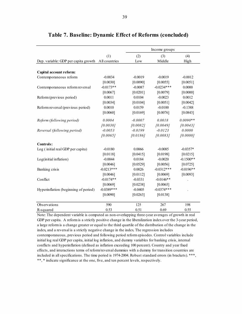
39

(1) (2) (3) (4)Dep. variable: GDP per capita growth All countries Low Middle High

Capital account reform:Contemporaneous reform -0.0034 -0.0019 -0.0019 -0.0012

[0.0030] [0.0090] [0.0055] [0.0051]Contemporaneous reform reversal -0.0173** -0.0087 -0.0234*** 0.0000

[0.0067] [0.0201] [0.0079] [0.0000]Reform (previous period) 0.0011 0.0104 -0.0023 0.0012

[0.0034] [0.0104] [0.0051] [0.0042]Reform reversal (previous period) 0.0010 0.0159 -0.0100 -0.1388

[0.0060] [0.0169] [0.0076] [0.0843]

Reform (following period) 0.0004 -0.0007 0.0018 0.0090**[0.0030] [0.0082] [0.0049] [0.0043]

Reversal (following period) -0.0053 -0.0199 -0.0123 0.0000[0.0065] [0.0186] [0.0083] [0.0000]

Controls:Log ( initial real GDP per capita) -0.0180 0.0066 -0.0085 -0.0357*

[0.0118] [0.0415] [0.0198] [0.0215]Log(initial inflation) -0.0044 0.0184 -0.0020 -0.1500**

[0.0046] [0.0529] [0.0056] [0.0725]Banking crisis -0.0213*** 0.0026 -0.0312*** -0.0196**

[0.0046] [0.0112] [0.0069] [0.0093]Conflict -0.0174** -0.0331 -0.0146** .

[0.0069] [0.0238] [0.0065]Hyperinflation (beginning of period) -0.0389*** -0.0405 -0.0374*** .

[0.0090] [0.0263] [0.0138]

Observations 590 125 267 198R-squared 0.53 0.51 0.69 0.55Note: The dependent variable is computed as non-overlapping three-year averages of growth in real GDP per capita. A reform is a strictly positive change in the liberalization index over the 3-year period, a large reform is a change greater or equal to the third quartile of the distribution of the change in the index, and a reversal is a strictly negative change in the index. The regression includes contemporaneous, previous period and following period reform episodes. Control variables include initial log real GDP per capita, initial log inflation, and dummy variables for banking crisis, internal conflicts and hyperinflation (defined as inflation exceeding 100 percent). Country and year fixed effects, and interactions terms of reform/reversal dummies with a dummy for transition countries are included in all specifications. The time period is 1974-2004. Robust standard errors (in brackets). ***, **, * indicate significance at the one, five, and ten percent levels, respectively.

Table 7. Baseline: Dynamic Effect of Reforms (concluded)

Income groups

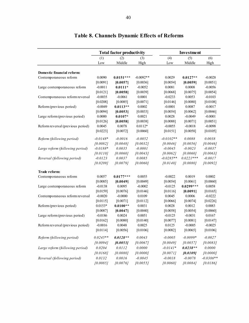
40

(1) (2) (3) (4) (5) (6)Low Middle High Low Middle High

Domestic financial reform:Contemporaneous reform 0.0090 0.0151*** -0.0092** 0.0029 0.0127** -0.0028

[0.0091] [0.0057] [0.0036] [0.0054] [0.0059] [0.0051]Large contemporaneous reform -0.0011 0.0111* -0.0052 0.0081 0.0008 -0.0056

[0.0121] [0.0058] [0.0039] [0.0068] [0.0075] [0.0054]Contemporaneous reform reversal -0.0035 -0.0061 0.0001 -0.0233 0.0053 -0.0103

[0.0208] [0.0085] [0.0071] [0.0146] [0.0080] [0.0108]Reform (previous period) -0.0049 0.0113** 0.0002 -0.0001 0.0087 -0.0017

[0.0094] [0.0053] [0.0033] [0.0054] [0.0062] [0.0046]Large reform (previous period) 0.0000 0.0107* 0.0021 0.0028 -0.0049 -0.0001

[0.0126] [0.0058] [0.0038] [0.0088] [0.0071] [0.0051]Reform reversal (previous period) 0.0045 0.0078 0.0112* -0.0055 -0.0018 -0.0098

[0.0223] [0.0072] [0.0060] [0.0151] [0.0058] [0.0105]

Reform (following period) -0.0148* -0.0016 -0.0052 -0.0102** 0.0088 0.0038[0.0082] [0.0048] [0.0032] [0.0046] [0.0056] [0.0046]

Large reform (following period) -0.0188* 0.0035 -0.0001 -0.0045 -0.0023 -0.0037[0.0110] [0.0060] [0.0043] [0.0062] [0.0060] [0.0063]

Reversal (following period) -0.0123 0.0037 0.0085 -0.0285** 0.0221*** -0.0017[0.0209] [0.0079] [0.0060] [0.0140] [0.0080] [0.0092]

Trade reform:Contemporaneous reform 0.0057 0.0177*** 0.0055 -0.0022 0.0019 0.0002

[0.0085] [0.0049] [0.0049] [0.0054] [0.0061] [0.0060]Large contemporaneous reform -0.0138 0.0095 -0.0002 -0.0125 0.0299*** 0.0058

[0.0159] [0.0076] [0.0146] [0.0116] [0.0091] [0.0165]Contemporaneous reform reversal -0.0020 -0.0000 0.0109 0.0045 0.0006 -0.0222

[0.0115] [0.0071] [0.0112] [0.0066] [0.0074] [0.0226]Reform (previous period) 0.0153* 0.0100** 0.0031 0.0028 0.0012 0.0083

[0.0087] [0.0047] [0.0040] [0.0058] [0.0054] [0.0060]Large reform (previous period) -0.0186 0.0024 0.0051 -0.0125 -0.0031 0.0167

[0.0162] [0.0080] [0.0140] [0.0077] [0.0081] [0.0147]Reform reversal (previous period) -0.0016 0.0048 0.0025 0.0125 -0.0005 -0.0025

[0.0114] [0.0056] [0.0106] [0.0082] [0.0065] [0.0106]

Reform (following period) 0.0245** 0.0128** 0.0043 -0.0005 -0.0099* -0.0027

[0.0094] [0.0053] [0.0067] [0.0049] [0.0057] [0.0083]

Large reform (following period) 0.0204 0.0112 0.0000 -0.0141* 0.0238** 0.0000[0.0168] [0.0080] [0.0000] [0.0071] [0.0109] [0.0000]

Reversal (following period) 0.0132 0.0016 -0.0045 -0.0018 -0.0078 -0.0386**[0.0085] [0.0076] [0.0055] [0.0060] [0.0084] [0.0186]

Table 8. Channels Dynamic Effects of Reforms

Total factor productivity Investment

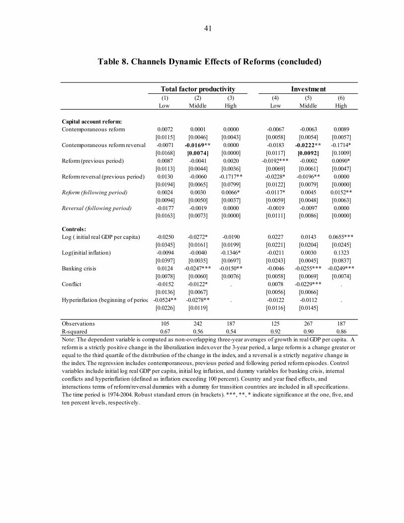
41

(1) (2) (3) (4) (5) (6)Low Middle High Low Middle High

Capital account reform:Contemporaneous reform 0.0072 0.0001 0.0000 -0.0067 -0.0063 0.0089

[0.0115] [0.0046] [0.0043] [0.0058] [0.0054] [0.0057]Contemporaneous reform reversal -0.0071 -0.0169** 0.0000 -0.0183 -0.0222** -0.1714*

[0.0168] [0.0074] [0.0000] [0.0117] [0.0092] [0.1009]Reform (previous period) 0.0087 -0.0041 0.0020 -0.0192*** -0.0002 0.0090*

[0.0113] [0.0044] [0.0036] [0.0069] [0.0061] [0.0047]Reform reversal (previous period) 0.0130 -0.0060 -0.1717** -0.0228* -0.0196** 0.0000

[0.0194] [0.0065] [0.0799] [0.0122] [0.0079] [0.0000]Reform (following period) 0.0024 0.0030 0.0066* -0.0117* 0.0045 0.0152**

[0.0094] [0.0050] [0.0037] [0.0059] [0.0048] [0.0063]Reversal (following period) -0.0177 -0.0019 0.0000 -0.0019 -0.0097 0.0000

[0.0163] [0.0073] [0.0000] [0.0111] [0.0086] [0.0000]

Controls:Log ( initial real GDP per capita) -0.0250 -0.0272* -0.0190 0.0227 0.0143 0.0655***

[0.0345] [0.0161] [0.0199] [0.0221] [0.0204] [0.0245]Log(initial inflation) -0.0094 -0.0040 -0.1346* -0.0211 0.0030 0.1323

[0.0397] [0.0035] [0.0697] [0.0243] [0.0045] [0.0837]Banking crisis 0.0124 -0.0247*** -0.0150** -0.0046 -0.0255*** -0.0249***

[0.0078] [0.0060] [0.0076] [0.0058] [0.0069] [0.0074]Conflict -0.0152 -0.0122* . 0.0078 -0.0229*** .

[0.0136] [0.0067] [0.0056] [0.0066]Hyperinflation (beginning of period -0.0524** -0.0278** . -0.0122 -0.0112 .

[0.0226] [0.0119] [0.0116] [0.0145]

Observations 105 242 187 125 267 187R-squared 0.67 0.56 0.54 0.92 0.90 0.86Note: The dependent variable is computed as non-overlapping three-year averages of growth in real GDP per capita. A reform is a strictly positive change in the liberalization index over the 3-year period, a large reform is a change greater or equal to the third quartile of the distribution of the change in the index, and a reversal is a strictly negative change in the index. The regression includes contemporaneous, previous period and following period reform episodes. Control variables include initial log real GDP per capita, initial log inflation, and dummy variables for banking crisis, internal conflicts and hyperinflation (defined as inflation exceeding 100 percent). Country and year fixed effects, and interactions terms of reform/reversal dummies with a dummy for transition countries are included in all specifications. The time period is 1974-2004. Robust standard errors (in brackets). ***, **, * indicate significance at the one, five, and ten percent levels, respectively.

Table 8. Channels Dynamic Effects of Reforms (concluded)

Total factor productivity Investment

42

Sample: Middle Income countries (1) (2) (3) (4) (5) (6) (7)

Dep. variable: GDP per capita growth

Property rights

Fiscal balance

Overvalued RER

Private credit to

GDPEducation

Economic liberalization (Wacziargand Welch)

Long lags

Domestic financial reform:Contemporaneous reform 0.0121** 0.0096 0.0118* 0.0100 0.0130* 0.0059 0.0095

[0.0061] [0.0066] [0.0062] [0.0062] [0.0067] [0.0067] [0.0064]Large contemporaneous reform 0.0079 0.0033 0.0072 0.0052 0.0109 0.0021 0.0043

[0.0057] [0.0060] [0.0058] [0.0056] [0.0075] [0.0076] [0.0058]Contemporaneous reform reversal -0.0025 -0.0057 -0.0033 -0.0054 -0.0012 -0.0065 0.0008

[0.0095] [0.0106] [0.0094] [0.0100] [0.0101] [0.0109] [0.0098]Reform (previous period) 0.0137** 0.0132** 0.0144** 0.0137** 0.0144** 0.0114* 0.0133**

[0.0059] [0.0065] [0.0058] [0.0068] [0.0065] [0.0059] [0.0066]Large reform (previous period) 0.0119* 0.0047 0.0114* 0.0075 0.0133* 0.0116 0.0082

[0.0063] [0.0064] [0.0062] [0.0066] [0.0068] [0.0070] [0.0067]Reform reversal (previous period) 0.0105 0.0079 0.0112 0.0077 0.0044 0.0084 0.0171*

[0.0088] [0.0070] [0.0086] [0.0070] [0.0088] [0.0082] [0.0096]

Reform (following period) -0.0049 -0.0039 -0.0053 -0.0020 -0.0032 -0.0044 -0.0109**[0.0056] [0.0058] [0.0056] [0.0054] [0.0062] [0.0051] [0.0055]

Large reform (following period) -0.0032 -0.0087 -0.0042 -0.0023 -0.0036 -0.0038 -0.0093[0.0068] [0.0071] [0.0067] [0.0068] [0.0071] [0.0087] [0.0069]

Reversal (following period) 0.0068 -0.0047 0.0059 0.0011 0.0035 -0.0077 -0.0037[0.0093] [0.0095] [0.0091] [0.0091] [0.0095] [0.0134] [0.0100]

Trade reform:Contemporaneous reform 0.0161*** 0.0183*** 0.0166*** 0.0202*** 0.0185*** 0.0021 0.0138**

[0.0060] [0.0062] [0.0059] [0.0059] [0.0067] [0.0063] [0.0064]Large contemporaneous reform 0.0062 0.0066 0.0070 0.0100 0.0113 0.0015

[0.0087] [0.0084] [0.0089] [0.0082] [0.0097] [0.0088]Contemporaneous reform reversal -0.0079 -0.0132** -0.0064 -0.0141** -0.0057 -0.0041

[0.0075] [0.0064] [0.0073] [0.0064] [0.0075] [0.0081]Reform (previous period) 0.0150*** 0.0154*** 0.0154*** 0.0153*** 0.0145** 0.0052 0.0174***

[0.0055] [0.0050] [0.0054] [0.0049] [0.0066] [0.0062] [0.0055]Large reform (previous period) 0.0047 0.0107 0.0048 0.0092 -0.0021 0.0069

[0.0087] [0.0091] [0.0087] [0.0090] [0.0088] [0.0092]Reform reversal (previous period) 0.0080 0.0054 0.0087 0.0035 0.0093 0.0135*

[0.0064] [0.0062] [0.0062] [0.0058] [0.0068] [0.0069]

Reform (following period) 0.0097* 0.0070 0.0097* 0.0123** 0.0105* -0.0048 0.0062[0.0056] [0.0055] [0.0059] [0.0057] [0.0058] [0.0076] [0.0061]

Large reform (following period) 0.0183** 0.0136 0.0200** 0.0217*** 0.0122 0.0097[0.0088] [0.0085] [0.0087] [0.0074] [0.0099] [0.0110]

Reversal (following period) -0.0002 -0.0149 0.0008 -0.0117 0.0013 0.0048[0.0084] [0.0093] [0.0084] [0.0089] [0.0094] [0.0087]

Capital account reform:Contemporaneous reform -0.0017 0.0024 -0.0018 0.0026 -0.0002 0.0013 -0.0004

[0.0056] [0.0061] [0.0054] [0.0055] [0.0061] [0.0064] [0.0058]Contemporaneous reform reversal -0.0229*** -0.0164* -0.0244*** -0.0165** -0.0248*** -0.0110 -0.0264***

[0.0080] [0.0085] [0.0082] [0.0080] [0.0091] [0.0115] [0.0093]Reform (previous period) -0.0023 0.0010 -0.0022 0.0011 0.0026 -0.0017 -0.0035

[0.0052] [0.0054] [0.0051] [0.0051] [0.0057] [0.0063] [0.0054]

Table 9. Robustness Tests Dynamic Effect of Reforms

Control variable

43

Sample: Middle Income countries (1) (2) (3) (4) (5) (6) (7)

Dep. variable: GDP per capita growth

Property rights

Fiscal balance

Overvalued RER

Private credit to

GDPEducation

Economic liberalization (Wacziargand Welch)

Long lags

Reform reversal (previous period) -0.0091 -0.0071 -0.0106 -0.0081 -0.0108 -0.0065 -0.0090[0.0078] [0.0079] [0.0078] [0.0068] [0.0086] [0.0064] [0.0068]

Reform (following period) 0.0018 0.0064 0.0023 0.0060 0.0057 0.0017 0.0025[0.0050] [0.0050] [0.0049] [0.0046] [0.0057] [0.0055] [0.0050]

Reversal (following period) -0.0115 -0.0108 -0.0123 -0.0130 -0.0084 0.0054 -0.0087[0.0085] [0.0089] [0.0084] [0.0080] [0.0092] [0.0098] [0.0087]

Control:Constraint on the executive 0.0014

[0.0015]Central government balance to GDP 0.0009

[0.0006]Overvaluation (Penn World Table) -0.0001

[0.0001]Private credit to GDP -0.0146

[0.0206]Primary school enrolment -0.0194

[0.0321]Secondary school enrolment -0.0827**

[0.0372]Tertiary school enrolment 0.0020

[0.0652]Financial reform (two periods before) 0.0034

[0.0055]Large financial reform (two periods before) -0.0024

[0.0052]Financial reform reversal (two periods before) 0.0029

[0.0078]

Observations 267 230 267 233 242 198 225R-squared 0.69 0.73 0.69 0.67 0.73 0.71 0.70Note: The dependent variable is computed as non-overlapping three-year averages of growth in real GDP per capita. A reform is a strictly positive change in the liberalization index over the 3-year period, a large reform is a change greater or equal to the third quartile of the distribution of the change in the index, and a reversal is a strictly negative change in the index. The regression includes contemporaneous, previous period and following period reform episodes. Control variables include initial log real GDP per capita, initial log inflation, and dummy variables for banking crisis, internal conflicts and hyperinflation (defined as inflation exceeding 100 percent). Country and year fixed effects, and interactions terms of reform/reversal dummies with a dummy for transition countries are included in all specifications. The time period is 1974-2004. Robust standard errors (in brackets). ***, **, * indicate significance at the one, five, and ten percent levels, respectively.

Table 9. Robustness Tests Dynamic Effect of Reforms (concluded)

Control variable

44

Dependent variable:

Sample: Middle-Income countriProperty

rightsFiscal

balancePrivate credit

to GDPOvervalued

RERProperty

rightsFiscal

balancePrivate credit

to GDPOvervalued

RER

Domestic financial reform:Contemporaneous reform 0.0149*** 0.0134** 0.0150** 0.0146** 0.0125** 0.0089 0.0081 0.0142**

[0.0056] [0.0059] [0.0061] [0.0059] [0.0059] [0.0058] [0.0059] [0.0057]Large contemporaneous reform 0.0112* 0.0094 0.0095 0.0104* 0.0009 0.0034 0.0024 0.0029

[0.0058] [0.0057] [0.0058] [0.0059] [0.0076] [0.0084] [0.0085] [0.0074]Contemporaneous reform reversal -0.0053 -0.0067 -0.0079 -0.0063 0.0057 0.0120 0.0081 0.0060

[0.0087] [0.0092] [0.0088] [0.0085] [0.0080] [0.0078] [0.0079] [0.0079]Reform (previous period) 0.0104** 0.0109* 0.0120** 0.0114** 0.0083 0.0069 0.0055 0.0082

[0.0053] [0.0057] [0.0060] [0.0052] [0.0061] [0.0064] [0.0062] [0.0060]Large reform (previous period) 0.0112* 0.0072 0.0073 0.0106* -0.0046 -0.0034 -0.0049 -0.0045

[0.0057] [0.0059] [0.0059] [0.0057] [0.0071] [0.0074] [0.0076] [0.0070]Reform reversal (previous period) 0.0078 0.0093 0.0086 0.0086 -0.0018 -0.0029 -0.0039 -0.0042

[0.0073] [0.0068] [0.0065] [0.0071] [0.0059] [0.0073] [0.0068] [0.0058]Reform (following period) -0.0015 -0.0014 0.0010 -0.0020 0.0089 0.0082 0.0076 0.0100*

[0.0048] [0.0051] [0.0049] [0.0049] [0.0056] [0.0058] [0.0056] [0.0053]Large reform (following period) 0.0042 -0.0014 0.0028 0.0029 -0.0019 -0.0026 -0.0016 -0.0002

[0.0061] [0.0059] [0.0058] [0.0062] [0.0061] [0.0070] [0.0068] [0.0060]Reversal (following period) 0.0049 -0.0066 -0.0021 0.0036 0.0227*** 0.0236** 0.0220** 0.0223***

[0.0080] [0.0078] [0.0079] [0.0078] [0.0080] [0.0092] [0.0086] [0.0080]

Trade reform:Contemporaneous reform 0.0170*** 0.0190*** 0.0211*** 0.0178*** 0.0016 0.0002 -0.0010 0.0017

[0.0049] [0.0051] [0.0050] [0.0049] [0.0061] [0.0064] [0.0063] [0.0061]Large contemporaneous reform 0.0092 0.0132 0.0149** 0.0101 0.0297*** 0.0267** 0.0258** 0.0279***

[0.0075] [0.0081] [0.0074] [0.0078] [0.0090] [0.0110] [0.0104] [0.0091]Contemporaneous reform reversal -0.0017 -0.0101 -0.0099 0.0006 -0.0003 0.0020 0.0012 -0.0011

[0.0073] [0.0063] [0.0062] [0.0071] [0.0076] [0.0088] [0.0082] [0.0071]Reform (previous period) 0.0093** 0.0096** 0.0098** 0.0099** 0.0008 0.0012 -0.0011 0.0014

[0.0047] [0.0045] [0.0044] [0.0047] [0.0054] [0.0058] [0.0053] [0.0053]Large reform (previous period) 0.0020 0.0090 0.0077 0.0022 -0.0034 -0.0035 -0.0070 -0.0025

[0.0081] [0.0085] [0.0082] [0.0081] [0.0080] [0.0088] [0.0087] [0.0080]Reform reversal (previous period) 0.0033 0.0019 0.0011 0.0045 -0.0013 0.0002 0.0000 0.0006

[0.0056] [0.0057] [0.0051] [0.0056] [0.0069] [0.0077] [0.0070] [0.0064]Reform (following period) 0.0122** 0.0105** 0.0156*** 0.0124** -0.0102* -0.0129** -0.0094 -0.0086

[0.0052] [0.0049] [0.0055] [0.0055] [0.0058] [0.0064] [0.0062] [0.0057]Large reform (following period) 0.0102 0.0042 0.0105 0.0125 0.0233** 0.0192 0.0162 0.0198*

[0.0080] [0.0077] [0.0078] [0.0078] [0.0108] [0.0126] [0.0114] [0.0106]Reversal (following period) -0.0005 -0.0116 -0.0084 0.0012 -0.0090 -0.0097 -0.0099 -0.0065

[0.0075] [0.0084] [0.0081] [0.0076] [0.0087] [0.0095] [0.0094] [0.0085]

Table 10. Dynamic Effect of Reforms on TFP and Investment Robusteness

Panel A: TFP growth Panel B: Investment / GDP

45

Dependent variable:

Sample: Middle-Income countriProperty rights Fiscal balance

Private credit to GDP

Overvalued RER

Property rights Fiscal balancePrivate credit

to GDPOvervalued

RER

Capital account reform:Contemporaneous reform 0.0005 0.0033 0.0040 0.0003 -0.0061 -0.0057 -0.0053 -0.0067

[0.0047] [0.0050] [0.0044] [0.0046] [0.0055] [0.0059] [0.0056] [0.0054]Contemporaneous reform reversal -0.0160** -0.0109 -0.0085 -0.0180** -0.0217** -0.0177* -0.0177** -0.0189**

[0.0075] [0.0078] [0.0075] [0.0076] [0.0090] [0.0099] [0.0088] [0.0090]Reform (previous period) -0.0041 -0.0013 -0.0003 -0.0040 -0.0002 -0.0032 -0.0026 -0.0005

[0.0045] [0.0046] [0.0044] [0.0044] [0.0061] [0.0063] [0.0065] [0.0059]Reform reversal (previous period) -0.0046 -0.0031 -0.0016 -0.0067 -0.0188** -0.0206** -0.0214** -0.0173**

[0.0066] [0.0074] [0.0063] [0.0067] [0.0080] [0.0099] [0.0084] [0.0076]Reform (following period) 0.0030 0.0082 0.0080 0.0036 0.0045 0.0029 0.0032 0.0027

[0.0051] [0.0054] [0.0049] [0.0052] [0.0048] [0.0057] [0.0053] [0.0049]Reversal (following period) -0.0007 -0.0005 -0.0018 -0.0019 -0.0091 -0.0079 -0.0068 -0.0097

[0.0075] [0.0080] [0.0073] [0.0073] [0.0087] [0.0098] [0.0089] [0.0084]Constraint on the executive 0.0021 0.0011

[0.0014] [0.0016]Central government balance / GDP 0.0000 -0.0008

[0.0004] [0.0007]Private credit to GDP -0.0234 -0.0113

[0.0186] [0.0240]Overvaluation (Penn World Table) -0.0001 0.0002***

[0.0001] [0.0001]

Observations 242 211 214 242 267 230 233 267R-squared 0.56 0.59 0.58 0.56 0.90 0.91 0.91 0.91Note: The dependent variable is computed as non-overlapping three-year averages of growth in real GDP per capita. A reform is a strictly positive change in the liberalization index over the 3-year period, a large reform is a change greater or equal to the third quartile of the distribution of the change in the index, and a reversal is a strictly negative change in the index. The regression includes contemporaneous, previous period and following period reform episodes. Control variables include initial log real GDP per capita, initial log inflation, and dummy variables for banking crisis, internal conflicts and hyperinflation (defined as inflation exceeding 100 percent). Country and year fixed effects, and interactions terms of reform/reversal dummies with a dummy for transition countries are included in all specifications. The time period is 1974-2004. Robust standard errors (in brackets). ***, **, * indicate significance at the one, five, and ten percent levels, respectively.

Table 10. Dynamic effect of reforms on TFP and Investment Robustness (concluded)

Panel A: TFP growth Panel B: Investment / GDP

46

Dependent variable is:

Domestic financial reform:Contemporaneous reform 0.0179** 0.0326*** -0.0054

[0.0083] [0.0085] [0.0097]Large contemporaneous reform 0.0092 0.0133 -0.0136

[0.0095] [0.0106] [0.0137]Contemporaneous reform reversal -0.0284 -0.0114 -0.0198

[0.0198] [0.0206] [0.0202]Reform (previous period) 0.0300*** 0.0274*** 0.0182*

[0.0099] [0.0106] [0.0108]Large reform (previous period) 0.0132 0.0228** -0.0187

[0.0102] [0.0102] [0.0118]Reform reversal (previous period) -0.0089 0.0173 -0.0217

[0.0187] [0.0167] [0.0183]

Reform (following period) 0.0098 0.0164* -0.0080[0.0086] [0.0091] [0.0101]

Large reform (following period) -0.0028 0.0090 -0.0025[0.0119] [0.0110] [0.0118]

Reversal (following period) 0.0203 0.0121 -0.0015[0.0192] [0.0177] [0.0204]

Trade reform:Contemporaneous reform 0.0134 0.0148 -0.0081

[0.0093] [0.0092] [0.0092]Large contemporaneous reform -0.0191 -0.0003 0.0110

[0.0167] [0.0160] [0.0204]Contemporaneous reform reversal -0.0100 -0.0009 0.0043

[0.0121] [0.0115] [0.0148]Reform (previous period) 0.0144* 0.0068 -0.0017

[0.0087] [0.0093] [0.0108]Large reform (previous period) 0.0087 -0.0125 0.0034

[0.0159] [0.0155] [0.0169]Reform reversal (previous period) 0.0259** 0.0016 0.0267**

[0.0117] [0.0113] [0.0120]

Reform (following period) 0.0129 0.0128 -0.0130[0.0094] [0.0089] [0.0097]

Large reform (following period) 0.0214 -0.0013 0.0210[0.0167] [0.0149] [0.0194]

Reversal (following period) -0.0047 -0.0152 -0.0133[0.0167] [0.0149] [0.0170]

Table 11a. Instrumental Variables Regressions

Real per capita GDP growth TFP growth Investment /GDP

Second Stage

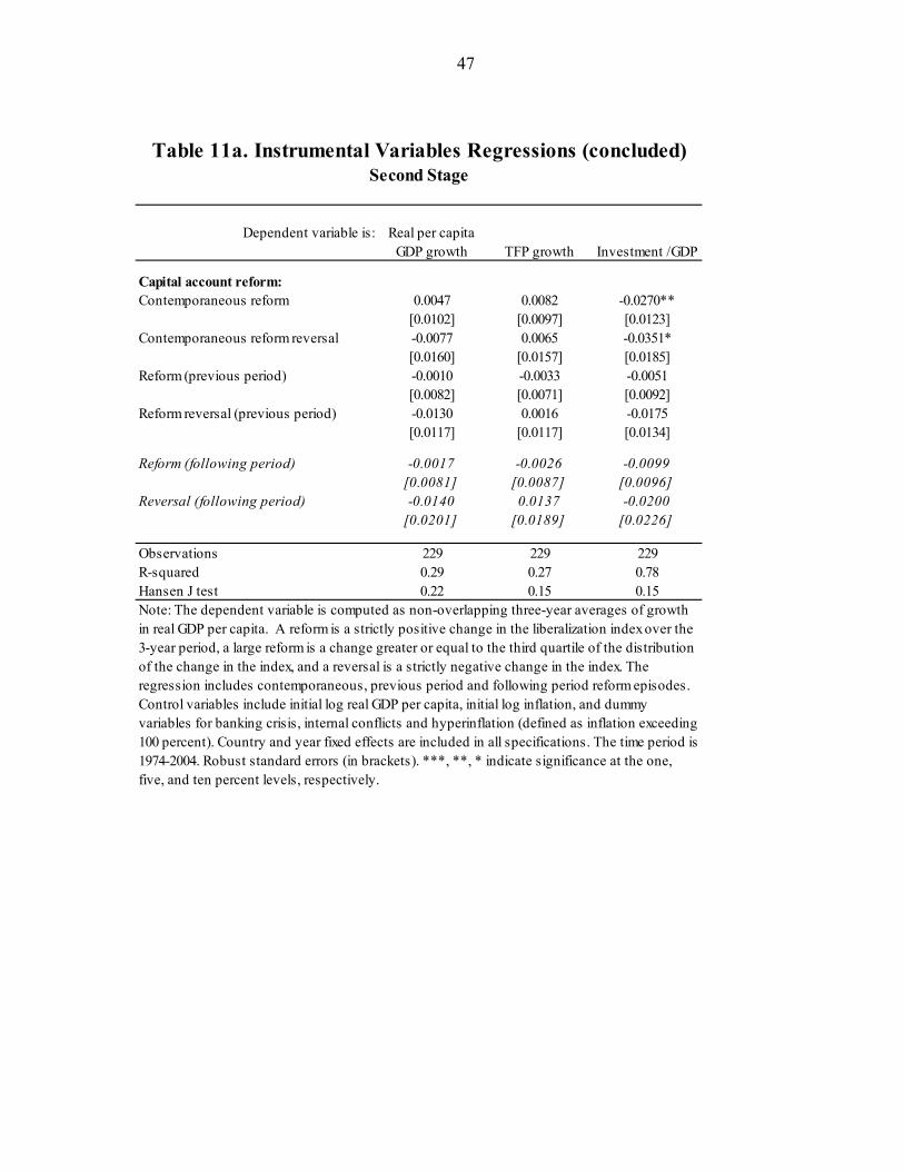
47

Dependent variable is:

Capital account reform:Contemporaneous reform 0.0047 0.0082 -0.0270**

[0.0102] [0.0097] [0.0123]Contemporaneous reform reversal -0.0077 0.0065 -0.0351*

[0.0160] [0.0157] [0.0185]Reform (previous period) -0.0010 -0.0033 -0.0051

[0.0082] [0.0071] [0.0092]Reform reversal (previous period) -0.0130 0.0016 -0.0175

[0.0117] [0.0117] [0.0134]

Reform (following period) -0.0017 -0.0026 -0.0099[0.0081] [0.0087] [0.0096]

Reversal (following period) -0.0140 0.0137 -0.0200[0.0201] [0.0189] [0.0226]

Observations 229 229 229R-squared 0.29 0.27 0.78Hansen J test 0.22 0.15 0.15

Investment /GDP

Note: The dependent variable is computed as non-overlapping three-year averages of growth in real GDP per capita. A reform is a strictly positive change in the liberalization index over the 3-year period, a large reform is a change greater or equal to the third quartile of the distribution of the change in the index, and a reversal is a strictly negative change in the index. The regression includes contemporaneous, previous period and following period reform episodes. Control variables include initial log real GDP per capita, initial log inflation, and dummy variables for banking crisis, internal conflicts and hyperinflation (defined as inflation exceeding 100 percent). Country and year fixed effects are included in all specifications. The time period is 1974-2004. Robust standard errors (in brackets). ***, **, * indicate significance at the one, five, and ten percent levels, respectively.

Table 11a. Instrumental Variables Regressions (concluded)Second Stage

Real per capita GDP growth TFP growth

48

Endogenous variable Partial R2 F testF(61, 125)

Domestic financial reform:

Contemporaneous reform 0.40 8.0Large contemporaneous reform 0.35 10.2Contemporaneous reform reversal 0.24 0.7

Reform (previous period) 0.35 10.4Large reform (previous period) 0.49 7.1Reform reversal (previous period) 0.23 0.8

Reform (following period) 0.35 6.6Large reform (following period) 0.39 10.3Reversal (following period) 0.18 0.4

Trade reform:

Contemporaneous reform 0.34 11.3Large contemporaneous reform 0.36 2.0Contemporaneous reform reversal 0.42 8.2

Reform (previous period) 0.35 5.8Large reform (previous period) 0.31 4.7Reform reversal (previous period) 0.44 14.1

Reform (following period) 0.43 13.0Large reform (following period) 0.36 7.3Reversal (following period) 0.36 9.3

Capital account reform:Contemporaneous reform 0.48 7.5Contemporaneous reform reversal 0.45 23.5

Reform (previous period) 0.47 14.3Reform reversal (previous period) 0.46 10.9

Reform (following period) 0.37 9.7Reversal (following period) 0.26 5.7

Table 11b. Instrumental Variable RegressionsFirst stage

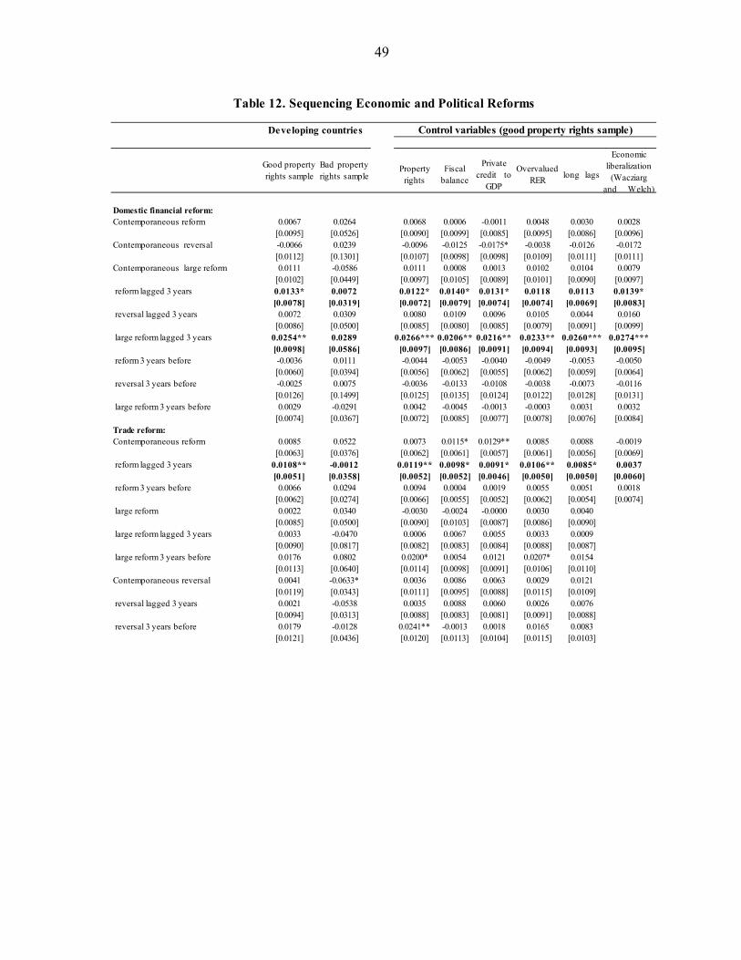
49

Property rights

Fiscal balance

Private credit to

GDP

Overvalued RER

long lags

Domestic financial reform:Contemporaneous reform 0.0067 0.0264 0.0068 0.0006 -0.0011 0.0048 0.0030 0.0028

[0.0095] [0.0526] [0.0090] [0.0099] [0.0085] [0.0095] [0.0086] [0.0096]Contemporaneous reversal -0.0066 0.0239 -0.0096 -0.0125 -0.0175* -0.0038 -0.0126 -0.0172

[0.0112] [0.1301] [0.0107] [0.0098] [0.0098] [0.0109] [0.0111] [0.0111]Contemporaneous large reform 0.0111 -0.0586 0.0111 0.0008 0.0013 0.0102 0.0104 0.0079

[0.0102] [0.0449] [0.0097] [0.0105] [0.0089] [0.0101] [0.0090] [0.0097] reform lagged 3 years 0.0133* 0.0072 0.0122* 0.0140* 0.0131* 0.0118 0.0113 0.0139*

[0.0078] [0.0319] [0.0072] [0.0079] [0.0074] [0.0074] [0.0069] [0.0083] reversal lagged 3 years 0.0072 0.0309 0.0080 0.0109 0.0096 0.0105 0.0044 0.0160

[0.0086] [0.0500] [0.0085] [0.0080] [0.0085] [0.0079] [0.0091] [0.0099] large reform lagged 3 years 0.0254** 0.0289 0.0266*** 0.0206** 0.0216** 0.0233** 0.0260*** 0.0274***

[0.0098] [0.0586] [0.0097] [0.0086] [0.0091] [0.0094] [0.0093] [0.0095] reform 3 years before -0.0036 0.0111 -0.0044 -0.0053 -0.0040 -0.0049 -0.0053 -0.0050

[0.0060] [0.0394] [0.0056] [0.0062] [0.0055] [0.0062] [0.0059] [0.0064] reversal 3 years before -0.0025 0.0075 -0.0036 -0.0133 -0.0108 -0.0038 -0.0073 -0.0116

[0.0126] [0.1499] [0.0125] [0.0135] [0.0124] [0.0122] [0.0128] [0.0131] large reform 3 years before 0.0029 -0.0291 0.0042 -0.0045 -0.0013 -0.0003 0.0031 0.0032

[0.0074] [0.0367] [0.0072] [0.0085] [0.0077] [0.0078] [0.0076] [0.0084]Trade reform:Contemporaneous reform 0.0085 0.0522 0.0073 0.0115* 0.0129** 0.0085 0.0088 -0.0019

[0.0063] [0.0376] [0.0062] [0.0061] [0.0057] [0.0061] [0.0056] [0.0069] reform lagged 3 years 0.0108** -0.0012 0.0119** 0.0098* 0.0091* 0.0106** 0.0085* 0.0037

[0.0051] [0.0358] [0.0052] [0.0052] [0.0046] [0.0050] [0.0050] [0.0060] reform 3 years before 0.0066 0.0294 0.0094 0.0004 0.0019 0.0055 0.0051 0.0018

[0.0062] [0.0274] [0.0066] [0.0055] [0.0052] [0.0062] [0.0054] [0.0074] large reform 0.0022 0.0340 -0.0030 -0.0024 -0.0000 0.0030 0.0040

[0.0085] [0.0500] [0.0090] [0.0103] [0.0087] [0.0086] [0.0090] large reform lagged 3 years 0.0033 -0.0470 0.0006 0.0067 0.0055 0.0033 0.0009

[0.0090] [0.0817] [0.0082] [0.0083] [0.0084] [0.0088] [0.0087] large reform 3 years before 0.0176 0.0802 0.0200* 0.0054 0.0121 0.0207* 0.0154

[0.0113] [0.0640] [0.0114] [0.0098] [0.0091] [0.0106] [0.0110]Contemporaneous reversal 0.0041 -0.0633* 0.0036 0.0086 0.0063 0.0029 0.0121

[0.0119] [0.0343] [0.0111] [0.0095] [0.0088] [0.0115] [0.0109] reversal lagged 3 years 0.0021 -0.0538 0.0035 0.0088 0.0060 0.0026 0.0076

[0.0094] [0.0313] [0.0088] [0.0083] [0.0081] [0.0091] [0.0088] reversal 3 years before 0.0179 -0.0128 0.0241** -0.0013 0.0018 0.0165 0.0083

[0.0121] [0.0436] [0.0120] [0.0113] [0.0104] [0.0115] [0.0103]

Control variables (good property rights sample)

Table 12. Sequencing Economic and Political Reforms

Developing countries

Good property rights sample

Bad propertyrights sample

Economic liberalization

(Wacziarg and Welch)

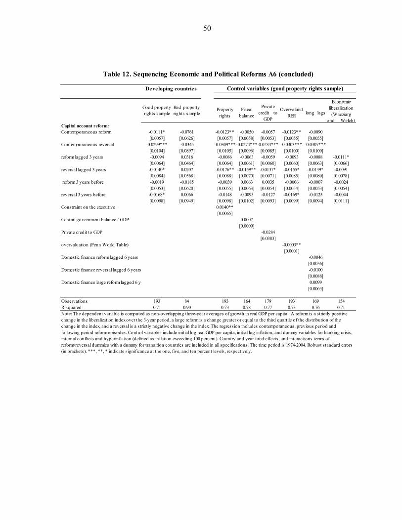
50

Property rights

Fiscal balance

Private credit to

GDP

Overvalued RER

long lags

Capital account reform:Contemporaneous reform -0.0111* -0.0761 -0.0123** -0.0050 -0.0057 -0.0123** -0.0090

[0.0057] [0.0626] [0.0057] [0.0058] [0.0053] [0.0055] [0.0055]Contemporaneous reversal -0.0299*** -0.0345 -0.0309***-0.0274***-0.0234*** -0.0303*** -0.0307***

[0.0104] [0.0897] [0.0105] [0.0096] [0.0085] [0.0100] [0.0100]reform lagged 3 years -0.0094 0.0316 -0.0086 -0.0063 -0.0059 -0.0093 -0.0088 -0.0111*

[0.0064] [0.0464] [0.0064] [0.0061] [0.0060] [0.0060] [0.0063] [0.0066]reversal lagged 3 years -0.0140* 0.0207 -0.0176** -0.0159** -0.0137* -0.0155* -0.0139* -0.0091

[0.0084] [0.0568] [0.0088] [0.0070] [0.0071] [0.0085] [0.0080] [0.0078] reform 3 years before -0.0019 -0.0185 -0.0039 0.0063 0.0035 -0.0006 -0.0007 -0.0024

[0.0053] [0.0620] [0.0055] [0.0063] [0.0054] [0.0054] [0.0053] [0.0054]reversal 3 years before -0.0168* 0.0066 -0.0148 -0.0093 -0.0127 -0.0169* -0.0125 -0.0044

[0.0098] [0.0949] [0.0098] [0.0102] [0.0093] [0.0099] [0.0094] [0.0111]Constraint on the executive 0.0140**

[0.0065]Central government balance / GDP 0.0007

[0.0009]Private credit to GDP -0.0284

[0.0383]overvaluation (Penn World Table) -0.0003**

[0.0001]Domestic finance reform lagged 6 years -0.0046

[0.0056]Domestic finance reversal lagged 6 years -0.0100

[0.0088]Domestic finance large reform lagged 6 y 0.0099

[0.0065]

Observations 193 84 193 164 179 193 169 154R-squared 0.71 0.90 0.73 0.78 0.77 0.73 0.76 0.71

Good property rights sample

Bad propertyrights sample

Economic liberalization

(Wacziarg and Welch)

Note: The dependent variable is computed as non-overlapping three-year averages of growth in real GDP per capita. A reform is a strictly positive change in the liberalization index over the 3-year period, a large reform is a change greater or equal to the third quartile of the distribution of the change in the index, and a reversal is a strictly negative change in the index. The regression includes contemporaneous, previous period and following period reform episodes. Control variables include initial log real GDP per capita, initial log inflation, and dummy variables for banking crisis, internal conflicts and hyperinflation (defined as inflation exceeding 100 percent). Country and year fixed effects, and interactions terms of reform/reversal dummies with a dummy for transition countries are included in all specifications. The time period is 1974-2004. Robust standard errors (in brackets). ***, **, * indicate significance at the one, five, and ten percent levels, respectively.

Table 12. Sequencing Economic and Political Reforms A6 (concluded)

Developing countries Control variables (good property rights sample)

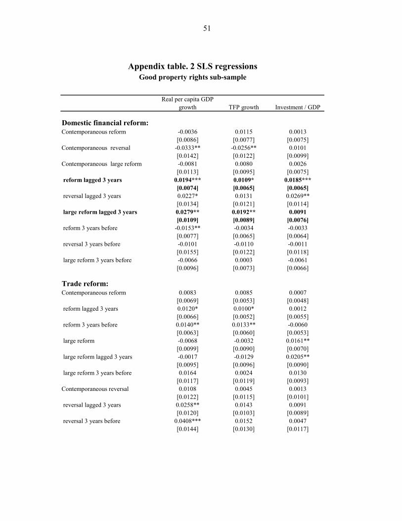
51

 

TFP growth

Domestic financial reform:Contemporaneous reform -0.0036 0.0115 0.0013

[0.0086] [0.0077] [0.0075]Contemporaneous reversal -0.0333** -0.0256** 0.0101

[0.0142] [0.0122] [0.0099]Contemporaneous large reform -0.0081 0.0080 0.0026

[0.0113] [0.0095] [0.0075] reform lagged 3 years 0.0194*** 0.0109* 0.0185***

[0.0074] [0.0065] [0.0065] reversal lagged 3 years 0.0227* 0.0131 0.0269**

[0.0134] [0.0121] [0.0114] large reform lagged 3 years 0.0279** 0.0192** 0.0091

[0.0109] [0.0089] [0.0076] reform 3 years before -0.0153** -0.0034 -0.0033

[0.0077] [0.0065] [0.0064] reversal 3 years before -0.0101 -0.0110 -0.0011

[0.0155] [0.0122] [0.0118] large reform 3 years before -0.0066 0.0003 -0.0061

[0.0096] [0.0073] [0.0066]

Trade reform:Contemporaneous reform 0.0083 0.0085 0.0007

[0.0069] [0.0053] [0.0048] reform lagged 3 years 0.0120* 0.0100* 0.0012

[0.0066] [0.0052] [0.0055] reform 3 years before 0.0140** 0.0133** -0.0060

[0.0063] [0.0060] [0.0053] large reform -0.0068 -0.0032 0.0161**

[0.0099] [0.0090] [0.0070] large reform lagged 3 years -0.0017 -0.0129 0.0205**

[0.0095] [0.0096] [0.0090] large reform 3 years before 0.0164 0.0024 0.0130

[0.0117] [0.0119] [0.0093]Contemporaneous reversal 0.0108 0.0045 0.0013

[0.0122] [0.0115] [0.0101] reversal lagged 3 years 0.0258** 0.0143 0.0091

[0.0120] [0.0103] [0.0089] reversal 3 years before 0.0408*** 0.0152 0.0047

[0.0144] [0.0130] [0.0117]

Real per capita GDP growth Investment / GDP

Appendix table. 2 SLS regressionsGood property rights sub-sample

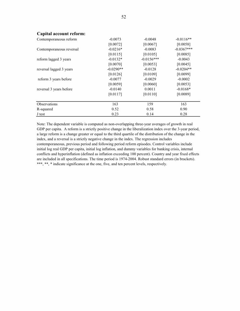
52

 Capital account reform:Contemporaneous reform -0.0073 -0.0048 -0.0116**

[0.0072] [0.0067] [0.0058]Contemporaneous reversal -0.0216* -0.0083 -0.0367***

[0.0115] [0.0105] [0.0085]reform lagged 3 years -0.0132* -0.0156*** -0.0043

[0.0070] [0.0053] [0.0045]reversal lagged 3 years -0.0290** -0.0128 -0.0204**

[0.0126] [0.0109] [0.0099] reform 3 years before -0.0077 -0.0029 -0.0002

[0.0059] [0.0060] [0.0053]reversal 3 years before -0.0140 0.0011 -0.0168*

[0.0117] [0.0110] [0.0089]

Observations 163 159 163R-squared 0.52 0.58 0.90J test 0.23 0.14 0.28

Note: The dependent variable is computed as non-overlapping three-year averages of growth in real GDP per capita. A reform is a strictly positive change in the liberalization index over the 3-year period, a large reform is a change greater or equal to the third quartile of the distribution of the change in the index, and a reversal is a strictly negative change in the index. The regression includes contemporaneous, previous period and following period reform episodes. Control variables include initial log real GDP per capita, initial log inflation, and dummy variables for banking crisis, internal conflicts and hyperinflation (defined as inflation exceeding 100 percent). Country and year fixed effects are included in all specifications. The time period is 1974-2004. Robust standard errors (in brackets). ***, **, * indicate significance at the one, five, and ten percent levels, respectively.