Policy Research Working Paper 6842

Growth, Inequality, and Social Welfare

Cross-Country Evidence

David DollarTatjana Kleineberg

Aart Kraay

The World BankDevelopment Research GroupMacroeconomics and Growth TeamApril 2014

WPS6842P

ublic

Dis

clos

ure

Aut

horiz

edP

ublic

Dis

clos

ure

Aut

horiz

edP

ublic

Dis

clos

ure

Aut

horiz

edP

ublic

Dis

clos

ure

Aut

horiz

edP

ublic

Dis

clos

ure

Aut

horiz

edP

ublic

Dis

clos

ure

Aut

horiz

edP

ublic

Dis

clos

ure

Aut

horiz

edP

ublic

Dis

clos

ure

Aut

horiz

ed

Produced by the Research Support Team

Abstract

The Policy Research Working Paper Series disseminates the findings of work in progress to encourage the exchange of ideas about development issues. An objective of the series is to get the findings out quickly, even if the presentations are less than fully polished. The papers carry the names of the authors and should be cited accordingly. The findings, interpretations, and conclusions expressed in this paper are entirely those of the authors. They do not necessarily represent the views of the International Bank for Reconstruction and Development/World Bank and its affiliated organizations, or those of the Executive Directors of the World Bank or the governments they represent.

Policy Research Working Paper 6842

Social welfare functions that assign weights to individuals based on their income levels can be used to document the relative importance of growth and inequality changes for changes in social welfare. In a large panel of industrial and developing countries over the past 40 years, most of the cross-country and over-time variation in changes

This paper is a product of the Macroeconomics and Growth Team, Development Research Group. It is part of a larger effort by the World Bank to provide open access to its research and make a contribution to development policy discussions around the world. Policy Research Working Papers are also posted on the Web at http://econ.worldbank.org. The authors may be contacted at akraay@worldbank.org.

in social welfare is due to changes in average incomes. In contrast, the changes in inequality observed during this period are on average much smaller than changes in average incomes, are uncorrelated with changes in average incomes, and have contributed relatively little to changes in social welfare.

Growth, Inequality, and Social Welfare: Cross-Country Evidence

David Dollar (Brookings) Tatjana Kleineberg (Yale) Aart Kraay (World Bank)

Keywords: growth, inequality

JEL Classification Codes: O4, O11, I3

ddollar@brookings.edu, tatjana.kleineberg@yale.edu, akraay@worldbank.org. This paper is being prepared for Economic Policy. We would like to thank, without implication, David Bulman, Pete Lanjouw and Luis Serven for helpful comments. Financial support from the Knowledge for Change Program of the World Bank is gratefully acknowledged. The views expressed here are the authors' and do not reflect those of the Brookings Institution, the World Bank, its Executive Directors, or the countries they represent.

1. Introduction

Concerns about inequality are at the forefront of many policy debates today. From the “we are

the 99 percent” slogans of the Occupy Wall Street movement, to major policy speeches by US President

Barack Obama, it is hard to escape the view that rising inequality poses major challenges in advanced

economies. In the developing world too, much has been written about the adverse effects of high and

rising inequality on the pace of absolute poverty reduction. Concerns about inequality appear to be

pervasive beyond policy elites as well. Public opinion surveys suggest that strong majorities of

respondents in advanced economies feel that the gap between rich and poor has been rising in recent

years. According to a recent Pew survey, over 80 percent of respondents in advanced economies are of

the view that the gap between rich and poor has been increasing.1

These views no doubt in part reflect the fact that inequality has in fact been increasing in many

countries. In the US over the past four decades, the Gini coefficient has risen from around 30 to around

40. Roughly the same has happened in China, only more rapidly: between 1990 and 2009 the Gini

coefficient has increased from 32 to 42. Much of this increase has happened at the upper end of the

income distribution. According to Atkinson, Piketty and Saez (2011), the income share of the top 10

percent in the US has increased from around 33 percent in 1970 to nearly 50 percent in 2007, while in

China it increased from 17 to 28 percent between 1986 and 2003.

However, it is also important not to lose sight of the fact that inequality has not increased in

other countries, and has declined appreciably in still others. In the Atkinson, Piketty and Saez (2011)

data, income shares of the top decile have been stable or even declining slightly since the mid-20th

century in countries such as Germany, France, Switzerland, and the Netherlands. In Brazil, the Gini

coefficient has declined from around 60 in the late 1990s to around 55 in the late 2000s. More

systematically, in a large dataset of changes in inequality over periods at least five years long that we

describe in more detail below, in roughly half of episodes the Gini coefficient of inequality increases,

while in the other half of episodes it decreases.

In this paper, we aim to shed light on a very simple question: how much do these changes in

inequality, in either direction, matter? To answer this question we first need to be precise about what

we mean by “matter”. Our approach here is unabashedly modest: we use standard tools of social

welfare analysis to calculate how much more or less growth in average incomes a country would need

1 See Pew Research Center (2013)

2

over a given period in order to compensate for the observed change in inequality over the same period.

We then document the size of this compensation, and its relationship to average income growth, in a

large dataset of episodes of growth and changes in inequality covering 117 countries between 1970 and

2012.

A simple example helps to illustrate our approach. The World Bank has recently made a major

public commitment to the goal of promoting “shared prosperity”, defined as growth in average incomes

of those in the bottom 40 percent of the income distribution in each country in the developing world.2

As a matter of simple arithmetic, growth in average incomes in the bottom 40 percent is the sum of

growth in average incomes, and growth in the share of income accruing to the bottom 40 percent. In

China, for example, between 1990 and 2009 average incomes grew at 6.7 percent per year. At the same

time, inequality increased in the sense that the income share of the bottom 40 percent declined from

20.2 percent to 14.4 percent, corresponding to an average annual rate of -1.7 percent per year.

Combining these two observations, average incomes in the bottom 40 percent grew more slowly than

overall average income, at 5 percent per year. From the standpoint of promoting shared prosperity,

therefore, the growth “cost” of the increase in inequality in China over this period is about 1.7

percentage points of growth per year. Or put differently, had inequality not increased in China during

this time, a growth rate of 5 percent per year (instead of the 6.7 percent that actually happened) would

have generated the same improvement in social welfare according to the “shared prosperity” metric of

the World Bank.

This example illustrates the two key ingredients in our approach. First, in order to understand

how much inequality changes “matter”, we need to specify a social welfare function that assigns weights

to individuals in a country based on their incomes. In the case of the World Bank’s “shared prosperity”

target, the implicit social welfare function weights everyone in the bottom 40 percent of the income

distribution in proportion to their incomes, and assigns zero weight to everyone in the upper 60 percent

of the income distribution. In our empirical work, we will consider a variety of very standard social

welfare functions corresponding to different preferences over how income is distributed across

individuals in a country. Second, growth in social welfare between two points in time will reflect growth

in average incomes, and growth in the relevant inequality measure implied by the particular social

welfare function under consideration. In the case of the World Bank’s “shared prosperity” target, the

relevant inequality measure is the income share of the bottom 40 percent. For all of the social welfare

2 See World Bank (2013).

3

functions we consider, this decomposition will be additive, allowing for a straightforward quantification

of the relative importance of growth and inequality changes, and the costs or benefits in terms of

growth of the latter. In particular, the increase (decrease) in the relevant inequality measure in

percentage points per year can be interpreted as the amount by which average income growth would

have to be higher (lower) to deliver the observed growth rate of social welfare absent any changes in

income distribution.

We work with a large dataset of income distributions and average incomes covering 117

countries over the past four decades. This dataset combines the high-quality household survey data for

developing countries underlying the World Bank’s global poverty estimates (Ravallion and Chen (2010)),

with the Luxembourg Income Study (LIS) data for advanced economies. We focus on within-country

changes in average incomes and income inequality observed over episodes at least five years long. In a

sample of 285 such non-overlapping episodes, we calculate the contribution of growth in average

incomes, and the contribution of changes in inequality, to growth in social welfare, for a wide variety of

social welfare functions.

Our basic findings are easily summarized. For all of the social welfare functions we consider,

social welfare on average increases equiproportionately with average incomes. This reflects the fact that

changes in the relevant inequality measures are not systematically correlated with changes in average

incomes. For all but the most bottom-sensitive social welfare functions, the relationship between

growth in social welfare and growth in average incomes is also quite precisely estimated. This reflects

the fact that changes in inequality are small, in the sense that variation across episodes in inequality

accounts for only a small fraction of the variation across episodes in changes in social welfare.

Although changes in social welfare driven by changes in the relevant inequality measures are on

average small and uncorrelated with growth in average incomes, it is nevertheless useful to understand

their correlates. In particular, if there were some combination of policies and institutions that

supported a given growth rate of overall per capita incomes, but in addition led to declines in the

relevant inequality measure, then from the standpoint of promoting social welfare, such policies would

dominate others that did not lead to the same declines in inequality. In the last part of the paper, we

consider a range of variables identified as important for growth and inequality in the large empirical

cross-country literature. In the spirit of comprehensive data description, we use Bayesian Model

Averaging to systematically document the partial correlations between these variables and growth in

average incomes and in inequality, and through these channels, their correlations with social welfare.

4

We find little in the way of compelling empirical evidence that any of these variables are robustly

correlated with the relevant changes in inequality that matter for the set of social welfare functions that

we consider.

This paper builds on our previous work in Dollar and Kraay (2002) and Dollar, Kleineberg and

Kraay (2013). In those papers we studied the relationship between growth in average incomes and

growth in average incomes in the bottom 20 percent and bottom 40 percent of the income distribution.

Our findings in this paper are generally consistent with this earlier work – in these papers we also found

that changes in the income share of the poorest quintiles typically are small and uncorrelated with

changes in average incomes. This paper expands on our earlier work by considering a much broader

class of social welfare functions, which allows us to connect our previous findings specific to the income

shares of the poorest quintiles with more general inequality measures. Our emphasis in this paper on

decomposing changes in social welfare into a growth component and a distribution component is

related to the large literature that has followed Datt and Ravallion (1992) in decomposing changes in

poverty measures into growth and distribution components (see Kraay (2006) for a recent application to

absolute poverty measures in a large cross-country dataset).

In Section 2 we describe the social welfare functions we study, and show how growth in social

welfare can be decomposed into growth and inequality changes. Section 3 briefly describes the data,

and Section 4 contains our main results on the relative importance of growth and inequality changes for

growth in social welfare. Section 5 uses Bayesian Model Averaging to systematically relate changes in

social welfare to a variety of policy variables that have been considered in the cross-country empirical

literature, and Section 6 concludes.

2. Growth, Changes in Inequality, and Social Welfare

We study the relationship between growth in average incomes and growth in social welfare.

Our starting point is a social welfare function which specifies the weights assigned to different groups in

a country. While in principle we could work with social welfare functions defined over individuals, in

practice data limitations imply that we only directly observe deciles of the income distribution in the

developing countries in our dataset. For this reason we consider social welfare functions that assign

5

weights to deciles rather than individuals. In addition, we consider only social welfare functions defined

over income.3

In particular we consider social welfare functions which assign weights to deciles of the income

distribution, indexed by 𝑖 = 1, … ,𝑁, based on average income in these deciles:

(1) W = 𝐹(𝑌1, … ,𝑌𝑁)

where 𝑌𝑖 denotes average income in decile 𝑖, with higher values of 𝑖 corresponding to richer deciles, i.e.,

𝑌1 < 𝑌2 < ⋯ < 𝑌𝑁. We will consider three well-known cases of this social welfare function. The first

equally weights incomes in selected deciles, and assigns zero weight to incomes in the remaining deciles,

i.e.

(2) W = �𝐷𝑖𝑌𝑖

∑ 𝐷𝑗𝑁𝑗=1

𝑁

𝑖=1

where 𝐷𝑖 = 1 if decile 𝑖 matters for the social welfare function in question, and zero otherwise. For

example, the World Bank’s shared prosperity goal mentioned in the introduction implies a social welfare

function where 𝐷1 = 𝐷2 = 𝐷3 = 𝐷4 = 1 and zero otherwise, i.e. average incomes in the bottom 40

percent of the income distribution. As another example, the work of Piketty and Saez focusing on how

incomes in the top decile have diverged from those in the remaining 90 percent of the income

distribution can be interpreted through the lens of this social welfare function with 𝐷1 = 𝐷2 = ⋯ =

𝐷9 = 1 and 𝐷10 = 0, i.e average incomes in the bottom 90 percent of the income distribution.

The second is a social welfare function proposed by Sen (1976), which weights the income of

each group by its rank in the income distribution:

3 More generally, one could consider social welfare functions that reflect the lifetime utility of individuals, which in turn depends on present and future consumption, labour supply, and longevity, among many other things. See for example Jones and Klenow (2011), Basu et al (2013) for cross-country applications in a representative agent setting, and Perri and Krueger (2003) for an individual-level application in the US.

6

(3) W =2𝑁2�(𝑁 + 1 − 𝑖)𝑌𝑖

𝑁

𝑖=1

In contrast with the “selected deciles” approach, this social welfare function assigns positive weight to

all deciles, and not just the poorest. However, in contrast with simple average income, this social

welfare function is pro-poor in the sense that it places more weight on the incomes of poorer groups:

the weight placed on incomes in the poorest decile (𝑖 = 1) is ten times the weight placed on incomes in

the richest decile (𝑖 = 10). When the number of groups 𝑁 is large, Sen (1976) shows that 𝑊 =

𝜇(1 − 𝐺), where 𝜇 represents average income and 𝐺 represents the Gini coefficient. This formulation

will be particularly useful because it makes it very straightforward to interpret the magnitude of changes

in (one minus) the Gini coefficient in terms of growth in average incomes.

The third social welfare function is the class proposed by Atkinson (1970):

(4) W = �1𝑁�𝑌𝑖1−𝜃𝑁

𝑖=1

�

11−𝜃

for 𝜃 ≥ 0 and 𝜃 ≠ 1 (for 𝜃 = 1 this limits to a geometric average of incomes, 𝑊 = �∏ 𝑌𝑖𝑁𝑖=1 �1/𝑁

). To

interpret this social welfare function, note that 𝑊1−𝜃 is a weighted average of the incomes of each

decile, with weights proportional to 𝑌𝑖−𝜃. When 𝜃 = 0, the income weights are equal and the social

welfare function collapses to average income. As 𝜃 becomes larger, the social welfare function assigns

greater weight to the incomes of the poorest groups. This social welfare function can also be written as

the product of a particular inequality measure and average incomes, i.e. 𝑊 = 𝜇(1 − 𝐴), where 𝐴

denotes the Atkinson inequality index 𝐴 ≡ 1 − 1𝜇�1𝑁∑ 𝑌𝑖1−𝜃𝑁𝑖=1 �

11−𝜃.

Figure 1 provides a graphical summary of these different social welfare functions. The top panel

depicts the weights assigned to incomes of different percentiles of the income distribution, normalized

to sum to one for each social welfare function. All of the social welfare functions are (weakly)

downward sloping, reflecting the fact that they assign greater weight to lower incomes. As noted

above, average incomes in the bottom 40 percent equally weights incomes in the bottom 40 percent but

gives zero weight to incomes above this threshold. The Sen index weights incomes in proportion to

ranks in the income distribution, and so is a straight downward-sloping line. Relative to the Sen index,

the A(1) and A(2) measures assign even more weight to the poorest percentiles. Finally, we also show

A(0) which is simply average incomes – this naturally weights incomes of all percentiles equally.

7

The bottom panel of Figure 1 shows the weights assigned to individuals in each percentile of the

income distribution, in contrast with the weights assigned to their incomes in the top panel (again we

normalize the weights to sum to one across percentiles). Consider first average incomes, as captured by

A(0). Since average income weights all incomes equally, it assigns less weight to poor people and more

weight to rich people, with weights proportional to relative incomes. The same is true within the

bottom 40 percent of the income distribution for the social welfare function corresponding to “shared

prosperity” – it assigns greatest weight to individuals at the 40th percentile of the income distribution,

and lower weights to poorer people within the bottom 40 percent. This same non-monotonic set of

weights on individuals is implied by the Sen index, which gives greatest weight to individuals near the

middle of the income distribution, and low weights to those at the lower and upper extremes of the

distribution. The A(1) measure is an interesting benchmark because it weights all individuals equally.

For values of 𝜃 > 1, the Atkinson index assigns greater weight to poorer individuals.

The main benefit of specifying an explicit social welfare function is that it allows us to quantify

the contributions of growth in average incomes and changes in inequality to changes in overall social

welfare. For the social welfare functions we consider, growth in social welfare is given by:

(5) 𝑑𝑊𝑊

= �𝜀𝑖𝑑𝑌𝑖𝑌𝑖

𝑁

𝑖=1

where 𝜀𝑖 = 𝜕𝐹𝜕𝑌𝑖

𝑌𝑖𝐹

is the elasticity of the social welfare function with respect to group 𝑖’s income. In

order to distinguish between changes in average incomes and changes in relative incomes, it is useful to

decompose income growth within each decile into average income growth plus the share of income

accruing to that decile, i.e. 𝑑𝑌𝑖𝑌𝑖

= 𝑑𝜇𝜇

+ 𝑑𝑠𝑖𝑠𝑖

, where 𝜇 denotes average income and 𝑠𝑖 denotes the income

share of decile 𝑖. Using this, combined with the fact that the social welfare functions we consider are all

homogenous of degree one, i.e. ∑ 𝜀𝑖𝑁𝑖=1 = 1, gives the following decomposition of growth in social

welfare into growth in average incomes and a weighted average of changes in relative incomes.4

4 The Sen index is homogenous of degree one only in the limit as N goes to infinity. By focusing on social welfare functions that are homogenous of degree one we are ruling out absolute inequality measures such as the Kolm

8

(6) 𝑑𝑊𝑊

=𝑑𝜇𝜇

+�𝜀𝑖𝑑𝑠𝑖𝑠𝑖

𝑁

𝑖=1

Depending on the choice of SWF, this expression tells us how to weight changes in inequality happening

at different parts of the income distribution, i.e. changes in the income shares of different

individuals/groups within the population. In particular, (i) for the “selected deciles” social welfare

functions, the weights are 𝜀𝑖 = 𝐷𝑖𝑌𝑖∑ 𝐷𝑗𝑌𝑗𝑁𝑗=1

; (ii) for the Sen index the weights are 𝜀𝑖 = (𝑁+1−𝑖)𝑌𝑖∑ (𝑁+1−𝑗)𝑌𝑗𝑁𝑗=1

; and

(iii) for the Atkinson index the weights are 𝜀𝑖 = 𝑌𝑖1−𝜃

�∑ 𝑌𝑗1−𝜃𝑁𝑗=1 �

. These weights on changes in income shares

of different percentiles of the income distribution are exactly those shown in the bottom panel of Figure

1.

This additive decomposition of welfare changes into growth in average incomes and a weighted

average of changes in income shares allows a natural interpretation of changes in inequality in terms of

growth. In particular, the second term in Equation (6) is just the difference between growth in welfare

and growth in average incomes, and it can be interpreted as the “growth cost” of the observed increase

in inequality, i.e. the amount by which growth would have to be higher in order to compensate for the

increase in inequality, in the sense of delivering the same welfare growth. In the remainder of this

paper we implement and analyze this decomposition in a large dataset of cross-country dataset of

income distributions over the past forty years.

3. Data

Our starting point is a large dataset of 963 irregularly-spaced country-year observations for

which household surveys are available, covering a total of 151 countries between 1967 and 2011. This

dataset is the merger of data available in two high-quality compilations of household survey data: the

World Bank’s POVCALNET database, covering primarily developing countries, and the Luxembourg

Income Study (LIS) database, covering primarily developed countries. The POVCALNET database is the

dataset underlying the World Bank's widely known global poverty estimates. Its data on average

index, as well as absolute poverty measures such as the headcount or the poverty gap. For such measures, decompositions such as the one suggested in Datt and Ravallion (1992) are more appropriate.

9

incomes and income distribution are based on primary household survey data. Roughly half of the

surveys in the POVCALNET database report income and its distribution, while the other half report

consumption expenditure and its distribution. When we study within-country changes in the

distribution of income or consumption, we focus only on episodes where the initial and final survey are

of the same type, i.e. both refer to income or both refer to expenditure. For terminological

convenience, however, we will refer only to income. All survey means are expressed in constant 2005

US dollars adjusted for differences in purchasing power parity.

For countries that are not covered in POVCALNET, we rely on the LIS database.5 This expands

our sample by adding 19 OECD economies. For these countries we construct mean income and decile

shares directly from the micro data at the household level. The underlying surveys are nationally

representative and intended to be comparable over time. We focus on the LIS measure of household

total income, which is expressed in the raw data in current local currency units. We convert the survey

means to constant 2005 USD and then apply the 2005 purchasing power parity for consumption from

the Penn World Table, in order to be consistent with the POVCALNET data. Also for consistency with the

POVCALNET data, we use LIS data on household size and equivalence scales to convert to average

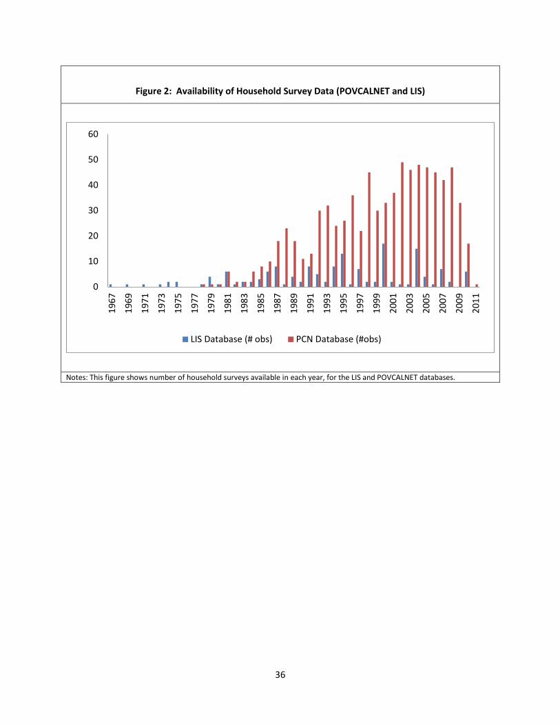
income and its distribution across individuals rather than households. Figure 2 gives an overview of the

annual data availability from these two sources. LIS survey data starts earlier, going back to 1967, while

POVCALNET observations start in the 1980s. Both databases have better country coverage in more

recent years.

For our empirical analysis, we organize the data into episodes or “spells”, defined as within-

country changes in variables of interest between two survey years. Specifically, we calculate the

average annual log differences of social welfare and its components, average annual growth in mean

income and in the relevant inequality measures for each spell, recognizing that different spells cover

periods of different length, depending on the availability of household survey data. We work with two

sets of spells corresponding to different time horizons. The first is the longest available spell for each

country, i.e. from the first available to the most recently-available survey for each country, while the

second is the set of all possible consecutive non-overlapping spells lasting at least five years, beginning

with the first available survey for each country. We can only compute these spells for countries where

at least two comparable surveys separated by at least 5 years are available.

5 A handful of countries have surveys available both through POVCALNET and LIS. For these countries we use only the POVCALNET data, i.e. we do not switch within countries between POVCALNET and LIS.

10

While the data we rely on come from the most reliable cross-country datasets on income

distribution currently available, there nevertheless are some spells where the changes in average

income and/or changes in decile shares over the spell are extreme. To prevent these from unduly

influencing our results, we clean the data by truncating the sample at the first and 99th percentiles of the

distribution of average growth and of each of the 10 decile shares. This leaves us with a final sample

consisting of 117 countries, with a median length between the first and last available surveys of 16

years. For the sample of spells at least five years long, we have a total of 285 spells, with a median spell

length of 6 years.

4. Results

4.1 Basic Description

We begin with some very simple descriptive analysis of the relative importance of growth and

changes in inequality for growth in social welfare. The eight panels of Figure 3 plot growth in social

welfare (on the vertical axis) against growth in average incomes (on the horizontal axis) in the sample of

minimum 5-year long spells, for eight measures of social welfare: average incomes in the bottom 10, 20,

40 and 90 percent of the income distribution, the Sen index, and the Atkinson index with values of 𝜃

equal to 1, 2 and 3. Since growth in social welfare is the sum of growth in average incomes and the

growth rate in the relevant inequality measure, the vertical distance between each point and the 45

degree line reflects the contribution of inequality changes to growth in social welfare. The striking

feature of these graphs is that, for most social welfare functions, the data points cluster very closely

around the 45-degree line. This indicates that changes in social welfare due to inequality changes (in

either direction) are small, particularly in comparison with the large variation in growth rates in average

incomes apparent on the horizontal axis of each graph. Only in the case of very bottom-sensitive social

welfare functions that place a very high weight on the poorest deciles (such as average incomes in the

bottom 10 percent, or the Atkinson A(3) measure), do we begin to see more dispersion around the 45-

degree line.

Figure 4 provides a complementary perspective on the relative size of changes in growth and

changes in inequality. We first plot the distribution of growth rates across all episodes in our sample of

spells at least five years long. This distribution has a mean of 1.5 percent per year, and very substantial

variation: the standard deviation of growth in average incomes is 4.2 percent, and the 10th and 90th

percentiles of the distribution of growth in average incomes are -2.8 percent and 6.2 percent

11

respectively. In short, growth in mean income is positive on average, and exhibits very large variation

across spells.

We then superimpose the distribution of growth rates of inequality changes in the same sample,

for each of the eight social welfare functions we consider. The contrast between the distribution of

growth rates and the distribution of inequality changes is stark. Consider for example the Sen Index,

where the relevant inequality measure is (one minus) the Gini index. The mean growth rate of this

inequality measure is very close to zero, at 0.0 percent per year. There is also substantially less variation

across spells in changes in inequality than there is in growth: the standard deviation of changes in

inequality for the Sen index is 1.2 percent, and the 10th and 90th percentiles of the distribution of

inequality changes are -1.5 percent and 1.7 percent respectively.

A useful thought experiment here is to ask the following question: from the perspective of

having rapid expected growth in social welfare, would we prefer to take a random draw from the

distribution of average income growth or a random draw from the distribution of inequality changes? If

our social welfare function is the Sen index, the answer is unambiguously to prefer a draw from the

distribution of growth rates. As noted above, the mean of the distribution of growth rates is 1.5 percent

per year, while for inequality changes it is essentially zero. Even if we were to get a very good draw

from the distribution of inequality changes (say at the 90th percentile), this would deliver a growth rate

of social welfare only slightly faster than what we could get at the average of the distribution of mean

income growth (1.7 versus 1.5 percent per year).

These results on the relative importance of growth hold roughly the same for most of the social

welfare functions we consider, with the exception of the most bottom-sensitive ones, average incomes

in the bottom 10 percent, and the Atkinson A(3) index. For these social welfare functions, we continue

to find that the distribution of the relevant inequality changes is centered on roughly zero: the average

change in inequality across spells is 0.2 percent per year. However, changes in inequality exhibit

considerably more variation. For example, for the Atkinson A(3) index the standard deviation of

inequality changes is 4 percent, which is quite close to that for growth in average incomes.

Table 1 reports summary statistics on the distributions of growth rates and inequality changes

more systematically, and for different subsamples. The first column refers to average income growth,

while the remaining eight columns correspond to growth in the relevant inequality measure for each of

the eight social welfare functions we consider. Each horizontal panel corresponds to a different sample

12

of observations, and within each panel we report the number of observations, the mean, the standard

deviation, and the 10th and 90th percentiles of the distribution of growth rates within each sample. The

first panel reports summary statistics for the sample of long spells, and the sample of minimum-five-

year spells. The second panel disaggregates the minimum-five-year spell sample into low-income,

middle-income, and high-income countries. The third panel disaggregates the minimum-five-year spells

by decades.6

The summary statistics in the first panel reflect the previous discussion on the mean and relative

variability of changes in average incomes and changes in inequality. Looking across income categories in

the second panel, we see that growth on average was substantially higher in the low-income country

spells (2.5 percent per year versus 1.3 percent per year in the middle- and high-income categories).

Across all the different social welfare functions, however, we still see that growth in the relevant

inequality measure was on average close to zero in all three income categories. Looking across decades,

we see clear evidence of an acceleration in average growth rates of survey mean income, from near zero

in the 1980s and 1990s to 2.8 percent per year in the 2000s. There was however little change in the

growth rate of any of the inequality measures across decades, with the implication that average growth

in social welfare increased by roughly as much as growth in average incomes increased.

4.2 Regression Analysis

We next shed light on the joint distribution of growth rates and inequality changes, using a

series of simple ordinary least squares regressions of growth in social welfare on growth in average

incomes. Since the former is the sum of growth in average incomes and changes in the relevant

inequality measure, the slope coefficient from this regression is:

(7) 1 + COV�𝑑𝜇𝜇

,�𝜀𝑖𝑑𝑠𝑖𝑠𝑖

𝑁

𝑖=1

� /𝑉𝐴𝑅 �𝑑𝜇𝜇�

6 A practical challenge for data description here is that only a small fraction of spells fall entirely within a single decade, and so it is not obvious how to assign the remaining spells to decades. To circumvent this problem, for each spell we define three variables measuring the fraction of years in the spell falling in each of three decades. For example, a spell lasting from 1989 to 1994 would have one-fifth of its years in the 1980s and four-fifths in the 1990s, and none in the 2000s. We then report weighted summary statistics by decade, weighting each spell by the fraction of observations falling in each decade.

13

i.e. it is 1 plus the slope coefficient of a regression of changes in inequality on growth. If the estimated

slope coefficient is equal to one, this implies that on average, social welfare increases

equiproportionately with average incomes. If, on the other hand, the slope coefficient is greater (less)

than one, social welfare increases more (less) than equiproportionately with average incomes, reflecting

a decline (increase) in the relevant inequality measure when average incomes increase.

In addition, the goodness of fit of these regressions is informative about the relative importance

of growth and inequality changes for growth in social welfare. In particular, it is straightforward to show

that the share of the variance in growth in social welfare due to growth in average incomes is:

(8) 𝑅 SD �𝑑𝜇𝜇� /SD �

𝑑𝑊𝑊

�

where 𝑅 is the square root of the R-squared from a regression of growth in social welfare on growth in

average incomes and 𝑆𝐷(𝑥) denotes the standard deviation of 𝑥.7

The top (bottom) panels of Table 2 report these regressions for the sample of spells at least five-

years long (for the sample of long spells). As before, the eight columns correspond to the eight social

welfare functions we consider. The regressions confirm the visual impressions from Figure 3 as the

estimated slopes are all very close to one. In all cases we cannot reject (at the 5 percent significance

level) the null hypothesis that the estimated slope coefficient is equal to one, indicating an absence of

any statistically significant correlation between changes in average income and changes in inequality

that are relevant for the social welfare measures we consider. One interesting exception is the slope for

the income of the bottom 10%, which is 1.15 with a standard error of 0.08 in the sample of minimum-

five-year spells, and is significantly greater than one at the 9 percent significance level. This constitutes

some weak evidence that the income share of the bottom decile does on average increase when

average incomes increase. However, we do not find this in the sample of long spells for this inequality

measure, or for any of the other inequality measures.

Turning to the variance decompositions, we see that, for most social welfare functions, most of

the variation in growth in social welfare is due to growth in average incomes. For example, for the Sen

Index and the income share of the bottom 40 percent, the shares of the variance of growth in social

welfare due to growth in average incomes are 92 and 77 percent in the minimum-five-year spells. As we

7 We follow Klenow and Rodriguez-Clare (1997) in defining the share of the variance of 𝑋 + 𝑌 due to 𝑋 as (𝑉(𝑋) + 𝐶𝑂𝑉(𝑋,𝑌)/𝑉(𝑋 + 𝑌). Since the correlation between growth and inequality changes is small, the term 𝐶𝑂𝑉(𝑋,𝑌) plays a minimal role in the decompositions that follow.

14

move to measures that place more weight on the poorest deciles, this variance share declines further, to

60 percent for the bottom 20 percent measure, and 52 and 41 percent for the Atkinson A(3) and bottom

10 percent measures.

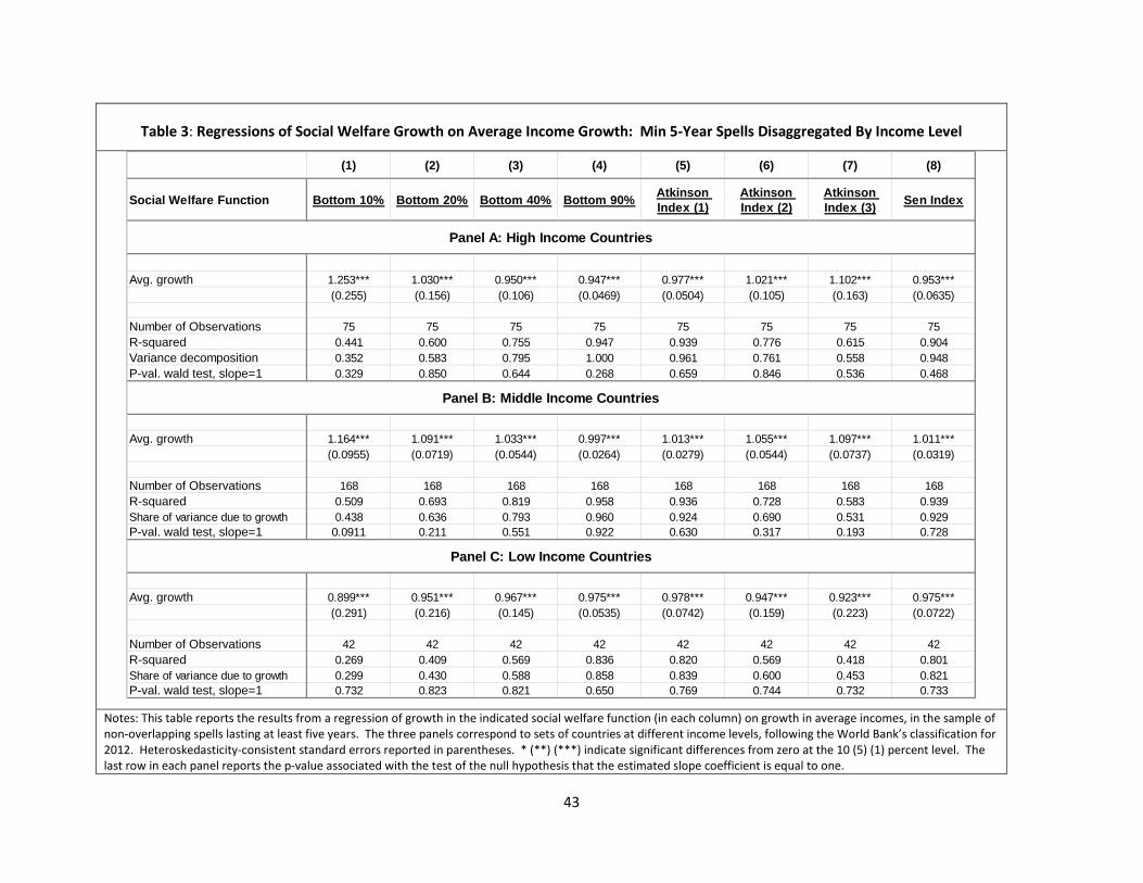
In Table 3, we disaggregate our results by income level, focusing on the sample of spells lasting

at least five years. The results are very similar for low-income, middle-income, and high-income

countries. In all but one case we cannot reject the hypothesis that the slope is 1.0. The one exception is

the social welfare function corresponding to income of the bottom 10 percent in middle-income

countries, where the slope is slightly greater than one, at 1.16, indicating a weak tendency for the

income share of the poorest 10 percent to rise as average incomes increase in this sample. We also

continue to see that the share of the variance of growth in social welfare due to growth in average

incomes is high, particularly for measures such as the Sen index and average incomes of the bottom 40

and 90 percent. This is particularly the case in high- and middle-income countries. In contrast, among

low-income countries we find that the share of the variance of growth in social welfare due to growth is

somewhat lower than in the middle- and high-income countries.

In Table 4, we disaggregate our results by decade, again focusing on the sample of spells at least

five years long. Across all periods and for all social welfare functions, we continue to find a slope

coefficient that is very close to, and not statistically significantly different from one, indicating an

absence of a significant relationship between changes in inequality and changes in average incomes.

One consistent pattern, however, is that the share of the variance of growth in social welfare due to

growth in average incomes declines slightly as we move from the 1980s to the 1990s to the 2000s. For

example, for the bottom 40 percent social welfare function, this variance share declines from 85 percent

in the 1980s to 72 percent in the 2000s.8

In all of our results so far, we have relied exclusively on household survey means to construct

growth rates in average incomes. A large literature has discussed substantial differences between

growth in survey mean income and corresponding aggregates in the national accounts in some countries

(see for example Deaton (2005) and Deaton and Kozel (2005) for the case of India in particular).

8 Interestingly, this decline in the variance share does not appear to be due to compositional effects (noticing that the sample size increases significantly over time). As a robustness check, we constructed a sample of 43 countries with one survey available near the middle of each of the three decades. We then constructed two sets of spells, from the mid-1980s to the mid-1990s, and from the mid-1990s to the mid-2000s. In this smaller set of spells we also find that the share of the variance of growth in social welfare due to growth in average incomes falls in the second set of spells relative to the first.

15

Without taking a stand on relative merits of national accounts versus household surveys as a measure of

average living standards, we perform some simple robustness checks to see how our findings change if

we rely on national accounts growth rates instead of household survey mean growth rates.

The results are shown in Table 5, again focusing on the sample of spells at least five years long.

Panel A repeats the results for all eight measures using the survey data. Panel B alternatively uses the

growth rate of real private consumption from the national accounts. The slopes all continue to be very

close to one. The main difference is that the share of welfare growth attributed to income growth

declines modestly when we move to national accounts data. For example, for A(1) that share is 92%

using the survey data; it declines to 85% using the alternative measure from the national accounts.

4.3 Why Is the Importance of Growth Different Across Social Welfare Functions?

One striking feature of our empirical results is that the role of growth in accounting for changes

in social welfare appears to be smaller for more bottom-sensitive social welfare functions. For example,

in the variance decompositions reported in Table 2, we find that growth in average incomes accounts for

just 41 percent of the variance of growth in incomes of the bottom 10 percent of the income

distribution, but 77 percent for the social welfare function corresponding to growth in average incomes

of the bottom 40 percent. Similarly, for the Atkinson Index with an inequality aversion parameter of

𝜃 = 1, growth accounts for 92 percent of the variation in growth in social welfare, but when the

inequality aversion parameter increases to 𝜃 = 3, we find that growth accounts for just 52 percent of

the variation.

Mechanically, this finding reflects the fact that the growth rate of the income shares of the

poorest deciles are the most volatile across spells in our dataset. This can be seen clearly in the top

panel of Figure 5, which reports the standard deviation of the average annual growth rate of each decile

share in the sample of spells at least five years long. The variance (across spells) of the growth rate of

the income share of the bottom decile is 5.2 percent, while it just 1.4 percent for the fifth decile, and

only 0.8 percent for the ninth decile share. To see why this matters for our variance decomposition,

recall Equation (6) which decomposes growth in social welfare into growth in average incomes, and a

weighted average of growth in the income shares of each decile. As we move to more bottom-sensitive

social welfare functions, the weight on the lowest deciles increases. Since the growth rates of these

lowest decile shares are the most volatile, this increases the variance of the second term in Equation (6),

which in turn increases the share of the variance in growth in social welfare that is due to changes in

16

relative incomes. In short, social welfare functions that place greater weight on poorer individuals will

be more responsive to variations in the income share of the poorest.

At first glance, the finding of greater volatility in income shares of the poorest seems plausible,

to the extent that the poor experience proportionately greater income shocks. However, in this section

we show that greater volatility in the income shares of the poorest may also to some extent simply be a

consequence of sampling variation, rather than reflecting any true differences in the population

variance of income shares of the poorest. This in turn suggests that the share of the variance of growth

in social welfare due to growth in average incomes might be understated in our results thus far in Table

2-Table 4, and particularly so for more bottom-sensitive social welfare functions.

We illustrate this point by considering the thought experiment of drawing random samples of

data on income at two points in time from a given population, which we can think of as the two

endpoints of one of the “spells” we study in this paper. We assume the samples are drawn

independently of each other (corresponding to household surveys that are repeated cross-sections of

households, as is the case in most countries in our sample, rather than true panels that track individual

households over time). We also assume that the population distributions of income from which we are

sampling is lognormal (which is a reasonable approximation in most countries, see Lopez and Serven

(2006)). Finally, we assume that the standard deviation of log income is the same for the two

distributions. This provides us with a benchmark of what to expect when there is no change in

inequality in the population over the spell. However, measured inequality, which can be summarized by

the sample standard deviation of log incomes, will be different in the two samples, due to purely

random sampling variation.

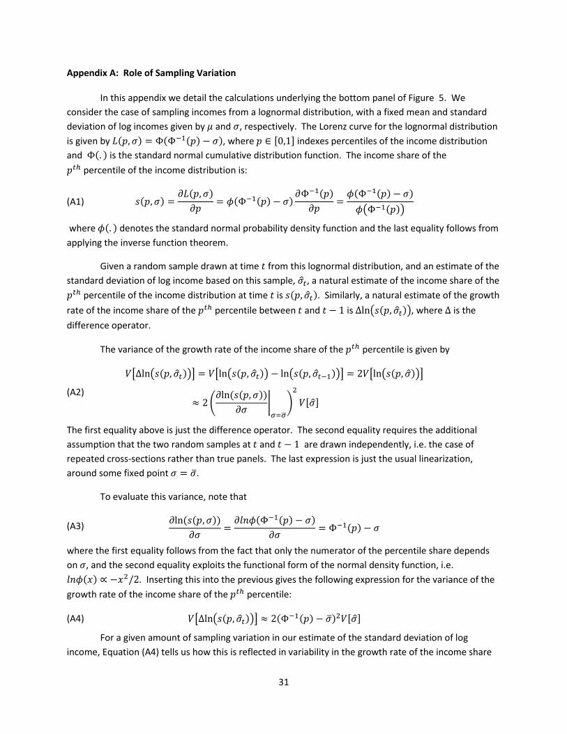
In Appendix A we derive an analytical expression for the standard deviation of the growth rates

of the income shares of different percentiles of the income distribution corresponding to this thought

experiment, which we plot in the bottom panel of Figure 5. This pattern is remarkably similar to what

we see in the actual data, with substantially higher volatility in the growth rate of the income shares of

the poorest deciles, despite the fact that there are no changes in relative incomes between the two

population distributions. This suggests that some of the apparent differences in the importance of

growth in average incomes for growth in social welfare that we saw in Table 2-Table 4 may simply

reflect the differential importance of sampling variation across decile shares.

17

We quantify this effect using the following illustrative calculation. The bottom panel of Figure 5

is based on the assumption that the household survey data comes from a simple random sample of

𝑛 = 5000 observations, and a standard deviation of log income of 𝜎 = 0.74, which corresponds to a

population Gini coefficient of 40, which is the average observed value in our data. The variance of the

growth rate of measured average income is the sum of the variance of true income growth, plus

sampling variation, which under our assumptions is simply 2𝜎2/𝑛.9 Based on this we can arrive at an

estimate of the true standard deviation of income growth, which is 4.0 percent, i.e. �0.0422 − 2 0.742

2500=

0.0396, as opposed to the observed standard deviation which is 4.2 percent.

Similarly, the observed standard deviation of the growth rates of the cumulative income shares

of the bottom 10, 20 and 40 percent will reflect both true variation as well as well as sampling variation.

Using the results in Appendix A, we can calculate the amount of sampling variation corresponding to our

assumption of 𝑛 = 50000 and 𝜎 = 0.74, and subtract this from the observed variance in income shares

to arrive at an estimate of their true standard deviations equal to 4.5 percent, 2.0 percent, and 1.6

percent for the income shares of the 10th, 20th and 40th percent (as opposed to the observed standard

deviations of 5.2 percent, 3.4 percent, and 2.3 percent, respectively). Finally, we use these estimates of

the true standard deviations of income growth and growth in income shares of the poorest to

recalculate the share of the variance of growth in social welfare due to growth in average incomes.10

This gives us larger variance shares, equal to 47 percent, 71 percent, and 86 percent for the income

shares of the 10th, 20th and 40th percent (as opposed to the 41 percent, 61 percent, and 78 percent as

reported in Table 2).

To sum up, we have seen that the share of the variance of growth in social welfare due to

growth in average incomes is smaller for more bottom-sensitive social welfare functions. This

mechanically reflects the fact that growth in income shares of lower deciles exhibits greater variability in

our dataset than those of higher deciles. However, we have seen that some of this greater variability in

income shares of the poorest may simply reflect measurement error due to sampling variation.

9 The growth rate of average income is the difference between the mean of log income in the first sample and the second sample. The variance of mean log income is 𝜎2/𝑛, and since the two samples are drawn indpendently, the variance of the difference in means is 2𝜎2/𝑛. 10 For this calculation, we assume that the true correlation between growth in the mean and changes in equality is the same as observed in the data. Since these observed correlations are small this assumption has little effect on our conclusions.

18

Adjusting for this suggests that the estimates of the share of the variance of growth in social welfare due

to growth in incomes reported in Table 2-Table 4 are likely to be lower bounds.

4.4 More General Social Welfare Functions and Generalized Lorenz Dominance

In all of our results thus far, we have relied on specific social welfare functions in order to be

able to explicitly measure the contribution of inequality changes to growth in social welfare. In

particular, the benefit of this approach is that it allows us to express inequality changes in terms of

growth in average incomes, which in turn leads to straightforward variance decompositions. Although

we have considered a variety of common social welfare functions, a drawback of this approach is that

our conclusions do depend on the specific functional form of the selected social welfare function. And

this in turn raises the possibility that there might be other social welfare functions for which the

contribution of growth to improvements in social welfare is much smaller (or larger) than for the ones

we have considered.

To partially address this concern, we draw on the concept of generalized Lorenz dominance to

determine the direction, although not the magnitude, of welfare changes for a much broader class of

social welfare functions than those considered here, over the same set of spells. Shorrocks (1983)

shows that as long as the social welfare function is increasing and concave in incomes (i.e. the social

welfare function prefers more income to less, and less inequality to more), then social welfare is

unambiguously higher if and only if the growth rate of cumulative average income of each percentile of

the population is positive. In our case where we focus on decile grouped data, this corresponds to the

case where growth in average incomes of the first decile, the first two deciles, etc. all the way up to

growth in overall average incomes, are all positive over a given spell. If this is true, then social welfare

will have improved over this spell for any social welfare function that satisfies the minimum

requirements of being increasing and concave in incomes.

To implement this, we divide our sample of spells into those with positive average growth rates

and those with negative average growth rates. In the first group, we count the number of spells where

the final distribution in each spell generalized-Lorenz-dominates the initial distribution. In the second

group, we do the opposite, counting up the number of spells where the initial distribution (before the

negative average growth experience) generalized-Lorenz-dominates the final distribution. In both cases,

these correspond to cases where positive (negative) growth unambiguously raised (lowered) social

welfare for any increasing and concave social welfare function.

19

The results of this calculation are shown in Table 6. Consider for example the 117 spells

comprising the long spells sample. 96 of these spells correspond to periods of positive average growth,

and of these, welfare unambiguously increases in fully 83 percent of spells. Conversely, for 57 percent

of the 21 spells with negative average growth, welfare unambiguously declined. Overall, welfare

changes in the same direction as average incomes in 78 percent of all spells. The small number of spells

in which mean income and social welfare have not unambiguously moved in the same direction are

generally ones in which the income growth rate is close to zero.

5. Policies, Growth, and Social Welfare

So far we have seen that most of the variation in growth rates in social welfare across countries

is due to cross-country differences in average growth. However, it may be important to understand the

factors underlying the remaining variation in social welfare growth due to changes in inequality. In

particular, if there were a combination of policies and institutions that resulted in the same growth rate

of average incomes as some other combination of policies, but also delivered a reduction in inequality,

then the inequality-reducing combination of policies would be preferable from the standpoint of

improving social welfare. In this section we use cross-country regression analysis to document more

systematically the relationship between a set of variables proxying for a variety of policy and

institutional factors on the one hand, and growth in social welfare and its components on the other.

Our starting point is the observation that each of the social welfare functions we consider is of

the form 𝑊 = 𝜇𝑔 where 𝜇 is mean income and 𝑔 is a decreasing function of some inequality measure.

For example, in the case of the Sen index, 𝑔 is one minus the Gini coefficient, which increases as

inequality falls. Similarly, in the case of the income of the bottom 40 percent, 𝑔 is equal to the income

share of the bottom 40 percent, which increases as inequality declines. For terminological convenience

we will refer to 𝑔 as “equality”. As discussed in the previous section, growth in social welfare is the sum

of growth in average income and growth in the relevant equality measure. We will consider a set of

empirical models for growth in social welfare, of the following form:

(9) ∆𝑙𝑛𝑊(𝑖, 𝑡) = 𝜌𝑗𝑙𝑛𝜇(𝑖, 𝑡 − 1) + 𝛾𝑗𝑙𝑛𝑔(𝑖, 𝑡 − 1) + 𝛽𝑗′𝑋𝑗(𝑖, 𝑡) + 𝜀𝑗(𝑖, 𝑡)

20

In every model, growth in social welfare depends on lagged log-levels of average income and inequality,

𝑙𝑛𝜇(𝑖, 𝑡 − 1) and 𝑙𝑛𝑔(𝑖, 𝑡 − 1), to pick up any convergence in social welfare. Each model is defined by

the specific set of right-hand-side variables 𝑋𝑗(𝑖, 𝑡) included in it, with 𝑗 indexing models. These

variables are taken from a set of proxies for various aspects of the policy and institutional environment

in the country. Naturally, the estimated coefficients on all right-hand-side variables, 𝜌𝑗, 𝛾𝑗, and 𝛽𝑗, vary

across models and therefore are also indexed by 𝑗.

This empirical specification allows us to decompose the contribution of various correlates of

social welfare growth into their effects on growth in average incomes and growth in equality. In

particular, Equation (9) above is the sum of a standard growth regression, as well as an analogous

specification for changes in equality:

(10) ∆𝑙𝑛𝜇(𝑖, 𝑡) = 𝜌𝜇𝑗𝑙𝑛𝜇(𝑖, 𝑡 − 1) + 𝛾𝜇𝑗𝑙𝑛𝑔(𝑖, 𝑡 − 1) + 𝛽𝜇𝑗′ 𝑋𝑗(𝑖, 𝑡) + 𝜀𝜇𝑗(𝑖, 𝑡)

(11) ∆𝑙𝑛𝑔(𝑖, 𝑡) = 𝜌𝑔𝑗𝑙𝑛𝜇(𝑖, 𝑡 − 1) + 𝛾𝑔𝑗𝑙𝑛𝑔(𝑖, 𝑡 − 1) + 𝛽𝑔𝑗′ 𝑋𝑗(𝑖, 𝑡) + 𝜀𝑔𝑗(𝑖, 𝑡)

where the estimated coefficients in the model for growth in social welfare are the sums of the

coefficients from the models for growth in average incomes and growth in equality, i.e. 𝜌𝑗 = 𝜌𝜇𝑗 + 𝜌𝑔𝑗;

𝛾𝑗 = 𝛾𝜇𝑗 + 𝛾𝑔𝑗; and 𝛽𝑗 = 𝛽𝜇𝑗 + 𝛽𝑔𝑗.

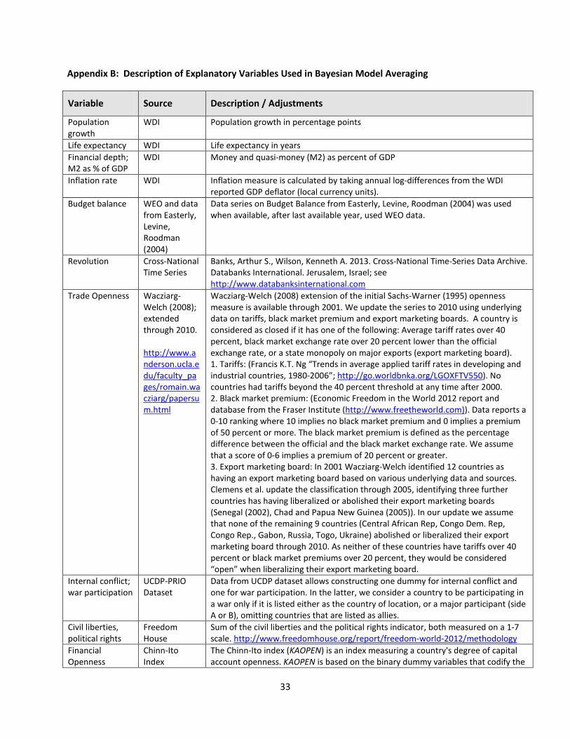
We consider as explanatory variables a set of variables that have been identified as important

correlates of growth in the large empirical cross-country growth literature. The growth correlates

include a measure of financial development (M2 as percentage of GDP), the Sachs-Warner indicator of

trade openness, the Chinn-Ito Index of financial openness, the inflation rate, the general government

budget balance, life expectancy, population growth, the Freedom House measure of civil liberties and

political rights, the frequency of revolutions, and a dummy variable indicating whether the country was

party to a civil or international war in a given year. Most of these variables have been identified as

important correlates of growth in one or more of three prominent meta-analyses of growth

determinants (Fernandez, Ley and Steel (2001a), Sala-i-Martin (2004) and Ciccone et al. (2010)). We

also consider some additional variables that have been found to be significant correlates of inequality in

the much smaller existing cross-country literature on determinants of inequality. These consist of

21

primary school enrollment rates, a measure of educational inequality11 (as emphasized by De Gregorio

et. al. (2002)), and the share of agriculture in GDP (as emphasized for example in Datt and Ravallion

(2002)).12 Appendix B provides a detailed description of the definitions and sources of all of these

variables.

In each model, 𝑋𝑗(𝑖, 𝑡) includes one particular combination of these 13 variables, and we will

consider all 213 = 8192 possible combinations of these variables. We rely on Bayesian Model

Averaging (BMA) as a tool to summarize the results from this large number of regression models. In

particular, BMA allows us to assign a posterior probability to each model, 𝑃[𝑀𝑗], which indicates the

relative likelihood of model 𝑗 compared with all of the other models considered. Intuitively, these

posterior probabilities reflect a tradeoff between goodness of fit and parsimony: for two models with

the same number of explanatory variables, the model that delivers the higher R-squared receives a

higher posterior probability. Similarly, for two models with the same R-squared, the model with fewer

explanatory variables receives a higher posterior probability.

We calculate the posterior model probabilities for the regression for overall social welfare

growth in Equation (9), and then use these to construct probability-weighted estimates of the slope

coefficients across all models, i.e.

(12) E�𝛽𝑗� = �𝑃[𝑀𝑗]2𝐾

𝑗=1

𝛽𝑗 = �𝑃[𝑀𝑗]2𝐾

𝑗=1

𝛽𝜇𝑗 + �𝑃[𝑀𝑗]2𝐾

𝑗=1

𝛽𝑔𝑗

This expression summarizes the estimated relationship between each of the explanatory variables and

growth in social welfare, averaging across all models. Moreover, it allows us to separate the effects

operating through growth and through increases in equality. Finally, for each variable we also calculate

a posterior inclusion probability (PIP). This is simply the sum of the posterior probabilities of each model

in which the variable appears, and is a useful summary of the relevance of that variable for growth in

11 Specifically, we use data on educational attainment by different levels of attainment from the Barro-Lee dataset to construct a (grouped) Lorenz curve summarizing the distribution of the total number of years of education across individuals, and from this calculate a corresponding Gini coefficient. 12 We also considered several other variables found to be significant correlates of inequality in some papers in the literature, but did not include them in our analysis because data coverage was very poor for many of the developing countries in our sample. These included indicators of labour market regulation and progressivity of tax systems (Checchi et. al. (2008)), public sector employment (Milanovic (2000) ), and social transfers (Milanovic (2000), De Gregorio et. al. (2002)).

22

social welfare. In particular, this measure identifies variables that appear in models that are more likely

relative to other models.

Table 7 summarizes our results. To conserve on space, we report results only for three social

welfare functions: average incomes in the bottom 40 percent, the Atkinson Index with 𝜃 = 3, and the

Sen Index. Our findings are qualitatively similar for the other social welfare functions considered in the

paper. Our dataset consists of the sample of spells of changes in social welfare over periods at least five

years long. Lagged log-levels of mean income and equality are measured at the beginning of each spell,

while the remaining 13 explanatory variables are measured as averages over the spells. Our sample

differs from the common practice in the cross-country empirical growth literature, which is to measure

growth over regularly-spaced five- or ten-year intervals. The advantage of our approach of working with

an irregularly-spaced panel is that it avoids the need to impute the household survey data across

different years within a country, but instead relates actual changes in equality to explanatory variables

observed over the same period. On the other hand, the disadvantage of this approach is that the

coefficients on initial income and initial equality in Equations (10) and (11) are more difficult to

interpret, because they reflect the rate of convergence over different time horizons. All of the

regressions are estimated by ordinary least squares (OLS).13

The first column in each panel reports the posterior inclusion probabilities for each variable.

The remaining three columns report the estimated coefficients for growth in social welfare, growth in

average incomes, and growth in equality, respectively. As discussed above, the slopes in the first

column are the sum of the slopes in the remaining two columns, i.e. the overall effect of a given variable

on growth in social welfare is the sum of its effects on growth in average incomes and on growth in

equality. To aid in the interpretation of the slopes, we scale each one to show to the effect on growth

(in percentage points per year) of a one standard deviation increase in the corresponding right-hand-

side variable. Below each estimated coefficient, we report in parentheses the percentage of all models

in which the estimated slope coefficient is statistically significant at the 95 percent level and is of the

13 Equations (10) and (11) are dynamic panel regressions, and the error terms are likely to include a country-specific time-invariance component (i.e. country effects). As such, they are subject to the usual concerns in the empirical growth literature about Nickell bias, as well as the usual concerns about potential endogeneity of other right-hand-side variables. Many papers in the empirical growth literature have sought to address these problems using the system-GMM estimator proposed by Arellano and Bond (1991). However, an under-appreciated concern with this approach is that the internal instruments based on appropriate lags and differences of explanatory variables are often weak in standard cross-country growth settings (see for example Bazzi and Clemens (2012)). We instead follow the recommendation of Hauk and Wacziarg (2010), who, following extensive Monte Carlo analysis of alternative estimators of growth regressions, conclude that pooled OLS performs best in practice.

23

same sign as the probability-weighted slope. Finally, note that the only difference across the three

panels in the growth regression is the choice of the initial inequality measure, which is different for each

social welfare function. As a result, the estimated coefficients on the remaining variables in the growth

regression are in most cases quite similar across the three panels.

Consider first the partial correlations between growth in social welfare and initial income and

initial equality. We assume these variables appear in all specifications, so by construction the posterior

inclusion probabilities are equal to one. The posterior probability-weighted estimated slopes in the

social welfare regression are negative in all cases, and are highly significant in the vast majority of

specifications, i.e. higher initial income levels, and higher initial equality, are significantly negatively

correlated with subsequent growth in social welfare. To understand this finding, it is useful to consider

separately the coefficients on these variables in the regressions for growth in average incomes, and

growth in equality. Consistent with the large empirical growth literature, we find that lower initial

income levels are associated with faster subsequent growth. The same is true of equality: lower initial

levels of equality, i.e. higher initial inequality, are significantly associated with faster subsequent growth

in equality, reflecting a tendency of equality to mean-revert.

On the other hand, we find little evidence that higher initial levels of equality are significantly

associated with subsequent growth, nor are initial income levels significantly associated with

subsequent changes in inequality. Specifically, initial equality is significantly positively correlated with

growth in only 4 percent of models (when the social welfare function is average incomes in the bottom

40 percent), and in 8 percent of models (when the social welfare function is the Sen index). This in turn

casts some doubt on the frequently-heard concern that higher initial inequality might undermine

subsequent growth. In fact, it is striking that even in the first and third panels, where the probability-

weighted slope coefficient on initial equality is positive in the growth regression (indicating a positive

partial correlation between greater equality and subsequent growth), the corresponding slope

coefficient is strongly negative in the social welfare regression. This is because any beneficial effects of

higher equality on subsequent growth in average incomes are offset by the tendency of equality to

mean-revert, which reduces social welfare through an increase in inequality.

Turning to the other variables in Table 7, some interesting patterns emerge. A few of them have

consistently high posterior inclusion probabilities, indicating that they are important partial correlates of

growth in social welfare in our sample. These include inflation (high inflation consistently is negatively

correlated with growth in social welfare); population growth (faster population growth is associated

24

with slower growth in social welfare); political instability as measured by revolutions (greater instability

leads to slower growth in social welfare); and the share of agriculture in GDP (a higher share is

associated with slower growth in social welfare). Interestingly, for each of these variables, the main

effect operates through the relationship with growth in average incomes: the coefficients in the third

column of each panel (which measure the partial correlations with growth) are much larger in absolute

value than the coefficients in the third column (which measure the partial correlations with changes in

equality). Consider for example the relationship between inflation and growth in social welfare. A one

standard deviation increase in inflation reduces average annual growth in social welfare by between 1.8

and 2.2 percent per year, depending on which social welfare function we consider. Nearly all of this

effect comes through lower growth in average incomes, which declines by 1.7 percentage points. This

estimated coefficient is significantly different from zero in all of the models in which it appears.14 The

probability-weighted slope coefficient from the equality regression is negative, suggesting that high

inflation is disequalizing on average. However, the estimated effect is much smaller than the estimated

effect on growth, and is rarely statistically significant.

Another interesting case is the relationship between growth in social welfare and the share of

agriculture in GDP, which is the one case among these four variables suggestive of a tradeoff. On the

one hand, a higher share of agriculture in GDP is associated with substantially slower growth in average

incomes, and this effect is significant in nearly all specifications. On the other hand, a higher share of

agriculture in GDP is positively associated with subsequent growth in equality. However, this latter

effect is once again much smaller than the effect on growth in average incomes, and moreover is never

statistically significant at conventional levels. As a result, the growth effect dominates, and the effect of

a larger share of agriculture in GDP on subsequent growth in social welfare is substantially negative.

It is however noteworthy that the remaining variables mostly have quite low posterior inclusion

probabilities, and rarely show up as significant correlates of either growth in average incomes or growth

in the relevant inequality measures. This is at least somewhat surprising, given that these variables

were selected for their prominence in the empirical growth literature. However, there are at least two

important differences between the empirical specifications here, and those in the majority of papers in

this broader literature. The first is that in our work, growth in average incomes is measured as growth in

average income or consumption from the underlying household survey. As we have noted earlier, there

are substantial differences between these growth rates and measures of mean growth taken from

14 This finding is in part driven by a fairly small number of spells with quite high inflation rates.

25

national accounts data. Second, the vast majority of papers in the empirical growth literature examine

growth over regularly-spaced spells of fixed length, typically five or ten years long, and with a much

larger set of observations. This contrasts with our sample, which is much smaller and irregularly-spaced,

as dictated by the limited availability of household survey data in particular years.

One way to assess the importance of these considerations is to re-estimate the results in Table

7, but replacing growth in household survey-based measures of average income with corresponding

data from the national accounts. In particular, we use real per capita GDP growth from the national

accounts, in order to be consistent with the empirical growth literature. However, we keep the

structure of our irregularly-spaced panel of observations determined by the availability of survey data.

For most variables, our findings are broadly similar to when we use household survey mean growth

rates. In addition, for some of our social welfare functions, we find that the budget balance has a

posterior inclusion probability greater than 0.5, and enters positively in the growth regressions,

suggesting that higher budget deficits are correlated with slower growth. One further notable finding is

that when we switch to national accounts growth rates, initial equality enters positively and significantly

in roughly three-quarters of all specifications for the growth regression, suggesting that initial inequality

is bad for subsequent growth. However, this does not imply that higher initial equality is good for

growth in social welfare. This is because, as we have already seen in Table 7, higher initial equality is

significantly correlated with subsequent declines in equality, and this effect is quantitatively larger than

the positive effect on average income growth. As a result, the posterior probability-weighted slope

coefficient on initial equality in the social welfare regression is still negative.

Conclusions

This paper is motivated by the widespread concerns about inequality and its consequences that

are often heard in current policy discussions. Our objective in this paper is to provide some simple

descriptive evidence on the implications of observed inequality for changes in social welfare. By

specifying a social welfare function, it is possible to quantify the welfare effects of changes in inequality,

and compare them with the welfare effects of growth in average incomes. In particular, we exploit the

fact that growth in a number of standard welfare functions can be decomposed into growth in average

incomes, and growth in a particular measure of inequality specific to each social welfare function.

We implement these decompositions in a large dataset of high-quality data on income and its

distribution across individuals, covering 117 countries over the past four decades. Using this data, we

26

construct a large set of non-overlapping episodes or spells of changes in average income and changes in

its distribution that are at least five years long, and measure the contribution of growth and changes in

inequality to growth in social welfare over each spell. Our basic findings are easily summarized. Most of

the cross-country and over-time variation in changes in social welfare is attributable to growth in

average incomes. In contrast, the contribution of changes in relative incomes to social welfare growth is

on average much smaller than growth in average incomes, and moreover is on average uncorrelated

with average income growth. These findings suggest that the welfare impacts of changes in inequality

observed over the past four decades are small when compared with the welfare impacts of growth in

average incomes.

We have also seen that the relative importance of inequality changes for social welfare growth

varies across the different types of social welfare functions we have considered. Specifically, the share

of the variance of growth in social welfare due to growth in average incomes is smaller the greater is the

weight that the social welfare function places on the poorest. For example, while the share of the

variance of growth in social welfare due to growth in average income is 77 percent when the social

welfare function is average incomes in the bottom 40 percent, it is 60 percent for the bottom 20

percent, and just 41 percent for the poorest 10 percent. Mechanically, this feature of our results is due

to the fact that the observed income shares of the poorest exhibit considerably more volatility than the

income share of those nearer to the middle of the income distribution. While some of this greater

volatility in income shares of the poorest surely is real, we also demonstrate that at least some of it may

simply be due to a differential effect of sampling variation on income shares at different points in the

income distribution. An illustrative correction for this suggests that the share of the variation in social

welfare growth due to growth in average incomes could be considerably higher even for social welfare

functions that attach positive weight only to the very poorest.

While the variation in the growth rate of most of the social welfare functions we consider that is

due to changes in inequality is on average substantially smaller than the share due to growth, it is

nevertheless potentially important to understand the factors underlying this variation. If, for example,

there were some combinations of policies that generated the same rate of average growth as another

combination, but at the same time reduced inequality, then the former combination might be

preferable from the standpoint of social welfare growth. To investigate this we consider a set of

variables intended to proxy for factors commonly thought to be conducive to growth in average

incomes. We use Bayesian Model Averaging as a tool to systematically document the partial

27

correlations between these variables and social welfare growth. We find that the relationship between

these variables and social welfare growth, to the extent that they are quantitatively important, comes

mostly through their effects on growth in average incomes, rather than through changes in inequality.

This of course does not imply that there are no policies that can influence inequality in ways that raise

social welfare. However, it does suggest that the historical experience of a large set of developed and

developing countries does not provide much guidance regarding the set of macroeconomic policies and

institutions that might be particularly conducive to promoting growth in social welfare beyond their

effects on aggregate growth.

References

Arellano, Manuel and Stephen Bond (1991). “Some Tests of Specification for Panel Data: Monte Carlo Evidence and an Application to Employment Questions”. Review of Economic Studies. 58(2)277-297. Atkinson, Anthony, Thomas Piketty, and Emmanual Saez (2011). “Top Incomes in the Long Run of History”. Journal of Economic Literature. 49(1):3-71. Bazzi, Samuel and Michael Clemens (2013). “Blunt Instruments: Avoiding Common Pitfalls in Identifying the Causes of Economic Growth”. American Economic Journal: Macroeconomics. 5(2):152-186. Basu, Susanto, Luigi Pascali, Fabio Schiantarelli, and Luis Serven (2013). “Productivity and the Welfare of Nations”. Manuscript, World Bank and Boston College. Checchi, Daniele; Garcia-Penalosa, Cecilia. (2008). “Labour Market Institutions and Income Inequality”, Economic Policy issue 56, pp. 601-34, 640-49. Chen, Shaohua, and Martin Ravallion. (2010). “The Developing World Is Poorer Than We Thought, But No Less Successful in the Fight against Poverty,” The Quarterly Journal of Economics. Ciccone, Antonia and Marek Jacocinski. (2010). “Determinants of Economics Growth: Will Data Tell?,” American Economic Journal: Macroeconomics 2, 2:4, 222-246. Datt, Gaurav, Ravallion, Martin (1992). “Growth and redistribution components of changes in poverty measures: a decomposition with applications to Brazil and India in the 1980s”. Journal of Development Economics 38(2):275–295. Deaton, Angus, and Valerie Kozel. (2005). “Data and Dogma: The Great Indian Poverty Debate”, Oxford University Press 20:177-199. De Gregorio, Jose; Lee, Jong-Wha. (2002). “Education and Income Inequality: New Evidence from Cross-Country Data”, Review of Income and Wealth, v. 48, iss. 3, pp. 395-416. Dollar, David, and Aart Kraay. (2002). “Growth is Good for the Poor,” Journal of Economic Growth, 7, 195-225.

28

Dollar, David, Tatjana Kleineberg, and Aart Kraay (2013). “Growth Still Is Good for the Poor”. World Bank Policy Research Department Working Paper No. 6568. Feldkircher, M., & Zeugner, S. (2009). Benchmark Priors Revisited: On Adaptive Shrinkage and the Supermodel Effect in Bayesian Model Averaging. IMF Working Paper No. 09/202, International Monetary Fund. Fernandez, C., Ley, E., & Steel, M.F.J. (2001a). Model Uncertainty in Cross-Country Growth Regressions. Journal of Applied Econometrics, 16(5), 563-576. Fernandez, C., Ley, E., & Steel, M.F.J. (2001b). Benchmark prior for Bayesian model averaging. Journal of Econometrics, 100(2), 381-427. Hauk, William and Romain Wacziarg (2009). “A Monte Carlo Study of Growth Regressions”. Journal of Economic Growth. 14:103-147. Jaumotte, Florence, Subir Lall, and Chris Papageorgiou. (2013). “Rising Income Inequality: Technology, or Trade and Financial Globalization,” IMF Economic Review, v. 61, no. 2, pp. 271-309. Jones, Chad and Peter Klenow (2011). "Beyond GDP: Welfare Across Countries and Time". Working Paper, Stanford University. Klenow, Peter and Andres Rodriguez-Clare (1997). “The Neoclassical Revival in Macroeconomics – Has It Gone Too Far?”, in Ben Bernanke and Julio Rotemberg, eds. NBER Macroeconomics Annual. Cambridge, MIT Press, pp. 72-103. Kraay, Aart (2006). “When Is Growth Pro-Poor? Evidence from a Panel of Countries”. Journal of Development Economics. 80:198-227. Lopez, J. Humberto and Luis Serven (2006). “A Normal Relationship? Growth, Inequality, and Poverty”. World Bank Policy Research Working Paper No. 3814. Milanovic, Branko. (2000). “Determinants of Cross-Country Income Inequality: An 'Augmented' Kuznets Hypothesis”, Essays in honour of Branko Horvat, pp. 48-79. Perri, Fabrizio and Dirk Krueger (2003). "On the Welfare Consequences of the Increase in Inequality in the US". NBER Macroeconomics Annual. Pew Research Center (2013). “Economies of Emerging Markets Better Rated During Difficult Times”. http://www.pewglobal.org/2013/05/23/economies-of-emerging-markets-better-rated-during-difficult-times/. Sala-i-Martin, Xavier, Gernot Doppelhofer, and Roland I. Miller. (2004). “Determinants of Long-Term Growth: A Bayesian Averaging of Classical Estimates (BACE) Approach.” American Economic Review, 94(4): 813-35. Sen, Amartya (1976). “Real National Income”. Review of Economic Studies.

29

Shorrocks, Anthony (1983). “Ranking Income Distributions”. Economica. February, pp. 3-17. World Bank (2013). “The World Bank Goals: End Extreme Poverty and Promote Shared Prosperity”. http://www.worldbank.org/content/dam/Worldbank/document/WB-goals2013.pdf.

30

Appendix A: Role of Sampling Variation In this appendix we detail the calculations underlying the bottom panel of Figure 5. We consider the case of sampling incomes from a lognormal distribution, with a fixed mean and standard deviation of log incomes given by 𝜇 and 𝜎, respectively. The Lorenz curve for the lognormal distribution is given by 𝐿(𝑝,𝜎) = Φ(Φ−1(𝑝) − 𝜎), where 𝑝 ∈ [0,1] indexes percentiles of the income distribution and Φ(. ) is the standard normal cumulative distribution function. The income share of the 𝑝𝑡ℎ percentile of the income distribution is:

(A1) 𝑠(𝑝,𝜎) =𝜕𝐿(𝑝,𝜎)𝜕𝑝

= 𝜙(Φ−1(𝑝)− 𝜎)𝜕Φ−1(𝑝)

𝜕𝑝=𝜙(Φ−1(𝑝) − 𝜎)𝜙�Φ−1(𝑝)�

where 𝜙(. ) denotes the standard normal probability density function and the last equality follows from applying the inverse function theorem.

Given a random sample drawn at time 𝑡 from this lognormal distribution, and an estimate of the standard deviation of log income based on this sample, 𝜎�𝑡, a natural estimate of the income share of the 𝑝𝑡ℎ percentile of the income distribution at time 𝑡 is 𝑠(𝑝,𝜎�𝑡). Similarly, a natural estimate of the growth rate of the income share of the 𝑝𝑡ℎ percentile between 𝑡 and 𝑡 − 1 is ∆ln�𝑠(𝑝,𝜎�𝑡)�, where ∆ is the difference operator.

The variance of the growth rate of the income share of the 𝑝𝑡ℎ percentile is given by

(A2)

𝑉�∆ln�𝑠(𝑝,𝜎�𝑡)�� = 𝑉�ln�𝑠(𝑝,𝜎�𝑡)� − ln�𝑠(𝑝,𝜎�𝑡−1)�� = 2𝑉�ln�𝑠(𝑝,𝜎�)��

≈ 2�𝜕ln (𝑠(𝑝,𝜎))

𝜕𝜎�𝜎=𝜎�

�2

𝑉[𝜎�]

The first equality above is just the difference operator. The second equality requires the additional assumption that the two random samples at 𝑡 and 𝑡 − 1 are drawn independently, i.e. the case of repeated cross-sections rather than true panels. The last expression is just the usual linearization, around some fixed point 𝜎 = 𝜎�.

To evaluate this variance, note that

(A3) 𝜕ln (𝑠(𝑝,𝜎))𝜕𝜎

=𝜕𝑙𝑛𝜙(Φ−1(𝑝) − 𝜎)

𝜕𝜎= Φ−1(𝑝) − 𝜎

where the first equality follows from the fact that only the numerator of the percentile share depends on 𝜎, and the second equality exploits the functional form of the normal density function, i.e. 𝑙𝑛𝜙(𝑥) ∝ −𝑥2/2. Inserting this into the previous gives the following expression for the variance of the growth rate of the income share of the 𝑝𝑡ℎ percentile:

(A4) 𝑉�∆ln�𝑠(𝑝,𝜎�𝑡)�� ≈ 2(Φ−1(𝑝)− 𝜎�)2𝑉[𝜎�]

For a given amount of sampling variation in our estimate of the standard deviation of log income, Equation (A4) tells us how this is reflected in variability in the growth rate of the income share

31

of the 𝑝𝑡ℎ percentile. The bottom panel of Figure 5 plots the theoretical standard deviation of the growth rate of the income share of the 𝑝𝑡ℎ percentile, linearizing around the point 𝜎� = 0.74, corresponding to a Gini coefficient 0.4, which is roughly the mean of all the Gini coefficients in our

sample. The level of this series is arbitrary and depends on what we assume for �𝑉[𝜎�] = 𝜎/√2𝑛. We assume that = 0.74 , and to roughly match the data in the top panel of Figure 5 we assume a sample size of 𝑛 = 5000. While many of the household surveys in our dataset have much larger samples, it is worth keeping in mind that they rarely are simple random samples as is assumed here, and so the effective sample size is much smaller.

To make the adjustments to the growth rates of the cumulative decile shares implied by this calculation, note first that, following the same steps as above, the variance of the growth rate of the 𝑝𝑡ℎ cumulative decile share is:

(A5) 𝑉�∆ln�𝐿(𝑝,𝜎�𝑡)�� = 2𝑉�ln�𝐿(𝑝,𝜎�)�� ≈ 2�𝜙(Φ−1(𝑝)− 𝜎)Φ(Φ−1(𝑝) − 𝜎)�

2

𝑉[𝜎�]

32

Appendix B: Description of Explanatory Variables Used in Bayesian Model Averaging

Variable

Source

Description / Adjustments

Population growth

WDI Population growth in percentage points

Life expectancy WDI Life expectancy in years Financial depth; M2 as % of GDP

WDI Money and quasi-money (M2) as percent of GDP

Inflation rate WDI Inflation measure is calculated by taking annual log-differences from the WDI reported GDP deflator (local currency units).

Budget balance WEO and data from Easterly, Levine, Roodman (2004)

Data series on Budget Balance from Easterly, Levine, Roodman (2004) was used when available, after last available year, used WEO data.

Revolution Cross-National Time Series

Banks, Arthur S., Wilson, Kenneth A. 2013. Cross-National Time-Series Data Archive. Databanks International. Jerusalem, Israel; see http://www.databanksinternational.com

Trade Openness

Wacziarg-Welch (2008); extended through 2010. http://www.anderson.ucla.edu/faculty_pages/romain.wacziarg/papersum.html

Wacziarg-Welch (2008) extension of the initial Sachs-Warner (1995) openness measure is available through 2001. We update the series to 2010 using underlying data on tariffs, black market premium and export marketing boards. A country is considered as closed if it has one of the following: Average tariff rates over 40 percent, black market exchange rate over 20 percent lower than the official exchange rate, or a state monopoly on major exports (export marketing board). 1. Tariffs: (Francis K.T. Ng “Trends in average applied tariff rates in developing and industrial countries, 1980-2006”; http://go.worldbnka.org/LGOXFTV550). No countries had tariffs beyond the 40 percent threshold at any time after 2000. 2. Black market premium: (Economic Freedom in the World 2012 report and database from the Fraser Institute (http://www.freetheworld.com)). Data reports a 0-10 ranking where 10 implies no black market premium and 0 implies a premium of 50 percent or more. The black market premium is defined as the percentage difference between the official and the black market exchange rate. We assume that a score of 0-6 implies a premium of 20 percent or greater. 3. Export marketing board: In 2001 Wacziarg-Welch identified 12 countries as having an export marketing board based on various underlying data and sources. Clemens et al. update the classification through 2005, identifying three further countries has having liberalized or abolished their export marketing boards (Senegal (2002), Chad and Papua New Guinea (2005)). In our update we assume that none of the remaining 9 countries (Central African Rep, Congo Dem. Rep, Congo Rep., Gabon, Russia, Togo, Ukraine) abolished or liberalized their export marketing board through 2010. As neither of these countries have tariffs over 40 percent or black market premiums over 20 percent, they would be considered “open” when liberalizing their export marketing board.

Internal conflict; war participation

UCDP-PRIO Dataset

Data from UCDP dataset allows constructing one dummy for internal conflict and one for war participation. In the latter, we consider a country to be participating in a war only if it is listed either as the country of location, or a major participant (side A or B), omitting countries that are listed as allies.

Civil liberties, political rights

Freedom House

Sum of the civil liberties and the political rights indicator, both measured on a 1-7 scale. http://www.freedomhouse.org/report/freedom-world-2012/methodology

Financial Openness

Chinn-Ito Index

The Chinn-Ito index (KAOPEN) is an index measuring a country's degree of capital account openness. KAOPEN is based on the binary dummy variables that codify the

33

tabulation of restrictions on cross-border financial transactions reported in the IMF's Annual Report on Exchange Arrangements and Exchange Restrictions (AREAER). http://web.pdx.edu/~ito/Chinn-Ito_website.htm

Primary schooling

WDI Gross primary school enrollment rates (percent of population)

Gini coefficient on educational attainment

Barro-Lee dataset

The Barro-Lee dataset provides data on the percentage of the population that attained different levels of education: No education (0 years), complete primary (6 years), complete secondary (12 years), and complete tertiary (16 years). For non-complete primary, secondary, or tertiary we assume respectively 3 years, 9 years, and 14 years of schooling. With this information, we can construct a Lorenz curve measuring which percentage of population attained which percentage of total years of schooling. With this information, we construct a Gini coefficient that measures educational inequality analogous to the standard income inequality measure.

Agricultural Share in GDPproductivity

WDI WDI Indicator: NV.AGR.TOTL.ZS, “Agriculture, value added (% of GDP)”.

34

Figure 1: Weights On Incomes and Individuals Implied by Social Welfare Functions

Panel A: Weights on Incomes

Panel B: Weights on Individuals

Notes: The top panel shows the weights (on the vertical axis) assigned by the indicated social welfare functions to the incomes of individuals at different points in the income distribution (on the horizontal axis). The bottom panel reports the same information, but for the weights assigned to individuals rather than incomes. Weights are normalized to sum to one. Weights are in general data-dependent and are depicted for a hypothetical lognormal income distribution with a mean of $2000 per annum and a Gini coefficient equal to 30.

0

0.001

0.002

0.003

0.004

0.005

0 0.2 0.4 0.6 0.8 1

Wei

ght o

n In

com

e of

Per

cent

ile j

in

Soci

al W

elfa

re F

unct

ion

Percentile of Income Distribution

Bottom40

Sen

Atkinson(0)

Atkinson(1)

Atkinson (2)

0

0.0005

0.001

0.0015

0.002

0.0025

0.003

0.0035

0.004

0.0045

0.005

0 0.2 0.4 0.6 0.8 1

Wei

ght o

n Pe

rcen

tile

j in

Soci

al W

elfa

re

Func

tion

Percentiles of Income Distribution

Bottom40

Sen

Atkinson(0)

Atkinson(1)

Atkinson (2)

35

Figure 2: Availability of Household Survey Data (POVCALNET and LIS)

Notes: This figure shows number of household surveys available in each year, for the LIS and POVCALNET databases.

0

10

20

30

40

50

60

1967

1969

1971

1973

1975

1977

1979

1981

1983

1985

1987

1989

1991

1993

1995

1997

1999

2001

2003

2005

2007

2009

2011

LIS Database (# obs) PCN Database (#obs)

36

Figure 3: Growth in Average Incomes and Growth in Social Welfare

Bottom 10%

Bottom 20%

Bottom 40%

Bottom 90%

Figure continues on following page

37

Figure , Cont’d: Growth in Average Incomes and Growth in Social Welfare

Atkinson Index A(1)

Atkinson Index A(2)

Atkinson Index A(3)

Sen Index

Notes: This graph plots the average annual growth rate in average income (on the horizontal axis) against average annual growth rate in social welfare (on the vertical axis), for each indicated social welfare function. All growth rates are constant price annual average log-differences. The dataset consists of the sample of 285 non-overlapping spells lasting at least five years.

38

Figure 4: Distribution of Growth in Average Incomes and Growth in Inequality

Bottom 10, 20, 40 and 90 Percent

Atkinson A(1) A(2) A(3) and Sen Indices

Notes: This graph shows the kernel density estimate of the distribution of the growth rate of average income, and the growth rate of the inequality change component of the indicated social welfare functions. The dataset consists of the sample of 284 non-overlapping spells lasting at least five years.

39

Figure 5: Standard Deviation of Growth Rate of Income Shares

Actual (Decile Shares, Sample of Min-5 Year Spells)

Artificial (Sampling Variation Only, No Changes in True Decile Shares)

Notes: The top panel reports the standard deviation (across spells) of the average annual growth rate of the indicated decile share, in the sample of spells at least five years long. The bottom panel graphs the hypothetical standard deviation of the growth rate of the income share of each percentile of the income distribution under the assumption that the only source of variation across spells is sampling variation, i.e. the population mean and variance of log income are the same at both endpoints of each spell.

0

0.01

0.02

0.03

0.04

0.05

0.06

D1 D2 D3 D4 D5 D6 D7 D8 D9 D10

Stan

dard

Dev

iatio

n of

Gro

wth

Rat

e of

De

cile

Sha

re

0

0.01

0.02

0.03

0.04

0.05

0.06

0 0.2 0.4 0.6 0.8 1

Stan

dard

Dev

iatio

n of

Gro

wth

Rat

e of

Pe

rcen

tile

Shar

e

Percentile p

40

Table 1: Descriptive Statistics

Notes: This table reports the mean, standard deviation, and 10th and 90th percentiles of the distribution of growth rates of average income (the first column) and the relevant inequality measure corresponding to the indicated social welfare function (the remaining eight columns). The top panel pools all countries and periods. The middle panel distinguishes countries by their income level. The bottom panel reports results by decades. In the bottom panel, each subsample consists of all spells with at least one end-point in the indicated decade. Spells are weighted by the fraction of years of the spell falling in the indicated decade. The dataset in the second and third panels consists of the sample of 284 non-overlapping spells at least five years long.

Social Welfare Function Average incomes

Bottom 10%

Bottom 20%

Bottom 40%

Bottom 90%

Atkinson Index (1)

Atkinson Index (2)

Atkinson Index (3) Sen Index

Sample 1: Long Spells (N=117)Mean 0.020 0.006 0.005 0.003 0.001 0.002 0.003 0.004 0.001

Std. Dev. 0.028 0.033 0.025 0.018 0.008 0.009 0.018 0.024 0.010P10 -0.011 -0.022 -0.018 -0.015 -0.008 -0.006 -0.012 -0.016 -0.010P90 0.052 0.042 0.034 0.025 0.012 0.013 0.025 0.031 0.014

Sample 2: Min-5-year Spells (N=285)Mean 0.015 0.002 0.001 0.000 0.000 0.000 0.001 0.002 0.000

Std. Dev. 0.042 0.052 0.034 0.023 0.010 0.012 0.028 0.040 0.012P10 -0.028 -0.053 -0.039 -0.027 -0.012 -0.014 -0.028 -0.038 -0.015P90 0.063 0.061 0.045 0.031 0.012 0.016 0.031 0.041 0.016

Low Income (N=42)Mean 0.025 0.010 0.007 0.004 0.001 0.002 0.005 0.007 0.002

Std. Dev. 0.035 0.051 0.040 0.029 0.015 0.016 0.029 0.038 0.017P10 -0.012 -0.037 -0.027 -0.028 -0.016 -0.015 -0.022 -0.025 -0.018P90 0.058 0.076 0.061 0.039 0.023 0.021 0.036 0.055 0.025

Middle Income (N=168)Mean 0.013 0.003 0.002 0.001 0.000 0.001 0.002 0.003 0.000

Std. Dev. 0.049 0.057 0.036 0.024 0.010 0.013 0.032 0.046 0.013P10 -0.037 -0.060 -0.047 -0.034 -0.013 -0.016 -0.030 -0.042 -0.017P90 0.079 0.064 0.047 0.034 0.014 0.017 0.033 0.048 0.018

High Income (N=75)Mean 0.016 -0.004 -0.004 -0.004 -0.002 -0.001 -0.002 -0.003 -0.002

Std. Dev. 0.026 0.037 0.021 0.014 0.006 0.006 0.014 0.022 0.008P10 -0.013 -0.041 -0.031 -0.022 -0.009 -0.009 -0.016 -0.025 -0.012P90 0.051 0.036 0.022 0.012 0.004 0.006 0.015 0.023 0.006

1980s (N = 80)Mean 0.002 -0.002 -0.001 -0.002 -0.001 -0.001 -0.001 -0.002 -0.001

Std. Dev. 0.045 0.037 0.026 0.019 0.010 0.009 0.018 0.025 0.011P10 -0.058 -0.045 -0.035 -0.022 -0.013 -0.011 -0.018 -0.034 -0.015P90 0.048 0.034 0.024 0.017 0.009 0.008 0.015 0.022 0.010

1990s (N = 198)Mean 0.008 -0.006 -0.004 -0.003 -0.001 -0.001 -0.003 -0.004 -0.002

Std. Dev. 0.044 0.054 0.035 0.024 0.011 0.013 0.029 0.041 0.013P10 -0.037 -0.073 -0.051 -0.034 -0.014 -0.016 -0.031 -0.045 -0.018P90 0.055 0.060 0.043 0.033 0.015 0.017 0.031 0.038 0.018

2000s (N=167)Mean 0.029 0.012 0.007 0.004 0.001 0.002 0.006 0.010 0.001

Std. Dev. 0.036 0.052 0.034 0.023 0.010 0.012 0.029 0.042 0.012P10 -0.014 -0.030 -0.024 -0.021 -0.010 -0.010 -0.018 -0.023 -0.013P90 0.080 0.075 0.053 0.034 0.012 0.018 0.039 0.057 0.017

All Observations (Pooled)

By Decade (Min-5-year Spells)

By Income Category (Min-5-year Spells)

41

Table 2: Regressions of Social Welfare Growth on Average Income Growth

Notes: This table reports the results from a regression of growth in the indicated social welfare function (in each column) on growth in average incomes, in the sample of non-overlapping spells lasting at least five years (Panel A), and in the sample of long spells with one spell per country (Panel B). Heteroskedasticity-consistent standard errors reported in parentheses. * (**) (***) indicate significant differences from zero at the 10 (5) (1) percent level. The last row in each panel reports the p-value associated with the test of the null hypothesis that the estimated slope coefficient is equal to one.

(1) (2) (3) (4) (5) (6) (7) (8)

Social Welfare Function Bottom 10% Bottom 20% Bottom 40% Bottom 90% Atkinson Index (1)

Atkinson Index (2)

Atkinson Index (3) Sen Index

Avg. growth - Min 5 year spells 1.151*** 1.075*** 1.021*** 0.991*** 1.008*** 1.043*** 1.083*** 1.003***(0.0842) (0.0626) (0.0467) (0.0223) (0.0238) (0.0468) (0.0640) (0.0273)

Number of Observations 285 285 285 285 285 285 285 285R-squared 0.476 0.650 0.783 0.944 0.925 0.717 0.571 0.921Variance decomposition 0.413 0.605 0.767 0.952 0.918 0.687 0.527 0.918P-val. wald test, slope=1 0.0765 0.234 0.654 0.687 0.749 0.362 0.197 0.903

Avg. growth - Long spells 0.961*** 0.953*** 0.955*** 0.975*** 0.970*** 0.943*** 0.932*** 0.974***(0.162) (0.119) (0.0785) (0.0249) (0.0382) (0.0835) (0.118) (0.0376)

Number of Observations 117 117 117 117 117 117 117 117R-squared 0.403 0.535 0.685 0.927 0.897 0.688 0.538 0.887Share of variance due to growth 0.420 0.561 0.718 0.951 0.924 0.730 0.578 0.911P-val. wald test, slope=1 0.810 0.696 0.569 0.324 0.435 0.496 0.565 0.497

Panel A: Sample with spells of minimum 5 year length

Panel B: Sample with longest spell per country

42

Table 3: Regressions of Social Welfare Growth on Average Income Growth: Min 5-Year Spells Disaggregated By Income Level

Notes: This table reports the results from a regression of growth in the indicated social welfare function (in each column) on growth in average incomes, in the sample of non-overlapping spells lasting at least five years. The three panels correspond to sets of countries at different income levels, following the World Bank’s classification for 2012. Heteroskedasticity-consistent standard errors reported in parentheses. * (**) (***) indicate significant differences from zero at the 10 (5) (1) percent level. The last row in each panel reports the p-value associated with the test of the null hypothesis that the estimated slope coefficient is equal to one.

(1) (2) (3) (4) (5) (6) (7) (8)

Social Welfare Function Bottom 10% Bottom 20% Bottom 40% Bottom 90% Atkinson Index (1)

Atkinson Index (2)

Atkinson Index (3) Sen Index

Avg. growth 1.253*** 1.030*** 0.950*** 0.947*** 0.977*** 1.021*** 1.102*** 0.953***(0.255) (0.156) (0.106) (0.0469) (0.0504) (0.105) (0.163) (0.0635)

Number of Observations 75 75 75 75 75 75 75 75R-squared 0.441 0.600 0.755 0.947 0.939 0.776 0.615 0.904Variance decomposition 0.352 0.583 0.795 1.000 0.961 0.761 0.558 0.948P-val. wald test, slope=1 0.329 0.850 0.644 0.268 0.659 0.846 0.536 0.468

Avg. growth 1.164*** 1.091*** 1.033*** 0.997*** 1.013*** 1.055*** 1.097*** 1.011***(0.0955) (0.0719) (0.0544) (0.0264) (0.0279) (0.0544) (0.0737) (0.0319)

Number of Observations 168 168 168 168 168 168 168 168R-squared 0.509 0.693 0.819 0.958 0.936 0.728 0.583 0.939Share of variance due to growth 0.438 0.636 0.793 0.960 0.924 0.690 0.531 0.929P-val. wald test, slope=1 0.0911 0.211 0.551 0.922 0.630 0.317 0.193 0.728

Avg. growth 0.899*** 0.951*** 0.967*** 0.975*** 0.978*** 0.947*** 0.923*** 0.975***(0.291) (0.216) (0.145) (0.0535) (0.0742) (0.159) (0.223) (0.0722)

Number of Observations 42 42 42 42 42 42 42 42R-squared 0.269 0.409 0.569 0.836 0.820 0.569 0.418 0.801Share of variance due to growth 0.299 0.430 0.588 0.858 0.839 0.600 0.453 0.821P-val. wald test, slope=1 0.732 0.823 0.821 0.650 0.769 0.744 0.732 0.733

Panel A: High Income Countries

Panel B: Middle Income Countries

Panel C: Low Income Countries

43

Table 4: Regressions of Social Welfare Growth on Average Income Growth: Min 5-Year Spells Disaggregated By Decade

Notes: This table reports the results from a regression of growth in the indicated social welfare function (in each column) on growth in average incomes, in the sample of non-overlapping spells lasting at least five years. The three panels correspond to the indicated time periods. The regression for each decade includes all spells with at least one end-point falling in the indicated decade. Spells are weighted by the fraction of the years of the spell falling in the indicated decade. Heteroskedasticity-consistent standard errors reported in parentheses. * (**) (***) indicate significant differences from zero at the 10 (5) (1) percent level. The last row in each panel reports the p-value associated with the test of the null hypothesis that the estimated slope coefficient is equal to one.

(1) (2) (3) (4) (5) (6) (7) (8)

Social Welfare Function Bottom 10% Bottom 20% Bottom 40% Bottom 90% Atkinson Index (1) Atkinson Index (2) Atkinson Index (3) Sen Index

Avg. growth 1.120*** 1.061*** 1.016*** 0.980*** 0.995*** 1.019*** 1.049*** 0.998***(0.133) (0.0991) (0.0753) (0.0388) (0.0375) (0.0689) (0.0941) (0.0468)

Number of Observations 80 80 80 80 80 80 80 80R-squared 0.664 0.782 0.859 0.956 0.959 0.870 0.780 0.943Variance decomposition 0.593 0.737 0.846 0.975 0.964 0.854 0.743 0.945P-val. wald test, slope=1 0.369 0.542 0.835 0.616 0.904 0.785 0.604 0.961

Avg. growth 1.127*** 1.062*** 1.013*** 0.983*** 0.999*** 1.025*** 1.058*** 0.998***(0.0979) (0.0757) (0.0590) (0.0297) (0.0306) (0.0559) (0.0739) (0.0349)

Number of Observations 198 198 198 198 198 198 198 198R-squared 0.468 0.650 0.779 0.940 0.924 0.716 0.569 0.919Share of variance due to growth 0.415 0.612 0.769 0.956 0.924 0.699 0.538 0.921P-val. wald test, slope=1 0.196 0.417 0.824 0.579 0.977 0.662 0.436 0.950

Avg. growth 1.018*** 0.996*** 0.970*** 0.985*** 0.990*** 0.991*** 1.000*** 0.982***(0.119) (0.0776) (0.0505) (0.0189) (0.0261) (0.0638) (0.0935) (0.0260)

Number of Observations 167 167 167 167 167 167 167 167R-squared 0.326 0.517 0.699 0.931 0.890 0.589 0.416 0.895Share of variance due to growth 0.320 0.519 0.720 0.945 0.899 0.595 0.416 0.911P-val. wald test, slope=1 0.879 0.959 0.557 0.444 0.709 0.887 0.996 0.481

Panel C: 2000s

Panel A: 1980s

Panel B: 1990s

44

Table 5: Regressions of Social Welfare Growth on Average Income Growth:

Alternative Measures of Real Income Growth

Notes: This table reports the results from a regression of growth in the indicated social welfare function (in each column) on growth in average incomes, in the sample of non-overlapping spells lasting at least five years. The three panels correspond to the three different measures of mean income. Heteroskedasticity-consistent standard errors reported in parentheses. * (**) (***) indicate significant differences from zero at the 10 (5) (1) percent level. The last row in each panel reports the p-value associated with the test of the null hypothesis that the estimated slope coefficient is equal to one.

(1) (2) (3) (4) (5) (6) (7) (8)

Bottom 10% Bottom 20% Bottom 40% Bottom 90% Atkinson Index (1)

Atkinson Index (2)

Atkinson Index (3) Sen Index

Avg. growth - Min 5 year spells 1.075*** 1.006*** 0.965*** 0.963*** 0.983*** 1.005*** 1.038*** 0.967***(0.100) (0.0695) (0.0501) (0.0238) (0.0275) (0.0572) (0.0798) (0.0283)

Number of Observations 274 274 274 274 274 274 274 274R-squared 0.383 0.565 0.722 0.927 0.902 0.645 0.485 0.899Share of variance due to growth 0.356 0.561 0.749 0.963 0.917 0.642 0.467 0.929P-value of wald test, slope=1 0.454 0.930 0.481 0.123 0.545 0.934 0.638 0.254

Avg. growth - Min 5 year spells 1.146*** 1.051*** 1.011*** 0.997*** 1.011*** 1.060*** 1.105*** 1.002***(0.0938) (0.0648) (0.0463) (0.0212) (0.0241) (0.0513) (0.0723) (0.0259)

Number of Observations 274 274 274 274 274 274 274 274R-squared 0.301 0.463 0.634 0.891 0.855 0.552 0.394 0.851Share of variance due to growth 0.262 0.440 0.626 0.894 0.846 0.521 0.357 0.849P-value of wald test, slope=1 0.122 0.433 0.805 0.882 0.660 0.241 0.148 0.925

Avg. growth - Min 5 year spells 1.133*** 1.030*** 0.977*** 0.969*** 0.992*** 1.034*** 1.082*** 0.975***(0.109) (0.0768) (0.0551) (0.0262) (0.0299) (0.0607) (0.0846) (0.0312)

Number of Observations 274 274 274 274 274 274 274 274R-squared 0.299 0.457 0.621 0.888 0.852 0.543 0.388 0.847Share of variance due to growth 0.264 0.443 0.636 0.916 0.859 0.526 0.358 0.869P-value of wald test, slope=1 0.226 0.696 0.677 0.232 0.782 0.581 0.334 0.423

Panel C: Mixed measure (arithmetic average from A&B)

Different Welfare Measures

Panel A: Survey data (income or consumption)

Panel B: Real private consumption per capita (National accounts data)

45

Table 6: Welfare Comparisons Using Generalized Lorenz Dominance

Notes: This table summarizes the results of a generalized Lorenz dominance comparison of the initial and final income distributions of each spell in the indicated sample. The first two columns consider spells with positive growth in the survey mean and report the fraction of cases for which the end-point distribution of the spell generalized Lorenz-dominates the initial distribution. The second two columns do the reverse for spells with negative growth in average incomes. The last two columns combine information for all spells.

Number of spellsProportion for which welfare unambiguously increased Number of spells

Proportion for which welfare unambiguously decreased Number of spells

Proportion for which welfare unambiguously changed

Min 5 year spells 203 81% 82 65% 284 76%

Longest Spell per country 97 85% 20 57% 117 79%

Positive Growth Spells Negative Growth Spells All Spells

46

Table 7: Policies and Social Welfare Growth

Notes: This table summarizes selected BMA results. The three panels correspond to specifications using the three indicated social welfare functions. Within each panel, the first column reports the posterior inclusion probability for the indicated explanatory variable. The second column within each panel reports the posterior probability-weighted estimated slope coefficients for the growth rate of social welfare (Equation (9)). The third and fourth columns within each panel report the corresponding posterior probability-weighted slopes for the regressions where growth in average incomes, and growth in the relevant equality measure, are the dependent variable. As discussed in the text, these two slope coefficients sum to the slope coefficient reported in the second column, and they are multiplied by the standard deviation of the corresponding right-hand-side variable. The number in parentheses indicate the fraction of models in which the estimated slope coefficient is statistically significantly different from zero and of the same sign as the posterior probability-weighted slope.

Posterior Inclusion

ProbabilitySocial

Welfare Growth Equality

Posterior Inclusion

ProbabilitySocial

Welfare Growth Equality

Posterior Inclusion

ProbabilitySocial

Welfare Growth Equality

Initial income level 1.000 -2.835 -3.055 0.219 1.000 -2.832 -3.015 0.184 1.000 -2.900 -3.081 0.181(100) (100) (0) (98) (100) (0) (100) (100) (1)

Initial equality level 1.000 -1.011 0.078 -1.089 1.000 -2.042 -0.005 -2.037 1.000 -0.496 0.118 -0.615(94) (4) (100) (100) (0) (100) (14) (8) (100)

Financial depth (M2 % GDP) 0.003 -0.001 -0.002 0.001 0.004 0.000 -0.002 0.002 0.002 -0.001 -0.001 0.000(0) (2) (11) (0) (2) (18) (0) (2) (20)

Inflation rate 1.000 -1.980 -1.692 -0.288 1.000 -2.242 -1.705 -0.537 1.000 -1.841 -1.694 -0.147(100) (100) (12) (99) (100) (20) (100) (100) (7)

Budget Balance 0.000 0.000 0.000 0.000 0.000 0.000 0.000 0.000 0.000 0.000 0.000 0.000(23) (44) (0) (19) (41) (0) (31) (47) (0)

Trade Openness 0.004 0.001 0.002 -0.001 0.004 0.001 0.002 -0.001 0.008 0.003 0.003 -0.001(21) (26) (0) (13) (26) (0) (25) (26) (0)

Population growth 0.575 -0.508 -0.394 -0.114 0.762 -0.904 -0.519 -0.385 0.563 -0.452 -0.380 -0.071(51) (10) (48) (95) (14) (88) (24) (8) (66)

Life expectancy 0.039 0.006 0.016 -0.010 0.037 0.000 0.015 -0.014 0.048 0.015 0.020 -0.005(1) (11) (2) (1) (12) (1) (6) (11) (1)

Revolutions per pop. 0.470 -0.288 -0.276 -0.012 0.308 -0.226 -0.191 -0.036 0.579 -0.351 -0.331 -0.020(44) (54) (0) (39) (57) (0) (54) (53) (0)

Civil Liberties / Democracy 0.031 -0.008 -0.010 0.003 0.027 -0.001 -0.008 0.008 0.035 -0.010 -0.012 0.002(0) (0) (0) (0) (0) (0) (0) (0) (0)

Internal/external conflict (dummy 0.034 0.002 -0.002 0.005 0.038 0.007 -0.001 0.009 0.033 0.000 -0.002 0.003(1) (0) (0) (1) (0) (0) (0) (0) (0)

Fin. openness (Chinn-Ito) 0.000 0.000 0.000 0.000 0.000 0.000 0.000 0.000 0.000 0.000 0.000 0.000(13) (9) (0) (24) (10) (0) (12) (9) (0)

Primary school enrollment rate 0.003 0.000 0.001 -0.001 0.004 -0.002 0.001 -0.003 0.008 0.002 0.003 -0.001(3) (2) (68) (33) (1) (97) (0) (2) (50)

Education Gini 0.001 0.000 0.000 0.000 0.000 0.000 0.000 0.000 0.001 0.000 0.000 0.000(17) (34) (0) (14) (35) (0) (25) (31) (0)

Agriculture (% GDP) 0.997 -1.969 -2.265 0.296 0.969 -1.701 -2.197 0.496 0.999 -2.090 -2.260 0.171(88) (100) (0) (51) (100) (0) (100) (100) (0)

Panel C: SWF is Sen IndexPanel A: SWF is Bottom 40 Percent Panel B: SWF is Atkinson Index (Theta=3)

47