GROWTH OF BOUNDARY LAYER ON SMOOTH AND ROUGH … · 2017-04-18 · In Fluid flow, the Reynolds...

GROWTH OF BOUNDARY LAYER ON SMOOTH AND

ROUGH SURFACE

A THESIS SUBMITTED IN

PARTIAL FULFILLMENT OF THE REQUIREMENT

FOR THE DEGREE OF

Bachelor of Technology

In

Civil Engineering Department

By

Ravi Kumar Sahu (111ce0051)

Under the Guidance of

Dr. AWADHESH KUMAR

DEPARTMENT OF CIVIL ENGINEERING

NATIONAL INSTITUTE OF TECHNOLOGY, ROURKELA

May, 2015

CERTIFICATE

This is to certify that the thesis report entitled “growth of boundary layer on smooth and

rough surfaces”in partial fulfilment of the requirements for the award of BACHELOR OF

TECHNOLOGY Degree in Civil Engineering Department at the National Institute of

Technology, Rourkela (Deemed University) is an authentic work carried out by him under my

supervision and guidance.

To the best of my knowledge, the matter embodied in the thesis has not been submitted to any

other University/ Institute for the award of any degree or diploma.

Date: Prof. A. Kumar

Department of Civil Engineering,

National Institute of Technology Rourkela,

769008

ACKNOWLEDGEMENT

We would like to express our sincere gratitude to Dr.A.Kumar for his invaluable guidance,

cooperation and constant encouragement during the course of the project. We are grateful to

Dr.S.K Sahu ,Head of the Department, Civil Engineering for giving a lot of freedom ,

encouragement and guidance .We are also thankful to the Technical staff of the Fluid

Mechanics Laboratory, NIT Rourkela for helping us during the experimental work.

Nevertheless, we express our gratitude towards our families and colleagues for their kind co-

operation and encouragement which help us in completion of this project

Ravi Kumar Sahu (111ce0051)

Department of Civil Engineering Department

i | P a g e

LIST OF FIGURES

FIGURES PAGE NO

Fig 1 Boundary Layer Growth Over Smooth and Rough Surface. 1

Fig 2 boundary layer over a level plate. (Y scale augmented) 2

Fig 3 Boundary Layer Thickness over plate. 3

Fig 4 velocity profile on rough surface 4

Fig 5 Sand Paper for Roughness 4

Fig 6 Airflow Bench apparatus (AF10a) 5

Fig 7 Schematic diagram of Multitube Manometer (AF10a) 6

Fig 8 Multitube Manometer Setup 8

Fig 9 Test Apparatus (pitot tube , Multimeter Manometer) 9

Fig 10 Rough Plate 10

Fig 11 Smooth Plate 10

Fig 12 Velocity Distribution Graph (smooth Plate) 14

Fig 13 Geometry (Setup Apparatus) 16

Fig 14 Velocity Distribution graph using Ansys. 16

Fig 15 Velocity Districution Graph 120 micron 19

Fig 16 Velocity Districution Graph 120 micron(using ansys) 19

Fig 17 Velocity Distribution Graph 150 micron 22

Fig 18 Velocity Distribution Graph 150 micron 25

Fig 19 . Growth of Boundary Layer on Smooth and Rough Surface 26

ii | P a g e

LIST OF TABLES

TABLES PAGE NO.

Table -1 Nomenclature symbol 11

Table -2 Smooth Surface (v=17.91) 13

Table-3 Smooth Surface (v=20.92) 13

Table-4 Rough Surface 120 micron 18






Table-10 Boundary Layer thickness 26

iii | P a g e

ABSTRACT

At the point when genuine liquid streams past a strong body or a strong divider, the liquid

particles follow to the limit and condition of no slip happens. This implies that the

velocity of liquid near to the limit will be same as that of limit. On the off chance that the

limit is stationary, the speed of liquid at the limit will be zero. Further away from the

Limit, the speed will be higher and as a consequence of this variety of velocity, the speed

inclination will exist. The speed of liquid increments from zero speed on the stationary limit

to the free stream speed of the liquid in the heading typical to the limit. This

variety of speed from zero to free stream speed in the course typical to the limit takes

place in a limited area in the region of strong limit. This thin district of liquid is called

Boundary Layer.

For the basic understanding of flow characteristics over a flat smooth plate and rough

surfaces, the experiment was carried out in the laboratory using Airflow Bench (AF14).

Readings of the boundary layer were taken at giving Reynolds number corresponding to

laminar through turbulent flows. The height of the boundary layer ranges from 0.5 mm

to 1.3mm.then the parameters like displacement thickness were calculated from the velocity

profile.The boundary layer growth over the glass plate and rough surface was found out with

the help of velocity profiles at different locations. The boundary layer growth gives a brief

idea of fluid flow over a flat surface and Rough Surface.

iv | P a g e

TABLE OF CONTENT

CHAPTER PAGE NO.

1. INTRODUCTION--------------------------------------------------------------------------- 1

2. LITERATURE REVIEW ----------------------------------------------------------- 3

2.1 Introduction ----------------------------------------------- 3

2.2 Concept Of Boundary Layer and Thickness ------------ 3

2.3 Rough Surface --------------------------------------------------------- 4

3. EXPERIMENTAL---------------------------------------------------------------------- 5

3.1 Air Flow Bench (10 a) -------------------------------------------------- 5

3.2 Multitube Manometer ------------------------------------------------------ 6

3.3 Boundary Layer apparatus (AF14) --------------------------------------- 7

3.4 Dimension ------------------------------------------------------------------- 7

4.TEST PROCEDURE ----------------------------------------------------------------- 8

5. OBSERVATION AND CALCULATION --------------------------------------- 9

5.1 EXPERIMENTAL DATA and ANAYLYSIS -------------- 11

5.2 SMOOTHSURFACE -------------------------------------------------- 12

5.3 Ansys (Computational Data and Graph) ---------- 15

5.4 Rough Surface (120micron roughness) ---------------- 17

5.5 Rough Surface (150micron roughness) --------------- 20

5.6 Rough Surface (180micron roughness) --------------- 23

5.7 Boundary Layer Thickness ------------------------------------------- 25

v | P a g e

6. DISCUSSION ----------------------------------------------- 27

7. CONCLUSION-------------------------------------------------------------------------- 28

8. REFERENCES-------------------------------------------------------------------------- 29

1 | P a g e

CHAPTER I: INTRODUCTION

Boundary layer is a layer nearby to a surface where thick impacts are important .At the

point when genuine liquid streams past a strong body or a strong divider, the liquid

particles stick to the boundary and condition of no slip happens. This implies that the

velocity of liquid close to the boundary will be same as that of boundary. In the event

that the boundary is not moving , the velocity of liquid at the boundary will be zero.

Further away from the boundary, the velocity will be increment progressively furthermore,

as a consequence of this variation of velocity, the velocity gradient will exist. The velocity of

liquid increments from zero velocity on the stationary boundary to the free stream

velocity of the liquid in the bearing typical to the boundary.

Fig 1. Boundary Layer Growth Over Smooth and Rough Surface.

The Reynolds number is a measure of the ratio of inertia forces to viscous forces. It can be

used to characterize flow characteristics over a flat plate.Values under 500,000 are classified

as Laminar flow where values from 500,000 to 1,000,000 are deemed Turbulent flow. Is it

important to distinguish between turbulent and non-turbulent flow since the boundary layer

varies.

2 | P a g e

The factor which characterizes Reynolds numbe Rex is the distance from the leading egde .

Rex=Ux/ʋ

Fig 2- boundary layer over a level plate. (Y scale augmented)

3 | P a g e

CHAPTER II: LITERATURE REVIEW

2.1 Introduction In this part, we will begin by issuing some fundamental definitions in liquid progress.

At that point we will consider the distributed materials on boundary layers when all is said in

done and boundary layer flow over moving surfaces. We will likewise highlight the learning

crevice if conceivable. In Fluid flow, the Reynolds number, Re, is a dimensionless number

that gives a measure of the proportion of inertial powers to gooey strengths and hence

amounts the relative significance of these two sorts of powers for given flow conditions. The

idea was presented by George Gabriel Stokes in 1851, however the Reynolds number is

named after Osborne Reynolds (1842-1912), who advanced its utilization in 1883. Reynolds

numbers are likewise used to describe diverse flow administrations, such as laminar or

turbulent flow. Laminar Flow happens at moderately low Reynolds numbers, where gooey

powers are prevailing and is described by smooth, consistent with movement while turbulent

flow happens at generally high Reynolds numbers and is overwhelmed by inertial strengths,

which have a tendency to create confused swirls, vortices and other flow insecurities.

2.2 Concepts of Boundary Layer

The boundary layer thickness δ, as the thickness where the speed achieves the free stream

esteem U. The speed in the boundary layer increments towards U is an asymptotic way. The

displacement thickness δ* is characterized as the thickness by which liquid outside the layer

is uprooted far from the boundary by the presence of the layer, by the streamline drawing

nearer B as demonstrated as follow The estimation of speed u inside the layer is an element

of separation y from the limit as bend OA. On the off chance that there was exists no limit

layer, then the free stream speed U would endure directly down to the limit (C0).

Fig-3 Boundary Layer Thickness over plate.

4 | P a g e

2.3 ROUGH SURFACES

Fig.4 velocity profile on rough surface

If k is the average height of the roughness projections on the surface of the plate and δ is the

thickness of the boundary layer, then the relative roughness (k ⁄ δ) is a significant parameter

which indicates the behavior of the boundary surface.

Fig 5. Sand Paper for Roughness

5 | P a g e

CHAPTER III: Experimental Apparatus

3.1 The apparatus used was AIR FLOW BENCH AF10a.

Fig-6 Airflow Bench apparatus (AF10a)

Introduction

This equipment was devised by Professor E. Markland, former Head of Department of

Mechanical Engineering, University of Cardiff, for an introductory course in Air Flow.

Description

AF10 Airflow Bench is in the way of a straightforward smaller than usual wind burrow; it gives

a controlled airstream to trials which utilize coordinating test hardware.

A fan conveys climatic air by means of an iris valve to a plenum chamber. The iris valve is

utilized for flow control. Different test offices may be appended to a 350mm x 300mm opening

in the plenum chamber. An aerodynamically molded withdrawal is supplied with the bench to

give a section to various tests, having 100mm x 50mm working area. Broad utilization is made

6 | P a g e

of switch clasp so no apparatuses are needed for fitting the different investigations to the bench.

Release from the analyses is regularly downwards, the fumes air going through a funnel let into

the bench top and ending at the back. This plan permits adaptable ducting to be fitted (when

investigations utilizing smoke are as a part of advancement) to lead waste smoke securely

away.

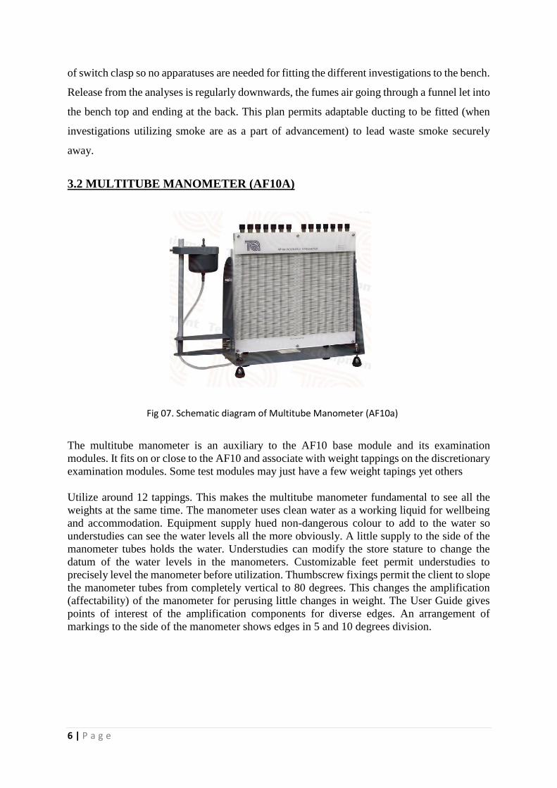
3.2 MULTITUBE MANOMETER (AF10A)

Fig 07. Schematic diagram of Multitube Manometer (AF10a)

The multitube manometer is an auxiliary to the AF10 base module and its examination

modules. It fits on or close to the AF10 and associate with weight tappings on the discretionary

examination modules. Some test modules may just have a few weight tapings yet others

Utilize around 12 tappings. This makes the multitube manometer fundamental to see all the

weights at the same time. The manometer uses clean water as a working liquid for wellbeing

and accommodation. Equipment supply hued non-dangerous colour to add to the water so

understudies can see the water levels all the more obviously. A little supply to the side of the

manometer tubes holds the water. Understudies can modify the store stature to change the

datum of the water levels in the manometers. Customizable feet permit understudies to

precisely level the manometer before utilization. Thumbscrew fixings permit the client to slope

the manometer tubes from completely vertical to 80 degrees. This changes the amplification

(affectability) of the manometer for perusing little changes in weight. The User Guide gives

points of interest of the amplification components for diverse edges. An arrangement of

markings to the side of the manometer shows edges in 5 and 10 degrees division.

7 | P a g e

3.3 Boundary layer Apparatus AF14 (Apparatus used for experiment)

A flat plate is placed in the l00mm x 50mm transparent working section so that a boundary

layer forms along it. A sensitive, wedge shaped pitot tube mounted in a micrometer traverse

allows velocity measurements to be made in the boundary layer. Both laminar and turbulent

layers may be formed. Experiments which may be carried out include the measurement of the

velocity profile:

1. In laminar and turbulent boundary layers.

2. In the boundary layer on rough and smooth plates.

3. In the boundary layer at various distances from the leading edge of the plate.

4. In the boundary layer on plates subject to an increasing or decreasing pressure gradient in

the direction of flow (using the removable duct liners supplied).

3.4 Dimensions and Weights

AF10

Measurement Nett: 1100 x 1000 x 2210mm;

Weight: 120kg Gross: 2.43m3; 260kg.

AF14

Measurement: 0.2 cubic meter

Weight: 10 Kg

8 | P a g e

CHAPTER IV: TEST PROCEDURE

1. The figure gives the plan of the test segment appended to the outlet of

Compression of the airflow bench.

2. A flat plate is placed at the mid height of the section, with a sharpened edge

facing the oncoming flow. Once side of the plate is smooth and the other is rough so

that by turning the plate over, results may be obtained on both types of surfaces.

3. A fine pitot tube may be crossed through the boundary layer at a segment close

the downstream edge of the plate. This tube is extremely fragile instrument which

should be taken care of with compelling consideration if harm is to be stayed away

from. The end of the tube is straightened with the goal that it introduces a limited

opening to the flow.

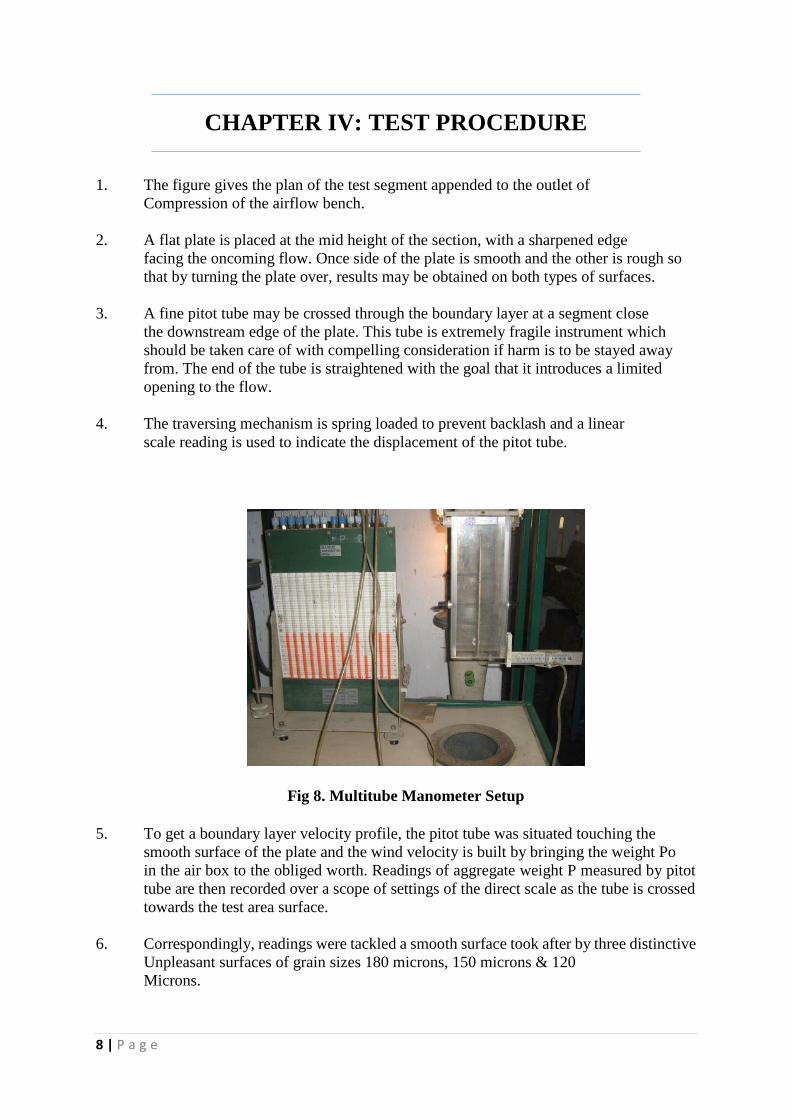
4. The traversing mechanism is spring loaded to prevent backlash and a linear

scale reading is used to indicate the displacement of the pitot tube.

Fig 8. Multitube Manometer Setup

5. To get a boundary layer velocity profile, the pitot tube was situated touching the

smooth surface of the plate and the wind velocity is built by bringing the weight Po

in the air box to the obliged worth. Readings of aggregate weight P measured by pitot

tube are then recorded over a scope of settings of the direct scale as the tube is crossed

towards the test area surface.

6. Correspondingly, readings were tackled a smooth surface took after by three distinctive

Unpleasant surfaces of grain sizes 180 microns, 150 microns & 120

Microns.

9 | P a g e

CHAPTER V: OBSERVATION AND

CALCULATION

1. At first the reading increased constantly along a certain length indicating that

the traverse has been in the boundary layer region. Reading were taken at an interval

of 1mm till the readings reaches to a constant value for a certain length along the

section.

2. On further movement of pitot tube , the readings regularly decreased , indicating that

the pitot tube has entered in the boundary layer region of the test section.

Similarly, readings at different velocities and then for the rough surfaces were

taken.

Damping would have been provided by squeezing the connecting plastic tube but,it

could lead to false readings. So, the unsteady readings were observed and then their

mid reading were taken by us.

Fig 9. Test Apparatus (pitot tube , Multimeter Manometer)

10 | P a g e

3. Rough Section : The Apparatus of Flat Plate is attached with sand paper of roughness

of different size . The figure shows the roughness and smooth plate which was used in

the experiment.

4. Smooth Plate : This Section is made up of aluminium sheet which was used in the

experiment one side edge is sharpened .

Fig 10. Rough Plate Fig 11 Smooth Plate

11 | P a g e

5.1 EXPERIMENTAL DATA and ANAYLYSIS

• Length of plate, L= 0.25m.

• Thickness of pitot tube at tip, 2t=0.4mm.

• So, Movement of tube centre from surface when in contact, t=0.2mm.

• Values of u/U are found from equation given below: (u/U) = √(Pt/Po) Where Pt is Pitot

Pressure and Po is the pitot tube reading in the free stream.

• The Free Stream Velocity is then obtained by the equation given below: (1/2)ρU 2 =Po.

• The Reynold Number is then obtained by the equation given below: Re = UL/ν

• Air Density = 1.151 kg / m3

• Kinematic Viscosity (ν) = 1.49x10-5

ρ Air density

u Velocity at sections

U Free stream velocity

ʋ Kinematic viscosity

μ Dynamic viscosity

ΔP Pressure difference

L Length of the plate

y Distance from the surface

Re Reynolds number

x Distance from the leading edge

ᵟ Boundary thickness

Table -1 Nomenclature symbol

12 | P a g e

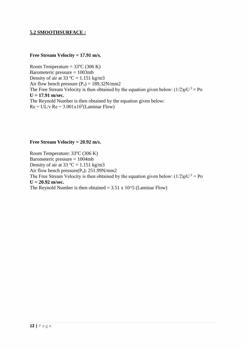
5.2 SMOOTHSURFACE :

Free Stream Velocity = 17.91 m/s.

Room Temperature = 33oC (306 K)

Barometeric pressure = 1003mb

Density of air at 33 oC = 1.151 kg/m3

Air flow bench pressure (Po) = 189.32N/mm2

The Free Stream Velocity is then obtained by the equation given below: (1/2)ρU 2 = Po

U = 17.91 m/sec. The Reynold Number is then obtained by the equation given below:

Re = UL/ν Re = 3.001x105(Laminar Flow)


Room Temperature: 33oC (306 K)



Air flow bench pressure(Po): 251.99N/mm2


U = 20.92 m/sec. The Reynold Number is then obtained = 3.51 x 10^5 (Laminar Flow)

13 | P a g e

Readings for Smooth Plate :

\

Smooth Surface 1 Po=189.32N/mm2 , U=17.91m/s

Table -2

Smooth Surface 2 Po=251.99 N/mm2 , U=20.92m/s

Table 3

Manometer Reading Y (mm) Pt N/mm2 u/U=√

𝑷t

𝑷𝒐

9.2 0.2 122.66 0.70

9.8 1.2 130.66 0.73

10.6 2.2 141.32 0.79

11.4 3.2 151.99 0.84

12.6 4.2 167.99 0.91

13.8 5.2 183.99 0.98

14.0 6.2 186.66 0.99

14.2 7.2 189.32 1

14.2 8.2 189.32 1


𝑷t

𝑷𝒐

13.6 0.2 181.32 0.74

14.2 1.2 189.32 0.78

14.8 2.2 197.32 0.82

15.4 3.2 205.32 0.85

16.6 4.2 221.32 0.86

17.2 5.2 229.32 0.91

18.0 6.2 239.99 0.96

18.8 7.2 250.66 0.99

13.6 0.2 181.32 0.74

14 | P a g e

Fig 12 Velocity Distribution Graph (smooth Plate)

15 | P a g e

5.3 Ansys (Computational Data and Graph)

ANSYS Fluent

ANSYS Fluent software contains the broad physical modeling capabilities needed to model

flow, turbulence, heat transfer, and reactions for industrial applications ranging from air flow

over an aircraft wing to combustion in a furnace, from bubble columns to oil platforms, from

blood flow to semiconductor manufacturing, and from clean room design to wastewater

treatment plants. Special models that give the software the ability to model in-cylinder

combustion, aeroacoustics, turbomachinery, and multiphase systems have served to broaden

its reach.

Today, thousands of companies throughout the world benefit from the use of ANSYS

Fluent software as an integral part of the design and optimization phases of their product

development. Advanced solver technology provides fast, accurate CFD results, flexible

moving and deforming meshes, and superior parallel scalability. User-defined functions allow

the implementation of new user models and the extensive customization of existing ones. The

interactive solver setup, solution and post-processing capabilities of ANSYS Fluent make it

easy to pause a calculation, examine results with integrated post-processing, change any

setting, and then continue the calculation within a single application. Case and data files can

be read into ANSYS CFD-Post for further analysis with advanced post-processing tools and

side-by-side comparison of different cases.

The integration of ANSYS Fluent into ANSYS Workbench provides users with superior bi-

directional connections to all major CAD systems, powerful geometry modification and

creation with ANSYS DesignModeler technology, and advanced meshing technologies in

ANSYS Meshing. The platform also allows data and results to be shared between

applications using an easy drag-and-drop transfer, for example, to use a fluid flow solution in

the definition of a boundary load of a subsequent structural mechanics simulation.

Steps to do Computational Data and Graph in ansys :

1. Geometry

2. Mesh

3. Setup

4. Results

5. Graph

http://www.ansys.com/Products/Simulation+Technology/Fluid+Dynamics/Results+Analysis+Products/ANSYS+CFD-Post

http://www.ansys.com/Products/Workflow+Technology/ANSYS+Workbench+Platform

http://www.ansys.com/Products/Workflow+Technology/ANSYS+Workbench+Platform/ANSYS+DesignModeler

http://www.ansys.com/Products/Workflow+Technology/ANSYS+Workbench+Platform/ANSYS+Meshing

http://www.ansys.com/staticassets/ANSYS/staticassets/product/fluent-product-1-bg.jpg



16 | P a g e

1. Geometry : This is a 3-d Geometry which was same as experimental apparataus and is

used for computational graph. A smooth Plate is attached in between the wall surface

and flow will be given after doing meshing . Meshing is an important part of Ansys

and is having a great importance. Without meshing graph plots cannot be done .

Fig 13. Geometry (Setup Apparatus)

2. Setup : The free stream Velocity is taken as 17.94m/s and density of fluid flowing is

1.151 kg/m3 . The plotting was done . Velocity Distribution graph is shown in the

figure.

Fig 14. Velocity Distribution graph using Ansys.

17 | P a g e

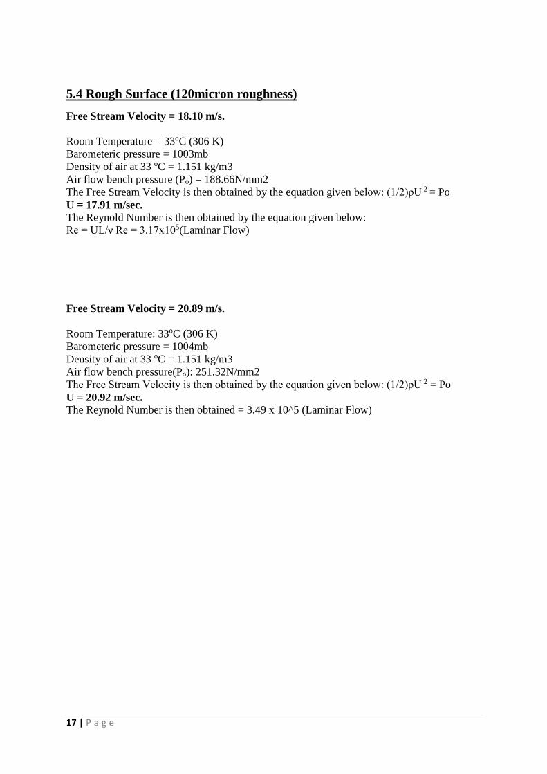
5.4 Rough Surface (120micron roughness)





Air flow bench pressure (Po) = 188.66N/mm2










U = 20.92 m/sec. The Reynold Number is then obtained = 3.49 x 10^5 (Laminar Flow)

18 | P a g e

Readings from 120 Micron Grain Size Sand Paper for Roughness

Rough Surface 120 micron Po=188.66N/mm2 , U=18.10m/s

Table 4


Table 5


𝑷t

𝑷𝒐

11.6 0.2 132.66 0.73

12.2 1.2 151.66 0.75

12.8 2.2 159.72 0.77

13.4 3.2 164.66 0.81

14.2 4.2 171.66 0.84

14.8 5.2 178.43 0.87

15.4 6.2 181.81 0.94

16.0 7.2 186.66 0.98

16.4 8.2 188.66 1


𝑷t

𝑷𝒐

12.6 0.2 162.66 0.70

13.2 1.2 176.32 0.73

13.8 2.2 183.99 0.76

14.4 3.2 191.99 0.77

15.0 4.2 203.19 0.83

15.6 5.2 217.99 0.87

16.2 6.2 227.99 0.95

16.6 7.2 241.32 0.98

17.0 8.2 251.32 1

19 | P a g e

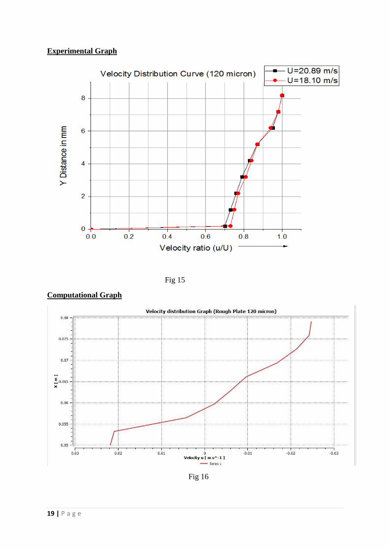
Experimental Graph

Fig 15

Computational Graph

Fig 16

20 | P a g e






Air flow bench pressure (Po) = 198.54 N/mm2




Free Stream Velocity = 20.77m/s.






U = 20.92 m/sec. The Reynold Number is then obtained = 3.48 x 105 (Laminar Flow)

21 | P a g e


Rough Surface 150 micron Po=198.54 N/mm2 , U=18.57m/s

Table 6

Rough Surface 150 micron Po=248.73 N/mm2 , U=20.77m/s

Table 7


𝑷t

𝑷𝒐

11.8 0.2 157.32 0.79

12.4 1.2 161.12 0.81

12.8 2.2 165.32 0.84

13.2 3.2 169.99 0.86

13.6 4.2 172.99 0.91

14.4 5.2 181.32 0.94

15.0 6.2 187.52 0.97

15.2 7.2 198.54 1


𝑷t

𝑷𝒐

12.4 0.2 159.86 0.69

13.2 1.2 176.89 0.74

13.8 2.2 183.99 0.77

14.4 3.2 191.99 0.81

15.0 4.2 199.99 0.85

15.8 5.2 203.99 0.88

16.4 6.2 210.42 0.94

16.8 7.2 231.66 0.96

16.9 8..2 248.73 0.98

22 | P a g e

Fig 17

23 | P a g e






Air flow bench pressure (Po) = 187.66 N/mm2




Free Stream Velocity = 20.16m/s.






U = 20.92 m/sec. The Reynold Number is then obtained = 3.74 x 105(Laminar Flow)

24 | P a g e



Table 8


Table 9


𝑷t

𝑷𝒐

12.2 0.2 144.66 0.75

12.8 1.2 152.96 0.78

13.6 2.2 166.99 0.84

14.2 3.2 171.66 0.86

14.4 4.2 176.66 0.91

14.6 5.2 181.88 0.97

15.0 6.2 185.99 0.99

15.2 7.2 187.66 1


𝑷t

𝑷𝒐

11.6 0.2 154.66 0.71

12.2 1.2 167.66 0.75

12.9 2.2 171.99 0.79

13.6 3.2 181.32 0.81

14.0 4.2 186.66 0.85

14.6 5.2 194.66 0.87

15.2 6.2 202.66 0.93

15.8 7.2 210.66 0.94

16.6 8.2 229.94 0.99

16.8 9.2 233.99 1

25 | P a g e

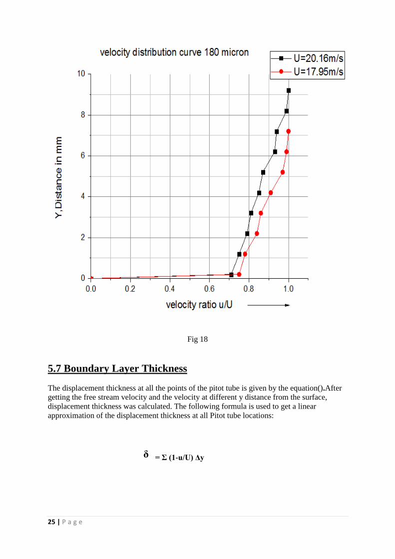
Fig 18

5.7 Boundary Layer Thickness

The displacement thickness at all the points of the pitot tube is given by the equation().After

getting the free stream velocity and the velocity at different y distance from the surface,

displacement thickness was calculated. The following formula is used to get a linear

approximation of the displacement thickness at all Pitot tube locations:

ᵟ = Σ (1-u/U) Δy

26 | P a g e

BOUNDARY LAYER GROWTH

Table . 10 Boundary Layer Thickness

Fig 19 . Growth of Boundary Layer on Smooth and Rough Surface

Types Of Surface Boundary Layer Thickness (mm)

Smooth Surface 0.5835

120 microns 0.6215

150 microns 0.6664

180 microns 0.7150

27 | P a g e

CHAPTER VI: DISCUSSION

1. The Reynolds number shows that the flow is only laminar (Re>500,000) The

Reynolds number is largely a function of speed, viscosity and density of the

fluid.

2. The boundary layer thickness is in the range of 0.4 to 0.8 mm, which was

expected for the air flow bench apparatus.

3. The thickness increases along the surface and roughness increases.

4. The graph shows the boundary layer thickness v/s length of the plate which

give a clear idea of the boundary layer growth along the smooth plate and rough

surfaces of different grain size.

28 | P a g e

CHAPTER VI: CONCLUSION

• The Reynold number so obtained ranges is less than 5 x 10 5 . It

concludes that the velocity distribution observed is in the Laminar

Boundary Layer.

• Also it has been found that reduction in velocity increases with the

increase in free stream velocity.

• The Boundary Layer growth increases as the grain size increases and it

lies between 0.4mm to 0.8 mm.

• Velcoity distribution graph shows how the velocity increase and attains

upto 99 percent of its free stream velocity.

29 | P a g e

CHAPTER VI: REFERENCES

1. A First course in Air Flow by E.Markland

TECQUIPMENT Publishers Lt d .

1 Ma r c h 19 76 .

2. Boundary Layer Transition effected by surface roughness and Free Stream

Turbulence by S.K . Robert and M .I .Yaras. Journal of Fluid Engineering Volume

124 , Issue 3 May 2005.

3. Fluid Mechanics and Fluid Power Engineering by Dr. D.S. Kumar . Katson

Publishing House Delhi . 1999.

4. • Hydraulic and fluid mechanics including hydraulic machines by DR. P.N.MODI and

DR. S.M.SETH.

5. • Kay Gemba, California state university, Long Beach, Measurement of boundary

layer on a Flat plate.

6. • Boundary Layer Transition effected by surface roughness and Free Stream

Turbulence b y S.K. Roberts and M.I.Yaras . Journal of Fluid Engineering Volume

124 , Issue3 Ma y 2005 .

Web Re f e r e n c e s :

www. s c i e n c e di r e c t . c om www.wiki p ed i a . c om

www. en gin e e r i ngt o ol box . com

Date post:	17-Mar-2020
Category:	Documents
Upload:	others
View:	2 times
Download:	0 times

GROWTH OF BOUNDARY LAYER ON SMOOTH AND ROUGH … · 2017-04-18 · In Fluid flow, the Reynolds...

Documents