Growth of structure in the Szekeres class-II inhomogeneous cosmologicalmodels and the matter-dominated era

Mustapha Ishak* and Austin Peel

Department of Physics, The University of Texas at Dallas, Richardson, Texas 75083, USA(Received 18 April 2011; revised manuscript received 23 December 2011; published 3 April 2012)

This study belongs to a series devoted to using the Szekeres inhomogeneous models in order to develop

a theoretical framework where cosmological observations can be investigated with a wider range of

possible interpretations. While our previous work addressed the question of cosmological distances versus

redshift in these models, the current study is a start at looking into the growth rate of large-scale structure.

The Szekeres models are exact solutions to Einstein’s equations that were originally derived with no

symmetries. We use here a formulation of the Szekeres models that is due to Goode and Wainwright, who

considered the models as exact perturbations of a Friedmann-Lemaıtre-Robertson-Walker (FLRW)

background. Using the Raychaudhuri equation we write, for the two classes of the models, exact growth

equations in terms of the under/overdensity and measurable cosmological parameters. The new equations

in the overdensity split into two informative parts. The first part, while exact, is identical to the growth

equation in the usual linearly perturbed FLRW models, while the second part constitutes exact nonlinear

perturbations. We integrate numerically the full exact growth rate equations for the flat and curved cases.

We find that for the matter-dominated cosmic era, the Szekeres growth rate is up to a factor of three to five

stronger than the usual linearly perturbed FLRW cases, reflecting the effect of exact Szekeres nonlinear

perturbations. We also find that the Szekeres growth rate with an Einstein-de Sitter background is stronger

than that of the well-known nonlinear spherical collapse model, and the difference between the two

increases with time. This highlights the distinction when we use general inhomogeneous models where

shear and a tidal gravitational field are present and contribute to the gravitational clustering. Additionally,

it is worth observing that the enhancement of the growth found in the Szekeres models during the matter-

dominated era could suggest a substitute to the argument that dark matter is needed when using FLRW

models to explain the enhanced growth and resulting large-scale structures that we observe today.

DOI: 10.1103/PhysRevD.85.083502 PACS numbers: 98.80.Jk, 95.30.Sf, 98.80.Es

I. INTRODUCTION

Our modern era of cosmology has led to not only awealth of astronomical observations, but also to two majorconundrums, namely, dark matter and dark energy. It istherefore essential to explore theoretical frameworks thatallow for a wider range of possible interpretations of thecosmological data.

Such a framework can be provided by inhomogeneouscosmological models that are exact solutions to Einstein’sequations. A good deal of theoretical work has been doneon such models in the exact theory of general relativity, butlittle work has been done to compare them to observations.This is not surprising, since it is not straightforward inthese models to derive observable functions ready to becompared to cosmological data. See, for example, [1–18],and references therein.

This study is part of a series where we consider theSzekeres inhomogeneous models in order to develop aframework in which to analyze current and future cosmo-logical observations. The models were originally derivedby Szekeres in [19,20] as an exact solution with a generalmetric that has no symmetries and has an irrotational dust

source. The models are regarded as the best exact solutioncandidates to represent the true lumpy Universe we live in.For example, the models are put in the same classificationas the observed lumpy Universe in [21]. The models havebeen investigated analytically and numerically by severalauthors, see, for example, [5,16,22–28,30–37].Any cosmological model must pass at least two types of

cosmological tests. The first is related to measurements ofthe expansion history and cosmological distances, and thesecond is related to measurements of the growth rate ofstructure formation. In previous studies [16,36], we ex-plored distances versus redshift in the Szekeres models,while the current work looks into the growth of structure.In this paper, we study the growth rate of structure in flat

and curved cases of Class-I and Class-II Szekeres modelsusing a reformulation of the models that was introducedby Goode and Wainwright [25,26], where the models canbe considered as nonlinear exact perturbations of theFriedmann-Lemaıtre-Robertson-Walker (FLRW) back-ground. This formulation is well-suited for the study ofthe growth and structure formation in these models. Thework of Ref. [38] extended the flat case of Class-II in [25]to include a cosmological constant and a discussion of thegrowth. Our work here extends that of [25] to spatiallycurved cases in Class-I and Class-II in analyzing the*mishak@utdallas.edu

PHYSICAL REVIEW D 85, 083502 (2012)

1550-7998=2012=85(8)=083502(14) 083502-1 2012 American Physical Society

growth. We also express the growth differential equationsas well as equations for the shear and tidal gravitationalfield, all in terms of the under/overdensity and measurablecosmological parameters, which offer further insights overthe metric functions themselves. We analyze the timeevolution of the growth factor, shear, and tidal gravitationalfield scalars in flat and curved cases and discuss theirinterrelationship via the propagation equations to producestronger gravitational clustering in Szekeres models.

The paper is organized as follows. After presentingthe formalism in Sec. II, we show in Sec. III how theRaychaudhuri propagation equation gives exact nonlineargrowth equations in terms of the under/overdensity thatdivide into two meaningful parts. We express these equa-tions for the flat and curved cases of Class-II in terms ofgrowth factor, the scale factor, and measurable cosmologi-cal parameters. We perform numerical integrations of thesenew equations and plot the results for various cases. Theresults are also compared to those of the linearly perturbedEinstein-de Sitter model and the nonlinear spherical col-lapse. In Sec. IV we repeat the analysis for models ofClass-I. We then explore the shear and the tidal gravita-tional field and their relation to the growth in Sec. V. Weconclude in Sec. VI. Throughout the paper, we use unitssuch that 8G ¼ c ¼ 1.

II. THE SZEKERESMODELS IN THE GOODE ANDWAINWRIGHT REPRESENTATION

Since the original derivation of the models by Szekeresin [19,20], they have been reformulated in at least twoother different sets of coordinates. The second formulationwas proposed by Goode and Wainwright [25,26], and athird set was used in e.g. [4,37]. The relationships betweenthese formulations can be found in [2,26,37]. As men-tioned earlier, we chose in this study to use the representa-tion of Goode and Wainwright because it is well-suited forthe study of the growth of structure and exact perturbationsof a smooth FLRW background. In order to be self-contained, we repeat and summarize here the presentationof the models in the Goode and Wainwright presentation[some typos have been fixed from their original paper].This also serves to set the notation to be used in the paper.The Szekeres metric in the Goode and Wainwright set ofcoordinates ft; x; y; zg reads

ds2 ¼ dt2 þ S2½e2ðdx2 þ dy2Þ þH2W2dz2; (1)

where

Hðt; x; y; zÞ ¼ Aðx; y; zÞ Fðt; zÞ¼ Aðx; y; zÞ ðþfþ þ fÞ (2)

andHðt; x; y; zÞ, Sðt; zÞ, andWðzÞ are all positive functions.þ and are functions of z only, and fþ and f arefunctions of t and z. Aðx; y; zÞ and ðx; y; zÞ will be furtherspecified below.

The source of the spacetime is irrotational dust, and thecoordinates are comoving and synchronous. The cosmicdust fluid thus has the 4-velocity vector ua ¼ ½1; 0; 0; 0.The two classes of solutions are listed below with further

specifications of the functions for each class. The functionSðt; zÞ satisfies the generalized Friedmann equation

_S 2 ¼ kþ 2M

S; (3)

where _¼ @=@t,M ¼ MðzÞ, and k ¼ 0,1. Next, it can beverified that the functions fþ and f (see Eqs. (8) and (9)below) are the increasing and decreasing solutions of thefollowing ordinary differential equation [26]:

€Fþ 2_S

S_F 3M

S3F ¼ 0; (4)

which can be derived from the field equations as well asfrom the Raychaudhuri equation that we discuss further inthe following section.Interestingly, the time evolution of the two spatial

classes of the models is fully described by the same twoequations (3) and (4). Equation (3) reduces to the usualFriedmann equation for a fixed z while Eq. (4) governsdensity fluctuations.The matter density in the models is given by

ðt; x; y; zÞ ¼ 6M

S3

1þ F

H

¼ 6MA

S3H: (5)

In this formulation, the vanishing of the functions þand is the necessary and sufficient condition for themodels to reduce to FLRWmodels. In this limit, the sign ofthe matter density is determined by that of MðzÞ, and thuswe shall limit our interest to models with MðzÞ> 0.

A. Time dependence

The time dependence of the models is specified by theparametric and implicit solutions for the functions Sðt; zÞ,fþðt; zÞ, and fðt; zÞ from Eqs. (3) and (4). The solution ofthe generalized Friedmann equation (3) is given in para-metric form using as

S ¼ MdhðÞd

with t TðzÞ ¼ MhðÞ; (6)

where

hðÞ ¼8><>: sin k ¼ þ1

sinh k ¼ 1

3=6 k ¼ 0

: (7)

(Note that MðzÞ> 0 is required in all cases, and whenk ¼ 0 or k ¼ 1 then we require that _S > 0.) So the scalefunction S has the same time dependence as that of anFLRW dust model. Next, the solution to Eq. (4) gives

MUSTAPHA ISHAK AND AUSTIN PEEL PHYSICAL REVIEW D 85, 083502 (2012)

083502-2

fþ ¼8><>:ð6M=SÞ½1 ð=2Þ cotð=2Þ 1 k ¼ þ1

ð6M=SÞ½1 ð=2Þ cothð=2Þ þ 1 k ¼ 1

2=10 k ¼ 0

(8)

f ¼8><>:ð6M=SÞ cotð=2Þ k ¼ þ1

ð6M=SÞ cothð=2Þ k ¼ 1

24=3 k ¼ 0

: (9)

B. Spatial dependence

The spatial dependence of the models separates theminto two classes. Class I:

S ¼ Sðt; zÞ; Sz 0; f ¼ fðt; zÞ;T ¼ TðzÞ; M ¼ MðzÞ

with

e¼fðzÞ½aðzÞðx2þy2Þþ2bðzÞxþ2cðzÞyþdðzÞ1; (10)

ad b2 c2 ¼ =4; ¼ 0;1;

A ¼ fz kþ; W2 ¼ ð kf2Þ1;

þ ¼ kfMz=ð3MÞ; ¼ fTz=ð6MÞ;(11)

where the subscript z in the equations means differentiationwith respect to z. Class-II:

S ¼ SðtÞ; f ¼ fðtÞ;T ¼ const; M ¼ const

with

e ¼ ½1þ k=4ðx2 þ y2Þ1; k ¼ 0;1; W ¼ 1;

(12)

A ¼8><>:eaðzÞ

1 k

4 ðx2 þ y2Þþ bðzÞxþ cðzÞy

kþ; k ¼ 1

aðzÞ þ bðzÞxþ cðzÞy þðx2 þ y2Þ=2; k ¼ 0: (13)

C. Raychaudhuri equation and gravitational attraction

The complete dynamics of a cosmological model can beexpressed in terms of a set of evolution and propagationequations (see, for example, [21,39] and citations, therein).One of the fundamental propagation equations is theRaychaudhuri equation [40], and it can be viewed as thebasic equation of gravitational attraction [21]. In the caseof the Szekeres irrotational dust, the equation reads

_þ 13

2 þ 22 þ 12 ¼ 0; (14)

which includes the following quantities associated with the4-velocity vector ua listed as follows (a semicolon denotescovariant differentiation and parentheses around indicesindicate symmetrization):

(i) the rate of volume expansion scalar

ua;a ¼ 3_S

S _F

H(15)

(ii) the rate of shear tensor

ab uða;bÞ þ _uðaubÞ

3ðgab þ uaubÞ; (16)

where for our models the corresponding nonzerocomponents are

2xx ¼ 2y

y ¼ zz ¼ 2

3

_F

H(17)

(iii) and the matter density , which is given by Eq. (5).

For a complete Raychaudhuri equation including pres-sure, vorticity, 4-acceleration, and a cosmological constant(all zero in our models here) see, for example, [21,39].Now, using Eqs. (15) and (17), the generalized

Friedmann equation (3) (making the appropriate substitu-tion for €S), and the density equation (5), we can write theRaychaudhuri equation (14) as second-order ordinary dif-ferential equation that is linear in the function F:

€Fþ 2_S

S_F 3M

S3F ¼ 0: (18)

As pointed out in [26], this differential equation of themetric function F derives from the field equations as wellas the Raychaudhuri equation. However, as we will explorein the rest of the paper, associating this equation with themeaning of the Raychaudhuri equation and that of otherevolution equations involving shear and tidal gravitationalfields will help us build a consistent discussion of gravita-tional clustering in the Szekeres models.Including the previous section, all equations up to this

point apply generally to both Class-I and Class-II of theSzekeres models. However in the following sections, weneed to treat the discussion of the growth equations forClass-I and Class-II separately in view of their differentspatial dependencies.

III. STRUCTURE GROWTH EXACT EQUATIONSIN SZEKERES CLASS-II MODELS

We start by exploring Class-II first because of its simplerspatial dependence. In this case, the function SðtÞ is only afunction of t while M and T are constants. The connection

GROWTH OF STRUCTURE IN THE SZEKERES CLASS-II . . . PHYSICAL REVIEW D 85, 083502 (2012)

083502-3

to the growth of large-scale structure is simpler since inEqs. (19) and (20) below is only a function of t.

Now we define, in the usual way, the density contrast as

ðt; x; y; zÞ ðt; x; y; zÞ ðtÞðtÞ (19)

so that we can write

ðt; x; y; zÞ ¼ ðtÞ½1þ ðt; x; y; zÞ: (20)

Comparing Eqs. (20) and (5) specialized to Class-II that is

ðtÞ ¼ 6M

SðtÞ3 ; (21)

which is a function of t only. Since M is constant, weidentify immediately

ðt; x; y; xÞ ¼ F

H: (22)

Using the relations _F ¼ _H þ _H and €F ¼€H þ 2 _ _Hþ €H obtained from Eq. (22), theRaychaudhuri equation (18) becomes

€H þ 2 _ _Hþ €H þ 2_S

Sð _H þ _HÞ 3

M

S3H ¼ 0:

(23)

Noting that _H ¼ _F and €H ¼ €F, we can rewrite theabove equation (divided by H) as

€þ 2_H

H_ 3

M

S32 þ 2

_S

S_ 3

M

S3 ¼ 0: (24)

We can eliminate _H=H with the above relation for _F andarrive at the following exact growth equation for theSzekeres Class-II models:

€þ 2_SðtÞSðtÞ

_ 3M

SðtÞ3 2

1þ _2 3

M

SðtÞ3 2 ¼ 0:

(25)

Now, we use the same idea of Goode and Wainwright[25,26], who stated that the Szekeres models in their for-mulation allows one to compare them with linear pertur-bations of the FLRW models [25]. Additionally, asexplained in [26], the function Sðt; zÞ in the generalizedFriedmann equation (3) corresponds to the scale factor inthe FLRW models in the sense that for each value of z itsatisfies the Friedmann equation. In other words, for eachSzekeres model explored, we associate a correspondinglinearly perturbed FLRW model. The exact growth equa-tion obtained from the Szekeres model is then compared tothe linearly perturbed associated FLRW model. The un-perturbed FLRW model is called here and in other papersthe associated FLRW background. It is worth clarifyingthat this association is not based on the usual procedure ofimposing certain limits on coordinates or somehow

restricting the metric functions such that the Szekeresmodel reduces to a FLRW model [2], even if theSzekeres model may be related to it.So following [25,26], we associate the Szekeres models

to nonlinear exact perturbations of an associated FLRWbackground, and we write here the growth Eq. (25) withan exact density contrast as perturbations of an FLRWmodel with the corresponding Hubble function and matterdensity as given below in Eqs. (27) and (28). The equationthen reads

€þ 2HðtÞFLRWB_ 4GðtÞFLRWB

2

1þ _2 4GðtÞFLRWB

2 ¼ 0; (26)

where we have identified the Hubble expansion rate of theFLRW background (FLRW-B)

H ðtÞFLRWB _SðtÞSðtÞ : (27)

Note that this HðtÞ is not the same function as the metricfunctionHðt; x; y; zÞ. SinceM is a constant in Class-II here,we have used Eq. (5) to express the factor 3M

S3in terms of the

smooth background matter density as

3M

SðtÞ3 ¼ 4GðtÞFLRWB: (28)

Note that while throughout this treatment we set ¼8G ¼ 1, we restored its value here to make identificationwith the usual FLRWexpressions immediate.It is also worth noting that the Raychaudhuri propaga-

tion equation provided us with an exact equation for thegrowth function that can be remarkably split into twomeaningful parts. One part, which consists of the first threeterms, is identical to the usual equation of growth for alinearly perturbed FLRW model. The other part contains

the remaining nonlinear terms in and _ and is similar tosecond-order perturbation terms. But we note here that ourequation is exact, and does not have to be small. In thenext subsections, we specialize the exact growth rateEq. (25) of the Szekeres Class-II to the flat and curvedcases and then integrate them numerically.

A. Growth rate equations and integration in flatSzekeres Class-II models

In this case, the corresponding FLRW background isthus the well-known Einstein-de Sitter model that is ap-propriate for describing the matter-dominated phase ofcosmic evolution. For an Einstein-de Sitter background,the scale factor can be solved from Eq. (3) as

SðtÞ ¼9

2M

1=3

t2=3 ¼ t2=3; (29)

where for k ¼ 0 we can set M ¼ 2=9 in all generality (forexample, see [26]). Using Eq. (29) in Eqs. (26) or (25)yields

MUSTAPHA ISHAK AND AUSTIN PEEL PHYSICAL REVIEW D 85, 083502 (2012)

083502-4

€þ 4

3t_ 2

3t2 2

1þ _2 2

3t22 ¼ 0: (30)

We note again that the first three terms are exactly thesame as the ones in the usual linearly perturbed Einstein-de Sitter case, so this could be identified with the lineartheory when is small. The second part is made of two

nonlinear terms in _ and and can be compared to second-order perturbation terms [41].

The full equation obtained can be compared as well tothe spherical nonlinear collapse model, which is given inEqs. (35) and (36). As in the case of nonlinear sphericalcollapse [41] for Einstein-de Sitter, a parametric solution iswell-known (see, for example, [42]) but we found it morepractical for our cosmology numerical codes to performthe integrations numerically. Moreover, the numerical in-tegration schemes are expandable to cases where para-metric solutions are not known.

Next, we write the growth rate Eq. (30) in terms of thescale factor. To convert time derivatives to S derivatives,we first note that

_ ¼ 2

3S1=20 (31)

and

€ ¼ 4

9S0 2

9S200; (32)

where primes denote derivatives with respect to S. Here,and throughout the rest of the paper, we write aðtÞ for thescale factor SðtÞ by analogy with FLRWmodels, and take itto have the standard normalization aðt0Þ ¼ 1 today. Wethus obtain

00 þ 3

2

0

a 3

2

a2 2

1þ 02 3

2

2

a2¼ 0: (33)

For our numerical integrations, we write the growth equa-tion in terms of the growth rate G =a. Using therelations 0 ¼ Gþ aG0 and 00 ¼ aG00 þ 2G0, we get

G00 þ 7

2

G0

a 2

a

ðGþ aG0Þ21þ aG

3

2

G2

a¼ 0: (34)

We integrate this equation using a fourth-order Runge-Kutta algorithm with adaptive step size [43]. We imple-ment the Runge-Kutta code with the function vectors y ¼fG;G0g and dy

da ¼ fG0; G00g [43] so that the second-order

ordinary differential equation (ODE) (34) is reduced totwo first-order ODEs that are immediately integrable.Our results for the integration are given in the left part of

Fig. 1. The horizontal line G ¼ 1 corresponds to the line-arly perturbed Einstein-de Sitter model, while the redcurve (highest) represents the solution to the full exactgrowth Eq. (34) for the flat Szekeres model of Class-II.The Szekeres growth is up to a factor of 3 stronger than thatof the perturbed Einstein-de Sitter background.For further comparisons, we also integrate numerically

the growth for the well-known nonlinear spherical collapsemodel in an Einstein-de Sitter background (see, for ex-ample, [41]), where the governing equation is given by

00 þ 3

2

0

a 3

2

a2 4

3

1

1þ 02 3

2

2

a2¼ 0 (35)

or in the G-notation

G00 þ 7

2

G0

a 4

3a

ðGþ aG0Þ21þ aG

3

2

G2

a¼ 0: (36)

The resulting integration is also plotted in the left part ofFig. 1. The Szekeres growth is found to be stronger thanthat of the spherical collapse model, as well. Moreover, therelative difference also increases as a function of time.This indicates that the growth rate is different when the

0.5

1

1.5

2

2.5

3

0.1 0.2 0.3 0.4 0.5 0.6

δ/a

a

Szekeres Class-II with an Einstein de Sitter backgroundSpherical Collapse Model in Einstein de Sitter model

FLRW - Einstein de Sitter model

0.5

1

1.5

2

2.5

3

3.5

4

4.5

5

0.1 0.2 0.3 0.4 0.5 0.6

δ/a

a

Szekeres Class-II with ΩMo=1.5

Szekeres Class-II with ΩMo=1.3

Szekeres Class-II with ΩMo=1.2

FLRW with ΩMo=1.5

FLRW with ΩMo=1.3

FLRW with ΩMo=1.2

FLRW - Einstein de Sitter model

0.5

1

1.5

2

2.5

0.1 0.2 0.3 0.4 0.5 0.6

δ/a

a

Szekeres Class-II with ΩMo=0.8

Szekeres Class-II with ΩMo=0.5

Szekeres Class-II with ΩMo=0.3

FLRW with ΩMo=0.8

FLRW with ΩMo=0.5

FLRW with ΩMo=0.3

FLRW - Einstein de Sitter model

FIG. 1 (color online). LEFT: Growth rate of structure in flat Szekeres Class-II models (or Class-I models with a fixed value of z, seeSec. IV) (red, solid curve), the usual spherical collapse model (green, dashed curve), and the perturbed Einstein-de Sitter (EdS) model(blue, dotted line). The Szekeres growth rate is stronger than that of the perturbed EdS by up to a factor of 3. The Szekeres growth rateis also stronger than that of the spherical collapse model. CENTER: Growth rate of structure in positively curved Szekeres Class-IImodels for various values of 0

M (or Class-I models with a fixed value of z and various values of 0MðzÞ). The growth rate in linearly

perturbed FLRWmodels with the same values of0M are plotted for comparison. RIGHT: Growth rate of structure in negatively curved

Szekeres Class-II models for various values of0M (or Class-I models with a fixed value of z and various values of0

MðzÞ). The growthrate in linearly perturbed FLRW models with the same values of 0

M are plotted for comparison, as well. In both cases, the Szekeres

growth rates are stronger than those of the corresponding perturbed FLRW models by up to 5 times.

GROWTH OF STRUCTURE IN THE SZEKERES CLASS-II . . . PHYSICAL REVIEW D 85, 083502 (2012)

083502-5

spherical symmetry approximation for inhomogeneities isnot assumed. As we discuss in Sec. Vand in the concludingremarks, the Szekeres models have shear and tidal gravi-tational fields that contribute to the enhancement of theirgravitational collapse and growth rate.

B. Growth rate equations and integration in curvedSzekeres Class-II models

Now, we derive the growth ODE for the positively andnegatively curved cases (k ¼ 1). Both situations can behandled simultaneously and lead ultimately to the sameequation that we integrate numerically. We begin fromgrowth Eq. (25)

€þ 2_a

a_ 3

M

a3 2

1þ _2 3

M

a32 ¼ 0 (37)

and the generalized Friedmann equation (3)_a

a

2 H2 ¼ 2M

a3 k

a2; (38)

where an overdot denotes differentiation with respect to t(partial in the case of and total for a). We define M 2M=ða3H2Þ and k k=ða2H2Þ by analogy with stan-dard cosmology such that (38) can be written as M þk ¼ 1. We proceed with a more general approach thanfor the flat case that does not require an explicit expressionfor a as a function of t for the different k values. This isaccomplished by using Eq. (38) directly to recast Eq. (37)into integrable form. As before, we convert time deriva-tives to a derivatives via the (now general) relations

_ ¼ @

@t¼ @

@a

da

dt¼ 0 _a (39)

and

€ ¼ @

@tð0 _aÞ ¼ _a200 þ €a0: (40)

Substituting these relations into Eq. (37), we find

00 þ€a

_a2þ 2

a

0 3

M

a3 _a2 2

1þ 02 3

M

a3 _a22 ¼ 0:

(41)

Next we use Eq. (38) to eliminate _a and €a in favor of M

and (implicitly)k. Taking its time derivative and dividingby _a2 gives the coefficient on 0

€a

_a2þ 2

a¼ 4M

2a: (42)

The coefficients on and 2 are also easily converted as

3M

a3 _a2¼ 3

2

M

a2; (43)

and so we obtain the equation

00 þ2MðaÞ

2

0

a 3

2MðaÞ

a2

2

1þ 02 3

2MðaÞ

2

a2¼ 0: (44)

Again, we see that the first part agrees perfectly with theusual growth equation for the spatially curved linearlyperturbed FLRW models [41], while the second part ismade of two nonlinear terms that can be compared tosecond-order perturbation terms. Converting, as before,to G-notation for integration, we obtain

G00 þ4MðaÞ

2

G0

aþ 2ð1MðaÞÞ G

a2

2

a

ðGþ aG0Þ21þ aG

3

2MðaÞG

2

a¼ 0: (45)

We must now express M explicitly in terms of the scalefactor a and the matter density parameter [today] 0

M.Using the definitions of M and k and the Friedmannequation (38) evaluated today, we see that

10M ¼ k

H20

(46)

allows the Friedmann equation (38) at a given time to bewritten as

H 2 ¼ 2M

a3H2

0ð0M 1Þa2

; (47)

where a super- or subscript naught means that the parame-ter is evaluated today. Dividing by H2, (47) becomes

1 ¼ MðaÞ H20ð0

M 1ÞH2a2

; (48)

and dividing (38) by H20 yields

H2

H20

¼ 1

a3½0

M að0M 1Þ: (49)

Thus we find the usual relation

MðaÞ ¼ 0M

0M þ að10

MÞ; (50)

which upon substituting into (45), gives finally

G00 þ4 0

M

2½0M þ að10

MÞG0

a

þ 2

1 0

M

0M þ að10

MÞG

a2 2

a

ðGþ aG0Þ21þ aG

3

2

0

M

0M þ að10

MÞG2

a¼ 0: (51)

It is this equation that we integrate numerically in our codefor various values of 0

M. We note that the same differen-tial Eq. (51) governs both the k ¼ þ1 and the k ¼ 1

MUSTAPHA ISHAK AND AUSTIN PEEL PHYSICAL REVIEW D 85, 083502 (2012)

083502-6

cases. The dependence on k is accounted for in the signof 10

M. As expected, it is clear that setting 0M ¼ 1

indeed recovers the growth equation for the k ¼ 0 casederived in Sec. III A.

Our results for the integration of the curved cases aregiven in Fig. 2 for various values of 0

M and includepositively and negatively curved models. We also integrateand plot the corresponding linearly perturbed FLRW mod-els. As in the spatially flat cases, we find that the curvedSzekeres growth is up to 5 times stronger than that of thelinearly perturbed curved FLRW. Also, some Szekeresmodels with 0

M < 1 can still have a stronger growththan that of the Einstein-de Sitter growth.

In addition to the growth, it is worth plotting the energydensity evolution in order to verify that, after the expectedinitial singularity, it has no other divergences during thematter-dominated era of interest here. We use Eqs. (5) and(20) and some of the steps above to write the energydensity as follows:

¼ 6M

a3ð1þ Þ ¼ 3H2

0

0M

a3ð1þ aGÞ: (52)

Our plots in Fig. 2 for the density as a function of the scalefactor for the flat and curved Szekeres show that the energydensity diverges toward the initial singularity, as it should,and after it decreases monotonically with no other diver-gences during the matter-dominated era plotted here witha 0:35 (i.e., well before a 0:60, which corresponds tothe equality time between matter dominance and cosmo-logical constant dominance in an FLRW-LCDM (Lambda-Cold-Dark-Matter) model; see, for example, [44,45]). Ourfirst goal here is to represent the growth rate during thematter-dominated era with a 0:35, and as the densityplots show, we are far away from any possible pancake

singularity that could occur at later times [26].Additionally, such pancake singularities can be avoidedin some cases by the addition of a cosmological constantto the models [38], although the discussion there waslimited to the flat case. Finally, we conclude in this sectionthat the growth rate of large-scale structure is consistentlyfound to be much stronger in the Szekeres models than inthe linearly perturbed FLRW models with the same matterdensity.

IV. STRUCTUREGROWTHEXACT EQUATIONS INSZEKERES CLASS-I MODELS

A. Flat Szekeres Class-I models

Unlike in the spatially curved Class-I models, the timeevolution Eq. (6) in the flat case can be decoupled and onecan set without loss of generality M ¼ 2=9 [26]. As aresult, the treatment of the growth in the flat case can bedeveloped in exactly the sameway as was done for Class-IIin Sec. III. However, a closer look at Eq. (11) shows that fork ¼ 0 in Class-I þ ¼ 0, so there are no growing modesand this case becomes of no interest for our purpose.

B. Growth rate equations and integration in curvedSzekeres Class-I models

In the spatially curved Class-I models, the functionsSðt; zÞ and MðzÞ are now z-dependent. As a result, theidentification of an under- or overdensity function as wellas a background will require some discussions and defini-tions different from the ones we made for Class-II.

We define a density contrast as

ðt; x; y; zÞ ðt; x; y; zÞ qðt; zÞqðt; zÞ ; (53)

0.10 0.15 0.20 0.25 0.30 0.350

1000

2000

3000

4000

5000

a0.10 0.15 0.20 0.25 0.30 0.350

500

1000

1500

2000

2500

3000

3500

a

10%

5%

Szekeres M0 0.367

0.354

0.340

0.327

EdS

0.1 0.2 0.3 0.4 0.5 0.60.85

0.90

0.95

1.00

1.05

1.10

1.15

a

FIG. 2 (color online). LEFT: Energy density in flat and positively curved Szekeres Class-II models (or Class-I models with a fixedvalue of z, see Sec. IV). The density is plotted as a function of the scale factor well within the matter-dominated cosmological era(a 0:35) (i.e., well before a 0:60, the scale factor associated with matter and cosmological constant equality in the FLRW-LCDMstandard model [44,45]). The density diverges as it should as a tends to the initial singularity, and it decreases monotonically forincreasing a with no further divergences during the matter-dominated era. CENTER: Energy density in negatively curved SzekeresClass-II models (or Class-I models with a fixed value of z). The flat case is also given as reference. The same observations hold here.Further discussion is given in Secs. III and V. RIGHT: Comparisons of some Szekeres models to a growth range band of 5% around theEdS growth, which is also the approximate representation for the FLRW-LCDM model during the matter-dominated era underconsideration. We find that there are Szekeres models that are consistent with such growth range during the cosmological eraconsidered within the 5% range, but the Szekeres models require only about the third of matter energy density than that of the Einstein-de Sitter. This is consistent with our result of stronger structure growth in the Szekeres models.

GROWTH OF STRUCTURE IN THE SZEKERES CLASS-II . . . PHYSICAL REVIEW D 85, 083502 (2012)

083502-7

where we use the quasilocal average density [46–49]

qðt; zÞ ¼Rz

Rx

Ry Fðt; x; y; zÞ ffiffiffiffiffiffiffih

pdzdxdyR

z

Rx

Ry F

ffiffiffiffiffiffiffiffihp

dz dx dy

¼ hiqD½zðtÞ (54)

for the domain D½z delimited by z ¼ constant and con-tained in the hypersurface t ¼ constant. Here h is thedeterminant of the three-dimensional part of the projectiontensor hab ¼ gab þ uaub, and F is a physically mean-ingful weighting function that was discussed in [46–50].

It was shown in [46–49] that q is a coordinate inde-

pendent quantity that can be expressed in terms of curva-ture invariants and is given for the Szekeres Class-I modelsby [49]

qðt; zÞ ¼ 6MðzÞSðt; zÞ3 : (55)

As discussed in [46–48], the term quasilocal follows fromthe integral definition used for the quasilocal Misner-Sharpmass-energy in spherical symmetry [51]. Bearing in mindthatMðzÞ is associated with such a quasilocal mass-energy,the result (55) is not unexpected.

Using the definition (54), we can write

ðt; x; y; zÞ ¼ qðt; zÞ½1þ ðt; x; y; zÞ: (56)

Comparing Eq. (56) and Eq. (5), we identify

ðt; x; y; zÞ ¼ F

H: (57)

Again, using Eq. (57) in the Raychaudhuri equation (18)gives, after a few steps, the following exact growth equa-tion for the Szekeres Class-I models

€þ 2

_Sðt; zÞSðt; zÞ

_ 3

MðzÞSðt; zÞ3 2

1þ

_2 3

MðzÞSðt; zÞ3

2 ¼ 0:

(58)

Next, following a large number of papers using theLemaıtre-Tolman-Bondi models (LTB) for the purpose ofcomparing them to observations (see, for example,[3,9,52,53] and references therein) we can generalizesome definitions from the FLRW models to the Szekeresmodels. We start by rewriting the Szekeres generalizedFriedmann equation (3) as

_Sðt; zÞSðt; zÞ

2 Hðt; zÞ2 ¼ 2MðzÞ

Sðt; zÞ3 k

Sðt; zÞ2 : (59)

We then define

Mðt; zÞ 2MðzÞSðt; zÞ3Hðt; zÞ2 (60)

and

kðt; zÞ k

Sðt; zÞ2Hðt; zÞ2 (61)

by analogy with standard cosmology such that (59) can bewritten as

Mðt; zÞ þkðt; zÞ ¼ 1: (62)

Now, following the same approach we used for Class-IIearlier and the idea introduced by Goode and Wainwright[25,26], we can define a background that is independent of

coordinates x and y, and where the ðt; x; y; zÞ can beregarded as an exact perturbation satisfying the exactequation

€þ 2Hðt; zÞ _ 4Gq 2

1þ

_2 4Gq

2 ¼ 0

(63)

Again, we can observe that this exact growth equationsplits into two meaningful parts. One part, which consistsof the first three terms, is similar to the usual equation ofthe growth for a linearly perturbed FLRWmodel. The other

part consists of the nonlinear terms in and_.

We follow now the steps performed in the curved casesfor Class-II with an overdot here that always denotespartial differentiation with respect to t. We use Eq. (59)to recast Eq. (58) into integrable form. After some stepssimilar to Eqs. (39)–(43) and moving to a-notation, weobtain

00 þ2Mða; zÞ

2

0

a 3

2Mða; zÞ

a2

2

1þ 02 3

2Mða; zÞ

2

a2¼ 0: (64)

It is worth noting again that here a is a function of t and z,while in Class-II it was a function of t only.

Next, converting as before to notation using G =afor integration, we obtain

G00 þ4Mða; zÞ

2

G0

aþ 2ð1Mða; zÞÞ G

a2

2

a

ðGþ aG0Þ21þ aG

3

2Mða; zÞ G

2

a¼ 0: (65)

Now, we can express Mða; zÞ explicitly in terms of thescale factor a and the matter density parameter today0

MðzÞ where a super- or subscript naught means that theparameter is evaluated today. One obtains

Mða; zÞ ¼ 0MðzÞ

0MðzÞ þ að10

MðzÞÞ; (66)

which we substitute into (65) to finally get

MUSTAPHA ISHAK AND AUSTIN PEEL PHYSICAL REVIEW D 85, 083502 (2012)

083502-8

G00 þ4 0

MðzÞ2½0

MðzÞ þ að10MðzÞÞ

G0

a

þ 2

1 0

MðzÞ0

MðzÞ þ að10MðzÞÞ

G

a2 2

a

ðGþ aG0Þ21þ aG

3

2

0

MðzÞ0

MðzÞ þ að10MðzÞÞ

G2

a¼ 0: (67)

We first note that unlike the case of Class-II, here0MðzÞ

has a z-dependence thus in order to perform the plots wewill use it for a fixed value of z. Just as we specified for thequasilocal average density, we use this quasilocal averagedensity number within a domain limited by such a constantvalue of z.

Our results for a fixed value of z are then identical inform to those of Class-II and are plotted and discussed inFigs. 1 and 2. The comments and remarks made for Class-IIapply here as well.

In summary, for both Class-I or Class-II, the Szekeresgrowth is found to be up to 5 times stronger than that of thelinearly perturbed curved FLRW. Also, our plots in Fig. 2for the density as a function of the scale factor for allclasses and the cases that we explored show that the energydensity diverges toward the initial singularity, as it should,and afterward it decreases monotonically with no otherdivergences during the matter-dominated era that we con-sidered in this analysis. In order to explore further thestrong growth found in the Szekeres models, we examinein the next section the shear and gravitational tides in themodels.

V. THE SHEAR AND THE TIDAL GRAVITATIONALFIELD IN SZEKERES MODELS

In this section we analyze the time evolution of furtherphysical quantities that can affect directly or indirectly thegravitational clustering and the growth rate of structure inthe Szekeres models. The source being irrotational dust(i.e. zero vorticity and 4-acceleration), these are the rate ofshear and tidal gravitational field. For this, we considertheir corresponding scalar invariants.

The discussion in this section applies to Class-I andClass-II since the evolution equations and scalar invariantsare common to both classes. The distinction between thetwo treatments is that when we talk about Class-II, we useðt; x; y; zÞ, G =a, M, aðtÞ, and ðaÞ, while we use forClass-I ðt; x; y; zÞ, G =a, MðzÞ, aðt; zÞ, and ða; zÞevaluated at a fixed value of z as defined in the twoprevious sections. For simplicity of notation, we use theformalism as used for Class-II but with observations andconclusions applying as well to Class-I with z fixed.

First we consider a shear scalar that is equal to twice thecommonly used magnitude of the rate of shear [21,39] anddefined as

2 ¼ ab

ba; (68)

where the shear tensor components are given in Eq. (17)(note there is no factor 1=2 in the definition). Computingthis and taking the square root, we find

¼ffiffiffi2

3

s_H

H: (69)

In order to analyze the time evolution of this scalar, weexpress it as a function of the scale factor and currentmeasurable cosmological parameters. We can relate it tothe density contrast via Eq. (22) and by noting that due tothe metric function dependencies, we have _H ¼ _F.Differentiating with respect to time allows us make theidentification

_H

H¼

_

1þ : (70)

Now, using Eq. (39) and converting under/overdensities(s) to growth rates (G’s) as before, we obtain the shear interms of the scale factor and the Hubble parameter H

jj ¼ffiffiffi2

3

sGþ aG0

1þ aGaH: (71)

We use Eq. (49) to rewrite the Hubble parameterH in termsof its measured value today H0 and that of the matterdensity today 0

M

jj ¼ffiffiffi2

3

sGþ aG0

1þ aGH0

ffiffiffiffiffiffiffiffiffiffiffiffiffiffiffiffiffiffiffiffiffiffiffiffiffiffiffiffiffiffiffiffiffiffiffi0

M

a ð0

M 1Þs

: (72)

Along with jj, another related quantity that is worthanalyzing in our models is the shear scalar over the expan-

sion scalar jj . This is particularly useful when looking at

the early time divergences as can be seen in Fig. 3. UsingEq. (15), after a few steps we find that

¼ H3 ðGþ aG0Þa

1þ aG

¼ H0

a

ffiffiffiffiffiffiffiffiffiffiffiffiffiffiffiffiffiffiffiffiffiffiffiffiffiffiffiffiffiffiffiffiffiffiffi0

M

a ð0

M 1Þs

3 ðGþ aG0Þa1þ aG

; (73)

so that

jj

¼ffiffiffi2

3

saðGþ aG0Þ

3þ að2G aG0Þ : (74)

Before plotting the time evolution of these scalars, welook again at the Raychaudhuri equation (14) where onecan view the shear scalar 2 as an ‘‘effective source’’ thatcontributes along with the energy density to causestronger gravitational attraction and collapse. TheEqs. (69) and (70) for 2 above show that indeed the shearintroduces nonlinear terms into the differential equationsgoverning the growth. This causes the enhancement of thegrowth of large-scale structure seen for the Szekeres mod-els examined in the previous section. The growth was

GROWTH OF STRUCTURE IN THE SZEKERES CLASS-II . . . PHYSICAL REVIEW D 85, 083502 (2012)

083502-9

found not only to be stronger than that of the homogeneousEinstein-de Sitter model, but also stronger than that of thespherical (inhomogeneous) growth, making clear the con-tribution of the shear in the Szekeres models.

Our plots for jj and jj as given by Eqs. (72) and (74)

are shown in Fig. 3 for the flat and curved cases of theSzekeres Class-II models (the plots for Class-I with a fixedvalue of z are exactly the same and so are the conclusionsdrawn). The results show the time evolution well within thematter-dominated cosmological era and well after theradiation-dominated era. We chose a 0:35, which iswell before a 0:60, the scale factor associated withequality between matter dominance and cosmological con-stant dominance in the FLRW-LCDM standard model[44,45]. In other words, here we are only concerned with

the cosmological era fully dominated by matter (dust). Theupper plots show that the shear approaches infinity when atends to zero (the initial singularity), while the lower plotsshow that the shear scalar diverges less rapidly than theexpansion scalar when approaching this initial singularity,since the ratio is not diverging in that limit. These plottedbehaviors for the exact scalars when approaching the initialsingularity are consistent with the treatment of the asymp-totic behaviors of the models derived by [26] using otherconsiderations. The plots in the figure also show that theamplitude of the shear increases as the amount of matterdensity increases so that the shear is stronger in positivelycurved models than in the flat case, which in turn isstronger than the shear for the negatively curvedSzekeres models. This is consistent with the respective

0.10 0.15 0.20 0.25 0.30 0.352.0

2.5

3.0

3.5

a0.10 0.15 0.20 0.25 0.30 0.35

0.5

1.0

1.5

2.0

2.5

3.0

a

0.10 0.15 0.20 0.25 0.30 0.350.02

0.04

0.06

0.08

0.10

0.12

0.14

a0.10 0.15 0.20 0.25 0.30 0.35

0.02

0.04

0.06

0.08

0.10

0.12

a

FIG. 3 (color online). LEFT: Shear in positively curved Szekeres Class-II models (or Class-I models with a fixed value of z). Theshear scalar jj and scalar ratio jj= are plotted as functions of the scale factor well within the matter-dominated cosmological era(a 0:35) (i.e., well before a 0:60, the scale factor associated with matter and cosmological constant equality in the FLRW-LCDMstandard model [44,45]). The top figure shows that the shear diverges when a tends to the initial singularity, while the bottom figureshows that the shear diverges less rapidly than the expansion scalar when approaching this initial singularity. As we discuss in Sec. V,this presence of shear contributes to the enhancement of gravitational collapse and growth rate of large-scale structure in the Szekeresmodels. The amount of matter density (curvature) is varied as shown in the plots, and the spatially flat case is given for reference.RIGHT: Shear in negatively curved Szekeres Class-II models (or Class-I models with a fixed value of z). The same observations as forthe positive case hold here. All four figures here also show that the amplitude of the shear increases as the amount of matter densitydoes, so the shear is stronger in the positively curved models than in the flat case, which in turn is stronger than for the negativelycurved cases. This is consistent with the respective strengths of the growth rate as plotted in Fig. 1 for the flat, positively, and negativelycurved cases.

MUSTAPHA ISHAK AND AUSTIN PEEL PHYSICAL REVIEW D 85, 083502 (2012)

083502-10

strengths of the growth rate of large-scale structure asshown in Fig. 1 for the flat, positively curved and nega-tively curved cases in the previous section.

Again, it is worth noting that our first goal here is torepresent the growth during the strictly matter-dominatedera with a 0:35. As shown in the plots, no curves expe-rience divergences after the initial singularity, and all arefar from any possible later-time pancake singularity in themodels [26]. This is similar to the plots of the energydensity, which are certainly finite during the matter-dominated era of interest (see Fig. 2). Additionally, suchpancake singularities can be avoided in some cases bythe addition of a cosmological constant to this class ofmodels [38].

For further exploration, it is informative to consider thenext propagation equation of interest (after theRaychaudhuri equation) and that is for the shear, givenby (e.g., [21,39])

_ ab þ a

ccb þ 2

3ab 1

3ðab þ uaubÞ2 ¼ Ea

b;

(75)

where Eab is the mixed tensor corresponding the electric

part of the Weyl conformal curvature tensor. The covarianttensor Eab is defined as ([21,39])

Eab ¼ Cacbducud; (76)

where the Weyl tensor is given by

Cabcd ¼ Rabcd þ ðgadRcb þ gbcRad gacRbd gbdRacÞ=2þRðgacgbd gadgbcÞ=6: (77)

As discussed in [21,39], Eab represents the tidal gravi-tational field, and its presence in the shear propagationEq. (75) shows how the tidal field induces shearing in thesource flow. The shear then affects the gravitational col-lapse and clustering via the Raychaudhuri equation.

0.10 0.15 0.20 0.25 0.30 0.350

50

100

150

200

a0.10 0.15 0.20 0.25 0.30 0.350

20

40

60

80

100

120

a

0.10 0.15 0.20 0.25 0.30 0.35

0.04

0.06

0.08

0.10

0.12

0.14

0.16

a0.10 0.15 0.20 0.25 0.30 0.35

0.04

0.06

0.08

0.10

0.12

0.14

a

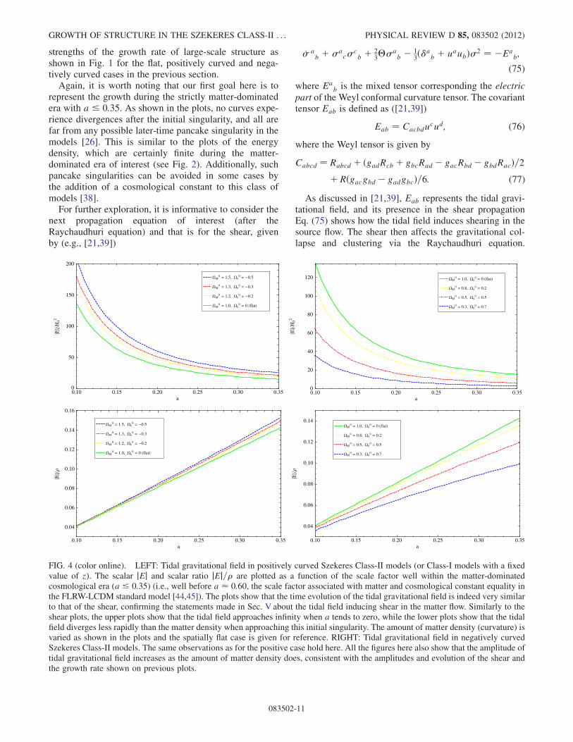
FIG. 4 (color online). LEFT: Tidal gravitational field in positively curved Szekeres Class-II models (or Class-I models with a fixedvalue of z). The scalar jEj and scalar ratio jEj= are plotted as a function of the scale factor well within the matter-dominatedcosmological era (a 0:35) (i.e., well before a 0:60, the scale factor associated with matter and cosmological constant equality inthe FLRW-LCDM standard model [44,45]). The plots show that the time evolution of the tidal gravitational field is indeed very similarto that of the shear, confirming the statements made in Sec. V about the tidal field inducing shear in the matter flow. Similarly to theshear plots, the upper plots show that the tidal field approaches infinity when a tends to zero, while the lower plots show that the tidalfield diverges less rapidly than the matter density when approaching this initial singularity. The amount of matter density (curvature) isvaried as shown in the plots and the spatially flat case is given for reference. RIGHT: Tidal gravitational field in negatively curvedSzekeres Class-II models. The same observations as for the positive case hold here. All the figures here also show that the amplitude oftidal gravitational field increases as the amount of matter density does, consistent with the amplitudes and evolution of the shear andthe growth rate shown on previous plots.

GROWTH OF STRUCTURE IN THE SZEKERES CLASS-II . . . PHYSICAL REVIEW D 85, 083502 (2012)

083502-11

Finally, it is well-known that in the Szekeres models themagnetic part of the Weyl tensor, defined as Hab ¼Cacbdu

cud, vanishes [19,25]. [Here Cacbd is the dual of

Weyl tensor [21,39]].Now, in order to analyze the contribution of the tidal

gravitational field, we plot for the flat and curved SzekeresClass-II models the time evolution of the invariant

E ¼ffiffiffiffiffiffiffiffiffiffiffiffiffiffiffiffiEa

bEba

q: (78)

For that, we first express the invariant in terms of the scalefactor and measurable cosmological parameters as we didfor the shear. We calculate the mixed components Ea

b

using Eq. (75) instead of the definition (76), leading tothe simpler expressions

E11 ¼ E2

2 ¼ 2E33 ¼ 1

3

€H

Hþ 2

3

_H

H

_a

a: (79)

It follows that

E ¼ ffiffiffi2

3

s €H

Hþ 2

_H

H

_a

a

: (80)

Following the same steps as in the previous calculations for, , and , we find

E ¼ ffiffiffi6

p M

a3: (81)

The definition of M allows us to write

M

a3¼ M

2H2: (82)

We can then get E in terms of G, H0, and 0M using Eqs.

(49) and (50). Equation (81) gives finally

jEj ¼ffiffiffi6

p2

0M

a2H2

0G: (83)

Similar to the shear over the expansion ratio, it is useful todefine here the scalar ratio jEj= (see, for example, [26]) inorder to study early time divergences. Using the expression(52) for the energy density we can write this ratio as

jEj

¼ 1ffiffiffi6

p aG

1þ aG: (84)

Our plots for the tidal gravitational field scalar jEj and theratio jEj= are given in Fig. 4 for Class-II (the plots forClass-I with a fixed value of z are exactly the same, and soare the conclusions drawn). The scalar jEj and scalar ratiojEj= are plotted as a function of the scale factor wellwithin the matter-dominated cosmological era. We findthat the time evolution of the tidal field is very similar tothat of the shear and confirms the discussion above aboutthe tidal field inducing shear (according to the shear evo-lution Eq. (75) in the source matter flow. We also see thesame behavior as for the shear at earlier times where thetidal field diverges as a approaches the initial singularity,

but the ratio jEj= does not because the tidal field divergesless rapidly than the matter density as the scale factor goesto zero. The amount of matter density (curvature) is varied,and the figures show how the amplitude of tidal gravita-tional field increases as the amount of matter density does,consistent with what we observed for the shear and thegrowth rate plots.

VI. CONCLUDING REMARKS

We considered the growth rate of large-scale structure inthe Szekeres inhomogeneous cosmological models writtenin the Goode and Wainwright representation. Using theRaychaudhuri equation, we derived exact equations for thegrowth rate for the two Szekeres classes. We explicitlyexpressed the equations in terms of the under/overdensityand measurable cosmological parameters, leading to fur-ther insights on the growth rate of structures in theSzekeres models and also putting them in a frameworkclose to comparison with cosmological observations.In Class-II, the background density is only a function of

time, so we defined the under/overdensity in the standardway, while in Class-I we defined an invariant under/over-density using the quasilocal averaged density over a spatialdomain. For both classes, we found that writing theseequations in terms of these under/overdensities instead ofthe metric functions allows for the growth equations to beremarkably split into two meaningful parts. The first isidentical to the usual growth equations of a perturbedmatter-dominated FLRWmodel. The second part is similarto second-order perturbations, but here the equations de-rived are all exact, and this part represents the nonlinearityof the Szekeres exact solution.We integrated numerically the exact equations obtained

for flat Class-II, curved Class-II, and curved Class-I mod-els. We note that flat Class-I models have no growingmodes and so are of no interest to our purpose here. Forcurved Class-I models, we use a domain delimited by afixed value of z. In all the cases, we found that the Szekeresgrowth rate is up to 3–5 times stronger than that of theperturbed FLRW models. The Szekeres growth (with acorresponding Einstein-de Sitter background) is also foundto be stronger than the well-known nonlinear sphericalcollapse with the difference between the two increasingwith time. This shows that the growth is stronger anddifferent when we use the more general Szekeres inhomo-geneous models where shear and tidal gravitational fieldsare present in the matter source.In order to explore this Szekeres strong growth further,

we derived explicit expressions for the shear scalar andtidal gravitational field part of the Weyl tensor, again all interms of the scale factor and measurable cosmologicalparameters. Our analysis shows and confirms how theshear acts in the Raychaudhuri equation like an effectivesource along with the energy density to enhance gravita-tional collapse and produce stronger growth of structure in

MUSTAPHA ISHAK AND AUSTIN PEEL PHYSICAL REVIEW D 85, 083502 (2012)

083502-12

the Szekeres models. We also derived and plotted the timeevolution of tidal gravitational field, which induces shear-ing in the cosmic fluid flow, as can be seen from the shearevolution equation.

In this analysis, we focused our interest and results to bewell within the matter-dominated cosmological era; Tthatis well after the radiation-dominated era and also wellbefore the equality time between matter dominance andcosmological constant dominance in the FLRW-LCDMstandard model. In other words, here we are only con-cerned with the cosmic era fully dominated by matter.We also plotted the matter energy density during this eraand found that it starts diverging (as expected) close to theinitial singularity, but after that it decreases monotonicallywith no other divergences during this interval, showing thatwe are far away from any possible later-time pancakesingularity in the models. Additionally, such pancake sin-gularities can be avoided by the addition of a cosmologicalconstant to the models as shown in other works. We alsoplotted the time evolution of other scalars, such as the shearover the expansion and the tidal gravitational field over theenergy density and found that they tend to zero whenapproaching the initial singularity, in agreement with pre-vious results that used other considerations.

It is worth noting that the enhancement of the growthfound here in the Szekeres models during the matter-dominated era could suggest a substitute to the argumentthat dark matter is needed when using an FLRW-LCDMmodel during the matter-dominated era in order to explainthe enhanced growth and all the large-scale structure thatwe observe today. Indeed, it is a well-known argument in

FLRW models that dark matter is necessary to enhance thegrowth during the matter-dominated era in order to explainall the presently observed galaxy clusters and superclus-ters. In the Szekeres models the enhanced growth seemspresent with no requirement of dark matter. A similarconclusion was reached in, for example, [54] but fromanalyzing growth in a modified gravity model. Of course,inhomogeneous models with the presence of shear and atidal gravitational field should also be explored to analyzegalaxy rotation curves and other arguments in support ofdark matter. We plan to explore this in follow-up work.Finally, the current results for the growth in Szekeres

expressed within standard schemes of growth rate studiesand in terms of observable cosmological parameters will beuseful toward building a thorough framework where inho-mogeneous Szekeres cosmological models can be com-pared to various current and future cosmological datasets. Comparison of the Szekeres growth rate to currentand future data is beyond the scope of this paper, but it willneed to be done in future and follow-up works.

ACKNOWLEDGMENTS

We thank R. Sussman for valuable comments and M.Troxel for reading the manuscript. M. I. acknowledges thatthis paper is based upon work supported in part by NASAunder Grant No. NNX09AJ55G and by the Department ofEnergy under Grant No. DE-FG02-10ER41310 We alsoacknowledge that the calculations for this work were per-formed on the Cosmology Computer Cluster, which isfunded by the Hoblitzelle Foundation.

[1] H. Stephani, D. Kramer, M. MacCallum, C. Hoenselaers,

and E. Herlt, Exact Solutions of Einstein’s Field Equations

(Cambridge University Press, Cambridge, 2003).[2] A. Krasinski, Inhomogeneous Cosmological Models

(Cambridge University Press, Cambridge, 1997).[3] M-N. Celerier, New Advances in Physics 1, 29

(2007).[4] C. Hellaby and A. Krasinski, Phys. Rev. D 66, 084011

(2002).[5] R. Sussman and J. Triginer, Classical Quantum Gravity

16, 167 (1999).[6] K. Bolejko, Phys. Rev. D 73, 123508 (2006).[7] H. Iguchi, T. Nakamura, and K. I. Nakao, Prog. Theor.

Phys. 108, 809 (2002).[8] H. Alnes, M. Amarzguioui, and O. Gron, Phys. Rev. D 73,

083519 (2006).[9] K. Enqvist and T. Mattsson, J. Cosmol. Astropart. Phys. 02

(2007) 019.[10] D. Garfinkle, Classical Quantum Gravity 23, 4811 (2006).[11] T. Kai, H. Kozaki, K. Nakao, Y. Nambu, and C. Yoo, Prog.

Theor. Phys. 117, 229 (2007).

[12] T. Biswas, R. Mansouri, and A. Notari, J. Cosmol.

Astropart. Phys. 12 (2007) 017.[13] N. Tanimoto and Y. Nambu, Classical Quantum Gravity

24, 3843 (2007).[14] P. Hunt and S. Sarkar, Mon. Not. R. Astron. Soc. 401, 547

(2010).[15] K. Enqvist, Gen. Relativ. Gravit. 40, 451 (2007).[16] M. Ishak, J. Richardson, D. Garred, D. Whittington, A.

Nwankwo, and R. Sussman, Phys. Rev. D 78, 123531(2008).

[17] D. Chung and A. Romano, Phys. Rev. D 74, 103507

(2006).[18] J. Garcia-Bellido and T. Haugboelle, J. Cosmol. Astropart.

Phys. 04 (2008) 003.[19] P. Szekeres, Commun. Math. Phys. 41, 55 (1975).[20] P. Szekeres, Phys. Rev. D 12, 2941 (1975).[21] G. F. R. Ellis and H. van Elst, in Proceedings of the NATO

Advanced Study Institute on Theoretical and

Observational Cosmology, Cargese, France, 1998, edited

by Marc Lachieze-Rey, NATO Science Series C Vol. 541

(Kluwer Academic, Boston, 1999), pp. 1–116.

GROWTH OF STRUCTURE IN THE SZEKERES CLASS-II . . . PHYSICAL REVIEW D 85, 083502 (2012)

083502-13

[22] D. Szafron, J. Math. Phys. (N.Y.) 18, 1673 (1977).[23] W. Bonnor and N. Tomimura, Mon. Not. R. Astron. Soc.

175, 85 (1976).[24] W. Bonnor, A. H. Sulaiman, and N. Tomimura, Gen.

Relativ. Gravit. 8, 549 (1977).[25] S. Goode and J. Wainwright, Mon. Not. R. Astron. Soc.

198, 83 (1982).[26] S. Goode and J. Wainwright, Phys. Rev. D 26, 3315

(1982).[27] W. Bonnor, Classical Quantum Gravity 3, 495

(1986).[28] J. Barrow and J. Stein-Schabes, Phys. Lett. A 103, 315

(1984).[29] J. D. Barrow and J. Silk, Astrophys. J. 250, 432

(1981).[30] A. Krasinski and C. Hellaby, Phys. Rev. D 65, 023501

(2001).[31] C. Hellaby and A. Krasinski, Phys. Rev. D 73, 023518

(2006).[32] K. Bolejko, Phys. Rev. D 75, 043508 (2007).[33] A. Krasinski, Phys. Rev. D 78, 064038 (2008).[34] K. Bolejko and M-N. Celerier, Phys. Rev. D 82, 103510

(2010).[35] B. Nolan and U. Debnath, Phys. Rev. D 76, 104046

(2007).[36] A. Nwankwo, M. Ishak, and J. Thompson, J. Cosmol.

Astropart. Phys.05 (2011) 028.[37] J. Plebanski and A. Krasinski, An Introduction to General

Relativity and Cosmology (Cambridge University Press,Cambridge, 2006).

[38] N. Meures and M. Bruni, Phys. Rev. D 83, 123519(2011).

[39] G. F. R. Ellis, in General Relativity and Cosmology,Proceedings of the International School of Physics

‘‘Enrico Fermi,’’ Course XLVII, edited by R.K. Sachs(Academic Press, New York, 1971).

[40] A. K. Raychaudhuri, Phys. Rev. 98, 1123 (1955).[41] J. Peebles, Large Scale Structure In the Universe

(Princeton University Press, Princeton, 1980).[42] E. Gaztanaga and J. Lobo, Astrophys. J. 548, 47 (2001).[43] W.H. Press, S. A. Teukolsky, W. T. Vetterling, and B. P

Flannery, Numerical Recipes in C (Cambridge UniversityPress, Cambridge, 1992).

[44] M. Ishak, Found. Phys. 37, 1470 (2007).[45] S.M. Carroll, Living Rev. Relativity 4, 1 (2001).[46] R. Sussman, Phys. Rev. D 79, 025009 (2009).[47] R. Sussman, AIP Conference Proc. 1241, 1146 (2010).[48] R. Sussman, Classical Quantum Gravity 28, 235002

(2011).[49] R. Sussman and K. Bolejko, arXiv:1109.1178.[50] In Refs. [46–49] the that we defined here was noted as

ðÞ. Also, as discussed in [48] the sign of ðÞ and theidentification of under-overdensity in inhomogeneous cos-mological models invoke some subtleties. These and otherpoints should be explored within Szekeres models infuture work.

[51] C.W. Misner and D.H. Sharp, Phys. Rev. 136B, B571(1964); M.A. Podurets, Sov. Astron. A. J. 8, 19 (1964);see also, P. S. Wesson and J. Ponce De Leon, Astron.Astrophys. 206, 7 (1988); E. Poisson and W. Israel,Phys. Rev. D 41, 1796 (1990); S. A. Hayward, Phys.Rev. D 49, 831 (1994).

[52] T. Biswas, A. Notari, and W. Valkenburg, J. Cosmol.Astropart. Phys. 11 (2010) 030.

[53] M. Quartin and L. Amendola, Phys. Rev. D 81, 043522(2010).

[54] S. Dodelson and M. Liguori, Phys. Rev. Lett. 97, 231301(2006).

MUSTAPHA ISHAK AND AUSTIN PEEL PHYSICAL REVIEW D 85, 083502 (2012)

083502-14