64
Growth Slowdowns and the Middle-Income Trap Shekhar Aiyar, Romain Duval, Damien Puy, Yiqun Wu, and Longmei Zhang WP/13/71
| Date post: | 04-Jan-2017 |
| Category: |
Documents |
| Upload: | truongtram |
| View: | 221 times |
| Download: | 3 times |

Growth Slowdowns and the Middle-Income Trap
Shekhar Aiyar, Romain Duval, Damien Puy, Yiqun Wu, and Longmei Zhang
WP/13/71
© 2013 International Monetary Fund WP/13/71
IMF Working Paper
Asia and Pacific Department
Growth Slowdowns and the Middle-Income Trap
Prepared by Shekhar Aiyar, Romain Duval, Damien Puy, Yiqun Wu, and Longmei Zhang1
Authorized for distribution by Romain Duval
March 2013
Abstract
The “middle-income trap” is the phenomenon of hitherto rapidly growing economies stagnating at middle-income levels and failing to graduate into the ranks of high-income countries. In this study we examine the middle-income trap as a special case of growth slowdowns, which are identified as large sudden and sustained deviations from the growth path predicted by a basic conditional convergence framework. We then examine their determinants by means of probit regressions, looking into the role of institutions, demography, infrastructure, the macroeconomic environment, output structure and trade structure. Two variants of Bayesian Model Averaging are used as robustness checks. The results—including some that indeed speak to the special status of middle-income countries—are then used to derive policy implications, with a particular focus on Asian economies.
JEL Classification Numbers: C11, C25, O11, O43, O47.
Keywords: growth, slowdown, middle income trap, Bayesian Model Averaging
Authors’ E-Mail Addresses: [email protected]; [email protected]; [email protected]; [email protected]; [email protected]
1 We thank Abdul Abiad, Andy Berg, and participants at the fall 2012 internal IMF seminar, Singapore Management University seminar and KIEP-IMF joint conference for their comments, as well as Lesa Yee for excellent assistance.
This Working Paper should not be reported as representing the views of the IMF. The views expressed in this Working Paper are those of the author(s) and do not necessarily represent those of the IMF or IMF policy. Working Papers describe research in progress by the author(s) and are published to elicit comments and to further debate.
2
Contents Page
I. Setting the Stage ........................................................................................................................... 3
II. Some Stylized Facts .................................................................................................................... 4
III. Identifying Growth Slowdowns ................................................................................................. 8
IV. The Determinants of Growth Slowdowns: Methodology ........................................................ 13
V. The Determinants of Growth Slowdowns: Empirical Results .................................................. 15 A. Institutions .......................................................................................................................... 16 B. Demography........................................................................................................................ 18 C. Infrastructure ....................................................................................................................... 19 D. Macroeconomic Environment and Policies ........................................................................ 20 E. Economic Structure ............................................................................................................. 24 F. Other .................................................................................................................................... 27 G. Summary ............................................................................................................................. 28 H. Are Middle-Income Countries Different? .......................................................................... 30
VI. Policy Implications .................................................................................................................. 32
References ...................................................................................................................................... 55 Figures 1. Cross-Country Comparison ......................................................................................................... 5 2. Growth Trajectories ..................................................................................................................... 6 3. Low-Income Countries ................................................................................................................ 6 4. Slowdown in Latin America: 1970s vs. 1980 .............................................................................. 7 5. Growth Success in Asia ............................................................................................................... 8 6. Is There a Middle Income Trap? ............................................................................................... 12 7. Asian MIC’s Current Strengths and Weaknesses ...................................................................... 36 8. Asian MIC’s Current Strengths and Weaknesses Relative to Other Emerging Regions ........... 37 Tables 1. Distribution of Slowdown Episodes by Region ......................................................................... 11 2. Distribution of Slowdown Episodes by Time Period ................................................................ 11 3. Institutions ................................................................................................................................. 17 4. Demography .............................................................................................................................. 19 5. Infrastructure .............................................................................................................................. 20 6. Macroeconomic Environment and Policies ............................................................................... 23 7. Output Composition ................................................................................................................... 24 8. Trade .......................................................................................................................................... 27 9. Other .......................................................................................................................................... 28 10. Summary Table ........................................................................................................................ 29 11. Middle-Income Countries vs. Full Sample .............................................................................. 31 12. A “Growth Slowdown Risk” Map for Asian Middle-Income Countries ................................. 33 13. A “Trap Map” for Middle-Income Countries .......................................................................... 34 Appendices 1. Bayesian Model Averaging Technique ..................................................................................... 38 2. Tables and Charts ...................................................................................................................... 45

3
I. SETTING THE STAGE
Until recently, the empirical growth literature has implicitly assumed growth to be a smooth process, consistent with a wide variety of theoretical models. One strand of the literature, following the lead of Barro and Sala-i-Martin (1991) and Mankiw, Romer and Weil (1992), has examined the determinants of average GDP per capita growth over a long period (typically a decade or more). Another strand, pioneered by Islam (1995) and Caselli, Esquivel and Lefort (1996) has used dynamic panels rather than cross-country data. In either case, though, what is being estimated is a gradual convergence path, with a single coefficient describing the dynamic behavior of a group of countries.2
But, as is well known, growth dynamics in the real world are more complex than fluctuations around a stable trend. Pritchett (1998) called for more attention to “the hills, plateaus, mountains and plains” evident in the growth record and more recently a literature has arisen that attempts to chart this territory. Growth slowdowns— prolonged periods of stagnation or recession—representing a substantial deviation from the previous norm for a country, have received increasing interest. Clearly, evidence on the factors that determine whether an economy will be subject to such a slowdown is of interest to policy makers. And in practice, anxiety about growth slowdowns has been particularly acute in middle-income countries.
The “middle-income trap” is the phenomenon of hitherto rapidly growing economies stagnating at middle-income levels and failing to graduate into the ranks of high-income countries. Most notably, several Latin American economies, at least until recently, would seem to belong in this category, having failed to achieve high-income levels despite attaining middle-income status several decades ago. By contrast, several East Asian economies have in recent decades provided a template for “success:” continuing to grow rapidly after attaining middle-income status, and thereby attaining per capita income levels comparable to advanced countries.
This paper aims to advance understanding of growth slowdowns and the middle-income trap. It contributes to the literature in several ways. First, it proposes a novel identification procedure for growth slowdowns, one which takes theory seriously rather than simply relying on structural breaks in the time series patterns of economic growth. Second, having identified slowdowns, it shows that these episodes are indeed disproportionately likely to occur in middle-income countries, thereby providing empirical justification for policy concerns about the middle-income trap. Finally, it identifies the determinants of growth slowdowns in a systematic way. Acknowledging the wide uncertainty surrounding the determinants of growth—and, by implication, of growth slowdowns—it relies on a comprehensive set of
2 Following the work of Im, Pesaran, and Shin (2003), some studies have allowed the convergence co-efficient to diverge across countries. But again, for each country the idea is that a single co-efficient adequately captures the dynamical process, and that this co-efficient is the object most worthy of study.

4
explanatory variables and seeks to validate standard probit results using two variations of Bayesian model selection.
The next section shows some stylized facts for a selected group of Asian and Latin American countries to illustrate how heterogeneous growth paths can be, and why growth slowdowns and stagnation at middle-income levels is of such policy relevance. Section 3 describes and executes our identification procedure for growth slowdowns. Section 4 outlines our methodology for exploring their determinants. Section 5 presents a selection of empirical results, and Section 6 draws some policy conclusions for Asia.
II. SOME STYLIZED FACTS
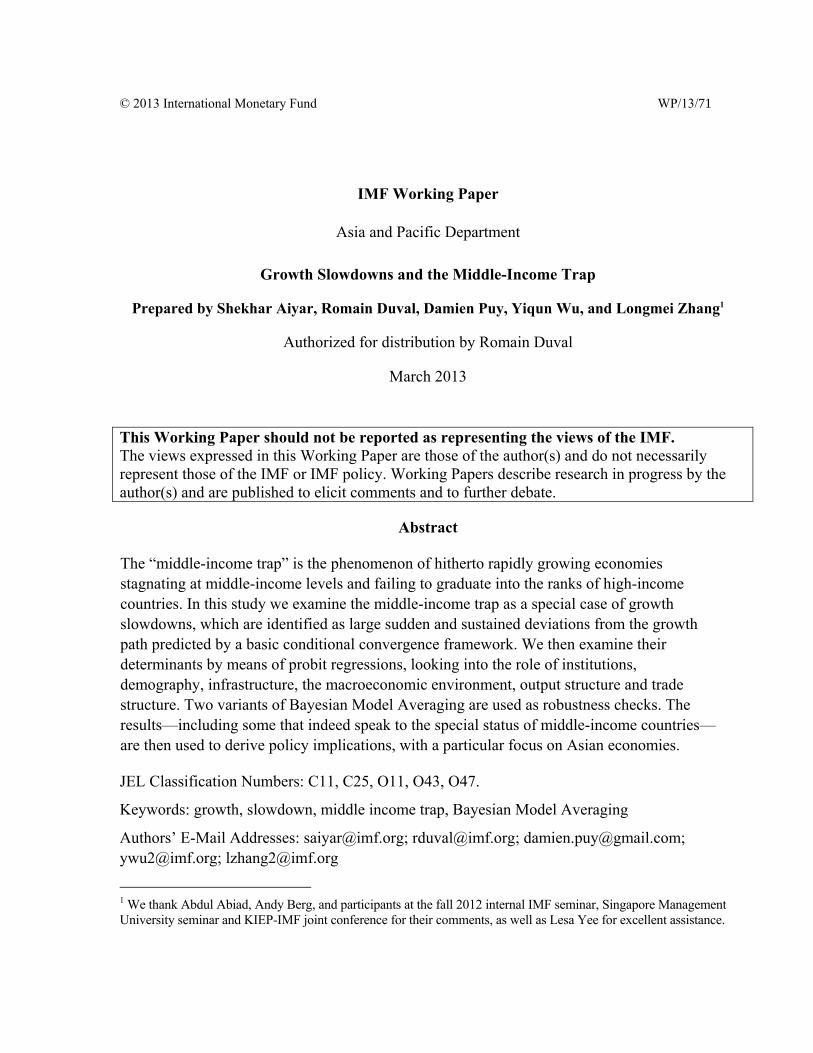
The contrast between several successful East Asian economies and some unsuccessful Latin American economies in the past is illustrated in Figure 1, which shows the evolution of GDP per capita relative to U.S. levels for a set of countries once they have reached an income level of US$ 3000.3 Latin American countries such as Mexico, Peru, and Brazil reached that level before any of the other countries in the chart, hence the longer time series for those countries and the higher intercepts (since U.S. per capita income, the denominator, is smaller the further back in time we go). Despite their relatively late start, two of the Asian “Tigers,” Korea and Taiwan Province of China, have progressed rapidly, increasing their per capita income from 10‒20 percent of U.S. levels to 60–70 percent of U.S. levels.4 In stark contrast to this rapid income convergence, the Latin American countries have stagnated (Brazil and Mexico) or even fallen behind (Peru) in relative terms.
The recent performance of a set of middle-income countries in Asia lies somewhere between the extremes of East Asia and Latin America. China’s trajectory has so far outstripped even that of the earlier East Asian success stories, although it has enjoyed less than a decade above the threshold income level. Malaysia has clearly been more successful than the Latin American comparators, both in absolute and relative terms. Thailand’s trajectory is comparable to the initial growth path of countries like Brazil and Mexico, while Indonesia has performed poorly even relative to Latin America. Since the performance of current middle-income countries in Asia is poised somewhere between the trajectories of East Asia and Latin America, the policy challenge is to ensure that going forward the former trajectory is emulated, not the latter.
3 GDP in constant 2005 international dollars is obtained from the Penn World Tables 7.1. In this section US$3000 is chosen as an illustrative threshold for middle-income countries; the next section will develop the definition of a middle-income country more carefully.
4 Hong Kong SAR and Singapore (and among Latin American countries, Argentina) are not shown in these charts because they had already exceeded the threshold level of US$3000 per capita in 1960, when our time series begins.
5
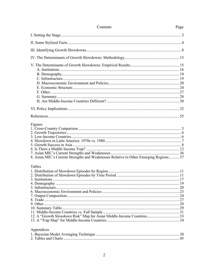
There seems to be a connection between experiencing a growth slowdown and falling into a middle-income trap. Figure 2 shows the same data in log income terms, so that the slopes of the lines can be read as growth rates. It appears that the Latin American countries generally grew at a fairly brisk pace for two or more decades after attaining middle-income status (although still under the growth rates achieved in East Asia). But there is a noticeable slowdown after that, with correspondingly rapid divergence from the East Asian trajectory.
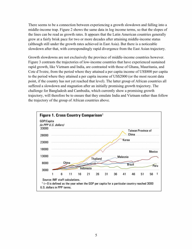
Growth slowdowns are not exclusively the province of middle-income countries however. Figure 3 contrasts the trajectories of low-income countries that have experienced sustained rapid growth, like Vietnam and India, are contrasted with those of Ghana, Mauritania, and Cote d’Ivoire, from the period where they attained a per capita income of US$800 per capita to the period where they attained a per capita income of US$2000 (or the most recent data point, if the country has not yet reached that level). The latter group of African countries all suffered a slowdown and stagnation after an initially promising growth trajectory. The challenge for Bangladesh and Cambodia, which currently show a promising growth trajectory, will therefore be to ensure that they emulate India and Vietnam rather than follow the trajectory of the group of African countries above.
3000
8000
13000
18000
23000
28000
33000
1 6 11 16 21 26 31 36 41 46 51 56
Korea
Taiwan Province of China
China
Indonesia
Mexico
Peru
Source: IMF staff calculations.1 t=0 is defined as the year when the GDP per capita for a particular country reached 3000
U.S. dollars in PPP terms.
Malaysia
Brazil
Thailand
GDP/Capita(in PPP U.S. dollars)
t
Figure 1. Cross Country Comparison1
6
In order to look in greater depth into the drivers of growth slowdowns, Figures 4 through 6 decompose GDP growth rates (in constant international dollars) into factor accumulation and TFP growth, for different regional groupings. The procedure is standard: contributions to GDP growth are calculated for physical capital, human capital, and an expansion of the working age population, and the residual is called TFP growth. Physical capital stocks are calculated on the basis of the perpetual inventory method from the Penn World Tables. Human capital is calculated as a weighted average of years of primary schooling, years of
7.5
8.0
8.5
9.0
9.5
10.0
10.5
1 6 11 16 21 26 31 36 41 46 51 56
KoreaTaiwan Province of China
China
Indonesia
Mexico
Peru
Source: IMF staff calculations.1The GDP per capita is in constant 2005$ PPP adjusted and t= years on X axis. t=0 is defined
as the year when the log(GDP/capita) for a particular country reached US$ 3000 in PPP terms.
Malaysia
Brazil
Thailand
log (GDP/Capita)
t
Figure 2. Growth Trajectories1
6.0
6.5
7.0
7.5
8.0
1 6 11 16 21 26 31 36 41 46 51 56
Vietnam
Cambodia
Source: IMF staff calculations. 1 t=0 is defined as the year when GDP per capita for a particular country reached US$ 800 in PPP terms or the ealiest
data avaliable if the starting value is already higher than 800.The end period for Vietnam and India is when the GDP/capital reached US$ 2000 in PPP terms.
India
log (GDP/Capita)
t
Figure 3. Low-Income Countries1
Bangladesh
Ghana Mauritania
Cote d'Ivoire

7
secondary schooling and years of higher schooling from the Barro-Lee dataset, with the weights comprising Mincerian coefficients obtained by Psacharopuolos (1994).5 As is standard in the literature, a capital share of one-third is assumed (see Gollin, 2002; and Aiyar and Dalgaard, 2009 for justification).
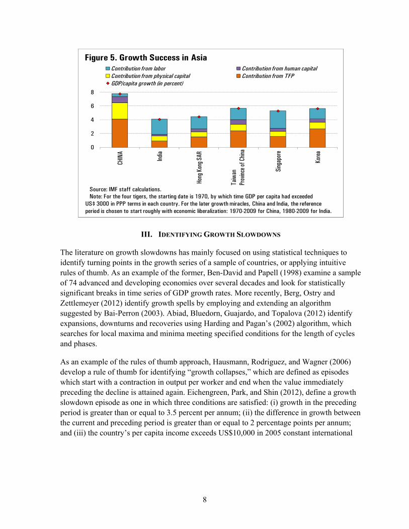
Steep falls in TFP growth appear to have played an important role in past growth slowdowns. This was the case in a number of Latin American countries in the 1980s, with lower growth in physical capital stocks also contributing (Figure 4). In contrast, the success stories of East Asia (and, much more recently and thus far, China and India) are underpinned by robust TFP growth, especially in China and Taiwan Province of China, where they accounted for more than half of all GDP per capita growth (Figure 5).
5 The original idea that this is the appropriate way to introduce human capital into an aggregate production function comes from Bils and Klenow (2000). Here we follow the lead of several papers (Hall and Jones (1999); Aiyar and Dalgaard (2005); Duval and Maisonneuve (2010)) in assuming a piecewise linear formulation for the log of human capital per capita. In particular, the production function is , where H represents the aggregate stock of human capital in the economy, and can be thought of as the economy’s stock of labor times human capital per capita. That is, H = hL, where log h = .134 * pyr + .101 * syr + .068 * hyr. The coefficients in this equation are taken from Psacharopoulos (1994).
-6
-4
-2
0
2
4
6
8
1970‒8
0
1980‒9
0
1970‒8
0
1980‒9
0
1970‒8
0
1980‒9
0
1970‒8
0
1980‒9
0
Contribution from labor Contribution from human capital
Contributions from physical capital Contributions from TFP
GDP/capita growth (in percent)
Figure 4. Slowdown in Latin America: 1970s vs 1980s
Brazil Argentina Peru Mexico
Source: IMF staff calculations.
8
III. IDENTIFYING GROWTH SLOWDOWNS
The literature on growth slowdowns has mainly focused on using statistical techniques to identify turning points in the growth series of a sample of countries, or applying intuitive rules of thumb. As an example of the former, Ben-David and Papell (1998) examine a sample of 74 advanced and developing economies over several decades and look for statistically significant breaks in time series of GDP growth rates. More recently, Berg, Ostry and Zettlemeyer (2012) identify growth spells by employing and extending an algorithm suggested by Bai-Perron (2003). Abiad, Bluedorn, Guajardo, and Topalova (2012) identify expansions, downturns and recoveries using Harding and Pagan’s (2002) algorithm, which searches for local maxima and minima meeting specified conditions for the length of cycles and phases.
As an example of the rules of thumb approach, Hausmann, Rodriguez, and Wagner (2006) develop a rule of thumb for identifying “growth collapses,” which are defined as episodes which start with a contraction in output per worker and end when the value immediately preceding the decline is attained again. Eichengreen, Park, and Shin (2012), define a growth slowdown episode as one in which three conditions are satisfied: (i) growth in the preceding period is greater than or equal to 3.5 percent per annum; (ii) the difference in growth between the current and preceding period is greater than or equal to 2 percentage points per annum; and (iii) the country’s per capita income exceeds US$10,000 in 2005 constant international
0
2
4
6
8
CHIN
A
India
Hong
Kon
g SAR
Sing
apor
e
Kore
a
Contribution from labor Contribution from human capitalContribution from physical capital Contribution from TFPGDP/capita growth (in percent)
Figure 5. Growth Success in Asia
Source: IMF staff calculations.Note: For the four tigers, the starting date is 1970, by which time GDP per capita had exceeded
US$ 3000 in PPP terms in each country. For the later growth miracles, China and India, the reference period is chosen to start roughly with economic liberalization: 1970-2009 for China, 1980-2009 for India.
Taiw
anPr
ovinc
e of C
hina

9
prices.6 This work, in turn, is symmetrically based on Hausmann, Pritchett, and Rodrik’s (2005) analysis of growth accelerations.
This study adopts an alternative approach, one that is better grounded in growth theory. The standard Solow model with identical rates of savings, population growth, depreciation and technological change across countries predicts that poor countries will grow faster than rich countries. Conditional convergence frameworks emphasize that these parameters, and other variables that might influence the steady state, are likely to differ across economies, thus implying that different economies converge to different steady states. Nonetheless, conditional on these country-specific factors, economies further away from the world technology frontier should grow faster than economies close to the frontier. Our approach is to operationalize these strong predictions from theory, and identify slowdowns in terms of large sudden and sustained deviations from the predicted growth path.
We use annual data on per capita income in constant 2005 international dollars to compute a five year panel of GDP per capita growth rates.7 The sample covers 138 countries over 11 periods (1955–2009). Our specification is parsimonious: per capita GDP growth is regressed on the lagged income level and standard measures of physical and human capital.8 For any country at any given point in time, the estimated relationship yields a predicted rate of growth, conditional on its level of income and factor endowments.
Define residuals as actual rates of growth minus estimated rates of growth. A positive residual means that the country is growing faster than expected, while a negative residual means the reverse. Then country i is identified as experiencing a growth slowdown in period t if the two following conditions hold:
0.20 (1)
0.20 (2)
Here p (0.20) denotes the 20th percentile of the empirical distribution of differences in residuals from one time period to another. Intuitively, condition (1) says that between period
6 This work is extended in Eichengreen, Park and Shin (2013), which uses the same methodology for identifying growth slowdowns.
7 We use five-year rolling geometric averages.
8 This represents the most parsimonious established framework for conditional convergence using panel data. It also allows a sharper focus on TFP; what we describe as growth slowdowns in this paper may alternatively be characterized as TFP slowdowns. The rate of investment in physical capital is taken from the Penn World Tables. The rate of investment in human capital across countries is unavailable, so we follow the standard practice of using the stock of human capital instead (e.g., Islam, 1995; Caselli, Esquivel, and Lefort, 1996), calculated using the methodology described in the previous section. Full results are available from the authors on request.

10
t-1 and t the country’s residual became much smaller, that is, its performance relative to the expected pattern deteriorated substantially. To be precise, the deterioration was sufficiently pronounced to place the country-period observation in the bottom quintile of changes in the residual between successive time periods. The second condition is meant to rule out episodes where growth slows down in the current period only to recover in the next, by examining the difference in residuals between periods t-1 and t+1, that is, over a ten year period.9 We are interested here in countries which experience a sustained slowdown.
This methodology has at least three desirable characteristics. First, it makes precise the relative nature of growth slowdowns. At different points in time, the neo-classical growth framework predicts different growth rates for different countries conditional on world technology, current income and factor endowments. By identifying growth slowdowns relative to these factors, and also relative to other economies, the methodology takes theory seriously. Second, and relatedly, it clarifies what needs to be explained. A slowdown in the headline rate of growth could occur, for example, because the country has already attained a high level of income, or because of a temporary shock. But neither of these phenomena stand in need of explanation. Our proposed methodology demarcates those countries which are growing slowly after accounting for expected income convergence and after accounting for short-lived shocks. Finally, the methodology appears to pass the “smell test.” In particular, it captures the episodes that motivated this study, that is, substantial growth slowdown episodes in Latin America in the 1980’s and some slowdowns in Asian countries in the late 1990’s.
Table A.2.1 (in Appendix II) lists all country-periods identified as slowdowns by our methodology. To provide a point of reference, Table A.2.2 also includes a variant of our specification in which the initial panel regression excludes factors of production as regressors, retaining only the initial level of income (absolute convergence), as well as a comparison with slowdown episodes identified by the Eichengreen, Park, and Shin (EPS, 2012) study. Notably, the slowdown episodes identified via the conditional and absolute convergence frameworks are rather similar (the correlation coefficient is 0.97), suggesting that when it comes to sustained shifts away from the convergence path, growth slowdowns are almost synonymous with TFP slowdowns. However, both the conditional and absolute convergence frameworks differ markedly from EPS. The latter study, for example, does not capture the widespread slowdown across Latin America in the 1980s, perhaps because of their narrower focus on countries which already had already attained a per capita income of US$ 10,000 in 2005 international dollars. In fact the majority of countries identified by EPS are developed and oil exporting countries. Our methodology focuses instead on slowdowns at all income levels relative to the predictions of growth theory, allowing us to ask whether slowdowns are empirically more prevalent in middle-income countries (see below).
9 Note that these conditions imply that we cannot identify slowdowns in our sample’s initial period (1955–60), because there is no prior period for comparison, nor in the final period (2005–09), because there is no subsequent period for comparison.
11
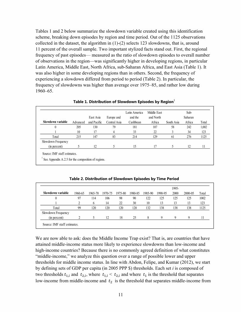
Tables 1 and 2 below summarize the slowdown variable created using this identification scheme, breaking down episodes by region and time period. Out of the 1125 observations collected in the dataset, the algorithm in (1)-(2) selects 123 slowdowns, that is, around 11 percent of the overall sample. Two important stylized facts stand out. First, the regional frequency of past episodes— measured as the ratio of slowdown episodes to overall number of observations in the region—was significantly higher in developing regions, in particular Latin America, Middle East, North Africa, sub-Saharan Africa, and East Asia (Table 1). It was also higher in some developing regions than in others. Second, the frequency of experiencing a slowdown differed from period to period (Table 2). In particular, the frequency of slowdowns was higher than average over 1975–85, and rather low during 1960‒65.
Table 1. Distribution of Slowdown Episodes by Region1
Table 2. Distribution of Slowdown Episodes by Time Period
We are now able to ask: does the Middle Income Trap exist? That is, are countries that have attained middle-income status more likely to experience slowdowns than low-income and high-income countries? Because there is no commonly agreed definition of what constitutes “middle-income,” we analyze this question over a range of possible lower and upper thresholds for middle income status. In line with Abdon, Felipe, and Kumar (2012), we start by defining sets of GDP per capita (in 2005 PPP $) thresholds. Each set i is composed of two thresholds , and , , where , < , and where is the threshold that separates low-income from middle-income and is the threshold that separates middle-income from
Slowdown variable Advanced East Asia and Pacific
Europe and Central Asia
Latin America and the
Caribbean
Middle East and North
Africa South Asia
Sub-Saharan Africa Total
0 205 130 79 181 107 58 242 1,0021 10 17 4 33 22 3 34 123
Total 215 147 83 214 129 61 276 1125Slowdown Frequency
(in percent) 5 12 5 15 17 5 12 11
Source: IMF staff estimates.
1 See Appendix A.2.5 for the composition of regions.
Slowdown variable 1960-65 1965-70 1970-75 1975-80 1980-85 1985-90 1990-95 1995-2000 2000-05 Total
0 97 114 106 98 90 122 125 125 125 10021 2 6 14 22 30 10 13 13 13 123
Total 99 120 120 120 120 132 138 138 138 1125Slowdown Frequency
(in percent) 2 5 12 18 25 8 9 9 9 11
Source: IMF staff estimates.

12
high-income. We assume can take three values, namely 1000, 2000 and 3000 (2005 PPP $) while possible values for range from 12,000 up to 16,000 (in increments of 1000). Using this set of values generates 15 classifications (3 5) spanning a wide range of potential definitions. Figure 6 summarizes the results by plotting, within each income category, the ratio of slowdown episodes to total observations.
The graph makes clear that (i) middle-income countries are, in fact, disproportionately likely to experience growth slowdowns, and (ii) this result is robust to a wide range of income thresholds for defining “middle income.” In our sample, the relative frequency of slowdown episodes for the middle-income category is always significantly higher than for the other two income categories. For the remainder of this paper, when referring to income categories, we will adopt the 2/15 definition, that is, a threshold for low-income economies of 2000 constant (2005 PPP $) dollars and a threshold for high-income economies of 15,000 dollars. The main reason for this choice is that the GDP per capita classification generated by these particular cut-off points is extremely close to the GNI per capita classification employed by the World Bank.10
10 The most recent World Bank classification with data for 2010 is as follows: a country is classified as low-income if its GNI per capita is US$1,005 or less, lower-middle-income if its GNI per capita lies between US$1,006 and US$3,975, upper-middle-income if its GNI per capita lies between US$3,976 and US$12,275, and high income if its GNI per capita is US$12,276 or above. Applying this classification to our sample of 138 countries in 2010 yields 24 low-income countries, 36 lower middle-income countries, 33 upper middle-income countries, and 45 high-income countries. This is very similar to the classification yielded by our 2/15 GDP per capita rule. Actually, there is an overlap of 97 percent between the two methodologies; only eight countries are classified differently.
0.000.020.040.060.080.100.120.140.16
1/12
1/13
1/14
1/15
1/16
2/12
2/13
2/14
2/15
2/16
3/12
3/13
3/14
3/15
3/16
Low income Middle income High incomeSource: IMF staff calculations.11/12 refers to a low income threshold of US$1000 and a high income threshold of US$12000 in PPP terms.2 Frequencies are calculated as the ratio of slowdown episodes to the total number of observations per income class.
Figure 6. Is There a Middle Income Trap?1,2
Income Thresholds*
Freq
uenc
y of S
low
dow
ns
13
IV. THE DETERMINANTS OF GROWTH SLOWDOWNS: METHODOLOGY
Having identified growth slowdowns, we now turn to studying their determinants. The basic strategy is to estimate the impact of various determinants on the probability of a country experiencing a slowdown in a particular period using probit specifications. The main challenge—customary in growth empirics—is that the ex ante set of potential determinants is very large. Like growth itself, growth slowdowns could in principle be generated by a host of factors. Favorable demographics could accelerate growth (reducing the probability of a slowdown), while unfavorable demographics could depress it. Poor institutions—and there are many different types of relevant institutions—could deter innovation, hamper the efficiency of resource allocation, and reduce the returns to entrepreneurship. Structural characteristics of the economy, outward orientation, the state of infrastructure, financial depth, and labor market characteristics could exercise independent effects on growth. And macroeconomic developments, such as terms of trade movements or asset price cycles, could also change the probability of a sustained growth slowdown. Furthermore, there is virtually no theory about why and how middle-income economies may be different. 11
Rather than developing a restrictive theory of growth slowdowns and testing it, this paper follows a strand of recent growth literature in being agnostic about the causes of slowdowns. In what follows we consider as broad a range of factors as possible, culled from a wide reading of the growth literature. The set of regressors comprises 42 explanatory variables grouped into seven categories: (i) Institutions; (ii) Demography; (iii) Infrastructure; (iv) Macroeconomic Environment and Policies; (v) Economic Structure; (vi) Trade structure; and (vii) Other. The actual number of right-hand-side (RHS) variables used is larger still because, as a general rule, we allow the data to speak to whether these variables influence slowdown probabilities in levels or differences. That is, the initial level (at the beginning of the period) and lagged difference of each variable both appear as regressors. Because of the focus on the determinants of sustained slowdowns, one would expect the explanatory variables to matter mostly in differences. However, in some cases the level may pick up important threshold effects, for example some institutional settings may increase the likelihood of a growth slowdown once an economy has reached middle-income status. Table A.2.3 (in Appendix II) provides a summary table of variable units and sources.
The inclusion of a large number of potential regressors, however, has two important drawbacks: model uncertainty and data availability. The first, model uncertainty, is a standard issue in growth empirics where ignorance of the “true” model tends to inflate the number of variables on the RHS or cast doubt on those selected arbitrarily. When the sample size is limited—a rule rather than an exception in growth empirics—classical estimation methods can be of limited use in sorting out robust correlates from irrelevant variables, and growth regressions tend to generate unstable, and sometimes contradictory results (Durlauf,
11 For some recent theoretical attempt at characterizing a middle-income trap, see Agenor and Canuto (2012).

14
Kourtellos, and Tan, 2008). Although the sample size considered in this paper is larger than in many seminal contributions, the issue remains relevant. Our approach to address model uncertainty is to employ Bayesian model averaging techniques. More precisely, after every probit estimation (which is used to generate the main results), two Bayesian model-averaging techniques are applied to the corresponding linear probability model to assess the robustness of the results: the Weighted Average Least Squares (WALS) methodology developed by Magnus, Powell, and Prüfer (2010) and the more standard Bayesian Model Averaging (BMA) developed by Leamer (1978) and popularized by Sala-i-Martin, Doppelhoffer and Miller (2004). Appendix I provides a technical description of the two methods.
The growth literature has seen increasing use of Bayesian averaging techniques, in particular the BMA.12 But WALS is substantially faster than BMA routines. In particular, the computing time increases only linearly with the number of variables using the WALS procedure, while it increases exponentially using BMA. Given the number of regressions and variables considered in this paper, this computational advantage is not negligible. Moreover, WALS relies on a more transparent treatment of ignorance in the form of a Laplace distribution for the parameters and a different scaling parameter for the prior variance.13 Contrasting the two methods allows us to check that our results are robust to changes in the Bayesian averaging method. As regards the growth literature, Magnus, Powell, and Prüfer (2010) have recently shown that some conclusions from Sala-i-Martin, Doppelhoffer, and Miller (2004) were not confirmed by the WALS method, implying that even slight changes to priors and distributions could lead to different diagnosis. As we shall see, it turns out that an overwhelming majority of results are confirmed by both methods. This increases our confidence in the robustness of the conclusions.
The second drawback of considering many potential explanatory variables is that of data availability. Working on 138 countries over 60 years implies inevitable data gaps. In particular, even though the LHS variable consists of 1125 observations with 123 slowdown episodes, data gaps in the RHS variables can restrict drastically the actual sample used for estimation. At one extreme, if one were to use all the 42 explanatory variables in a single estimation at the same time, the actual sample size would drop to less than 170 observations (and 18 slowdowns) due to the poor overlap between the different data categories outlined above. More importantly, using only these 170 observations would imply losing almost all observations before 1995 and observations covering developing countries, thereby restricting the analysis only to recent slowdown episodes that took place in advanced economies. To address at least in part this issue, we group the potential explanatory variables into seven
12 See Moral-Benito (2011) for a survey.
13 The use of a Laplace distribution rather than a normal distribution also leads to finite risk. For a more detailed treatment of the conceptual differences between BMA and WALS, see Magnus, Powell, and Prüfer (2010).

15
categories and estimate their impact on slowdowns separately.14 With relatively large sample sizes within each grouped specification, we can then better discriminate between alternative variables falling into a given category (e.g., institutions). Moreover, for each category of variables, we report not just the probit and Bayesian regression results, but also a set of statistics on sample coverage for the preferred regression by region and time period; this provides some idea of differences in coverage between different categories of variables.15
To summarize, our empirical procedure adopted proceeds through the following steps:
Step 1: For each category, we start by running probit specifications with lagged level and differenced values of all possible explanatory variables within the specific economic category.16 Thus, within the “institutions” category, for a slowdown episode over 1975‒80, the 1975 level of each institutional variable is used together with the change in that variable between 1970 and 1975. This approach minimizes possible endogeneity issues. We use both backward and forward selection procedures to identify a restricted set of robust regressors.17
Step 2: To assess the robustness of the preferred probit specification identified in step 1, Bayesian averaging techniques (BMA and WALS) are used over the full set of variables within the economic category of interest.
Results are presented below for every category and provide (i) the “best” probit specification, that is, the probit including variables selected in Step 1 (ii) the output of Step 2 under the form of individual PIPs (for BMA) and t-ratios (for WALS).
V. THE DETERMINANTS OF GROWTH SLOWDOWNS: EMPIRICAL RESULTS
The empirical growth literature, from which the potential explanatory variables for this study are culled, is too vast to review here. The rationale for the chosen variables is briefly discussed before the presentation of results in each category below, but this is done in an illustrative rather than comprehensive fashion.
14 A similar categorization strategy is followed in Berg, Ostry and Zettlemeyer (2012)
15 Tables in Appendix A.2.4 provide statistics on the sample used for estimation for each category and compare it to the original full sample.
16 The few exceptions to this rule are explained in the text in the next section.
17 The forward selection procedure is to enter the variables one by one, in piecewise fashion, retaining the significant variables. The backward selection procedure starts with the maximal set of variables, drops the least significant variable, and repeats until all remaining variables are significant. We use a 10 percent inclusion (or exclusion) threshold for the forward (backward) procedure. Whenever the set of variables identified as significant differs between the two procedures, we consider the bigger set. In general, there happens to be excellent agreement between the forward and backward procedures in the probit analyses. In the following modules, this agreement should be taken as given unless specified otherwise.
16
A. Institutions
It has been long acknowledged that institutions are important, indeed crucial, for growth, but recently there has been much more attention paid to analyzing the role of different types of institutions. Concurrently, much work has been done in creating cross-country databases with detailed information on institutions.
La Porta, Lopez-de-Silanes, Shleifer, and Vishny (1997, 1998) influentially argued that the quality of a country’s legal institutions—such as legal protection of outside investors—could affect the extent of rent seeking by corporate insiders and thereby promote financial development. This work has engendered several subsequent contributions emphasizing the importance of legal institutions more broadly. Another strand of the literature has emphasized the advantages of limited government (Buchanan and Tullock, 1963; North, 1981 and 1990; and DeLong and Shleifer, 1993). Mauro (1995) finds that corruption lowers investment, thereby retarding economic growth, although Mironov (2005) cautions that this is true of only certain kinds of corruption. Knack and Keefer (1997) provide evidence that formal institutions that promote property rights and contract enforcement help build social capital, which in turn is related to better economic performance. Finally, there is by now a large literature on the relationship between financial openness and growth (e.g., Grilli and Millesi-Feretti, 1995; Quinn, 1997; Edwards, 2001). The lack of a clear consensus in this literature has led Bussiere and Fratscher (2008) to argue that financial liberalization may cause an initial acceleration of growth, but this growth may be difficult to sustain, and may be subject to temporary reversals over a longer horizon.
We use five institutional variables in this module. Four are drawn from the Economic Freedom of the World (EFW) database compiled by the Simon Fraser Institute. The Size of Government index measures the extent of government involvement in the economy, using a range of measures such as general government consumption spending, investment, subsidies and transfers as a percentage of GDP, government ownership of enterprises, and the top marginal income tax rate. The Rule of Law index combines indicators of judicial independence, contract enforcement, military interference in the rule of law, the protection of property rights, and regulatory restrictions on the sale of real property. Freedom to Trade Internationally is constructed from measures of trade taxes, nontariff trade barriers, black market exchange rates and international capital market controls. The Regulation index is an average of selected subindices measuring credit market, labor market and business regulations. All four indices are constructed such that a higher value of the index indicates growth-friendly settings, that is, a higher value indicates better rule of law, smaller government, more freedom to trade and less regulation. The fifth variable used here is the Chinn-Ito index of financial openness (Chinn and Ito, 2006). This is based on binary dummy variables codifying the tabulation of restrictions on cross-border financial transactions reported in the IMF's Annual Report on Exchange Arrangements and Exchange Restrictions (AREAER).
The results are reported in Table 3. The first panel presents coefficient estimates and p-values
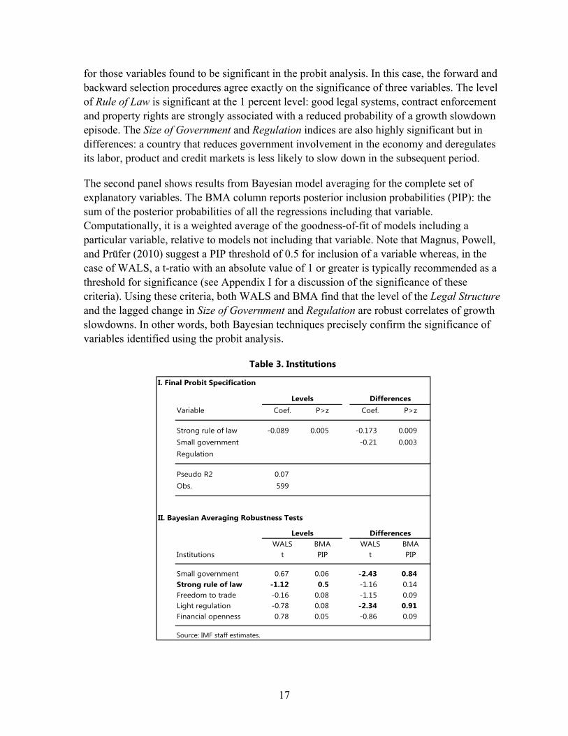
17
for those variables found to be significant in the probit analysis. In this case, the forward and backward selection procedures agree exactly on the significance of three variables. The level of Rule of Law is significant at the 1 percent level: good legal systems, contract enforcement and property rights are strongly associated with a reduced probability of a growth slowdown episode. The Size of Government and Regulation indices are also highly significant but in differences: a country that reduces government involvement in the economy and deregulates its labor, product and credit markets is less likely to slow down in the subsequent period.
The second panel shows results from Bayesian model averaging for the complete set of explanatory variables. The BMA column reports posterior inclusion probabilities (PIP): the sum of the posterior probabilities of all the regressions including that variable. Computationally, it is a weighted average of the goodness-of-fit of models including a particular variable, relative to models not including that variable. Note that Magnus, Powell, and Prüfer (2010) suggest a PIP threshold of 0.5 for inclusion of a variable whereas, in the case of WALS, a t-ratio with an absolute value of 1 or greater is typically recommended as a threshold for significance (see Appendix I for a discussion of the significance of these criteria). Using these criteria, both WALS and BMA find that the level of the Legal Structure and the lagged change in Size of Government and Regulation are robust correlates of growth slowdowns. In other words, both Bayesian techniques precisely confirm the significance of variables identified using the probit analysis.
Table 3. Institutions
I. Final Probit Specification
Variable Coef. P>z Coef. P>z
Strong rule of law -0.089 0.005 -0.173 0.009Small government -0.21 0.003Regulation
Pseudo R2 0.07Obs. 599
II. Bayesian Averaging Robustness Tests
WALS BMA WALS BMAInstitutions t PIP t PIP
Small government 0.67 0.06 -2.43 0.84Strong rule of law -1.12 0.5 -1.16 0.14Freedom to trade -0.16 0.08 -1.15 0.09Light regulation -0.78 0.08 -2.34 0.91Financial openness 0.78 0.05 -0.86 0.09
Source: IMF staff estimates.
Levels Differences
Levels Differences
18
Table A.2.4 panel 1 (in Appendix II) shows the regional coverage of countries in the subsample of data available for the regressions in this category, and compares it to the regional representation in the full sample. Advanced countries are slightly overrepresented in this subsample relative to the full sample, and Eastern Europe and Central Asia slightly underrepresented, but in general the correspondence is quite good. This increases confidence that the results in this module are not being driven by differential sample coverage.
B. Demography
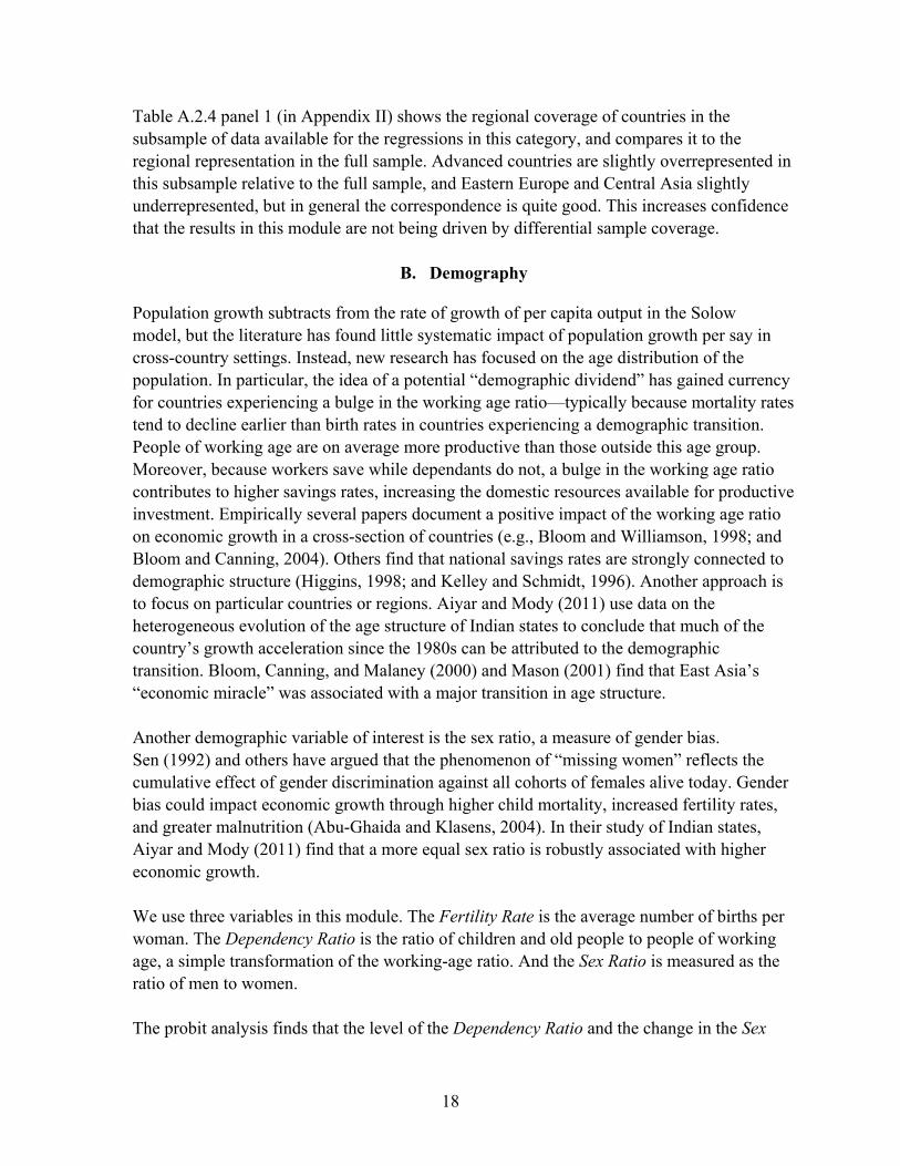
Population growth subtracts from the rate of growth of per capita output in the Solow model, but the literature has found little systematic impact of population growth per say in cross-country settings. Instead, new research has focused on the age distribution of the population. In particular, the idea of a potential “demographic dividend” has gained currency for countries experiencing a bulge in the working age ratio—typically because mortality rates tend to decline earlier than birth rates in countries experiencing a demographic transition. People of working age are on average more productive than those outside this age group. Moreover, because workers save while dependants do not, a bulge in the working age ratio contributes to higher savings rates, increasing the domestic resources available for productive investment. Empirically several papers document a positive impact of the working age ratio on economic growth in a cross-section of countries (e.g., Bloom and Williamson, 1998; and Bloom and Canning, 2004). Others find that national savings rates are strongly connected to demographic structure (Higgins, 1998; and Kelley and Schmidt, 1996). Another approach is to focus on particular countries or regions. Aiyar and Mody (2011) use data on the heterogeneous evolution of the age structure of Indian states to conclude that much of the country’s growth acceleration since the 1980s can be attributed to the demographic transition. Bloom, Canning, and Malaney (2000) and Mason (2001) find that East Asia’s “economic miracle” was associated with a major transition in age structure. Another demographic variable of interest is the sex ratio, a measure of gender bias. Sen (1992) and others have argued that the phenomenon of “missing women” reflects the cumulative effect of gender discrimination against all cohorts of females alive today. Gender bias could impact economic growth through higher child mortality, increased fertility rates, and greater malnutrition (Abu-Ghaida and Klasens, 2004). In their study of Indian states, Aiyar and Mody (2011) find that a more equal sex ratio is robustly associated with higher economic growth. We use three variables in this module. The Fertility Rate is the average number of births per woman. The Dependency Ratio is the ratio of children and old people to people of working age, a simple transformation of the working-age ratio. And the Sex Ratio is measured as the ratio of men to women. The probit analysis finds that the level of the Dependency Ratio and the change in the Sex
19
Ratio are significantly related to slowdown probabilities, with the expected signs (Table 4). That is, a high ratio of dependants to workers, and an increase in the ratio of men to women both increase the probability of a growth slowdown in the subsequent period.18 Both WALS and BMA support this identification.
Table 4. Demography
C. Infrastructure
Infrastructure conveys beneficial externalities to a gamut of productive activities, and in some instances has characteristics of a public good (e.g., a road network might be nonrivalrous at least up to some congestion threshold). For this reason, it has been uncontroversially viewed as positively related to economic growth, at least up to a point. Nonetheless, a survey by Romp and De Hann (2007) shows that the empirical literature has found mixed results, especially when proxies such as public investment are used to measure infrastructure development. More recent contributions, and studies using more direct measures of infrastructure, have generally found a more positive impact of public capital on 18 It should be noted that the initial level of the fertility rate is omitted from the specification, because of its very high correlation with the dependency ratio (0.95). The correlation is substantially lower in differences, allowing both variables to be included in this form.
I. Final Probit Specification
Variable Coef. P>z Coef. P>z
Dependency ration 0.008 0.003Sex ratio 0.075 0.001
Pseudo R2 0.03Obs. 1081
II. Bayesian Averaging Robustness Tests
DemographyWALS BMA WALS BMA
t PIP t PIP
Dependency ratio 2.74 0.7 -1.3 0.05Sex ratio 0.45 0.03 2.29 0.78Fertility rate - - 1.46 0.05
Source: IMF staff estimates.
Levels Differences
Levels Differences
20
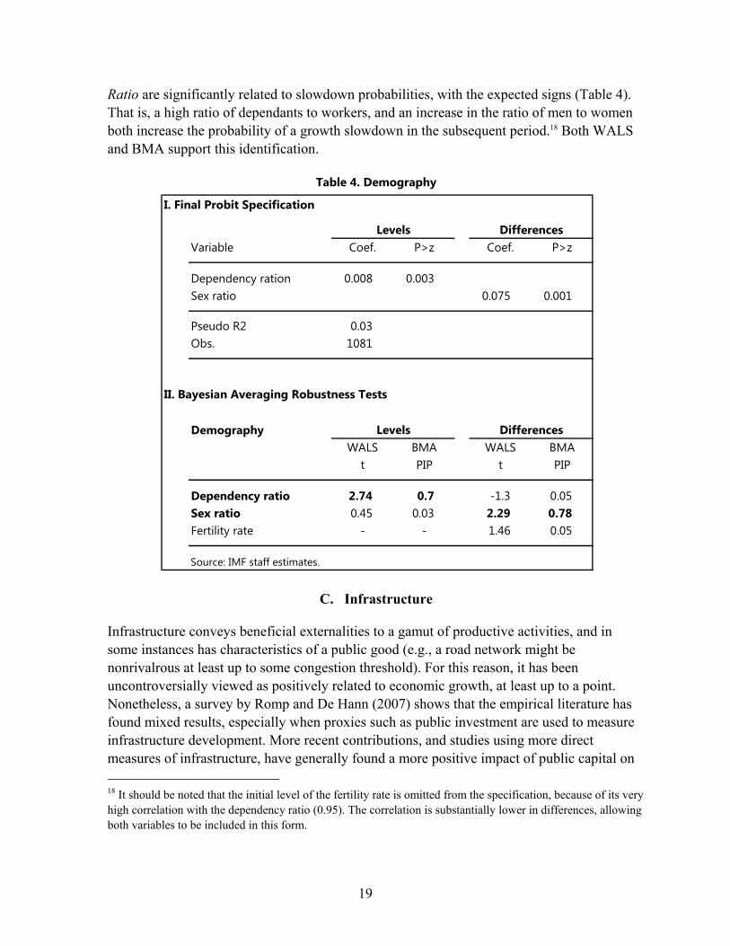
growth (Demetriades and Mamuneas, 2000; Roller and Waverman, 2001; Calderon and Serven, 2004; Erget, Kozluk, and Sutherland, 2009).
We study three kinds of infrastructure development that have been viewed as important by the literature, using data taken from Calderon and Serven (2004). Telephone Lines is the log of telephone lines per 1000 people. Power is the log of gigawatts of generating capacity per 1000 people. And Roads is the log of the length of the country’s road network per square kilometer of land area.
As Table 5 shows, no significant results are found. One interpretation is to note the precise scope of the result here: that poor infrastructure by itself is not responsible for sustained periods of growth slowdowns in the sample (and, conversely, good infrastructure is not sufficient to prevent slowdowns caused by other factors). It is worth noting, however, as we shall see in the next section, that the results are different if we restrict the sample to middle-income countries. So the impact of infrastructure on the probability of slowdowns seems sensitive to the stage of development of an economy.
Table 5. Infrastructure
D. Macroeconomic Environment and Policies
A large variety of macroeconomic factors have been associated with economic growth and shocks to economic growth.
Capital inflows have classically been regarded as conducive to growth, allowing capital to be allocated to wherever its marginal product is highest, besides facilitating consumption smoothing and diversification of idiosyncratic income risk. But the “sudden stops” literature pioneered by Calvo (1998) has emphasized that periods of surging capital inflows are sometimes followed by a cessation or even reversal of the flow, with often severe
I. Final Probit Specification
II. Bayesian Averaging Robustness Tests
InfrastructuresWALS BMA WALS BMA
Levels t PIP t PIP
Telephone lines -0.17 0.06 0.37 0.05Power -0.62 0.07 1.04 0.13Roads -0.72 0.09 -0.72 0.05
Source: IMF staff estimates.
Levels Differences
No infrastructure variable is significant.
21
repercussions. Moreover, certain types of capital flows tend to be flightier and more volatile than others (Ostry and others, 2010). Recent evidence from the global financial crisis suggests high domestic spillovers from reliance on cross-border banking flows (Cetorelli and Goldberg , 2011; Aiyar, 2011, 2012). This is consistent with the “twin crises” literature emphasizing that banking crises and sudden stops are often joined at the hip (Kaminsky and Reinhart, 1999; Glick and Hutchison, 2001). While such shocks may not affect long-term growth, they have been found to lower potential output levels permanently, consistent with a persistent—albeit temporary—impact on potential growth (Cerra and Saxena, 2008).
Similarly, while domestic investment is certainly crucial to economic growth, there is a long tradition in the literature pointing to the perils of over-investment (Schumpeter, 1912; Minsky, 1986, 1992). For example Hori (2007) argues that the investment slump after the Asian crisis of the late 1990s was at least partly due to overinvestment prior to the Investment booms have often been associated with excessive borrowing and rapid accumulation of public and/or external debt. Inflation has also been associated with negative growth outcomes (Fischer, 1993), although Bruno and Easterley (1998) and subsequent contributions emphasize that the relationship is ambiguous when inflation is low to moderate.
There is also a considerable literature on the relationship between growth and price competitiveness. Easterly and others (1993) and Mendoza (1997) find that terms of trade shocks can explain part of the variance in growth across countries. Such shocks could be particularly relevant for countries that are large importers or exporters of fuel and food. Relatedly, there is the concern that exporters specializing in natural resources could be subject to “Dutch Disease.” Prasad, Rajan, and Subramanian (2007) indeed find that exchange rate overvaluation may hinder growth in EMEs as manufacturing is crowded out by less productive sectors.
The names of the variables used in this module are self explanatory. Among those whose definition may not be self evident, Banking Crisis is a dummy variable drawn from the database constructed and updated by Laeven and Valencia (2012), which takes the value of one if the country experienced a banking crisis in any of the five years preceding the current year. Trade Openness is simply a country’s exports plus imports divided by GDP. The four variables Oil Exporters’ Price Shock, Food Exporters’ Price Shock, Oil Importers’ Price Shock, and Food Importers’ Price Shock are included in case the data reveals anything specific about commodity price shocks in countries that are heavily reliant on commodity exports or imports (that is, an effect above and beyond that captured by levels and differences of the country’s Terms of Trade). For instance, Oil Exporter’s Price Shock is defined as the change in the world oil price over the current period times the share of oil exports as percent of GDP. The other three variables are defined analogously, replacing oil by food and exports with imports when relevant.
Looking at Table 6, we find that the initial level of Gross Capital Inflows / GDP is associated with a higher probability of growth slowdown. This result is consistent in principle with

22
either a Dutch Disease type of story or a Sudden Stops story (if the initial high level of inflows were an indicator that inflows are likely to decline over the current period). To discriminate between the two, we examine the correlation between (i) the initial level of capital inflows and the change in the Real Exchange Rate (RER) over the current period; and (ii) the initial level of capital inflows and the change in capital inflows over the current period. The latter correlation is strongly negative while the former is close to zero, supporting the Sudden Stops interpretation. Moreover, a Dutch Disease explanation would sit uneasily with the finding that the level and change in the RER, both of which enter our specification directly, are not found to be significant.
The importance of Sudden Stops is confirmed by the findings in differences: a reduction in Gross Capital Inflows / GDP is associated with a higher probability of a growth slowdown in the subsequent period. Domestic overheating also seems to be strongly associated with slowdowns, thus a rapid increase in an economy’s Investment Share—of the kind witnessed in Asia in the run-up to the crisis on the 1990s—is strongly related to the slowdown probability of the subsequent period. We also find that economies which increase their Trade Openness become less vulnerable to a slowdown in the subsequent period. This may be because trade represents a diversification from purely domestic risks to a mix between domestic and external risks, thereby offering insurance against idiosyncratic domestic shocks.
Finally, an increase in the Public Debt / GDP ratio seems to be associated with a smaller slowdown probability. However, this prima facie counterintuitive relationship appears to be driven by a set of countries whose debts were forgiven as part of the HIPC initiative (and hence registered rapid debt reduction) but which registered poor economic performance. In the final probit specification given in Table 6, the coefficient on public debt ceases to be significant when countries that received HIPC debt relief from the IMF and World Bank in the late 1990s and 2000s are excluded from the sample.19
Furthermore, there is evidence that the probability of a growth slowdown increases non-linearly if the initial level of gross capital inflows is extremely high. This is shown by additional specifications that substitute all variables in levels with a dummy taking the value of 1 if the observation is in the top decile of that variable’s distribution and zero otherwise. The baseline regressions are then run with these seven substitutions of binary variables for continuous variables.20 The gross capital flows dummy turns out to be significant in this exercise.
19 From an accounting perspective HIPIC debt relief instantaneously reduced the public debt ratio by a large amount in recipient countries, despite the fact that nothing “real” might have changed (countries that received such relief were often accruing arrears rather than servicing their debt).
20 Full results are available on request.

23
Table 6. Macroeconomic Environment and Policies
I. Final Probit Specification
Variable Coef. P>z Coef. P>z
Gross capital inflows/GDP 0.028 0.001 -0.016 0.051Investment share 0.059 0.000Trade openness -0.013 0.008Public debt/GDP -0.005 0.040
Pseudo R2 0.1Obs. 462
II. Bayesian Averaging Robustness Tests
WALS BMA WALS BMAInstitutions t PIP t PIP
Inflation -0.79 0.04 0.96 0.05RER 0.33 0.04 0.29 0.04Trade openness 0.48 0.06 -2.09 0.51External debt -0.87 0.04 -0.84 0.04Public debt -0.39 0.05 -2.61 0.92TOT* 0.66 0.05 -1.03 0.10Gross capital inflows / GDP 1.44 0.62 -1.77 0.55Gross capital outflows / GDP 0.02 0.18 -0.65 0.08Investment share 3.50 0.98Price of investment 0.12 0.04Reserves/GDP 0.10 0.05Banking crisis 1.07 0.10Oil_exporters_price_shock* 0.11 0.04Food_exporters_price_shock* 0.00 0.05Oil_importers_price_shock* -0.51 0.06Food_importers_price_shock* 0.00 0.05
* Contemporaneous
Source: IMF staff estimates.
Levels Differences
Levels Differences

24
E. Economic Structure
As an economy develops beyond its pre-capitalist stage, formal employment and output in the manufacturing sector expands, drawing labor from other parts of the economy, especially the initially dominant agricultural sector (Kuznets, 1966). The migration of labor from agriculture to manufacturing, and the corresponding structural transformation of the economy have come to be viewed as the engine of economic development and growth (Harris and Todaro, 1970; Lewis, 1979).
A related aspect of structural transformation is the diversification of output across sectors. Papageorgiou and Spatafora (2012) document an inverse relationship between output diversification (across 12 sectors of the economy) and real income for countries with a GDP per capita below US$5000. Imbs and Wacziarg (2003) argue that there is an inherent link between diversification of the product base and growth as poor countries diversify away from agriculture, although this relationship is nonlinear and may be reversed at higher levels of income.
Based on data from the World Bank’s World Development Indicators, Table 7 presents results from regressing the growth slowdown dummy on the Agriculture Share and the Services Share, with the residual Manufacturing Share omitted. The variables are highly significant in both levels and differences, with a negative sign. That is, a lower initial share of value added in agriculture and services, and a shrinking share of value added in agriculture and services, are associated with a higher probability of a growth slowdown. The results are confirmed by the Bayesian selection procedures.
Table 7. Output Composition
I. Final Probit Specification
Variable Coef. P>z Coef. P>z
Agriculture share -0.012 0.045 -0.039 0.015Services share -0.015 0.035 -0.035 0.011
Pseudo R2 0.04Obs. 606
II. Bayesian Averaging Robustness Tests
Output CompositionWALS BMA WALS BMA
t PIP t PIP
Agriculture share -1.93 0.15 -2.46 0.52Services share -1.9 0.22 -2.47 0.66
Source: IMF staff estimates.
Levels Differences
Levels Differences
25
The most natural way of interpreting these results is that economies undergoing rapid structural change face a concomitant risk of slowdowns. During the process of economic development, surplus labor typically moves from the agricultural and (informal) services sector to formal employment in the newly expanding industrial sector.21 Agriculture and services shrink in relative terms, industry expands, and modern economic growth ensues. But this very process creates risks of a growth slowdown that would not occur in an economy trapped in a low-income equilibrium with no structural transformation and no growth. Needless to say, these results should not be interpreted to argue against structural transformation: clearly growth and the possibility of a slowdown are preferable to stagnation.
Separately, we also examine the relationship between growth slowdowns and economic diversification. We use Papageorgiou and Spatafora’s (2012) index of (lack of) Output Diversification, covering 12 economy-wide sectors from 2000 onwards.22 The reason for considering this index separately is that coverage is poor relative to the other variables in this module. We are only able to examine slowdowns over the period 2000–05, so that the regression collapses to a pure cross-section. Bearing this serious limitation in mind, the results support the thesis that sectoral diversification is associated with a lower probability of growth slowdowns. This could be for two distinct reasons. First, it could simply reflect the relationship between diversification and growth documented by the literature—but we are wary of this explanation in the context of structural transformation, because, as seen above, variables that encourage growth could simultaneously increase the probability of a slowdown episode. Second, and more plausibly, it could reflect that diversification is a form of insurance against idiosyncratic shocks to a particular sector. To the extent that sectoral shocks could lead to slowdown and stagnation in a concentrated economy, diversification reduces the probability of such an event.
Trade Structure
Recent literature has explored several facets of the trade structure of an economy and its relevance to economic growth and resilience. Distance from world and regional economic centers may be conducive to growth through expanded trade opportunities—as well as though better opportunities for foreign investment and knowledge spillovers. Distance can directly raise transport costs and, by segmenting markets, may reduce scale economies for domestic firms. The work of Redding and Venables (2004) showing the association between
21 Classic studies of structural transformation on today’s high-income countries show a pattern whereby initially both industry and services expand at the expense of agriculture. However, many current low-income countries appear to be following a different pattern, especially in Africa. At a very low level of income they have a much higher share of services than advanced countries at a similar stage of development, and this share shrinks initially as the economy undergoes structural transformation (see Bah, 2011).
22 This is a Theil index covering 40 African and 16 Asian economies, with lower values of the index indicating greater output diversification.
26
distance metrics and per capita income has been replicated by other studies using different samples. For example, Boulhol and de Serres (2008) demonstrate that the relationship is valid even within a panel of advanced countries. Further, economies that take advantage of their geographical location by pursuing regional integration might be thought to improve their growth prospects. Ben-David (1993) showed that trade agreements in Europe have enhanced convergence among member countries.
Another strand of the literature looks at export diversification, which has generally been found to be favorably related to growth, especially at an early stage of development. Koren and Tenreyro (2007) show that economic diversification can increase the resilience of low-income countries to external shocks, while Agosin (2003) provides evidence that export diversification has a positive impact on growth in emerging economies. Case studies like Gartner and Papageorgiou (2011) also reach similar conclusions.
Our data on Distance (GDP Weighted) comes from the World Bank. For each country i, it sums the distance to every other country in the world j, weighting each distance by the share of country j in world GDP. Thus, the index will be small for countries close to large, economically important countries (e.g., Canada) and large for countries which are geographically isolated from economic centers (e.g., Pacific Island economies). Therefore the index measures the extent to which a country’s geographic location is unfavorable. Regional Integration is the amount of intra-regional trade (exports plus imports) undertaken by a country relative to its total trade. (Lack of) Export Diversification is a Theil index calculated by Papageorgiou and Spatafora (2012) using product data at the four-digit SITC level.
The probit analysis suggests that Distance and Regional Integration are both important determinants of growth slowdowns, and this is confirmed by the Bayesian model selection. The greater the GDP-weighted distance of a country from potential trade partners, the higher the probability of a slowdown. And the greater the share of intra-regional trade undertaken by a country, the less likely is a slowdown. Export Diversification is not selected as significant, but a closer analysis shows that introducing Export Diversification in tandem with Distance and Regional Integration results in “throwing away” a considerable amount of data on diversification because of limited sample coverage for the other two variables. Worse, the omitted data is disproportionately from African countries, which may stand to benefit the most from diversification if the relationship between diversification and growth is non-linear. When estimating the relationship between growth slowdowns and Export Diversification separately,23 we find that a diversified export base is indeed associated with a lower probability of slowdown for the larger sample.
23 Full results are available upon request.

27
Table 8. Trade
F. Other
In this last module we consider variables that do not fit easily under any of the previous economic categories. ELF is an index of ethno-linguistic fractionalization, which has often been associated with poor social capital and negative growth outcomes (Easterly and Levine, 1997; and La Porta and others, 1999). Tropics measure the fraction of a country’s land area that lies in the tropical zone. Various features of this climatic zone, such as poorer land productivity and conditions more favorable to vector-borne diseases could have an adverse impact on growth (Sachs, 2012; and Masters and McMillan, 2001). Being a Spanish Colony in the past and having a large Buddhist population are variables that Sala-i-Martin, Dopplehofer, and Miller (2004) find to be significantly associated with growth even after controlling for other institutional and cultural factors. Finally, Wars and Civil Conflicts, and Natural Disasters can clearly depress growth.24
The variables in this module are either time-invariant or plausibly exogenous, so they enter the specifications contemporaneously rather than with a lag. Moreover, the nature of the
24 Various measures of income distribution were also considered as dependant variables, but the time series was too short to obtain meaningful results.
I. Final Probit Specification
Variable Coef. P>z Coef. P>z
Distance 0.116 0.007Regional Integration -0.008 0.011
Pseudo R2 0.02Obs. 698
II. Bayesian Averaging Robustness Tests
TradeWALS BMA WALS BMA
t PIP t PIP
Distance 1.77 0.35Regional Integration -1.77 0.34 0.31 0.05Weak Export Diversification 0.47 0.19 0.76 0.05
Source: IMF staff estimates.
Levels Differences
Levels Differences

28
variables considered means they only enter in levels, not in differences. We find that Wars and Civil Conflicts and the fraction of a country’s area in the Tropics are both significantly positively associated with the probability of a growth slowdown.
Table 9. Other
G. Summary
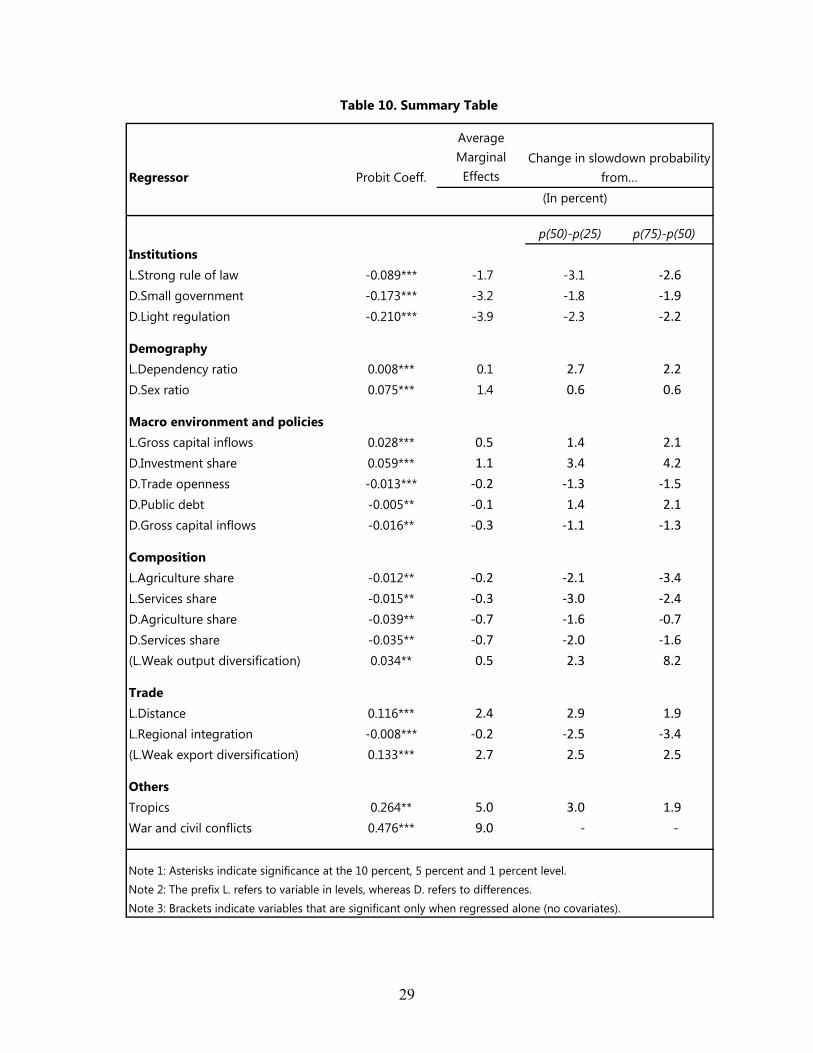
Table 10 below summarizes the results of the empirical analysis. It lists, by module, all the variables found selected as significant. Apart from showing the average marginal effect of each variable, it attempts to give a flavor of the magnitude of their impact on slowdown probabilities, as well as on possible asymmetries in this impact arising from the distributional characteristics of the variable. The last two columns of the table show the impact on the probability of a slowdown if variable X moves from the 25th percentile of the distribution of X to the 75th percentile (integrating over all possible values for other variables in the module). Some of the variables amenable to policy are seen to have a very substantial impact on slowdown probabilities. For example, taken at face value, the results imply that improving trade integration from the 25th percentile level to the median lowers the probability of a slowdown by 2.5 percentage points, while a further move to the 75th percentile lowers that probability by a further 3.4 percentage points.
I. Final Probit Specification
Variable Coef. P>z Coef. P>z
Tropics 0.264 0.026Wars and civil conflicts 0.476 0.003
Pseudo R2 0.02Obs 918
II. Bayesian Averaging Robustness Tests
OthersWALS BMA WALS BMA
t PIP t PIP
ELF -0.62 0.04 - -Buddhist 0.18 0.03 - -Spanish colony 0.31 0.05 - -Tropics 1.7 0.36 - -Natural distasters -0.26 0.03 - -Wars and civil conflicts 2.08 0.59 - -
Source: IMF staff estimates.
Levels Differences
Levels Differences
29
Table 10. Summary Table
Regressor Probit Coeff.
Average Marginal Effects
p(50)-p(25) p(75)-p(50)InstitutionsL.Strong rule of law -0.089*** -1.7 -3.1 -2.6
D.Small government -0.173*** -3.2 -1.8 -1.9
D.Light regulation -0.210*** -3.9 -2.3 -2.2
DemographyL.Dependency ratio 0.008*** 0.1 2.7 2.2
D.Sex ratio 0.075*** 1.4 0.6 0.6
Macro environment and policiesL.Gross capital inflows 0.028*** 0.5 1.4 2.1
D.Investment share 0.059*** 1.1 3.4 4.2
D.Trade openness -0.013*** -0.2 -1.3 -1.5
D.Public debt -0.005** -0.1 1.4 2.1
D.Gross capital inflows -0.016** -0.3 -1.1 -1.3
CompositionL.Agriculture share -0.012** -0.2 -2.1 -3.4
L.Services share -0.015** -0.3 -3.0 -2.4
D.Agriculture share -0.039** -0.7 -1.6 -0.7
D.Services share -0.035** -0.7 -2.0 -1.6
(L.Weak output diversification) 0.034** 0.5 2.3 8.2
TradeL.Distance 0.116*** 2.4 2.9 1.9
L.Regional integration -0.008*** -0.2 -2.5 -3.4
(L.Weak export diversification) 0.133*** 2.7 2.5 2.5
OthersTropics 0.264** 5.0 3.0 1.9
War and civil conflicts 0.476*** 9.0 - -
Note 1: Asterisks indicate significance at the 10 percent, 5 percent and 1 percent level.Note 2: The prefix L. refers to variable in levels, whereas D. refers to differences. Note 3: Brackets indicate variables that are significant only when regressed alone (no covariates).
Change in slowdown probability from…
(In percent)

30
H. Are Middle-Income Countries Different?
Since we have already established that middle-income countries (MICs) differ from others in experiencing a higher frequency of slowdowns, it is natural to ask whether any of the determinants examined above act on MICs differently. To explore this possibility we restrict the sample to MICs and repeat all the regressions described in the previous subsections. Table 11 shows how the results differ across the full sample and the restricted sample. A blank entry in the MIC column indicates implies that the variable is not selected as significant in the restricted sample despite being significant in the full sample. A blank entry in the full sample column implies the reverse.
Two points are worth noting with respect to institutions. First, Government Size replaces the Rule of Law as the most significant institution variable in levels. It may be that at very low levels of income, the development of a basic framework of property rights and contract enforcement has a large impact in staving off slowdowns, but once this condition is more or less satisfied the capacity of the private sector to grow and innovate becomes relatively more important. The capacity of the private sector to expand may be hampered by the extent of government involvement in the economy, which therefore shows up as significant for MICs. Related to this, the coefficient on Regulation in differences is twice as large for MICs than for the full sample of countries, suggesting again that deregulation is a particularly important channel for guarding against slowdowns in MICs. This is consistent with Aghion and others’ (2005) emphasis on distance-to-frontier effects: the marginal impact of regulation is likely to be greater closer to the world technology frontier, where the key to productivity gains lies in innovation rather than absorption of existing technology.
Second, the level of infrastructure development is important in MICs, where insufficient Road Networks and Telephone Lines per head both emerge as potential risk factors for growth. In line with some of the results on institutions, infrastructure development appears to matter more once the low-income stage of development has been passed.
On trade, it should be noted that the result that Regional Integration reduces the probability of a slowdown is obtained for MICs only after dropping outliers. That is, the reported coefficient is for a sample of MICs in which the bottom and top deciles—by degree of regional trade integration—have been excluded. Including these outliers drives the significance of the relationship below conventional limits. This suggests threshold effects: a marginal increase in regional integration has little effect if the country is initially very poorly integrated or very highly integrated.25
25 It is possible that regional integration, especially the way it is measured in this study, is related to product sophistication. For example, if an economy that was initially exporting mainly resource-based commodities begins to integrate into regional vertical supply chains, that would tend to increase both regional integration as well as product sophistication. But data coverage is much better for regional integration than for product
(continued)
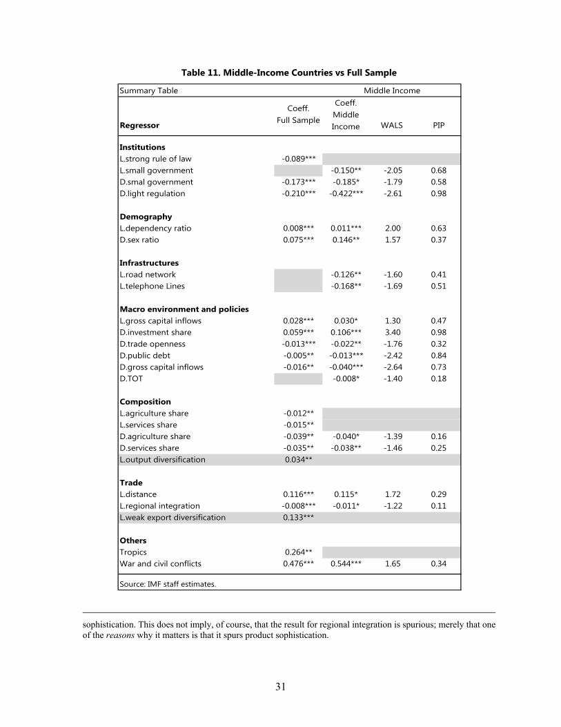
31
Table 11. Middle-Income Countries vs Full Sample
sophistication. This does not imply, of course, that the result for regional integration is spurious; merely that one of the reasons why it matters is that it spurs product sophistication.
Summary Table
Regressor
Coeff. Full Sample
Coeff. Middle Income WALS PIP
InstitutionsL.strong rule of law -0.089***L.small government -0.150** -2.05 0.68D.smal government -0.173*** -0.185* -1.79 0.58D.light regulation -0.210*** -0.422*** -2.61 0.98
DemographyL.dependency ratio 0.008*** 0.011*** 2.00 0.63D.sex ratio 0.075*** 0.146** 1.57 0.37
InfrastructuresL.road network -0.126** -1.60 0.41L.telephone Lines -0.168** -1.69 0.51
Macro environment and policiesL.gross capital inflows 0.028*** 0.030* 1.30 0.47D.investment share 0.059*** 0.106*** 3.40 0.98D.trade openness -0.013*** -0.022** -1.76 0.32D.public debt -0.005** -0.013*** -2.42 0.84D.gross capital inflows -0.016** -0.040*** -2.64 0.73D.TOT -0.008* -1.40 0.18
CompositionL.agriculture share -0.012**L.services share -0.015**D.agriculture share -0.039** -0.040* -1.39 0.16D.services share -0.035** -0.038** -1.46 0.25L.output diversification 0.034**
TradeL.distance 0.116*** 0.115* 1.72 0.29L.regional integration -0.008*** -0.011* -1.22 0.11L.weak export diversification 0.133***
OthersTropics 0.264**War and civil conflicts 0.476*** 0.544*** 1.65 0.34
Source: IMF staff estimates.
Middle Income

32
Finally, the tentative finding that both Output Diversification and Trade Diversification are negatively associated with the probability of a slowdown disappears when the sample is restricted to MICs. This is consistent with the literature emphasizing that diversification is particularly associated with economic growth in low-income countries transitioning out of a primarily agriculture-based economy, and that the relationship might even reverse beyond a certain level of income (Papageorgiou and Spatafora, 2012; Imbs and Wacziarg , 2003).
VI. POLICY IMPLICATIONS
The chief policy implications lie in the variables identified as significant in the previous section. They are hardly controversial, but they do provide intellectual ballast for supportive reforms in areas identified as important, and for a more detailed academic focus and further research in those areas.26 Moreover, some of the identified variables are clearly more amenable to policy than others, especially over short time horizons. Prudential regulation to limit the build-up of excessive capital inflows and cushion the impact of a sudden stop, measures to enhance regional trade integration, public investment in infrastructure projects, and deregulation in areas where red tape is stifling private activity are all examples of reforms that can be enacted by incumbent governments in a relatively short period of time. At the other extreme, a country’s geographical distance from potentially attractive trade partners, and its climatic conditions are essentially immune to policy. In between there are variables that could be influenced by policy but only over the medium- to long-term, such as demographic trends (e.g., through incentives to reduce fertility and combat gender discrimination) and the rule of law.
Table 12 below constructs an illustrative “growth slowdown risk” map for seven Asian MICs in seven categories identified in the previous section. In each category we apply the MIC coefficients listed in Table 11 to the latest available data for the Asian MICs, to calculate the probability of an imminent slowdown over the next five years.27 Then we look at the rankings of the seven Asian MICs under each category, with one signifying the greatest risk of slowdown in that category and seven signifying the least risk. The red color indicates lower (“bad”) rankings while the green color denotes higher (“good”) ones, relative to other economies featured in the table.
26 For example, one issue that this paper has not taken up is whether the impact of distance to frontier on economic growth – and, by extension, on the probability of a slowdown – is itself a function of time. It may be argued that technology is more easily disseminated today, with greater stocks of FDI or widespread internet connectivity, than in earlier periods of time. Another issue that might benefit from further research is the time-varying role of TFP in MICs; it is possible that once these countries have exhausted the “spurt” from the accumulation of factors of production, they must rely increasingly on productivity gains to engender further growth. This is suggested, for example, by Agenor and Canuto (2012)
27 We omit the category “Other” from the previous section, covering variables largely irrelevant from a policy perspective. The category “Infrastructure” is split into two columns, Communications and Road transport, because probit specifications for these variables are run separately due to their strong correlation.

33
Taken at face value, the empirical results imply that, compared with other Asian economies, Malaysia, the Philippines and China would face a larger risk of growth slowdown stemming from institutions. Vietnam, India, and Indonesia are most at risk of a slowdown arising from a lack of transport and communications infrastructure. On trade, India could do more to pursue regional integration, while Thailand and the Philippines are relatively well integrated. It should be stressed that Table 12 does not rank countries according to the levels of the underlying variables, but instead according to the (weighted) mix of levels and differences that came out significant in the empirical analysis. For instance, the higher risk of slowdown arising from institutions in Malaysia than in Vietnam does not mean that the latter has “better” institutions than the latter but rather that its institutions have improved more rapidly over the last period of the sample—since it is the difference that is found to matter for two out of the three statistically significant institutional variables in the regression analysis, see Table 11.
Table 12. A “Growth Slowdown Risk” Map for Asian Middle-Income Countries
Country Institutions Demography Communication Road Output
Composition Macroeconomic
Factors Trade
China
India
Indonesia
Malaysia
Philippines
Thailand
Vietnam
Table 13 expands this methodology to a broader set of MIC comparators from Latin America and MENA. Two noteworthy conclusions can be drawn from this regional comparison. First, the empirical results imply that compared with other regions, Asia stands at higher risk of a growth slowdown arising from infrastructure, in particular communication infrastructure. While the indicators chosen here focus on transport and communications, it is likely that this extends to infrastructure more generally: several countries in the region need to develop new infrastructure and upgrade existing infrastructure in power generation, public transit systems, freight and ports. Second, the region compares rather favorably with others in the trade category. Regional integration and vertical supply chains in Asian MICs compare favorably with Latin American and MENA comparators. Even India and Indonesia, which lag behind the other Asian MICs in this category, are well situated compared to the broader sample. So this is an area of strength, which should serve the region well as a buffer against growth slowdowns.

34
Table 13. A “Trap Map” for Middle-Income Countries
Country Institutions Demography Communication RoadOutput
Composition Macroeconomic
Factors Trade
China
India
Indonesia
Malaysia
Philippines
Thailand
Vietnam
Argentina
Bolivia
Brazil
Chile
Colombia
Costa Rica
Ecuador
El Salvador
Guatemala
Honduras
Mexico
Panama
Paraguay
Peru
Uruguay
Iran
Jordan
Egypt
Algeria
Morocco
Tunisia
Developing Asia
Latam
MENA
Developing Asia
Latam
MENA

35
Finally, Figures 7 and 8 perform similar comparisons, but now focusing only on the levels of the variables—with the exception of the “macroeconomic factors” category for which first differences over 2008-2012 are also considered in line with the empirical results. The purpose here is to identify each country’s current relative strengths and weaknesses, and thereby to determine where it has most room for reducing risks of a sustained growth slowdown at some point in the future. This approach implies some departure from—although it remains qualitatively consistent with—the empirical analysis, since as noted above the latter identifies a mix of levels and differences as drivers of slowdown probabilities. For simplicity and illustrative purposes, in Figures 7 and 8 rankings in each category are computed here as simple averages of the rankings on the variables belonging to this category, and only a subset of those variables is considered. The results are shown in the form of “spider webs:” the larger the area within each country’s “spider web,” the better its current settings in the dimension considered.
The main findings from both figures are fairly consistent with those from Tables 10 and 11. Some Asian economies are less well-positioned than others and have therefore greater room for reducing risks of a growth slowdown further down the road. Also, compared with other MICs, Asian economies have on average most room for improvement on institutions, with some of them also in need of more and better infrastructure. On macroeconomic factors, while Asia’s recent growth has typically benefitted from its comparatively strong capital inflows and increased investment rates, these also come with risks. On other dimensions, Asian MICs often compare favorably to their emerging market counterparts in other regions.
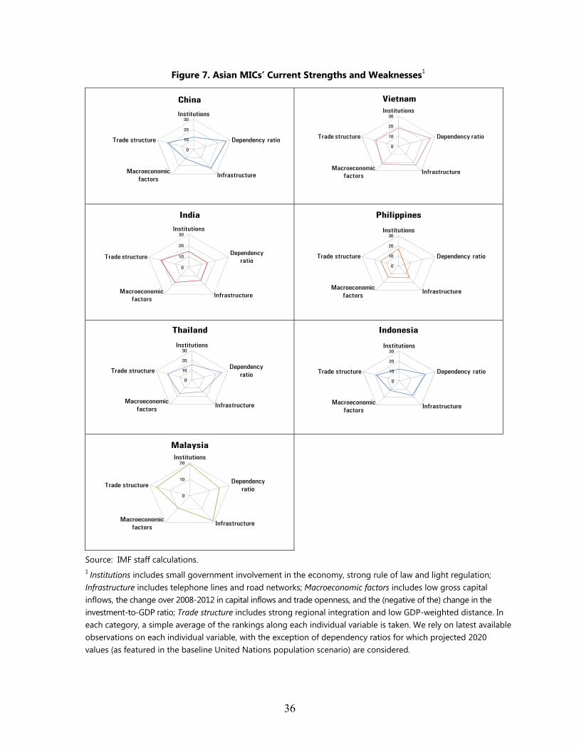
36
Figure 7. Asian MICs’ Current Strengths and Weaknesses1
Source: IMF staff calculations. 1 Institutions includes small government involvement in the economy, strong rule of law and light regulation; Infrastructure includes telephone lines and road networks; Macroeconomic factors includes low gross capital inflows, the change over 2008-2012 in capital inflows and trade openness, and the (negative of the) change in the investment-to-GDP ratio; Trade structure includes strong regional integration and low GDP-weighted distance. In each category, a simple average of the rankings along each individual variable is taken. We rely on latest available observations on each individual variable, with the exception of dependency ratios for which projected 2020 values (as featured in the baseline United Nations population scenario) are considered.
0
10
20
30Institutions
Dependency ratio
InfrastructureMacroeconomic
factors
Trade structure
China
0
10
20
30Institutions
Dependency ratio
InfrastructureMacroeconomic
factors
Trade structure
Vietnam
0
10
20
30Institutions
Dependency ratio
InfrastructureMacroeconomic
factors
Trade structure
India
0
10
20
30Institutions
Dependency ratio
InfrastructureMacroeconomic
factors
Trade structure
Philippines
0
10
20
30Institutions
Dependency ratio
InfrastructureMacroeconomic
factors
Trade structure
Thailand
0
10
20
30Institutions
Dependency ratio
InfrastructureMacroeconomic
factors
Trade structure
Indonesia
0
10
20Institutions
Dependency ratio
InfrastructureMacroeconomic
factors
Trade structure
Malaysia
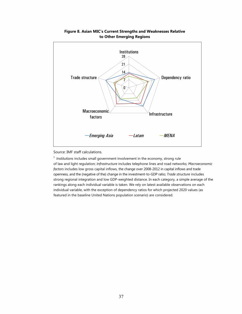
37
Figure 8. Asian MIC’s Current Strengths and Weaknesses Relative to Other Emerging Regions
Source: IMF staff calculations. 1 Institutions includes small government involvement in the economy, strong rule of law and light regulation; Infrastructure includes telephone lines and road networks; Macroeconomic factors includes low gross capital inflows, the change over 2008-2012 in capital inflows and trade openness, and the (negative of the) change in the investment-to-GDP ratio; Trade structure includes strong regional integration and low GDP-weighted distance. In each category, a simple average of the rankings along each individual variable is taken. We rely on latest available observations on each individual variable, with the exception of dependency ratios for which projected 2020 values (as featured in the baseline United Nations population scenario) are considered.
0
7
14
21
28Institutions
Dependency ratio
InfrastructureMacroeconomic
factors
Trade structure
Emerging Asia Latam MENA
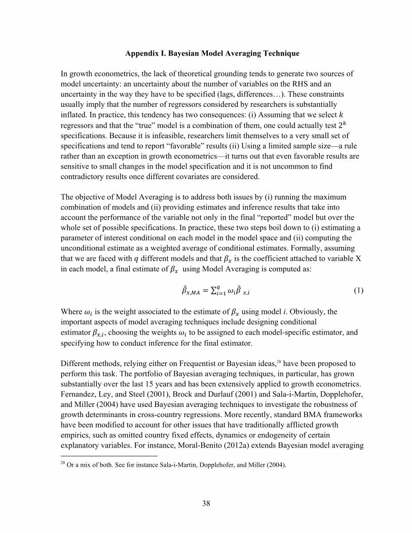
38
Appendix I. Bayesian Model Averaging Technique In growth econometrics, the lack of theoretical grounding tends to generate two sources of model uncertainty: an uncertainty about the number of variables on the RHS and an uncertainty in the way they have to be specified (lags, differences…). These constraints usually imply that the number of regressors considered by researchers is substantially inflated. In practice, this tendency has two consequences: (i) Assuming that we select regressors and that the “true” model is a combination of them, one could actually test 2 specifications. Because it is infeasible, researchers limit themselves to a very small set of specifications and tend to report “favorable” results (ii) Using a limited sample size—a rule rather than an exception in growth econometrics—it turns out that even favorable results are sensitive to small changes in the model specification and it is not uncommon to find contradictory results once different covariates are considered. The objective of Model Averaging is to address both issues by (i) running the maximum combination of models and (ii) providing estimates and inference results that take into account the performance of the variable not only in the final “reported” model but over the whole set of possible specifications. In practice, these two steps boil down to (i) estimating a parameter of interest conditional on each model in the model space and (ii) computing the unconditional estimate as a weighted average of conditional estimates. Formally, assuming that we are faced with different models and that is the coefficient attached to variable X in each model, a final estimate of using Model Averaging is computed as:
, ∑ , (1) Where is the weight associated to the estimate of using model i. Obviously, the important aspects of model averaging techniques include designing conditional estimator , , choosing the weights to be assigned to each model-specific estimator, and specifying how to conduct inference for the final estimator. Different methods, relying either on Frequentist or Bayesian ideas,28 have been proposed to perform this task. The portfolio of Bayesian averaging techniques, in particular, has grown substantially over the last 15 years and has been extensively applied to growth econometrics. Fernandez, Ley, and Steel (2001), Brock and Durlauf (2001) and Sala-i-Martin, Dopplehofer, and Miller (2004) have used Bayesian averaging techniques to investigate the robustness of growth determinants in cross-country regressions. More recently, standard BMA frameworks have been modified to account for other issues that have traditionally afflicted growth empirics, such as omitted country fixed effects, dynamics or endogeneity of certain explanatory variables. For instance, Moral-Benito (2012a) extends Bayesian model averaging 28 Or a mix of both. See for instance Sala-i-Martin, Dopplehofer, and Miller (2004).
39
techniques to panel data models with country-specific fixed effects whereas Tsangarides (2004), Chen, Mirestean and Tsangarides (2009), Durlauf, Kourtellos, and Tan (2008) and Eicher, Lenkoski, and Raftery (2009) address the issue of model uncertainty in the presence of endogeneity.29 In this paper, we rely on the following two Bayesian Frameworks: The “traditional” BMA first applied in growth econometrics by Fernandez, Ley, and Steel
(2001) and recently used in Masanjala and Papageorgiou (2008). The WALS developed by Magnus, Powell, and Prüfer (2010) and also applied to growth
empirics.
Note that because we are working with (i) a panel dataset and (ii) a binary dependent variable, one would ideally use Bayesian Averaging of (dynamic) probit models to investigate the sensitivity of probit coefficients across all specifications. However, research in this area is still ongoing and contributing to this literature is beyond the scope of our paper. More importantly, we emphasize that the scope of averaging methods in our framework is smaller than in other contexts. Key results and interpretations are derived from probit estimations, and Bayesian Averaging algorithms are used only as a robustness check—rather than as an estimation tool. In particular, we are interested in checking that the « strongest » regressors which have been selected by both forward and backward probit procedures are indeed robust. For this reason, BA coefficients are not reported or interpreted in the paper. Also, we find that probit results always coincide with both Bayesian averaging algorithms, i.e. the strongest correlates—according to the Bayesian criteria detailed below—are systematically picked up in the probit estimations. This in turn suggests that, although we are using “standard” averaging methods that do not control for potential biases, the relevant regressors have been successfully captured in all modules.
We now turn to a detailed exposition of the two methods, emphasizing their common and distinctive features.
Statistical Framework Both BMA and WALS used in this paper build on Magnus, Powell, and Prüfer (2010) and De Luca and Magnus (2011) who generalize the standard framework by introducing the distinction between focus and auxiliary regressors. The partition between Focus and Auxiliary regressors is used simply because it allows testing the robustness of Focus regressors—that are always included in the specification—to the introduction and
29 For an excellent survey of both frequentist and Bayesian Model Averaging, as well as recent advances and applications to economic, see Moral Benito (2012b).
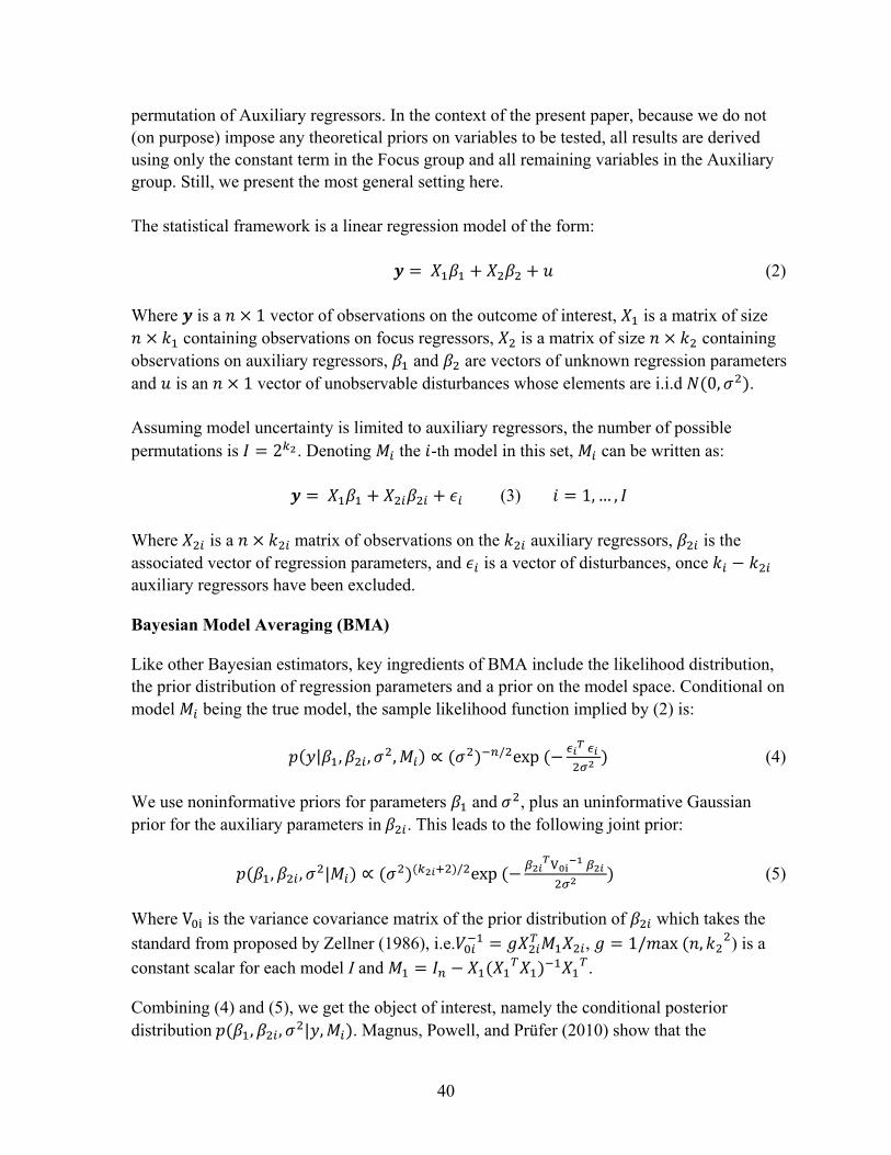
40
permutation of Auxiliary regressors. In the context of the present paper, because we do not (on purpose) impose any theoretical priors on variables to be tested, all results are derived using only the constant term in the Focus group and all remaining variables in the Auxiliary group. Still, we present the most general setting here. The statistical framework is a linear regression model of the form:
(2)
Where is a 1 vector of observations on the outcome of interest, is a matrix of size
containing observations on focus regressors, is a matrix of size containing observations on auxiliary regressors, and are vectors of unknown regression parameters and is an 1 vector of unobservable disturbances whose elements are i.i.d 0, . Assuming model uncertainty is limited to auxiliary regressors, the number of possible permutations is 2 . Denoting the -th model in this set, can be written as:
(3) 1,… , Where is a matrix of observations on the auxiliary regressors, is the associated vector of regression parameters, and is a vector of disturbances, once auxiliary regressors have been excluded.
Bayesian Model Averaging (BMA)
Like other Bayesian estimators, key ingredients of BMA include the likelihood distribution, the prior distribution of regression parameters and a prior on the model space. Conditional on model being the true model, the sample likelihood function implied by (2) is:
| , , , / exp (4)
We use noninformative priors for parameters and , plus an uninformative Gaussian prior for the auxiliary parameters in . This leads to the following joint prior:
, , | / exp V (5)
Where V is the variance covariance matrix of the prior distribution of which takes the
standard from proposed by Zellner (1986), i.e. , 1/ ax , ) is a
constant scalar for each model I and .
Combining (4) and (5), we get the object of interest, namely the conditional posterior distribution , , | , . Magnus, Powell, and Prüfer (2010) show that the
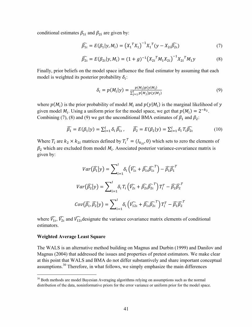
41
conditional estimates and are given by:
| , (7)
| , 1 (8)
Finally, prior beliefs on the model space influence the final estimator by assuming that each model is weighted its posterior probability :
| |
∑ | (9)
where is the prior probability of model and | is the marginal likelihood of given model . Using a uniform prior for the model space, we get that 2 . Combining (7), (8) and (9) we get the unconditional BMA estimates of and :
| ∑ , | ∑ (10)
Where are matrices defined by , 0 which sets to zero the elements of
which are excluded from model . Associated posterior variance-covariance matrix is given by:
,
where , and designate the variance covariance matrix elements of conditional estimators.
Weighted Average Least Square
The WALS is an alternative method building on Magnus and Durbin (1999) and Danilov and Magnus (2004) that addressed the issues and properties of pretest estimators. We make clear at this point that WALS and BMA do not differ substantively and share important conceptual assumptions.30 Therefore, in what follows, we simply emphasize the main differences
30 Both methods are model Bayesian Averaging algorithms relying on assumptions such as the normal distribution of the data, noninformative priors for the error variance or uniform prior for the model space.
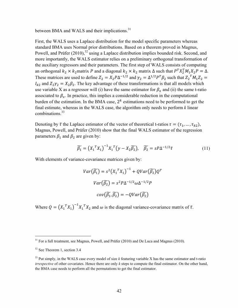
42
between BMA and WALS and their implications.31
First, the WALS uses a Laplace distribution for the model specific parameters whereas standard BMA uses Normal prior distributions. Based on a theorem proved in Magnus, Powell, and Prüfer (2010),32 using a Laplace distribution implies bounded risk. Second, and more importantly, the WALS estimator relies on a preliminary orthogonal transformation of the auxiliary regressors and their parameters. The first step of WALS consists of computing an orthogonal matrix and a diagonal matrix ∆ such that ∆. These matrices are used to define ∆ / and ∆ / such that
and . The key advantage of these transformations is that all models which use variable X as a regressor will (i) have the same estimator for and (ii) the same t-ratio associated to . In practice, this implies a considerable reduction in the computational burden of the estimation. In the BMA case, 2 estimations need to be performed to get the final estimate, whereas in the WALS case, the algorithm only needs to perform k linear combinations.33
Denoting by the Laplace estimator of the vector of theoretical t-ratios , … , , Magnus, Powell, and Prüfer (2010) show that the final WALS estimator of the regression parameters and are given by:
, ∆ / (11)
With elements of variance-covariance matrices given by:
∆ / ∆ /
,
Where and is the diagonal variance-covariance matrix of .
31 For a full treatment, see Magnus, Powell, and Prüfer (2010) and De Luca and Magnus (2010).
32 See Theorem 1, section 3.4
33 Put simply, in the WALS case every model of size k featuring variable X has the same estimator and t-ratio irrespective of other covariates. Hence there are only k steps to compute the final estimator. On the other hand, the BMA case needs to perform all the permutations to get the final estimator.
43
Criteria for Significance and Interpretation
An important aspect to clarify is the issue of significance criteria. How to determine, ex post, that a regressor is robustly correlated to the LHS variable—here a growth slowdown?
In the BMA case, Masanjala and Papageorgiou (2008) suggest that a posterior inclusion probability (PIP) above 0.5—which corresponds approximately to a t-ratio of 1—indicates a robust regressor. We use the same threshold when sorting out variables according to their PIPs in the different modules. The argument behind this choice follows from the assumptions of the model: when the size of the model is unknown and researchers are strongly agnostic about the actual or “true” model space—the stance adopted in this paper—a standard procedure is to assume a uniform distribution over the model space, implying that every model (from size 1 to k) has the same chance of being selected. In such case, the prior probability of including any regressor to be selected ex-ante is 0.5. After computation of the model however, if the PIP rises above the prior inclusion probability, there is a support for including this variable. By contrast a value below the prior probability implies omission.
Two points are worth noting. First, because the PIP is a function of the likelihood of models including variable X, it increases if models featuring variable X are more likely than others. Second, the explanation above makes it clear that there is no “commonly” adopted threshold to rule about significance and therefore that comparing prima facie PIPs across papers is irrelevant. Criteria differ across studies because prior inclusion probabilities also differ.34
In the WALS case, the counterparts of these Bayesian quantities (the PIPs) cannot be computed.35 Magnus, Powell, and Prüfer (2010) suggest an absolute value of the t-ratio greater than 1 for a variable to qualify as robust. This choice is motivated by two arguments. First, consider for simplicity the simple regression model where k 1. 36 Removing auxiliary variable 2 from the model implies an increase in the . However, the adjusted will decrease if, and only if, the t-ratio of the auxiliary parameter is smaller than one in absolute value. Second, Magnus and Durbin (1999) also show37 that if we
define the ‘theoretical’ t-ratio as τ β
σ/ X ′M X then , if, and only
if, | τ |≤1, where denotes the restricted (with 0) estimator and the unrestricted
34 An illustration is Sala-i-Martin, Dopplehofer, and Miller (2004) who use a “lower” threshold (0.104) to decide whether a variable is robust or not. However, this PIP threshold is simply a consequence of the authors’ choice to penalize models with a high number of parameters.
35 WALS estimators are biased and their distribution is not Gaussian.
36 so that there is only one auxiliary regressor , and only one auxiliary parameter β2.
37 See Theorem 1.
44
estimator of respectively.
The intuitive conclusion is that including variable 2 implies an increase in model fit (as measure by the adjusted R2) and improves the precision of the estimators of focus regressors (measured by a lower MSE) if and only if the t ratio of the additional regressor, in absolute value, is greater than 1. Following this argument, Magnus, Powell, and Prüfer (2010) set the benchmark for prior distributions of model parameters such that their t-ratio is one. Hence, if this t-ratio happens to be greater than 1 in after estimation, it qualifies as a robust regressor.
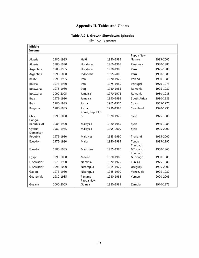
45
Appendix II. Tables and Charts
Table A.2.1. Growth Slowdowns Episodes (By income group)
Middle Income
Algeria 1980-1985 Haiti 1980-1985 Papua New Guinea 1995-2000
Algeria 1985-1990 Honduras 1960-1965 Paraguay 1980-1985
Argentina 1980-1985 Honduras 1980-1985 Peru 1975-1980
Argentina 1995-2000 Indonesia 1995-2000 Peru 1980-1985
Belize 1990-1995 Iran 1970-1975 Poland 1980-1985
Bolivia 1975-1980 Iran 1975-1980 Portugal 1970-1975
Botswana 1975-1980 Iraq 1980-1985 Romania 1975-1980
Botswana 2000-2005 Jamaica 1970-1975 Romania 1980-1985
Brazil 1975-1980 Jamaica 1990-1995 South Africa 1980-1985
Brazil 1980-1985 Jordan 1965-1970 Spain 1965-1970
Bulgaria 1980-1985 Jordan 1980-1985 Swaziland 1990-1995
Chile 1995-2000 Korea, Republic of 1970-1975 Syria 1975-1980
Congo, Republic of 1985-1990 Malaysia 1980-1985 Syria 1980-1985
Cyprus 1980-1985 Malaysia 1995-2000 Syria 1995-2000 Dominican Republic 1975-1980 Maldives 1985-1990 Thailand 1995-2000
Ecuador 1975-1980 Malta 1980-1985 Tonga 1985-1990
Ecuador 1980-1985 Mauritius 1975-1980 Trinidad &Tobago 1960-1965
Egypt 1995-2000 Mexico 1980-1985 Trinidad &Tobago 1980-1985
El Salvador 1975-1980 Namibia 1970-1975 Tunisia 1975-1980
El Salvador 1995-2000 Nicaragua 1965-1970 Uruguay 1995-2000
Gabon 1975-1980 Nicaragua 1985-1990 Venezuela 1975-1980
Guatemala 1980-1985 Panama 1980-1985 Yemen 2000-2005
Guyana 2000-2005 Papua New Guinea 1980-1985 Zambia 1970-1975
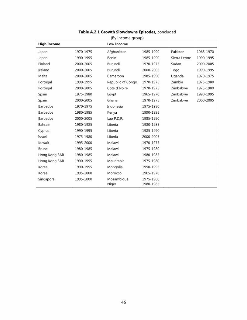
46
Table A.2.1 Growth Slowdowns Episodes, concluded (By income group)
High Income Low Income
Japan 1970-1975 Afghanistan 1985-1990 Pakistan 1965-1970
Japan 1990-1995 Benin 1985-1990 Sierra Leone 1990-1995
Finland 2000-2005 Burundi 1970-1975 Sudan 2000-2005
Ireland 2000-2005 Burundi 2000-2005 Togo 1990-1995
Malta 2000-2005 Cameroon 1985-1990 Uganda 1970-1975
Portugal 1990-1995 Republic of Congo 1970-1975 Zambia 1975-1980
Portugal 2000-2005 Cote d`Ivoire 1970-1975 Zimbabwe 1975-1980
Spain 1975-1980 Egypt 1965-1970 Zimbabwe 1990-1995
Spain 2000-2005 Ghana 1970-1975 Zimbabwe 2000-2005
Barbados 1970-1975 Indonesia 1975-1980
Barbados 1980-1985 Kenya 1990-1995
Barbados 2000-2005 Lao P.D.R. 1985-1990
Bahrain 1980-1985 Liberia 1980-1985
Cyprus 1990-1995 Liberia 1985-1990
Israel 1975-1980 Liberia 2000-2005
Kuwait 1995-2000 Malawi 1970-1975
Brunei 1980-1985 Malawi 1975-1980
Hong Kong SAR 1980-1985 Malawi 1980-1985
Hong Kong SAR 1990-1995 Mauritania 1975-1980
Korea 1990-1995 Mongolia 1990-1995
Korea 1995-2000 Morocco 1965-1970
Singapore 1995-2000 Mozambique 1975-1980 Niger 1980-1985
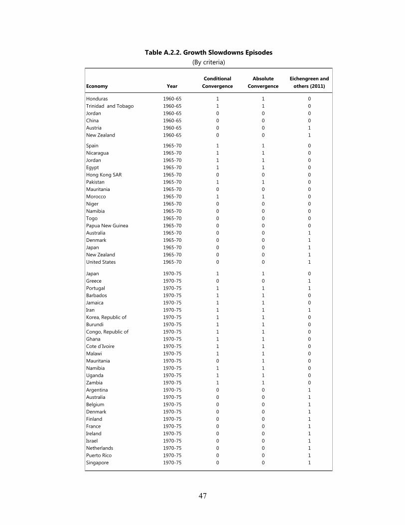
47
Table A.2.2. Growth Slowdowns Episodes (By criteria)
Economy YearConditional
ConvergenceAbsolute
ConvergenceEichengreen and
others (2011)
Honduras 1960-65 1 1 0Trinidad and Tobago 1960-65 1 1 0Jordan 1960-65 0 0 0China 1960-65 0 0 0Austria 1960-65 0 0 1New Zealand 1960-65 0 0 1
Spain 1965-70 1 1 0Nicaragua 1965-70 1 1 0Jordan 1965-70 1 1 0Egypt 1965-70 1 1 0Hong Kong SAR 1965-70 0 0 0Pakistan 1965-70 1 1 0Mauritania 1965-70 0 0 0Morocco 1965-70 1 1 0Niger 1965-70 0 0 0Namibia 1965-70 0 0 0Togo 1965-70 0 0 0Papua New Guinea 1965-70 0 0 0Australia 1965-70 0 0 1Denmark 1965-70 0 0 1Japan 1965-70 0 0 1New Zealand 1965-70 0 0 1United States 1965-70 0 0 1
Japan 1970-75 1 1 0Greece 1970-75 0 0 1Portugal 1970-75 1 1 1Barbados 1970-75 1 1 0Jamaica 1970-75 1 1 0Iran 1970-75 1 1 1Korea, Republic of 1970-75 1 1 0Burundi 1970-75 1 1 0Congo, Republic of 1970-75 1 1 0Ghana 1970-75 1 1 0Cote d`Ivoire 1970-75 1 1 0Malawi 1970-75 1 1 0Mauritania 1970-75 0 1 0Namibia 1970-75 1 1 0Uganda 1970-75 1 1 0Zambia 1970-75 1 1 0Argentina 1970-75 0 0 1Australia 1970-75 0 0 1Belgium 1970-75 0 0 1Denmark 1970-75 0 0 1Finland 1970-75 0 0 1France 1970-75 0 0 1Ireland 1970-75 0 0 1Israel 1970-75 0 0 1Netherlands 1970-75 0 0 1Puerto Rico 1970-75 0 0 1Singapore 1970-75 0 0 1
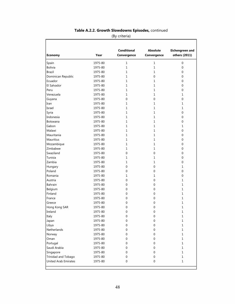
48
Table A.2.2. Growth Slowdowns Episodes, continued (By criteria)
Economy YearConditional
ConvergenceAbsolute
ConvergenceEichengreen and
others (2011)
Spain 1975-80 1 1 0Bolivia 1975-80 1 1 0Brazil 1975-80 1 1 0Dominican Republic 1975-80 1 0 0Ecuador 1975-80 1 1 0El Salvador 1975-80 1 1 0Peru 1975-80 1 1 0Venezuela 1975-80 1 1 1Guyana 1975-80 0 0 0Iran 1975-80 1 1 1Israel 1975-80 1 1 1Syria 1975-80 1 1 0Indonesia 1975-80 1 1 0Botswana 1975-80 1 1 0Gabon 1975-80 1 1 1Malawi 1975-80 1 1 0Mauritania 1975-80 1 1 0Mauritius 1975-80 1 1 0Mozambique 1975-80 1 1 0Zimbabwe 1975-80 1 1 0Swaziland 1975-80 0 0 0Tunisia 1975-80 1 1 0Zambia 1975-80 1 1 0Hungary 1975-80 0 0 1Poland 1975-80 0 0 0Romania 1975-80 1 1 0Austria 1975-80 0 0 1Bahrain 1975-80 0 0 1Belgium 1975-80 0 0 1Finland 1975-80 0 0 1France 1975-80 0 0 1Greece 1975-80 0 0 1Hong Kong SAR 1975-80 0 0 1Ireland 1975-80 0 0 1Italy 1975-80 0 0 1Japan 1975-80 0 0 1Libya 1975-80 0 0 1Netherlands 1975-80 0 0 1Norway 1975-80 0 0 1Oman 1975-80 0 0 1Portugal 1975-80 0 0 1Saudi Arabia 1975-80 0 0 1Singapore 1975-80 0 0 1Trinidad and Tobago 1975-80 0 0 1United Arab Emirates 1975-80 0 0 1
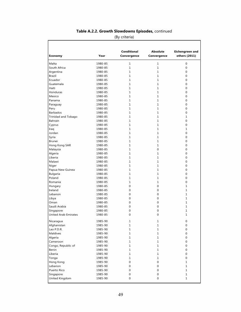
49
Table A.2.2. Growth Slowdowns Episodes, continued (By criteria)
Economy YearConditional
ConvergenceAbsolute
ConvergenceEichengreen and
others (2011)
Malta 1980-85 1 1 0South Africa 1980-85 1 1 0Argentina 1980-85 1 1 0Brazil 1980-85 1 1 0Ecuador 1980-85 1 1 0Guatemala 1980-85 1 1 0Haiti 1980-85 1 1 0Honduras 1980-85 1 1 0Mexico 1980-85 1 1 0Panama 1980-85 1 1 0Paraguay 1980-85 1 1 0Peru 1980-85 1 1 0Barbados 1980-85 1 1 0Trinidad and Tobago 1980-85 1 1 1Bahrain 1980-85 1 1 0Cyprus 1980-85 1 1 0Iraq 1980-85 1 1 1Jordan 1980-85 1 1 0Syria 1980-85 1 1 0Brunei 1980-85 1 1 0Hong Kong SAR 1980-85 1 1 0Malaysia 1980-85 1 0 0Algeria 1980-85 1 1 0Liberia 1980-85 1 1 0Malawi 1980-85 1 1 0Niger 1980-85 1 1 0Papua New Guinea 1980-85 1 1 0Bulgaria 1980-85 1 1 0Poland 1980-85 1 1 0Romania 1980-85 1 1 0Hungary 1980-85 0 0 1Ireland 1980-85 0 0 1Lebanon 1980-85 0 0 1Libya 1980-85 0 0 1Oman 1980-85 0 0 1Saudi Arabia 1980-85 0 0 1Singapore 1980-85 0 0 1United Arab Emirates 1980-85 0 0 1
Nicaragua 1985-90 1 1 0Afghanistan 1985-90 1 1 0Lao P.D.R. 1985-90 1 1 0Maldives 1985-90 1 1 0Algeria 1985-90 1 1 0Cameroon 1985-90 1 1 0Congo, Republic of 1985-90 1 1 0Benin 1985-90 1 1 0Liberia 1985-90 1 1 0Tonga 1985-90 1 1 0Hong Kong 1985-90 0 0 1Lebanon 1985-90 0 0 1Puerto Rico 1985-90 0 0 1Singapore 1985-90 0 0 1United Kingdom 1985-90 0 0 1
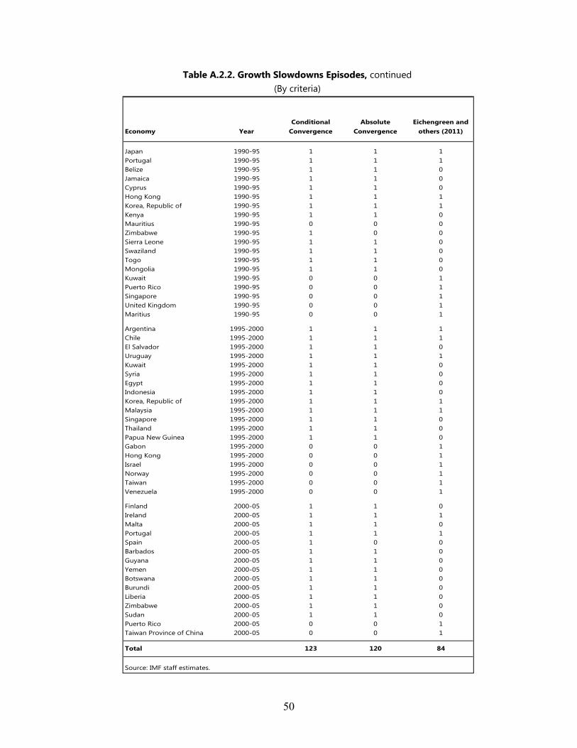
50
Table A.2.2. Growth Slowdowns Episodes, continued (By criteria)
Economy YearConditional
ConvergenceAbsolute
ConvergenceEichengreen and
others (2011)
Japan 1990-95 1 1 1Portugal 1990-95 1 1 1Belize 1990-95 1 1 0Jamaica 1990-95 1 1 0Cyprus 1990-95 1 1 0Hong Kong 1990-95 1 1 1Korea, Republic of 1990-95 1 1 1Kenya 1990-95 1 1 0Mauritius 1990-95 0 0 0Zimbabwe 1990-95 1 0 0Sierra Leone 1990-95 1 1 0Swaziland 1990-95 1 1 0Togo 1990-95 1 1 0Mongolia 1990-95 1 1 0Kuwait 1990-95 0 0 1Puerto Rico 1990-95 0 0 1Singapore 1990-95 0 0 1United Kingdom 1990-95 0 0 1Maritius 1990-95 0 0 1
Argentina 1995-2000 1 1 1Chile 1995-2000 1 1 1El Salvador 1995-2000 1 1 0Uruguay 1995-2000 1 1 1Kuwait 1995-2000 1 1 0Syria 1995-2000 1 1 0Egypt 1995-2000 1 1 0Indonesia 1995-2000 1 1 0Korea, Republic of 1995-2000 1 1 1Malaysia 1995-2000 1 1 1Singapore 1995-2000 1 1 0Thailand 1995-2000 1 1 0Papua New Guinea 1995-2000 1 1 0Gabon 1995-2000 0 0 1Hong Kong 1995-2000 0 0 1Israel 1995-2000 0 0 1Norway 1995-2000 0 0 1Taiwan 1995-2000 0 0 1Venezuela 1995-2000 0 0 1
Finland 2000-05 1 1 0Ireland 2000-05 1 1 1Malta 2000-05 1 1 0Portugal 2000-05 1 1 1Spain 2000-05 1 0 0Barbados 2000-05 1 1 0Guyana 2000-05 1 1 0Yemen 2000-05 1 1 0Botswana 2000-05 1 1 0Burundi 2000-05 1 1 0Liberia 2000-05 1 1 0Zimbabwe 2000-05 1 1 0Sudan 2000-05 1 1 0Puerto Rico 2000-05 0 0 1Taiwan Province of China 2000-05 0 0 1
Total 123 120 84
Source: IMF staff estimates.

51
Note: The procedure in Eichengreen, Park, and Shin (2012) identifies strings of consecutive years as growth slowdowns. We matched them with our five-year panel using the following rule. With t denoting the year of a slowdown identified in Eichengreen, Park, and Shin (2012) and , 1…12, the five-year panel dimension used above, then:
if 2 t 2 then the slowdown is imputed to the period
if 3 t 2 then the slowdown is imputed to the period
if 3 t 2 then the slowdown is imputed to the period
For instance, slowdowns over the period 2000–05 reported in the right column include slowdowns that started in 1998, 1999, 2000, 2001 and 2002 according to Eichengreen, Park, and Shin (2012). However, slowdowns that started between 1993 and 1997 are counted as 1995–2000 slowdowns, whereas those who started between 2003 and 2007 are imputed to 2005–10. Note that this rule implies that a string of consecutive years can also be imputed to 2 consecutive periods in our five-year panel dimension.

52
Table A.2.3. Independent Variables: Unit and Sources
1 Regulation refers to credit market, labor market, and business regulations. Of the six subindices covering labor market regulations, only the three that are not taken from the Employing Workers Index of the World Bank’s Doing Business database are considered.
Descriptions Sources Category Start End Frequency
Fertility rate, total (births per woman) WDI Demography 1960 2009 AnnualDependency ratio United Nations Demography 1950 2005 5-year Sex ratio United Nations Demography 1950 2005 5-yearAgriculture share of value added (percent of GDP) WDI Economic Structure 1970 2011 AnnualServices share of value added (percent of GDP) WDI Economic Structure 1970 2011 AnnualIndustry share value added (percent of GDP) WDI Economic Structure 1970 2011 AnnualOutput diversification Papageorgiou and Spatafora (2012) Economic Structure 2000 2010 AnnualTelephone lines Calderon and Serven (2004); WDI Infrastructure 1960 2010 5-yearPower (generating capacity) Calderon and Serven (2004); WDI Infrastructure 1960 2010 5-yearRoads Calderon and Serven (2004); WDI Infrastructure 1960 2010 5-yearSize of government Economic Freedom dataset Institutions 1960 2010 5-yearRule of law Economic Freedom dataset Institutions 1960 2010 5-yearFreedom to trade internationally Economic Freedom dataset Institutions 1960 2010 5-yearRegulation1 Economic Freedom dataset Institutions 1960 2010 5-yearFinancial openness Chinn and Ito (2006) Institutions 1970 2009 AnnualGross capital inflows as percentage of GDP World Economic Outlook MACRO 1970 2009 AnnualGross capital outflows as percentage of GDP World Economic Outlook MACRO 1970 2009 AnnualBanking crisis dummy Laeven and Valencia (2012) MACRO 1975 2008 AnnualReal exchange rate IMF staff calculations MACRO 1950 2009 AnnualTrade openness at 2005 constant prices (percent) PWT MACRO 1950 2009 AnnualCPI inflation WDI MACRO 1970 2010 AnnualPrice level of investment PWT MACRO 1950 2009 AnnualExternal debt (net) to GDP ratio Lane and Milesi Ferretti MACRO 1970 2010 AnnualPublic debt to GDP ratio Abbas and others (2010) MACRO 1950 2010 AnnualTerms of trade World Economic Outlook MACRO 1970 2009 AnnualReserves/GDP ratio World Economic Outlook MACRO 1970 2010 AnnualInvestment share of PPP GDP per capita at 2005 constant PWT MACRO 1960 2010 AnnualOil exporters' price shock IMF staff calculations MACRO 1950 2010 AnnualFood exporters' price shock IMF staff calculations MACRO 1950 2010 AnnualOil importers' price shock IMF staff calculations MACRO 1950 2010 AnnualFood importers' price shock IMF staff calculations MACRO 1950 2010 AnnualFraction of country in tropics Sala-i-martin and others (2004) Other 1950 2010 AnnualSpanish colony Sala-i-martin and others (2004) Other 1950 2010 AnnualFraction Buddhist Sala-i-martin and others (2004) Other 1950 2010 AnnualEthno linguistic fractionalization Sala-i-martin and others (2004) Other 1950 2010 AnnualWar and civil conflicts Correlates of War Project Other 1950 2010 AnnualNatural disaster International Disaster Database Other 1950 2010 AnnualDistance (GDP weighted) World Bank TRADE 1950 2010 AnnualRegional integration IMF staff calculations TRADE 1960 2010 AnnualTrade diversification - Theil Index Papageorgiou and Spatafora (2012) TRADE 1960 2010 Annual
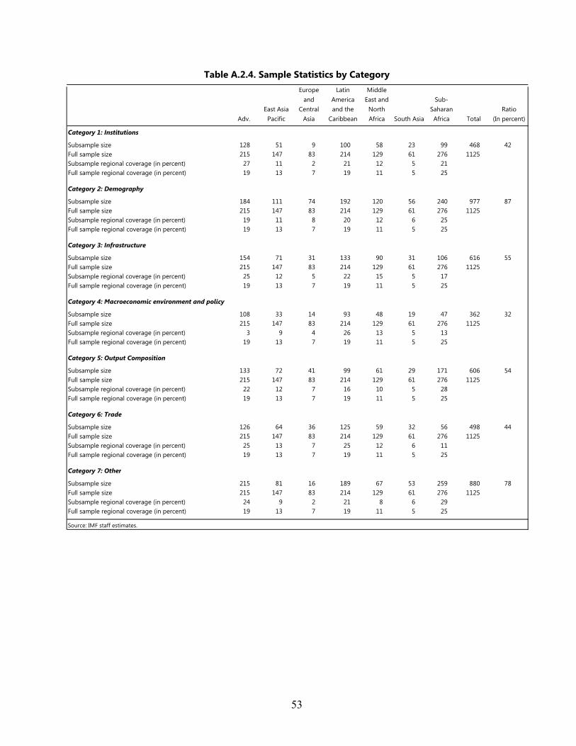
53
Table A.2.4. Sample Statistics by Category
Adv.East Asia Pacific
Europe and
Central Asia
Latin America and the
Caribbean
Middle East and
North Africa South Asia
Sub-Saharan Africa Total
Ratio (In percent)
Category 1: Institutions
Subsample size 128 51 9 100 58 23 99 468 42Full sample size 215 147 83 214 129 61 276 1125Subsample regional coverage (in percent) 27 11 2 21 12 5 21Full sample regional coverage (in percent) 19 13 7 19 11 5 25
Category 2: Demography
Subsample size 184 111 74 192 120 56 240 977 87Full sample size 215 147 83 214 129 61 276 1125Subsample regional coverage (in percent) 19 11 8 20 12 6 25Full sample regional coverage (in percent) 19 13 7 19 11 5 25
Category 3: Infrastructure
Subsample size 154 71 31 133 90 31 106 616 55Full sample size 215 147 83 214 129 61 276 1125Subsample regional coverage (in percent) 25 12 5 22 15 5 17Full sample regional coverage (in percent) 19 13 7 19 11 5 25
Category 4: Macroeconomic environment and policy
Subsample size 108 33 14 93 48 19 47 362 32Full sample size 215 147 83 214 129 61 276 1125Subsample regional coverage (in percent) 3 9 4 26 13 5 13Full sample regional coverage (in percent) 19 13 7 19 11 5 25
Category 5: Output Composition
Subsample size 133 72 41 99 61 29 171 606 54Full sample size 215 147 83 214 129 61 276 1125Subsample regional coverage (in percent) 22 12 7 16 10 5 28Full sample regional coverage (in percent) 19 13 7 19 11 5 25
Category 6: Trade
Subsample size 126 64 36 125 59 32 56 498 44Full sample size 215 147 83 214 129 61 276 1125Subsample regional coverage (in percent) 25 13 7 25 12 6 11Full sample regional coverage (in percent) 19 13 7 19 11 5 25
Category 7: Other
Subsample size 215 81 16 189 67 53 259 880 78Full sample size 215 147 83 214 129 61 276 1125Subsample regional coverage (in percent) 24 9 2 21 8 6 29Full sample regional coverage (in percent) 19 13 7 19 11 5 25
Source: IMF staff estimates.

Appendix A.2.5. Composition of Regions Regions are constructed as follows: Advanced: Australia, Austria, Belgium, Canada, Denmark, Finland, France, Germany,
Greece, Iceland, Ireland, Italy, Japan, Luxembourg, Netherlands, New Zealand, Norway, Portugal, Spain, Sweden, Switzerland, Turkey, United Kingdom, and the United States.
East Asia and Pacific: Brunei, Cambodia, China, Fiji, Hong Kong SAR, Indonesia, Republic of Korea, Lao P.D.R., Malaysia, Mongolia, Papua New Guinea, Philippines, Singapore, Taiwan Province of China, Thailand, Tonga, and Vietnam.
Europe and Central Asia: Albania, Armenia, Bulgaria, Croatia, Czech Republic, Estonia, Hungary, Kazakhstan, Kyrgyzstan, Lithuania, Poland, Romania, Russia, Slovak Republic, Slovenia, Tajikistan, and Ukraine.
Latin America and the Caribbean: Argentina, Barbados, Belize, Bolivia, Brazil, Chile, Colombia, Costa Rica, Dominican Republic, Ecuador, El Salvador, Guatemala, Guyana, Haiti, Honduras, Jamaica, Mexico, Nicaragua, Panama, Paraguay, Peru, Trinidad &Tobago, Uruguay, and Venezuela
Middle East and North Africa: Algeria, Bahrain, Cyprus, Egypt, Iran, Iraq, Israel, Jordan, Kuwait, Libya, Malta, Morocco, Qatar, Saudi Arabia, Syria, Tunisia, United Arab Emirates, and Yemen.
South Asia: Afghanistan, Bangladesh, India, Maldives, Nepal, Pakistan, Sri Lanka
Sub-Saharan Africa: Benin, Botswana, Burundi, Cameroon, Central African Republic, Congo, Republic of, Cote d`Ivoire, Gabon, Gambia, Ghana, Kenya, Lesotho, Liberia, Malawi, Mali, Mauritania, Mauritius, Mozambique, Namibia, Niger, Rwanda, Senegal, Sierra Leone, South Africa, Sudan, Swaziland, Tanzania, Togo, Uganda, Zambia, and Zimbabwe.
55
REFERENCES
Abiad, A., J. Bluedorn, J. Guajardo, and P. Topalova, 2012, World Economic Outlook
(Washington: International Monetary Fund, October). Abu-Ghaida, D. and S. Klasen, 2004, “The Costs of Missing the Millennium Development
Goal on Gender Equity,” World Development, Elsevier, Vol. 32, No. 7, pp. 1075‒1107. Abdon, A, J. Felipe and U. Kumar, 2012, “Tracking the Middle-Income Trap: What Is It,
Who Is in It, and Why?” Levy Economics Institute of Bard College Working Paper 715, April (Annandale-on-Hudson: Levy Economics Institute of Bard College)
Aghion, P., N. Bloom, R. Blyundell, R. Griffith, and P. Howitt, 2005, “Competition and
Innovation: An Inverted U Relationship,” Quarterly Journal of Economics, pp. 70128. Agenor, P., and Canuto, O., 2012. “Middle-Income Growth Traps,” Policy Research
Working Paper Series 6210 (Washington: World Bank). Aiyar, S., 2011, “How Did the Crisis in International Funding Markets Affect Bank Lending?
Balance Sheet Evidence from the UK,” Bank of England Working Paper, No. 424 (London: Bank of England).
Aiyar, S., 2012, “From Financial Crisis to Great Recession: The Role of Globalized Banks,”
American Economic Review, Vol. 102, No. 3, pp. 225–30. Aiyar, S. and C-J. Dalgaard, 2005, “Total Factor Productivity Revisited: A Dual Approach to
Development Accounting,” IMF Staff Papers, Vol. 52, pp. 88–102 (Washington: International Monetary Fund).
Aiyar, S., and C-J. Dalgaard, 2009, “Accounting for Productivity: Is it OK to Assume that
the World is Cobb-Douglas?” Journal of Macroeconomics, Vol. 31, No. 2, pp. 290‒303. Aiyar, S. and A. Mody, 2011, “The Demographic Dividend: Evidence from the Indian
States?” IMF Working Paper 11/38 (Washington: International Monetary Fund). Aiyar, S., 2011, “How Did the Crisis in International Funding Markets Affect Bank Lending?
Balance Sheet Evidence from the UK,” Bank of England Working Paper, No. 424 (London: Bank of England).
Agenor, P.R. and O. Canuto, 2012, “Middle-Income Growth Traps,” Policy Research
Working Paper Series 6210 (Washington: World Bank).
56
Aghion, P., N. Bloom, R. Blyundell, R. Griffith and P. Howitt, 2005), “Competition and Innovation: an Inverted U Relationship,” Quarterly Journal of Economics, pp. 701‒28.
Agosin, M., 2007, “Export Diversification and Growth in Emerging Economies,” Working
Papers 233 (Santiago: University of Chile, Department of Economics). Anand, R., S. Mishra, and N. Spatafora, 2012, “Structural Transformation and the
Sophistication of Production,” IMF Working Paper 12/59 (Washington: International Monetary Fund).
Bah, E., 2011, “Structural Transformation Paths across Countries,” Emerging Markets
Finance and Trade, M.E. Sharpe, Inc., Vol. 47, (May), pp. 5‒19. Barro, R. and X.Sala-i-Martin, 1991, “Convergence Across States and Regions,” Brookings
Papers on Economic Activity, Economic Studies Program, Vol. 22, No. 1, pp. 107‒182. Ben-David, D., 1993, “Equalizing Exchange: Trade Liberalization and Income
Convergence,” Quarterly Journal of Economics, MIT Press, Vol. 108 (August), No. 3, pp. 653–79.
Ben-David, D., and D. Papell, 1998, “Slowdowns and Meltdowns: Postwar Growth Evidence
from 74 Countries,” Review of Economics and Statistics, MIT Press, Vol. 80 (November), No. 4, pp. 561–71.
Berg, A., Ostry, J. and J. Zettelmeyer, 2012, “What Makes Growth Sustained?” Journal of
Development Economics, Vol. 98, No. 2, pp. 149–66 (Amsterdam: Elsevier) Bils, M., and P. Klenow, 2000, “Does Schooling Cause Growth?” American Economic
Review, Vol. 90 (December), No. 5, pp. 1160–83. Bloom, D., and J. Williamson, 1998, “Demographic Transitions and Economic Miracles in
Emerging Asia,” World Bank Economic Review, Oxford University Press, Vol. 12 (September), No. 3, pp. 419–55.
Bloom, D., D. Canning, and P. Malaney, 2000, “Demographic Change and Economic
Growth in Asia.” Population and Development Review, Vol. 26, pp. 257–90. Bloom, D. and D. Canning, 2004, “Global Demographic Change: Dimensions and Economic
Significance,” in Global Demographic Change: Economic Impacts and Policy Challenges, proceedings of a symposium, sponsored by the Federal Reserve Bank of Kansas City, Jackson Hole, Wyoming, August 26–28, pp. 9–56.
57
Boulhol, H. and A. Serres, 2010, “Have Developed Countries Escaped the Curse of Distance?” Journal of Economic Geography, Oxford University Press, Vol. 10 (January), No. 1, pp. 113–39.
Brock, W., and S.N. Durlauf, 2001, “Growth Empirics and Reality,” World Bank Economic
Review, Vol. 15, No. 2, pp. 229–72. Bruno, M. and W. Easterly, 1998, “Inflation Crises and Long-Run Growth,” Journal of
Monetary Economics, Elsevier, Vol. 41 (February), No. 1, pp. 3–26. Buchanan, J. and G. Tullock, 1962, “The Calculus of Consent: Logical Foundations of
Constitutional Democracy” (Ann Arbor: University of Michigan Press). Bussière, M., and M. Fratzscher, 2008 “Financial Openness and Growth: Short-Run Gain,
Long-Run Pain?” Review of International Economics, Vol. 16, No. 1, pp. 69–95. Cerra, V., and S. Saxena, 2008, “Growth Dynamics: The Myth of Economic Recovery,”
American Economic Review, Vol. 98, No. 1, pp. 439–57. Calderon, C. and L. Serven, 2004, “The Effects of Infrastructure Development on Growth
and Income Distribution,” Policy Research Working Paper Series 3400 (Washington: World Bank).
Caselli, F., G. Esquivel, and F. Lefort, 1996, “Reopening the Convergence Debate: A New
Look at Cross-Country Growth Empirics,” Journal of Economic Growth, Springer, Vol. 1 (September), No. 3, pp. 363–89.
Chen H., A. Mirestean, and C. Tsangarides, 2009, “Limited Information Bayesian Model
Averaging for Dynamic Panels with Short Time Periods,” IMF Working Paper 09/74. Chinn, M., and H. Ito, 2006, “What Matters for Financial Development? Capital Controls,
Institutions, and Interactions,” Journal of Development Economics, Elsevier, Vol. 81, (October), No. 1, pp. 163–92.
Cetorelli, N. and L. Goldberg, 2011, “Global Banks and International Shock Transmission:
Evidence from the Crisis,” IMF Economic Review, Palgrave Macmillan, Vol. 59 (April), No. 1, pp. 41–76.
Danilov, D., J.R. Magnus, 2004, “On the Harm That Ignoring Pretesting Can Cause,”
Journal of Econometrics, Vol. 122, p. 2746. De Long, J., and A. Shleifer, 1993, “Princes and Merchants: European City Growth before
58
the Industrial Revolution,” Journal of Law and Economics, Vol. 36 (October), No. 2, pp. 671‒702.
De Luca, G. and J.R. Magnus, 2011, “Bayesian Model Averaging and Weighted Average
Least Squares: Equivariance, Stability, and Numerical Issues,” The Stata Journal, Vol. 11, pp. 518–44.
Demetriades, P., and T. Mamuneas, 2000, “Intertemporal Output and Employment Effects of
Public Infrastructure Capital: Evidence from 12 OECD Economics,” Economic Journal, Royal Economic Society, Vol. 110 (July), No. 465, pp. 687–712.
Durlauf, S.N., P.A. Johnson and J.R.W. Temple, 2005, “Growth Econometrics,” in
Handbook of Economic Growth, ed. by P. Aghion and S.N. Durlauf, pp. 555–677 (North Holland, Amsterdam).
Durlauf, S.N., A. Kourtellos, and C.M. Tan, 2008, “Are Any Growth Theories Robust?”
Economic Journal, Vol. 118, No. 527, pp. 329–46. Durlauf, S.N., A. Kourtellos and C. Tan, 2009, “Are any Growth Theories Robust?”
Economic Journal, Royal Economic Society, Vol. 118 (March), No. 527, pp. 329–46. Duval, R. and C. Maisonneuve, 2010, “Long-Run Growth Scenarios for the World
Economy,” Journal of Policy Modeling, Vol. 32, pp. 64–80. Easterly, W., M. Kremer, L. Pritchett, and L. Summers, 1993, “Good Policy or Good Luck?
Country Growth Performance and Temporary Shocks,” Journal of Monetary Economics, Vol. 32, pp. 459–83.
Easterly, W, and R. Levine, 1997, “Africa's Growth Tragedy: Policies and Ethnic Divisions,”
Quarterly Journal of Economics, MIT Press, Vol. 112, No. 4, pp. 1203–50 (November). Edwards, S., 2001, “Capital Mobility and Economic Performance: Are Emerging Economies
Different?” NBER Working Papers 8076 (Cambridge, Massachusetts: National Bureau of Economic Research).
Eichengreen, B., D. Park, and K. Shin, 2012, “When Fast Growing Economies Slow Down:
International Evidence and Implications for China,” Asian Economic Papers, 11, pp 42–87.
––––––––, 2013, “Growth Slowdowns Redux: New Evidence on the Middle-Income Trap,”
NBER Working Paper 18673 (Cambridge, Massachusetts: National Bureau of Economic Research).

59
Eicher T.S., A. Lenkoski A., and A.E. Raftery, 2009, “Bayesian Model Averaging and
Endogeneity under Model Uncertainty: An Application to Development Determinants” (unpublished; University of Washington).
Egert, B., T. Kozluk, and D. Sutherland, 2009, “Infrastructure and Growth: Empirical
Evidence,” William Davidson Institute Working Paper 957 (April). Fernández, C., E. Ley, and M.F.J. Steel, 2001, “Model Uncertainty in Cross-Country Growth
Regressions,” Journal of Applied Econometrics, Vol. 16, pp. 563–76. Fischer, S., 1993, “The Role of Macroeconomic Factors in Growth,” Journal of Monetary
Economics, Vol. 32, No. 3, pp. 485–512 Gaertner, M., and C. Papageorgiou, 2011, “Sustaining Tanzania’s High Growth Path
Through Exports” (Washington: International Monetary Fund). Glick, R., and M. Hutchinson, 2001, “Banking Crises and Currency Crises: How Common
Are the Twins,” in Financial Crises in Emerging Markets, ed. by R. Glick, R. Moreno, and M. Spiegel (New York: Cambridge University Press).
Gollin, D., 2002, “Getting Income Shares Right,” Journal of Political Economy, 110,
pp 458‒74. Hall, R., and C. Jones, 1999, “Why Do Some Countries Produce So Much More Output Per
Worker Than Others?” Quarterly Journal of Economics, Vol. 114, No. 1, pp. 83–116 Harding, D., and A. Pagan, 2002, “Dissecting the Cycle: A Methodological Investigation,”
Journal of Monetary Economics, Elsevier, Vol. 49 (March), No. 2, pp 365–81. Harris, J., and M. Todaro, 1970, “Migration, Unemployment and Development: A Two-
Sector Analysis,” American Economic Review, Vol. 60, No., pp. 126–42. Hausmann, R., L. Pritchett, and D. Rodrik, 2005, “Growth Accelerations,” Journal of
Economic Growth, Vol. 10 (December), No. 4, pp. 303–29. Hausmann, R., F. Rodriguez and A. Wagner, 2006, “Growth Collapses,” Center for
International Development Working Paper No. 136. Higgins, M., 1998, “Demography, National Savings, and International Capital Flows,”
International Economic Review, Vol. 39 (May) No. 2, pp. 343–69.

60
Islam, N., 1995, “Growth Empirics: A Panel Data Approach,” Quarterly Journal of Economics, MIT Press, Vol. 110 (November), No. 4, pp. 1127–70.
Im, S.K., H. Pesaran, and Y. Shin, 2003, “Testing for unit roots in heterogeneous panels,”
Journal of Econometrics, Elsevier, Vol. 115 (July), No. 1, pp. 53–74. Imbs, J., and R. Wacziarg, 2003, “Stages of Diversification,” American Economic Review,
American Economic Association, Vol. 93 (March), No. 1, pp. 63–86. Jankowska, A., A. Nagengast, and J. Perea, 2012, “The Product Space and the Middle-
Income Trap: Comparing Asian and Latin American Experiences,” OECD Development Centre Working Paper 311.
Kelley, A., and S. Schmidt, 1996, “Saving, Dependency and Development,” Journal of
Population Economics, Vol. 9, No. 4. Knack, S., and P. Keefer, 1997, “Does Social Capital Have an Economic Payoff? A Cross-
Country Investigation,” Quarterly Journal of Economics, Vol. 112, No. 4, pp. 1251‒88. Kuznets, S., 1966, “Modern Economic Growth, Rate, Structure and Spread” (New Haven and
London: Yale University Press). La Porta, R., F. Lopez-de-Silanes, A. Shleifer, and R. Vishny, 1997, “Legal Determinants of
External Finance,” Journal of Finance, American Finance Association, Vol. 52 (July), No. 3, pp. 1131–50.
La Porta, R., F. Lopez-de-Silanes, A. Shleifer and R. Vishny, 1998, “Law and Finance,”
Journal of Political Economy, University of Chicago Press, Vol. 106, No. 6, pp. 1113–55 (December).
La Porta, R., F. Lopez-de-Silanes, A. Shleifer and R. Vishny, 1999, “The Quality of
Government,” Journal of Law, Economics and Organization Vol. 15, No. 1, pp. 222‒79 (Oxford University Press. April).
Laeven, L., and P. Valencia, 2012, “Systemic Banking Crises Database: An Update,” IMF
Working Paper No. 12/163 (Washington: International Monetary Fund). Leamer, E. E., 1978, “Specification Search: Ad Hoc Inference with Nonexperimental Data”
(New York: Wiley). Kaminsky, G., and C. Reinhart, 1999, “The Twin Crises: The Causes of Banking and
Balance of Payments Problems,” American Economic Review, Vol. 89, No. 3, pp. 473–
61
500. Magnus, J.R., J. Durbin, 1999, “Estimation of Regression Coefficients of Interest
When Other Regression Coefficients Are of No Interest,” Econometrica, Vol. 67, pp. 639–43.
Magnus, J. R., O. Powell, and P. Prüfer, 2010, “A Comparison of Two Model-Averaging
Techniques with an Application to Growth Empirics,” Journal of Econometrics, Vol. 154, pp. 139–153.
Masanjala, W., and C. Papageorgiou, 2008, “Rough and Lonely Road to Prosperity: A
Reexamination of the Sources of Growth in Africa Using Bayesian Model Averaging,” Journal of Applied Econometrics Vol. 23, pp. 671–82.
Mason, A., 2001, “Population, Capital, and Labor,” Population Change and Economic
Development in East Asia: Challenges Met, Opportunities Seized, Andrew Mason, ed. (Stanford: Stanford University Press).
Masters, W., and M. McMillan, 2001, “Climate and Scale in Economic Growth,” Journal of
Economic Growth, Vol. 6 (September), No. 3, pp. 167–86. Mauro, P., 1995, “Corruption and Growth,” Quarterly Journal of Economics, MIT Press,
Vol. 110, No. 3, pp. 681–712 (August). Mendoza, E., 1997, “Terms of Trade Uncertainty and Economic Growth,” Journal of
Economic Development, Vol. 54, pp. 323–56. Milesi-Ferretti, G. and V. Grilli, 1995, “Economic Effects and Structural Determinants of
Capital Controls,” IMF Working Paper 95/31 (Washington: International Monetary Fund).
Minsky, H., 1986, “Stabilizing an Unstable Economy” (Yale University Press). Minsky, H., 1992, “The Financial Instability Hypothesis,” Jerome Levy Economics Institute
Working Paper No. 74. Mironov, M., 1995, “Corruption and Growth,” Quarterly Journal of Economics, MIT Press,
Vol. 110, No. 3, pp. 681–712 (August). Moral-Benito, E., 2011, “Dynamic Panels with Predetermined Regressors: Likelihood-Based
Estimation and Bayesian Averaging with An Application to Cross-Country Growth,” Banco de España Working Papers 1109 (Madrid: Banco de España).

62
Moral Benito, E., 2012a, “Determinants of Economic Growth: A Bayesian Panel Data
Approach,” Review of Economics and Statistics, Vol. 94, No. 2. Moral-Benito, E., 2012b, “Model Averaging in Economics: An Overview,” Banco de España
Working Paper No. 1123 (Madrid: Banco de España). North, D., 1981, “Structure and Change in Economic History” (New York: Norton &
Company). North, D., 1990, “Institutions, Institutional Change, and Economic Performance”
(Cambridge: Cambridge University Press). Ostry, J., A. Ghosh, K. Habermeier, M. Chamon, M. Qureshi, and D. Reinhart, 2010,
“Capital Inflows: The Role of Controls,” IMF Staff Position Note 10/04 (Washington: International Monetary Fund).
Prasad, E., R. Rajan, and A. Subramanian, 2007, “Foreign Capital and Economic Growth,”
NBER Working Papers 13619 (Cambridge, Massachusetts: National Bureau of Economic Research).
Pritchett, L., 1998, “Patterns of Economic Growth: Hills, Plateaus, Mountains, and Plains,”
Policy Research Working Paper Series 1947 (Washington: World Bank). Psacharopoulos, G., 1994. “Returns to Investment in Education: A Global Update,” World
Development, 22, No. 9, pp. 1325–43. Quinn, D., 1997. “The Correlates of Change in International Financial Regulation,”
American Political Science Review, Vol. 9, (September), pp. 1531–51. Raftery, A. E., 1995, “Bayesian Model Selection in Social Research,” Sociological
Methodology Vol. 25, pp. 111–63. Redding, S. and A. Venables, 2004, “Geography and Export Performance: External Market
Access and Internal Supply Capacity,” NBER Chapters, in: Challenges to Globalization: Analyzing the Economics, pp. 95-130 (Cambridge, Massachusetts: National Bureau of Economic Research).
Reinhart, C. and K. Rogoff, 2010, “Growth in a Time of Debt,” NBER Working Paper, No. 15639 (Cambridge, Massachusetts: National Bureau of Economic Research).
Romp, W. and J. de Haan, 2007, “Public Capital and Economic Growth: A Critical Survey,”

63
Perspektiven der Wirtschaftspolitik, Verein für Socialpolitik, Vol. 8, No. s1, pp. 6‒52. Roller, L., and L. Waverman, 2001, “Telecommunications Infrastructure and Economic
Development: A Simultaneous Approach.” American Economic Review, Vol. 91, No. 4, pp. 909–23.
Sachs, J. and A. Warner, 1997, “Sources of Slow Growth in African Economies,” Journal of
African Economies, Vol. 6, No. 3, pp. 335‒76. Sala-i-Martin, X., G. Dopplehofer and R. Miller, 2004, “Determinants of Long-Run Growth:
A Bayesian Averaging of Classical Estimates, BACE) Approach,” American Economic Review (September).
Schumpeter, J., 1912, The Theory of Economic Development (Cambridge: Harvard Press) Sen A., 1992, Inequality Reexamined, Oxford (Cambridge: Harvard University Press). Tenreyro, S., 2007, “On the Trade Impact of Nominal Exchange Rate Volatility,” Journal of
Development Economics, Elsevier, Vol. 82, No. 2, pp. 485–508. Tsangarides, C.G., 2004, “A Bayesian Approach to Model Uncertainty,” IMF Working Paper
04/68 (Washington: International Monetary Fund). Zellner, A., 1986, “On Assessing Prior Distributions and Bayesian Regression Analysis with
G-prior Distributions,” in Bayesian Inference and Decision Techniques: Essays in Honor of Bruno de Finetti, ed. by P.K. Goel and A. Zellner (North-Holland, Amsterdam).


