GSA Data Repository Extension Driven Right-lateral Shear in the Centennial Shear Zone Adjacent to the Eastern Snake River Plain, Idaho S.J. Payne 1 , R. McCaffrey 2 , and S.A. Kattenhorn 3 1 Idaho National Laboratory, PO Box 1625, MS 2203, Idaho Falls, ID 83415 2 Portland State University, Department of Geology, PO Box 751, Portland, OR 97207 3 University of Idaho, Department of Geological Sciences, PO Box 443022, Moscow, ID 83844 Lithosphere, 2013 (With revisions to Gravitation Potential Energy (GPE) Calculations, 2015)
Transcript
GSA Data Repository
Extension Driven Right-lateral Shear in the Centennial Shear Zone Adjacent to the
Eastern Snake River Plain, Idaho
S.J. Payne1, R. McCaffrey2, and S.A. Kattenhorn3
1Idaho National Laboratory, PO Box 1625, MS 2203, Idaho Falls, ID 83415
2Portland State University, Department of Geology, PO Box 751, Portland, OR 97207
3University of Idaho, Department of Geological Sciences, PO Box 443022, Moscow, ID
83844
Lithosphere, 2013
(With revisions to Gravitation Potential Energy (GPE) Calculations, 2015)
2
Table of Contents GPS Data ………………………………………………………...…………………………. 3 Strain Rate ..……………………………………………………...…………………………. 3 Rotation Rate Calculated from Velocity …….…...………………………………………… 4 Earthquake Fault Plane Solutions .………………...……………………………………….. 5 Block Models .……………………………………………………………………………… 8 Snake River Plain Frame of Reference ……………………………………………………. 18 Gravitation Potential Energy (GPE) Calculations …………………………………………. 20 References …………………………………………………………………………………. 25
3
GPS Data The 1994–2010 GPS surface velocity field of Payne et al. (2012) has 405 continuous and survey-mode GPS sites, which include new sites in eastern Oregon, Idaho, western Wyoming and southwestern Montana. This updated field expanded the number of GPS sites beyond those in McCaffrey et al. (2007) and Payne et al. (2008). As described in Payne et al. (2012), the daily position estimates and covariance matrices of the GPS sites were combined with ~200 global stations of the International GNSS Service (Dow et al., 2009) and between 10 (1994) and ~200 (2009) western North American stations, including some Plate Boundary Observatory (PBO) (http://www.earthscope.org/observatories/pbo) and older networks, using the recent reprocessing of the Scripps Orbit and Permanent Array Center (SOPAC) (Bock et al., 1997; ftp:garner.ucsd.edu/pub/hfiles). The velocities are determined relative to the Stable North American Reference Frame (SNARF) as discussed in Payne et al. (2012).
Strain Rate We use a weighted least-squares linear regression to calculate the strain rate (xx= 4.4 ± 2.7 x 10⁻⁹ yr-1) along Profile Line A-B at an azimuth of 114º (Fig, 3D of the manuscript) using observed velocities and distances listed in Table DR1. The equation fit is:
Vx = xx x + b xx is the normal strain rate, x is the distance along the profile, Vx is the velocity component in the direction of the profile, and b is the intercept (velocity at the start of the profile). The weight for each datum is the inverse of its variance. Uncertainties in the strain rates are taken from the covariance matrix. Table DR1 lists the calculated velocities for the slope of the line shown in Figure 3B of the manuscript. We compute and project components of the velocities that are parallel to the profile line, thus the velocities (Vx) reported in Table DR1 will be different from those listed in the velocity field presented in Payne et al. (2012). To minimize distortion that may occur due to Earth flattening, velocities are projected onto the profile line along great circles. Also, rotations produce no normal strain rates in the velocity field (i.e., dVx/dx = 0 for any orientation of the x-axis in a rotational field), therefore velocities parallel to the profile are not biased and do not change even though some velocity vectors may make significant angles to the profiles. Table DR1. Horizontal GPS velocities used to calculate the strain rate for Line A-B.
We calculate V (velocity) from the angular velocity (ω) using a pivot point at one corner of a rectangle with length (L) using: V = (Vx
2 + Vy2)1/2
Vx = ωL Vy = -ωL Where: ω is radians yr-1, V is mm yr-1, and L is mm. The velocity V = 1.44 mm yr-1 is for maximum magnitude of the slip vectors in model csz9 between the CTBt and SRPn blocks. The fault length is L = 150 km for the Lost River, Lemhi, and Beaverhead faults. Using these values we calculate the rotation rate of ω = 0.55 ° m.y.-1 (or 9.6 x 10⁻⁹ radians yr-1).
5
Earthquake Fault Plane Solutions Earthquake slip vector azimuths from lower-hemisphere fault plane solutions used in the inversions are listed in Table DR2 and shown in Figure DR1. Predicted slip vector azimuths are from the inversions for earthquakes that are located along block boundaries used in the model. We list the predicted azimuths to indicate how well the model fits the azimuths of the fault plane solutions. Table DR3 lists the fault plane solutions shown in Figure 6 of the text (unpublished from the Montana Bureau of Mines and Geology courtesy of Mike Stickney). Table DR2. Slip vectors of earthquakes used in the inversions and predicted slip vectors.
a. Moment magnitude unless otherwise indicated. The 1982 (3.6), 1984 (4.7), and 1986 (4.5) are local magnitudes (ML). b. Measured positive clockwise from north and for right-hand rule. c. Predicted slip vectors from inversions for model listed; nc – not calculated in the model. d. Fault plane solution is representative of more than 30 events within the swarm associated with the largest magnitude event listed. References: (1) Pezzopane and Weldon (1993); (2) Doser and Smith (1989); (3) Stickney (1997); (4) Richins et al. (1987); (5) Zollweg and Richins (1985); (6) Jackson and Zollweg (1988); (7) Centroid-Moment-Tensor Project (2009); (8) St. Louis University Earthquake Center (2011); Herrmann et al. (2011); (9) Stickney (1997; 2007).
6
Table DR3. Data listed for fault plane solutions shown in Figure 6 of the manuscript. Epicenter Fault Plane Solution Event
Unpublished data from the Montana Bureau of Mines and Geology with the exceptions of the 1982 and 2011 events, which are listed in Table DR-2. a – All are coda or local magnitudes except for the bold value, which is a moment magnitude.
7
Figure DR1. Map showing locations of fault plane solutions (lower-hemisphere projections) with slip vectors and identification numbers that correspond to Table DR2. Green lines show block model with block names (blue letters). See Figures DR3 to DR7 for models used in the inversions. Features: Idaho batholith (salmon); volcanic rift zones (blue-gray); Quaternary faults are from the U.S. Geological Survey (2007); and earthquake epicenters (brown dots) compiled for magnitudes greater than 2.0 from 1960 to 2010 are from the Advanced National Seismic System (2011).
8
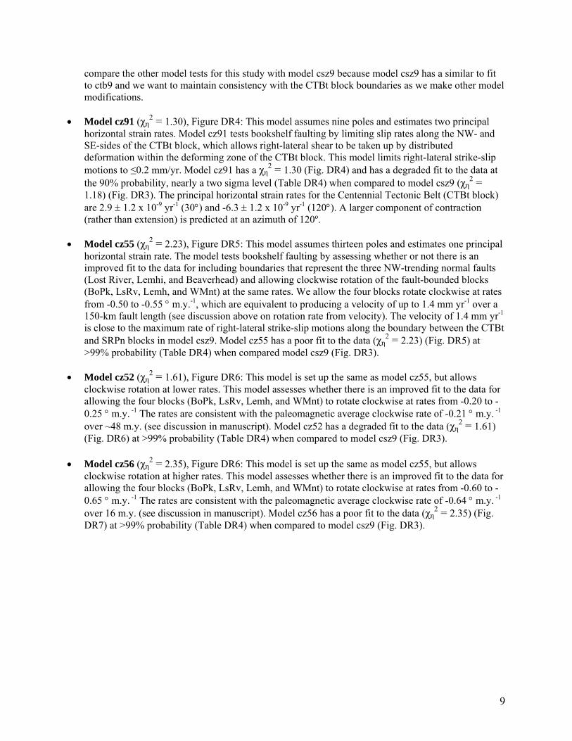
Block Models We present the block models used in the inversions with TDEFNODE (McCaffrey, 2009) that fit the GPS and earthquake data. We follow the approach of Payne et al. (2012) who modified their preferred model ctb9 to test hypotheses related to dike opening rates and post seismic effects of earthquakes. We use the fault configuration of preferred model ctb9 from Payne et al. (2012) and modify it to add faults, constrain slip along block boundaries, or allow rotation of some blocks to test the hypotheses discussed in the manuscript. We use F-distribution tests to evaluate the statistical significance of changes between two models. Table DR4 lists results of F-distribution tests using χη
2 and degrees of freedom (DOF) between model pairs. The F-distributions give the probability that the first model is different from second or that the first model has a better fit to the data than the second model. We apply the maximum confidence level of ≥99% to indicate one model with added boundaries has a better fit to the data over a second model (Stein and Gordon, 1984). Model Descriptions For these tests, the NoAm block is defined by the Stable North American Reference Frame (SNARF) and is the reference frame. Below, we provide additional details of the models used in the inversions, the purpose of the test, and results compared to other models. Model ctb9 (χη
2 = 1.21), Figure DR2: This model tests whether or not shear results from different strain rates in the Snake River Plain and adjacent Centennial Tectonic Belt. Payne et al. (2012) determined this model through a series of inversions where boundaries were added to divide tectonic provinces and F-distribution tests were used to determine statistically significant differences between models pairs. Figure DR2 shows model ctb9 has seven separate poles of rotation for eastern Washington (EWas), eastern Oregon (EOre), Idaho-Wyoming border (IdWy), Great Basin (GrBn), Centennial Tectonic Belt (as combined blocks CTBt/SwMT/EMnt/IBat; labeled as P025 in Fig. DR2), and Snake River Plain – Owyhee-Oregon Plateau (ESRP/CSRP/WSRP/Owhy; labeled as P029). The model also estimates principal horizontal strain rates for the Centennial Tectonic Belt and Great Basin. The principal horizontal strain rates for the Centennial Tectonic Belt are 5.7 0.6 x 10⁻⁹ yr-1 (at an azimuth of 57) and –2.2 0.7 x 10⁻⁹ yr-1 (147). Payne et al. (2012) found that separating the Centennial Tectonic Belt into individual blocks such as IBat and CTBt/SwMT/EMnt resulted in a similar fit to the data (see model ctb7 in Payne et al. 2012).
Model csz9 (χη
2 = 1.18), Figure DR3: This model tests whether or not shear results from different strain rates in the Snake River Plain and adjacent Centennial Tectonic Belt. The model assumes nine poles and estimates three principal horizontal strain rates. The model includes the same boundaries to separate tectonic provinces as model ctb9 (see description above) with the exception of separating the Centennial Tectonic Belt into smaller blocks so that modifications can be made to test “bookshelf faulting” models. The SwMT block with three velocities has the same pole of rotation as the EWas block. We estimate strain rates for the Centennial Tectonic Belt (CTBt), Snake River Plain (SRPn), and Great Basin (GrBn). The χη
2 = 1.18 for model csz9 (Fig. DR3) has a similar fit to the data as model ctb9 since the F-test results in 66% probability (Table DR4), which is less than the 99%. This means the models have the same fit to the data for either one combined block CTBt/SwMT/EMnt/IBat as in model ctb9 or for separate blocks (CTBt, EMnt, and IBat) or when boundaries are added. Additionally, the estimated strain rates and predicted slip vectors are also similar. The Centennial Tectonic Belt has an extensional strain rate of 6.6 0.9 x 10⁻⁹ yr-1 (59), which is similar to the estimate for ctb9. The slip rate vectors between the CTBt and SRPn blocks are 0.3 to 1.5 mm yr-1 for model csz9 compared to 0.3 to 1.4 mm yr-1 for model ctb9. We also estimated a strain rate of -0.1 1.1 x 10⁻⁹ yr-1 (149) for the SRPn block, which is not discernable from zero. We
9
compare the other model tests for this study with model csz9 because model csz9 has a similar to fit to ctb9 and we want to maintain consistency with the CTBt block boundaries as we make other model modifications.
Model cz91 (χη
2 = 1.30), Figure DR4: This model assumes nine poles and estimates two principal horizontal strain rates. Model cz91 tests bookshelf faulting by limiting slip rates along the NW- and SE-sides of the CTBt block, which allows right-lateral shear to be taken up by distributed deformation within the deforming zone of the CTBt block. This model limits right-lateral strike-slip motions to ≤0.2 mm/yr. Model cz91 has a χη
2 = 1.30 (Fig. DR4) and has a degraded fit to the data at the 90% probability, nearly a two sigma level (Table DR4) when compared to model csz9 (χη
2 = 1.18) (Fig. DR3). The principal horizontal strain rates for the Centennial Tectonic Belt (CTBt block) are 2.9 1.2 x 10⁻⁹ yr-1 (30) and -6.3 1.2 x 10⁻⁹ yr-1 (120). A larger component of contraction (rather than extension) is predicted at an azimuth of 120º.
Model cz55 (χη
2 = 2.23), Figure DR5: This model assumes thirteen poles and estimates one principal horizontal strain rate. The model tests bookshelf faulting by assessing whether or not there is an improved fit to the data for including boundaries that represent the three NW-trending normal faults (Lost River, Lemhi, and Beaverhead) and allowing clockwise rotation of the fault-bounded blocks (BoPk, LsRv, Lemh, and WMnt) at the same rates. We allow the four blocks rotate clockwise at rates from -0.50 to -0.55 m.y.-1, which are equivalent to producing a velocity of up to 1.4 mm yr-1 over a 150-km fault length (see discussion above on rotation rate from velocity). The velocity of 1.4 mm yr-1 is close to the maximum rate of right-lateral strike-slip motions along the boundary between the CTBt and SRPn blocks in model csz9. Model cz55 has a poor fit to the data (χη
2 = 2.23) (Fig. DR5) at >99% probability (Table DR4) when compared model csz9 (Fig. DR3).
Model cz52 (χη
2 = 1.61), Figure DR6: This model is set up the same as model cz55, but allows clockwise rotation at lower rates. This model assesses whether there is an improved fit to the data for allowing the four blocks (BoPk, LsRv, Lemh, and WMnt) to rotate clockwise at rates from -0.20 to -0.25 m.y. -1 The rates are consistent with the paleomagnetic average clockwise rate of -0.21 m.y. -1 over ~48 m.y. (see discussion in manuscript). Model cz52 has a degraded fit to the data (χη
2 = 1.61) (Fig. DR6) at >99% probability (Table DR4) when compared to model csz9 (Fig. DR3).
Model cz56 (χη
2 = 2.35), Figure DR6: This model is set up the same as model cz55, but allows clockwise rotation at higher rates. This model assesses whether there is an improved fit to the data for allowing the four blocks (BoPk, LsRv, Lemh, and WMnt) to rotate clockwise at rates from -0.60 to -0.65 m.y. -1 The rates are consistent with the paleomagnetic average clockwise rate of -0.64 m.y. -1 over 16 m.y. (see discussion in manuscript). Model cz56 has a poor fit to the data (χη
2 = 2.35) (Fig. DR7) at >99% probability (Table DR4) when compared to model csz9 (Fig. DR3).
10
Table DR4. Results of F-distribution tests for model pairs. Model χη
2 DOF P (%) csz9 1.18 514 ctb9 1.21 522
66
csz9 1.18 514 cz91 1.30 520
90
csz9 1.18 514 cz55 2.23 521
100
csz9 1.18 514 cz52 1.61 521
100
csz9 1.18 514 cz56 2.35 521
100
χη2 – Reduced chi-square; DOF – Degrees of freedom; P
– Probability that misfit variances are from different distributions.
11
Plots of Model Results Results are shown in Figures DR2 to DR7 with the following:
Pole of rotation (brown dot with 70% confidence ellipse) for poles located within the map region Name of a pole (brown letters, e.g. SRPn for an individual block; P025 or EWas/SwMT for two
blocks with the same pole) Residual velocities (gray vectors with 70% confidence ellipses) shown for misfits between
observed and predicted velocities Principal horizontal strain rate directions (pink arrows) and strain rates (pink letters) Block model configuration with showing only the fault (solid green lines) used in the inversions Model name (e.g. csz9) and inversion results listed as C2/NP/DF, which corresponds to reduced
chi-square (CD), number of free parameters (NP), and degrees of freedom (DF) Name (red letters) of the block (e.g., EWas/SwMT or P025 indicate that multiple blocks have the
same pole of rotation and are noted in the figure caption) Reduced chi-squared of GPS velocities (red numbers) in each block or for all blocks with the
same pole of rotation.
12
Figure DR2. Model ctb9 assumes seven poles and estimates two principal horizontal strain rates. Pole P025 is for multiple blocks CTBt/SwMT/EMnt/IBat, P029 for blocks ESRP/CSRP/WSRP/Owhy, and all others are individual blocks as labeled (Payne et al. 2012; see their Supporting Information).
13
Figure DR3. Model csz9 assumes nine poles and estimates three principal horizontal strain rates. Combined blocks EWas/SwMT have the same pole of rotation and all other blocks are individual poles as labeled.
14
Figure DR4. Model cz91 model assumes nine poles and estimates two principal horizontal strain rates. Combined blocks EWas/SwMT have the same pole of rotation and all other blocks are individual poles as labeled. Model cz91 limits right-lateral strike-slip motions along the northwest and southeast boundaries of the CTBt block and allows faults within the CTBt block to take up distributed deformation.
15
Figure DR5. Model cz55 assumes thirteen poles and estimates one principal horizontal strain rate. Combined blocks EWas/SwMT have the same pole of rotation and all other blocks are individual poles as labeled. This model includes boundaries that represent three NW-trending normal faults (Lost River, Lemhi, and Beaverhead) and allows clockwise rotation of the BoPk, LsRv, Lemh, and WMnt blocks at the same rates from -0.50 to -0.55 ° m.y.-1, which tests if bookshelf faulting occurs in the Centennial Tectonic Belt.
16
Figure DR6. Model cz52 assumes thirteen poles and estimates one principal horizontal strain rate. Combined blocks EWas/SwMT have the same pole of rotation and all other blocks are individual poles as labeled. This model includes boundaries that represent three NW-trending normal faults (Lost River, Lemhi, and Beaverhead) and allows clockwise rotation of the BoPk, LsRv, Lemh, and WMnt blocks at the same rates from -0.20 to -0.25 ° m.y.-1 The model tests if bookshelf faulting occurs over the Centennial Tectonic Belt for lower clockwise rotation rates consistent with long-term, paleomagnetic average rate of -0.21 ° m.y.-1 over ~48 m.y.
17
Figure DR7. Model cz56 assumes thirteen poles and estimates one principal horizontal strain rate. Combined blocks EWas/SwMT have the same pole of rotation and all other blocks are individual poles as labeled. This model includes boundaries that represent three NW-trending normal faults (Lost River, Lemhi, and Beaverhead) and allows clockwise rotation of the BoPk, LsRv, Lemh, and WMnt blocks at the same rates from -0.60 to -0.65 ° m.y.-1 The model tests if bookshelf faulting occurs over the Centennial Tectonic Belt for higher clockwise rotation rates consistent with the paleomagnetic average rate of -0.64 ° m.y.-1 over 16 m.y.
18
Snake River Plain Frame of Reference
We rotate the observed velocities into the “Snake River Plain” frame of reference using the angular velocity for the SRPn block (Snake River Plain and Owyhee-Oregon Plateau) estimated in model csz9 (without calculating the strain rate). In Cartesian coordinates, the pole is ωx = 0.0865; ωy = 0.1771, ωz = -0.2173. Figure DR8 shows the 1994–2010 velocity field in the “Snake River Plain” frame of reference. It also shows the Centennial Tectonic Belt and Intermountain Seismic Belt are extending and moving to the northeast relative to the Snake River Plain. Eastern Oregon and southeastern Washington (regions west of the Idaho batholith) are generally moving to the east.
19
Figure DR8. Map showing horizontal velocities rotated into a “Snake River Plain” frame of reference using the angular velocity of the SRPn block (Snake River Plain and Owyhee-Oregon Plateau) from model csz9. Velocities are shown by blue arrows and 70% confidence ellipses.
20
Gravitational Potential Energy (GPE) Calculations
We calculate the GPE (in units of N/m) for the grid points shown in Figures DR-9 through DR-12. We use the ETOPO5 topographic data set to assign elevations at a longitude (X) and latitude (Y) spacing of 0.2°, which are shown in Figure DR-9. The GPE are calculated using the elevations (Fig. DR-9) and density models listed in Table 3 of the manuscript. Figures DR-10A, 11A, and 12A show the GPE values for the three sets of density models referred to as “Underplated Only”, Sill Only”, and “Original”, respectively (see manuscript text for discussion of models). To evaluate longer wavelength features, the GPE values were smoothed using a 3 x 3 moving-window low-pass filter with the weights listed in Table DR-5. Figures DR-10B, 11B, and 12B show the smoothed GPE (in units of N/m). The GPE gradients (in units of N/m/m) shown in manuscript in Figures 4A, 4B and 4C were calculated in X and Y directions using the smoothed GPE values divided by the grid-spacing distances (~16 km in the X and ~22 km in the Y directions). For the X direction, the east longitude GPE value was subtracted from the west longitude GPE value and for the Y direction south latitude GPE value was subtracted from the north latitude GPE value. Table DR-5. Weights of the 3 x 3 smoothing window.
1/15 2/15 1/15
2/15 3/15 2/15
1/15 2/15 1/15
21
Figure DR9. Map showing the elevations (meters) used in the GPE calculations at a 0.2° longitude (X) and latitude (Y) spacing obtained from the ETOPO5 topographic data set. Gold lines show boundaries for the density models.
22
Figure DR10. Maps show (A) GPE and (B) smoothed GPE values (1013 N m-1) for “Underplated Only” density models (gold boundaries).
23
Figure DR11. Maps show (A) GPE and (B) smoothed GPE values (1013 N m-1) for “Sill Only” density models (gold boundaries).
24
Figure DR12. Maps show (A) GPE and (B) smoothed GPE values (1013 N m-1) for “Original” density models (gold boundaries).
25
References Advanced National Seismic System, 2011, ANSS catalog search: http://www.ncedc.org/anss/catalog-
search.html (January 2011).
Bock et al., 1997. Southern California Permanent GPS Geodetic Array: Continuous measurements of crustal deformation between the 1992 Landers and 1994 Northridge earthquakes: Journal of Geophysical Research, v. 102, p. 18,013-18,033.
Centroid-Moment-Tensor Project, 2009, Global CMT Catalog Search: http://www.globalcmt.org/CMTsearch.html/ (April 2011).
Doser, D.I. and Smith, R.B., 1989, An assessment of source parameters of earthquakes in the Cordillera of the western United States: Bulletin of the Seismological Society of America, v. 77, p. 1383-1409.
Dow, J.M, Neilan, R.E. and Rizos, C., 2009. The International GNSS Service in a changing landscape of Global Navigation Satellite Systems: Journal of Geodesy, v. 83, p. 191-198.
Jackson, S.M. and Zollweg, J.E., 1988, Seismic studies of an earthquake sequence in the White Cloud Peaks, Idaho: Seismological Research Letters, v. 59, p. 6.
Herrmann, R. B., Benz, H., and Ammon, C. J., 2011, Monitoring the earthquake source process in North America: Bulletin of the Seismological Society of America, v. 101, p. 2609-2625, doi:10.1785/0120110095.
McCaffrey, R., 2009, Time-dependent inversion of three-component continuous GPS for steady and transient sources in northern Cascadia: Geophysical Research Letters, v. 36, L07304, doi:10.1029/2008GL036784.
McCaffrey, R., Qamar, A.I., King, R.W., Wells, R., Khazaradze, G., Williams, C.A., Stevens, C.W., Vollick, J.J. and Zwick, P.C., 2007. Fault locking, block rotation and crustal deformation in the Pacific Northwest: Geophysical Journal International, v. 169, p. 1315-1340.
Payne, S.J., McCaffrey, R. and King, R.W., 2008, Strain rates and contemporary deformation in the Snake River Plain and surrounding Basin and Range from GPS and seismicity: Geology, v. 36, p. 647-650.
Payne, S.J., McCaffrey, R. and King, R.W. and Kattenhorn, S.A., 2012, An new interpretation of deformation rates in the Snake River Plain and adjacent Basin and Range regions from GPS measurements: Geophysical Journal International, v. 189, p. 101-122.
Pezzopane, S.K. and Weldon, R. J., 1993, Tectonic role of active faulting in central Oregon: Tectonics, v. 12, p. 1140-1169.
Richins, W.D., Pechmann, J.C., Smith, R.B., Langer, C.J., Goter, S.K., Zollweg, J.E. and King, J.J., 1987, The 1983 Borah Peak, Idaho earthquake and its aftershocks: Bulletin of the Seismological Society of America, v. 77, p. 694-723.
St. Louis Univeristy Earthquake Center, 2011, St. Louis University Digital Data Focal Mechanism Page: http://www.eas.slu.edu/eqc/eqc_mt/MECH.NA/index.html (January 2011).
Stein, S. and Gordon, R.G., 1984. Statistical tests of additional plate boundaries from plate motion inversions: Earth and Planetary Science Letters, v. 69, p. 401-412.
Stickney, M.C., 1997, Seismic source zones in southwestern Montana: Montana Bureau of Mines and Geology Open-File Report 366, 52 p.
26
Stickney, M.C., 2007. Historic earthquakes and seismicity in southwestern Montana: Northwest Geology, v. 36, p. 167-186.
U.S. Geological Survey, 2007, Quaternary Fault and Fold Database for the United States: http://earthquake.usgs.gov/regional/qfaults/ (accessed 17 April 2007).
Zollweg, J.E. and Richins, W.D., 1985, Later aftershocks of the 1983 Borah Peak, Idaho earthquake and related activity in central Idaho, in Proc. Workshop XXVIII on the 1983 Borah Peak, Idaho, earthquake: U.S. Geological Survey Open-File Report 85-290, p. 345-367.