104
www.retscreen.net International RETScreen ® Clean Energy Decision Support Centre RETScreen ® Software Online User Manual Ground-Source Heat Pump Project Model
| Date post: | 06-Apr-2018 |
| Category: |
Documents |
| Upload: | maria-mikela-chatzimichailidou |
| View: | 217 times |
| Download: | 0 times |

8/3/2019 GSHP3
http://slidepdf.com/reader/full/gshp3 1/104
www.retscreen.net
InternationalRETScreen®
Clean Energy Decision Support Centre
RETScreen®
Software
Online User Manual
Ground-Source Heat PumpProject Model

8/3/2019 GSHP3
http://slidepdf.com/reader/full/gshp3 2/104
Background
This document allows for a printed version of the RETScreen® Software Online User Manual, which is an integral partof the RETScreen Software. The online user manual is a Help file within the software. The user automaticallydownloads the online user manual Help file while downloading the RETScreen Software.
Reproduction
This document may be reproduced in whole or in part in any form for educational or nonprofit uses, without specialpermission, provided acknowledgment of the source is made. Natural Resources Canada would appreciate receivinga copy of any publication that uses this report as a source. However, some of the materials and elements found inthis report are subject to copyrights held by other organizations. In such cases, some restrictions on the reproductionof materials or graphical elements may apply; it may be necessary to seek permission from the author or copyrightholder prior to reproduction. To obtain information concerning copyright ownership and restrictions on reproduction,please contact RETScreen International.
Disclaimer
This report is distributed for informational purposes and does not necessarily reflect the views of the Government ofCanada nor constitute an endorsement of any commercial product or person. Neither Canada nor its ministers,officers, employees or agents makes any warranty in respect to this report or assumes any liability arising out of this
report.
ISBN: 0-662-40450-5
Catalogue no.: M39-118/2005E-PDF
© Minister of Natural Resources Canada 1997-2005.

8/3/2019 GSHP3
http://slidepdf.com/reader/full/gshp3 3/104
RETScreen® Ground-Source Heat Pump Project Model
TABLE OF CONTENTS
Brief Description and Model Flow Chart ................................................................................... 4
Ground-Source Heat Pump Project Model ................................................................................ 9
Energy Model .............................................................................................................................. 10
Heating and Cooling Load Calculation..................................................................................... 23
Cost Analysis ............................................................................................................................... 34
Financial Summary..................................................................................................................... 56
Greenhouse Gas (GHG) Emission Reduction Analysis........................................................... 72
Sensitivity and Risk Analysis ..................................................................................................... 83
Product Data................................................................................................................................ 92
Weather Data .............................................................................................................................. 93
Cost Data...................................................................................................................................... 94
Training and Support ................................................................................................................. 95
Term of Use ................................................................................................................................. 96
Bibliography ................................................................................................................................ 98
Index............................................................................................................................................. 99
GSHP.3

8/3/2019 GSHP3
http://slidepdf.com/reader/full/gshp3 4/104
RETScreen® Software Online User Manual
Brief Description and Model Flow Chart
RETScreen® International is a clean energy awareness, decision-support and capacity buildingtool. The core of the tool consists of a standardised and integrated clean energy project analysissoftware that can be used world-wide to evaluate the energy production, life-cycle costs and
greenhouse gas emission reductions for various types of energy efficient and renewable energytechnologies (RETs). Each RETScreen technology model (e.g. Ground-Source Heat PumpProject, etc.) is developed within an individual Microsoft® Excel spreadsheet "Workbook" file.The Workbook file is in-turn composed of a series of worksheets. These worksheets have acommon look and follow a standard approach for all RETScreen models. In addition to thesoftware, the tool includes: product, weather and cost databases; an online manual; a Website; anengineering textbook, project case studies; and a training course.
Model Flow Chart
Complete each worksheet row by row from top to bottom by entering values in shaded cells. To
move between worksheets simply "click" on the tabs at the bottom of each screen or on the"blue-underlined" hyperlinks built into the worksheets. The RETScreen Model Flow Chart ispresented below.
RETScreen Model Flow Chart
GSHP.4

8/3/2019 GSHP3
http://slidepdf.com/reader/full/gshp3 5/104
RETScreen® Ground-Source Heat Pump Project Model
Data & Help Access
The RETScreen Online User Manual, Product Database and Weather Database can be accessedthrough the Excel menu bar under the "RETScreen" option, as shown in the next figure. The
icons displayed under the RETScreen menu bar are displayed in the floating RETScreen toolbar.Hence the user may also access the online user manual, product database and weather databaseby clicking on the respective icon in the floating RETScreen toolbar. For example, to access theonline user manual the user clicks on the "?" icon.
RETScreen Menu and Toolbar
The RETScreen Online User Manual, or help feature, is "cursor location sensitive" and thereforegives the help information related to the cell where the cursor is located.
Cell Colour Coding
The user enters data into "shaded" worksheet cells. All other cells that do not require input dataare protected to prevent the user from mistakenly deleting a formula or reference cell. TheRETScreen Cell Colour Coding chart for input and output cells is presented below.
RETScreen Cell Colour Coding
GSHP.5

8/3/2019 GSHP3
http://slidepdf.com/reader/full/gshp3 6/104
RETScreen® Software Online User Manual
Currency Options
To perform a RETScreen project analysis, the user may select a currency of their choice from the"Currency" cell in the Cost Analysis worksheet.
The user selects the currency in which the monetary data of the project will be reported. Forexample, if the user selects "$," all monetary related items are expressed in $.
Selecting "User-defined" allows the user to specifythe currency manually by entering a name or symbolin the additional input cell that appears adjacent to thecurrency switch cell. The currency may be expressedusing a maximum of three characters ($US, £, ¥, etc.).To facilitate the presentation of monetary data, thisselection may also be used to reduce the monetarydata by a factor (e.g. $ reduced by a factor of athousand, hence k$ 1,000 instead of $ 1,000,000).
If "None" is selected, all monetary data are expressedwithout units. Hence, where monetary data is usedtogether with other units (e.g. $/kWh) the currencycode is replaced with a hyphen (-/kWh).
The user may also select a country to obtain theInternational Standard Organisation (ISO) three-lettercountry currency code. For example, if Afghanistan isselected from the currency switch drop-down list, allproject monetary data are expressed in AFA. The firsttwo letters of the country currency code refer to the
name of the country (AF for Afghanistan), and thethird letter to the name of the currency (A forAfghani).
For information purposes, the user may want to assigna portion of a project cost item in a second currency,to account for those costs that must be paid for in acurrency other than the currency in which the projectcosts are reported. To assign a cost item in a secondcurrency, the user must select the option "Secondcurrency" from the "Cost references" drop-down list
cell.
Some currency symbols may be unclear on the screen(e.g. €); this is caused by the zoom settings of thesheet. The user can increase the zoom to see thosesymbols correctly. Usually, symbols will be fullyvisible on printing even if not fully appearing on thescreen display. List of Units, Symbols and Prefixes
GSHP.6

8/3/2019 GSHP3
http://slidepdf.com/reader/full/gshp3 7/104
RETScreen® Ground-Source Heat Pump Project Model
Units, Symbols & Prefixes
The previous table presents a list of units, symbols and prefixes that are used in the RETScreenmodel.
Note: 1. The gallon (gal) unit used in RETScreen refers to US gallon and not to imperialgallon.
2. The tonne (t) unit used in RETScreen refers to metric tonnes.
Saving a File
To save a RETScreen Workbook file, standard Excel savingprocedures should be used. The original Excel Workbook filefor each RETScreen model can not be saved under its originaldistribution name. This is done so that the user does not save-over the "master" file. Instead, the user should use the "File,
Save As" option. The user can then save the file on a harddrive, diskette, CD, etc. However, it is recommended to savethe files in the "MyFiles" directory automatically set by theRETScreen installer program on the hard drive.
The download procedure is presented in the following figure.The user may also visit the RETScreen Website atwww.retscreen.net for more information on the downloadprocedure. It is important to note that the user should notchange directory names or the file organisation automaticallyset by RETScreen installer program. Also, the main
RETScreen program file and the other files in the "Program"directory should not be moved. Otherwise, the user may not beable to access the RETScreen Online User Manual or theRETScreen Weather and Product Databases.
RETScreen Download Procedure
GSHP.7

8/3/2019 GSHP3
http://slidepdf.com/reader/full/gshp3 8/104
RETScreen® Software Online User Manual
Printing a File
To print a RETScreen Workbook file, standard Excel printing procedures should be used. Theworkbooks have been formatted for printing the worksheets on standard "letter size" paper with aprint quality of 600 dpi. If the printer being used has a different dpi rating then the user must
change the print quality dpi rating by selecting "File, Page Setup, Page and Print Quality" andthen selecting the proper dpi rating for the printer. Otherwise the user may experience qualityproblems with the printed worksheets.
GSHP.8

8/3/2019 GSHP3
http://slidepdf.com/reader/full/gshp3 9/104
RETScreen® Ground-Source Heat Pump Project Model
Ground-Source Heat Pump Project Model
The RETScreen® International Ground-Source Heat Pump Project Model can be used world-wide
to easily evaluate the energy production (or savings), life-cycle costs and greenhouse gasemissions reduction for the heating and/or cooling of residential, commercial, institutional and
industrial buildings. The model can be used to evaluate both retrofit and new constructionprojects using either ground-coupled (horizontal and vertical closed-loop) or groundwater heatpumps.
Six worksheets ( Energy Model, Equipment Data, Cost Analysis, Greenhouse Gas Emission
Reduction Analysis (GHG Analysis), Financial Summary and Sensitivity and Risk Analysis
(Sensitivity)) are provided in the Ground-Source Heat Pump Project Workbook file.
The Energy Model and Equipment Data worksheets are completed first. The Cost Analysis worksheet should then be completed, followed by the Financial Summary worksheet. The GHG
Analysis and Sensitivity worksheets are optional analyses. The GHG Analysis worksheet isprovided to help the user estimate the greenhouse gas (GHG) mitigation potential of the
proposed project. The Sensitivity worksheet is provided to help the user estimate the sensitivityof important financial indicators in relation to key technical and financial parameters. In general,the user works from top-down for each of the worksheets. This process can be repeated severaltimes in order to help optimise the design of the wind energy project from an energy use and coststandpoint.
In addition to the worksheets that are required to run the model, the Introduction worksheet and Blank Worksheets (3) are included in the Ground-Source Heat Pump Project Workbook file. The Introduction worksheet provides the user with a quick overview of the model. Blank Worksheets
(3) are provided to allow the user to prepare a customised RETScreen project analysis. Forexample, the worksheets can be used to enter more details about the project, to prepare graphs
and to perform a more detailed sensitivity analysis.
As part of the RETScreen Clean Energy Project Analysis Software, the Energy Model and Heating and Cooling Load Calculation worksheets are used to help the user calculate the annualenergy production for a GSHP project based upon local site conditions and systemcharacteristics. Results are calculated in common megawatt-hour (MWh) units for easycomparison of different technologies.
The site conditions associated with estimating the heating and cooling loads and the energydemand of the building where the ground-source heat pump system is to be installed are detailedbelow.
GSHP.9

8/3/2019 GSHP3
http://slidepdf.com/reader/full/gshp3 10/104
RETScreen® Software Online User Manual
Energy Model
As part of the RETScreen Clean Energy Project Analysis Software, the Energy Model andHeating and Cooling Load Calculation worksheets are used to help the user calculate the annualenergy production for a GSHP project based upon local site conditions and system
characteristics. Results are calculated in common megawatt-hour (MWh) units for easycomparison of different technologies.
Site Conditions
The site conditions associated with estimating the annual energy production of a ground-sourceheat pump project are detailed below.
Project name
The user-defined project name is given for reference purposes only.
For more information on how to use the RETScreen Online User Manual, Product Database andWeather Database, see Data & Help Access.
Project location
The user-defined project location is given for reference purposes only.
Available land area
The user enters the available land area (m²) at the proposed site. This land area is compared to
the "Typical land area required" calculated in the model. A warning message will be displayed inthe model if the selected system is not likely to fit in the available land area. The user shouldthen adjust the system design (i.e. vertical vs. horizontal ground heat exchangers, layout, etc.).See "Typical land area required" description which follows.
Soil type
The user selects the type of soil that is found at the proposed site. The soil type has a largeinfluence on the size of the ground heat exchanger (GHX). For example, a light dry soil willrequire a much longer horizontal GHX than a heavy damp soil would. This is due to the poorerheat transfer characteristics and the lower density of the lighter and dryer soil. The following
table presents the properties of the eight soil types considered in the GSHP model [ASHRAE,1995]. An easy finger assessment procedure for determining soil types is available in theliterature [McRae, 1988].
GSHP.10

8/3/2019 GSHP3
http://slidepdf.com/reader/full/gshp3 11/104
RETScreen® Ground-Source Heat Pump Project Model
Soil Type ConductivityW/(m·°C)
Diffusivitym
2 /s
Densitykg/m
3Heat Capacity
kJ/(kg·°C)
Light Soil – Damp(Loose sand, silt)
0.9 5.16e-7 1,600 1.05
Light Soil – Dry(Loose sand, silt)
0.3 2.84e-7 1,400 0.84
Heavy Soil – Damp(Clay, compacted sand, loam)
1.3 6.45e-7 2,100 0.96
Heavy Soil – Dry(Clay, compacted sand, loam)
0.9 5.16e-7 2,000 0.84
Light Rock (Limestone)
2.4 1.03e-6 2,800 0.84
Heavy Rock (Granite)
3.5 1.29e-6 3,200 0.84
Permafrost – Light 1.4 1.10e-6 1,580 0.76Permafrost – Dense 2.0 1.37e-6 2,070 0.69
Soil Types Defined in the GSHP Model
Design heating load
The building design heating load (kW) is calculated in the Heating and Cooling Load worksheetand copied automatically to the Energy Model worksheet.
Note: At this point, the user should complete the Heating and Cooling Load worksheet.
Design cooling load
The building design cooling load (kW) is calculated in the Heating and Cooling Load worksheetand copied automatically to the Energy Model worksheet.
System Characteristics
The system characteristics associated with estimating the annual energy production of a ground-source heat pump system and establishing a comparison with a base case system are detailedbelow. The system characteristics are divided into four sub-sections: Base Case HVAC System,Ground Heat Exchanger System, Heat Pump System and Supplemental Heating and HeatRejection System.
Base Case HVAC System
This sub-section allows the user to define the seasonal performances of the conventional heating,ventilation and air conditioning (HVAC) system that would be displaced by the GSHP system.
Building has air-conditioning?
The user indicates by selecting from the drop-down list whether or not an air-conditioningsystem is used in the building. The selection made in this box alters the calculation algorithm toinclude or exclude the energy savings or losses that occur due to changes in cooling load. If thebuilding is not equipped with air-conditioning, no reduction in cooling load is calculated andhence, no savings are realised. If an air-conditioning system is included, the effects of the
GSHP.11

8/3/2019 GSHP3
http://slidepdf.com/reader/full/gshp3 12/104
RETScreen® Software Online User Manual
ground-source heat pump system on summer cooling energy demands are taken intoconsideration.
Changing the selection in this field affects the worksheet display in several locations. Indicatingthat an air-conditioning system is used causes certain input fields to be added because someadditional information is required. Selecting no air-conditioning removes the extraneous entry
fields.
Heating fuel type
The user selects the type of fuel that is used to heat the building. A list of common fuels isprovided in the drop-down list. This selection allows the model to estimate the peak electricalload that would be required by the conventional heating system. If the user selects "Other," themodel assumes that the fuel type has no impact on the base case electric demand. The tablebelow provides the heats of combustion for the heating energy avoided.
Fuel Heating Value
Note: Propane is expressed in terms of liquefied propane.
Heating system seasonal efficiency
The user enters the annual heating system efficiency (%) (not the instantaneous or peak efficiency). This value should include the effects of cycling and part load performance as well asany loss of heat because of ducting that runs outside of the building envelope. This value is usedto estimate the gross energy/fuel requirement to meet the building's heating demand in the basecase scenario.
Typical values of heating system seasonal efficiency are tabulated in the table below. Thesevalues should be reduced by 10% if ducting runs outside of the insulated envelope (e.g. in attics).
Typical Heating Systems Seasonal Efficiencies
GSHP.12

8/3/2019 GSHP3
http://slidepdf.com/reader/full/gshp3 13/104
RETScreen® Ground-Source Heat Pump Project Model
Air-conditioner seasonal COP
The seasonal Coefficient Of Performance (COP) is a property of the air-conditioning device andrepresents the average expected performance over the cooling season expressed in terms of thecooling energy output of the device divided by the energy input to the device. This value is used
to estimate the net electrical energy requirement and peak load to meet the building's coolingenergy demand for the base case HVAC system.
Typical values of COP are tabulated in the table below. These values should be reduced by 10%if ducting runs outside of the insulated envelope (e.g. in attics).
Cooling System Type Typical Annual COP
Window air-conditioner 2.4Standard DX (direct expansion)
air-conditioner and air-source heat pumps3.0
High-efficiency air-conditioner 3.5High-efficiency commercial chiller 5.0
Ground-source heat pump 4.4 Typical Annual COP for Air-Conditioning Systems
Ground Heat Exchanger System
This sub-section allows the user to define the type of GSHP system that will be evaluated.
System type
The user selects the system type. The options from the drop-down list are: "Vertical closed-loop," "Horizontal closed-loop" and "Groundwater." The vertical closed-loop system is based on
one U-tube per borehole type ground heat exchanger, while the horizontal system is based on astack two-pipe arrangement as shown in the next figure.
The primary type of groundwater system considered is the supply and injection well system,although standing column systems can also be evaluated by the model if the cost of well drillingis corrected to compensate the absence of a separate injection well.
1.8 m1.2 m
Horizontal Heat Exchanger Configuration
Selecting "Horizontal closed-loop" will lead to the largest required land area but will result inlower initial costs than vertical closed-loop systems. Groundwater systems usually require thesmallest land area and can offer the highest performances. However, availability of groundwaterand environmental regulations can sometimes prohibit the use of this type of system.
GSHP.13

8/3/2019 GSHP3
http://slidepdf.com/reader/full/gshp3 14/104
RETScreen® Software Online User Manual
Design criteria
The user selects the design criteria from the two options in the drop-down list: "Heating" and"Cooling." This selection is used in the model to evaluate the size of the ground heat exchanger,the required groundwater flow, and to size the heat pumps.
This selection will have a large influence on the size of the ground heat exchanger, as well as theheat pump and supplemental heating and cooling equipment. For example, many buildings inmoderate to warm climates, and to a lesser extent in colder climates, have cooling loads thattypically dominate heating loads. Selecting a ground heat exchanger to entirely meet the coolingload could lead to an excessively large ground heat exchanger that could make a GSHP systemfinancially unviable. In such a situation it is often advisable to size the ground heat exchanger tomeet only the heating load and have a supplemental heat rejector (e.g. a cooling tower) tocompensate for the excess cooling demand. In cold climates this situation can be reversed andsizing the ground heat exchanger for cooling loads can result in a smaller ground heat exchangerbut will require the use of supplemental heat in the winter.
The choice of designing the system based on cooling or heating load will be closely linked to thecost and financial viability of each project and can be evaluated by the user during the pre-feasibility stage through sensitivity analysis.
Typical land area required
The model calculates the typical land area (m²) required for the selected GSHP system type. Thisland area is compared to the available land area entered by the user; if the available land area isless than the typical land area required, a "Insufficient land area" warning message in redcharacters will appear next to this value. If this warning message appears, the user can changethe GHX system type or layout to fit the available land area.
The typical land area required for a groundwater system is based on a 6 m radius per well andincludes the presence of injection wells. The typical land area for a vertical closed-loop system isbased on an average borehole depth of 91 m.
Typical values for land area range from 50 to 95 m²/kW for horizontal systems and 1.5 to12 m²/kW for vertical systems.
Ground heat exchanger layout
The user selects one of three layout options: "Standard," "Compact" and "Very compact." Thisselection determines the minimum separation between boreholes in a vertical system andbetween trenches in a horizontal system. The table presents the typical distances used in themodel corresponding to each layout.
Type of GHXLayout
Borehole Separationm
Trench Separationm
Standard 6.1 3.7Compact 3.7 2.4
Very compact 2.4 1.5 Distances between Boreholes and Trenches
GSHP.14

8/3/2019 GSHP3
http://slidepdf.com/reader/full/gshp3 15/104
RETScreen® Ground-Source Heat Pump Project Model
While a smaller separation distance will reduce the typical land area required it would increasethe total length of ground heat exchanger required. Moreover, long term heat imbalance on theground heat exchanger (cooling loads much greater than heating loads or vice-versa) will reduceto a greater extent the efficiency of closely packed GHXs. When a large difference existsbetween the heating and cooling loads, long term effects on non-standard layouts should be
thoroughly investigated.
Total borehole length
The model calculates the cumulative borehole length (m) needed to meet the building heating orcooling load depending on the selected design option. The borehole length depends on manyfactors such as the earth temperature, soil type, building load and energy demand. This value isused to obtain the typical land area based on an average depth of 91 m per individual borehole.
Typical values for cumulative borehole length are between 10 to 25 m/kW.
Total loop length
The model calculates the total loop length (m) needed to meet the building heating or coolingload depending on the selected design option. The loop length depends on many factors such asthe earth temperature, soil type, building load and energy demand, trench separation(ground heatexchanger layout). This value represents the approximate length of pipe that would be installedunderground.
Typical values for total loop length for a stack two-pipe system are between 40 to 65 m/kW.
Total trench length
This value is simply half the total loop length since the horizontal system considered is a two-pipe system. This value is used along with the separation distance to obtain the typical land arearequired.
Typical values for total loop length for a stack two-pipe system are between 20 to 33 m/kW.
Pumping depth
The user enters the depth (m) from which the water will be pumped. This value is used toevaluate the pumping power required. The pumping depth corresponds to the distance to thestatic water level in the well to which is added the drawdown. This drawdown corresponds to a
lowering of the static water level in the well required to insure the pumping rate. In addition tothe pumping depth, a supplementary 15 m of head is added to the pumping head to account forinjection well pressure and pressure losses in the piping.
Typical values for pumping depth can vary significantly according to location, with values in the30 to 60 m range being common. Excessive pumping depth will significantly increase thepumping power and reduce the GSHP system's COP, and consequently impact the cost of theproject.
GSHP.15

8/3/2019 GSHP3
http://slidepdf.com/reader/full/gshp3 16/104
RETScreen® Software Online User Manual
Wellbore depth
The user enters the wellbore depth (m) for a typical well at the site. This value is used to evaluatethe cost of drilling the wells.
Typical values for wellbore depth range from 50 to 250 m for open loop systems but can be asdeep as 500 m for standing column wells.
Maximum well flow rate
The user enters the maximum flow rate (L/s) that can be delivered on a continuous basis by atypical well. This information usually comes from test wells but initial estimates can sometimesbe obtained from experienced well drillers or hydro-geologists at the site. This value is used todetermine the number of wells required to meet the building energy demand for both cooling andheating.
Typical values for maximum flow rate vary from 0.5 L/s to over 60 L/s.
Required groundwater flow rate
The model calculates the total groundwater flow rate (L/s) needed to meet the building designheating and cooling load. The flow rate depends on the groundwater temperature and thebuilding's loop heat exchanger efficiency. To determine the required flow rate, the modelassumes a 2.8°C approach temperature at the heat exchanger, between the groundwater loop andthe building loop.
Typical values for "Required groundwater flow rate" are usually 0.05 L/s/kW or less.
Number of supply wells requiredBased on the required groundwater flow rate and the maximum well flow rate, the modelcalculates the total number of supply wells required. The same number of injection wells isassumed.
Heat Pump System
This sub-section allows the user to define the average efficiency of the heat pumps used in theGSHP system.
Average heat pump efficiencyThe user selects the average heat pump efficiency from the options in the drop-down list:"Standard," "Medium," "High" and "User-defined." Values for heating and cooling COP's aredisplayed in the spreadsheet in the cells below.
Standard, medium and high efficiencies are steady state COPs and not seasonal values. Theseefficiencies are determined under standard test conditions as defined by the Canadian Standards
GSHP.16

8/3/2019 GSHP3
http://slidepdf.com/reader/full/gshp3 17/104
RETScreen® Ground-Source Heat Pump Project Model
Association (CSA) Standard 446 or the Air-conditioning and Refrigeration Institute (ARI)standards 325 and 330. Both organisations have directories which list heat pumps certified undertheir specific standards. The table below shows the COPs corresponding to the three levels of performance along with the standard test conditions.
(1: EWT = Entering Water Temperature - water going into the heat pump;2: GWHP = Groundwater heat pump; 3 = GCHP = Ground-coupled heat pump)
Heat Pump COP and Standard Test Conditions
When the user selects "User-defined" a product selection can be made from the online product
database to obtain the heating and cooling COP values. These data can be pasted from thedialogue box to the spreadsheet by clicking on the "Paste Data" button.
Since GSHP systems are generally made up of a number of small to medium size heat pumps,the COP value represents the weighted average of all machines in the system. Selecting a higherefficiency level will reduce electrical consumption but increase the initial cost of the heat pumps.In some cases the GHX might also be somewhat larger for more efficient heat pumps, since themotor energy saved by the efficient heat pump has to be made up through the GHX in heatingmode. Cooling GHX length using higher efficiency heat pumps will however be shorter.
Heat pump manufacturer
The user enters the name of the heat pump manufacturer. This information is given for referencepurposes only. The user can consult the RETScreen Online Product Database for moreinformation.
Heat pump model
The user enters the name of the heat pump model. This information is given for referencepurposes only. The user can consult the RETScreen Online Product Database for moreinformation.
Standard cooling COP
See Average heat pump efficiency explanation.
Standard heating COP
See Average heat pump efficiency explanation.
GSHP.17
8/3/2019 GSHP3
http://slidepdf.com/reader/full/gshp3 18/104
RETScreen® Software Online User Manual
Total standard heating capacity
The model calculates the suggested total standard heating capacity (kW) of the heat pumps. Thisvalue is obtained through the building design heating load or the building design cooling load,and is corrected for the difference between standard rating conditions and actual building's
design conditions. The heating capacity is calculated for the building's block load. In a typicaldistributed heat pump system, the actual size of each zone's heat pump will be selected on thatzone's peak load. Therefore, the summation of all installed heat pump heating or coolingcapacities will usually exceed the standard cooling capacity calculated by the model.
Units switch: The user can choose to express the total standard heating capacity in differentunits by selecting among the proposed set of units: "MW," "million Btu/h," "boiler hp,""ton (cooling)," "hp," "W." This value is for reference purposes only and is not required to runthe model.
The value for total standard heating capacity depends on the "Design criteria" option chosen bythe user.
Heating load design criteria: When the user selects "Heating" as the design criteria, the GHX issized to meet the heating load while the heat pump system is sized to meet the maximum valuebetween cooling or heating load under standard rating conditions. This selection assumes thatwhen a GSHP system is installed, the cooling load must, at a minimum, be met by the installedheat pumps so that no other mechanical cooling equipment, other than supplemental heatrejection to compensate for undersize GHX, is required. If the building's heating requirementsare higher than the cooling requirements, the heat pumps will be sized according to the building'sheating energy demand. This may lead to standard cooling capacity far in excess of the actualbuilding's requirements. If the heat pump system cooling capacity exceeds 150% of the buildingenergy demand, the "Oversized" warning message in red characters appears beside the value for
"Total standard cooling capacity." It is generally recommended not to design a GSHP systemwith cooling capacities that are far in excess of the actual building's energy demand. Oversizingthe cooling equipment usually leads to control problems and unacceptable performances,especially with regard to dehumidification. Systems with advanced control options, such asvariable speed compressors, can eliminate this constraint.
Cooling load design criteria: When the user selects "Cooling" as the design criteria, the GHX issized to meet the cooling load AND the heat pumps are also sized to meet the entire coolingdemand. If the building's cooling load is higher than the heating load, this will lead to a heatpump system with standard capacity higher than the building's required heating capacity.However, if the cooling load is lower than the heating load, the standard heat pump systemheating capacity might not be sufficient to meet the building's heating demand. In such cases,
supplemental heating would be required. Designing the heat pumps and the GHX for coolingloads can also lead to standard heat pump system capacities, in heating mode, that are in excessof what the GHX can deliver. In such cases the "Insufficient GHX size" warning messageappears in red characters beside the value for "Total standard heating capacity." In this situation,the model assumes that the heat pumps will be able to deliver only a fraction of their standardcapacity and will require supplemental heat even though the heat pump system might havesufficient capacity to meet the building's demand.
GSHP.18

8/3/2019 GSHP3
http://slidepdf.com/reader/full/gshp3 19/104
RETScreen® Ground-Source Heat Pump Project Model
Total standard cooling capacity
The model calculates the suggested total standard cooling capacity (kW) of the heat pumps. Thisvalue is obtained through the building's design cooling load and is corrected for the differencebetween standard rating conditions and actual building's design conditions. The cooling capacity
is calculated for the building's block load. In a typical distributed heat pump system, the actualsize of each zone's heat pump will be selected on that zone's peak load. Therefore, thesummation of all installed heat pump cooling capacities will usually exceed the standard coolingcapacity calculated by the model.
Units switch: The user can choose to express the total standard cooling capacity in differentunits by selecting among the proposed set of units: "MW," "million Btu/h," "boiler hp,""ton (cooling)," "hp," "W." This value is for reference purposes only and is not required to runthe model.
The value for total standard cooling capacity depends on the "Design criteria" option chosen bythe user.
Heating load design criteria: When the user selects "Heating" as the design criteria the heat pumpsystem is sized to meet the maximum value between cooling or heating load under standardrating conditions. This selection assumes that when a GSHP system is installed, the cooling loadmust, at a minimum, be met by the installed heat pumps so that no other mechanical coolingequipment, other than supplemental heat rejection to compensate for undersized GHX, isrequired. If the building's heating requirement is higher than the cooling requirement, the heatpumps will be sized according to the building's heating demand. This may lead to standardcooling capacity far in excess of the actual building's requirements. If the heat pump systemcooling capacity exceeds 150% of the building demand, the "Oversized" warning message in redcharacters appears beside the value for "Total standard cooling capacity." It is generally
recommended not to design a GSHP system with cooling capacities that are far in excess of theactual building's demand. Oversizing the cooling equipment usually leads to control problemsand unacceptable performances, especially with regard to dehumidification. Systems withadvanced control options, such as variable speed compressors, can eliminate this constraint.
Cooling load design criteria: When the user selects "Cooling" as his design criteria the heatpumps are always sized to meet the entire cooling load.
Supplemental Heating and Heat Rejection System
This sub-section presents the characteristics of the supplemental heating and heat rejectionsystem if it is required.
Suggested supplemental heating capacity
The model calculates the supplemental heating capacity (kW) that would be required for theselected GSHP system. Supplemental heating may be necessary for any of the following reasons:
• Heat pump system heating capacity is smaller than the building's heating requirements;and
GSHP.19

8/3/2019 GSHP3
http://slidepdf.com/reader/full/gshp3 20/104
RETScreen® Software Online User Manual
• GHX is too small for the heat pump system heating capacity.
Units switch: The user can choose to express the supplemental heating capacity in different unitsby selecting among the proposed set of units: "MW," "million Btu/h," "boiler hp," "ton(cooling)," "hp," "W." This value is for reference purposes only and is not required to run themodel.
Suggested supplemental heat rejection
The model calculates the supplemental heat rejection (kW) that would be required for theselected GSHP system to meet the building's cooling load. Supplemental heat rejection isnecessary when the GHX is sized to meet the heating load and the building's cooling load is inexcess of the heating load.
Units switch: The user can choose to express the supplemental heat rejection in different unitsby selecting among the proposed set of units: "MW," "million Btu/h," "boiler hp," "ton(cooling)," "hp," "W." This value is for reference purposes only and is not required to run the
model.
Annual Energy Production
Items associated with calculating the annual energy production of a ground-source heat pumpproject are detailed below.
Heating
Electricity used
The model calculates the electricity used (MWh) by the heat pumps to meet the coolingrequirements of the building. The "Electricity used" value includes the energy used by the heatpumps and the parasitic energy used by the circulating pumps for the ground loop in horizontaland vertical systems. For groundwater systems, the electricity used also includes the buildingloop circulating pumps power consumption and the electric energy required for the water wellpumps. In all cases, the circulating pump power is assumed to be 17 W for each 1,000 W of capacity used by the heat pump system. The water well pumping power is calculated accordingto the pumping depth specified by the user.
This value is dependent on the building energy demand but also on the selected "Average heatpump efficiency." This value is transferred to the Cost Analysis worksheet where it is used to
calculate the GSHP system energy cost.
Supplemental energy delivered
The model calculates the heating energy delivered (MWh) by the supplemental heating system.The model assumes that this energy is delivered by a system equivalent to the base case heatingsystem.
GSHP.20

8/3/2019 GSHP3
http://slidepdf.com/reader/full/gshp3 21/104
RETScreen® Ground-Source Heat Pump Project Model
GSHP heating energy delivered
The model calculates the heating energy delivered (MWh) by the GSHP system. The summationof the GSHP heating energy delivered and the supplemental energy used equals the building'sheating energy demand calculated in the Heating and Cooling Load worksheet.
Units switch: The user can choose to express the energy delivered in different units by selectingamong the proposed set of units: "GWh," "Gcal," "million Btu," "GJ," "therm," "kWh," "hp-h,""MJ." This value is for reference purposes only and is not required to run the model.
Seasonal heating COP
The model calculates GSHP system seasonal heating COP. This value takes into accountparasitic energy used by circulating pumps and energy used by well pumps.
Cooling
Electricity used
The model calculates the electricity used (MWh) by the heat pumps to meet the heatingrequirements of the building. The "Electricity used" value includes the energy used by the heatpumps and the parasitic energy used by the circulating pumps for the ground loop in horizontaland vertical systems. For groundwater systems, the electricity used also includes the buildingloop circulating pumps power consumption and the electric energy required for the water wellpumps. In all cases, the circulating pump power is assumed to be 17 W for each 1,000 W of capacity used by the heat pump system. The water well pumping power is calculated accordingto the pumping depth specified by the user.
This value is dependent on the building energy demand but also on the selected "Average heatpump efficiency." This value is transferred to the Cost Analysis worksheet where it is used tocalculate the GSHP system annual energy cost.
GSHP cooling energy delivered
The model calculates the cooling energy delivered (MWh) by the GSHP system, including thesupplemental heat rejection equipment. This value should be equal to the building's coolingenergy demand calculated in the Heating and Cooling Load worksheet. The model does notconsider any type of free cooling that could be used when estimating the cooling energydelivered. Free cooling can sometimes be accomplished by using cool outside air or cool groundloop fluid to offset the building's cooling demand without using the heat pumps directly.
Units switch: The user can choose to express the energy delivered in different units by selectingamong the proposed set of units: "GWh," "Gcal," "million Btu," "GJ," "therm," "kWh," "hp-h,""MJ." This value is for reference purposes only and is not required to run the model.
GSHP.21

8/3/2019 GSHP3
http://slidepdf.com/reader/full/gshp3 22/104
RETScreen® Software Online User Manual
Seasonal cooling COP
The model calculates GSHP system seasonal cooling COP. This value takes into accountparasitic energy used by circulating pumps and well pumps.
Seasonal cooling EERFor the user's convenience, the seasonal COP value is also presented as the Energy EfficiencyRatio (EER). This value represents the ratio of total cooling energy delivered, in thousands of BTUs, to the total electrical energy used by the GSHP system, in kWh. The only differencebetween COP and EER is the units used for representing the total cooling energy used. Amultiplication factor of 3.41 can be used to convert COP to EER. EER is the more common termused to present cooling system performance in North America.
Note: At this point, the user should complete the Cost Analysis worksheet.
GSHP.22

8/3/2019 GSHP3
http://slidepdf.com/reader/full/gshp3 23/104
RETScreen® Ground-Source Heat Pump Project Model
Heating and Cooling Load Calculation
As part of the RETScreen Clean Energy Project Analysis Software, the Heating and Cooling
Load Calculation worksheet is used to estimate the heating and cooling load as well as theenergy demand for the building where the ground-source heat pump system is to be installed.
The user will first enter the standard climatic and geographic information for the location of theGSHP project. The user will then have the choice of estimating the heating and cooling load bygiving known load and consumption data or by entering the building physical characteristics.The user can consult the RETScreen Online Weather Database for more information. The usershould return to the Energy Model worksheet after completing the Heating and Cooling Load
Calculation worksheet.
Site Conditions
The site conditions associated with estimating the annual energy production of a ground-sourceheat pump project are detailed below.
Nearest location for weather data
The user enters the weather station location with the most representative weather conditions forthe project. This information is given for reference purposes only. The user can consult theRETScreen Online Weather Database for more information.
Heating design temperature
The user enters the heating design temperature (°C), which represents the minimum temperaturethat has been measured for a frequency level of at least 1% over the year, for a specific area
[ASHRAE, 1997]. The heating design temperature is used to determine the heating energydemand. The user can consult the RETScreen Online Weather Database for more information.
Typical values for heating design temperature range from approximately -40 to 15°C.
Note: The heating design temperature values found in the RETScreen Online Weather Databasewere calculated based on hourly data for 12 months of the year. The user might want tooverwrite this value depending on local conditions. For example, where temperatures aremeasured at airports, the heating design temperature could be 1 to 2ºC milder in core areas of large cities.
Cooling design temperature
The user enters the cooling design temperature (ºC), which represents the minimum temperaturethat has been measured for a frequency level of at least 99% over the year, for a specific area[ASHRAE, 1997]. The cooling design temperature is used to calculate the annual peak block cooling load and is used, in conjunction with the heating design temperature and averagesummer daily temperature range, to estimate temperature bins. These values are in turn used to
GSHP.23

8/3/2019 GSHP3
http://slidepdf.com/reader/full/gshp3 24/104
RETScreen® Software Online User Manual
calculate the building's cooling energy requirements. The user can consult the RETScreen OnlineWeather Database for more information.
Typical values for cooling design temperature range from approximately 10 to 40°C.
Note: The cooling design temperature values found in the RETScreen Online Weather Database
were calculated based on hourly data for 12 months of the year. The user might want tooverwrite this value depending on local conditions. For example, where temperatures aremeasured at airports, the cooling design temperature could be 1 to 2ºC warmer in core areas of large cities.
Average summer daily temperature range
The user enters the average summer daily temperature range (ºC), which is the differencebetween the average daily maximum and average daily minimum temperatures in the warmestmonth, for a given location [ASHRAE, 1997]. The average summer daily temperature range isused in conjunction with heating and cooling design temperatures to estimate temperature bins
used in calculating the building's heating and cooling energy requirements. The user can consultthe RETScreen Online Weather Database for more information.
The range of typical values for the mean daily range is approximately 5 to 15°C.
Cooling humidity level
The user selects, from the drop-down list, one of three humidity levels: "Low," "Medium" and"High." Air-conditioning cooling loads are made up of two components called sensible and latentloads. Sensible loads refer to the capacity required to maintain the temperature of the indoor airwhile latent loads refer to the capacity required to maintain the humidity, or water content, of the
indoor air. A typical air-conditioner can be designed with 60 to 80% of its capacity intended forsensible heat loads and 20 to 40% for latent, dehumidifying loads. Most of the latent load comesfrom fresh air makeup and from building occupants. The selected humidity level is used in themodel to calculate the design latent heat load from fresh air makeup ventilation. The table belowgives the ratio of latent to sensible load, for ambient air at design conditions, used in the modelaccording to the humidity level selected.
Humidity Level Latent to SensibleHeat Ratio
Relative Humidity for30 °C Ambient
Low 0.5 40 %Medium 1.5 50 %
High 2.5 60 %
Ambient Air Latent to Sensible Heat Ratio at Design Conditions
Users can obtain precise values for this ratio from sources such as national weather and/orenvironmental organisations. The user can also consult the NASA satellite database (accessedvia the RETScreen Online Weather Database) for more information.
GSHP.24

8/3/2019 GSHP3
http://slidepdf.com/reader/full/gshp3 25/104
RETScreen® Ground-Source Heat Pump Project Model
Latitude of project location
The user enters the geographical latitude (ºN) of the project site location in degrees measuredfrom the equator. Latitudes north of the equator are entered as positive values and latitudes southof the equator are entered as negative values. The user can consult the RETScreen Online
Weather Database for more information.
The latitude of the closest weather location can be pasted to the spreadsheet from the onlineweather database. If the user knows the latitude for the project location, this value should beentered in the spreadsheet by overwriting the pasted value.
This value is used in estimating the solar gains for the building. Solar gains are calculatedfollowing ASHRAE's recommended method [ASHRAE, 1997].
Note: If the "Energy use data" option in the "Available information" input cell is chosen, thelatitude of the project location is not used in the model.
Mean earth temperature
The user enters the mean earth temperature (ºC). This value is used to calculate the groundtemperature at the depth corresponding to the type of ground heat exchanger selected or to obtainthe groundwater temperature. For depths greater than 15 m, the temperature (ground or water) isassumed to be equal to the mean earth temperature.
Depending upon location, the mean earth temperature typically ranges from below 0°C (forpermafrost conditions) to 20°C. For example, a cooler location like Quebec City has a meanearth temperature of 7.4°C while a warmer location like Atlanta has a mean earth temperature of 16.8°C. If the mean earth temperature is very low, horizontal GCHP systems might be unable tofunction efficiently.
The RETScreen Online Weather Database does not provide this value for ground stations.However the NASA satellite database (accessed via the RETScreen Online Weather Database)does provide this value around the globe. Data for 28 Canadian and 111 US ground stationlocations are available from ASHRAE [ASHRAE, 1995]. The user can also obtain thistemperature from local environment or weather monitoring stations.
Annual earth temperature amplitude
The user enters the annual earth temperature amplitude (ºC), which is defined as half thedifference between the maximum and minimum of the earth temperature at the depth of
measurement. It is used to calculate the earth maximum and minimum temperatures during theyear.
Depending upon location, the annual earth temperature amplitude typically ranges from 5 to20°C. A good first approximation for the annual earth temperature amplitude would be to take30% of the amplitude between the "Heating design temperature" and the "Cooling designtemperature" that are defined in the Heating and Cooling Load Calculation worksheet.
GSHP.25

8/3/2019 GSHP3
http://slidepdf.com/reader/full/gshp3 26/104
RETScreen® Software Online User Manual
Canadian locations typically have an annual earth temperature amplitude of about 15°C whileU.S. locations have a typical value of about 12°C. The temperature amplitude tends to be higherin cooler locations and lower in warmer ones. For example, a cooler location like Quebec City(which has a heating design temperature of -24°C and a cooling design temperature of 26.9°C)has an annual earth temperature amplitude of 15.6°C and a warmer location like Atlanta (which
has a heating design temperature of -4.9°C and a cooling design temperature of 33°C) has anannual earth temperature amplitude of 10.6°C.
The RETScreen Online Weather Database does not provide this value for ground stations.However the NASA satellite database (accessed via the RETScreen Online Weather Database)does provide this value around the globe. Data for 28 Canadian and 111 US ground stationlocations are available from ASHRAE [ASHRAE, 1995]. The user can also obtain this data fromlocal environmental or weather monitoring stations.
Depth of measurement of earth temperature
The user enters the depth at which the mean earth temperature and annual earth temperature
amplitude were recorded. For the 28 Canadian and 111 US ground station data listed inASHRAE [1995], this value should be set to 3 m (10 ft). For data provided by the NASA satellitedatabase, this value should be set to 0 m.
Building Heating and Cooling Load
The building characteristics associated with estimating the heating and cooling loads for theground-source heat pump project are detailed below.
Type of building
The user selects the type of building intended for the GSHP system. There are three optionsavailable from the drop-down list: "Residential," "Commercial" and "Industrial." The selectionwill affect the way in which the model evaluates the building loads and energy demand.Selecting "Residential" building type will reduce the number of inputs required by the user.
Commercial and industrial buildings have specific features requiring other considerations thanthose used for residential buildings. Commercial and industrial buildings typically have muchhigher internal heat gains, higher gains from occupants, potentially higher solar gains and oftenmore complex occupancy schedules. Given all the potential influences uponcommercial/industrial building energy use, prediction of loads and energy demand is a very site-specific endeavour. The methodology selected for evaluating a buildings load and energy use is
based on the modified bin method [ASHRAE, 1985] where all heat loads and gains are modelledusing a linear relationship with ambient temperature as shown in the next figure.
GSHP.26

8/3/2019 GSHP3
http://slidepdf.com/reader/full/gshp3 27/104
RETScreen® Ground-Source Heat Pump Project Model
LegendQ
heating= heating load
Qcooling
= cooling load
A,B,C,D = linear relation coefficents
Qheating
= A - B · Tambient
Qcooling = C · Tambient - D
Theating TcoolingAmbient temperature
Building
Load
Heating and Cooling Load Relationships
Some simplifying assumptions are made in the case of "Residential" buildings. They are allmodelled as having 4 occupants, internal heat gains of 13 W/m² and window area correspondingto 15% of total floor area (excluding basement area).
Available information
The user selects the type of information available to characterise the thermal behaviour of the
building where the GSHP system is to be installed. There are two options available: "Descriptivedata" and "Energy use data." When "Energy use data" is selected, the same input is requiredregardless of the building type selected by the user.
Descriptive data: When the user selects this option, physical characteristics of the building arerequired for the model to calculate heating and cooling loads and energy demand.
Energy use data: When this option is selected, the building design heating and cooling load aswell as the annual heating and cooling energy demand are entered by the user. From thesevalues, the model estimates the relationships illustrated in the Heating and Cooling LoadRelationships figure. The "Energy use data" option does not offer the same level of flexibility asthe "Descriptive data" option; for example it cannot distinguish between occupied and
unoccupied periods in a building.
Building floor area
The user enters the total floor area (m²) of all floors combined of the building that is heatedand/or cooled, excluding the basement area. This value is the primary variable used in the modelto calculate the load and energy demand of the building.
GSHP.27
8/3/2019 GSHP3
http://slidepdf.com/reader/full/gshp3 28/104
RETScreen® Software Online User Manual
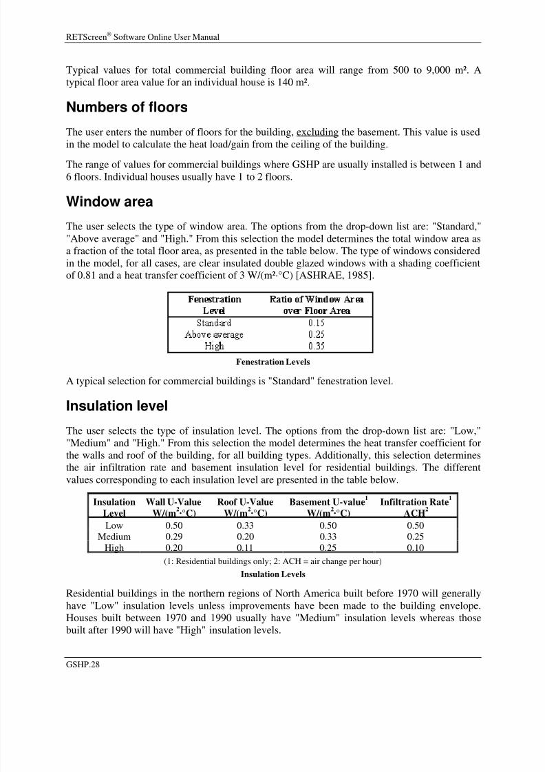
Typical values for total commercial building floor area will range from 500 to 9,000 m². Atypical floor area value for an individual house is 140 m².
Numbers of floors
The user enters the number of floors for the building, excluding the basement. This value is usedin the model to calculate the heat load/gain from the ceiling of the building.
The range of values for commercial buildings where GSHP are usually installed is between 1 and6 floors. Individual houses usually have 1 to 2 floors.
Window area
The user selects the type of window area. The options from the drop-down list are: "Standard,""Above average" and "High." From this selection the model determines the total window area asa fraction of the total floor area, as presented in the table below. The type of windows consideredin the model, for all cases, are clear insulated double glazed windows with a shading coefficientof 0.81 and a heat transfer coefficient of 3 W/(m²·°C) [ASHRAE, 1985].
Fenestration Levels
A typical selection for commercial buildings is "Standard" fenestration level.
Insulation level
The user selects the type of insulation level. The options from the drop-down list are: "Low,""Medium" and "High." From this selection the model determines the heat transfer coefficient forthe walls and roof of the building, for all building types. Additionally, this selection determinesthe air infiltration rate and basement insulation level for residential buildings. The differentvalues corresponding to each insulation level are presented in the table below.
InsulationLevel
Wall U-ValueW/(m
2·°C)
Roof U-ValueW/(m
2·°C)
Basement U-value1
W/(m2·°C)
Infiltration Rate1
ACH2
Low 0.50 0.33 0.50 0.50
Medium 0.29 0.20 0.33 0.25High 0.20 0.11 0.25 0.10
(1: Residential buildings only; 2: ACH = air change per hour)
Insulation Levels
Residential buildings in the northern regions of North America built before 1970 will generallyhave "Low" insulation levels unless improvements have been made to the building envelope.Houses built between 1970 and 1990 usually have "Medium" insulation levels whereas thosebuilt after 1990 will have "High" insulation levels.
GSHP.28

8/3/2019 GSHP3
http://slidepdf.com/reader/full/gshp3 29/104
RETScreen® Ground-Source Heat Pump Project Model
Commercial buildings will tend to have somewhat lower insulation levels than residentialbuildings of the same age. Insulation levels for industrial buildings can vary widely but are oftenlower than either residential or commercial.
Occupancy type
The user selects the occupancy type. The options from the drop-down list are: "Daytime," "Nighttime" and "Continuous." This selection determines the amount of time during which the buildingis occupied. "Daytime" occupancy corresponds to a schedule of 07:00-19:00 while "Nighttime"occupancy is from 19:00-07:00. The model uses these schedules to calculate the sensible andlatent heat gains from occupants in the building as well as fresh air ventilation rates. Eachoccupant is considered as having 75 W of sensible and 75 W of latent heat losses and requires20 L/s of fresh air. For all commercial buildings, the occupant density is 1 person per 10 m²while industrial buildings have a density of 1 person per 50 m².
Typical commercial buildings have "Daytime" occupancy. Industrial occupancy type can varyfrom "Daytime" to "Continuous." "Nighttime" occupancy is less frequent but can sometimes
apply to commercial buildings.
Equipment and lighting usage
The user selects the type of equipment and lighting use. The options from the drop-down list are:"Light," "Moderate" and "Heavy." This selection determines the amount of internal heat gainsfor the building. Commercial and industrial buildings are characterised by much higher internalheat gains than residential ones. The sources of these internal gains can be very numerous butlighting and office equipment, also called plug loads, usually amount for the majority of internalheat gains in commercial buildings. Industrial buildings necessitate a case by case analysis sincetheir sources of internal gains can be quite variable (compressors, motors, process equipment,
etc.). The model uses the selected heat gains in combination with the type of occupancy toevaluate the total daily internal heat gains. The table below presents the heat loads associatedwith each of the three available options.
Equipment &Lighting Usage
Equipment Heat LoadW/m
2Lighting Heat Load
W/m2
Light 5 5Moderate 10 15
Heavy 20 25 Internal Heat Gain Levels
The typical values of equipment and lighting usage will vary depending on the use of thebuilding under consideration. For example, typical office buildings have "Moderate" equipmentand lighting usage, schools will have "Light" usage while hospitals will have "Heavy" usage.Industrial buildings will generally have "Moderate" to "Heavy" equivalent internal gains. Theterm "equivalent" is used in the case of industrial buildings since their actual sources can bedifferent than office equipment or lighting. However, the user should evaluate, wheneverpossible, the internal gains per m² and select the option that best matches these gains.
GSHP.29

8/3/2019 GSHP3
http://slidepdf.com/reader/full/gshp3 30/104
RETScreen® Software Online User Manual
Foundation type
The user selects the foundation type. The two options in the drop-down list are: "Full basement"and "Slab on grade." This selection is used in the model to evaluate the foundation heat losses forresidential buildings. Selecting "Full basement" leads to higher heating loads but has a smaller
impact on cooling loads.
Heat loss through the foundation is the prime heat source for simple slab on grade with groundfrost heat pump (GFHP) chilled in permafrost. Heat gain to the ground from buildingfoundations must be considered when calculating ground collector of chilled foundations forbuildings on permafrost. Heat must be extracted at the same rate as foundation heat loss tomaintain a constant ground temperature and long term balance.
Annual cooling energy demand
If the user selected the "Energy use data" option, then the value for "Annual cooling energydemand" is entered directly by the user.
The annual cooling energy demand is the amount of energy required to cool the building. Thisvalue is used to generate the equations shown in the Heating and Cooling Load Relationshipswhich are then used to recalculate the building's actual cooling energy use. The annual coolingenergy demand is used in combination with the base case air-conditioner seasonal Coefficient Of Performance (COP) to calculate the baseline cost for cooling.
Units switch: The user can choose to express the energy in different units by selecting amongthe proposed set of units: "GWh," "Gcal," "million Btu," "GJ," "therm," "kWh," "hp-h," "MJ."This value is for reference purposes only and is not required to run the model.
Note: At this point, the user should return to the Energy Model worksheet.
Building design heating load
If the user selected the "Descriptive data" option, the model calculates the building's designheating load, based on the "Heating design temperature" (entered in the site conditions section)and the various building parameters selected by the user.
The model uses the design heating load to determine the suggested heat pump capacity, incombination with the design cooling load. The calculated load corresponds to the block heatingload for all types of buildings. The block load refers to the peak load occurring in a building at aspecific time under design temperature conditions. For example, in a building with many zones
(independent thermostats), the summation of each zone's heating load can exceed the block heating load since these loads might not happen concurrently (for occupancy, exposure, solargain or other reasons). For a residential building, block heating load is usually the summation of all room loads under the same design conditions.
Typical values for building heating load range from 20 to 120 W/m².
GSHP.30

8/3/2019 GSHP3
http://slidepdf.com/reader/full/gshp3 31/104
RETScreen® Ground-Source Heat Pump Project Model
Units switch: The user can choose to express the load in different units by selecting among theproposed set of units: "MW," "million Btu/h," "boiler hp," "ton (cooling)," "hp," "W." This valueis for reference purposes only and is not required to run the model.
Building heating energy demand
If the user selected the "Descriptive data" option, the model calculates the building's heatingenergy demand, based on parameters selected by the user.
The building's annual heating energy demand is the amount of energy required to heat thebuilding. This value is used to generate the equations shown in the Heating and Cooling LoadRelationships figure which are then used to recalculate the building's actual heating energy use.
The "Building heating energy demand" is used in combination with the base case heating systemseasonal efficiency to calculate the baseline cost for heating. Typical commercial buildings innorthern regions of North America will use between 50 to 250 kWh/m²/yr. Residential buildingswill use approximately 120 kWh/m²/yr for heating or approximately 60% of their total annual
energy use.
Units switch: The user can choose to express the energy in different units by selecting amongthe proposed set of units: "GWh," "Gcal," "million Btu," "GJ," "therm," "kWh," "hp-h," "MJ."This value is for reference purposes only and is not required to run the model.
Building design cooling load
If the user selected the "Descriptive data" option the model calculates the building's designcooling load, based on the "Cooling design temperature" (entered in the site conditions section)and the various building parameters selected by the user.
The model uses the design cooling load to determine the suggested heat pump capacity, incombination with the design heating load. The calculated load corresponds to the block coolingload for each type of building selected. The block load refers to the peak load occurring in abuilding at a specific time under design temperature conditions. For example, in a building withmany zones (independent thermostats), the summation of each zone's cooling load can exceedthe block cooling load since these loads might not happen concurrently (for occupancy,exposure, solar gain or other reasons). For a residential building, block cooling load is usuallythe summation of all room loads under the same design conditions.
Cooling loads are project specific and depend on all building parameters selected in addition tothe site conditions and the building's use. The values will generally vary from 50 W/m² for
residential buildings in cool climates to 200 W/m² or more for commercial buildings in hotclimate with high internal gains.
Units switch: The user can choose to express the load in different units by selecting among theproposed set of units: "MW," "million Btu/h," "boiler hp," "ton (cooling)," "hp," "W." This valueis for reference purposes only and is not required to run the model.
GSHP.31

8/3/2019 GSHP3
http://slidepdf.com/reader/full/gshp3 32/104
RETScreen® Software Online User Manual
Building cooling energy demand
If the user selected the "Descriptive data" option, the model calculates the building's coolingenergy demand, based on parameters selected by the user.
The building's annual cooling energy demand is the amount of energy required to cool thebuilding. This value is used to generate the equations shown in the Heating and Cooling LoadRelationships figure which are then used to recalculate the building's actual cooling energy use.The "Building cooling energy demand" value is used in combination with the base case air-conditioner seasonal Coefficient Of Performance (COP) to calculate the baseline cost forcooling.
Units switch: The user can choose to express the energy in different units by selecting amongthe proposed set of units: "GWh," "Gcal," "million Btu," "GJ," "therm," "kWh," "hp-h," "MJ."This value is for reference purposes only and is not required to run the model.
Note: At this point, the user should return to the Energy Model worksheet.
Design heating load
If the user selected the "Energy use data" option, then the value for "Design heating load" isentered directly by the user. This value will depend on the design temperature for the specificlocation and on the building insulation efficiency.
The model uses the design heating load to determine the suggested heat pump capacity, incombination with the design cooling load. The entered load corresponds to the block heatingload for all types of buildings. The block load refers to the peak load occurring in a building at aspecific time under design temperature conditions. For example, in a building with many zones(independent thermostats), the summation of each zone's heating load can exceed the block heating load since these loads might not happen concurrently (for occupancy, exposure, solargain or other reasons). For a residential building, block heating load is usually the summation of all room loads under the same design conditions.
Typical values for building heating load range from 20 to 120 W/m².
Units switch: The user can choose to express the load in different units by selecting among theproposed set of units: "MW," "million Btu/h," "boiler hp," "ton (cooling)," "hp," "W." This valueis for reference purposes only and is not required to run the model.
Annual heating energy demand
If the user selected the "Energy use data" option, then the value for "Annual heating energydemand" is entered directly by the user.
The annual heating energy demand is the amount of energy required to heat the building. Thisvalue is used to generate the equations shown in the Heating and Cooling Load Relationshipsfigure which are then used to recalculate the building's actual heating energy use.
GSHP.32

8/3/2019 GSHP3
http://slidepdf.com/reader/full/gshp3 33/104
RETScreen® Ground-Source Heat Pump Project Model
The annual heating energy demand is used in combination with the base case heating systemseasonal efficiency to calculate the baseline cost for heating. Typical commercial buildings innorthern regions of North America will use between 50 to 250 kWh/m²/yr. Residential buildingswill use approximately 120 kWh/m²/yr for heating or approximately 60% of their total annualenergy use.
Units switch: The user can choose to express the energy in different units by selecting amongthe proposed set of units: "GWh," "Gcal," "million Btu," "GJ," "therm," "kWh," "hp-h," "MJ."This value is for reference purposes only and is not required to run the model.
Design cooling load
If the user selected the "Energy use data" option, then the value for "Design cooling load" isentered directly by the user. This value will depend on the design temperature for the specificlocation and on building insulation efficiency.
The model uses the design cooling load to determine the suggested heat pump capacity, in
combination with the design heating load. The entered load corresponds to the block coolingload for each type of building selected. The block load refers to the peak load occurring in abuilding at a specific time under design temperature conditions. For example, in a building withmany zones (independent thermostats), the summation of each zone's cooling load can exceedthe block cooling load since these loads might not happen concurrently (for occupancy,exposure, solar gain or other reasons). For a residential building, block cooling load is usuallythe summation of all room loads under the same design conditions.
Cooling loads are project specific and depend on all building parameters selected in addition tothe site conditions and the building's use. The values will generally vary from 50 W/m² forresidential buildings in cool climates to 200 W/m² or more for commercial buildings in hot
climate with high internal gains.Units switch: The user can choose to express the load in different units by selecting among theproposed set of units: "MW," "million Btu/h," "boiler hp," "ton (cooling)," "hp," "W." This valueis for reference purposes only and is not required to run the model.
GSHP.33

8/3/2019 GSHP3
http://slidepdf.com/reader/full/gshp3 34/104
RETScreen® Software Online User Manual
Cost Analysis1
As part of the RETScreen Clean Energy Project Analysis Software, the Cost Analysis worksheetis used to help the user estimate costs associated with a ground-source heat pump project. Thesecosts are addressed from the initial, or invesment, cost standpoint and from the annual, or
recurring, cost standpoint. The user may refer to the RETScreen Online Product Database forsupplier contact information in order to obtain prices or other information required.
The selection of a cost-effective GSHP system will depend of many factors, although someguidelines can be used to orient this selection process.
• GWHPS: When groundwater is available in sufficient quantities with adequate quality,and environmental regulations permit this type of installation, such a system should beconsidered. GWHP systems will generally be more financially attractive for largerbuildings since the cost of the groundwater wells (supply and injection) does not riselinearly with capacity.
• Vertical GCHPs: Vertical Ground-coupled heat pump systems are usually limited tobuildings with six stories or less due to the static pressure limitations for the GHX pipes[ASHRAE, 1995]. It is possible to use stronger GHX pipes but they are more expensiveand difficult to work with. Generally, when a system's cooling capacity exceeds 350 to700 kW, the surface of a typical parking lot will not be sufficient to accommodate theGHX without supplemental heat rejection. Vertical GCHPs are common in residentialapplications, particularly where drilling costs are low.
• Horizontal GCHPs: Horizontal Ground-coupled heat pump systems do not have theheight limitations and pipe requirements imposed on vertical systems. However, theyrequire larger land area and, generally, when the system's cooling capacity exceeds 35 to
70 kW, the surface of a typical parking lot will not be sufficient to accommodate theGHX without supplemental heat rejection. Horizontal systems can usually offer thelowest initial costs but will also have lower seasonal efficiencies because of lower groundtemperature. These characteristics are often well suited for residential applications.
The most cost-effective installations of ground-source heat pump systems normally occur in newconstruction, where the building's design can be planned to maximise GSHP system benefits, asmentioned in the background section of this manual. Retrofit installations should also beconsidered but may have longer payback periods. In case of retrofit situations where the buildingheating/cooling system is to be upgraded/replaced, the financial benefits of GSHP projects willimprove due to the "credits" described below.
For all ground-source heat pump projects, "credits" for material and labour costs that would havebeen spent on a "conventional" heating and cooling system have to be accounted for. The user
1 A reminder to the user that the range of values for cost items mentioned in the manual are for a 2000 baselineyear in Canadian dollars. Some of this data may be time sensitive so the user should verify current values whereappropriate. (The approximate exchange rate from Canadian dollars to United States dollars and to the Euro was0.68 as of January 1, 2000).
GSHP.34

8/3/2019 GSHP3
http://slidepdf.com/reader/full/gshp3 35/104
RETScreen® Ground-Source Heat Pump Project Model
will have to determine these initial costs in order to obtain a plausible financial evaluation of theGSHP project. These credits will also apply to engineering and design, some development costsand some annual costs. Grey input cells are provided to allow project decision-makers to keeptrack of credit items when preparing the project cost analysis.
Type of analysisThe user selects the type of analysis from the drop-down list. For a "Pre-feasibility analysis," lessdetailed and lower accuracy information is typically required while for a "Feasibility analysis,"more detailed and higher accuracy information is usually required.
To put this in context, when funding and financing organisations are presented with a request tofund an energy project, some of the first questions they will likely ask are "how accurate is theestimate, what are the possibilities for cost over-runs and how does it compare financially withother options?" These are very difficult to answer with any degree of confidence, since whoeverprepared the estimate would have been faced with two conflicting requirements:
• Keep the project development costs low in case funding cannot be secured, or in case theproject proves to be uneconomic when compared with other energy options.
• Spend additional money and time on engineering to more clearly delineate potentialproject costs and to more precisely estimate the amount of energy produced or energysaved.
To overcome, to some extent, such conflicts, the usual procedure is to advance the projectthrough the following four stages:
• Pre-feasibility analysis
• Feasibility analysis
• Development (including financing) and engineering
• Construction and commissioning
Each stage could represent an increase of a magnitude or so in expenditure and a halving of theuncertainty in the project cost-estimate. This process is illustrated, for hydro projects, in theAccuracy of Project Cost Estimates figure [Gordon, 1989].
At the completion of each step, a "go or no go" decision is usually made by the project proponentas to whether to proceed to the next step of the development process. High quality, but low-cost,pre-feasibility and feasibility studies are critical to helping the project proponent "screen out"
projects that do not make financial sense, as well as to help focus development and engineeringefforts prior to construction. The RETScreen Clean Energy Project Analysis Software can beused to prepare both the initial pre-feasibility analysis and the more detailed feasibility analysis.
GSHP.35

8/3/2019 GSHP3
http://slidepdf.com/reader/full/gshp3 36/104
RETScreen® Software Online User Manual
Accuracy of Project Cost Estimates [Gordon, 1989]
Currency
To perform a RETScreen project analysis, the user may select a currency of their choice from the"Currency" cell in the Cost Analysis worksheet.
The user selects the currency in which the monetary data of the project will be reported. Forexample, if the user selects "$," all monetary related items are expressed in $.
Selecting "User-defined" allows the user to specify the currency manually by entering a name orsymbol in the additional input cell that appears adjacent to the currency switch cell. The currencymay be expressed using a maximum of three characters ($US, £, ¥, etc.). To facilitate thepresentation of monetary data, this selection may also be used to reduce the monetary data by afactor (e.g. $ reduced by a factor of a thousand, hence k$ 1,000 instead of $ 1,000,000).
If "None" is selected, all monetary data are expressed without units. Hence, where monetary datais used together with other units (e.g. $/kWh) the currency code is replaced with a hyphen(-/kWh).
The user may also select a country to obtain the International Standard Organisation (ISO) three-letter country currency code. For example, if Afghanistan is selected from the currency switchdrop-down list, all project monetary data are expressed in AFA. The first two letters of the
GSHP.36

8/3/2019 GSHP3
http://slidepdf.com/reader/full/gshp3 37/104
RETScreen® Ground-Source Heat Pump Project Model
country currency code refer to the name of the country (AF for Afghanistan), and the third letterto the name of the currency (A for Afghani).
For information purposes, the user may want to assign a portion of a project cost item in asecond currency, to account for those costs that must be paid for in a currency other than thecurrency in which the project costs are reported. To assign a cost item in a second currency, the
user must select the option "Second currency" from the "Cost references" drop-down list cell.
Some currency symbols may be unclear on the screen (e.g. €); this is caused by the zoom settingsof the sheet. The user can then increase the zoom to see those symbols correctly. Usually,symbols will be fully visible on printing even if not fully appearing on the screen display.
Cost references
The user selects the reference (from the Cost Analysis worksheet) that will be used as a guidelinefor the estimation of costs associated with the implementation of the project. This feature allowsthe user to change the "Quantity Range" and the "Unit Cost Range" columns. The options from
the drop-down list are: "Canada - 2000," "None," "Second currency" and a selection of 8 user-defined options ("Enter new 1," "Enter new 2," etc.).
If the user selects "Canada - 2000" the range of values reported in the "Quantity Range" and"Unit Cost Range" columns are for a 2000 baseline year, for projects in Canada and in Canadiandollars. This is the default selection used in the built-in example in the original RETScreen file.
Selecting "None" hides the information presented in the "Quantity Range" and "Unit CostRange" columns. The user may choose this option, for example, to minimise the amount of information printed in the final report.
If the user selects "Second currency" two additional input cells appear in the next row: "Second
currency" and "Rate: 1st currency/2nd currency." In addition, the "Quantity Range" and "UnitCost Range" columns change to "% Foreign" and "Foreign Amount," respectively. This optionallows the user to assign a portion of a project cost item in a second currency, to account forthose costs that must be paid for in a currency other than the currency in which the project costsare reported. Note that this selection is for reference purposes only, and does not affect thecalculations made in other worksheets.
If "Enter new 1" (or any of the other 8 selections) is selected, the user may manually enterquantity and cost information that is specific to the region in which the project is located and/orfor a different cost base year. This selection thus allows the user to customise the information inthe "Quantity Range" and "Unit Cost Range" columns. The user can also overwrite "Enter new1" to enter a specific name (e.g. Japan - 2001) for a new set of unit cost and quantity ranges. Theuser may also evaluate a single project using different quantity and cost ranges; selecting a newrange reference ("Enter new 1" to "Enter new 8") enables the user to keep track of different costscenarios. Hence the user may retain a record of up to 8 different quantity and cost ranges thatcan be used in future RETScreen analyses and thus create a localised cost database.
GSHP.37

8/3/2019 GSHP3
http://slidepdf.com/reader/full/gshp3 38/104
RETScreen® Software Online User Manual
Second currency
The user selects the second currency; this is the currency in which a portion of a project cost itemwill be paid for in the second currency specified by the user. The second currency option isactivated by selecting "Second currency" in the "Cost references" drop-down list cell. This
second unit of currency is displayed in the "Foreign Amount" column.
If the user selects "$," the unit of currency shown in the "Foreign Amount" column is "$."
Selecting "User-defined" allows the user to specify the currency manually by entering a name orsymbol in the additional input cell that appears adjacent to the currency switch cell. The currencymay be expressed using a maximum of three characters ($US, £, ¥, etc.). To facilitate thepresentation of monetary data, this selection may also be used to reduce the monetary data by afactor (e.g. $ reduced by a factor of a thousand, hence k$ 1,000 instead of $ 1,000,000).
If "None" is selected, no unit of currency is shown in the "Foreign Amount" column.
The user may also select a country to obtain the International Standard Organisation (ISO) three-letter country currency code. For example, if Afghanistan is selected from the currency switchdrop-down list, the unit of currency shown in the "Foreign Amount" column is "AFA." The firsttwo letters of the country currency code refer to the name of the country (AF for Afghanistan),and the third letter to the name of the currency (A for Afghani).
Some currency symbols may be unclear on the screen (e.g. €); this is caused by the zoom settingsof the sheet. The user can then increase the zoom to see those symbols correctly. Usually,symbols will be fully visible on printing even if not fully appearing on the screen display.
Rate: 1st currency/2nd currency
The user enters the exchange rate between the currency selected in "Currency" and the currencyselected in "Second currency." The exchange rate is used to calculate the values in the "ForeignAmount" column. Note that this selection is for reference purposes only, and does not affect thecalculations made in other worksheets.
For example, the user selects the Afghanistan currency (AFA) as the currency in which themonetary data of the project is reported (i.e. selection made in "Currency" input cell) - this is the1st currency. The user then selects United States currency (USD) from the "Second currency"input cell - this is the 2nd currency. The user then enters the exchange rate in the "Rate:AFA/USD" input cell i.e. the amount of AFA needed to purchase 1 USD. Using this feature theuser can then specify what portion (in the "% Foreign" column) of a project cost item's costs will
be paid for in USD.
% Foreign
The user enters the percentage of an item's costs that will be paid for in the second currency. Thesecond currency is selected by the user in the "Second currency" cell.
GSHP.38

8/3/2019 GSHP3
http://slidepdf.com/reader/full/gshp3 39/104
RETScreen® Ground-Source Heat Pump Project Model
Foreign Amount
The model calculates the amount of an item's costs that will be paid for in the second currency.This value is based on the exchange rate and the percentage of an items costs that will be paid forin the second currency, as specified by the user.
Initial Costs
The initial costs associated with the implementation of a ground-source heat pump project aredetailed below. The major categories include costs for preparing a feasibility study, performingthe project development functions, completing the necessary engineering, purchasing andinstalling the energy equipment, construction of the balance of system and costs for any othermiscellaneous items.
Feasibility Study
Once a potentially cost-effective ground-source heat pump project has been identified throughthe RETScreen pre-feasibility analysis process, a more detailed feasibility analysis study may berequired. This is particularly the case for larger projects, typically larger than 100 kW. Feasibilitystudies typically include such items as a site investigation, a soil/hydrology assessment, anenvironmental assessment, a preliminary project design, including loop sizing and layout, adetailed cost estimate, and a final report. Feasibility study project management and travel costsare also normally incurred. These costs are detailed in the section below.
For small projects, such as small commercial systems, the cost of the feasibility study, relative tothe cost of the ground-source heat pump system, may not be justified. In this case the projectproponent may choose to go directly to the engineering stage (combining some steps from thefeasibility and development stages).
Note: The RETScreen Clean Energy Project Analysis Software can also be used to prepare theFeasibility Study.
Site investigation
When a GSHP system is being considered for an existing building, a site visit may be required toevaluate the site and building conditions and their suitability for installing the proposed GSHPsystem. For new construction, this visit may also be required to evaluate the potential of theterrain to receive the earth connection (GHX or water wells).
The visits should be conducted with a GSHP project expert and should allow for the refinementof assumptions made during the pre-feasibility study. During the visits elements such as buildingphysical characteristics (areas, insulation levels, etc.), documentation of the existing buildingheating and cooling systems (for retrofit applications), location of the potential earth loop and theowner's right of access to the proposed GHX location or to the groundwater resources should bedocumented. Site visit time includes the time required to arrange meetings, survey the site,obtain the necessary information and any travel time (but not travel expenses - see "Travel andaccommodation" below).
GSHP.39

8/3/2019 GSHP3
http://slidepdf.com/reader/full/gshp3 40/104
RETScreen® Software Online User Manual
For a retrofit project, the time required for a site survey, detailed building and site analysis variesaccording to the size of the building involved and the complexity of the existing heating andcooling system. Obtaining energy consumption data can sometimes add to the time required. Thetime required to collect the data prior to and during the site visit typically falls between 14 to21 hours (travel time extra) at a rate of approximately $40/h to $100/h. For new construction,
where building data can be extracted from architectural or engineering drawings, the timerequired typically falls between 7 to 14 hours (travel time extra) at the same rate.
Site investigations involving GSHPs in permafrost-related applications are usually limited toparticular applications including building foundation chilling or specialised energy transferprojects. Such projects are normally incorporated in new construction feasibility studies andrequire case to case cost evaluation.
Soil/hydrology assessment
While most sites are suitable for GSHP system installations, in some cases specific land orsubsurface features may result in increased equipment and/or installation costs. Furthermore, in
some cases a site may be judged inappropriate for any type of GSHP system. For these reasons, asoil or hydrologic assessment, depending on the proposed GSHP system type, is needed. Theinformation collected during the assessment, and its cost, will depend on the GSHP system type.
GWHP systems will usually require the most extensive evaluation. In this case, ahydrogeological assessment has to be conducted. A typical study should be conducted by aqualified hydrogeologist and should include:
• Establishing all regulations pertinent to the installation of a groundwater system at theproposed site;
• Reviewing existing geological/hydrogeological information for the site location; and
• Subsurface investigation through test wells.
The number of test wells required is linked to the size of the proposed GWHP system. Forbuildings less than 3,000 m², one test well is sufficient. For larger buildings, at least two testwells should be drilled.
For GCHP systems, a geotechnical investigation can be sufficient to determine the site'ssuitability. However, for vertical GCHP systems, it is often valuable to have a hydrogeologicalinvestigation done. The information from the latter survey will also insure that the groundwaterquality is documented prior to the installation of the vertical GCHP. This should help prevent thesystem's owner from being held responsible for any groundwater contamination that predated the
vertical GCHP installation. A geotechnical survey for vertical GCHPs consists of test holesdrilled at least 15 m below the deepest planned GHX hole. For buildings of less than 3,000 m²,one test hole is sufficient. For larger buildings, two test holes should be drilled. Horizontalsystem geotechnical investigations consist of test pits to provide knowledge of the subsurfaceconditions. For GHX of less than one hectare in area, a minimum of four test pits isrecommended. For GHX larger than two hectares, two test pits per hectare is recommended[ASHRAE, 1995].
GSHP.40

8/3/2019 GSHP3
http://slidepdf.com/reader/full/gshp3 41/104
RETScreen® Ground-Source Heat Pump Project Model
The time required to carry out a soil/hydrology assessment is typically 60 to 120 hours forGWHP systems, 35 to 80 hours for vertical GCHP systems and 20 to 50 hours for horizontalGCHP systems. Typical rates for hydrogeologists or geological technicians range from $40/h to$100/h. In addition to these costs, the user should add the cost of drilling wells or boreholes ortrenching of test pits.
Should soil/hydrologic assessments for isolated areas and permafrost zones be required, thetypical assessment rate equals 1 to 1.5 times the conventional rate. Refer to the travel andaccommodation section for additional costs. As is the case for site investigation, hydrogeologicalassessment may only be carried out when climatic conditions permit it.
Preliminary design
A preliminary design that combines the above information is required. In order to reduce costs,the preliminary design should be done using standard methods and existing computer designtools. The preliminary design should allow for more precise estimates of the building's loads, azone by zone selection for the heat pumps and a more precise determination of the GHX size or
groundwater flow requirement.
The cost for preparing a preliminary design will be strongly dependent on a building's size andheating and cooling system's complexity. The time required to complete the design can rangefrom 5 to 40 hours at a rate of approximately $60/h to $100/h.
Preliminary design using GSHP in permafrost-related applications usually is limited to specificapplications. Such design requires case to case evaluation. Required time will vary while theapproximate rate should remain the same.
Detailed cost estimate
The detailed cost estimate for the proposed GSHP project is based on the results of thepreliminary design and other investigations carried out during the feasibility study. The cost of preparing the detailed cost estimate is calculated based on an estimate of the time required byexperts to complete the necessary work.
Engineering services for completing a detailed GSHP project cost estimate will range from $60/hto $100/h. The number of hours required to complete the cost estimate will range between 7 to35 hours depending on the size of the project and the acceptable level of risk.
Report preparation
A summary report should be prepared which describes the feasibility study, its findings andrecommendations. The written report will contain data summaries, charts, tables and illustrationsthat clearly describe the proposed project. This report should be in sufficient detail regardingcosts, performance and risks to enable project lenders and other decision-makers to evaluate themerits of the project.
The cost of the report preparation is calculated based on an estimate of the time required by aprofessional to complete the necessary work, and should also include the time required to
GSHP.41

8/3/2019 GSHP3
http://slidepdf.com/reader/full/gshp3 42/104
RETScreen® Software Online User Manual
manage the overall feasibility study preparation. Typically, 16 to 32 hours are required at a rateof between $60/h to $100/h.
Travel and accommodation
This cost item includes all travel related costs (excluding time) required to prepare all sections of the feasibility study by the various members of the feasibility study team. These expensesinclude such items as airfare, car rental, lodging and per diem rates for each trip required. Forlocal travel, a supplier may not charge for time and expenses. For isolated areas, where air travelis time consuming and expensive, it may be better to include more than one potential project inthe feasibility study to spread the site visit costs over a number of projects and not just onebuilding.
In case of isolated areas, particularly permafrost zones, rates for air travel will vary considerably.Airfares are typically twice (up to ten times in isolated permafrost areas) those for similardistances in populated areas. Since travel is a large component of the cost of doing work inisolated areas and the range of cost so variable, it is advisable to contact a travel agent with
experience in arranging such travel. Accommodation rates are typically twice the going rate formodest accommodation in populated areas. Typical rates for modest hotel rooms can range from$180 to $250 per day in the more isolated areas (per diem can vary between $35 to $70).
Other
These input cells are provided to allow the user to enter cost or credit items that are not includedin the information provided in the above cost category. The user must enter a positive numericalvalue in the "Unit Cost" column.
A cost item may be entered in the grey input cell as "Other." The user then selects "Cost" from
the drop-down list in the unit column. The user can input both a quantity amount and unit cost.This item is provided to allow for project, technology and/or regional differences not specificallycovered in the generic information provided.
A credit item may be entered in the grey input cell as "Credit." The user then selects "Credit"from the drop-down list in the unit column. The project may be credited for material and/orlabour costs that would have been spent on the base case, or conventional, energy system. Theuser can input both a quantity amount and unit cost. Note that the credit item is expressed as anegative value in the "Amount" column.
Development
Once a potential ground-source heat pump project has been identified through the feasibilitystudy to be desirable to implement, project development activities may follow. For someprojects, the feasibility study, development and engineering activities may proceed in parallel,depending on the risk and return acceptable to the project proponent.
For GSHP projects, there are a number of possible project developers. Currently, a commonapproach is for the client to be the building owner with the developer being a local GSHPsupplier who provides complete design/build services. The general contractor may also be the
GSHP.42

8/3/2019 GSHP3
http://slidepdf.com/reader/full/gshp3 43/104
RETScreen® Ground-Source Heat Pump Project Model
developer, purchasing the GSHP system on behalf of the building owner. It is also possible thatan Energy Services Company (ESCO) could be the project developer, and take charge of financing and installing the GSHP system and in return receive a portion of the annual energysavings. Estimating the costs of the development phase will depend on the particulardevelopment arrangement established. Items here include costs for permits and approvals, land
survey, project financing, development phase project management and any development relatedtravel costs. These costs are detailed in the section below.
Permits and approvals
A number of permits and approvals may be required from local authorities for the construction of the project. The cost of acquiring the necessary permits and approvals is calculated based on anestimate of the time required to complete the necessary work. These agencies may include localbuilding and electrical inspectors, fire safety inspectors, and an environmental regulatingauthority.
In certain isolated areas, local native band council approval may also be required. Added relative
costs are minor, however time needed to obtain such approvals has to be accounted for.
The time required depends on the number of agencies involved and what is specifically requiredto meet their rules and regulations. The time requirement is typically 4 to 12 hours at ratesranging from $40/h to $100/h for project development staff. The user can also add to the numberof hours, or unit costs, an amount to cover the actual cost of the permit. Permit costs are usuallyminor relative to the total project cost.
Land survey
Given the potentially large terrain occupied by the GHX in some GSHP systems, a land survey
may be required to insure that the GHX is located on premises belonging to the building's owner.
Typically, the costs to survey one simple lot of 1 to 10 hectares are of the order of $750. The costmay vary if travel and accommodation costs are billed by the surveyor. Typically, a land surveywill take between 0 to 30 hours at a rate of $50/h to $80/h.
Land surveying in isolated/permafrost areas may typically take the same amount of time,however travel costs, travel time and accommodation expenses have to be considered. Rates of $80 to $120 may apply.
Project financing
The time and effort required to arrange project financing will vary depending upon the projectdeveloper and client relationship. In most cases, where the client is the building owner and thedeveloper is the product supplier, the project financing costs attributable to the project areminimal. The building owner will usually finance the project out of capital or O&M budgets andthe product supplier will provide in-kind support as required to help arrange the client projectfinancing. In the case of an ESCO developed project much more effort will likely be required toarrange financing, negotiate an energy services contract with the building owner and preparelegal documents.
GSHP.43

8/3/2019 GSHP3
http://slidepdf.com/reader/full/gshp3 44/104
RETScreen® Software Online User Manual
The cost to obtain project financing will range from 8 to 24 hours at a rate of between $60/h to$180/h. The lower end of the range is for building owner/product supplier developed projects.The higher end of the range applies to ESCO type projects.
Project management
The project management cost item should cover the estimated expenses of managing all phasesof the development of the project (excluding construction supervision).
The elapsed time for the development of a ground-source heat pump project is relatively short.Depending on the project scale, an entire project can be easily developed within a year withactual construction time only taking a few weeks. The project development management timewill usually take between 20 to 40 hours at rates of between $50/h to $100/h.
Travel and accommodation
This cost item includes all travel related costs (excluding time) required to develop the project.
Other
These input cells are provided to allow the user to enter cost or credit items that are not includedin the information provided in the above cost category. The user must enter a positive numericalvalue in the "Unit Cost" column.
A cost item may be entered in the grey input cell as "Other." The user then selects "Cost" fromthe drop-down list in the unit column. The user can input both a quantity amount and unit cost.This item is provided to allow for project, technology and/or regional differences not specificallycovered in the generic information provided.
A credit item may be entered in the grey input cell as "Credit." The user then selects "Credit"from the drop-down list in the unit column. The project may be credited for material and/orlabour costs that would have been spent on the base case, or conventional, energy system. Theuser can input both a quantity amount and unit cost. Note that the credit item is expressed as anegative value in the "Amount" column.
Engineering
The engineering phase includes costs for the GSHP system design, tenders and contracting, andconstruction supervision. If the project is awarded on a design/build basis, then all of these costs
would be included in prices provided by the equipment supplier or contractor responsible for theproject. If the project is awarded by tender based on specifications prepared by a consultant, thenthere will be engineering charges from the consultant overseeing the project and perhaps theequipment supplier.
GSHP.44

8/3/2019 GSHP3
http://slidepdf.com/reader/full/gshp3 45/104
RETScreen® Ground-Source Heat Pump Project Model
GSHP system design
The GSHP system design includes the time required to design the GHX, or water wells, detailedlayout, piping, pumping and electrical arrangement as well as the detailed design of the heatpump system and any modifications to an existing building's systems. This step includes
preparing design drawings and specifications. For small GSHP systems with standardconfigurations, generic installation drawings can sometimes be used to minimise this cost.
The time required to prepare the system's design and detailed drawings falls between 5 to80 hours. The lower end of the range corresponds to small commercial systems, barely largerthan residential installations while the upper end of the scale corresponds to larger commercialsystems. GSHP design fees usually range from $40/h to $100/h.
GSHP design used in permafrost-related applications usually is limited to specialisedapplications. Such design requires case to case evaluation. Required time will vary whileapproximate rates should remain the same.
Tenders and contracting
Upon completion of the various engineering tasks, tender documents may be required by theproject developer. They are prepared for the purpose of selecting contractors to undertake thework. Once tenders are released, the contracting process is required to both negotiate andestablish contracts for the completion of the project.
The time required to produce a set of bid documents will vary depending upon the complexityand the size of the project. If bid documents are required 20 to 40 hours at rates of $40/h to$100/h are possible.
Construction supervision
The construction supervision cost item summarises the estimated costs associated with ensuringthat the project is constructed as designed. Construction supervision is provided either by theconsultant overseeing the project or by the equipment supplier, or by the project manager.Construction supervision involves regular visits to the job site to inspect the installation.
Depending of the project size, this task can take between 15 to 40 hours at rates of $40/h to$100/h. Travel time to the site for construction supervision is in addition to the indicated range.Travel costs should be included in the "Development" section above.
Due to unusually above average travel fees and travel time, construction supervision in
isolated/permafrost areas requires less frequent regular visits, but lengthier stays. Overseeingconstruction from start to finish should also be considered.
Other
These input cells are provided to allow the user to enter cost or credit items that are not includedin the information provided in the above cost category. The user must enter a positive numericalvalue in the "Unit Cost" column.
GSHP.45

8/3/2019 GSHP3
http://slidepdf.com/reader/full/gshp3 46/104
RETScreen® Software Online User Manual
A cost item may be entered in the grey input cell as "Other." The user then selects "Cost" fromthe drop-down list in the unit column. The user can input both a quantity amount and unit cost.This item is provided to allow for project, technology and/or regional differences not specificallycovered in the generic information provided.
A credit item may be entered in the grey input cell as "Credit." The user then selects "Credit"
from the drop-down list in the unit column. The project may be credited for material and/orlabour costs that would have been spent on the base case, or conventional, energy system. Theuser can input both a quantity amount and unit cost. Note that the credit item is expressed as anegative value in the "Amount" column.
Energy Equipment
The energy equipment, as defined here, includes, when applicable, the system's heat pumps,water well pumps, circulating pumps, heat exchanger, anti-freeze solution, drilling, trenching,GHX pipes, valves and fittings and transportation costs. All cost figures are installed costs andinclude overhead and profit. The user may refer to the RETScreen Online Product Database for
supplier contact information in order to obtain prices or other information required.
Some specific cost items such as those for electrical equipment and controls and transportationcosts are not listed in this section. It is assumed that these costs are equivalent to those of aconventional heating and cooling system and have negligible impact on the incremental cost of aGSHP system.
In cases where heavy or specialised construction machinery may be required specifically for theGSHP system, and not locally available such as in certain isolated areas, transportation costsshould be accounted for in the "Other" cost item.
Heat pumps
The baseline unitary cost of a GSHP is approximately $235 per kW of cooling capacity.However, the cost depends on the selected efficiency, as shown in the table below. The user mayrefer to the RETScreen Online Product Database for supplier contact information in order toobtain prices or other information required.
Heat PumpEfficiency Level
Typical Cost$/kW
Standard $235Medium $270
High $330 Cost of Ground-Source Heat Pumps
The total cooling capacity, based on the building's block load, is automatically copied from the Energy Model worksheet. The unit cost may be lower if large heat pumps are used while it maybe higher for smaller ones. A typical standard efficiency heat pump of only 3.5 kW of coolingcapacity can cost over $570 per kW while a 25 kW unit will be about $200 per kW. The usershould keep in mind that commercial systems may require a total installed capacity higher thanthe evaluated block load capacity.
GSHP.46

8/3/2019 GSHP3
http://slidepdf.com/reader/full/gshp3 47/104
RETScreen® Ground-Source Heat Pump Project Model
Well pumps
The cost of well pumps is estimated based on the pump power requirement (in kW). The powerrequirement is calculated in the model and automatically transferred to the Cost Analysis worksheet. The main types of pumps used in GWHPs are submersible pumps and lineshaft
pumps. For smaller systems (15 L/s or less), submersible pumps will usually be the lowest initialcost option. For larger systems, lineshaft pumps usually become more advantageous.
Unit costs of both types of pumps will primarily be sensitive to the pump design flow rate.Typical costs for both types of pumps are presented in the table below.
Flow RateL/s
Submersible$/kW
Lineshaft$/kW
3 $ 1,700 $ 3,40015 $ 750 $ 85030 $ 450 $ 425
Cost of Well Pumps
Circulating pumps
The cost of circulating pumps is estimated based on the pump power requirement (in kW). Thepower requirement is calculated in the model and automatically transferred to the Cost Analysis worksheet. Circulating pumps are required for both GCHP and GWHP systems.
Unit costs of circulating pumps will vary depending on the pump design power demand. Typicalcosts for circulating pumps are presented in the table below.
CapacitykW
Typical Cost$/kW
0.2 $ 1,9001 $ 1,1004 $ 500
10 $ 35020 $ 250 Cost of Circulating Pumps
Circulating fluid
The cost of circulating fluid is estimated based on the volume of antifreeze solution required (incubic meters). The volume is calculated in the model and automatically transferred to the Cost
Analysis worksheet. Any antifreeze solution used in the building loop, either for GCHPs orGWHPs is not considered in the volume calculation done by the model. Only the GHX loopvolume is considered.
It is quite common for GCHPs to reach below freezing temperature conditions during winteroperations. When such cases are likely, an antifreeze solution must be used in the GHX loop.Common antifreeze solutions used are: calcium chloride, ethanol, ethylene glycol, methanol,propylene glycol, potassium acetate, potassium carbonate and sodium chloride.
GSHP.47

8/3/2019 GSHP3
http://slidepdf.com/reader/full/gshp3 48/104
RETScreen® Software Online User Manual
Each type of fluid has its advantages and disadvantages which are well documented [ASHRAE,1995]. The use of antifreeze in GCHPs is regulated by different government agencies in manycountries and proper verification is required before considering any such fluids. The typical cost($/m³) for propylene glycol ranges from $2,400 to $3,000.
It is important to note, that in some areas the use of particular types of antifreeze solutions is not
permitted by local authorities, therefore it is well advised to be well informed about theregulations prior to deciding which fluid to use.
Plate heat exchangers
The plate heat exchanger cost is estimated based on the heat pump system cooling capacity (inkW). The capacity is calculated by the model and automatically transferred to the Cost Analysis worksheet. The most widely used type of heat exchangers in GWHP system is plate type. Theseheat exchangers are efficient, compact, easy to maintain and affordable. The typical costs rangebetween $7/kW to $20/kW of installed cooling capacity depending on heat exchanger size.
Trenching and backfilling
Trenching for a horizontal GHX can be done with a backhoe, a chained excavator, a vibratoryplough or even a bulldozer for large fields. The unit cost of trenching and backfilling can beinfluenced by factors such as trench depth, soil type, presence of obstacles (e.g. boulders) and thenumber of turnarounds. The backfilling process is critical for good GHX performances andintegrity. Backfill material should not contain any large rocks and sand should be used where thepipes are located.
The typical costs for trenching and backfilling, for a 1.8 m deep trench, are presented in the tablebelow. The length of trench is calculated in the model and copied automatically from the Energy
Model worksheet. Permafrost conditions can make trenching costs in isolated areas significantlyhigher. In isolated areas, construction machinery can sometimes be rented locally but rental costsmay be up to 1.5 times standard costs.
Trench Widthm
Typical Cost Range$/m
0.15 $4.00 to $6.000.61 $4.00 to $6.000.91 $5.00 to $9.00
Cost of Trenching and Backfilling (excluding turnarounds)
Typical costs for a turnaround will vary from $40 to $70 per turnaround.
Drilling and grouting
Drilling for vertical GHX or GWHP systems can be done with conventional drilling equipmentsuch as rotary drills, cable tool drills and air drills. The unit cost of drilling is closely linked tosoil type. Drilling in hard rock formations will be more costly and require more time. Wellboreor borehole diameter also influences the cost of drilling and grouting. Vertical boreholes can besmaller in diameter, typically 0.1 to 0.15 m, than water wells, which can range anywhere from
GSHP.48

8/3/2019 GSHP3
http://slidepdf.com/reader/full/gshp3 49/104
RETScreen® Ground-Source Heat Pump Project Model
0.15 to 0.4 m depending on flow rates. Grouting of wells and vertical holes is done by usingspecial material, the most common being high solids bentonite. The grout is used to preventsurface water from contaminating aquifers or to prevent one aquifer from contaminating anadjacent aquifer.
The typical costs ($/m) of drilling and grouting are presented in the table below. The required
drilling length is calculated in the model and copied automatically from the Energy Model worksheet. This length accounts for injection wells. Therefore, when considering a standing wellsystem, the unit cost should be divided by two since they do not require injection wells.
Soil Type 0.1 m Bore 0.15 m Bore 0.25 m Bore
Fine Gravel, Soft Rock $11.00 to $15.00 $12.00 to $16.00 $15.00 to $19.00Medium Rock $12.00 to $17.00 $13.00 to $18.00 $16.00 to $21.00
Hard Rock $15.00 to $27.00 $12.00 to $28.00 $19.00 to $32.00 Cost of Drilling and Grouting
The unit costs shown in the table are for an average grouting of 6 m for a typical 76 m bore or
well depth. If the entire bore has to be grouted, this will add an extra $1.15/m, $2.60/m and$6.60/m for the 0.1, 0.15 and 0.25 m diameter bores respectively. Local regulations may requireentire boreholes to be grouted. Grouting the entire borehole will also reduce the heat transferefficiency and results in increased total borehole length.
Trenching costs for headers between the borehole, or wells, and the building are not consideredexplicitly in the model and the user can enter these costs in the "Other" cost item.
Ground HX loop pipes
The model uses 32 mm nominal diameter polyethylene pipes (Series 160) for performancecalculations. The typical costs for this pipe varies between $1.50 to $3.50 per linear meter. The
table below shows typical pipe costs for diameters that might be used for other loops such as thebuilding loop, headers, etc. The pipe length is calculated in the model and automaticallytransferred to the Cost Analysis worksheet.
Pipe Diametermm
Cost Range$/m
14 $0.75 to $1.5025 $1.00 to $2.5038 $2.50 to $4.0051 $3.50 to $5.0076 $5.50 to $7.00
Cost of Pipes
Header pipe costs are not explicitly calculated in the model but the user may enter this cost in the"Other" cost item. The header cost will depend on the distance between the building and theGHX or water wells and the pipe diameter.
GSHP.49

8/3/2019 GSHP3
http://slidepdf.com/reader/full/gshp3 50/104
RETScreen® Software Online User Manual
Fittings and valves
All fittings and valves on the earth or water connection loop are usually thermally fused to insurethe integrity of the assembly. The table presents average costs of typical fittings used in GSHPsystems. The typical cost range for fittings and valves is $8 to $20 per kW of cooling capacity.
Fitting Type Cost$/unit
Elbow – 2.54 mm dia. $3.50Elbow – 3.81 mm dia. $6.00
Reducer – 3.81 mm dia. $9.50U-bend – 5.8 mm dia. $41.00Elbow – 5.8 mm dia. $8.00
Cost of Fittings
Other
These input cells are provided to allow the user to enter cost or credit items that are not includedin the information provided in the above cost category. The user must enter a positive numericalvalue in the "Unit Cost" column.
A cost item may be entered in the grey input cell as "Other." The user then selects "Cost" fromthe drop-down list in the unit column. The user can input both a quantity amount and unit cost.This item is provided to allow for project, technology and/or regional differences not specificallycovered in the generic information provided.
A credit item may be entered in the grey input cell as "Credit." The user then selects "Credit"from the drop-down list in the unit column. The project may be credited for material and/orlabour costs that would have been spent on the base case, or conventional, energy system. Theuser can input both a quantity amount and unit cost. Note that the credit item is expressed as anegative value in the "Amount" column.
Balance of System
The balance of system for a ground-source heat pump project typically includes only a few itemssuch as the supplemental heating system, the supplemental heat rejection system and the cost of the building loop piping, valves, fittings and insulation. It is assumed that other cost components,such as for the required duct-work or transportation costs, are similar to those for a conventionalsystem and will have a negligible impact on the incremental cost of a GSHP system.
All cost figures are installed costs and include overhead and profit.
Supplemental heating system
As discussed in the energy model description, a ground-source heat pump system may require asupplemental heating system to meet the peak period demand. This supplemental system cantake many forms, from electric duct heaters to gas, or oil furnaces. Typical costs for various
GSHP.50

8/3/2019 GSHP3
http://slidepdf.com/reader/full/gshp3 51/104
RETScreen® Ground-Source Heat Pump Project Model
supplemental heating systems can be obtained from local HVAC contractors or from cost datahandbooks [Means, 1998].
The supplemental heating system cost is estimated based on the required capacity (in kW). Therequired supplemental heating capacity is calculated by the model and copied automatically fromthe Energy Model worksheet.
Supplemental heat rejection
As discussed in the energy model description, a GSHP system may require a supplemental heatrejection system to meet the peak period demand. This supplemental system usually consists of acooling tower. Typical costs for cooling towers can be obtained from local HVAC contractors orfrom cost data handbooks [Means, 1998].
The cost of the supplemental heat rejection system is estimated based on the required capacity(in kW). The required supplemental heat rejection capacity is calculated in the model and copiedautomatically from the Energy Model worksheet.
Internal piping and insulation
This cost item covers all piping, fittings, valves and insulation required for the building loop. TheCost of Pipes table presents pipe costs while the Cost of Fittings table presents typical costs forfittings and valves. Insulation costs are shown in the table below.
Pipe Diametermm
Cost Range$/m
14 $11.0025 $11.2538 $12.0051 $12.5076 $14.00
Cost of Pipe Insulation
The typical cost range for internal piping and insulation is $20 to $70 per kW of coolingcapacity.
Other
These input cells are provided to allow the user to enter cost or credit items that are not includedin the information provided in the above cost category. The user must enter a positive numerical
value in the "Unit Cost" column.
A cost item may be entered in the grey input cell as "Other." The user then selects "Cost" fromthe drop-down list in the unit column. The user can input both a quantity amount and unit cost.This item is provided to allow for project, technology and/or regional differences not specificallycovered in the generic information provided.
A credit item may be entered in the grey input cell as "Credit." The user then selects "Credit"from the drop-down list in the unit column. The project may be credited for material and/or
GSHP.51

8/3/2019 GSHP3
http://slidepdf.com/reader/full/gshp3 52/104
RETScreen® Software Online User Manual
labour costs that would have been spent on the base case, or conventional, energy system. Theuser can input both a quantity amount and unit cost. Note that the credit item is expressed as anegative value in the "Amount" column.
Miscellaneous
This category is for all of the miscellaneous costs that occur during a project and have not beentaken into account in the previous sections. For GSHP projects these costs can include trainingand contingencies.
Training
When the installation is complete, the system must be commissioned by a system expert, often inthe presence of the building owner. The commissioning involves a trip to the building site. Thistrip normally includes the final inspection and necessary training for the operation of the system.For residential projects, this step is still required but to a lesser extent. The adequate training of
operators and, when applicable, of maintenance personnel is fundamental to the successfuldeployment of any technology. The time required for this task is typically 8 to 16 hours forcommercial/industrial systems and 1 to 4 hours for residential applications. The applicable ratesrange from $40/h to $100/h. In isolated areas the time required for this task can be substantiallygreater given the particular nature of the application. Travel and accommodation costs must alsobe accounted for.
Contingencies
A contingency allowance should be included to account for unforeseen annual expenses and willdepend on the level of accuracy of the O&M cost subsection. It is common practice to carry a
contingency allowance for at least the replacement of the most expensive component subject tocatastrophic failure. The contingency allowance is calculated based on an estimated percentageof the system's cost. It typically ranges from 2 to 15%.
Annual Costs (Credits)
There will be a number of annual costs associated with the operation of a ground-source heatpump system. These could include property taxes and insurance, O&M labour and travel andaccommodation expenses. In addition, costs for electricity consumption and peak load demand(or credit, for cases where the peak demand is reduced) will also be incurred. These costs aredetailed below.
Grey input cells are also provided to allow the user to enter a cost or credit item that is specific tothe project and not included in the generic information provided.
GSHP.52

8/3/2019 GSHP3
http://slidepdf.com/reader/full/gshp3 53/104
RETScreen® Ground-Source Heat Pump Project Model
O&M
Property taxes/Insurance
Generally, GSHP systems should not increase property taxes. In some cases, a community may
even provide a tax incentive for GSHP installations. The owners of a GSHP system may chooseto insure the cost of the system. This will include fire insurance, public liability insurance andaccident insurance to cover repairs in the event of accidental damage. This cost can be estimatedby contacting an insurance broker.
O&M labour
Ground-source heat pump systems usually have a lower maintenance cost than conventionalsystems. This cost is best expressed in terms of $ per floor area (m²) and will range from$1.00/m² to $3.00/m² compared to $2.00/m² to $4.00/m² for a conventional system.
GSHPs used in permafrost applications may require particular maintenance. Such costs shouldbe estimated on a case by case basis.
Travel and accommodation
For larger GSHP systems in isolated locations, it is possible that an annual allowance may berequired for travel, room and board costs associated with annual maintenance and inspection by asystem expert.
Other
These input cells are provided to allow the user to enter cost or credit items that are not includedin the information provided in the above cost category. The user must enter a positive numericalvalue in the "Unit Cost" column.
A cost item may be entered in the grey input cell as "Other." The user then selects "Cost" fromthe drop-down list in the unit column. The user can input both a quantity amount and unit cost.This item is provided to allow for project, technology and/or regional differences not specificallycovered in the generic information provided.
A credit item may be entered in the grey input cell as "Credit." The user then selects "Credit"from the drop-down list in the unit column. The project may be credited for material and/orlabour costs that would have been spent on the base case, or conventional, energy system. The
user can input both a quantity amount and unit cost. Note that the credit item is expressed as anegative value in the "Amount" column.
Contingencies
A contingency allowance should be included to account for unforeseen annual expenses and willdepend on the level of accuracy of the O&M cost subsection. It is common practice to carry acontingency allowance for at least the replacement of the most expensive component subject to
GSHP.53

8/3/2019 GSHP3
http://slidepdf.com/reader/full/gshp3 54/104
RETScreen® Software Online User Manual
catastrophic failure. The contingency allowance is calculated based on an estimated percentageof the system's cost. It typically ranges from 2 to 15%.
Fuel/Electricity
Electricity
This item represents the total electrical energy required to run the GSHP system on an annualbasis, both for heating and cooling purposes, and includes any parasitic electricity used forpumps. The user enters the price of electricity ($/kWh) for the specific location in the unit costcell.
Incremental electricity load
In the case of a small commercial application, there is a potential for a reduction in demandcharges due to lowered peak electricity requirements. The model calculates the incremental peak
electricity load, at any point during the cooling or heating season, between the GSHP system andthe conventional heating and cooling system, as defined in the Energy Model worksheet.
The user enters the average demand charge ($/kW on a yearly basis) for the specific building inthe unit cost cell. The incremental electricity load is assumed to be credited or charged to thebuilding's owner for the entire year.
The auxiliary heating load is assumed to be electric only where the base case fuel type iselectricity.
Periodic Costs (Credits)
This section is provided to allow the user to specify the periodic costs associated with theoperation of the system over the project life. Grey input cells are provided to allow the user toenter the name of a periodic cost and periodic credit item. The user must enter a positivenumerical value in the "Unit Cost" column.
A periodic cost represents recurrent costs that must be incurred at regular intervals to maintainthe project in working condition. A periodic cost item is entered in the grey input cell. The userthen selects "Cost" from the drop-down list in the unit column. The interval (in years) overwhich the periodic cost is incurred is entered in the period column. The amount of the costincurred at each interval is entered in the unit cost column.
The project may also be credited for periodic costs that would have been incurred over theproject life of the base case, or conventional, energy system. The periodic credit item is enteredin the grey input cell. The user then selects "Credit" from the drop-down list in the unit column.The interval (in years) over which the periodic credit is incurred is entered in the period column.The amount of the credit incurred at each interval is entered in the unit cost column. Note thatthe credit item is expressed as a negative value in the "Amount" column.
GSHP.54

8/3/2019 GSHP3
http://slidepdf.com/reader/full/gshp3 55/104
RETScreen® Ground-Source Heat Pump Project Model
End of project life
The user enters the value of the project at the end of its life. This amount is also commonlyreferred to as the salvage value (or disposal value). If the salvage value of the project at the endof its life is positive, then the user selects "Credit" from the drop-down list in the unit column in
order to express this item as a negative value. However, if the costs of remediation ordecommissioning that must be incurred at the end of the project life exceed the salvage value,then the user must select "Cost" from the drop-down list. The user must enter a positivenumerical value in the "Unit Cost" column.
Note: At this point, the user should go to the optional GHG Analysis worksheet.
Blank Worksheets (3)
These worksheets are provided to allow the user to prepare a customised RETScreen projectanalysis. For example, the worksheets can be used to enter more details about the project, toprepare graphs, to perform a more detailed sensitivity analysis and to create a custom database.The user may also use these worksheets to develop a companion model to RETScreen.
GSHP.55

8/3/2019 GSHP3
http://slidepdf.com/reader/full/gshp3 56/104
RETScreen® Software Online User Manual
Financial Summary
As part of the RETScreen Clean Energy Project Analysis Software, a Financial Summary worksheet is provided for each project evaluated. This common financial analysis worksheetcontains six sections: Annual Energy Balance, Financial Parameters, Project Costs and
Savings, Financial Feasibility, Yearly Cash Flows and Cumulative Cash Flows Graph. TheAnnual Energy Balance and the Project Costs and Savings sections provide a summary of the Energy Model, Cost Analysis and GHG Analysis worksheets associated with each projectstudied. In addition to this summary information, the Financial Feasibility section providesfinancial indicators of the project analysed, based on the data entered by the user in the FinancialParameters section. The Yearly Cash Flows section allows the user to visualise the stream of pre-tax, after-tax and cumulative cash flows over the project life. The Financial Summary worksheetof each Workbook file has been developed with a common framework so as to simplify the task of the user in analysing the viability of different projects. This also means the description of eachparameter is common for most of the items appearing in the worksheet.
One of the primary benefits of using the RETScreen software is that it facilitates the projectevaluation process for decision-makers. The Financial Summary worksheet, with its financialparameters input items (e.g. avoided cost of energy, discount rate, debt ratio, etc.), and itscalculated financial feasibility output items (e.g. IRR, simple payback, NPV etc.), allows theproject decision-maker to consider various financial parameters with relative ease. A descriptionof these items, including comments regarding their relevance to the preliminary feasibilityanalysis, is included below.
Annual Energy Balance
The summary items here are calculated and/or entered in the Energy Model and GHG Analysis
worksheets and transferred to the Financial Summary worksheet.
Project name
The user-defined project name is entered for reference purposes only in the Energy Modelworksheet, and it is copied automatically to the Financial Summary worksheet.
Project location
The user-defined project location is entered for reference purposes only in the Energy Model worksheet, and it is copied automatically to the Financial Summary worksheet.
Heating energy delivered
The Energy Model worksheet calculates the heating energy delivered (MWh) by the project. Thisenergy displaces the heating energy that would have otherwise been delivered by theconventional, or base case, system. The heating energy delivered is used in conjunction with theavoided cost of heating energy and the base case heating system seasonal efficiency to calculatethe heating energy savings.
GSHP.56

8/3/2019 GSHP3
http://slidepdf.com/reader/full/gshp3 57/104
RETScreen® Ground-Source Heat Pump Project Model
Cooling energy delivered
The Energy Model worksheet calculates the cooling energy delivered (MWh) by the project. Incases where the building is air-conditioned, this energy displaces the cooling energy that wouldhave otherwise been delivered by the conventional, or base case, system. The conventional, or
base case, air-conditioner is assumed to be run by electricity. The cooling energy delivered isused in conjunction with the retail price of electricity and the base case air-conditioner seasonalCOP to calculate the cooling energy savings. Obviously, these savings only occur if the basecase system provides air-conditioning.
Heating fuel displaced
The heating fuel displaced is the type of heating energy displaced by the addition of the project.The heating fuel type selected in the Energy Model worksheet is transferred here. The heatingfuel displaced is used in the calculation of the heating energy savings. The following types of fuels are available in the model: Natural gas, Propane, Diesel (#2 oil), #6 oil, Electricity and
Other.
Electricity required
The Energy Model worksheet calculates the electricity required (MWh) to run the ground-sourceheat pump system during heating and cooling seasons. This value is then used to calculate theannual cost of fuel/electricity.
Incremental electricity load
The model calculates the maximum incremental electricity load (kW) at any point during the
cooling or heating season resulting from the replacement of the base case heating and/or coolingsystem by the ground-source heat pump system. This value, calculated in the Energy Model andCost Analysis worksheets, is used to calculate the annual cost of fuel/electricity resulting fromthe addition of the ground-source heat pump system.
The potential increase in demand charges caused by an incremental electricity load will occur tothe extent that the incremental electricity load from the ground-source heat pump project willtranslate into an equivalent overall increased electricity load for the building studied. Therefore,an overall increase implies that the peak electricity load for heating or cooling coincides with theoverall peak load for the building. Inversely, a negative incremental electricity load could resultin a reduction in demand charges and in turn, in a reduction of the annual cost of fuel/electricity.
Net GHG emission reduction
The model calculates the net annual average GHG emission reduction in equivalent tonnes of CO2 per year (tCO2 /yr) resulting from the installation of the system instead of the base case, or
baseline, heating system. This value is calculated in the GHG Analysis worksheet and is copiedhere automatically.
GSHP.57

8/3/2019 GSHP3
http://slidepdf.com/reader/full/gshp3 58/104
RETScreen® Software Online User Manual
Net GHG emission reduction - credit duration
The model calculates the cumulative net greenhouse gas (GHG) emission reduction for theduration of the GHG credit, in equivalent tonnes of CO2 (tCO2), resulting from the
implementation of the project instead of the base case, or baseline, system. This value is
calculated by multiplying the appropriate net annual GHG emission reduction by the GHGreduction credit duration.
Net GHG emission reduction - project life
The model calculates the net project life GHG emission reduction for the duration of the project,in equivalent tonnes of CO2 (tCO2) resulting from the installation of the project instead of the base
case, or baseline, heating and cooling system. This value is calculated by multiplying the netannual GHG emission reduction by the project life.
Financial Parameters
The items entered here are used to perform calculations in this Financial Summary worksheet.Values for each parameter will depend on the perspective of the user (e.g. building owner vs.energy services company (ESCO)).
Avoided cost of heating energy
The user enters the avoided cost of heating energy. The avoided cost of heating energy is used inconjunction with the heating energy delivered, the heating value and the base case heatingseasonal efficiency (appearing in the Energy Model worksheet) to calculate the annual heatingenergy savings. The model escalates the avoided cost of heating energy yearly according to the
energy cost escalation rate starting from year 1 and throughout the project life. Note that theavoided cost of energy unit for propane is expressed in terms of liquefied propane.
GHG emission reduction credit
The user enters the GHG emission reduction credit per tonne of CO 2 (tCO2). It is used in
conjunction with the net GHG emission reduction to calculate the annual GHG emissionreduction income.
Preliminary estimates predict the market price of GHG emission reduction credits in the USAwill range from $US 4 to $US 95 per tonne of CO2, with $5 to $8 per tonne being the most likely
range [Sandor, 1999]. As of 2003, the global market price has typically been in the range of $US 3 to $US 5 per tonne of CO2.
The value entered is assumed to be representative of year 0, i.e. the development year prior to thefirst year of operation (year 1). The model escalates the GHG emission reduction credit valueyearly according to the GHG credit escalation rate starting from year 1 and throughout theproject life.
GSHP.58

8/3/2019 GSHP3
http://slidepdf.com/reader/full/gshp3 59/104
RETScreen® Ground-Source Heat Pump Project Model
GHG reduction credit duration
The user enters the GHG reduction credit duration (year). This value typically represents thenumber of years for which the project receives GHG reduction credits. It is used to determine theannual GHG reduction income.
GHG credit escalation rate
The user enters the GHG credit escalation rate (%), which is the projected annual average rate of increase in the GHG emission reduction credit over the life of the project. This permits the userto apply rates of inflation to the market price of GHG emission reduction credits which may bedifferent from general inflation.
Retail price of electricity
The retail price of electricity is transferred from the Cost Analysis worksheet. This value is used
in conjunction with the electricity required to run the ground-source heat pump system in orderto calculate the system annual cost of fuel/electricity. The model also uses this value inconjunction with the cooling energy delivered and the seasonal air-conditioner COP to calculatethe annual cooling energy savings obtained when the base case system provides air-conditioning.
This value is assumed to be representative of year 0, i.e. the development year prior to the firstyear of operation (year 1). The model escalates the retail price of electricity yearly according tothe energy cost escalation rate starting from year 1 and throughout the project life.
Demand charge
The demand charge is transferred from the Cost Analysis worksheet. The model uses this valuein conjunction with the incremental electricity load to calculate the annual cost of fuel/electricityresulting from the ground-source heat pump project.
The demand charge must be expressed on an annual basis given that the resulting additionalcharge from a positive incremental electricity load or inversely, the credit from a negativeincremental electricity load, is shown and treated by the model as an annual amount. The usermust enter 0 in all cases when demand charges are not imposed by the utility or when anyincremental electricity load resulting from the project does not result in the same change in thepeak electricity load of the whole building.
The value entered is assumed to be representative of year 0, i.e. the development year prior to the
first year of operation (year 1). The model escalates the demand charge value yearly according tothe inflation rate starting from year 1 and throughout the project life.
Energy cost escalation rate
The user enters the energy cost escalation rate (%), which is the projected annual average rate of increase for the cost of energy over the life of the project. This permits the user to apply rates of inflation to fuel/electricity costs which are different from general inflation for other costs. For
GSHP.59

8/3/2019 GSHP3
http://slidepdf.com/reader/full/gshp3 60/104
RETScreen® Software Online User Manual
example, North American electric utilities currently use energy cost escalation rates ranginganywhere from 0 to 5% with 2 to 3% being the most common values.
Inflation
The user enters the inflation rate (%), which is the projected annual average rate of inflation overthe life of the project. For example, inflation for the next 25 years in North America is currentlyforecasted to range between 2 and 3%.
Discount rate
The user enters the discount rate (%), which is the rate used to discount future cash flows inorder to obtain their present value. The rate generally viewed as being most appropriate is anorganisation's weighted average cost of capital. An organisation's cost of capital is not simply theinterest rate that it must pay for long-term debt. Rather, cost of capital is a broad conceptinvolving a blending of the costs of all sources of investment funds, both debt and equity. The
discount rate used to assess the financial feasibility of a given project is sometimes called the"hurdle rate," the "cut-off rate," or the "required rate of return." The model uses the discount rateto calculate the annual life cycle savings. For example, North American electric utilitiescurrently use discount rates ranging anywhere from 3 to 18% with 6 to 11% being the mostcommon values.
Project life
The user enters the project life (year), which is the duration over which the financial feasibilityof the project is evaluated. Depending on circumstances, it can correspond to the life expectancyof the energy equipment, the term of the debt, or the duration of a power/heat purchase or energy
service agreement. Although the model can analyse project life's up to 50 years, the project lifeof a well designed ground-source heat pump system typically falls between 20 and 30 years.
Debt ratio
The user enters the debt ratio (%), which is the ratio of debt over the sum of the debt and theequity of a project. The debt ratio reflects the financial leverage created for a project; the higherthe debt ratio, the larger the financial leverage. The model uses the debt ratio to calculate theequity investment that is required to finance the project. For example, debt ratios typically rangeanywhere from 0 to 90% with 50 to 90% being the most common. In cases where the ground-source heat pump cost is incorporated into the cost of a house and tied to its mortgage, the debt
ratio will likely be between 50 and 75%.
Debt interest rate
The user enters the debt interest rate (%), which is the annual rate of interest paid to the debtholder at the end of each year of the term of the debt. The model uses the debt interest rate tocalculate the debt payments. For example, at a minimum the debt interest rate will correspond to
GSHP.60

8/3/2019 GSHP3
http://slidepdf.com/reader/full/gshp3 61/104
RETScreen® Ground-Source Heat Pump Project Model
the yield of government bonds with the same term as the debt term. A premium is normallyadded to this rate (the "spread") to reflect the perceived risk of the project.
Debt term
The user enters the debt term (year), which is the number of years over which the debt is repaid.The debt term is either equal to, or shorter than the project life. Generally, the longer the term,the more the financial viability of an energy project improves. The model uses the debt term inthe calculation of the debt payments and the yearly cash flows. The term of the debt normallyfalls within a 1 to 25 year range. It should not exceed the estimated project life.
Income tax analysis?
The user indicates by selecting from the drop-down list whether or not income tax should befactored into the financial analysis. If the user selects "Yes" certain input fields will be added toallow the user to customise the income tax analysis according to the specific circumstances of
the project. In some situations, the after-tax return of a project can be more attractive than its pre-tax return. For ground-source heat pumps installed in private homes and paid for by the home-owner, it is likely that the user would select "No" given all cash flows would come from after-taxmoney.
The income tax analysis allows the model to calculate after-tax cash flows and after-tax financialindicators. In all cases, the model assumes a single income tax rate valid throughout the projectlife and applied to net income. Note that the analysis is based, among others, on net initial andannual costs, i.e. any credits entered in the Cost Analysis worksheet for these two categories arenot treated separately. This leads to a reasonably accurate tax analysis unless the initial and/orannual credits are of the same order of magnitude as the corresponding costs and fall under adifferent depreciation schedule for tax purposes.
Effective income tax rate
The user enters the effective income tax rate (%), which is the effective equivalent rate at whichthe net income derived from the project is taxed. For example, in most jurisdictions, this wouldcorrespond to the combined federal, provincial/state and/or local income tax rates for businesses.Net taxable income is derived from the project cash inflows and outflows assuming that allrevenues and expenses are paid at the end of the year in which they are earned or incurred.
The effective income tax rate is assumed to be constant throughout the project life. Note thatsales tax should be considered in the "Initial Costs" section of the Cost Analysis worksheet and
that property tax should be considered in the "Annual Costs" section.
Loss carryforward?
The user indicates by selecting from the drop-down list whether or not losses are carried forward,i.e. whether or not a loss (a negative taxable income) in a given year can be used to lower taxesowed in that same year or can be deferred to offset profits from future years. If the user selects"Yes," losses are carried forward and applied against taxable income in the following years,
GSHP.61

8/3/2019 GSHP3
http://slidepdf.com/reader/full/gshp3 62/104
RETScreen® Software Online User Manual
thereby reducing the income tax owed up to the accumulated losses, years after the losses occur.If the user selects "No," losses are not carried forward but rather lost and thereby never used tooffset any other year taxable income. If the user selects "Flow-through," losses are not carriedforward but rather used in the year in which they occur and applied against profits from sourcesother than the project (or qualify and generate a refundable tax credit), thereby reducing the
income tax owed in the years in which losses occur.Whether losses must be carried forward or not will depend on the tax laws in the jurisdiction inwhich the project is located. The "Flow-through" situation is typically the most advantageous forthe project owner and can contribute to make profitable a project which would not appearfinancially attractive on a pre-tax basis.
The model does not allow losses to be carried backward and does not set a limit on the numberof years for carryforwards.
Depreciation method
The user selects the depreciation method from three options in the drop-down list: "None,""Declining balance" and "Straight-line." This selection of the yearly depreciation of assets isused in the model in the calculation of income taxes and after-tax financial indicators. The usershould select the method accepted by the tax departments in the jurisdiction of the project. Thedifference between the "End of project life" value and its undepreciated capital costs at the endof the project life is treated as income if positive and as a loss if negative.
When "None" is selected, the model assumes that the project is fully capitalised at inception, isnot depreciated through the years and therefore maintains its undepreciated value throughout itslife.
When "Declining balance" is selected, the model assumes that the capitalised costs of the project,
as specified by the depreciation tax basis, are depreciated at the depreciation rate. The portion of initial costs not capitalised is deemed to be expensed during the year of construction, i.e. year 0.
When "Straight line" is selected, the model assumes that the capitalised costs of the project, asspecified by the depreciation tax basis, are depreciated with a constant rate over the depreciationperiod. The portion of initial costs not capitalised is deemed to be expensed during the year of construction, i.e. year 0.
For both declining balance and straight-line depreciation, the model assumes that the fulldepreciation allowed for a given year is always taken. Also, the model does not incorporate thehalf-year rule used in some countries and according to which depreciation is calculated over onlyhalf of the capitalised cost during the first year of operation of the equipment.
Depreciation tax basis
The user enters the depreciation tax basis (%), which is used to specify which portion of theinitial costs are capitalised and can be depreciated for tax purposes. The remaining portion isdeemed to be fully expensed during the year of construction (year 0).
GSHP.62

8/3/2019 GSHP3
http://slidepdf.com/reader/full/gshp3 63/104
RETScreen® Ground-Source Heat Pump Project Model
For example, if a ground-source heat pump project costs $2,000 to evaluate (feasibility study)and develop, and $8,000 to design (engineering), build, install and commission, the user couldenter 80% as the depreciation tax basis in order to depreciate only the engineering, energyequipment, balance of system and miscellaneous costs while the feasibility and developmentcosts would be fully expensed during year 0.
Depreciation rate
The user enters the depreciation rate (%), which is the rate at which the undepreciated capitalcost of the project is depreciated each year. The depreciation rate can vary widely according tothe class of assets considered and the jurisdiction in which the project is located.
Depreciation period
The user enters the depreciation period (year), which is the period over which the project capitalcosts are depreciated using a constant rate. The depreciation period can vary widely according to
the class of assets considered and the jurisdiction in which the project is located.
Tax holiday available?
The user indicates by selecting from the drop-down list whether or not the project can benefitfrom a tax holiday. If the user selects "Yes," the tax holiday applies starting in the first year of operation, year 1, up to the tax holiday duration. The income tax calculation for thedevelopment/construction year, year 0, is not affected.
Tax holiday duration
The user enters the tax holiday duration (year), which is the number of years over which the taxholiday applies, starting in the first year of operation, year 1. For example, in India, certainrenewable energy projects are given a five-year tax holiday.
Project Costs and Savings
Most of the summary items here are calculated and/or entered in the Cost Analysis worksheetand transferred to the Financial Summary worksheet. Some calculations are made in theFinancial Summary worksheet.
Initial costs
The total initial costs represent the total investment that must be made to bring a project on line,before it begins to generate savings (or income). The total initial costs are the sum of theestimated feasibility study, development, engineering, energy equipment, balance of system andmiscellaneous costs and are inputs in the calculation of the simple payback, the net present valueand the project equity and debt.
GSHP.63

8/3/2019 GSHP3
http://slidepdf.com/reader/full/gshp3 64/104
RETScreen® Software Online User Manual
It is important to note that the range of possible costs listed throughout RETScreen do notinclude sales taxes. In a number of jurisdictions, clean energy project project costs are oftenexempt from sales taxes. Users will have to consider these costs for their region when preparingtheir evaluations. For example, if in a particular region sales tax is applicable to the cost of aground-source heat pump project then the user must add the amount of sales tax to the cost of the
project chosen from the proposed range of values.
Feasibility study
The feasibility study item represents the sum of the costs incurred to assess the feasibility of aproject. It is net of any "credits" for not having to develop the base case project. Considerabledetail is provided in the Cost Analysis worksheet for estimating the sub-costs for feasibilitystudies. This is done because it will help the project proponent better estimate the costs of thenext investment required, which is the investment in a feasibility study. However for smallerprojects, the RETScreen analysis may be sufficient to move to the development and engineeringphase or to construction.
Note: The RETScreen Clean Energy Project Analysis Software can also be used to prepare theFeasibility Study.
Development
The development item typically represents the sum of the costs incurred to bring a project to thedetailed design and construction stage, once its feasibility has been proven. It is net of any"credits" for not having to develop the base case project.
Engineering
The engineering item typically represents the sum of the costs of the design activities required togo from the development stage to the construction stage of a project. It also includes costs forconstruction supervision. It is net of any "credits" for not having to develop the base case project.
Energy equipment
The energy equipment item typically represents the sum of the purchasing and installation costsof the energy equipment, less any "credits" for not having to purchase or install base caseequipment.
Balance of SystemThe balance of system item represents the sum of the purchasing, construction and installationcosts of all the elements of the energy system other than the equipment costs less any "credits"for not having to purchase or install base case equipment.
GSHP.64

8/3/2019 GSHP3
http://slidepdf.com/reader/full/gshp3 65/104
RETScreen® Ground-Source Heat Pump Project Model
Miscellaneous
The miscellaneous item includes all the costs not considered in any of the other initial costscategories that are required to bring a project to the operational stage.
Incentives/Grants
The user enters the financial incentive; this is any contribution, grant, subsidy, etc. that is paidfor the initial cost (excluding credits) of the project. The incentive is deemed not to be refundableand is treated as income during the development/construction year, year 0, for income taxpurposes.
For example, in Canada the Renewable Energy Deployment Initiative (REDI) may provide a25% contribution for certain renewable energy systems used for heating and coolingapplications. The contribution is 40% for systems installed in Canada's remote communities.More information may be obtained from the REDI Website or by calling 1-877-722-6600.
Annual Costs and Debt
The total annual costs are calculated by the model and represent the yearly costs incurred tooperate, maintain and finance the project. It is the sum of the O&M costs, the fuel/electricitycosts and debt payments. Note that the total annual costs include the reimbursement of the"principal" portion of the debt which is not, strictly speaking, a cost but rather an outflow of cash. These costs are described briefly below.
O&M
The operation and maintenance (O&M) costs are the sum of the annual costs that must beincurred to operate and maintain the energy system, in excess of the O&M cost required by thebase case energy system. The model uses the O&M cost to calculate the total annual costs andthe yearly cash flows.
Fuel/Electricity
The annual cost of fuel/electricity to run the ground-source heat pump system is transferred fromthe Cost Analysis worksheet. It represents the sum of the costs of electricity and of demandcharges when relevant. It includes costs for both heating and cooling operation. It also includesthe electricity required to run auxiliary equipment such as pumps and fans.
Debt payments - debt term
The model calculates the debt payments, which is the sum of the principal and interest paidyearly to service the debt. Whereas debt payments are constant over the debt term, the principalportion increases and the interest portion decreases with time. In that respect, it is similar to theyearly annuity paid to reimburse the mortgage of a house. Debt payments are calculated usingthe debt interest rate, the debt term and the project debt.
GSHP.65

8/3/2019 GSHP3
http://slidepdf.com/reader/full/gshp3 66/104
RETScreen® Software Online User Manual
Annual Savings or Income
The total annual savings represent the yearly savings realised due to the implementation of theproject. From the perspective of an independent heat/power producer or an energy servicescompany, these "savings" will be viewed as "income." It is directly related to the avoided cost of
heating and cooling energy derived from implementing the project.
Heating energy savings/income
The model calculates the heating energy savings which represent the additional cost that wouldhave been incurred if this heating energy had been delivered by the base case energy system. Theheating energy savings are equal to the product of the heating energy delivered, the cost and heatof combustion of the heating energy avoided divided by the base case system seasonal heatingefficiency. The yearly value of heating energy savings is escalated at the energy cost escalationrate.
Cooling energy savings/incomeThe model calculates the cooling energy savings which represent the additional cost that wouldhave been incurred if this cooling energy had been delivered by the base case energy system. Thecooling energy savings are equal to the product of the cooling energy delivered, with the retailprice of electricity divided by the base case air-conditioner seasonal COP. In cases where thebase case system does not included air-conditioning, the cooling energy savings are set to zero.The yearly value of cooling energy savings is escalated at the energy cost escalation rate.
GHG reduction income - duration
The model calculates the GHG emission reduction income which represents the income (orsavings) generated by the sale or exchange of the GHG emission reduction credits. It iscalculated from the annual net GHG emission reduction and the GHG emission reduction creditvalue. The yearly value of GHG emission reduction income is escalated at the GHG creditescalation rate.
Periodic Costs (Credits)
The periodic costs and periodic credits entered by the user in the Cost Analysis worksheet aretransferred here.
The model escalates the periodic costs and credits yearly according to the inflation rate startingfrom year 1 and throughout the project life. From an income tax perspective, periodic costs andcredits are treated as operating expenses rather than capital investments and are therefore fullyexpensed in the year they are incurred.
GSHP.66

8/3/2019 GSHP3
http://slidepdf.com/reader/full/gshp3 67/104
RETScreen® Ground-Source Heat Pump Project Model
End of project life - Cost/Credit
The value of the project at the end of its life entered by the user in the Cost Analysis worksheet istransferred here. This amount is also commonly referred to as the salvage value (or disposalvalue).
The salvage value entered is assumed to be representative of year 0, i.e. thedevelopment/construction year prior to the first year of operation (year 1). The model escalatesthe salvage value yearly according to inflation rate starting from year 1 and up to the end of theproject life (i.e. the schedule year reported in the model).
For tax purposes, the difference between the project salvage value and its undepreciated capitalcosts at the end of the project life is treated as income if positive and as a loss if negative.
Financial Feasibility
The results provide the decision-maker with various financial indicators for the proposed project.
Pre-tax Internal Rate of Return and Return on Investment
The model calculates the pre-tax internal rate of return (%), which represents the true interestyield provided by the project equity over its life before income tax. It is also referred to as thereturn on investment (equity) (ROI) or the time-adjusted rate of return. It is calculated by findingthe discount rate that causes the net present value of the project to be equal to zero. Hence, it isnot necessary to establish the discount rate of an organisation to use this indicator. Anorganisation interested in a project can compare the internal rate of return of the project to itsrequired rate of return (often, the cost of capital). The IRR is calculated on a nominal basis, thatis including inflation.
If the internal rate of return of the project is equal to or greater than the required rate of return of the organisation, then the project will likely be considered financially acceptable (assumingequal risk). If it is less than the required rate of return, the project is typically rejected. Anorganisation may have multiple required rates of return that will vary according to the perceivedrisk of the projects. The most obvious advantage of using the internal rate of return indicator toevaluate a project is that the outcome does not depend on a discount rate that is specific to agiven organisation. Instead, the IRR obtained is specific to the project and applies to all investorsin the project. The model uses the pre-tax yearly cash flows and the project life to calculate theinternal rate of return.
After-tax Internal Rate of Return and Return on InvestmentThe model calculates the after-tax internal rate of return (%), which represents the true interestyield provided by the project equity over its life. It is also referred to as the return on investment(equity) (ROI) or the time-adjusted rate of return. It is calculated by finding the discount rate thatcauses the net present value of the project to be equal to zero. Hence, it is not necessary toestablish the discount rate of an organisation to use this indicator. An organisation interested in a
GSHP.67

8/3/2019 GSHP3
http://slidepdf.com/reader/full/gshp3 68/104
RETScreen® Software Online User Manual
project can compare the internal rate of return of the project to its required rate of return (often,the cost of capital). The IRR is calculated on a nominal basis, that is including inflation.
If the internal rate of return of the project is equal to or greater than the required rate of return of the organisation, then the project will likely be considered financially acceptable (assumingequal risk). If it is less than the required rate of return, the project is typically rejected. An
organisation may have multiple required rates of return that will vary according to the perceivedrisk of the projects. The most obvious advantage of using the internal rate of return indicator toevaluate a project is that the outcome does not depend on a discount rate that is specific to agiven organisation. Instead, the IRR obtained is specific to the project and applies to all investorsin the project. The model uses the after-tax yearly cash flows and the project life to calculate theinternal rate of return.
Simple Payback
The model calculates the simple payback (year), which represents the length of time that it takesfor an investment project to recoup its own initial cost, out of the cash receipts it generates. The
basic premise of the payback method is that the more quickly the cost of an investment can berecovered, the more desirable is the investment. For example, in the case of the implementationof a Ground-Source Heat Pump energy project, a negative payback period would be anindication that the annual costs incurred are higher than the annual savings generated.
The simple payback method is not a measure of how profitable one project is compared toanother. Rather, it is a measure of time in the sense that it indicates how many years are requiredto recover the investment for one project compared to another. The simple payback should not
be used as the primary indicator to evaluate a project. It is useful, however, as a secondaryindicator to indicate the level of risk of an investment. A further criticism of the simple payback method is that it does not consider the time value of money, nor the impact of inflation on the
costs.
On the other hand, the payback period is often of great importance to smaller firms that may becash poor. When a firm is cash poor, a project with a short payback period, but a low rate of return, might be preferred over another project with a high rate of repayment, but a long payback period. The reason is that the organisation may simply need a faster return of its cash investment.The model uses the total initial costs, the total annual costs (excluding debt payments) and thetotal annual savings, in order to calculate the simple payback. The calculation is based on pre-taxamounts and includes any initial cost incentives.
Year-to-positive cash flow
The model calculates the number of years to positive (cumulative) cash flow, which representsthe length of time that it takes for the owner of a project to recoup its own initial investment outof the project cash flows generated. The year-to-positive cash flow considers project cash flowsfollowing the first year as well as the leverage (level of debt) of the project, which makes it abetter time indicator of the project merits than the simple payback. The model uses the yearnumber and the cumulative after-tax cash flows in order to calculate this value.
GSHP.68

8/3/2019 GSHP3
http://slidepdf.com/reader/full/gshp3 69/104
RETScreen® Ground-Source Heat Pump Project Model
The year-to-positive cash flow differs from the discounted payback indicator in that it considersthe nominal value of future cash flows rather than the discounted value of future cash flows.
Net Present Value - NPV
The model calculates the net present value (NPV) of the project, which is the value of all futurecash flows, discounted at the discount rate, in today's currency. NPV is thus calculated at a time0 corresponding to the junction of the end of year 0 and the beginning of year 1. Under the NPVmethod, the present value of all cash inflows is compared against the present value of all cashoutflows associated with an investment project. The difference between the present value of these cash flows, called the NPV, determines whether or not the project is generally a financiallyacceptable investment. Positive NPV values are an indicator of a potentially feasible project. Inusing the net present value method, it is necessary to choose a rate for discounting cash flows topresent value. As a practical matter, organisations put much time and study into the choice of adiscount rate. The model calculates the NPV using the cumulative after-tax cash flows. In caseswhere the user has selected not to conduct a tax analysis, the NPV calculated will be that of the
pre-tax cash flows.
Annual Life Cycle Savings
The model calculates the annual life cycle savings (ALCS) which is the levelized nominal yearlysavings having exactly the same life and net present value as the project. The annual life cyclesavings are calculated using the net present value, the discount rate and the project life.
Benefit-Cost (B-C) ratio
The model calculates the net benefit-cost (B-C) ratio, which is the ratio of the net benefits to
costs of the project. Net benefits represent the present value of annual revenues (or savings) lessannual costs, while the cost is defined as the project equity.
Ratios greater than 1 are indicative of profitable projects. The net benefit-cost (B-C) ratio,similar to the profitability index, leads to the same conclusion as the net present value indicator.
Calculate GHG reduction cost?
The user indicates by selecting from the drop-down list whether or not the project GHG emissionreduction cost should be calculated. In order to calculate the true economic cost (not the financialcost) of GHG emission reductions, a number of other parameters such as the GHG emissionreduction credit, debt ratio, etc. should be set to 0. In addition "Income tax analysis" should beset to "No" and other taxes should also be set to 0. This option is more applicable to economistsas it requires a careful analysis of assumptions used.
GHG emission reduction cost
The model calculates the GHG emission reduction cost. The GHG emission reduction cost iscalculated by dividing the annual life cycle savings (ALCS) of the project by the net GHG
GSHP.69

8/3/2019 GSHP3
http://slidepdf.com/reader/full/gshp3 70/104
RETScreen® Software Online User Manual
emission reduction per year. For projects with a net increase in GHG emission, the GHGemission reduction cost is irrelevant and hence not calculated.
Project equity
The model calculates the project equity, which is the portion of the total investment required tofinance the project that is funded directly by the project owner(s). The project equity is deemedto be disbursed at the end of year 0, i.e. the development/construction year. It is calculated usingthe total initial costs, the initial cost incentives and the debt ratio.
Project debt
The model calculates the project debt, which is the portion of the total investment required toimplement the project and that is financed by a loan. The project debt leads to the calculation of the debt payments and the net present value. It is calculated using the total initial costs and theproject equity.
Debt payments
The model calculates the debt payments, which is the sum of the principal and interest paidyearly to service the debt. Whereas debt payments are constant over the debt term, the principalportion increases and the interest portion decreases with time. In that respect, it is similar to theyearly annuity paid to reimburse the mortgage of a house. Debt payments are calculated usingthe debt interest rate, the debt term and the project debt.
Debt service coverage
The model calculates the debt service coverage for each year of the project and reports the lowestratio encountered throughout the term of debt. The debt service coverage is the ratio of theoperating benefits of the project over the debt payments. This value reflects the capacity of theproject to generate the cash liquidity required to meet the debt payments. It is calculated bydividing net operation income (net cash flows before depreciation, debt payments and incometaxes) by debt payments (principal and interest).
The debt service coverage is a ratio used extensively by the potential lenders for a project to judge its financial risk. The model assumes that the cumulative cash flows are used to finance asufficient debt service reserve before any distributions to the shareholders.
Yearly Cash FlowsPre-tax
The model calculates the net pre-tax cash flows, which are the yearly net flows of cash for theproject before income tax. It represents the estimated sum of cash that will be paid or receivedeach year during the entire life of the project. Note that the initial costs are assumed to occur atthe end of year 0 and that year 1 is the first year of operation of the project. Annual costs and
GSHP.70

8/3/2019 GSHP3
http://slidepdf.com/reader/full/gshp3 71/104
RETScreen® Ground-Source Heat Pump Project Model
savings given in the Financial Summary worksheet, which reflect amounts valid for year zero,are thus escalated one year in order to determine the actual costs and savings incurred during thefirst year of operation (i.e. year 1).
After-tax
The model calculates the net after-tax cash flows, which are the yearly net flows of cash for theproject after income tax. It represents the estimated sum of cash that will be paid or receivedeach year during the entire life of the project. Note that the initial costs are assumed to occur atthe end of year 0 and that year 1 is the first year of operation of the project. Annual costs andsavings given in the Financial Summary worksheet, which reflect amounts valid for year zero,are thus escalated one year in order to determine the actual costs and savings incurred during thefirst year of operation (i.e. year 1).
Cumulative
The model calculates the cumulative cash flows, which represent the net after-tax flowsaccumulated from year 0. It uses the net flows to calculate the cumulative flows.
Cumulative Cash Flows Graph
The cumulative cash flows are plotted versus time in the cash flows graph. These cash flowsover the project life are calculated in the model and reported in the Yearly Cash Flows table.
GSHP.71

8/3/2019 GSHP3
http://slidepdf.com/reader/full/gshp3 72/104
RETScreen® Software Online User Manual
Greenhouse Gas (GHG) Emission Reduction Analysis
As part of the RETScreen Clean Energy Project Analysis Software, a GHG Analysis worksheetis provided to help the user estimate the greenhouse gas emission reduction (mitigation) potentialof the proposed project. This GHG emission reduction analysis worksheet contains four main
sections: Background Information, Base Case System (Baseline), Proposed Case System (Project) and GHG Emission Reduction Summary. The Background Information sectionprovides project reference information as well as GHG global warming potential factors. TheBase Case Electricity System and Base Case Heating and Cooling System sections provide adescription of the emission profile of the baseline system, representing the baseline for theanalysis. The Proposed Case Heating and Cooling System section provides a description of theemission profile of the proposed project, i.e. the ground-source heat pump project. The GHGEmission Reduction Summary section provides a summary of the estimated GHG emissionreduction based on the data entered by the user in the preceding sections and from values enteredor calculated in the other RETScreen worksheets (e.g. annual energy delivered). Results arecalculated as equivalent tonnes of CO2 avoided per annum. This is an optional analysis - inputs
entered in this worksheet will not affect results reported in other worksheets, except for the GHGrelated items that appear in the Financial Summary and Sensitivity worksheets.
Greenhouse gases include water vapour, carbon dioxide (CO2), methane (CH4), nitrous oxide
(N2O), ozone (O3) and several classes of halo carbons (that is, chemicals that contain carbon
together with fluorine, chlorine and bromine). Greenhouse gases allow solar radiation to enterthe Earth's atmosphere, but prevent the infrared radiation emitted by the Earth's surface fromescaping. Instead, this outgoing radiation is absorbed by the greenhouse gases and then partiallyre-emitted as thermal radiation back to Earth, warming the surface. Greenhouse gases that aremost relevant to energy project analysis are carbon dioxide (CO2), methane (CH4) and nitrous
oxide (N2O); these gases are considered in the RETScreen GHG emission reduction analysis.
The GHG Analysis worksheet with its emission related input items (e.g. fuel mix, fuelconversion efficiency) and its calculated emission factor output items (e.g. GHG emissionfactor), allows the decision-maker to consider various emission parameters with relative ease.However, the user should be aware that this ease of use may give a project developer a toooptimistic and simplified view of what is required in setting a baseline for a proposed project. Assuch, it is suggested that the user take a conservative approach in calculating the baseline
emission factor for the project, particularly at the pre-feasibility analysis stage. In order todetermine the net benefits of obtaining carbon finance for the project, the user can evaluate theproject twice, once including the value of the carbon credits and the associated transaction costsand once without, and then compare the results.
Use GHG analysis sheet?
The user indicates by selecting from the drop-down list whether or not the optional GHG
Analysis worksheet is used to conduct an analysis of GHG emission reduction.
If the user selects "Yes" from the drop-down list, then the user should complete the GHG
Analysis worksheet. Certain input fields will be added to the Financial Summary worksheet inorder to calculate the GHG emission reduction income and cost.
GSHP.72

8/3/2019 GSHP3
http://slidepdf.com/reader/full/gshp3 73/104
RETScreen® Ground-Source Heat Pump Project Model
If the user selects "No" from the drop-down list, then the user should go directly to the Financial
Summary worksheet.
Type of analysis
The user selects the type of analysis from the two options in the drop-down list: "Standard" and"Custom." "Standard" analysis uses many pre-defined parameters in the calculations whereas"Custom" analysis requires that these parameters be entered by the user.
Background Information
Project name
The user-defined project name is entered for reference purposes only in the Energy Model
worksheet, and it is copied automatically to the Financial Summary worksheet.
Project location
The user-defined project location is entered for reference purposes only in the Energy Model worksheet, and it is copied automatically to the GHG Analysis worksheet.
Global Warming Potential of GHG
The model indicates the global warming potential of methane (CH4) and nitrous oxide (N2O). If
the user selects the "Custom" type of analysis, different values from the default values providedmay be entered by the user. Researchers have assigned Global Warming Potentials (GWPs) togreenhouse gases to allow for comparisons of their relative heat-trapping effect. The higher the
global warming potential of a gas the greater the contribution to the greenhouse effect. Forexample nitrous oxide is 310 times more effective than carbon dioxide at trapping heat in theatmosphere.
GWPs of gases are defined as a unit multiple of that given to carbon dioxide (CO2), which is
assigned a reference value of 1 (i.e., the GWP of CO2 is 1 and the GWP of N2O is 310). The
default values are those defined by the Revised Intergovernmental Panel on Climate Change(IPCC) Guidelines for Greenhouse Gas Inventories, 1996.
Base Case Electricity System (Baseline)
To perform the RETScreen GHG emission reduction analysis for the project, the user will needto define the baseline (also called base case or reference case) electricity system. Often this willsimply imply defining a "proxy" plant and its associated fuel.
For example, in North America when preparing a GHG emission reduction analysis for a GSHPproject where central-grid electricity is used, it is often reasonable to assume that a combined-cycle natural gas power plant is the proxy plant. In this case the user need only select "Naturalgas" as the fuel type with a 100% fuel mix and use the default "T & D losses" of 8%. For the
GSHP.73
8/3/2019 GSHP3
http://slidepdf.com/reader/full/gshp3 74/104
RETScreen® Software Online User Manual
case of an isolated-grid, a diesel genset would likely be the "proxy" power plant with "Diesel(#2 oil)" chosen as the fuel type.
It is also possible to define the grid and the mix of the different power plants with theirrespective fuels, fuel mix and different T & D losses (e.g. distributed generators such asphotovoltaics will have lower T & D losses). This information is usually available through the
local electric utility, the utility regulator and/or through government. For example, the UnitedStates Environmental Protection Agency (US-EPA) provides "The Emissions & GenerationResource Integrated Database" called E-GRID. This is a database featuring environmentalcharacteristics of electric power generation in the US, including fuel mix. This database isavailable free of charge at the E-GRID Website.
To illustrate this alternative analysis method, for a ground-source heat pump project based inNova Scotia, Canada, the provincial government might determine the baseline to be the weightedaverage of the current generation mix. This can be calculated by simply entering the current fuelmix into the grid along with the appropriate emissions coefficient. For this example and withinformation provided by Natural Resources Canada, the user would select the following fuel
types and associated fuel mix: coal with 78% of the fuel mix, large hydro with 9%, #6 oil with5%, natural gas with 5% and biomass with 3% of the fuel mix and T & D losses of 8% for allfuel types.
Some users may prefer to perform a much more detailed analysis of the GHG reduction potentialof the project (e.g. an economist working for a public utility commission). The model allows fora more detailed analysis regarding T & D losses and using the "Custom" option under the "Typeof analysis" drop-down list, the user can prepare an even more detailed analysis regardingemission factors, etc.
If the user has access to dispatch information from the local utility, the Base Case ElectricitySystem table can be used to model the marginal fuel use on the grid, which may more accurately
represent the fuels and the emissions that are being displaced by the proposed project. Forexample, if dispatch information shows that the fuel used on the margin is natural gas 85% of thetime and fuel oil 15% of the time, the user would enter these details into the base case table alongwith the corresponding GHG coefficients. The resulting baseline is often referred to as the"operating margin."
Another baseline option, referred to as the "build margin" can be calculated by modeling recentcapacity additions, for example, the 5 most recent plants that have been added to the grid. Thebuild margin can be modeled in the base case table by entering recent capacity additions alongwith their relative generating capacities (scaled to total 100%) and appropriate GHG coefficients.
It is suggested that the user take a conservative approach in calculating the baseline emissionfactor for the project, particularly at the pre-feasibility analysis stage.
Fuel type
The user selects the fuel type from the options in the drop-down list. The RETScreen softwarecan model the GHG emissions of any electricity supply system. The fuel type is the fuel(s) orpower plant(s) which will be displaced by the proposed project. If the user selects one of the fuel
GSHP.74
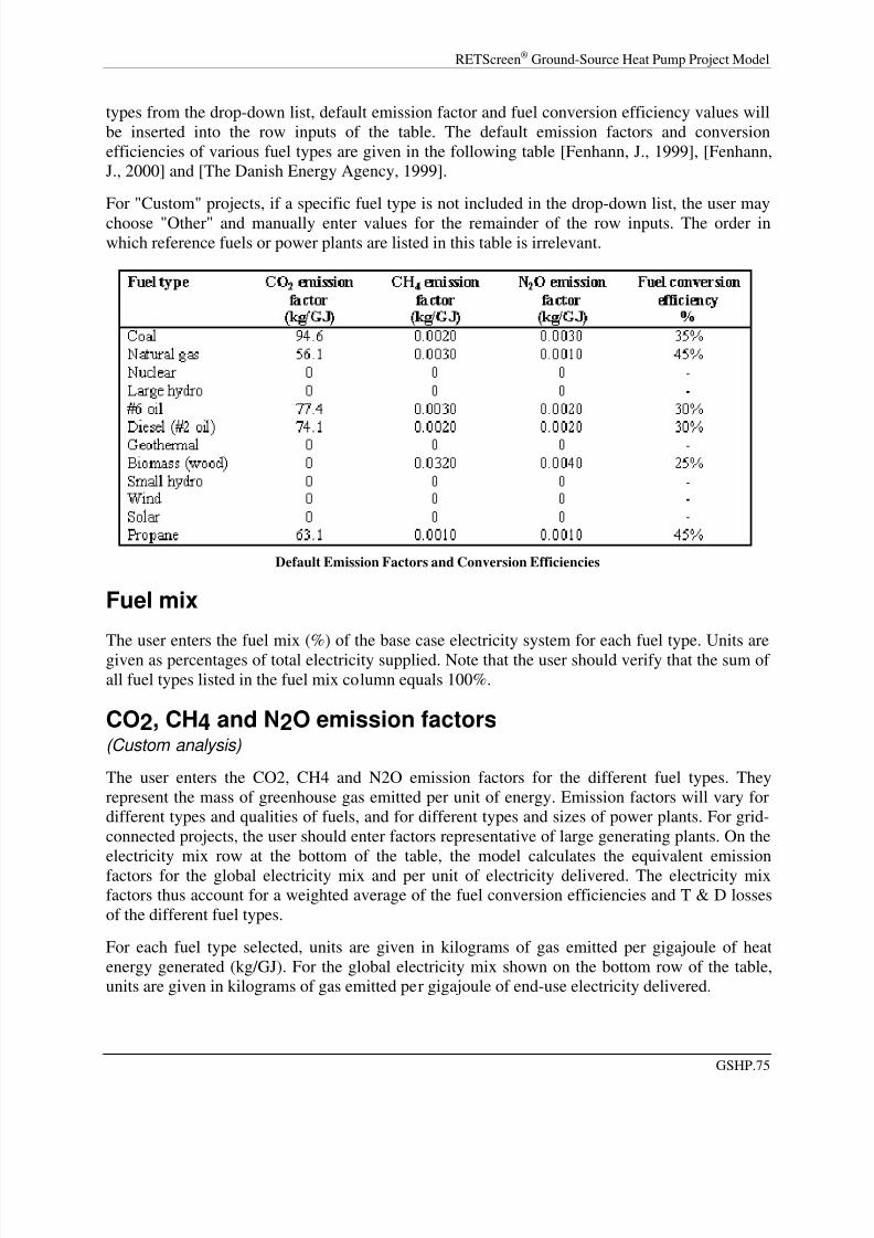
8/3/2019 GSHP3
http://slidepdf.com/reader/full/gshp3 75/104
RETScreen® Ground-Source Heat Pump Project Model
types from the drop-down list, default emission factor and fuel conversion efficiency values willbe inserted into the row inputs of the table. The default emission factors and conversionefficiencies of various fuel types are given in the following table [Fenhann, J., 1999], [Fenhann,J., 2000] and [The Danish Energy Agency, 1999].
For "Custom" projects, if a specific fuel type is not included in the drop-down list, the user may
choose "Other" and manually enter values for the remainder of the row inputs. The order inwhich reference fuels or power plants are listed in this table is irrelevant.
Default Emission Factors and Conversion Efficiencies
Fuel mix
The user enters the fuel mix (%) of the base case electricity system for each fuel type. Units aregiven as percentages of total electricity supplied. Note that the user should verify that the sum of all fuel types listed in the fuel mix column equals 100%.
CO2, CH4 and N2O emission factors(Custom analysis)
The user enters the CO2, CH4 and N2O emission factors for the different fuel types. Theyrepresent the mass of greenhouse gas emitted per unit of energy. Emission factors will vary fordifferent types and qualities of fuels, and for different types and sizes of power plants. For grid-connected projects, the user should enter factors representative of large generating plants. On theelectricity mix row at the bottom of the table, the model calculates the equivalent emissionfactors for the global electricity mix and per unit of electricity delivered. The electricity mixfactors thus account for a weighted average of the fuel conversion efficiencies and T & D lossesof the different fuel types.
For each fuel type selected, units are given in kilograms of gas emitted per gigajoule of heatenergy generated (kg/GJ). For the global electricity mix shown on the bottom row of the table,units are given in kilograms of gas emitted per gigajoule of end-use electricity delivered.
GSHP.75

8/3/2019 GSHP3
http://slidepdf.com/reader/full/gshp3 76/104
RETScreen® Software Online User Manual
For more information on determining GHG emission factors, see the revised IPCC Guidelinesfor National Greenhouse Gas Inventories. CO2 emission factors for many fuels are included onpage 1.13 of the IPCC Reference Manual. CH4 and N2O emission factors for a number of fuelsare included on pages 1.35 and 1.36 of the IPCC Reference Manual.
CO2, CH4 and N2O emission factors(Standard analysis)
The model provides the CO2, CH4 and N2O emission factors which represent the mass of greenhouse gas emitted per unit of energy. Emission factors will vary for different types andqualities of fuels, and for different types and sizes of power plants. The default factors providedare those which are representative of large power plants that feed a central electricity grid. Onthe electricity mix row at the bottom of the table, the model calculates the equivalent emissionfactors for the total electricity mix and per unit of electricity delivered. The electricity mixfactors thus account for a weighted average of the fuel conversion efficiencies and T & D lossesof the different fuel types.
For each fuel type selected, units are given in kilograms of gas emitted per gigajoule of heatenergy generated (kg/GJ). For the total electricity mix shown on the bottom row of the table,units are given in kilograms of gas emitted per gigajoule of end-use electricity delivered.
For more information on determining GHG emission factors, see the revised IPCC Guidelinesfor National Greenhouse Gas Inventories. CO2 emission factors for many fuels are included onpage 1.13 of the IPCC Reference Manual. CH4 and N2O emission factors for a number of fuelsare included on pages 1.35 and 1.36 of the IPCC Reference Manual.
The default values provided by the model are given in the Default Emission Factors andConversion Efficiencies table.
Fuel conversion efficiency(Custom analysis)
The user enters the fuel conversion efficiency for the selected fuel type. The fuel conversionefficiency is the efficiency of energy conversion from primary heat potential to actual powerplant output. This value is used to calculate, for each fuel type, the aggregate GHG emissionfactor and therefore is only relevant for fuel types which actually produce greenhouse gases (i.e.with non-zero CO2, CH4 and N2O emission factors).
For example, a typical coal-fired power plant could have a fuel conversion efficiency of 35%,which indicates that 35% of the heat content of the coal is transformed into electricity fed to the
grid.
Units are given as a percentage of primary heat potential (gigajoules of heat) to actual powerplant output (gigajoules of electricity). Fuel types which emit no GHGs (e.g. solar) have a defaultvalue of 100%.
GSHP.76

8/3/2019 GSHP3
http://slidepdf.com/reader/full/gshp3 77/104
RETScreen® Ground-Source Heat Pump Project Model
Fuel conversion efficiency(Standard analysis)
The model provides the fuel conversion efficiency for the selected fuel type. The fuel conversionefficiency is the efficiency of energy conversion from primary heat potential to actual power
plant output. This value is used to calculate, for each fuel type, the aggregate GHG emissionfactor and therefore is only relevant for fuel types which actually produce greenhouse gases (i.e.with non-zero CO2, CH4 and N2O emission factors).
For example, a typical coal-fired power plant could have a fuel conversion efficiency of 35%,which indicates that 35% of the heat content of the coal is transformed into electricity fed to thegrid.
Units are given as a percentage of primary heat potential (gigajoules of heat) to actual powerplant output (gigajoules of electricity). Fuel types which emit no GHGs (e.g. solar) have a defaultvalue of 100%.
The default values provided by the model are given in the Default Emission Factors andConversion Efficiencies table.
Transmission and distribution losses
The user enters the transmission and distribution (T & D) losses (%) of the base case electricitysystem, which includes all energy losses between the power plant and the end-user. This valuewill vary based on the voltage of transport lines, the distance from the site of energy productionto the point of use, peak energy demands, ambient temperature and electricity theft. In addition,T & D system type (e.g. AC vs. DC) and quality may also influence losses. The model calculatesthe weighted average of the T & D losses of the global electricity mix on the bottom row of thetable.
Units are given as a percentage of all electricity losses to electricity generated. It is reasonable toassume T & D losses of 8 to 10% in modern grids in industrialised countries and 10 to 20% ingrids located in developing countries.
GHG emission factor
The model calculates the GHG emission factor for each reference fuel type. Values arecalculated based on the individual emission factors, the fuel conversion efficiency and the T & Dlosses. The weighted GHG emission factor for the total electricity mix is calculated on thebottom row of the table.
Units are given in tonnes equivalent of CO2 emission per megawatt-hour of end-use electricity
delivered (tCO2 /MWh).
GSHP.77

8/3/2019 GSHP3
http://slidepdf.com/reader/full/gshp3 78/104
RETScreen® Software Online User Manual
Base Case Heating and Cooling System (Baseline)
The base case heating and cooling system, or baseline system, represents the system to which theground-source heat pump is compared. The base case heating and cooling system is defined interms of its fuel types, its emissions of GHG and its conversion efficiencies.
Note that in all cases, the base cooling system is assumed to be powered by electricity using thebase case electricity mix system.
The base case system is normally referred to as the reference or baseline option in standardeconomic analysis.
Fuel type
The fuel type of the base case heating system entered by the user in the Energy Model worksheetis transferred to the GHG Analysis worksheet.
The fuel type of the base case cooling system is assumed to be powered by electricity in allcases.
Fuel mix
The base case heating and cooling systems are assumed to be fuelled by a single source of energy and the fuel mix is therefore set to 100%.
CO2, CH4 and N2O emission factors(Custom analysis)
For the base case heating system, the user enters the CO2, CH4 and N2O emission factorscorresponding to the heating fuel type selected. If the heating fuel type is electricity, emissionfactors of the base case electricity mix are used. For the base case cooling system, CO2, CH4 andN2O emission factors for the base case electricity mix are used.
CO2, CH4 and N2O emission factors represent the mass of greenhouse gas emitted per unit of energy generated. Emission factors will vary for different types and qualities of fuels, and fordifferent types and sizes of heating equipment.
For each fuel type selected, units are given in kilograms of gas emitted per gigajoule of heatingor cooling energy generated (kg/GJ).
For more information on determining GHG emission factors, see the revised IPCC Guidelinesfor National Greenhouse Gas Inventories. CO2 emission factors for many fuels are included on
page 1.13 of the IPCC Reference Manual. CH4 and N2O emission factors for a number of fuels
are included on pages 1.35 and 1.36 of the IPCC Reference Manual.
GSHP.78

8/3/2019 GSHP3
http://slidepdf.com/reader/full/gshp3 79/104
RETScreen® Ground-Source Heat Pump Project Model
CO2, CH4 and N2O emission factors(Standard analysis)
For the base case heating system, the model provides the CO2, CH4 and N2O emission factorscorresponding to the heating fuel type selected. If the heating fuel type is electricity, emission
factors of the base case electricity mix are used. For the base case cooling system, CO2, CH4 andN2O emission factors for the base case electricity mix are used.
CO2, CH4 and N2O emission factors represent the mass of greenhouse gas emitted per unit of energy generated. Emission factors will vary for different types and qualities of fuels, and fordifferent types and sizes of heating equipment. The default factors provided are those which arerepresentative of large heating plants. For smaller plants and for greater accuracy, the user mayselect the "Custom" type of analysis and specify the emission factors.
For each fuel type selected, units are given in kilograms of gas emitted per gigajoule of primaryheating or cooling energy generated (kg/GJ).
For more information on determining GHG emission factors, see the revised IPCC Guidelinesfor National Greenhouse Gas Inventories. CO2 emission factors for many fuels are included on
page 1.13 of the IPCC Reference Manual. CH4 and N2O emission factors for a number of fuels
are included on pages 1.35 and 1.36 of the IPCC Reference Manual.
The default values provided by the model are given in the Default Emission Factors andConversion Efficiencies table.
Fuel conversion efficiency
The base case heating and cooling system fuel conversion efficiencies are entered by the user in
the Energy Model worksheet and are transferred to the GHG Analysis worksheet. The fuelconversion efficiency represents the annual average efficiency of energy conversion fromprimary heat potential to actual heating, or cooling, energy output. This value is used tocalculate, for each fuel type, the aggregate GHG emission factor and therefore is only relevantfor fuel types which actually produce greenhouse gases (i.e. with non-zero CO2, CH4 and N2Oemission factors).
Units are given as a percentage of actual space heating and cooling energy output (gigajoules of heating/cooling energy) to primary heat potential (gigajoules of heat or electricity).
GHG emission factor
The model calculates the GHG emission factor for the base case heating and cooling systems.Values are calculated based on the individual emission factors and the fuel conversion efficiency.
Units are given in tonnes equivalent of CO2 emission per megawatt-hour of end-use space
heating and cooling energy delivered (tCO2 /MWh).
GSHP.79

8/3/2019 GSHP3
http://slidepdf.com/reader/full/gshp3 80/104
RETScreen® Software Online User Manual
Proposed Case Heating and Cooling System (Ground-SourceHeat Pump)
The proposed case heating and cooling system, or mitigation system, is the proposed project. It isdefined in terms of its fuel types, its emissions of GHG and its conversion efficiencies. Note thatin all cases, the ground-source heat pump is assumed to be electricity-driven using the base caseelectricity system.
The proposed case system is normally referred to as the mitigation option in standard economicanalysis.
Fuel type
The fuel type of the ground-source heat pump is assumed to be electricity for both heating andcooling.
Fuel mix
The fuel mix of the ground-source heat pump is assumed to come from a single source,i.e. electricity, and is thus set to 100%.
CO2, CH4 and N2O emission factors
The model provides the CO2, CH4 and N2O emission factors corresponding to the fuel type,i.e. electricity used to drive the ground-source heat pump. These values correspond to theelectricity mix of the base case electricity system.
For each fuel type selected, units are given in kilograms of gas emitted per gigajoule of electricity used by the ground-source heat pump in both the heating and cooling mode (kg/GJ).
Fuel conversion efficiency
The model calculates the fuel conversion efficiency in the Energy Model worksheet and thevalue is transferred to the GHG Analysis worksheet. The fuel conversion heating and coolingefficiencies are equivalent to the "Seasonal heating COP" and the "Seasonal cooling COP"respectively, as they appear in the Energy Model worksheet.
The fuel conversion efficiency represents the annual average efficiency of energy conversionfrom electricity to actual space heating and cooling energy output. This value is used inconjunction with the CO2, CH4 and N2O emission factors to calculate the aggregate GHGemission factor for the proposed project.
Units are given as a percentage of actual space heating or cooling energy output (gigajoules of heating/cooling energy) to electricity input (gigajoules of electricity).
GSHP.80

8/3/2019 GSHP3
http://slidepdf.com/reader/full/gshp3 81/104
RETScreen® Ground-Source Heat Pump Project Model
GHG emission factor
The model calculates the GHG emission factor for the proposed ground-source heat pumpsystem. Values are calculated based on the individual CO2, CH4 and N2O emission factors andthe fuel conversion efficiency.
Units are given in tonnes equivalent of CO2 emission per megawatt-hour of end-use spaceheating and cooling energy delivered (tCO2 /MWh).
GHG Emission Reduction Summary
Based on the GHG emission data entered, the model calculates the annual reduction in GHGemissions when the base case system is displaced with the proposed case system.
Base case GHG emission factor
The model transfers the base case GHG emission factor calculated in the base case heating andcooling system (baseline) section. This value represents the amount of GHG emitted per unit of space heating and cooling energy delivered for the base case system. The GHG emission factorfor the base case cooling system is assumed to be zero in cases with no air-conditioning.
Units are given in tonnes equivalent of CO2 emission per megawatt-hour of space heating and
cooling energy delivered (tCO2 /MWh).
Proposed case GHG emission factor
The model transfers the proposed case GHG emission factor calculated in the proposed case
heating and cooling system section. This value represents the amount of GHG emitted per unit of space heating and cooling energy delivered if the ground-source heat pump is installed.
Units are given in tonnes equivalent of CO2 emission per megawatt-hour of space heating and
cooling energy delivered (tCO2 /MWh).
End-use annual energy delivered
The model displays the end-use annual energy delivered, as calculated in the Energy Model worksheet.
Units are given in megawatt-hours of space heating and cooling energy delivered (MWh).
GSHP.81

8/3/2019 GSHP3
http://slidepdf.com/reader/full/gshp3 82/104
RETScreen® Software Online User Manual
Annual GHG emission reduction
The model calculates the annual reduction in GHG emissions estimated to occur if the proposedproject is implemented. The calculation is based on emission factors of both the base case andthe proposed case system and on the end-use annual energy delivered.
Units are given in equivalent tonnes of CO2 emission per year (tCO2 /yr).
Note: At this point, the user should complete the Financial Summary worksheet.
GSHP.82

8/3/2019 GSHP3
http://slidepdf.com/reader/full/gshp3 83/104
RETScreen® Ground-Source Heat Pump Project Model
Sensitivity and Risk Analysis
As part of the RETScreen Clean Energy Project Analysis Software, a Sensitivity and Risk
Analysis worksheet is provided to help the user estimate the sensitivity of important financialindicators in relation to key technical and financial parameters. This standard sensitivity and risk
analysis worksheet contains two main sections: Sensitivity Analysis and Risk Analysis. Eachsection provides information on the relationship between the key parameters and the importantfinancial indicators, showing the parameters which have the greatest impact on the financialindicators. The Sensitivity Analysis section is intended for general use, while the Risk Analysissection, which performs a Monte Carlo simulation, is intended for users with knowledge of statistics.
Both types of analysis are optional. Inputs entered in this worksheet will not affect results inother worksheets.
Use sensitivity analysis sheet?
The user indicates, by selecting from the drop-down list, whether or not the optional Sensitivity
and Risk Analysis worksheet is used to conduct a sensitivity analysis of the important financialindicators.
If the user selects "Yes" from the drop-down list, the sensitivity analysis section will open andthe user should complete the top part of the worksheet. The user will need to click on "CalculateSensitivity Analysis" button to get the results.
Perform risk analysis too?
The user indicates, by selecting from the drop-down list, whether or not the optional risk analysissection is used to conduct a risk analysis of the important financial indicators, in addition to thesensitivity analysis. In the risk analysis section, the impact of each input parameter on a financialindicator is obtained by applying a standardised multiple linear regression on the financialindicator.
If the user selects "Yes" from the drop-down list, then the risk analysis section will open and theuser should complete the lower-half of the worksheet. The analysis will be performed on thefinancial indicator selected by the user in the "Perform analysis on" input cell at the top-right.The user will need to click on "Calculate Risk Analysis" button in the Risk Analysis section atthe lower-half of this worksheet to get the results.
Project name
The user-defined project name is entered for reference purposes only in the Energy Model
worksheet, and it is copied automatically to the Sensitivity worksheet.
GSHP.83
8/3/2019 GSHP3
http://slidepdf.com/reader/full/gshp3 84/104
RETScreen® Software Online User Manual
Project location
The user-defined project location is entered for reference purposes only in the Energy Model
worksheet, and it is copied automatically to the Sensitivity worksheet.
Perform analysis on
The user selects, from three options in the drop-down list, the financial indicator to be used forboth the sensitivity and risk analyses. Modifying the selection in this cell will change the resultsin the worksheet.
After-tax Internal Rate of Return and Return on Investment
The model calculates the after-tax internal rate of return (%), which represents the true interestyield provided by the project equity over its life. It is also referred to as the return on investment(equity) (ROI) or the time-adjusted rate of return. It is calculated by finding the discount rate that
causes the net present value of the project to be equal to zero. Hence, it is not necessary toestablish the discount rate of an organisation to use this indicator. An organisation interested in aproject can compare the internal rate of return of the project to its required rate of return (often,the cost of capital). The IRR is calculated on a nominal basis, that is including inflation.
If the internal rate of return of the project is equal to or greater than the required rate of return of the organisation, then the project will likely be considered financially acceptable (assumingequal risk). If it is less than the required rate of return, the project is typically rejected. Anorganisation may have multiple required rates of return that will vary according to the perceivedrisk of the projects. The most obvious advantage of using the internal rate of return indicator toevaluate a project is that the outcome does not depend on a discount rate that is specific to agiven organisation. Instead, the IRR obtained is specific to the project and applies to all investorsin the project. The model uses the after-tax yearly cash flows and the project life to calculate theinternal rate of return.
Year-to-positive cash flow
The model calculates the number of years to positive (cumulative) cash flow, which representsthe length of time that it takes for the owner of a project to recoup its own initial investment outof the project cash flows generated. The year-to-positive cash flow considers project cash flowsfollowing the first year as well as the leverage (level of debt) of the project, which makes it abetter time indicator of the project merits than the simple payback. The model uses the yearnumber and the cumulative after-tax cash flows in order to calculate this value.
The year-to-positive cash flow differs from the discounted payback indicator in that it considersthe nominal value of future cash flows rather than the discounted value of future cash flows.
Net Present Value - NPV
The model calculates the net present value (NPV) of the project, which is the value of all futurecash flows, discounted at the discount rate, in today's currency. NPV is thus calculated at a time
GSHP.84

8/3/2019 GSHP3
http://slidepdf.com/reader/full/gshp3 85/104
RETScreen® Ground-Source Heat Pump Project Model
0 corresponding to the junction of the end of year 0 and the beginning of year 1. Under the NPVmethod, the present value of all cash inflows is compared against the present value of all cashoutflows associated with an investment project. The difference between the present value of these cash flows, called the NPV, determines whether or not the project is generally a financiallyacceptable investment. Positive NPV values are an indicator of a potentially feasible project. In
using the net present value method, it is necessary to choose a rate for discounting cash flows topresent value. As a practical matter, organisations put much time and study into the choice of adiscount rate. The model calculates the NPV using the cumulative after-tax cash flows. In caseswhere the user has selected not to conduct a tax analysis, the NPV calculated will be that of thepre-tax cash flows.
Sensitivity range
The user enters the sensitivity range (%), which defines the maximum percentage variation thatwill be applied to all the key parameters in the sensitivity analysis results tables. Each parameteris varied by the following fraction of the sensitivity range : -1, -1/2, 0, 1/2, 1. This value is used
in the sensitivity analysis section only.The sensitivity range entered by the user must be a percentage value between 0 and 50%.
Threshold
The user enters the threshold value for the financial indicator selected. The threshold is the valueunder which (for the "After tax IRR and ROI" and "Net Present Value - NPV") or over which(for "Year-to-positive cash flow") the user considers that the proposed project is not financiallyviable. Results which indicate an unviable project, as defined by the user threshold, will appearas orange cells in the sensitivity analysis results tables. This value is used in the sensitivityanalysis section only.
Click here to Calculate Sensitivity Analysis
The "Click here to Calculate Sensitivity Analysis" button updates the sensitivity analysiscalculations using the input parameters specified by the user (i.e. "Perform analysis on" and"Sensitivity range" input cells). The sensitivity analysis tables are updated each time the userclicks on this button.
The sensitivity analysis calculations can take up to 15 seconds to run depending on the Excelversion and the speed of the computer. When the sensitivity analysis is updated, the buttondisappears.
If the user makes any changes to the input parameters, or navigates through any of the otherworksheets, the button will reappear. The user will then have to click on the button to update thesensitivity analysis calculations so that the results reflect the changes.
GSHP.85

8/3/2019 GSHP3
http://slidepdf.com/reader/full/gshp3 86/104
RETScreen® Software Online User Manual
Sensitivity Analysis for...
This section presents the results of the sensitivity analysis. Each table shows what happens to theselected financial indicator (e.g. After-tax IRR and ROI) when two key parameters (e.g. Initialcosts and Avoided cost of heating energy) are varied by the indicated percentages. Parameters
are varied using the following fraction of the sensitivity range : -1, -1/2, 0, 1/2, 1. Original values(which appear in the Financial Summary worksheet) are in bold in these sensitivity analysisresults tables.
Results which indicate an unviable project, as defined by the user threshold, will appear asorange cells in these sensitivity analysis results tables.
All parameter values used for the calculations are taken from the Financial Summary worksheetand all the sensitivity variations are evaluated at the level of that worksheet. This is a partiallimitation of this sensitivity analysis worksheet since some parameter values are calculated frominputs in other worksheets, but those inputs are not changed. However, for most cases, thislimitation is without consequence. If required, the user can use the blank worksheets (Sheet1,
etc.) to perform a more detailed analysis.
Risk Analysis for...
This section allows the user to perform a Risk Analysis by specifying the uncertainty associatedwith a number of key input parameters and to evaluate the impact of this uncertainty on after-taxIRR and ROI, year-to-positive cash flow or net present value (NPV).
The risk analysis is performed using a Monte Carlo simulation that includes 500 possiblecombinations of input variables resulting in 500 values of after-tax IRR and ROI, year-to-positive cash flow or net present value (NPV). The risk analysis allows the user to assess if the
variability of the financial indicator is acceptable, or not, by looking at the distribution of thepossible outcomes. An unacceptable variability will be an indication of a need to put more effortinto reducing the uncertainty associated with the input parameters that were identified as havingthe greatest impact on the financial indicator.
Avoided cost of heating energy
The avoided cost of heating energy is automatically transferred from the Financial Summary worksheet to the Sensitivity worksheet.
The user enters the avoided cost of energy range. The range is a percentage corresponding to theuncertainty associated with the estimated avoided cost of heating energy value. The higher thepercentage, the greater the uncertainty. The range specified by the user must be between 0 and50%. The range determines the limits of the interval of possible values that the avoided cost of heating energy could take.
For example, a range of 10% for an avoided cost of heating energy of $0.09/kWh means that theavoided cost of heating energy could take any value between $0081/kWh and $0.099/kWh. Since$0.09/kWh is the estimated value, the risk analysis will consider this value as being the most
GSHP.86
8/3/2019 GSHP3
http://slidepdf.com/reader/full/gshp3 87/104
RETScreen® Ground-Source Heat Pump Project Model
probable and the minimum and maximum values as being the least probable, based on a normaldistribution.
If the avoided cost of heating energy is known exactly by the user (no uncertainty), the usershould enter a range of 0%.
Initial costs
The total initial cost is transferred automatically from the Financial Summary worksheet to theSensitivity worksheet.
The user enters the initial costs range. The range is a percentage corresponding to the uncertaintyassociated with the estimated initial costs value. The higher the percentage, the greater theuncertainty. The range specified by the user must be between 0 and 50%. The range determinesthe limits of the interval of possible values that the initial costs could take.
For example, a range of 10% for initial costs of $30,000 means that the initial costs could take
any value between $27,000 and $33,000. Since $30,000 is the estimated value, the risk analysiswill consider this value as being the most probable and the minimum and maximum values asbeing the least probable, based on a normal distribution.
If the initial costs are known exactly by the user (no uncertainty), the user should enter a rangeof 0%.
Annual costs
The annual cost is transferred automatically from the Financial Summary worksheet to theSensitivity worksheet, but does not include debt payments.
The user enters the annual cost range. The range is a percentage corresponding to the uncertaintyassociated with the estimated annual costs value. The higher the percentage, the greater theuncertainty. The range specified by the user must be between 0 and 50%. The range determinesthe limits of the interval of possible values that the annual costs could take.
For example, a range of 10% for an annual cost of $800 means that the annual cost could takeany value between $720 and $880. Since $800 is the estimated value, the risk analysis willconsider this value as being the most probable and the minimum and maximum values as beingthe least probable, based on a normal distribution.
If the annual costs are known exactly by the user (no uncertainty), the user should enter a rangeof 0%.
Debt ratio
The debt ratio is automatically transferred from the Financial Summary worksheet to theSensitivity worksheet.
The user enters the debt ratio range. The range is a percentage corresponding to the uncertaintyassociated with the estimated debt ratio value. The higher the percentage, the greater the
GSHP.87

8/3/2019 GSHP3
http://slidepdf.com/reader/full/gshp3 88/104
RETScreen® Software Online User Manual
uncertainty. The range specified by the user must be a percentage value between 0% and thelowest percentage such that the debt ratio will always fall between 0 and 100%. The rangedetermines the limits of the interval of possible values that the debt ratio could take.
For example, a range of 10% for a debt ratio of 70% means that the debt ratio could take anyvalue between 63 and 77%. Since 70% is the estimated value, the risk analysis will consider this
value as being the most probable and the minimum and maximum values as being the leastprobable, based on a normal distribution.
If the debt ratio is known exactly by the user (no uncertainty), the user should enter a rangeof 0%.
Debt interest rate
The debt interest rate is automatically transferred from the Financial Summary worksheet to theSensitivity worksheet.
The user enters the debt interest rate range. The range is a percentage corresponding to theuncertainty associated with the estimated debt interest rate value. The higher the percentage, thegreater the uncertainty. The range specified by the user must be between 0 and 50%. The rangedetermines the limits of the interval of possible values that the debt interest rate could take.
For example, a range of 10% for a debt interest rate of 20% means that the debt interest ratecould take any value between 18 and 22%. Since 20% is the estimated value, the risk analysiswill consider this value as being the most probable and the minimum and maximum values asbeing the least probable, based on a normal distribution.
If the debt interest rate is known exactly by the user (no uncertainty), the user should enter arange of 0%.
Debt term
The debt term is automatically transferred from the Financial Summary worksheet to theSensitivity worksheet.
The user enters the debt term range. The range is a percentage corresponding to the uncertaintyassociated with the estimated debt term value. The higher the percentage, the greater theuncertainty. The range specified by the user must be a percentage value between 0% and thelowest percentage such that the debt term will always fall between 1 year and the project life.The range determines the limits of the interval of possible values that the debt term could take.
For example, a range of 10% for a debt term of 20 years means that the debt term could take anyvalue between 18 and 22 years. Since 20 years is the estimated value, the risk analysis willconsider this value as being the most probable and the minimum and maximum values as beingthe least probable, based on a normal distribution.
If the debt term is known exactly by the user (no uncertainty), the user should enter a rangeof 0%.
GSHP.88

8/3/2019 GSHP3
http://slidepdf.com/reader/full/gshp3 89/104
RETScreen® Ground-Source Heat Pump Project Model
GHG emission reduction credit
The GHG emission reduction credit is automatically transferred from the Financial Summary worksheet to the Sensitivity worksheet.
The user enters the GHG emission reduction credit range. The range is a percentagecorresponding to the uncertainty associated with the estimated GHG emission reduction creditvalue. The higher the percentage, the greater the uncertainty. The range specified by the usermust be a percentage value between 0 and 50%. The range determines the limits of the intervalof possible values that the GHG emission reduction credit could take.
For example, a range of 10% for a GHG emission reduction credit of $5/t CO2 means that the
GHG emission reduction credit could take any value between $4.5/tCO2 and $5.5/tCO2. Since
$5/tCO2 is the estimated value, the risk analysis will consider this value as being the most
probable and the minimum and maximum values as being the least probable, based on a normaldistribution.
If the GHG emission reduction credit is known exactly by the user (no uncertainty), the usershould enter a range of 0%.
Click here to Calculate Risk Analysis
The "Click here to Calculate Risk Analysis" button updates the risk analysis calculations usingthe input parameter ranges specified by the user. Clicking on this button starts a Monte Carlosimulation that uses 500 possible combinations of input variables resulting in 500 values of theselected financial indicator. The impact graph, the median, the minimum and maximumconfidence levels, and the distribution graph are calculated using these results and updated eachtime the user clicks on the button "Click here to Calculate Risk Analysis."
The risk analysis calculations can take up to 1 minute to run depending on the Excel version andthe speed of the computer. When the risk analysis is updated, the button disappears.
If the user makes any changes to the input range values, or navigates through any of the otherworksheets, the button will reappear. The user will then have to click on the button to update therisk analysis calculations so that the results reflect the changes.
Impact graph
The impact graph shows the relative contribution of the uncertainty in each key parameter to thevariability of the financial indicator. The X axis at the bottom of the graph does not have anyunits, but rather presents a relative indication of the strength of the contribution of eachparameter.
The longer the horizontal bar, for a given input parameter, the greater is the impact of the inputparameter on the variability of the financial indicator.
The input parameters are automatically sorted by their impact on the financial indicator. Theinput parameter at the top (Y axis) contributes the most to the variability of the financial
GSHP.89

8/3/2019 GSHP3
http://slidepdf.com/reader/full/gshp3 90/104
RETScreen® Software Online User Manual
indicator while the input parameter at the bottom contributes the least. This "tornado graph" willhelp the user determine which input parameters should be considered for a more detailedanalysis, if that is required.
The direction of the horizontal bar (positive or negative) provides an indication of therelationship between the input parameter and the financial indicator. There is a positive
relationship between an input parameter and the financial indicator when an increase in the valueof that parameter results in an increase in the value of the financial indicator. For example, thereis usually a negative relationship between initial costs and the net present value (NPV), sincedecreasing the initial costs will increase the NPV.
In some cases, there is insufficient data to properly plot the graph. For example, when the year-to-positive cash flow is immediate, the result is not a numerical value, and therefore these valuescannot be plotted.
Median
The model calculates the median of the financial indicator. The median of the financial indicatoris the 50th percentile of the 500 values generated by the Monte Carlo simulation. The median willnormally be close to the financial indicator value calculated in the Financial Summary worksheet.
Level of risk
The user selects from the drop-down list the acceptable level of risk for the financial indicatorunder consideration. The options are: 5%, 10%, 15%, 20% and 25%.
The level of risk input is used to establish a confidence interval (defined by maximum and
minimum limits) within which the financial indicator is expected to fall. The level of risk represents the probability that the financial indicator will fall outside this confidence interval.
The limits of the confidence interval are automatically calculated based on the median and thelevel of risk, and are shown as "Minimum within level of confidence" and "Maximum withinlevel of confidence."
It is suggested that the user select a level of risk of 5 or 10%, which are typical values forstandard risk analysis.
Minimum within level of confidence
The model calculates the "Minimum within level of confidence," which is the lower limit of theconfidence interval within which the financial indicator likely falls. It is the percentile of thedistribution of the financial indicator corresponding to half the level of risk defined by the user.For example, for a "Minimum within level of confidence" value of 15% IRR, a level of risk of 10% means that 5% (half the level of risk) of the possible IRR values are lower than 15%.
GSHP.90

8/3/2019 GSHP3
http://slidepdf.com/reader/full/gshp3 91/104
RETScreen® Ground-Source Heat Pump Project Model
Maximum within level of confidence
The model calculates the "Maximum within level of confidence," which is the upper limit of theconfidence interval within which the financial indicator likely falls. It is the percentile of thedistribution of the financial indicator corresponding to 100% minus half the level of risk. For
example, for a "Maximum within level of confidence" value of 25% IRR, a level of risk of 10%means that 95% of the possible IRR values are lower than 25%.
Distribution graph
This histogram provides a distribution of the possible values for the financial indicator resultingfrom the Monte Carlo simulation. The height of each bar represents the frequency (%) of valuesthat fall in the range defined by the width of each bar. The value corresponding to the middle of each range is plotted on the X axis.
Looking at the distribution of financial indicator, the user is able to rapidly assess its' variability.
In some cases, there is insufficient data to properly plot the graph. For example, when the year-to-positive cash flow is immediate, the result is not a numerical value, and therefore these valuescannot be plotted.
Bar graph
The bar graph summarises the maximum and minimum financial indicator values that can beexpected according to the level of risk defined by the user.
GSHP.91

8/3/2019 GSHP3
http://slidepdf.com/reader/full/gshp3 92/104
RETScreen® Software Online User Manual
Product Data
Some of the product data requirements for the model are provided in the RETScreen OnlineProduct Database. To access the product database the user may refer to "Data & Help Access."
The product database provides information on the equipment associated with the project. From
the online product database dialogue box the user may obtain product specification andperformance data, as well as company contact information.
The product database sorting routine starts by using the "Design criteria" selected by the user inthe Energy Model worksheet. From the dialogue box the user selects the GSHP COP Range,followed by the Region, Supplier and Model. The data can be pasted from the dialogue box to thespreadsheets by clicking on the "Paste Data" button. Only data that are in bold are pasted to thespreadsheets; all other data are for reference purposes only. Data entered using the productdatabase may be overwritten, i.e. the user may prefer to use other data and can manually entervalues into the spreadsheets. "Other information" such as product weight and/or dimensions, isprovided to help the user prepare the study. The product database contains a link to the Websites
of some product suppliers. In the case where the Website link cannot be activated the user shouldtry using another browser or can contact the supplier by other means (email, fax, etc.).
Note: To see all the suppliers listed in the product database and their contact information, theuser can choose "Any" from the "GSHP COP Range" input cell.
The product database is distributed for informational purposes only and does not necessarilyreflect the views of the Government of Canada nor constitute an endorsement of any commercialproduct or person. Neither Canada nor its ministers, officers, employees or agents make anywarranty in respect to this database or assumes any liability arising out of this database.
Product manufacturers interested in having their products listed in the product database can reach
RETScreen
®
International at: RETScreen® InternationalCANMET Energy Technology Centre - VarennesNatural Resources Canada1615 Lionel-Boulet, P.O. Box 4800Varennes, Quebec, CANADA J3X 1S6Tel: +1-450-652-4621Fax: +1-450-652-5177E-mail: [email protected]
GSHP.92

8/3/2019 GSHP3
http://slidepdf.com/reader/full/gshp3 93/104
RETScreen® Ground-Source Heat Pump Project Model
Weather Data
This database includes some of the weather data required in the model. To access the weatherdatabase the user may refer to "Data & Help Access." While running the software the user may
obtain weather data from ground monitoring stations and/or from NASA's satellite data. Ground monitoring stations data is obtained by making a selection for a specific location fromthe Online Weather Database dialogue box. NASA's satellite data is obtained via a link toNASA's Website from the dialogue box.
Ground Monitoring Stations Data
From the dialogue box, the user selects a region, then a country, then a sub-region (provinces inCanada, states in the United States and N/A in the rest of the countries), and finally a weatherstation location. The weather station usually corresponds to the name of a city/town within theselected country. From the dialogue box the data can be pasted to the spreadsheets by clicking on
the "Paste Data" button. Only data that are in bold are pasted to the spreadsheets; all other dataare for reference purposes only. Data entered using the online weather database may beoverwritten; i.e. the user may prefer to use other data and can manually enter values into thespreadsheets. As an alternative the user can use the NASA satellite data, particularly for the casewhen the project location is not close to the given weather station location.
NASA Global Satellite Data
A link to the NASA Surface meteorology and Solar Energy Data Set Website is provided in theonline weather database dialogue box. The user is able to select the data required for the modelby clicking on a region on the world map illustrated on the NASA Website. The location is
narrowed down to a "cell" within a specified latitude and longitude. The user may simply copyand paste this data to the RETScreen spreadsheets or manually enter these values.
NASA and CETC - Varennes are co-operating to facilitate the use of NASA's global satellitesolar data with RETScreen and to develop a new global weather database (see Surfacemeteorology and Solar Energy Data Set for the tool). This work is sponsored as part of NASA'sEarth Science Enterprise Program and is being carried out at the NASA Langley Research Centerand at CETC - Varennes. This collaboration provides RETScreen users access (free-of-charge) tosatellite data (e.g. the amount of solar energy striking the surface of the earth, globaltemperatures and wind speeds), simply by clicking on links in either the RETScreen software orthe NASA Website. These data had previously only been available from a limited number of ground monitoring stations and are critical for assessing the amount of energy a project is
expected to produce. The use of these data results in substantial cost savings for users andincreased market opportunities for industry while allowing governments and industry to evaluateregional renewable energy resource potential.
GSHP.93

8/3/2019 GSHP3
http://slidepdf.com/reader/full/gshp3 94/104
RETScreen® Software Online User Manual
Cost Data
Typical cost data required to prepare RETScreen studies are provided in the RETScreen OnlineCost Database and in the Online Manual. This database is built into the "right-hand column" of the Cost Analysis worksheet. Data are provided for Canadian costs with 2000 as a baseline year.
The user also has the ability to create a custom cost database.
The user selects the reference (from the Cost Analysis worksheet) that will be used as a guidelinefor the estimation of costs associated with the implementation of the project. This feature allowsthe user to change the "Quantity Range" and the "Unit Cost Range" columns. The options fromthe drop-down list are: "Canada - 2000," "None," "Second currency" and a selection of 8 user-defined options ("Enter new 1," "Enter new 2," etc.).
If the user selects "Canada - 2000" the range of values reported in the "Quantity Range" and"Unit Cost Range" columns are for a 2000 baseline year, for projects in Canada and in Canadiandollars.
Selecting "None" hides the information presented in the "Quantity Range" and "Unit CostRange" columns. The user may choose this option, for example, to minimise the amount of information printed in the final report.
If the user selects "Second currency" two additional input cells appear in the next row: "Secondcurrency" and "Rate: 1st currency/2nd currency." In addition, the "Quantity Range" and "UnitCost Range" columns change to "% Foreign" and "Foreign Amount," respectively. This optionallows the user to assign a portion of a project cost item in a second currency, to account forthose costs that must be paid for in a currency other than the currency in which the project costsare reported. Note that this selection is for reference purposes only, and does not affect thecalculations made in other worksheets.
If "Enter new 1" (or any of the other 8 selections) is selected, the user may manually enterquantity and cost information that is specific to the region in which the project is located and/orfor a different cost base year. This selection thus allows the user to customise the information inthe "Quantity Range" and "Unit Cost Range" columns. The user can also overwrite "Enter new1" to enter a specific name (e.g. Japan - 2001) for a new set of unit cost and quantity ranges. Theuser may also evaluate a single project using different quantity and cost ranges; selecting a newrange reference ("Enter new 1" to "Enter new 8") enables the user to keep track of different costscenarios. Hence the user may retain a record of up to 8 different quantity and cost ranges thatcan be used in future RETScreen analyses and thus create a localised cost database.
GSHP.94

8/3/2019 GSHP3
http://slidepdf.com/reader/full/gshp3 95/104
RETScreen® Ground-Source Heat Pump Project Model
Training and Support
The user can obtain current information on RETScreen Training & Support at the following
Website address: www.retscreen.net/e/training/ .
GSHP.95

8/3/2019 GSHP3
http://slidepdf.com/reader/full/gshp3 96/104
RETScreen® Software Online User Manual
Term of Use
Disclaimer and Indemnification
RETScreen® International is provided on an "as is" basis. Natural Resources Canada nor does
its minister, officers, employees or agents make any representations or warranties, eitherexpressed or implied, arising by law or otherwise, including but not limited to, impliedwarranties of merchantability or fitness for a particular purpose, or that the use of the softwarewill not infringe any intellectual property rights of third parties. In no event will NaturalResources Canada nor its minister, officers, employees or agents have any obligations or liabilityarising from tort, or for loss of revenue or profit, or for indirect, special, incidental orconsequential damages as a result of your use of the software.
In consideration of the right to load, execute and use RETScreen® International, the recipient(Licensee) shall indemnify and save harmless Natural Resources Canada (Licensor), and itsemployees and agents, from and against, and shall be responsible for all claims, demands, losses,
costs, including solicitor and client costs, damages, actions suits or proceedings, arising out of,related to, or occasioned by any use of RETScreen International by the Licensee. The Licensorshall have the right to defend any such action or proceeding with counsel of its own selection.
Copyright and Trademark
The RETScreen® International Clean Energy Project Analysis Software and the accompanyingmanual and databases are copyright of the Minister of Natural Resources Canada (1997 - 2005).
Duplication in any manner is forbidden without prior written permission, which may be obtainedby contacting:
RETScreen® International
CANMET Energy Technology Centre - VarennesNatural Resources Canada1615 Lionel-Boulet, P.O. Box 4800Varennes, Quebec, CANADA J3X 1S6Tel: +1-450-652-4621Fax: +1-450-652-5177E-mail: [email protected] © Minister of Natural Resources Canada 1997 - 2005.RETSCREEN is a registered trademark of the Minister of Natural Resources Canada.
GSHP.96

8/3/2019 GSHP3
http://slidepdf.com/reader/full/gshp3 97/104
RETScreen® Ground-Source Heat Pump Project Model
License Agreement
The use of RETScreen® International is subject to the terms detailed in the RETScreenSoftware License Agreement, which is available at the following Website address:www.retscreen.net/license.html.
The user is encouraged to properly register at the RETScreen Website so that the Centre mayperiodically inform the user of product upgrades and be able to report on the global use of RETScreen.
GSHP.97

8/3/2019 GSHP3
http://slidepdf.com/reader/full/gshp3 98/104
RETScreen® Software Online User Manual
Bibliography
American Society of Heating, Refrigerating, and Air Conditioning Engineers (ASHRAE),ASHRAE Handbook, Fundamentals Volume, 1997.
American Society of Heating, Refrigerating, and Air Conditioning Engineers (ASHRAE),Commercial/Institutional Ground-Source Heat Pump Engineering Manual, 1995.
American Society of Heating, Refrigerating, and Air Conditioning Engineers (ASHRAE),ASHRAE Handbook, HVAC Systems and Equipment Volume, 1992.
American Society of Heating, Refrigerating, and Air Conditioning Engineers (ASHRAE),ASHRAE Handbook, Fundamentals Volume, 1985.
Chabot, B. "Personal Communication," 1999.
The Danish Energy Agency, Engerstatistics 1995, 1999.
Fenhann, J., "Personal Communication," January, 2000.
Fenhann, J., Projections of Emissions of Greenhouse Gases, Ozone precursors and SulphurDioxide from Danish Sources until 2010, The Danish Energy Agency, December 1999.
Leng, G., RETScreen International: A Decision-Support and Capacity-Building Tool forAssessing Potential Renewable Energy Projects, UNEP Industry & Environment, 3rd Quarter,2000.
Martinot, E. and McDoom, O., Promoting Energy Efficiency and Renewable Energy: GEFClimate Change Projects and Impacts, October 1999 Pre-Publication Draft, Global EnvironmentFacility, 1999.
McRae, S.G., Practical Pedology: Studying Soils in the Field, Halstead Press, New York, 1988.
Means, R.S., Mechanical Cost Data, 21st Annual Edition, R.S. Means Company Inc., KingstonMA, 1998.
Sandor, R., Walsh, M. and Leblanc, A., Creating a Market for Carbon Emissions: Gas IndustryOpportunities, published in Natural Gas , June 1999.
GSHP.98

8/3/2019 GSHP3
http://slidepdf.com/reader/full/gshp3 99/104
RETScreen® Ground-Source Heat Pump Project Model
Index
A
After-tax ................................................67, 71, 84, 86After-tax IRR and ROI ............................................86Air-conditioner seasonal COP .......... ............ ...........13Annual cooling energy demand...............................30Annual costs ................................................70, 71, 87Annual Costs (Credits) ............................................52Annual Costs and Debt............................................65Annual earth temperature amplitude........................25Annual Energy Balance ...........................................56Annual Energy Production ......................................20Annual GHG emission reduction.............................82Annual heating energy demand .......... ........... ..........32Annual Life Cycle Savings......................................69Annual Savings or Income.......................................66
Available information........................................25, 27Available land area..................................................10Average heat pump efficiency...............16, 17, 20, 21Average summer daily temperature range........... ....24Avoided cost of heating energy........... ........... ...58, 86
B
Background Information....................................72, 73Balance of System .............................................50, 64Bar graph.................................................................91Base Case Electricity System (Baseline)............... ..73
Base case GHG emission factor ..............................81Base Case Heating and Cooling System (Baseline) 78Base Case HVAC System........................................11Benefit-Cost (B-C) ratio .......... ........... ........... ..........69Bibliography............................................................98Blank Worksheets (3) ..........................................9, 55Brief Description and Model Flow Chart ............ ......4Building cooling energy demand.............................32Building design cooling load...................................31Building design heating load .......... ........... ........... ...30Building floor area...................................................27Building has air-conditioning? ........... ............ .........11Building Heating and Cooling Load........................26
Building heating energy demand.............................31
C
Calculate GHG reduction cost? ............ ........... ........69Cell Colour Coding....................................................5Circulating fluid.......................................................47Circulating pumps....................................................47Click here to Calculate Risk Analysis ............ .........89
Click here to Calculate Sensitivity Analysis............85CO2, CH4 and N2O emission factors...75, 76, 77, 78,
79, 80, 81Construction supervision .......... ........... ........... .........45Contingencies ....................................................52, 53Cooling . 11, 14, 17, 18, 19, 21, 23, 24, 25, 27, 30, 31,
32, 33, 57, 66, 72Cooling design temperature.........................23, 25, 31Cooling energy delivered.........................................57Cooling energy savings/income...............................66Cooling humidity level............................................24Copyright and Trademark........................................96Cost Analysis.. 6, 9, 20, 21, 22, 34, 36, 37, 47, 48, 49,
56, 57, 59, 61, 63, 64, 65, 66, 67, 94Cost Data ...........................................................94, 98Cost references ..............................................6, 37, 38Cumulative .......................................................56, 71
Cumulative Cash Flows Graph..........................56, 71Currency ........................................................6, 36, 38Currency Options.......................................................6Custom.......................................73, 74, 75, 76, 78, 79
D
Data & Help Access ................................5, 10, 92, 93Debt interest rate................................................60, 88Debt payments ...................................................65, 70Debt payments - debt term.......................................65Debt ratio...........................................................60, 87
Debt service coverage..............................................70Debt term...........................................................61, 88Demand charge ........................................................59Depreciation method................................................62Depreciation period .................................................63Depreciation rate......................................................63Depreciation tax basis..............................................62Depth of measurement of earth temperature............26Design cooling load...........................................11, 33Design criteria .......................................14, 18, 19, 92Design heating load ...........................................11, 32Detailed cost estimate..............................................41Development..........................................35, 42, 45, 64Disclaimer and Indemnification .......... ............ ........96Discount rate............................................................60Distribution graph....................................................91Drilling and grouting ...............................................48
E
Effective income tax rate.........................................61Electricity ..................................20, 21, 54, 57, 72, 74
GSHP.99

8/3/2019 GSHP3
http://slidepdf.com/reader/full/gshp3 100/104
RETScreen® Software Online User Manual
Electricity required ..................................................57Electricity used ..................................................20, 21End of project life ........................................55, 62, 67End of project life - Cost/Credit ........... ........... ........67End-use annual energy delivered.............................81Energy cost escalation rate ........... ........... ........... .....59Energy equipment....................................................64Energy Equipment...................................................46Energy Model9, 10, 11, 23, 30, 32, 46, 48, 49, 51, 54,
56, 57, 58, 73, 78, 79, 80, 81, 83, 84, 92Engineering............................................41, 44, 64, 98Equipment and lighting usage .................................29
F
Feasibility study.................................................39, 64Feasibility Study................................................39, 64Financial Feasibility ..........................................56, 67Financial Parameters..........................................56, 58
Financial Summary...9, 56, 58, 63, 71, 72, 73, 82, 86,87, 88, 89, 90
Fittings and valves ...................................................50Foreign Amount.....................................37, 38, 39, 94Foundation type.......................................................30Fuel conversion efficiency.....................76, 77, 79, 80Fuel mix.......................................................75, 78, 80Fuel type..........................................74, 76, 77, 78, 80Fuel/Electricity ..................................................54, 65
G
GHG credit escalation rate...........................58, 59, 66GHG emission factor...........72, 76, 77, 78, 79, 80, 81GHG emission reduction cost..................................69GHG emission reduction credit ....... 58, 59, 66, 69, 89GHG Emission Reduction Summary.................72, 81GHG reduction credit duration ........... ............ ...58, 59GHG reduction income - duration .......... ........... ......66Global Warming Potential of GHG.......... ............ ...73Greenhouse Gas Emission Reduction Analysis.........9Ground heat exchanger layout ........... ............ ..........14Ground Heat Exchanger System........................11, 13Ground HX loop pipes.............................................49Ground Monitoring Stations Data ...........................93Ground-Source Heat Pump Project Model........... .....9GSHP cooling energy delivered ..............................21GSHP heating energy delivered...............................21GSHP system design .........................................44, 45
H
Heat pump manufacturer .........................................17Heat pump model ....................................................17
Heat Pump System.............................................11, 16Heat pumps..............................................................46Heating ... 9, 11, 12, 14, 18, 19, 20, 21, 23, 25, 27, 30,
31, 32, 56, 57, 66, 72, 98Heating and Cooling Load Calculation .........9, 23, 25Heating design temperature........... ............ ..23, 25, 30Heating energy delivered.........................................56Heating energy savings/income...............................66Heating fuel displaced .............................................57Heating fuel type .....................................................12Heating system seasonal efficiency........... ........... ...12
I
Impact graph............................................................89Incentives/Grants.....................................................65Income tax analysis?................................................61Incremental electricity load .......... ........... ..........54, 57Inflation ...................................................................60
Initial costs...................................................63, 86, 87Initial Costs........................................................39, 61Insulation level ..................................................28, 29Internal piping and insulation ........... ........... ........... .51
L
Land survey .............................................................43Latitude of project location......................................25Level of risk.............................................................90License Agreement..................................................97Loss carryforward?..................................................61
M
Maximum well flow rate .........................................16Maximum within level of confidence................90, 91Mean earth temperature...........................................25Median.....................................................................90Minimum within level of confidence.......................90Miscellaneous....................................................52, 65Model Flow Chart......................................................4
N
NASA Global Satellite Data....................................93Nearest location for weather data .......... ............ ......23Net GHG emission reduction.............................57, 58Net GHG emission reduction - credit duration........58Net GHG emission reduction - project life..............58Net Present Value - NPV.............................69, 84, 85Number of supply wells required ............................16Numbers of floors....................................................28
GSHP.100

8/3/2019 GSHP3
http://slidepdf.com/reader/full/gshp3 101/104
RETScreen® Ground-Source Heat Pump Project Model
O
O&M .....................................................43, 52, 53, 65O&M labour ......................................................52, 53Occupancy type .......................................................29Other...... 12, 42, 44, 45, 46, 49, 50, 51, 53, 57, 75, 92
P
Perform analysis on .....................................83, 84, 85Perform risk analysis too? .......................................83Periodic Costs (Credits).....................................54, 66Permits and approvals..............................................43Plate heat exchangers...............................................48Preliminary design...................................................41Pre-tax ...............................................................67, 70Printing a File ............................................................8Product Data ............................5, 7, 10, 17, 34, 46, 92Project Costs and Savings..................................56, 63Project debt..............................................................70Project equity...........................................................70Project financing......................................................43Project life ...............................................................60Project location......................................10, 56, 73, 84Project management ................................................44Project name ..........................................10, 56, 73, 83Property taxes/Insurance..........................................53Proposed case GHG emission factor ........... ............81Proposed Case Heating and Cooling System
(Ground-Source Heat Pump) ..............................80Pumping depth.........................................................15
R
Rate
1st currency / 2nd currency............. 37, 94Report preparation ...................................................41Required groundwater flow rate ........... ........... ........16Retail price of electricity .......... .......... ........... ..........59
S
Saving a File..............................................................7
Seasonal cooling COP .......................................22, 80Seasonal cooling EER .............................................22Seasonal heating COP .......................................21, 80Second currency ......................................6, 37, 38, 94Sensitivity and Risk Analysis ............ ........... .......9, 83Sensitivity range......................................................85Simple Payback .......................................................68Site Conditions ........................................................23Site investigation ...............................................39, 40
Soil type...................................................................10Soil/hydrology assessment.......................................40Standard......... 6, 14, 16, 17, 28, 36, 38, 73, 76, 77, 79Standard cooling COP .............................................17Standard heating COP .............................................17Suggested supplemental heat rejection....................20Suggested supplemental heating capacity................19Supplemental energy delivered................................20Supplemental heat rejection...............................20, 51Supplemental Heating and Heat Rejection System 11,
19Supplemental heating system ..................................50System Characteristics.............................................11System type .............................................................13
T
Tax holiday available?.............................................63Tax holiday duration................................................63
Tenders and contracting...........................................45Threshold.................................................................85Total borehole length...............................................15Total loop length......................................................15Total standard cooling capacity........... ........... ...18, 19Total standard heating capacity .......... ........... ..........18Total trench length...................................................15Training .............................................................52, 95Training and Support ...............................................95Transmission and distribution losses .......... ........... ..77Travel and accommodation..............39, 42, 44, 52, 53Trenching and backfilling........................................48Type of analysis...........................................35, 73, 74
Type of building ......................................................26Typical land area required .......... .......... .......... ...10, 14
U
Units, Symbols & Prefixes ........................................7Use GHG analysis sheet?.........................................72Use sensitivity analysis sheet?.................................83
W
Weather Data.........................5, 10, 23, 24, 25, 26, 93Well pumps..............................................................47Wellbore depth ........................................................16Window area............................................................28
Y
Yearly Cash Flows.......................................56, 70, 71Year-to-positive cash flow...........................68, 84, 85
GSHP.101

8/3/2019 GSHP3
http://slidepdf.com/reader/full/gshp3 102/104
RETScreen® Software Online User Manual
Notes:
GSHP.102

8/3/2019 GSHP3
http://slidepdf.com/reader/full/gshp3 103/104

8/3/2019 GSHP3
http://slidepdf.com/reader/full/gshp3 104/104
www.retscreen.net