NoticeThe information contained in this document is subject to change without notice.
Agilent Technologies makes no warranty of any kind with regard to this material, including but not limited to, the implied warranties of merchantability and fitness for a particular purpose. Agilent Technologies shall not be liable for errors contained herein or for incidental or consequential damages in connection with the furnishing, performance, or use of this material.
Technology Licenses The hardware and/or software described in this document are furnished under a license and may be used or copied only in accordance with the terms of such license.
Restricted Rights LegendIf software is for use in the performance of a U.S. Government prime contract or subcontract, Software is delivered and licensed as “Commercial computer software” as defined in DFAR 252.227-7014 (June 1995), or as a “commercial item” as defined in FAR 2.101(a) or as “Restricted computer software” as defined in FAR 52.227-19 (June 1987) or any equivalent agency regulation or contract clause. Use, duplication or disclosure of Software is subject to Agilent Technologies’ standard commercial license terms, and non-DOD Departments and Agencies of the U.S. Government will receive no greater than Restricted Rights as defined in FAR 52.227-19(c)(1-2) (June 1987). U.S. Government users will receive no greater than Limited Rights as defined in FAR 52.227-14 (June 1987) or DFAR 252.227-7015 (b)(2) (November 1995), as applicable in any technical data.
2
Safety InformationThe following safety symbols are used throughout this manual. Familiarize yourself with the symbols and their meaning before operating this instrument.
WARNING Warning denotes a hazard. It calls attention to a procedure which, if not correctly performed or adhered to, could result in injury or loss of life. Do not proceed beyond a warning note until the indicated conditions are fully understood and met.
CAUTION Caution denotes a hazard. It calls attention to a procedure that, if not correctly performed or adhered to, could result in damage to or destruction of the instrument. Do not proceed beyond a caution sign until the indicated conditions are fully understood and met.
NOTE Note calls out special information for the user’s attention. It provides operational information or additional instructions of which the user should be aware.
Where to Find the Latest InformationDocumentation is updated periodically. For the latest information about Agilent Technologies spectrum analyzer, including firmware upgrades and application information, please visit the following Internet URL:
This chapter provides overall information on the Agilent N9071A GSM/EDGE Measurement Application, and describes GSM and EDGE measurements made by the application. Installation instructions for adding this option to your analyzer are provided in this section, if you purchased this option separately.
9
Introduction to GSM and EDGEWhat does the Agilent N9071A GSM/EDGE Measurement Application do?
What does the Agilent N9071A GSM/EDGE Measurement Application do?This application makes measurements that conform to the ETSI EN 300 910 (GSM 05.05), ETSI EN 300 607.1, (GSM 11.10-1), ETSI EN 301 087 (GSM 11.21), and ANSI J-STD-007 specifications. It also complies with the 3GPP TS 51.021 Base Station System (BSS) equipment specification; Radio Aspects (Release-5) V.5.3.0 (2003-06), and the 3GPP TS 51.010-1 Mobile Station (MS) Conformance specification; Part 1: Conformance specification (Release-5) V.5.4.0 (2003-06).
These documents define complex, multi-part measurements used to maintain an interference-free environment. For example, the documents include measuring the power of a carrier. The application automatically makes these measurements using the measurement methods and limits defined in the standards. The detailed results displayed by the measurements allow you to analyze GSM and EDGE system performance. You may alter the measurement parameters for specialized analysis.
This application was primarily developed for making measurements on digital transmission carriers. These measurements can help determine if a GSM transmitter is working correctly. The application is capable of measuring the continuous carrier of a base station transmitter.
For infrastructure test, the application can test base station transmitters in a non-interfering manner through use of a coupler or power splitter.
This application makes the following measurements:
• Transmit Power Measurement - see page 27
• GMSK Power vs. Time Measurement - see page 31
• GMSK Phase and Frequency Error Measurement - see page 37
• Monitor Spectrum (Frequency Domain) Measurement - see page 81
• IQ Waveform (Time Domain) Measurement - see page 83
For conceptual information about these measurements see Chapter 4 , “Concepts,” on page 87.
10 Chapter 1
2 Front and Rear Panel Features
• “Front Panel Features” on page 12
• “Display Annotations” on page 16
• “Rear-Panel Features” on page 18
• “Front and Rear Panel Symbols” on page 20
11
Front and Rear Panel FeaturesFront Panel Features
Front Panel Features
Front-Panel Connectors and Keys
ItemDescription
# Name
1 Menu Keys Key labels appear to the left of the menu keys to identify the current function of each key. The displayed functions are dependent on the currently selected Mode and Measurement, and are directly related to the most recent key press.
2 Analyzer Setup Keys These keys set the parameters used for making measurements in the current Mode and Measurement.
3 Measurement Keys These keys select the Mode, and the Measurement within the mode. They also control the initiation and rate of recurrence of measurements.
4 Marker Keys Markers are often available for a measurement, to measure a very specific point/segment of data within the range of the current measurement data.
12 Chapter 2
Front and Rear Panel FeaturesFront Panel Features
5 Utility Keys These keys control system-wide functionality like:
• instrument configuration information and I/O setup,• printer setup and printing,• file management, save and recall,• instrument presets.
6 Probe Power Supplies power for external high frequency probes and accessories.
7 Headphones Output Headphones can be used to hear any available audio output.
8 Back Space Key Press this key to delete the previous character when entering alphanumeric information. It also works as the Back key in Help and Explorer windows.
9 Delete Key Press this key to delete files, or to perform other deletion tasks.
10 USB Connectors Standard USB 2.0 ports, Type A. Connect to external peripherals such as a mouse, keyboard, DVD drive, or hard drive.
11 Local/Cancel/(Esc) Key
If you are in remote operation, Local:
• returns instrument control from remote back to local (the front panel). • turns the display on (if it was turned off for remote operation). • can be used to clear errors. (Press the key once to return to local control,
and a second time to clear error message line.)
If you have not already pressed the units or Enter key, Cancel exits the currently selected function without changing its value.
Esc works the same as it does on a pc keyboard. It:
• exits Windows dialogs• clears errors• aborts printing• cancels operations.
12 RF Input Connector for inputting an external signal. Make sure that the total power of all signals at the analyzer input does not exceed +30 dBm (1 watt).
13 Numeric Keypad Enters a specific numeric value for the current function. Entries appear on the upper left of the display, in the measurement information area.
14 Enter and Arrow Keys
The Enter key terminates data entry when either no unit of measure is needed, or you want to use the default unit.
The arrow keys:
• Increment and decrement the value of the current measurement selection.• Navigate help topics.• Navigate, or make selections, within Windows dialogs.• Navigate within forms used for setting up measurements.• Navigate within tables.
NOTE The arrow keys cannot be used to move a mouse pointer around on the display.
ItemDescription
# Name
Chapter 2 13
Front and Rear Panel FeaturesFront Panel Features
Overview of Key Types
The keys labeled FREQ Channel, System, and Marker Function are all examples of front-panel keys. Most of the dark or light gray keys access menus of functions that are displayed along the right side of the display. These displayed key labels are next to a column of keys called menu keys.
Menu keys list functions based on which front-panel key was pressed last. These functions are also dependant on the current selection of measurement application (Mode) and measurement (Meas).
15 Menu/ (Alt) Key Alt works the same as a pc keyboard. Use it to change control focus in Windows pull-down menus.
16 Ctrl Key Ctrl works the same as a pc keyboard. Use it to navigate in Windows applications, or to select multiple items in lists.
17 Select / Space Key Select is also the Space key and it has typical pc functionality. For example, in Windows dialogs, it selects files, checks and unchecks check boxes, and picks radio button choices. It opens a highlighted Help topic.
18 Tab Keys Use these keys to move between fields in Windows dialogs.
19 Knob Increments and decrements the value of the current active function.
20 Return Key Exits the current menu and returns to the previous menu. Has typical pc functionality.
21 Full Screen Key Pressing this key turns off the softkeys to maximize the graticule display area.
22 Help Key Initiates a context-sensitive Help display for the current Mode. Once Help is accessed, pressing a front panel key brings up the help topic for that key function.
23 Speaker Control Keys
Enables you to increase or decrease the speaker volume, or mute it.
24 Window Control Keys
These keys select between single or multiple window displays. They zoom the current window to fill the data display, or change the currently selected window. They can be used to switch between the Help window navigation pane and the topic pane.
25 Power Standby/ On Turns the analyzer on. A green light indicates power on. A yellow light indicates standby mode.
NOTE The front-panel switch is a standby switch, not a LINE switch (disconnecting device). The analyzer continues to draw power even when the line switch is in standby.
The main power cord can be used as the system disconnecting device. It disconnects the mains circuits from the mains supply.
ItemDescription
# Name
14 Chapter 2
Front and Rear Panel FeaturesFront Panel Features
If the numeric value of a menu key function can be changed, it is called an active function. The function label of the active function is highlighted after that key has been selected. For example, press AMPTD Y Scale. This calls up the menu of related amplitude functions. Note the function labeled Reference Level (the default selected key in the Amplitude menu) is highlighted. Reference Level also appears in the upper left of the display in the measurement information area. The displayed value indicates that the function is selected and its value can now be changed using any of the data entry controls.
Some menu keys have multiple choices on their label like On/Off or Auto/Man. The different choices are selected by pressing the key multiple times. Take an Auto/Man type of key as an example. To select the function, press the menu key and notice that Auto is underlined and the key becomes highlighted. To change the function to manual, press the key again so that Man is underlined. If there are more than two settings on the key, keep pressing it until the desired selection is underlined.
When a menu first appears, one key label will be highlighted to show which key is the default selection. If you press Marker Function, the Marker Function Off key is the menu default key, and it will be highlighted. Some of the menu keys are grouped together by a yellow bar running behind the keys near the left side. When you press a key within the yellow bar region, such as Marker Noise, the highlight will move to that key to show it has been selected. The keys that are linked by the yellow bar are related functions, and only one of them can be selected at any one time. For example, a marker can only have one marker function active on it. So if you select a different function it turns off the previous selection. If the current menu is two pages long, the yellow bar could include keys on the second page of keys.
In some key menus, a key label will be highlighted to show which key has been selected from multiple available choices. And the menu is immediately exited when you press one of the other keys. For example, when you press the Select Trace key (in the Trace/Detector menu), it will bring up its own menu of keys. The Trace 1 key will be highlighted. When you press the Trace 2 key, the highlight moves to that key and the screen returns to the Trace/Detector menu.
If a displayed key label shows a small solid-black arrow tip pointing to the right, it indicates that additional key menus are available. If the arrow tip is not filled in solid then pressing the key the first time selects that function. Now the arrow is solid and pressing it again will bring up an additional menu of settings.
Chapter 2 15
Front and Rear Panel FeaturesDisplay Annotations
Display AnnotationsThis section describes the display annotation as it is on the Spectrum Analyzer Measurement Application display. Other measurement application modes will have some annotation differences.
Item Description Function Keys
1 Measurement bar - Shows general measurement settings and information.
Indicates single/continuous measurement.
Some measurements include limits that the data is tested against. A Pass/Fail indication may be shown in the lower left of the measurement bar.
All the keys in the Analyzer Setup part of the front panel.
16 Chapter 2
Front and Rear Panel FeaturesDisplay Annotations
2 Active Function (measurement bar) - when the current active function has a settable numeric value, it is shown here.
Currently selected front panel key.
3 Banner - shows the name of the selected measurement application and the measurement that is currently running.
Mode, Meas
4 Measurement title (banner) - shows title information for the current Measurement, or a title that you created for the measurement.
Meas
View/Display, Display, Title
5 Settings panel - displays system information that is not specific to any one application.
• Input/Output status - green LXI indicates the LAN is connected. RLTS indicate Remote, Listen, Talk, SRQ
• Input impedance and coupling• Selection of external frequency reference• Setting of automatic internal alignment routine
Local and System, I/O Config
Input/Output, Amplitude, System and others
6 Active marker frequency, amplitude or function value
Marker
7 Settings panel - time and date display. System, Control Panel
8 Trace and detector information Trace/Detector, Clear Write (W) Trace Average (A) Max Hold (M) Min Hold (m)Trace/Detector, More, Detector, Average (A) Normal (N) Peak (P) Sample (S) Negative Peak (p)
9 Key labels that change based on the most recent key press.
Softkeys
10 Displays information, warning and error messages. Message area - single events, Status area - conditions
11 Measurement settings for the data currently being displayed in the graticule area. In the example above: center frequency, resolution bandwidth, video bandwidth, frequency span, sweep time and number of sweep points.
Keys in the Analyzer Setup part of the front panel.
Item Description Function Keys
Chapter 2 17
Front and Rear Panel FeaturesRear-Panel Features
Rear-Panel Features
Item Description
# Name
1 EXT REF IN Input for an external frequency reference signal:
For MXA – 1 to 50 MHz For EXA – 1 to 10 MHz.
2 MONITOR Allows connection of an external VGA monitor.
3 USB Connectors Standard USB 2.0 ports, Type A. Connect to external peripherals such as a mouse, keyboard, printer, DVD drive, or hard drive.
4 USB Connector USB 2.0 port, Type B. USB TMC (test and measurement class) connects to an external pc controller to control the instrument and for data transfers over a 480 Mbps link.
5 LAN A TCP/IP Interface that is used for remote analyzer operation.
6 GPIB A General Purpose Interface Bus (GPIB, IEEE 488.1) connection that can be used for remote analyzer operation.
7 Line power input
The AC power connection. See the product specifications for more details.
8 Digital Bus Reserved for future use.
18 Chapter 2
Front and Rear Panel FeaturesRear-Panel Features
9 Analog Out Reserved for future use.
10 TRIGGER 2 OUT
A trigger output used to synchronize other test equipment with the analyzer. Configurable from the Input/Output keys.
11 TRIGGER 1 OUT
A trigger output used to synchronize other test equipment with the analyzer. Configurable from the Input/Output keys.
12 Sync Reserved for future use.
13 TRIGGER 2 IN Allows external triggering of measurements.
14 TRIGGER 1 IN Allows external triggering of measurements.
15 Noise Source Drive +28 V (Pulsed)
Reserved for future use.
16 SNS Series Noise Source
Reserved for future use.
17 10 MHz OUT An output of the analyzer internal 10 MHz frequency reference signal. It is used to lock the frequency reference of other test equipment to the analyzer.
Item Description
# Name
Chapter 2 19
Front and Rear Panel FeaturesFront and Rear Panel Symbols
Front and Rear Panel Symbols This symbol is used to indicate power ON (green LED).
This symbol is used to indicate power STANDBY mode (yellow LED).
This symbol indicates the input power required is AC.
The instruction documentation symbol. The product is marked with this symbol when it is necessary for the user to refer to instructions in the documentation.
The CE mark is a registered trademark of the European Community.
The C-Tick mark is a registered trademark of the Australian Spectrum Management Agency.
This is a marking of a product in compliance with the Canadian Interference-Causing Equipment Standard (ICES-001).
This is also a symbol of an Industrial Scientific and Medical Group 1 Class A product (CISPR 11, Clause 4).
The CSA mark is a registered trademark of the Canadian Standards Association International.
This symbol indicates separate collection for electrical and electronic equipment mandated under EU law as of August 13, 2005. All electric and electronic equipment are required to be separated from normal waste for disposal (Reference WEEE Directive 2002/96/EC).
To return unwanted products, contact your local Agilent office, or see http://www.agilent.com/environment/product/ for more information.
This chapter describes procedures used for making measurements of GSM and EDGE BTS or MS. Instructions to help you set up and perform the measurements are provided, and examples of GSM and EDGE measurement results are shown.
21
Making MeasurementsGSM and EDGE Measurements
GSM and EDGE MeasurementsThe following measurements for the GSM 450, GSM 480, GSM 700, GSM 850, GSM 900, DCS 1800, and PCS 1900 bands are available in the GSM/EDGE Measurement Application (except for the Tx Band Spurs measurement, which supports P-GSM, E-GSM, R-GSM, DCS 1800, and PCS 1900 only):
When you press the key to select a measurement, it becomes the active measurement, using settings and a display unique to that measurement. Data acquisitions automatically begin, provided trigger requirements, if any, are met.
Transmit Power − This test verifies in-channel power for GSM and EDGE systems. Good measurement results ensure that dynamic power control is optimized, overall system interference is minimized, and mobile station battery life is maximized. See “Transmit Power Measurements” on page 27
Power vs. Time − Verifies that the transmitter output power has the correct amplitude, shape, and timing for the GSM or EDGE format. GMSK and EDGE versions of this measurement are available. See “GMSK Power vs. Time (PvT) Measurements” on page 31 and “EDGE Power vs. Time (PVT) Measurements” on page 55.
Phase and Frequency − Verifies modulation quality of the 0.3 GMSK signal for GSM systems. The modulation quality indicates the carrier to noise performance of the system, which is critical for mobiles with low signal levels, at the edge of a cell, or under difficult fading or Doppler conditions. See “GMSK Phase and Frequency Error Measurements” on page 37.
Output RF Spectrum (ORFS) − Verifies that the modulation, wideband noise, and power level switching spectra are within limits and do not produce significant interference in the adjacent base transceiver station (BTS) channels. GMSK and EDGE versions of this measurement are available. See “GMSK Output RF Spectrum (ORFS) Measurements” on page 41 and “EDGE Output RF Spectrum (ORFS) Measurements” on page 67.
Tx Band Spur − Verifies that a BTS transmitter does not transmit undesirable energy into the transmit band. This energy may cause interference for other users of the GSM system. GMSK and EDGE versions of this measurement are available. See“GMSK Transmitter Band Spurious Signal (Tx Band Spur) Measurements” on page 51 and “EDGE Transmitter Band Spur Measurements” on page 77.
Error Vector Magnitude (EVM) − Provides a measure of modulation accuracy. The EDGE 8 PSK modulation pattern uses a rotation of 3π/8 radians to avoid zero crossing, thus providing a margin of linearity relief for amplifier performance. This is an EDGE-only measurement. See “EDGE Error Vector Magnitude (EVM) Measurements” on page 61.
Monitor Spectrum − Provides spectrum analysis capability similar to a swept tuned analyzer. See “Monitor Spectrum Measurements” on page 81.
22 Chapter 3
Making MeasurementsGSM and EDGE Measurements
IQ Waveform − Enables you to view waveforms in the time domain. The measurement of I and Q modulated waveforms in the time domain enables you to see the voltages which comprise the complex modulated waveform of a digital signal. See “IQ Waveform (Time Domain) Measurements” on page 83.
Chapter 3 23
Making MeasurementsGSM and EDGE Measurements
24 Chapter 3
Setting Up and Making a Measurement
Setting Up and Making a Measurement
Making the Initial Signal Connection
CAUTION Before connecting a signal to the analyzer, make sure the analyzer can safely accept the signal level provided. The signal level limits are marked next to the RF Input connectors on the front panel.
See the Input Key menu for details on selecting input ports and the AMPTD Y Scale menu for details on setting internal attenuation to prevent overloading the analyzer.
Using Analyzer Mode and Measurement Presets
To set your current measurement mode to a known factory default state, press Mode Preset. This initializes the analyzer by returning the mode setup and all of the measurement setups in the mode to the factory default parameters.
To preset the parameters that are specific to an active, selected measurement, press Meas Setup, Meas Preset. This returns all the measurement setup parameters to the factory defaults, but only for the currently selected measurement.
The 3 Steps to Set Up and Make Measurements
All measurements can be set up using the following three steps. The sequence starts at the Mode level, is followed by the Measurement level, then finally, the result displays may be adjusted.
Table 3-1 The 3 Steps to Set Up and Make a Measurement
Step Action Notes
1. Select and Set Up the Mode
a. Press Mode
b. Press a mode key, like Spectrum Analyzer, W-CDMA with HSDPA/HSUPA, or GSM/EDGE.
c. Press Mode Preset.
d. Press Mode Setup
All licensed, installed modes available are shown under the Mode key.
Using Mode Setup, make any required adjustments to the mode settings. These settings will apply to all measurements in the mode.
2. Select and Set Up the Measurement
a. Press Meas.
b. Select the specific measurement to be performed.
c. Press Meas Setup
The measurement begins as soon as any required trigger conditions are met. The resulting data is shown on the display or is available for export.
Use Meas Setup to make any required adjustment to the selected measurement settings. The settings only apply to this measurement.
Chapter 25
Setting Up and Making a Measurement
NOTE A setting may be reset at any time, and will be in effect on the next measurement cycle or view.
3. Select and Set Up a View of the Results
Press View/Display. Select a display format for the current measurement data.
Depending on the mode and measurement selected, other graphical and tabular data presentations may be available. X-Scale and Y-Scale adjustments may also be made now.
Table 3-2 Main Keys and Functions for Making Measurements
Step Primary Key Setup Keys Related Keys
1. Select and set up a mode. Mode Mode Setup, FREQ Channel
System
2. Select and set up a measurement. Meas Meas Setup Sweep/Control, Restart, Single, Cont
3. Select and set up a view of the results.
View/Display SPAN X Scale, AMPTD Y Scale
Peak Search,Quick Save, Save, Recall, File, Print
Table 3-1 The 3 Steps to Set Up and Make a Measurement
Step Action Notes
26 Chapter
Transmit Power Measurements
Transmit Power MeasurementsThis section explains how to make a Transmit Power measurement on a GSM or EDGE base station. This test verifies in-channel power for GSM and EDGE systems. Good measurement results ensure that dynamic power control is optimized, over all system interference is minimized, and mobile station battery life is maximized.
Configuring the Measurement System
The base station (BTS) under test has to be set to transmit the RF power remotely through the system controller. This transmitting signal is connected to the analyzer RF input port. Connect the equipment as shown.
Figure 3-1 Transmit Power Measurement System
1. Using the appropriate cables, adapters, and circulator, connect the output signal of the BTS to the RF input of the analyzer.
2. Connect the base transmission station simulator or signal generator to the BTS through a circulator to initiate a link constructed with sync and pilot channels, if required.
3. Connect a BNC cable between the 10 MHz OUT port of the signal generator and the EXT REF IN port of the analyzer.
4. Connect the system controller to the BTS through the serial bus cable to control the BTS operation.
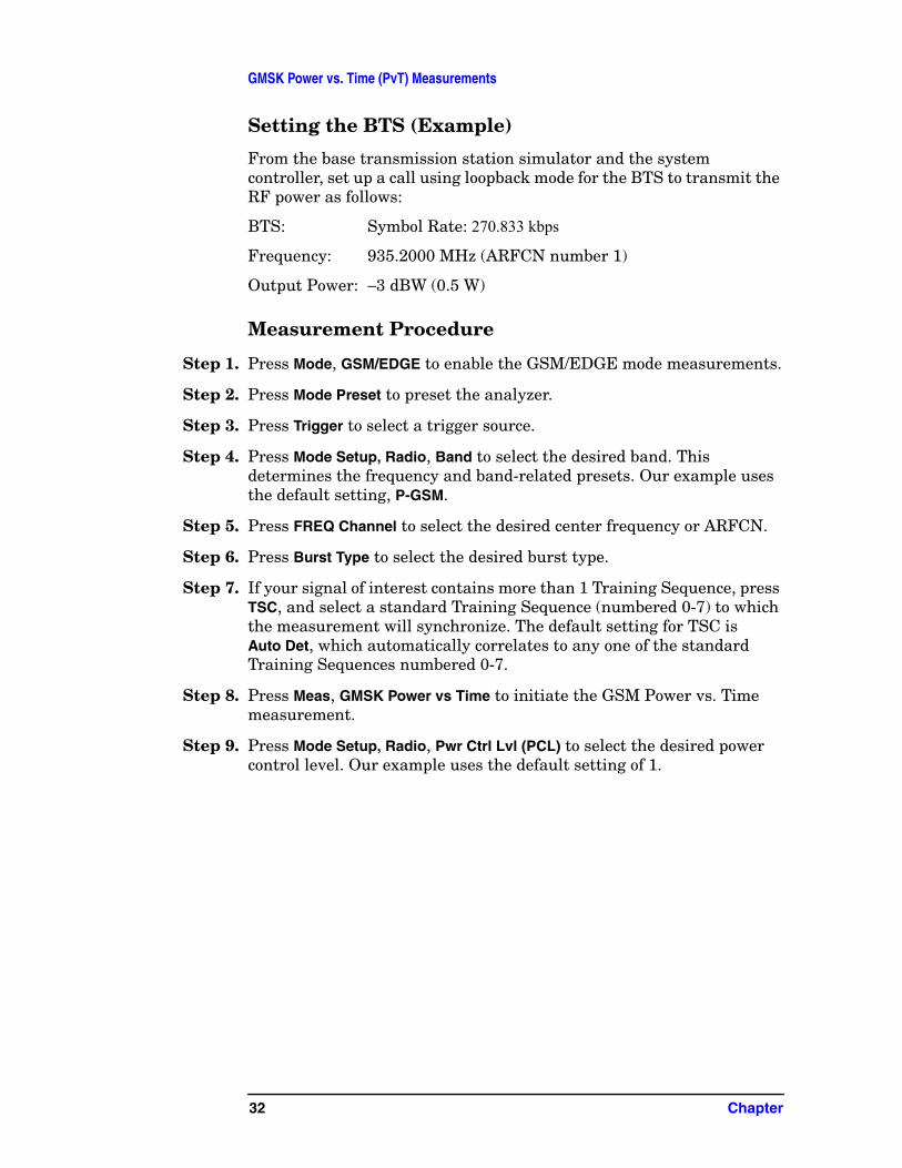
Setting the BTS (Example)
From the base transmission station simulator and the system controller, set up a call using loopback mode for the BTS to transmit the RF power as follows:
Chapter 27
Transmit Power Measurements
BTS: Symbol Rate: 270.833 kbps
Frequency: 935.2000 MHz (ARFCN number 1)
Output Power: −3 dBW (0.5 W)
Measurement Procedure
Step 1. Press Mode, GSM/EDGE to enable the GSM/EDGE mode measurements.
Step 2. Press Mode Preset to preset the analyzer.
Step 3. Press Trigger to select a trigger source.
Step 4. Press FREQ Channel to select the desired center frequency or ARFCN.
Step 5. Press Meas, Transmit Pwr to initiate the Transmit Power measurement.
Figure 3-2 Transmit Power Result - Single Burst, RF Envelope
The Transmit Power measurement result display should look similar Figure 3-2, with a time domain display of the burst waveform plotted in dB, and the power measurement values displayed below.
Both the averaged and instantaneous results for Mean Transmit Power are displayed on the screen of the analyzer. The Averaged Mean Transmit Power Above Threshold is displayed on the left of the display, while the value of the Mean Transmit Power Above Threshold for the current acquisition is displayed on the right of the screen under the heading Current Data Output Pwr. If averaging is turned off, the two values can be the same. When you turn averaging on the Mean Transmit Power Above Threshold is an averaged value.
Step 6. Press Meas Setup to check the keys available to change the measurement parameters from the default condition.
28 Chapter
Transmit Power Measurements
For More Information
For more details about changing measurement parameters, see “Transmit Power (Burst Power) Measurement Concepts” on page 92.
If you have a problem, and get an error message, refer to the Instrument Messages manual.
Troubleshooting Hints
Low output power can lead to poor coverage and intermittent service for phone users. Out of specification power measurements indicate a fault usually in the power amplifier circuitry. They can also provide early indication of a fault with the power supply, for example the battery in the case of mobile stations.
Chapter 29
Transmit Power Measurements
30 Chapter
GMSK Power vs. Time (PvT) Measurements
GMSK Power vs. Time (PvT) MeasurementsThis section explains how to make a GMSK Power versus Time (PvT) measurement on a GSM base station (BTS). Good PvT measurement results verify that the transmitter output power has the correct amplitude, shape, and timing for the GSM format.
NOTE This measurement is designed for GSM. For the EDGE PvT measurement see “EDGE Power vs. Time (PVT) Measurements” on page 55.
Configuring the Measurement System
This example shows a base station (BTS) under test set up to transmit RF power, and being controlled remotely by a system controller. The transmitting signal is connected to the analyzer RF input port. Connect the equipment as shown.
Figure 3-3 GMSK Pwr vs. Time Measurement System
1. Using the appropriate cables, adapters, and circulator, connect the output signal of the BTS to the RF input of the analyzer.
2. Connect the base transmission station simulator or signal generator to the BTS through a circulator to initiate a link constructed with sync and pilot channels, if required.
3. Connect a BNC cable between the 10 MHz OUT port of the signal generator and the EXT REF IN port of the analyzer.
4. Connect the system controller to the BTS through the serial bus cable to control the BTS operation.
Chapter 31
GMSK Power vs. Time (PvT) Measurements
Setting the BTS (Example)
From the base transmission station simulator and the system controller, set up a call using loopback mode for the BTS to transmit the RF power as follows:
BTS: Symbol Rate: 270.833 kbps
Frequency: 935.2000 MHz (ARFCN number 1)
Output Power: −3 dBW (0.5 W)
Measurement Procedure
Step 1. Press Mode, GSM/EDGE to enable the GSM/EDGE mode measurements.
Step 2. Press Mode Preset to preset the analyzer.
Step 3. Press Trigger to select a trigger source.
Step 4. Press Mode Setup, Radio, Band to select the desired band. This determines the frequency and band-related presets. Our example uses the default setting, P-GSM.
Step 5. Press FREQ Channel to select the desired center frequency or ARFCN.
Step 6. Press Burst Type to select the desired burst type.
Step 7. If your signal of interest contains more than 1 Training Sequence, press TSC, and select a standard Training Sequence (numbered 0-7) to which the measurement will synchronize. The default setting for TSC is Auto Det, which automatically correlates to any one of the standard Training Sequences numbered 0-7.
Step 8. Press Meas, GMSK Power vs Time to initiate the GSM Power vs. Time measurement.
Step 9. Press Mode Setup, Radio, Pwr Ctrl Lvl (PCL) to select the desired power control level. Our example uses the default setting of 1.
32 Chapter
GMSK Power vs. Time (PvT) Measurements
Results
The views available under the View/Display menu are Burst, Rise & Fall, and Multi-Slot.
Information shown in the settings panel at the top of the displays include:
• Atten - This value reflects the Internal RF Atten setting.
• Sync - The Burst Sync setting used in the current measurement
• Trig - The Trigger Source setting used in the current measurement
The Mean Transmit Power is displayed at the bottom left of the Burst and Rise & Fall views:
• Mean Transmit Power - This is the RMS average power across the “useful” part of the burst, or the 147 bits centered on the transition from bit 13 to bit 14 (the “T0” time point) of the 26 bit training sequence. An RMS calculation is performed and displayed regardless of the averaging mode selected for the trace data.
If Averaging is set to On, the result displayed is the RMS average power of all bursts measured. If Averaging is set to Off, the result is the RMS average power of the single burst measured. This is a different measurement result from Mean Transmit Power, below.
The Current Data displayed at the bottom of the Burst and Rise & Fall views include:
• Mean Transmit Power - This result appears only if Averaging is set to On. It is the RMS average of power across the “useful” part of the burst, for the current burst only. If a single measurement of “n” averages has been completed, the result indicates the Mean Transmit Power of the last burst. The RMS calculation is performed and displayed regardless of the averaging mode selected for the trace data. This is a different measurement result from Mean Transmit Power, above.
• Max Pt. - Maximum signal power point of the most recently acquired data, in dBm
• Min Pt. - Minimum signal power point of the most recently acquired data, in dBm
• Burst Width - Time duration of burst at −3 dB below the mean power in the useful part of the burst
• 1st Error Pt - (Error Point) The time (displayed in ms or µs) indicates the point on the X Scale where the first failure of a signal was detected. Use a marker to locate this point in order to examine the nature of the failure. The 1st Error Pt. date is displayed only when there is an limit failure.
Chapter 33
GMSK Power vs. Time (PvT) Measurements
Figure 3-4 GMSK Power vs. Time Result - Burst View
Figure 3-5 GMSK Power vs. Time Result - Rise & Fall View
34 Chapter
GMSK Power vs. Time (PvT) Measurements
Figure 3-6 GMSK Power vs. Time Result - Multi-Slot View (5 slots shown)
The table in the lower portion of the multi-slot view shows the output power in dBm for each timeslot, as determined by the integer (1 to 8) entered in the Meas Setup, Meas Time setting. Output power levels are presented for the active slots. A dashed line appears for any slot that is inactive. The timeslot that contains the burst of interest is highlighted in blue.
For more information on making measurements of two consecutive bursts, including the SCPI commands used to make the measurement, refer to the section in the User’s and Programmer’s Reference manual.
For More Information
For more details about changing measurement parameters, see “EDGE Power vs. Time Measurement Concepts” on page 110.
If you have a problem, and get an error message, refer to the Instrument Messages manual.
Troubleshooting Hints
If a transmitter fails the Power vs. Time measurement this usually indicates a problem with the units output amplifier or leveling loop.
Chapter 35
GMSK Power vs. Time (PvT) Measurements
36 Chapter
GMSK Phase and Frequency Error Measurements
GMSK Phase and Frequency Error MeasurementsThis section explains how to make a GMSK Phase and Frequency Error measurement on a GSM base station (BTS). Good measurement results verify modulation quality of the 0.3 GMSK signal for GSM systems. The modulation quality indicates the carrier to noise performance of the system, which is critical for mobiles with low signal levels, at the edge of a cell, or under difficult fading or Doppler conditions.
NOTE This measurement is designed for GSM only.
Configuring the Measurement System
This example shows a base station (BTS) under test set up to transmit RF power, and being controlled remotely by a system controller. The transmitting signal is connected to the analyzer RF input port. Connect the equipment as shown.
Figure 3-7 GMSK Phase and Frequency Measurement System
1. Using the appropriate cables, adapters, and circulator, connect the output signal of the BTS to the RF input of the analyzer.
2. Connect the base transmission station simulator or signal generator to the BTS through a circulator to initiate a link constructed with sync and pilot channels, if required.
3. Connect a BNC cable between the 10 MHz OUT port of the signal generator and the EXT REF IN port of the analyzer.
4. Connect the system controller to the BTS through the serial bus
Chapter 37
GMSK Phase and Frequency Error Measurements
cable to control the BTS operation.
Setting the BTS (Example)
From the base transmission station simulator and the system controller, set up a call using loopback mode for the BTS to transmit the RF power as follows:
BTS: Symbol Rate: 270.833 kbps
Frequency: 935.2000 MHz (ARFCN number 1)
Output Power: −3 dBW (0.5 W)
Measurement Procedure
Step 1. Press Mode, GSM/EDGE to enable the GSM/EDGE mode measurements.
Step 2. Press Mode Preset to preset the analyzer.
Step 3. Press Trigger to select a trigger source.
Step 4. Press FREQ Channel to select the desired center frequency or ARFCN.
Step 5. Press Burst Type to select the desired burst type.
Step 6. If your signal of interest contains more than 1 Training Sequence, press TSC, and select a standard Training Sequence (numbered 0-7) to which the measurement will synchronize. The default setting for TSC is Auto, which automatically correlates to any one of the standard Training Sequences numbered 0-7.
Step 7. Press Meas, GMSK Phase & Freq to initiate the Phase and Frequency Error measurement.
38 Chapter
GMSK Phase and Frequency Error Measurements
Figure 3-8 GMSK Phase and Frequency Error Result - Quad View (Default)
Step 8. Press Zoom and then Next Window to expand each of the quadrants for closer inspection.
Step 9. Press View/Display, I/Q Measured Polar Graph to view the Polar plot of vector data and the Phase and Frequency Error summaries.
Figure 3-9 GMSK Phase and Frequency Error Result - Polar View
Chapter 39
GMSK Phase and Frequency Error Measurements
Step 10. Press View/Display, Data Bits to display the Phase Error vs. Frequency information.
NOTE The demodulated bits in this display are Symbol State bits, and do not represent encoded message data.
Figure 3-10 GMSK Phase and Frequency Error Result - Data Bits
For More Information
For more details about changing measurement parameters, see “GMSK Phase and Frequency Error Measurement Concepts” on page 101.
If you have a problem, and get an error message, refer to the Instrument Messages manual.
Troubleshooting Hints
Poor phase error indicates a problem with the I/Q baseband generator, filters, or modulator in the transmitter circuitry. The output amplifier in the transmitter can also create distortion that causes unacceptably high phase error. In a real system. poor phase error reduces the ability of a receiver to correctly demodulate, especially in marginal signal conditions. This ultimately affects range.
Occasionally, a Phase and Frequency Error measurement may fail the prescribed limits at only one point in the burst, for example at the beginning. This could indicate a problem with the transmitter power ramp or some undesirable interaction between the modulator and power amplifier.
40 Chapter
GMSK Output RF Spectrum (ORFS) Measurements
GMSK Output RF Spectrum (ORFS) MeasurementsThis section explains how to make a GSM Output RF Spectrum measurement on a base station. This test verifies that the modulation, wideband noise, and power level switching spectra are within limits and do not produce significant interference in the adjacent base transceiver station (BTS) channels.
NOTE This measurement is designed for GSM. For the EDGE Output RF Spectrum measurement see “EDGE Output RF Spectrum (ORFS) Measurements” on page 67.
Configuring the Measurement System
This example shows a base station (BTS) under test set up to transmit RF power, and being controlled remotely by a system controller. The transmitting signal is connected to the analyzer RF input port. Connect the equipment as shown.
Figure 3-11 GMSK ORFS Measurement System
1. Using the appropriate cables, adapters, and circulator, connect the output signal of the BTS to the RF input of the analyzer.
2. Connect the base transmission station simulator or signal generator to the BTS through a circulator to initiate a link constructed with sync and pilot channels, if required.
3. Connect a BNC cable between the 10 MHz OUT port of the signal generator and the EXT REF IN port of the analyzer.
Chapter 41
GMSK Output RF Spectrum (ORFS) Measurements
4. Connect the system controller to the BTS through the serial bus cable to control the BTS operation.
NOTE If the signal being measured has more than one active slot in a frame, the default RF Burst trigger must be changed, and an external event trigger must be provided to synchronize the frame. Otherwise the measurement may trigger randomly on any burst in an active slot. This is true for all ORFS time domain measurements.
Setting the BTS (Example)
From the base transmission station simulator and the system controller, set up a call using loopback mode for the BTS to transmit the RF power as follows:
BTS: Symbol Rate: 270.833 kbps
Frequency: 935.2000 MHz (ARFCN number 1)
Output Power: −3 dBW (0.5 W)
Measurement Procedure
Step 1. Press Mode, GSM/EDGE to enable the GSM/EDGE mode measurements.
Step 2. Press Mode Preset to preset the analyzer.
Step 3. Press Trigger to select a trigger source.
Step 4. Press FREQ Channel to select the desired center frequency or ARFCN.
Step 5. Press Burst Type to select the desired burst type.
Step 6. If your signal of interest contains more than 1 Training Sequence, press TSC, and select a standard Training Sequence (numbered 0-9) to which the measurement will synchronize. The default setting for TSC is Auto, which automatically correlates to any one of the standard Training Sequences numbered 0-9. Training Sequence synchronization is applicable only when Periodic Timer Trigger and Periodic Time Sync Source are off.
Step 7. Press Meas, GMSK Output RF Spectrum to initiate the GMSK Output RF Spectrum (ORFS) measurements.
42 Chapter
GMSK Output RF Spectrum (ORFS) Measurements
Step 8. Press Meas Setup and select the Meas Type and Meas Method for your measurement:
• Meas Type - Accesses a menu to choose the measurement that is optimized for the type of spectral distortion being investigated.
Mod & Switch - Performs both Modulation and Switching measurements, which measures the spectrum due to the 0.3 GMSK modulation and noise, and Switching (transient) measurements.
Modulation - Measures the spectrum optimized for distortion due to the 0.3 GMSK modulation and noise.
Switching - Measures the spectrum optimized for distortion due to switching transients (burst ramping).
Full Frame Modulation (FAST)- Improves measurement speed by acquiring a full frame of data and reduces actual average number. This feature can only be used when all slots in the transmitted frame are active. Use of an external trigger can enhance measurement speed when this feature is used. When Full Frame Modulation (FAST) is selected, the current measurement defaults to the multi-offset measurement method. Therefore, the single offset key and swept key in Meas Method menu are grayed out and these two features are not available.
• Meas Method - Accesses a menu to choose the measurement mode.
Multi-Offset - Automatically makes measurements at all offset frequencies in the selected list (Standard, Short, or Custom). Press Multi-Offset Freq List to select a list of offsets to measure.
Multi-Offset measurements may be made with either Modulation or Switching measurement types.
Offset measurement results are displayed as tabular data.
Single Offset (Examine) - Makes a measurement at a single offset frequency as set by the Single Offset Freq softkey. This allows detailed examination of the time-domain waveform at the specified offset frequency.
Single Offset (Examine) measurements may be made with either Modulation or Switching measurement types.
Single offset measurement results are displayed in a time domain plot, with the measurement offset shown as a gate by white vertical lines. See Figure 3-13 on page 45.
Swept - Makes a measurement using time-gated spectrum analysis to sweep the analyzer with the gate turned on for the desired portion of the burst when Meas Type is set to Modulation. When Meas Type is set to Switching, turns off the gate and
Chapter 43
GMSK Output RF Spectrum (ORFS) Measurements
sweeps with peak detector and appropriate sweep time. The limits mask is applied to the spectrum plot, and the Worst Frequency parameters are displayed. This selection is only available if Meas Type is set to Modulation or Switching. See Figure 3-16 on page 48.
Step 9. Press Restart to re-initiate a GMSK ORFS measurement if you change the Meas Type or Meas Method. You can also set Meas Control to Measure Cont for continuous measurements.
GMSK ORFS Measurement Results
• Modulation Power - When Meas Method is set to Multi-Offset, and Meas Type is set to Modulation, Mod and Switch, or Full Frame Modulation, measurement results may be viewed as absolute powers in tabular form. The data displays offsets from any of the Multi-Offset Freq List settings: Standard, Short, and Custom. The Modulation Power view is the default view for ORFS measurements.
Figure 3-12 GMSK ORFS - Example (Short List) Modulation Power View
44 Chapter
GMSK Output RF Spectrum (ORFS) Measurements
• Single Offset (Examine) - Makes a measurement at a single offset frequency as set by the Offset Freq softkey.
Single offset measurement results are displayed as a power waveform in a time domain plot, with the measurement offset shown as a gate by white vertical lines. The red vertical lines represent the additional effective measurement window when Fast Avg is ON (default setting).
You can select the Single Offset (Examine) view by pressing Meas Setup, Meas Method, and then Single Offset (Examine).
NOTE The signal being displayed below is the useful part of slot 0, which in this example, is the only active slot in the frame. If any other slots are active, the default RF Burst trigger must be changed, and an external event trigger must be provided to synchronize the frame. Otherwise the measurement may trigger randomly on any burst in an active slot. This is true for all ORFS time domain measurements.
Figure 3-13 GMSK ORFS Result - Modulation Single Offset (Examine) View
Chapter 45
GMSK Output RF Spectrum (ORFS) Measurements
• Switching Single Offset measurement results are displayed in a time domain plot, but the waveform of the entire frame is displayed. In this example, slots 0, 1, and 4 are active. Use the external trigger to maintain frame synchronization. Fast Avg is not available for this measurement.
Figure 3-14 GMSK ORFS Result - Switching Single Offset (Examine) View
46 Chapter
GMSK Output RF Spectrum (ORFS) Measurements
• Combination Modulation and Switching (Mod & Switch) Single Offset measurement results are displayed in a time domain plot, but the waveform of the entire frame is displayed. The blue trace is the Switching data and the yellow trace is the Modulation data, with the measurement gates shown.
In this example, slots 1 and 4 are active. Use the external trigger to maintain frame synchronization. Fast Avg is not available for this measurement.
Figure 3-15 GMSK ORFS Result - Mod & Switch Single Offset (Examine) View
Chapter 47
GMSK Output RF Spectrum (ORFS) Measurements
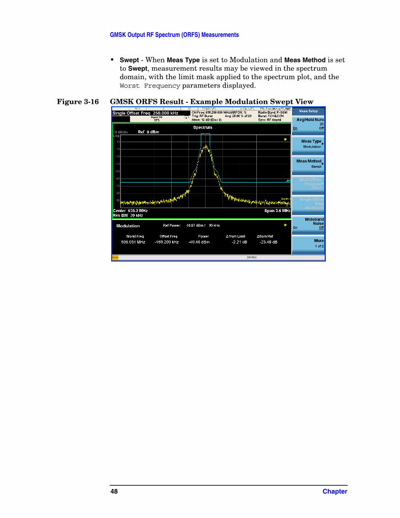
• Swept - When Meas Type is set to Modulation and Meas Method is set to Swept, measurement results may be viewed in the spectrum domain, with the limit mask applied to the spectrum plot, and the Worst Frequency parameters displayed.
Figure 3-16 GMSK ORFS Result - Example Modulation Swept View
48 Chapter
GMSK Output RF Spectrum (ORFS) Measurements
• Swept - When Meas Type is set to Switching and Meas Method is set to Swept, measurement results may be viewed in the spectrum domain, with the limit mask applied to the spectrum plot, and the Worst Frequency parameters displayed.
Figure 3-17 GMSK ORFS Result - Example Switching Swept View
Chapter 49
GMSK Output RF Spectrum (ORFS) Measurements
• Full Frame Mode (FAST) - When Meas Method is set to Multi-Offset, and Meas Type is set to Full Frame Mode (FAST), measurement results may be viewed as relative and absolute powers in tabular form. The data displays offsets from any of the Multi-Offset Freq List settings: Standard, Short, and Custom.
To measure Full Frame Mode (FAST), all slots in the frame must be active. In the example below, slots 6 and 7 were inactive and Multi-Offset Freq List is set to Standard.
Figure 3-18 GMSK ORFS Result - Full Frame Modulation (FAST) View
For More Information
For more details about changing measurement parameters, see “GMSK Output RF Spectrum Measurement Concepts” on page 104.
If you have a problem, and get an error message, refer to the Instrument Messages manual.
50 Chapter
GMSK Transmitter Band Spurious Signal (Tx Band Spur) Measurements
GMSK Transmitter Band Spurious Signal (Tx Band Spur) MeasurementsThis section explains how to make a GMSK Tx Band Spur measurement on a GSM base station (BTS). Good measurement results verify that the transmitter does not transmit undesirable energy into the transmit band. If undesirable energy is present, it may cause interference for other users of the GSM system.
NOTE This measurement is designed for GSM BTS testing only. For the EDGE Tx Band Spur measurement see “EDGE Transmitter Band Spur Measurements” on page 77.
Configuring the Measurement System
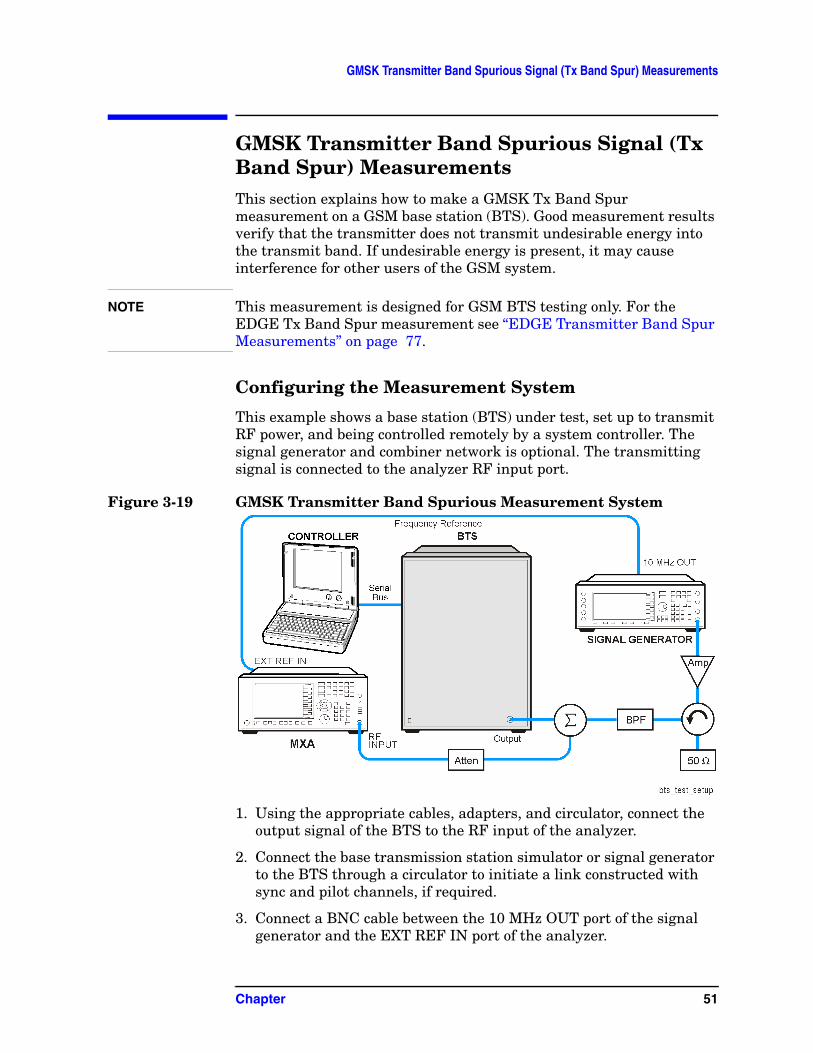
This example shows a base station (BTS) under test, set up to transmit RF power, and being controlled remotely by a system controller. The signal generator and combiner network is optional. The transmitting signal is connected to the analyzer RF input port.
Figure 3-19 GMSK Transmitter Band Spurious Measurement System
1. Using the appropriate cables, adapters, and circulator, connect the output signal of the BTS to the RF input of the analyzer.
2. Connect the base transmission station simulator or signal generator to the BTS through a circulator to initiate a link constructed with sync and pilot channels, if required.
3. Connect a BNC cable between the 10 MHz OUT port of the signal generator and the EXT REF IN port of the analyzer.
Chapter 51
GMSK Transmitter Band Spurious Signal (Tx Band Spur) Measurements
4. Connect the system controller to the BTS through the serial bus cable to control the BTS operation.
Setting the BTS (Example)
From the base transmission station simulator and the system controller, set up a call using loopback mode for the BTS to transmit the RF power as follows:
BTS: Symbol Rate: 270.833 kbps
Frequency: 935.2000 MHz (ARFCN number 1)
Output Power: −3 dBW (0.5 W)
Measurement Procedure
Step 1. Press Mode, GSM/EDGE to enable the GSM/EDGE mode measurements.
Step 2. Press Mode Preset to preset the analyzer.
Step 3. Press FREQ Channel to select the desired center frequency or ARFCN.
Step 4. Press Meas, GMSK Tx Band Spur to initiate the Transmitter Band Spurious products measurement.
Results
Figure 3-20 GMSK Tx Band Spur Result - Upper Segment
52 Chapter
GMSK Transmitter Band Spurious Signal (Tx Band Spur) Measurements
For More Information
For more details about changing measurement parameters, see “GMSK Tx Band Spur Measurement Concepts” on page 108.
If you have a problem, and get an error message, refer to the Instrument Messages manual.
Troubleshooting Hints
Almost any fault in the transmitter circuits can manifest itself as spurious of one kind or another. Make sure the transmit band is correctly selected and the frequency is either the Bottom, Middle, or Top channel. The “Carrier freq not allowed with BMT (Bottom/Middle/Top only)” message usually indicates the transmit band and/or carrier frequency is not correct.
Chapter 53
GMSK Transmitter Band Spurious Signal (Tx Band Spur) Measurements
54 Chapter
EDGE Power vs. Time (PVT) Measurements
EDGE Power vs. Time (PVT) MeasurementsThis section explains how to make an EDGE Power versus Time (PvT) measurement on an EDGE base station. Good PvT measurement results verify that the transmitter output power has the correct amplitude, shape, and timing for the EDGE format.
NOTE This measurement is designed for EDGE. For the GSM PvT measurement see “GMSK Power vs. Time (PvT) Measurements” on page 31.
Configuring the Measurement System
This example shows a base station (BTS) under test set up to transmit RF power, and being controlled remotely by a system controller. The transmitting signal is connected to the analyzer RF input port. Connect the equipment as shown.
Figure 3-21 EDGE Pwr vs. Time Measurement System
1. Using the appropriate cables, adapters, and circulator, connect the output signal of the BTS to the RF input of the analyzer.
2. Connect the base transmission station simulator or signal generator to the BTS through a circulator to initiate a link constructed with sync and pilot channels, if required.
3. Connect a BNC cable between the 10 MHz OUT port of the signal generator and the EXT REF IN port of the analyzer.
4. Connect the system controller to the BTS through the serial bus cable to control the BTS operation.
Chapter 55
EDGE Power vs. Time (PVT) Measurements
Setting the BTS (Example)
From the base transmission station simulator and the system controller, set up a call using loopback mode for the BTS to transmit the RF power as follows:
BTS: Symbol Rate: 270.833 kbps
Frequency: 935.2000 MHz (ARFCN number 1)
Output Power: −3 dBW (0.5 W)
Measurement Procedure
Step 1. Press Mode, GSM/EDGE to enable the GSM/EDGE mode measurements.
Step 2. Press Mode Preset to preset the analyzer.
Step 3. Press Trigger to select a trigger source.
Step 4. Press Radio, Band to select the desired band. This will determine the frequency and band-related presets. Our example will use the default setting, P-GSM.
Step 5. Press FREQ Channel to select the desired center frequency or ARFCN.
Step 6. Press Burst Type to select the desired burst type.
Step 7. If your signal of interest contains more than 1 Training Sequence, press TSC, and select a standard Training Sequence (numbered 0-7) to which the measurement will synchronize. The default setting for TSC is Auto Det, which will automatically correlate to any one of the standard Training Sequences numbered 0-7.
Step 8. Press Meas, EDGE Power vs Time to initiate the EDGE Power vs. Time measurement.
Step 9. Press Mode Setup, Radio, Pwr Cntl Level (PCL) to select the desired power control level. Our example uses the default setting of 1.
56 Chapter
EDGE Power vs. Time (PVT) Measurements
Results
The views available under the View/Display menu are Burst, Rise & Fall, and Multi-Slot.
Information shown in the settings panel at the top of the displays include:
• Atten - This value reflects the Internal RF Atten setting.
• Sync - The Burst Sync setting used in the current measurement
• Trig - The Trigger Source setting used in the current measurement
The Mean Transmit Power is displayed at the bottom left of the Burst and Rise & Fall views:
• Mean Transmit Power - This is the RMS average power across the “useful” part of the burst, or the 147 bits centered on the transition from bit 13 to bit 14 (the “T0” time point) of the 26 bit training sequence. An RMS calculation is performed and displayed regardless of the averaging mode selected for the trace data.
If Averaging is set to On, the result displayed is the RMS average power of all bursts measured. If Averaging is set to Off, the result is the RMS average power of the single burst measured. This is a different measurement result from Mean Transmit Power, below.
The Current Data displayed at the bottom of the Burst and Rise & Fall views include:
• Mean Transmit Power - This result appears only if Averaging = ON. It is the RMS average of power across the “useful” part of the burst, for the current burst only. If a single measurement of “n” averages has been completed, the result indicates the Mean Transmit Power of the last burst. The RMS calculation is performed and displayed regardless of the averaging mode selected for the trace data. This is a different measurement result from Mean Transmit Power, above.
• Max Pt. - Maximum signal power point of the most recently acquired data, in dBm
• Min Pt. - Minimum signal power point of the most recently acquired data, in dBm
• Burst Width - Time duration of burst at −3 dB below the mean power in the useful part of the burst
• Mask Ref Pwr Midamble - The Mask Reference Power is the average power in dBm of the middle 16 symbols in the midamble. The times displayed are the corresponding start and stop times of the middle 16 symbols.
• 1st Error Pt - (Error Point) The time (displayed in ms or µs)
Chapter 57
EDGE Power vs. Time (PVT) Measurements
indicates the point on the X Scale where the first failure of a signal was detected. Use a marker to locate this point in order to examine the nature of the failure. The 1st Error Pt. date is displayed only when there is an limit failure.
Figure 3-22 EDGE Power vs. Time Result - Burst View
Figure 3-23 EDGE Power vs. Time Result - Rise & Fall View
58 Chapter
EDGE Power vs. Time (PVT) Measurements
Figure 3-24 EDGE Result - Multi-Slot View (3 slots shown)
The table in the lower portion of the multi-slot view shows the output power in dBm for each timeslot, as determined by the integer (1 to 8) entered in the Meas Setup, Meas Time setting. Output power levels are presented for the active slots; a dashed line will appear for any slot that is inactive. The timeslot that contains the burst of interest is highlighted in blue.
Use the Meas Time key located in the Meas Setup menu to select up to eight slots. Use the Time Slot and TSC keys in the FREQ/Channel menu to select the slot you wish to activate. Setting Time Slot to ON and selecting a specific slot results in activating a measurement of that slot only (Time Slot On can be used to isolate a failure to a specific slot). When Time Slot is set to OFF, all active slots are tested against the mask.
Using a signal generator you can synchronize the multi-slot view so the frame (or portion of the frame) you are viewing starts with the slot you have selected. See “EDGE Power vs. Time Measurement Concepts” on page 110.
You can switch from the multi-slot view directly to the burst or rise and fall views of the slot that is currently active. The Scale/Div key under the Span/X Scale menu can be used to enlarge your view of this signal.
For More Information
For more details about changing measurement parameters, see “EDGE Power vs. Time Measurement Concepts” on page 110.
If you have a problem, and get an error message, refer to the Instrument Messages manual.
Chapter 59
EDGE Power vs. Time (PVT) Measurements
Troubleshooting Hints
If a transmitter fails the Power vs. Time measurement this usually indicates a problem with the units output amplifier or leveling loop.
60 Chapter
EDGE Error Vector Magnitude (EVM) Measurements
EDGE Error Vector Magnitude (EVM) MeasurementsThis section explains how to make an EDGE Error Vector Magnitude (EVM) measurement on an EDGE base station. EVM provides a measure of modulation accuracy. The EDGE 8 PSK modulation pattern uses a rotation of 3π/8 radians to avoid zero crossing, thus providing a margin of linearity relief for amplifier performance.
NOTE This is an EDGE only measurement.
Configuring the Measurement System
This example shows a base station (BTS) under test set up to transmit RF power, and being controlled remotely by a system controller. The transmitting signal is connected to the analyzer RF input port. Connect the equipment as shown.
Figure 3-25 EDGE EVM Measurement System
1. Using the appropriate cables, adapters, and circulator, connect the output signal of the BTS to the RF input of the analyzer.
2. Connect the base transmission station simulator or signal generator to the BTS through a circulator to initiate a link constructed with sync and pilot channels, if required.
3. Connect a BNC cable between the 10 MHz OUT port of the signal generator and the EXT REF IN port of the analyzer.
4. Connect the system controller to the BTS through the serial bus cable to control the BTS operation.
Chapter 61
EDGE Error Vector Magnitude (EVM) Measurements
Setting the BTS (Example)
From the base transmission station simulator and the system controller, set up a call using loopback mode for the BTS to transmit the RF power as follows:
BTS: Symbol Rate: 270.833 kbps
Frequency: 935.2000 MHz (ARFCN number 1)
Output Power: −3 dBW (0.5 W)
Measurement Procedure
Step 1. Press Mode, GSM/EDGE to enable the GSM/EDGE mode measurements.
Step 2. Press Mode Preset to preset the analyzer.
Step 3. Press Trigger to select a trigger source.
Step 4. Press FREQ Channel to select the desired center frequency or ARFCN.
Step 5. Press Burst Type to select the desired burst type.
Step 6. If your signal of interest contains more than 1 Training Sequence, press TSC, and select a standard Training Sequence (numbered 0-9) to which the measurement will synchronize. The default setting for TSC is Auto Det, which automatically correlates to any one of the standard Training Sequences numbered 0-9.
Step 7. Press Meas, EDGE EVM to initiate the EDGE Error Vector Magnitude measurement.
Figure 3-26 on page 63 shows an example of measurement result with the graphic and text windows. The measured summary data is shown in the left window and the dynamic vector trajectory of the I/Q demodulated signal is shown as a polar vector display in the right window.
The analyzer searches the training sequence on the amplitude path and phase path and try to sync. Polar modulation analysis measures the time delay adjustment between the Amplitude path and Phase path for Polar modulation. When Polar Modulation is selected, the timing offset of amplitude path to phase path is always calculated.
The displayed time delay values are called AMPM Offset and T0 Offset. They are shown in the I/Q Measured Polar Graph view, I/Q Error view, and Data bits view. You can select time (seconds) or symbols as the display unit using Time Offset Unit in the Display key menu.
The Polar Mod Align On/Off key located in the Meas Setup menu. The Polar Mod Align setting determines whether the timing offsets are used
62 Chapter
EDGE Error Vector Magnitude (EVM) Measurements
(when set to On) for compensation in the EVM calculation.
Figure 3-26 EDGE EVM Result - Polar Graph View
Chapter 63
EDGE Error Vector Magnitude (EVM) Measurements
Step 9. Press View/Display, I/Q Error to display a four-pane view of the Magnitude Error, Phase Error, and EVM graphs, along with a summary of the measurement data. You can select any of the graph windows for individual display or adjustment by pressing Next WIndow and moving the green selection box to the desired window. Press Zoom to expand the window to full screen, or to go back to the Quad-View.
In the example below, a sine modulation is apparent in the EVM and Phase Error data. This could due to an FM impairment that is not discernible in the other EVM views.
Figure 3-27 EDGE EVM Result - I/Q Error
64 Chapter
EDGE Error Vector Magnitude (EVM) Measurements
Step 10. Press View/Display, Data Bits to display a summary of measurement data along with the symbol state bits. The training sequence is highlighted in blue, and remains constant with repeated measurement updates.
Figure 3-28 EDGE EVM Result - Data Bits View
NOTE The data bits in this display are Symbol State bits, and do not represent encoded message data.
For More Information
For more details about changing measurement parameters, see “EDGE EVM Measurement Concepts” on page 117.
If you have a problem, and get an error message, refer to the Instrument Messages manual.
Troubleshooting Hints
Use the spectrum (frequency domain) measurement to verify that the signal is present and approximately centered on the display.
The data used for testing can have a detrimental effect on the EVM results, causing erratic or falsely high EVM, especially in the case of sending all 0 bits with the Trigger Source set to RF Burst. In that unique situation, better results may be obtained using Free Run or Video triggers.
Poor EVM indicates a problem at the I/Q baseband generator, filters, and/or modulator in the transmitter circuitry. The output amplifier in the transmitter can also create distortion that causes unacceptably
Chapter 65
EDGE Error Vector Magnitude (EVM) Measurements
high EVM. In a real system, poor EVM reduces the ability of a receiver to correctly demodulate the signal, especially in marginal signal conditions. Poor EVM may also indicate that a measurement restart was not performed after the signal level was changed. Press Restart after a change in the input signal to ensure that an auto-attenuation adjustment is performed.
The I/Q Error Quad View display may be used to determine where modulation or demodulation errors are introduced into the complex modulated path.
66 Chapter
EDGE Output RF Spectrum (ORFS) Measurements
EDGE Output RF Spectrum (ORFS) MeasurementsThis section explains how to make an EDGE Output RF Spectrum measurement on an EDGE base station. This test verifies that the modulation, wideband noise, and power level switching spectra are within limits and do not produce significant interference in the adjacent base transceiver station (BTS) channels.
NOTE This measurement is designed for EDGE. For the GSM Output RF Spectrum measurement see “GMSK Output RF Spectrum (ORFS) Measurements” on page 41.
Configuring the Measurement System
This example shows a base transceiver station (BTS) under test set up to transmit RF power, and being controlled remotely by a system controller. The transmitting signal is connected to the analyzer RF input port. Connect the equipment as shown.
Figure 3-29 EDGE ORFS Measurement System
1. Using the appropriate cables, adapters, and circulator, connect the output signal of the BTS to the RF input of the analyzer.
2. Connect the base transmission station simulator or signal generator to the BTS through a circulator to initiate a link constructed with sync and pilot channels, if required.
3. Connect a BNC cable between the 10 MHz OUT port of the signal generator and the EXT REF IN port of the analyzer.
Chapter 67
EDGE Output RF Spectrum (ORFS) Measurements
4. Connect the system controller to the BTS through the serial bus cable to control the BTS operation.
NOTE If the signal being measured has more than one active slot in a frame, the default RF Burst trigger must be changed, and an external event trigger must be provided to synchronize the frame. Otherwise the measurement may trigger randomly on any burst in an active slot. This is true for all ORFS time domain measurements.
Setting the BTS (Example)
From the base transmission station simulator and the system controller, set up a call using loopback mode for the BTS to transmit the RF power as follows:
BTS: Symbol Rate: 270.833 kbps
Frequency: 935.2000 MHz (ARFCN number 1)
Output Power: −3 dBW (0.5 W)
Measurement Procedure
Step 1. Press Mode, GSM/EDGE to enable the GSM/EDGE mode measurements.
Step 2. Press Mode Preset to preset the analyzer.
Step 3. Press Trigger to select a trigger source.
Step 4. Press Mode Setup, Demod, Burst Align to toggle the burst alignment to 1/2 Bit Offset.
Step 5. Press FREQ Channel to select the desired center frequency or ARFCN.
Step 6. Press FREQ Channel, Burst Type to select the desired burst type.
Step 7. If your signal of interest contains more than 1 Training Sequence, press TSC, and select a standard Training Sequence (numbered 0-9) to which the measurement will synchronize. The default setting for TSC is Auto, which automatically correlates to any one of the standard Training Sequences numbered 0-9. Training Sequence synchronization is applicable only when Periodic Timer Trigger and Periodic Time Sync Source are off.
Step 8. Press Meas, EDGE Output RF Spectrum to initiate the EDGE Output RF Spectrum (ORFS) measurements.
68 Chapter
EDGE Output RF Spectrum (ORFS) Measurements
Step 9. Press Meas Setup and select the Meas Type and Meas Method for your measurement:
• Meas Type - Accesses a menu to choose the measurement that is optimized for the type of spectral distortion being investigated.
Mod & Switch - Performs both Modulation and Switching measurements, which measures the spectrum due to modulation and noise, and also measures Switching (transient) spectrum measurements.
Modulation - Measures the spectrum optimized for distortion due to modulation and noise.
Switching - Measures the spectrum optimized for distortion due to switching transients (burst ramping).
Full Frame Modulation (FAST)- Improves measurement speed by acquiring a full frame of data and reduces actual average number. This feature can only be used when all slots in the transmitted frame are active. Use of an external trigger can enhance measurement speed when this feature is used. When Full Frame Modulation (FAST) is selected the current measurement defaults to the multi-offset measurement method. Therefore, the single offset key and swept key in Meas Method menu are grayed out and these two features are not available.
• Meas Method
Multi-Offset - Automatically makes measurements at all offset frequencies in the selected list (Standard, Short, or Custom). Press Multi-Offset Freq List to select a list of offsets to measure.
Multi-Offset measurements may be made with either Modulation or Switching measurement types.
Offset measurement results are displayed as tabular data.
Single Offset (Examine) - makes a measurement at a single offset frequency as set by the Single Offset Freq softkey.
Single Offset (Examine) measurements may be made with either Modulation or Switching measurement types.
Single offset measurement results are displayed in a time domain plot, with the measurement offset shown as a gate by white vertical lines. See Figure 3-31 on page 71.
Swept - Makes a measurement using time-gated spectrum analysis to sweep the analyzer with the gate turned on for the desired portion of the burst when Meas Type is set to Modulation. When Meas Type is set to Switching, turn off the gate and sweep with peak detector, appropriate sweep time. The limits mask is applied to the spectrum plot, and the Worst Frequency
Chapter 69
EDGE Output RF Spectrum (ORFS) Measurements
parameters are displayed. This selection is only available if Meas Type is set to Modulation. See Figure 3-34 on page 74.
- Accesses a menu to choose the measurement mode.
Step 10. You can also set Meas Control to Measure Cont for continuous measurements.
EDGE ORFS Measurement Results
• Modulation Power - When Meas Method is set to Multi-Offset, and Meas Type is set to Modulation, Mod and Switch, or Full Frame Modulation, measurement results may be viewed as absolute powers in tabular form. The data displays offsets from any of the Multi-Offset Freq List settings: Standard, Short, and Custom. The Modulation Power view is the default view for ORFS measurements.
Figure 3-30 EDGE ORFS - Example (Short List) Modulation Power View
70 Chapter
EDGE Output RF Spectrum (ORFS) Measurements
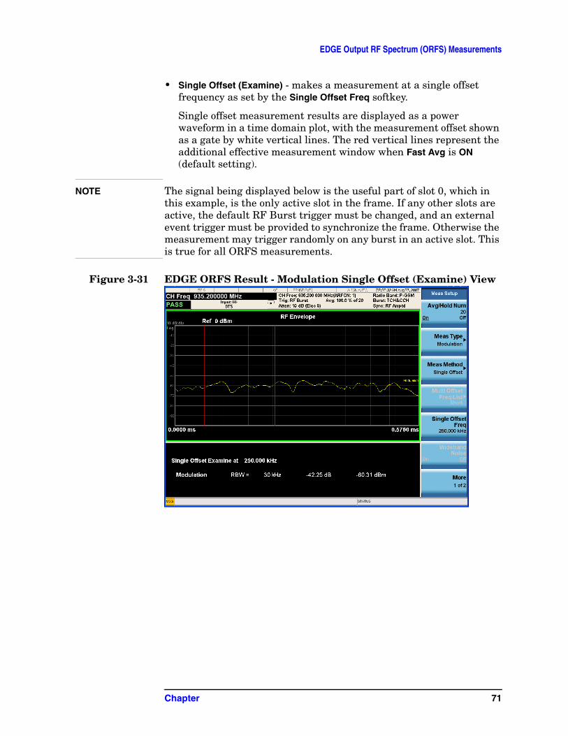
• Single Offset (Examine) - makes a measurement at a single offset frequency as set by the Single Offset Freq softkey.
Single offset measurement results are displayed as a power waveform in a time domain plot, with the measurement offset shown as a gate by white vertical lines. The red vertical lines represent the additional effective measurement window when Fast Avg is ON (default setting).
NOTE The signal being displayed below is the useful part of slot 0, which in this example, is the only active slot in the frame. If any other slots are active, the default RF Burst trigger must be changed, and an external event trigger must be provided to synchronize the frame. Otherwise the measurement may trigger randomly on any burst in an active slot. This is true for all ORFS measurements.
Figure 3-31 EDGE ORFS Result - Modulation Single Offset (Examine) View
Chapter 71
EDGE Output RF Spectrum (ORFS) Measurements
• Switching Single Offset measurement results are displayed in a time domain plot, but the waveform of the entire frame is displayed. In this example, slots 0, 1, and 4 are active. Use the external trigger to maintain frame synchronization. Fast Avg is not available for this measurement.
Figure 3-32 EDGE ORFS Result - Switching Single Offset (Examine) View
72 Chapter
EDGE Output RF Spectrum (ORFS) Measurements
• Combination Modulation and Switching (Mod & Switch) Single Offset measurement results are displayed in a time domain plot, but the waveform of the entire frame is displayed. The blue trace is the Switching data and the yellow trace is the Modulation data, with the measurement gates shown.
In this example, slots 0, 1, and 4 are active. Use the external trigger to maintain frame synchronization. Fast Avg is not available for this measurement.
Figure 3-33 EDGE ORFS Result - Mod & Switch Single Offset (Examine) View
Chapter 73
EDGE Output RF Spectrum (ORFS) Measurements
• Swept - When Meas Type is set to Modulation and Meas Method is set to Swept, measurement results may be viewed in the spectrum domain, with the limit mask applied to the spectrum plot, and the Worst Frequency parameters displayed.
Figure 3-34 EDGE ORFS Result - Example Modulation Swept View
74 Chapter
EDGE Output RF Spectrum (ORFS) Measurements
• Swept - When Meas Type is set to Switching and Meas Method is set to Swept, measurement results may be viewed in the spectrum domain, with the limit mask applied to the spectrum plot, and the Worst Frequency parameters displayed.
Figure 3-35 EDGE ORFS Result - Example Modulation Swept View
Chapter 75
EDGE Output RF Spectrum (ORFS) Measurements
• Full Frame Mode (FAST) - When Meas Method is set to Multi-Offset, and Meas Type is set to Full Frame Mode (FAST), measurement results may be viewed as relative and absolute powers in tabular form. The data displays offsets from any of the Multi-Offset Freq List settings: Standard, Short, and Custom.
To measure Full Frame Mode (FAST), all slots in the frame must be active. In the example below, slots 6 and 7 were inactive and Multi-Offset Freq List is set to Standard.
Figure 3-36 EDGE ORFS Result - Full Frame Modulation (FAST) View
For More Information
For more details about changing measurement parameters, see “EDGE Output RF Spectrum Measurement Concepts” on page 121.
If you have a problem, and get an error message, refer to the Instrument Messages manual.
76 Chapter
EDGE Transmitter Band Spur Measurements
EDGE Transmitter Band Spur MeasurementsThis section explains how to make an EDGE Tx Band Spur measurement on an EDGE base station (BTS). Good measurement results verify that the transmitter does not transmit undesirable energy into the transmit band. This energy may cause interference for other users of the EDGE system.
NOTE This measurement is designed for EDGE BTS testing only. For the GSM Tx Band Spur measurement see “GMSK Transmitter Band Spurious Signal (Tx Band Spur) Measurements” on page 51.
Configuring the Measurement System
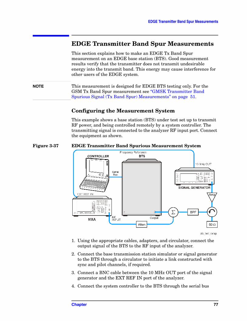
This example shows a base station (BTS) under test set up to transmit RF power, and being controlled remotely by a system controller. The transmitting signal is connected to the analyzer RF input port. Connect the equipment as shown.
Figure 3-37 EDGE Transmitter Band Spurious Measurement System
1. Using the appropriate cables, adapters, and circulator, connect the output signal of the BTS to the RF input of the analyzer.
2. Connect the base transmission station simulator or signal generator to the BTS through a circulator to initiate a link constructed with sync and pilot channels, if required.
3. Connect a BNC cable between the 10 MHz OUT port of the signal generator and the EXT REF IN port of the analyzer.
4. Connect the system controller to the BTS through the serial bus
Chapter 77
EDGE Transmitter Band Spur Measurements
cable to control the BTS operation.
Setting the BTS (Example)
From the base transmission station simulator and the system controller, set up a call using loopback mode for the BTS to transmit the RF power as follows:
BTS: Symbol Rate: 270.833 kbps
Frequency: 935.2000 MHz (ARFCN number 1)
Output Power: −3 dBW (0.5 W)
Measurement Procedure
Step 1. Press Mode, GSM/EDGE to enable the GSM/EDGE mode measurements.
Step 2. Press Mode Preset to preset the analyzer.
Step 3. Press FREQ Channel to select the desired center frequency or ARFCN.
Step 4. Press Meas, Tx Band Spur to initiate the EDGE Transmitter Band Spurious products measurement.
Results
Figure 3-38 EDGE Tx Band Spur Result - Upper Adj Segment
For More Information
For more details about changing measurement parameters, see “EDGE Tx Band Spur Measurement Concepts” on page 126.
78 Chapter
EDGE Transmitter Band Spur Measurements
If you have a problem, and get an error message, refer to the Instrument Messages manual.
Troubleshooting Hints
Almost any fault in the transmitter circuits can manifest itself in spurious results of one kind or another. Make sure the transmit band is correctly selected and the frequency is either the Bottom, Middle, or Top channel. The “Carrier freq not allowed with BMT (Bottom/Middle/Top only)” message usually indicates the transmit band and/or carrier frequency is not correct.
Chapter 79
EDGE Transmitter Band Spur Measurements
80 Chapter
Monitor Spectrum Measurements
Monitor Spectrum Measurements
This chapter explains how to make a Monitor Spectrum measurement on a signal source. Monitor Spectrum measurements show a spectrum domain display of the signal.
This example shows a signal generator test set up to transmit RF power. The transmitting signal is connected to the RF input port of the analyzer. Connect the equipment as shown.
Figure 3-39 Monitor Spectrum Measurement
1. Using the appropriate cables and adapters, connect the output signal of the signal generator to the RF input of the analyzer.
2. For best frequency accuracy, connect a BNC cable between the 10 MHz REF IN port of the signal generator (if available) and the 10 MHz EXT REF OUT port of the analyzer.
Measurement Procedure
Step 1. Setup the signal source as follows:
Set the mode to GSMSet the frequency 935.2 MHz. Set the amplitude to –15 dBm. Set the data format to framed.Set the frame repeat to continuous.
Step 2. Connect the source RF OUTPUT to the analyzer RF INPUT as shown in Figure 3-39.
Step 3. Enable the GSM/EDGE mode:
Press Mode, GSM/EDGE.
Step 4. Preset the analyzer mode:
Press Mode Preset.
Chapter 81
Monitor Spectrum Measurements
Step 5. Set the measurement center frequency:
Press FREQ Channel, enter a numerical frequency using the front-panel keypad, and select a units key, such as MHz.
Step 6. Set the measurement span frequency:
Press SPAN X Scale, enter a numerical span using the front-panel keypad, and select a units key, such as MHz.
Step 7. Initiate the measurement:
Press Meas, Monitor Spectrum.
NOTE A display with a Spectrum window appears when you activate a Spectrum measurement. Changes to the FREQ, Span, or AMPTD settings will affect only the active window.
The default display shows the Current (yellow trace) data. To make viewing the display easier, you can view either the Current trace or Average separately.
• Press Trace/Detector, Select Trace and select the trace(s) desired for display, then toggle Display to Show.
Step 8. To make a measurement repeatedly, press Cont.
82 Chapter
IQ Waveform (Time Domain) Measurements
IQ Waveform (Time Domain) MeasurementsThis section explains how to make a waveform (time domain) measurement. The measurement of I and Q modulated waveforms in the time domain enables you to see the voltages which comprise the complex modulated waveform of a digital signal.
Setting Up and Making Measurements
Configuring the Measurement System
The under test must be set to transmit the RF power remotely through the system controller. This transmitting signal is connected to the RF input port of the analyzer. Connect the equipment as shown.
This example shows a signal generator test set up to transmit RF power. The transmitting signal is connected to the RF input port of the analyzer. Connect the equipment as shown.
Figure 3-41 Monitor Spectrum Measurement
1. Using the appropriate cables and adapters, connect the output signal of the signal generator to the RF input of the analyzer.
2. For best frequency accuracy, connect a BNC cable between the 10 MHz OUT port of the signal generator and the EXT REF IN port of the analyzer.
Measurement Procedure
Step 1. Setup the signal source as follows:
Set the mode to GSMSet the frequency 935.2 MHz. Set the amplitude to –15 dBm. Set the data format to framed.Set the frame repeat to continuous.
Step 2. Connect the source RF OUTPUT to the analyzer RF INPUT as shown
Chapter 83
IQ Waveform (Time Domain) Measurements
in Figure 3-41.
Step 3. Set the analyzer to the appropriate mode and enable the GSM/EDGE mode measurements:
Press Mode, GSM/EDGE.
Step 4. Preset the analyzer mode:
Press Mode Preset.
Step 5. Set the measurement center frequency:
Press FREQ Channel, enter a numerical frequency using the front-panel keypad, and select a units key, for example MHz.
Step 6. Initiate the IQ Waveform measurement:
Press Meas, IQ Waveform.
The default display shows the RF Envelope with the current data. The measured values for the mean power and peak-to-mean power are shown in the text window.
The IQ Waveform window provides a view of the I and Q waveforms together on the same graph in terms of voltage versus time in linear scale.
84 Chapter
IQ Waveform (Time Domain) Measurements
Figure 3-43 Waveform Measurement - IQ Waveform View
Step 8. Press Marker, Properties, Marker Trace, I/Q Waveform to activate a marker on the I/Q Waveform trace. Rotate the knob until the marker is shown at a desired time in the waveform for viewing the trace values at the time position of the marker.
Step 9. To make a measurement repeatedly, press Cont.
Step 10. Press Meas Setup to see the keys available to change the measurement parameters from the default condition.
Chapter 85
IQ Waveform (Time Domain) Measurements
86 Chapter
4 Concepts
This chapter provides details about the GSM and EDGE communications systems, and explains how the various measurements are performed by the analyzer. Suggestions for optimizing and troubleshooting your setup are provided, along with a list of related Agilent documents that are referenced for further information.
87
ConceptsWhat is GSM and EDGE?
What is GSM and EDGE?The Global System for Mobile communication (GSM) digital communications standard defines a voice and data over-air interface between a mobile radio and the system infrastructure. This standard was designed as the basis for a digital cellular radio communications system. A base station control center (BSC) is linked to multiple base transceiver station (BTS) sites which provide the required coverage.
EDGE (Enhanced Data Rates for GSM Evolution) enhances the GSM standard by implementing a new modulation format and filtering designed to provide higher data rates in the same spectrum. EDGE and GSM signals can be transmitted on the same frequency, occupying different timeslots, and both use existing GSM equipment. EDGE has also been adopted as the basis for IS-136HS.
The GSM digital communications standard employs an 8:1 Time Division Multiple Access (TDMA) allowing eight channels to use one carrier frequency simultaneously. The 270.833 kbits/second raw bit rate is modulated on the RF carrier using Gaussian Minimum Shift Keying (GMSK).
The standard includes multiple traffic channels, a control channel, and a cell broadcast channel. The GSM specification defines a channel spacing of 200 kHz.
GSM 900, GSM 450, GSM 480, GSM 700, GSM 850, DCS 1800, and PCS 1900 are GSM-defined frequency bands. The term GSM 900 is used for any GSM or EDGE system operating in the 900 MHz band, which includes P-GSM, E-GSM, and R-GSM. Primary (or standard) GSM 900 band (P-GSM) is the original GSM band. Extended GSM 900 band (E-GSM) includes all the P-GSM band plus an additional 50 channels. Railway GSM 900 band (R-GSM) includes all the E-GSM band plus additional channels. GSM 450, GSM 480, GSM 700, and GSM 850 are additional GSM-defined frequency bands, that provide additional bandwidth availability.
DCS 1800 is an adaptation of GSM 900, created to allow for smaller cell sizes for higher system capacity. PCS 1900 is intended to be identical to DCS 1800 except for frequency allocation and power levels. The term GSM 1800 is sometimes used for DCS 1800, and the term GSM 1900 is sometimes used for PCS 1900. For specifics on the bands, refer to Table 4-1.
88 Chapter 4
ConceptsWhat is GSM and EDGE?
Table 4-1 EDGE and GSM Band Data
P-GSM(GSM 900)
E-GSM(GSM 900)
R-GSM(GSM 900)
DCS 1800(GSM 1800)
PCS 1900(GSM 1900)
GSM 450
GSM 480
GSM 700
GSM 850
Uplink(MS Transmit)(MHz)
890 to 915
880 to 915 876 to 915
1710 to 1785
1850 to 1910
450.4 to 457.6
478.8 to 486
777 to 792
824 to 849
Downlink(BTS Transmit)(MHz)
935 to 960
925 to 960 921 to 960
1805 to 1880
1930 to 1990
460.4 to 467.6
488.8 to 496
747 to 762
869 to 894
Range(ARFCN)
1 to 124 0 to 124 and975 to 1023
1 to 124 and955 to 1023
512 to 885
512 to 810
259 to 293
306 to 340
438 to 511
128 to 251
TX/RX Spacing (Freq.) (MHz)
45 45 45 95 80 45 45 30 45
TX/RX Spacing (Time) (timeslots)
3 3 3 3 3 3 3 3 3
Modulation Data Rate
GMSK (kbits/s)8PSK
(kbits/s):
270.833
812.499
270.833
812.499
270.833
812.499
270.833
812.499
270.833
812.499
270.833
812.499
270.833
812.499
270.833
812.499
270.833
812.499
Frame Period 4.615 ms 4.615 ms 4.615 ms 4.615 ms 4.615 ms 4.615 ms 4.615 ms 4.615 ms 4.615 ms
The framing structure for GSM and EDGE measurements is based on a hierarchical system consisting of timeslots, TDMA frames, multiframes, superframes, and hyperframes. One timeslot consists of 156.25 (157) symbol periods including tail, training sequence, encryption, guard time, and data bits. Eight of these timeslots make up one TDMA frame. Either 26 or 51 TDMA frames make up one multiframe. Frames 13 and 26 in the 26 frame multiframe are dedicated to control channel signaling. For more detail about timeslots see “Timeslots” on page 91.
90 Chapter 4
ConceptsFrequently Used Terms
Frequently Used Terms
Mobile Stations and Base Transceiver Stations
The cellular system includes the following:
• Base transceiver stations, referred to as BTS(frequency ranges dependent on the standard; refer to Table 4-1 on page 89)
• Mobile stations, referred to as MS(frequency ranges dependent on the standard; refer to Table 4-1 on page 89)
Uplink and Downlink
Uplink is defined as the path from the mobile station to the base transceiver station. Downlink is the path from the base transceiver station to the mobile station.
ARFCN
An ARFCN is the Absolute Radio Frequency Channel Number used in EDGE and GSM systems. Each RF channel is shared by up to eight mobile stations using Time Division Multiple Access (TDMA). The ARFCN is an integer (in a range dependent on the chosen standard, refer to Table 4-1 on page 89) which designates the carrier frequency.
Timeslots
EDGE and GSM use Time Division Multiple Access (TDMA) which divides each RF channel into eight individual timeslots, thus allowing eight users to share a single carrier frequency. Users are synchronized to transmit in series, each in their assigned timeslot. A user may only transmit every 4.62 ms during their timeslot which is 577 µs long. The eight timeslots are numbered 0 to 7. The 4.62 ms required to cycle through all eight timeslots is called a frame.
In a GSM signal each 577 µs timeslot has a length of 156.25 bit periods, which consists of 148 data bits and 8.25 guard bits.
For an EDGE signal each 577 µs timeslot has a length of 156.25 symbol periods, which consist of 142 data symbols of 3 bits each, 8.25 guard symbols of 3 bits each, and 6 “tail bit” symbols of 3 bits each, for a total of 426 data bits, 18 “tail bits” and 24.75 guard bits. The same frame length of 4.62 ms is required to cycle through the frame.
In a TDMA system, the shape and timing of each transmitted burst must be controlled carefully to avoid overlapping timeslots.
Chapter 4 91
ConceptsTransmit Power (Burst Power) Measurement Concepts
Transmit Power (Burst Power) Measurement Concepts
Purpose
Transmit Power is the measure of in-channel power for GSM and EDGE systems. Mobile stations and base transceiver stations must transmit enough power, with sufficient modulation accuracy, to maintain a call of acceptable quality without leaking into frequency channels or timeslots allocated for others. GSM and EDGE systems use dynamic power control to ensure that each link is maintained with minimum power. This gives two fundamental benefits: overall system interference is kept to a minimum and, in the case of mobile stations, battery life is maximized.
The Transmit Power measurement determines the average power for an RF signal burst at or above a specified threshold value. The threshold value may be absolute, or relative to the peak value of the signal.
At the base transceiver station, the purpose of the Transmit Power measurement is to determine the power delivered to the antenna system on the radio-frequency channel under test. The Transmit Power measurement verifies the accuracy of the mean transmitted RF carrier power. This can be done across the frequency range and at each power step.
Measurement Method
This analyzer acquires a signal in the time domain with the IQ data capture method. The average power level above the threshold, or measured burst width, is then computed and displayed.
This measurement can use either of two calculation methods - the “Above Threshold” or the “Measured Burst Width” methods. The measured Transmit Carrier Power will be very nearly the same for these two methods. The measured Transmit Carrier Power is very nearly the same for these two methods. The power-above-threshold method has the advantages of being faster and allows power measurements to be made at somewhat lower power levels. It also has the advantage of not requiring the carrier to have a valid TSC (Training Sequence Code).
Above Threshold Method
This method uses the “power-above-threshold” method instead of the “useful part of the burst” method defined in the GSM standards. A time record is captured, then the analyzer averages only those points in the time record that exceed the user-specified threshold level. No attempt is made to position the burst, or to calculate and display burst widths. You can use this to measure continuous signals, or bursted signals where the Measured Burst Width method is too restrictive. Note that this measurement does not provide a way to specify which timeslot is to be measured. Therefore if multiple timeslots are on, they should all be set at the same
92 Chapter 4
ConceptsTransmit Power (Burst Power) Measurement Concepts
power level, or the levels of those timeslots to be excluded need to be kept below the threshold level. If you want to measure Transmit Carrier Power using the GSM specified useful part of the burst method, use the Power vs. Time or EDGE Power vs. Time measurements, which also measure the power ramping of the burst.
Measured Burst Width
This method uses the threshold level to calculate the burst center and averages those points that lie within a user-specified burst width that is centered upon the burst. When Burst Width Mode is set to manual you may enter a fixed-time value in seconds or specify the burst width as a percentage of the last measured burst width (the result is in bottom-left corner of display). If you specify the burst width as a percentage, the fixed-value time is instantaneously calculated and displayed in the softkey.
For both Methods
The analyzer attenuator is automatically set to the optimum value based on the measured carrier power level, to get the best dynamic range when restarted, if Pre-Adjust for Min Clip (in AMPTD Y Scale menu) is set to any other setting than Off.
Max/Min Hold Traces exist only as a visible reference, they do not affect the measurement results. Measurement results are calculated by the latest acquired data and Measure Trace. Max/Min Hold Traces are held during the averaging cycle.
Chapter 4 93
ConceptsGMSK Power vs. Time Measurement Concepts
GMSK Power vs. Time Measurement Concepts
Purpose
NOTE This measurement is designed for GSM. For EDGE measurements see “EDGE Power vs. Time Measurement Concepts” on page 110
Power vs. Time (PvT) measures the mean transmit power during the “useful part” of GSM bursts and verifies that the power ramp fits within the defined mask. Power vs. Time also lets you view the rise, fall, and “useful part” of the GSM burst. Using the “Multi-Slot” function, up to eight slots in a frame can be viewed at one time.
GSM is a Time Division Multiple Access (TDMA) scheme with eight time slots, or bursts, per RF channel. If the burst does not occur at exactly the right time, or if the burst is irregular, then other adjacent timeslots can experience interference. Because of this, the industry standards specify a tight mask for the fit of the TDMA burst.
The Power vs. Time measurement provides masks for both BTS (Base Transceiver Station) and MS (mobile station). The timing masks are referenced to the transition from bit 13 to bit 14 of the midamble training sequence. For GMSK measurements, the 0 dB reference is determined by measuring the mean transmitted power during the “useful part” of the burst. You can also define a user configurable limit mask to apply to the measured burst using SCPI commands.
The GSM specifications defines the “useful part” of the normal GSM burst as being the 147 bits centered on the transition from bit 13 to bit 14 (the “T0” time point) of the 26 bit training sequence.
This measurement supports Burst Type (defined in FREQ/Channel menu): Normal (TCH & CCH), Sync (SCH) and Access (RACH). Selected Burst Type would be displayed in the Meas Bar.
The PvT measurement may also be used to measure GPRS (General Packet Radio Service) signals. See “Making GPRS PvT measurements” on page 97 for details.
Measurement Method
The analyzer acquires a GSM signal in the time domain. The “T0” point and the useful part are computed. The average power in the useful part is then computed and displayed, and the GSM limit mask is applied. A Pass annunciator appears in the analyzer display when the burst fits within the bounds of the mask.
There are three methods of the burst synchronization used to determine the t0 position:
If Burst Sync is set to Training Seq, a GSM demodulation is performed to find “T0”. If Burst Sync is set to RF Amptd, an approximation of “T0” is used without
94 Chapter 4
ConceptsGMSK Power vs. Time Measurement Concepts
performing a demodulation.
• Training Sequence - a GSM demodulation is performed and t0 is determined based on the demodulated training sequence (TSC) as defined by the selected standard. This method requires a GSM signal with a valid TSC. In addition, the t0 position would be offset by the RF Sync Delay set under the Mode Setup menu.
• RF Amplitude - t0 is determined based on the burst-on duration, in other words, the ramping-up and ramping-down interval. The position of the training sequence is not considered in this method. The resulting t0 always points to the center of the burst. Since this method always puts t0 at the center of the burst, there is no way to tell if a problem in the burst is on the rising-edge or falling-edge. In addition, the t0 position would be offset by the RF Sync Delay set under the Mode Setup menu.
• None - t0 does not synchronize with the burst. T0 is determined solely by the trigger signal and user-defined trigger delay time value. This method controls only the position of the limit-mask relative to the trigger. This method is only meaningful when an external trigger is present. If you specify a positive trigger delay, the time domain RF Envelope moves to the left. If you specify a negative trigger delay, the time domain RF Envelope moves to the right. The limit mask maintains the same position on the time-axis. If you specify a zero trigger delay, the beginning of the trace is 65.0 [µs] before the useful part of the burst signal. This means the measurement always pre-triggers earlier than the actual trigger event by 65.0 [µs]. The RF Sync Delay, set under the Mode Setup menu, does not affect the t0 position in this method.
Figure 4-1 RF Amplitude Method with a Late Falling Time
If the burst gets longer because of a late falling timing, the RF Amplitude method automatically adjusts the limit mask so that t0 stays at the center of the burst. Therefore, the measurement cannot tell which edge is out-of-specification and both edges would fail.
A good burstt0 t0
0us 250us-250us 0us 250us-250us 0us 250us-250us
late falling timing
Chapter 4 95
ConceptsGMSK Power vs. Time Measurement Concepts
Figure 4-2 Method Set to None with a Late Falling Time
If the burst gets longer because of a late falling timing or early rising time, with the method set to None, the falling edge of the burst will always fall outside of the mask. Therefore, the measurement cannot tell which edge is out-of-specification.
Measurement Adjustments
There are five keys that are frequently used to change power vs. time measurement settings. The first three are the Time Slot, Burst Type, and TSC (Std) keys located in the FREQ/Channel menu. The fourth is the Trigger front-panel key where you can set the trigger source. The fifth is the Burst Sync key located in the Meas Setup menu.
First, press Trigger. The trigger source determines how the analyzer acquires a frame of data. If External 1 or External 2 is selected an external, known reference in time will be provided for the data acquisition. If RF Burst is selected the rising edge of a burst is used to initiate data acquisition.
Once data is acquired, the time record is interpreted as a sequence of eight slots. When an External 1 or External 2 trigger source is selected, the trigger is assumed to be positioned near the beginning of the base station timeslot. However, if the external trigger is more than 25% away from the burst, the analyzer does not identify the burst and fails to place a mask on it. If the external trigger is too far away from the burst, you can compensate for this by entering a value for the external trigger delay to bring the burst back into the alignment range of the mask. When the external trigger is not coincident in time with the beginning of the base station timeslot, press Trigger and select the trigger; once the trigger is selected Trig Delay enables you to enter a value for trigger delay.
When Trigger is set to RF Burst, data acquisition is delayed until the rising edge of an active timeslot burst. The issue of timeslot tolerance then applies to any subsequent active time bursts within the frame. Thus, the analyzer uses the rising edge of the RF burst to define the beginning of the first timeslot of the data record.
The analyzer does not perform the protocol analysis that is necessary to identify
A good burstt0 t0
0us 250us-250us 0us 250us-250us 0us 250us-250us
late falling timing
trigger
trigger delay (user-defined)
the beginning of "useful part"
trigger
trigger delay (user-defined)
Only falling edge fails.
internal pre-trigger (65.0 [us])
internal pre-trigger (65.0 [us])
96 Chapter 4
ConceptsGMSK Power vs. Time Measurement Concepts
which absolute slot number a frame is triggering on. If it is necessary to position the measurement on an absolute slot within the GSM frame, an external trigger must be used. As an alternative, a burst of interest can be identified by placing a unique training sequence in it, and setting TSC (Std) to manual; this requires that you are able to configure the burst to contain a specified training sequence.
When Burst Sync is set to Training Seq the analyzer demodulates the burst to identify the training sequence and bit timing, so it can accurately position the limit mask according to the standard. In this case, the Burst Type setting (the choices are Normal, Sync, and Access) tells the analyzer demodulation algorithm which burst bit structure should be used.
If Burst Sync is set to RF Amptd, demodulation is not used and the analyzer then positions the mask in relation to the rising edge of the RF burst.
The timeslot feature is an offset feature that is used to select the “burst of interest”. The “burst of interest” represents the portion of the acquired data record that receives analysis for interpretation as a valid burst; this is the burst to which a limit mask is applied and for which power calculations are generated. When the multi-slot view is selected, all slots in the view are tested for application of the limit mask, but the burst of interest is the one that is indicated in blue text in the multi-slot table.
For example, if Time Slot is set to On and 3 is selected, the burst of interest is offset by 3 slots from the beginning of the acquired time record, and the limit mask is applied to this burst. If the selected timeslot attempts to locate a burst of interest where no burst is active, the mask application fails. Timeslot functions as a time pointer offset in the acquired data record, regardless of the Trig Source setting.
If Burst Sync is set to Training Seq, the value you entered under TSC (Std) is applied. When TSC (Std) is set to manual, demodulation searches for that specific training sequence number. If it is not found, a limit mask is not applied, and an error is reported. When TSC (Std) is set to Auto Det, demodulation searches the burst of interest for any of the eight standard training sequences, and uses it for to find the true center of the burst so the mask can be applied accurately.
Making GPRS PvT measurements
You can make PvT measurements of GPRS signals if you have at least one inactive slot. The inactive slot is necessary to allow synchronization of multi-slot bursts. Refer to the next section, Making Multi-Slot Measurements, to configure the measurement timeslots.
Making Multi-Slot Measurements
First set Meas Time to the number of slots you want to view, then activate the Multi-Slot view, which is found in the View/Display menu.
You can use the following method to ensure that timeslots 0 - 7 in the transmitted frame correlate with timeslots 0 - 7 as viewed in the analyzer:
• Use an external trigger. The Agilent ESG signal generator series, for example, has an “event 1” rear panel output which triggers at the beginning of the frame.
Chapter 4 97
ConceptsGMSK Power vs. Time Measurement Concepts
Connect the trigger from the signal generator to an external trigger input connector on the analyzer, then select the appropriate connector using the Trigger Source key in the Trigger menu.
Selecting the Burst of Interest
The burst of interest is indicated in blue text in the table shown below the multi slot view. Press the Burst view key to view the burst of interest.
• If a timeslot contains a burst with a standard training sequence that is unique to the frame, the specified training sequence can be used to select the timeslot in which the burst of interest occurs. Set Trigger to RF Burst, set Burst Sync to Training Seq, and in the Freq/Channel menu set Time Slot to OFF. Then set TSC (Std) to Man (manual) and enter the training sequence number.
• If only one timeslot in a given frame contains a burst with a standard training sequence, then the specified training sequence can be used to select the timeslot in which the burst of interest occurs. Set Trigger to RF Burst, Burst Sync to Training Seq, and in the Freq/Channel menu set Time Slot OFF. Then set TSC (Std) to Auto Det, and the trigger automatically searches through the available standards for a matching training sequence number.
Changing the View
The View/Display key accesses a menu that allows you to select the desired view of the measurement from the following selections:
• Burst - views the entire burst of interest as determined by the current trigger source, burst sync, training sequence, and timeslot settings. To view a different burst of interest you must set these parameters for the selected timeslot. To view multiple slots use the Multi-Slot key described below. See Figure 3-4, “GMSK Power vs. Time Result - Burst View” on page 34.
• Rise & Fall - zooms in on the rising and falling portions of the burst being tested. See Figure 3-5, “GMSK Power vs. Time Result - Rise & Fall View” on page 34.
NOTE The limit test is still performed on the entire burst (viewed using the Burst menu) when Rise & Fall is selected.
• Multi-Slot - views the entire sweep as specified by the current Meas Time setting. Power levels for each active slot are listed in a table below the timeslot display. Also shown in the table under 1st Error Pt. is the point in time at which the signal level first exceeds the limit, which helps to identify the slot where a failure first occurs. The 1st Error Pt. date is displayed only when there is an limit failure.
Use the Meas Time key located in the Meas Setup menu to select up to eight slots. Use the Time Slot and TSC keys in the FREQ/Channel menu to select the slot you wish to activate. Setting Time Slot to ON and selecting a specific slot results in activating a measurement of that slot only (Time Slot On can be used to isolate a failure to a specific slot). When Time Slot is set
98 Chapter 4
ConceptsGMSK Power vs. Time Measurement Concepts
to OFF, all active slots are tested against the mask.
Using a signal generator you can synchronize the multi-slot view so the frame (or portion of the frame) you are viewing starts with the slot you have selected. See “Making Multi-Slot Measurements” on page 97.
You can switch from the multi-slot view directly to the burst or rise and fall views of the slot that is currently active. The Scale/Div key under the Span/X Scale menu can be used to enlarge your view of this signal.
Changing the Display
The Limit Mask key allows you to turn the limit mask on and off. This also disables the mask limit test, but still calculates the power in the useful part.
Measurement Results
The views available under the View/Display menu are Burst, Rise & Fall, and Multi-Slot. See “Changing the View” on page 98.
Information shown in the settings panel at the top of the displays include:
• Atten - This value reflects the Internal RF Atten setting.
• Sync - The Burst Sync setting used in the current measurement
• Trig - The Trigger Source setting used in the current measurement
The Mean Transmit Power is displayed at the bottom left of the Burst and Rise & Fall views:
• Mean Transmit Power - This is the RMS average power across the “useful” part of the burst, or the 147 bits centered on the transition from bit 13 to bit 14 (the “T0” time point) of the 26 bit training sequence. An RMS calculation is performed and displayed regardless of the averaging mode selected for the trace data.
If Averaging is set to On, the result displayed is the RMS average power of all bursts measured. If Averaging is set to Off, the result is the RMS average power of the single burst measured. This is a different measurement result from Mean Transmit Power, below.
The Current Data displayed at the bottom of the Burst and Rise & Fall views include:
• Mean Transmit Power - This result appears only if Averaging is set to On. It is the RMS average of power across the “useful” part of the burst, for the current burst only. If a single measurement of “n” averages has been completed, the result indicates the Mean Transmit Power of the last burst. The RMS calculation is performed and displayed regardless of the averaging mode selected for the trace data. This is a different measurement result from Mean Transmit Power, above.
• Max Pt. - Maximum signal power point of the most recently acquired data, in
Chapter 4 99
ConceptsGMSK Power vs. Time Measurement Concepts
dBm
• Min Pt. - Minimum signal power point of the most recently acquired data, in dBm
• Burst Width - Time duration of burst at −3 dB below the mean power in the useful part of the burst
• 1st Error Pt - (Error Point) The time (displayed in ms or µs) indicates the point on the X Scale where the first failure of a signal was detected. Use a marker to locate this point in order to examine the nature of the failure. The 1st Error Pt. date is displayed only when there is an limit failure.
The table in the lower portion of the multi-slot view shows the output power in dBm for each timeslot, as determined by the integer (1 to 8) entered in the Meas Setup, Meas Time setting. Output power levels are presented for the active slots; a dashed line appears for any slot that is inactive. The timeslot that contains the burst of interest is highlighted in blue.
100 Chapter 4
ConceptsGMSK Phase and Frequency Error Measurement Concepts
GMSK Phase and Frequency Error Measurement Concepts
NOTE This measurement is designed for GSM only.
Purpose
Phase and frequency error are the measures of modulation quality for GSM systems. Since GSM systems use relative phase to transmit information, the phase and frequency accuracy of the transmitter are critical to the systems’ performance and ultimately affect range.
GSM receivers rely on the phase and frequency quality of the 0.3 GMSK signal in order to achieve the expected carrier to noise performance. A transmitter with high phase and frequency error is often still able to support phone calls during a functional test. However, it tends to create difficulty for mobiles trying to maintain service at the edges of the cell, with low signal levels, or under difficult fading and Doppler conditions.
Measurement Method
The phase error of the test signal is measured by computing the difference between the phase of the transmitted signal and the phase of a theoretically perfect signal.
The analyzer samples the transmitter output in order to capture the actual phase trajectory. This is then demodulated and the ideal phase trajectory is mathematically derived. Subtracting one from the other results in an error signal.
This measurement allows you to display these errors numerically and graphically on the analyzer display. It also allows you to view a binary representation of the demodulated data bits.
Measurement Adjustments
NOTE The factory default settings provide a GSM compliant measurement. For special requirements, you may need to change some of the settings. Press Meas Setup, More, Restore Meas Defaults at any time to return all parameters for the current measurement to their default settings.
You can select the desired ARFCN, center frequency, timeslot, burst type, and TSC (Training Sequence Code).
You can also select the type of carrier to measure. Press Mode Setup, Radio, Carrier and select Burst to measure a burst carrier, or Cont to measure a continuous carrier from a non-bursting base station.
When Training Sequence is selected as the burst sync for this measurement, the
Chapter 4 101
ConceptsGMSK Phase and Frequency Error Measurement Concepts
Time Slot selection to determine which timeslot to measure. For example, if Time Slot is set to 2, the measurement is made on the timeslot number 2. Be careful when adding delay in the Trigger setup, as this measurement does not take into account trigger delay when checking for a valid burst. If there is sufficient delay added (usually more than 25% of a timeslot), the burst might not be detected.
You can make measurements of continuous GMSK signals by synchronizing the measurement to the training sequence. When using the training sequence as the burst sync, the entire data record is demodulated, and the measurement searches for a training sequence. To select a specific training sequence press Frequency, TSC (Std) to toggle from AUTO to any of 8 standard sequences numbered from 0 to 7.
You can also make continuous carrier measurements without synchronization. Set Burst Sync to RF Ampltd in the Meas Setup menu. The measurement begins demodulation without searching for a sync word.
Press Meas, Phase & Freq to immediately make Phase and Frequency Error the active measurement.
Changing the View
The View/Display key allows you to select the desired view of the measurement from the following:
• I/Q Error (Quad-View) - Provides a combination view including
Window 1: Phase Error
Window 2: Phase Error with Freq
Window 3: RF Envelope
Window 4: Numeric Results
Any of these windows can be selected (using the Next Window key) and made full size (using the Zoom key).
• I/Q Measured Polar Vector - Provides a view of numeric results and a polar vector graph.
Window 1: Numeric Results
Window 2: Polar Vector Graph
• Data Bits - Provides a view of the numeric results and data bits with the sync word (TSC) highlighted.
The menus under the SPAN X Scale and AMPTD Y Scale keys are context dependent upon the selected window (graph type). The SPAN X Scale parameters are in units of time or bits, dependent on the view selected. The AMPTD Y Scale parameters are in units of dB or degrees, dependent on the view selected. All of the softkey labels are blank when I/Q Measured Polar Vector, or Data Bits are selected.
102 Chapter 4
ConceptsGMSK Phase and Frequency Error Measurement Concepts
Changing the Display
The Display key allows you to turn the bit dots on and off.
NOTE This measurement is designed for GSM. For EDGE Output RF Spectrum measurements see “EDGE Output RF Spectrum Measurement Concepts” on page 121.
The Output RF Spectrum measurement is the GSM version of the adjacent channel power (ACP) measurement. Either a single offset is measured with corresponding traces or up to 15 offsets are measured and a table is displayed. In spectrum due to modulation or switching transient measurements a sweep spectrum display of -1.8 MHz to +1.8 MHz or -3.8 MHz to +3.8 MHz from the carrier can be viewed.
The output RF spectrum measurements determine the spectral energy emitted into the adjacent channels. Excessive amounts of energy spilling into an adjacent frequency channel could interfere with signals being transmitted to other MS or BTS. The measurements are divided into two main groups: spectrum due to the 0.3 GMSK modulation and noise, and spectrum due to switching transients (burst ramping).
Since GSM is a TDMA format, RF power is being switched on and off depending on whether the actual burst is being transmitted. The switching of power causes spectral splatter at frequencies other than that being transmitted by the carrier. Fast transitions in the time domain causes switching transients that have high frequency content associated with them.
NOTE The default output RF spectrum measurements do not perform tests at frequency offsets greater than 1800 kHz from the carrier.
Measurement Method
In this measurement, the transmitter (source) is set to transmit a GSM frame at a given channel (frequency). The analyzer acquires a time record at a particular offset from the channel being transmitted. The method of acquiring the time record is either a FFT/Inverse-FFT method, or a direct time domain (DTD) method, depending on the offset. These two methods, and when they are used, are described below. When the offset is zero, the analyzer is said to be measuring the carrier. For a given offset frequency from the carrier, the transmitter must not exceed a certain power level relative to the carrier. The GSM specification defines the offsets and their maximum absolute and relative power levels.
The general steps in making the measurement are as follows:
• Acquire time record (using either FFT or DTD methods, described below)
• Synchronize for gating on the carrier - finds 50% and 90% portion of burst for Spectrum Due to Modulation portion of the test
• Measure power of the carrier
• Compare each offset power to reference to get relative power level
The method of acquiring the time record is dependent on accuracy and dynamic range. With no pre-ADC filter (infinite bandwidth), the entire IF bandwidth of the IF signal is hitting the analog to digital converter (ADC). The ADC gain is set based on the peak level at its input. The dynamic range (noise floor) of the ADC is dependent on the gain selected. For the type of signals being measured, the highest energy within the IF bandwidth is at the carrier. Therefore, the lowest dynamic range (highest noise floor) of the ADC occurs when the full energy of the carrier is input to the ADC.
All offsets measured using the FFT method are done with the analyzer tuned such that the carrier is at the center of the IF bandwidth. Therefore, the dynamic range of the offsets measured using the FFT method is the same as that for the carrier. The dynamic range requirement generally increases as the offset frequency increases. If the dynamic range requirement exceeds what is available by FFT method, the direct time domain (DTD) method utilizing the pre-ADC filter is used.
The Min Freq Using Direct Time key setting is the first offset frequency which is measured using the DTD method. Its range is determined by assuring no aliasing occurs on FFT offsets and that the dynamic range requirements are met.
The FFT method acquires a wideband signal in a flattop filter. An FFT is performed to get the spectrum of the GSM signal. The resolution bandwidth filter can now be applied mathematically to the spectrum at multiple offsets, with an inverse-FFT performed on the data which passes the filter. In this way, multiple offsets are acquired from one time record and LO setting. Since the resolution bandwidth filter is a mathematical formula, it can be any shape and size, and is perfect. The measurement uses the 5-pole synchronously tuned filter that the GSM standard specifies.
The primary disadvantage to the FFT method is that the acquisition must include the carrier. The high energy of the carrier causes the ADC to range down, thus lowering the dynamic range. At large offsets, the dynamic range requirement is very challenging so the direct time domain (DTD) method is used. The LO is tuned to the particular offset and the pre-ADC filter is used to reduce the carrier. This allows the ADC to range up, giving higher dynamic range. The disadvantage to this method is that each offset measured has its own time record acquisition and LO tune position, and this causes the measurement to slow down compared to FFT offsets. The 5-pole synchronously tuned filter is approximated by utilizing a digital Gaussian filter and setting its equivalent noise bandwidth to that of the 5-pole synchronously tuned filter. For these DTD offset frequencies, the filter hascloser-to-ideal 5-pole behavior (< 1% tolerance) than does a 10% tolerance, 5-pole
Regardless of how the time record is obtained for a particular offset, the power must be measured and compared to the reference power. There are two measurements being made for the test: output RF spectrum due to modulation and the output RF spectrum due to switching transients. The GSM standard specifies which offsets get which tests. In these two modes, the following conditions are met:
• In the output RF spectrum due to modulation measurement, the average value during at least 40 bits between bit 87 and 132 (approximately equivalent to the 50% to 90% portion of the burst, excluding midamble) is retained. The vertical lines mark the section of the burst over which the measurement is made. If multiple bursts are examined, an average of the average values is calculated. The relative power (difference between the average power of the burst at zero offset and the average power of the burst at the indicated offset) and the absolute power are displayed.
• In the output RF spectrum due to switching transients, the peak value of the whole frame is retained. The reference power of reference due to switching is the average power of the useful part of the burst with at least 300 kHz RBW. The relative power (difference between the mean transmit power of the burst at zero offset and the peak power of the burst at the indicated offset) and the absolute power are displayed.
The GSM standard specifies the tests are run on specified offsets from the carrier. The analyzer identifies this as single offset or multiple offset modes. The measurement made in these two modes is the same, except that the multiple offset mode automatically makes the measurement at all the specified offsets frequencies and lists the results in a table at the end of the measurement.
In the output RF spectrum due to modulation measurement, setting the modulation method to discrete obtains results from specified offsets from the carrier as defined in the standard; the results are displayed in a table. When set to sweep, the measurement obtains results of a span extending to 1800 kHz from both sides of the carrier, measured in with 30 kHz RBW; the results are displayed as a spectrum.
The GMSK ORFS Modulation result view shows a single-offset (Examine) trace for an entire GSM slot. The vertical bars show the portion used to measure power due to modulation.
The RF envelope trace is displayed. If averaging is turned on, the trace is then averaged with previous traces. For the modulation measurement, you may select the type of trace averaging, either log-power averaged (Video) or power averaged (RMS). For the switching transients measurement, the peak of the traces is used. For modulation, the displayed value is the average of points within the vertical bars. For transients, the displayed value is the max of all points for all traces (Max of Peak) over the entire frame.
Changing the View
If the Multi-Offset measurement has been chosen and the Meas Type is Mod &
Switch, pressing the View/Display key allows you to select the desired view of the current measurement. If the Meas Type is Modulation, the Switching Margin and Limit view is unavailable. If the Meas Type is Switching, the Modulation Margin & Limit view is unavailable.
GMSK ORFS Measurements on a Single Bursted Slot
The analyzer can be set up to make an ORFS measurement on a single bursted EDGE slot if all of the offsets measured are less than the Min Freq Using Direct Time using the following procedure:
1. Press Mode, GSM.
2. Press Meas, GMSK Output RF Spectrum.
3. Press Meas Setup, More, Advanced, Min Freq Using Direct Time and set the Min Freq Using Direct Time to be greater than the furthest offset measured. The maximum value that can be set is 775.0 kHz.
4. Press Meas Setup, Meas Type, Modulation.
5. Press Meas Setup, Multi-Offset Freq List, Custom and set the offsets to be measured.
6. Press Trig Source and select the trigger type appropriate for your measurement either Trigger 1, Trigger 2, or RF Burst. If the selection is RF Burst, adjust the RF burst trigger Peak Level so that the analyzer does not trigger when there is no signal present. Press Trigger, RF Burst, and then, Trig Delay.
7. Press Restart or the Single front-panel key or send a remote command to initiate the measurement.
Chapter 4 107
ConceptsGMSK Tx Band Spur Measurement Concepts
GMSK Tx Band Spur Measurement Concepts
Purpose
NOTE This measurement is designed for GSM. For EDGE Tx Band Spur measurements see “EDGE Tx Band Spur Measurement Concepts” on page 126.
The Tx Band Spur measurement checks that the transmitter does not transmit undesirable energy into the transmit band. This energy may cause interference for other users of the GSM system.
Measurement Method
This is a base station only measurement. The transmitter should be set at its maximum output power on all time slots. This measurement is performed at RF channels B (bottom), M (middle), and T (top). Refer to the following table.
The transmit band spectrum is measured in several frequency segments using resolution bandwidths as specified by the standard (see the list below).
The mean transmit power is measured first using the “power-above-threshold” method (see the Transmit Power measurement for detail), and then used as a reference for the measurement limit lines if limits are used. The spectrums, which are below or above the carrier frequency and within the transmit band, are measured.
For each spectrum segment, the measurement looks for the spectrum peak closest to the limit and saves the data. The peak of the selected segment is reported as the Worst Spur. The amplitude difference from the peak to the limit line (∆ from Limit), and from the peak to the mean transmit power (∆ from Carrier) are displayed. The frequency difference from the peak to the carrier frequency (Offset Freq) is also displayed. If the peak goes above the limit line, the display indicates FAIL. When the marker is on, press the Peak Search key, then the active marker is placed at the peak of the displayed segment.
Changing the View
The View/Display key allows you to further examine the desired spectrum segment. Each of these choices selects a different part of the frequency spectrum for viewing:
Lower Segment
lower Tx band edge to -6 MHz offset from the channel frequency
Lower Adj Segment
-6 MHz to -1.8 MHz offset from the channel frequency
Upper Adj Segment
+1.8 MHz to +6 MHz offset from the channel frequency
Upper Segment
+6 MHz offset from the channel frequency to the upper Tx band edge
Chapter 4 109
ConceptsEDGE Power vs. Time Measurement Concepts
EDGE Power vs. Time Measurement Concepts
Purpose
NOTE This measurement is designed for EDGE. For GSM Power vs. Time measurements see “GMSK Power vs. Time Measurement Concepts” on page 94.
Power vs. Time (PvT) measures the mean transmit power during the “useful part” of GSM bursts and verifies that the power ramp fits within the defined mask. Power vs. Time also lets you view the rise, fall, and “useful part” of the GSM burst. Using the “Multi-Slot” function, up to eight slots in a frame can be viewed at one time.
GSM is a Time Division Multiple Access (TDMA) scheme with eight time slots, or bursts, per RF channel. If the burst does not occur at exactly the right time, or if the burst is irregular, then other adjacent timeslots can experience interference. Because of this, the industry standards specify a tight mask for the fit of the TDMA burst.
The Power vs. Time measurement provides masks for both BTS (Base Transceiver Station) and MS (mobile station). The timing masks are referenced to the transition from bit 13 to bit 14 of the midamble training sequence. For GMSK measurements, the 0 dB reference is determined by measuring the mean transmitted power during the “useful part” of the burst. You can also define a user configurable limit mask to apply to the measured burst using SCPI commands.
The GSM specifications defines the “useful part” of the normal GSM burst as being the 147 bits centered on the transition from bit 13 to bit 14 (the “T0” time point) of the 26 bit training sequence.
This measurement supports Burst Type (defined in FREQ/Channel menu): Normal (TCH & CCH), Sync (SCH) and Access (RACH). Selected Burst Type would be displayed in the Meas Bar.
Measurement Method
The analyzer acquires a EDGE signal in the time domain. The “T0” point and the useful part are computed. The average power in the useful part is then computed and displayed, and the EDGE limit mask is applied. A Pass annunciator appears in the analyzer display when the burst fits within the bounds of the mask.
There are three methods of the burst synchronization used to determine the t0 position:
If Burst Sync is set to Training Seq, a EDGE demodulation is performed to find “T0”. If Burst Sync is set to RF Amptd, an approximation of “T0” is used without performing a demodulation.
• Training Sequence - a EDGE demodulation is performed and t0 is determined
110 Chapter 4
ConceptsEDGE Power vs. Time Measurement Concepts
based on the demodulated training sequence (TSC) as defined by the selected standard. This method requires a EDGE signal with a valid TSC. In addition, the t0 position would be offset by the RF Sync Delay set under the Mode Setup menu.
• RF Amplitude - t0 is determined based on the burst-on duration, in other words, the ramping-up and ramping-down interval. The position of the training sequence is not considered in this method. The resulting t0 always points to the center of the burst. Since this method always puts t0 at the center of the burst, there is no way to tell if a problem in the burst is on the rising-edge or falling-edge. In addition, the t0 position would be offset by the RF Sync Delay set under the Mode Setup menu.
• None - t0 does not synchronize with the burst. T0 is determined solely by the trigger signal and user-defined trigger delay time value. This method controls only the position of the limit-mask relative to the trigger. This method is only meaningful when an external trigger is present. If you specify a positive trigger delay, the time domain RF Envelope moves to the left. If you specify a negative trigger delay, the time domain RF Envelope moves to the right. The limit mask maintains the same position on the time-axis. If you specify a zero trigger delay, the beginning of the trace is 65.0 [µs] before the useful part of the burst signal. This means the measurement always pre-triggers earlier than the actual trigger event by 65.0 [µs]. The RF Sync Delay, set under the Mode Setup menu, does not affect the t0 position in this method.
Figure 4-3 RF Amplitude Method with a Late Falling Time
If the burst gets longer because of a late falling timing, the RF Amplitude method automatically adjusts the limit mask so that t0 stays at the center of the burst. Therefore, the measurement cannot tell which edge is out-of-specification and both edges would fail.
A good burstt0 t0
0us 250us-250us 0us 250us-250us 0us 250us-250us
late falling timing
Chapter 4 111
ConceptsEDGE Power vs. Time Measurement Concepts
Figure 4-4 Method Set to None with a Late Falling Time
If the burst gets longer because of a late falling timing or early rising time, with the method set to None, the falling edge of the burst will always fall outside of the mask. Therefore, the measurement cannot tell which edge is out-of-specification.
Measurement Adjustments
There are five keys that are frequently used to change power vs. time measurement settings. The first three are the Time Slot, Burst Type, and TSC (Std) keys located in the FREQ/Channel menu. The fourth is the Trigger front-panel key where you can set the trigger source. The fifth is the Burst Sync key located in the Meas Setup menu.
First, press Trigger. The trigger source determines how the analyzer acquires a frame of data. If External 1 or External 2 is selected an external, known reference in time will be provided for the data acquisition. If RF Burst is selected the rising edge of a burst is used to initiate data acquisition.
Once data is acquired, the time record is interpreted as a sequence of eight slots. When an External 1 or External 2 trigger source is selected, the trigger is assumed to be positioned near the beginning of the base station timeslot. However, if the external trigger is more than 25% away from the burst, the analyzer does not identify the burst and fails to place a mask on it. If the external trigger is too far away from the burst, you can compensate for this by entering a value for the external trigger delay to bring the burst back into the alignment range of the mask. When the external trigger is not coincident in time with the beginning of the base station timeslot, press Trigger and select the trigger; once the trigger is selected Trig Delay enables you to enter a value for trigger delay.
When Trigger is set to RF Burst, data acquisition is delayed until the rising edge of an active timeslot burst. The issue of timeslot tolerance then applies to any subsequent active time bursts within the frame. Thus, the analyzer uses the rising edge of the RF burst to define the beginning of the first timeslot of the data record.
The analyzer does not perform the protocol analysis that is necessary to identify
A good burstt0 t0
0us 250us-250us 0us 250us-250us 0us 250us-250us
late falling timing
trigger
trigger delay (user-defined)
the beginning of "useful part"
trigger
trigger delay (user-defined)
Only falling edge fails.
internal pre-trigger (65.0 [us])
internal pre-trigger (65.0 [us])
112 Chapter 4
ConceptsEDGE Power vs. Time Measurement Concepts
which absolute slot number a frame is triggering on. If it is necessary to position the measurement on an absolute slot within the EDGE frame, an external trigger must be used. As an alternative, a burst of interest can be identified by placing a unique training sequence in it, and setting TSC (Std) to manual; this requires that you are able to configure the burst to contain a specified training sequence.
When Burst Sync is set to Training Seq the analyzer demodulates the burst to identify the training sequence and bit timing, so it can accurately position the limit mask according to the standard. In this case, the Burst Type setting (the choices are Normal, Sync, and Access) tells the analyzer demodulation algorithm which burst bit structure should be used.
If Burst Sync is set to RF Amptd, demodulation is not used and the analyzer then positions the mask in relation to the rising edge of the RF burst.
The timeslot feature is an offset feature that is used to select the “burst of interest”. The “burst of interest” represents the portion of the acquired data record that receives analysis for interpretation as a valid burst; this is the burst to which a limit mask is applied and for which power calculations are generated. When the multi-slot view is selected, all slots in the view are tested for application of the limit mask, but the burst of interest is the one that is indicated in blue text in the multi-slot table.
For example, if Time Slot is set to On and 3 is selected, the burst of interest is offset by 3 slots from the beginning of the acquired time record, and the limit mask is applied to this burst. If the selected timeslot attempts to locate a burst of interest where no burst is active, the mask application fails. Time Slot functions as a time pointer offset in the acquired data record, regardless of the Trig Source setting.
If Burst Sync is set to Training Seq, the value you entered under TSC (Std) is applied. When TSC (Std) is set to manual, demodulation searches for that specific training sequence number. If it is not found, a limit mask is not applied, and an error is reported. When TSC (Std) is set to Auto, demodulation searches the burst of interest for any of the eight standard training sequences, and uses it for to find the true center of the burst so the mask can be applied accurately.
Making GPRS PvT measurements
You can make PvT measurements of GPRS signals if you have at least one inactive slot. The inactive slot is necessary to allow synchronization of multi-slot bursts. Refer to the next section, Making Multi-Slot Measurements, to configure the measurement timeslots.
Making Multi-Slot Measurements
First set Meas Time to the number of slots you want to view, then activate the Multi-Slot view, which is found in the View/Display menu.
You can use the following method to ensure that timeslots 0 - 7 in the transmitted frame correlate with timeslots 0 - 7 as viewed in the analyzer:
• Use an external trigger. The Agilent ESG signal generator series, for example, has an “event 1” rear panel output which triggers at the beginning of the frame.
Chapter 4 113
ConceptsEDGE Power vs. Time Measurement Concepts
Connect the trigger from the signal generator to an external trigger input connector on the analyzer, then select the appropriate connector using the Trigger Source key in the Meas Setup menu.
Selecting the Burst of Interest
The burst of interest is indicated in blue text in the table shown below the multi slot view. Press the Burst view key to view the burst of interest.
• If a timeslot contains a burst with a standard training sequence that is unique to the frame, the specified training sequence can be used to select the timeslot in which the burst of interest occurs. Set Trigger to RF Burst, set Burst Sync to Training Seq, and in the Freq/Chan menu set Timeslot to OFF. Then set TSC (Std) to Man (manual) and enter the training sequence number.
• If only one timeslot in a given frame contains a burst with a standard training sequence, then the specified training sequence can be used to select the timeslot in which the burst of interest occurs. Set Trigger to RF Burst, Burst Sync to Training Seq, and in the Freq/Chan menu set Timeslot OFF. Then set TSC (Std) to Auto, and the trigger automatically searches through the available standards for a matching training sequence number.
Changing the View
The View/Display key accesses a menu that allows you to select the desired view of the measurement from the following selections:
• Burst - views the entire burst of interest as determined by the current trigger source, burst sync, training sequence, and timeslot settings. To view a different burst of interest you must set these parameters for the selected timeslot. To view multiple slots use the Multi-Slot key described below. See Figure 3-4, “GMSK Power vs. Time Result - Burst View” on page 34.
• Rise & Fall - zooms in on the rising and falling portions of the burst being tested. See Figure 3-5, “GMSK Power vs. Time Result - Rise & Fall View” on page 34.
NOTE The limit test is still performed on the entire burst (viewed using the Burst menu) when Rise & Fall is selected.
• Multi-Slot - views the entire sweep as specified by the current Meas Time setting. Power levels for each active slot are listed in a table below the timeslot display. Also shown in the table under 1st Error Pt. is the point in time at which the signal level first exceeds the limit, which helps to identify the slot where a failure first occurs. The 1st Error Pt. date is displayed only when there is an limit failure.
Use the Meas Time key located in the Meas Setup menu to select up to eight slots. Use the Time Slot and TSC keys in the FREQ/Channel menu to select the slot you wish to activate. Setting Time Slot to ON and selecting a specific slot results in activating a measurement of that slot only (Time Slot On can be used to isolate a failure to a specific slot). When Time Slot is set
114 Chapter 4
ConceptsEDGE Power vs. Time Measurement Concepts
to OFF, all active slots are tested against the mask.
Using a signal generator you can synchronize the multi-slot view so the frame (or portion of the frame) you are viewing starts with the slot you have selected. See “Making Multi-Slot Measurements” on page 97.
You can switch from the multi-slot view directly to the burst or rise and fall views of the slot that is currently active. The Scale/Div key under the Span/X Scale menu can be used to enlarge your view of this signal.
Changing the Display
The Limit Mask key allows you to turn the limit mask on and off. This also disables the mask limit test, but still calculates the power in the useful part.
Measurement Results
The views available under the View/Display menu are Burst, Rise & Fall, and Multi-Slot. See “Changing the View” on page 114.
Information shown in the settings panel at the top of the displays include:
• Atten - This value reflects the Internal RF Atten setting.
• Sync - The Burst Sync setting used in the current measurement
• Trig - The Trigger Source setting used in the current measurement
The Mean Transmit Power is displayed at the bottom left of the Burst and Rise & Fall views:
• Mean Transmit Power - This is the RMS average power across the “useful” part of the burst, or the 147 bits centered on the transition from bit 13 to bit 14 (the “T0” time point) of the 26 bit training sequence. An RMS calculation is performed and displayed regardless of the averaging mode selected for the trace data.
If Averaging is set to On, the result displayed is the RMS average power of all bursts measured. If Averaging is set to Off, the result is the RMS average power of the single burst measured. This is a different measurement result from Mean Transmit Power, below.
The Current Data displayed at the bottom of the Burst and Rise & Fall views include:
• Mean Transmit Power - This result appears only if Averaging is set to On. It is the RMS average of power across the “useful” part of the burst, for the current burst only. If a single measurement of “n” averages has been completed, the result indicates the Mean Transmit Power of the last burst. The RMS calculation is performed and displayed regardless of the averaging mode selected for the trace data. This is a different measurement result from Mean Transmit Power, above.
• Max Pt. - Maximum signal power point of the most recently acquired data, in
Chapter 4 115
ConceptsEDGE Power vs. Time Measurement Concepts
dBm
• Min Pt. - Minimum signal power point of the most recently acquired data, in dBm
• Burst Width - Time duration of burst at −3 dB below the mean power in the useful part of the burst
• Mask Ref Pwr Midamble - The Mask Reference Power is the average power in dBm of the middle 16 symbols in the midamble. The times displayed are the corresponding start and stop times of the middle 16 symbols.
• 1st Error Pt - (Error Point) The time (displayed in ms or µs) indicates the point on the X Scale where the first failure of a signal was detected. Use a marker to locate this point in order to examine the nature of the failure. The 1st Error Pt. date is displayed only when there is an limit failure.
The table in the lower portion of the multi-slot view shows the output power in dBm for each timeslot, as determined by the integer (1 to 8) entered in the Meas Setup, Meas Time setting. Output power levels are presented for the active slots; a dashed line appears for any slot that is inactive. The timeslot that contains the burst of interest is highlighted in blue.
116 Chapter 4
ConceptsEDGE EVM Measurement Concepts
EDGE EVM Measurement Concepts
Purpose
EVM (Error Vector Magnitude) is the measure of modulation quality for EDGE. Since EDGE uses 3π/8 PSK modulation, the transmitter phase, frequency, and amplitude accuracy are critical to the communications system performance. EVM also ultimately affects range.
EDGE receivers rely on the quality of the 3π/8 PSK modulation signal to achieve the expected carrier to noise ratio. A transmitter with high EVM is often still able to support phone calls during a functional test. However, it tends to create difficulty for mobiles trying to maintain service at the edge of the cell, with low signal levels, or under difficult fading and Doppler conditions.
Measurement Method
EVM is measured by calculating the difference between the actual received signal and a theoretical, ideal signal; this theoretical signal is derived mathematically from data sampled from the transmitted signal.
The EVM measurement allows you to view error results numerically and graphically in the analyzer display. The graph windows display EVM Phase Error and Mag Error. The text window displays EVM in % rms,% peak at the highest symbol number, and 90% EVM; Mag Error in% rms; Phase Error in degrees; Freq Error in Hz; Droop in dB/symbol (Droop is stated in dB across the 142 symbol burst, it also allows you to view demodulated symbols), I/Q Offset in dB, and T0 Offset in seconds.
Measurement Adjustments
Changing the View
The View/Display key accesses the menu which allows you to select the desired measurement view from the following selections:
• IQ Measured Polar Graph - The measured summary data is shown in the left window and the dynamic vector trajectory of the I/Q demodulated signal is shown as a vector display in the right window. The polar vector view presents a constantly changing display. See Figure 3-26, “EDGE EVM Result - Polar Graph View” on page 63 for an example.
Chapter 4 117
ConceptsEDGE EVM Measurement Concepts
Figure 4-5 EDGE EVM Result- IQ Measured Polar Graph
• I/Q Error (Quad-View) - Four display windows show EVM, Mag Error and Phase Error graphs, and the EVM summary data text.
Figure 4-6 EDGE EVM Result - I/Q Error (Quad View)
118 Chapter 4
ConceptsEDGE EVM Measurement Concepts
• Data Bits - Provides a view of the numeric results and data bits (in octal) with the sync word (TSC) highlighted. See Figure 4-7.
Figure 4-7 EDGE EVM Result - Data Bits View
Changing the Display
The Display key accesses the menu to allow the following selections for changing the graph displays:
• Symbol Dots - Allows you to toggle the symbol dots between On and Off. The default setting is On.
When either EVM, Phase Error or Mag Error window is active in the I/Q Error (Quad-View) display, the Span X Scale key accesses the menu to allow the following selections:
• Scale/Div - Allows you to define the horizontal scale by changing the symbol value per division. The range is 1 to 500K symbols per division. The default setting is 14.1 symbols per division for BTS and MS device types.
• Ref Value - Allows you to set the symbol reference value ranging from 0 to 500K symbols. The default setting is 0.
• Ref Position - Allows you to set the reference position to either Left, Ctr (center) or Right. The default setting is Left.
• Auto Scaling - Allows you to toggle the scale coupling function between On and Off. The default setting is On. This function automatically determines the scale per division and reference value by the magnitude of the measurement results.
When EVM, Phase Error, or Mag Error windows are active in the I/Q Error (Quad-View) display, the Amplitude Y Scale key accesses a menu which allows
Chapter 4 119
ConceptsEDGE EVM Measurement Concepts
the following selections:
• Scale/Div - Allows you to define the vertical scale by changing the value per division, with units, ranges, and default values depending on which display window is active.
Mag Error Window - Units are in Percent, range is from 0.1% to 50.0%, the default is 1.00%.
Phase Error Window - Units are in degrees, range is from 0.01 degrees to 3000 degrees, the default is 1.00 degrees.
EVM Window - Units are in Percent, range is from 0.1% to 50.0%, the default is 1.00%
Since the Auto Scaling default is set to On, the value displayed in this condition is automatically determined by the measurement results.
• Ref Value - Allows you to set the reference value, with units, ranges, and default values depending on which display window is active.
Mag Error Window - Units are in Percent, range is from −500.0% to 500.0%, the default is 0.00%.
Phase Error Window - Units are in degrees, range is from −36000.0 degrees to 36000.0 degrees, the default is 0.00 degrees.
EVM Window - Units are in Percent, range is from −500.0% to 500.0%, the default is 0.00%.
• Ref Position - Allows you to set the reference position to Top, Ctr (center) or Bot (bottom).
Mag Error Window - The default is Ctr.
Phase Error Window - The default is Ctr.
EVM Window - The default is Bot.
• Auto Scaling - Allows you to toggle the scale coupling function between On and Off. The default setting is On. This function automatically determines the scale per division and reference value by the magnitude of the measurement results.
NOTE This measurement is designed for EDGE. For GSM Output RF Spectrum measurement concepts see “GMSK Output RF Spectrum Measurement Concepts” on page 104.
Purpose
The Output RF Spectrum measurement is the EDGE version of the adjacent channel power (ACP) measurement. Either a single offset is measured with corresponding traces or up to 15 offsets are measured and a table is displayed. In spectrum due to modulation or switching transient measurements a sweep spectrum display of −1.8 MHz to +1.8 MHz or -3.8 MHz to +3.8 MHz from the carrier can be viewed.
The output RF spectrum measurements determine the spectral energy emitted into the adjacent channels. Excessive amounts of energy spilling into an adjacent frequency channel could interfere with signals being transmitted to other MS or BTS. The measurements are divided into two main groups: spectrum due to the 3π/8 8PSK modulation and noise, and spectrum due to switching transients (burst ramping).
Since EDGE is a TDMA format, RF power is being switched on and off depending on whether the actual burst is being transmitted. The switching of power causes spectral splatter at frequencies other than that being transmitted by the carrier. Fast transitions in the time domain causes switching transients that have high frequency content associated with them.
NOTE The default output RF spectrum measurements do not perform tests at frequency offsets greater than 1800 kHz from the carrier.
Measurement Method
In this measurement, the transmitter (source) is set to transmit an EDGE frame at a given channel (frequency). The analyzer acquires a time record at a particular offset from the channel being transmitted. The method of acquiring the time record is either a FFT/Inverse-FFT method, or a direct time domain (DTD) method, depending on the offset. These two methods, and when they are used, are described below. When the offset is zero, the analyzer is said to be measuring the carrier. For a given offset frequency from the carrier, the transmitter must not exceed a certain power level relative to the carrier. The EDGE specification defines the offsets and their maximum absolute and relative power levels.
The general steps in making the measurement are as follows:
• Acquire time record (using either FFT or DTD methods, described below)
• Synchronize for gating on the carrier - finds 50% and 90% portion of burst for Spectrum Due to Modulation portion of the test
• Measure power of the carrier
• Compare each offset power to reference to get relative power level
The method of acquiring the time record is dependent on accuracy and dynamic range. With no pre-ADC filter, signals in the entire IF bandwidth of the analyzer are digitized by the analog to digital converter (ADC). The setting of the ADC gain is based on the peak level at its input. The dynamic range (noise floor) of the ADC is dependent on the gain selected. For the type of signal being measured, the highest energy within the IF bandwidth is at the carrier. Therefore, the lowest dynamic range (highest noise floor) of the ADC occurs when the full energy of the carrier is input to the ADC.
All offsets measured using the FFT method are done with the analyzer tuned such that the carrier is at the center of the IF bandwidth. Therefore, the dynamic range of the offsets measured using the FFT method is the same as that for the carrier. The dynamic range requirement generally increases as the offset frequency increases. If the dynamic range requirement exceeds what is available by FFT method, the direct time domain (DTD) method utilizing the pre-ADC filter is used.
The Min Freq Using Direct Time key setting is the first offset frequency which is measured using the DTD method. Its range is determined by assuring no aliasing occurs on FFT offsets and that the dynamic range requirements are met.
The FFT method acquires a wideband signal in a flattop filter. An FFT is performed to get the spectrum of the GSM signal. The resolution bandwidth filter can now be applied mathematically to the spectrum at multiple offsets, with an inverse-FFT performed on the data which passes the filter. In this way, multiple offsets are acquired from one time record and LO setting. Since the resolution bandwidth filter is a mathematical formula, it can be any shape and size, and is perfect. The analyzer uses the 5-pole synchronously tuned filter that is specified by the GSM standard.
The primary disadvantage to the FFT method is that the acquisition must include the carrier. The high energy of the carrier causes the ADC to range down, thus lowering the dynamic range. At large offsets, the dynamic range requirement is very challenging so the direct time domain (DTD) method is used. The LO is tuned to the particular offset and the pre-ADC filter is used to reduce the carrier. This allows the ADC to range up, giving higher dynamic range. The disadvantage to this method is that each offset measured has its own time record acquisition and LO tune position, and this causes the measurement to slow down compared to FFT offsets. The 5-pole synchronously tuned filter is approximated by utilizing a digital Gaussian filter and setting its equivalent noise bandwidth to that of the 5-pole synchronously tuned filter. For these DTD offset frequencies, the filter has closer-to-ideal 5-pole behavior (< 1% tolerance) than does a 10% tolerance, 5-pole analog filter.
Regardless of how the time record is obtained for a particular offset, the power must be measured and compared to the reference power. There are two measurements being made for the test: output RF spectrum due to modulation and
the output RF spectrum due to switching transients. The GSM/EDGE standard specifies which offsets get which tests. In these two modes, the following conditions are met:
• In the output RF spectrum due to modulation measurement, the average value during at least 40 bits between bit 87 and 132 (approximately equivalent to the 50% to 90% portion of the burst, excluding midamble) is retained. The vertical lines mark the section of the burst over which the measurement is made. If multiple bursts are examined, an average of the average values is calculated. The relative power (difference between the average power of the burst at zero offset and the average power of the burst at the indicated offset) and the absolute power are displayed.
• In the output RF spectrum due to switching transients, the peak value of the whole frame is retained. The reference power of reference due to switching is the average power of the useful part of the burst with at least 300 kHz RBW. The relative power (difference between the mean transmit power of the burst at zero offset and the peak power of the burst at the indicated offset) and the absolute power are displayed.
The GSM/EDGE standard specifies the tests are run on specified offsets from the carrier. The analyzer identifies this as single offset or multiple offset modes. The measurement made in these two modes is the same, except that the multiple offset mode automatically makes the measurement at all the specified offsets frequencies and lists the results in a table at the end of the measurement.
In the output RF spectrum due to modulation measurement, setting the modulation method to discrete obtains results from specified offsets from the carrier as defined in the standard; the results are displayed in a table. When set to sweep, the measurement obtains results of a span extending to 1800 kHz from both sides of the carrier, measured with 30 kHz RBW; the results are displayed as a spectrum.
The EDGE ORFS Modulation view shows a single-offset (Examine) trace for an entire EDGE slot. The vertical bars show the portion used to measure power due to modulation.
Figure 4-8 EDGE ORFS Result - Modulation with Single-Offset (Examine)
Figure 4-9 EDGE ORFS Result - Modulation Sweep Spectrum
The RF envelope trace is displayed. If averaging is turned on, the trace is then averaged with previous traces. For the modulation measurement, you may select the type of trace averaging, either log-power averaged (Video) or power averaged (RMS). For the switching transients measurement, the peak of the traces is used. For modulation, the displayed value is the average of points within the vertical bars. For transients, the displayed value is the max of all points for all traces (Max of Peak) over the entire frame.
The analyzer can be set up to make an ORFS measurement on a single bursted EDGE slot if all of the offsets measured are less than the Min Freq Using Direct Time using the following procedure:
1. Press Mode, GSM/EDGE.
2. Press Meas, EDGE Output RF Spectrum.
3. Press Meas Setup, More, Advanced, Min Freq Using Direct Time and set the Min Freq Using Direct Time to be greater than the furthest offset measured. The maximum value that can be set is 2.0 MHz.
4. Press Meas Setup, Meas Type, Modulation.
5. Press Meas Setup, Multi-Offset Freq List, Custom and set the offsets to be measured.
6. Press Trig Source and select the trigger type appropriate for your measurement either Trigger 1, Trigger 2, or RF Burst. If the selection is RF Burst, adjust the RF burst trigger Peak Level so that the analyzer does not trigger when there is no signal present. Press Trigger, RF Burst, and then, Trig Delay.
7. Press Restart or the Single front-panel key or send a remote command to initiate the measurement.
Chapter 4 125
ConceptsEDGE Tx Band Spur Measurement Concepts
EDGE Tx Band Spur Measurement Concepts
Purpose
NOTE This measurement is designed for EDGE. For GSM Tx Band Spur measurements see “GMSK Tx Band Spur Measurement Concepts” on page 108.
The EDGE Tx Band Spur measurement checks that the transmitter does not transmit undesirable energy into the transmit band. This energy may cause interference for other users of the EDGE and GSM systems.
Measurement Method
This is a base station only measurement. The transmitter should be set at its maximum output power on all time slots. This measurement is performed at RF channels B (bottom), M (middle), and T (top). Refer to the following table.
The transmit band spectrum is measured in several frequency segments using resolution bandwidths as specified by the standard (see the list below).
The mean transmit power is measured first using the “power-above-threshold” method and the threshold is set to -20 dB (see the Transmit Power measurement for detail), and then used as a reference for the measurement limit lines if limits are used. The spectrums, which are below or above the carrier frequency and within the transmit band, are measured.
For each spectrum segment, the measurement looks for the spectrum peak closest to the limit and saves the data. The peak of the selected segment is reported as the Worst Spur. The amplitude difference from the peak to the limit line (∆ from Limit), and from the peak to the mean transmit power (∆ from Carrier) are displayed. The frequency difference from the peak to the carrier frequency (Offset Freq) is also displayed. If the peak goes above the limit line, the display indicates FAIL. When Marker is on, press the Peak Search key, then the active marker is placed at the peak of the displayed segment.
Measurement Adjustments
Changing the View
The View/Display key allows you to further examine the desired spectrum segment. Each of these choices selects a different part of the frequency spectrum for viewing:
Lower Segment
lower Tx band edge to -6 MHz offset from the channel frequency
Lower Adj Segment
-6 MHz to -1.8 MHz offset from the channel frequency
Upper Adj Segment
+1.8 MHz to +6 MHz offset from the channel frequency
Upper Segment
+6 MHz offset from the channel frequency to the upper Tx band edge
The Monitor Spectrum measurement provides spectrum analysis capability for the instrument. The control of the measurement was designed to be familiar to those who are accustomed to using swept spectrum analyzers. The primary use of Monitor Spectrum is to allow you to visually make sure you have the RF carrier available to the instrument, and the instrument is tuned to the frequency of interest.
Measurement Method
The measurement uses digital signal processing to sample the input signal and convert it to the frequency domain. With the instrument tuned to a fixed center frequency, samples are digitized at a high rate, converted to I and Q components with DSP hardware, and then converted to the frequency domain with FFT software.
Troubleshooting Hints
Changes made by the user to advanced spectrum settings, particularly to ADC range settings, can inadvertently result in spectrum measurements that are invalid and cause error messages to appear. Care needs to be taken when using advanced features.
The waveform measurement is a generic measurement for viewing the input signal waveforms in the time domain. This measurement is how the instrument performs the zero span functionality found in traditional spectrum analyzers.
The mode waveform measurement data may be displayed using either an RF Envelope window, or an I/Q window which shows the I and Q signal waveforms in parameters of voltage versus time. The advantage of having an I/Q view available while making a waveform measurement is that it allows you to view complex components of the same signal without changing settings or measurements.
The waveform measurement can be used to perform general purpose power measurements in the time domain with excellent accuracy.
Measurement Method
The instrument makes repeated power measurements at a set frequency, similar to the way a swept-tuned spectrum analyzer makes zero span measurements. The input analog signal is converted to a digital signal, which then is processed into a representation of a waveform measurement. The measurement relies on a high rate of sampling to create an accurate representation of a time domain signal.
Chapter 4 129
ConceptsOther Sources of GSM/EDGE Measurement Information
Other Sources of GSM/EDGE Measurement InformationAdditional measurement application information is available through your local Agilent Technologies sales and service office. The following application notes treat digital communications measurements in much greater detail than discussed in this measurement guide.
• Application Note 1298Digital Modulation in Communications Systems - An Introductionpart number 5965-7160E
• Application Note 1312Understanding GSM Transmitter Measurements for Base Transceiver Stations and Mobile Stationspart number 5966-2833E
• Application Note 1361Measuring EDGE Signals – New and Modified Techniques and Measurement Requirementspart number 5980-2508EN
Analyzer Updates at www.agilent.com
These web locations can be used to access the latest information about the analyzer, including the latest firmware version.
• The programming examples were written for use on an IBM compatible PC.
• The programming examples use C, Visual Basic, or VEE programming languages.
• The programming examples use VISA interfaces (GPIB, LAN, or USB).
• Some of the examples use the IVI-COM drivers.
Interchangeable Virtual Instruments COM (IVI-COM) drivers: Develop system automation software easily and quickly. IVI-COM drivers take full advantage of application development environments such as Visual Studio using Visual Basic, C# or Visual C++ as well as Agilent's Test and Measurement Toolkit. You can now develop application programs that are portable across computer platforms and I/O interfaces. With IVI-COM drivers you do not need to have in depth test instrument knowledge to develop sophisticated measurement software. IVI-COM drivers provide a compatible interface to all. COM environments. The IVI-COM software drivers can be found at the URL:http://www.agilent.com/find/ivi-com
• Most of the examples are written in C, Visual Basic, VEE, or LabVIew using the Agilent VISA transition library.
The Agilent I/O Libraries Suite must be installed and the GPIB card, USB to GPIB interface, or Lan interface USB interface configured. The latest Agilent I/O Libraries Suite is available: www.agilent.com/find/iolib
• The STATus subsystem of commands is used to monitor and query hardware status. These hardware registers monitor various events and conditions in the instrument. Details about the use of these commands and registers can be found in the manual/help in the Utility Functions section on the STATus subsystem.
Visual Basic is a registered trademark of Microsoft Corporation.
Available Programing ExamplesThe following examples work with a Spectrum Analyzer. These examples use one of the following programming languages: Visual Basic® 6, Visual Basic.NET®, MS Excel®, C++, ANSI C, C#.NET, and Agilent VEE Pro.
These examples are available in either the “progexamples” directory on the Agilent Technologies Spectrum Analyzer documentation CD-ROM or the “progexamples” directory in the analyzer. The file names for each example is listed at the end of the example description. The examples can also be found on the Agilent Technologies, Inc. web site at URL:
http://www.agilent.com/find/sa_programming
NOTE These examples have all been test and validated as functional in the Spectrum Analyzer mode. They have not been tested in all other modes. However, they should work in all other modes except where exceptions are noted.
Programming using Visual Basic® 6, Visual Basic.NET® and MS Excel®:
• Transfer Screen Images from your Spectrum Analyzer using Visual Basic 6
This example program stores the current screen image on the instrument flash memory as “D:\PICTURE.PNG”. It then transfers the image over GPIB or LAN and stores the image on your PC in the current directory as “PICTURE.PNG”. The file “D:\PICTURE.PNG” is then deleted on the instrument flash memory.
File name: _screen.bas
• Binary Block Trace data transfer from your Spectrum Analyzer using Visual Basic 6
This example program queries the IDN string from the instrument and then reads the trace data in Spectrum Analysis mode in binary format (Real,32 or Real,64 or Int,32). The data is then stored to a file “bintrace.txt”. This data transfer method is faster than the default ASCII transfer mode, because less data is sent over the bus.
1. Perform an instrument sweep. 2. Poll the instrument to determine when the operation is complete.3. Perform an instrument sweep.
File name: _Sweep.c
• Service Request Method (SRQ) determines when a measurement is done by waiting for SRQ and reading Status Register using C++.
This example demonstrates how:
1. Set the service request mask to assert SRQ when either a measurement is uncalibrated or an error message has occurred,
2. Initiate a sweep and wait for the SRQ interrupt,3. Poll all instruments and report the nature of the * interrupt on
the spectrum analyzer.
The STATus subsystem of commands is used to monitor and query hardware status. These hardware registers monitor various events and conditions in the instrument. Details about the use of these commands and registers can be found in the manual/help in the Utility Functions section on the STATus subsystem.
File name: _SRQ.C
• Relative Band Power Markers using C++
This example demonstrates how to set markers as Band Power Markers and obtain their band power relative to another specified marker.
File name: _BPM.c
• Trace Detector/Couple Markers using C++
This example demonstrates how to:
1. Set different types of traces (max hold, clear and write, min hold) 2. Set markers to specified traces 3. Couple markers
Note: The Spectrum Analyzer is capable of multiple simultaneous detectors (i.e. peak detector for max hold, sample for clear and write, and negative peak for min hold).
File name: _tracecouple.c
• Phase Noise using C++
This example demonstrates how to:
1. Remove instrument noise from the phase noise2. Calculate the power difference between 2 traces
File name: _phasenoise.c
Programming using Agilent VEE Pro:
Chapter 5 133
Programming ExamplesAvailable Programing Examples
• Transfer Screen Images from my Spectrum Analyzer using Agilent VEE Pro
This example program stores the current screen image on the instrument flash memory as “D:\scr.png”. It then transfers the image over GPIB and stores the image on your PC in the desired directory as “capture.gif”. The file “D:\scr.png” is then deleted on the instrument flash memory.
File name: _ScreenCapture.vee
• Transfer Trace Data data transfer using Agilent VEE Pro
This example program transfers the trace data from your Spectrum Analyzer. The program queries the IDN string from the instrument and supports Integer 32, real 32, real 64 and ASCII data. The program returns 1001 trace points for the signal analyzer.
File name: transfertrace.vee
134 Chapter 5
Programming ExamplesProgramming Fundamentals
Programming Fundamentals
• “SCPI Language Basics” on page 136
• “Improving Measurement Speed” on page 143
• “Programming in C Using the VTL” on page 147
Chapter 5 135
Programming ExamplesProgramming Fundamentals
SCPI Language Basics
This section is not intended to teach you everything about the SCPI (Standard Commands for Programmable Instruments) programming language. The SCPI Consortium or IEEE can provide that level of detailed information. For more information refer to the websites for the IEEE Standard 488.1 (IEEE Standard Digital Interface for Programmable Instrumentation).
Topics covered in this chapter include:
• “Command Keywords and Syntax” on page 136
• “Creating Valid Commands” on page 136
• “Special Characters in Commands” on page 137
• “Parameters in Commands” on page 138
• “Putting Multiple Commands on the Same Line” on page 141
Command Keywords and Syntax
A typical command is made up of keywords set off by colons. The keywords are followed by parameters that can be followed by optional units.
Example: SENSe:FREQuency:STARt 1.5 MHZ
The instrument does not distinguish between upper and lower case letters. In the documentation, upper case letters indicate the short form of the keyword. The lower case letters, indicate the long form of the keyword. Either form may be used in the command.
Example: Sens:Freq:Star 1.5 mhz
is the same as SENSE:FREQ:start 1.5 MHz
NOTE The command SENS:FREQU:STAR would not be valid because FREQU is neither the short, nor the long form of the command. Only the short and long forms of the keywords are allowed in valid commands.
Creating Valid Commands
Commands are not case sensitive and there are often many different ways of writing a particular command. These are examples of valid
136 Chapter 5
Programming ExamplesProgramming Fundamentals
commands for a given command syntax:
Special Characters in Commands
Command Syntax Sample Valid Commands
[SENSe:]BANDwidth[:RESolution] <freq> The following sample commands are all identical. They will all cause the same result.
• Sense:Band:Res 1700
• BANDWIDTH:RESOLUTION 1.7e3
• sens:band 1.7KHZ
• SENS:band 1.7E3Hz
• band 1.7kHz
• bandwidth:RES 1.7e3Hz
MEASure:SPECtrum[n]? • MEAS:SPEC?
• Meas:spec?
• meas:spec3?
The number 3 in the last meas example causes it to return different results then the commands above it. See the command description for more information.
INITiate:CONTinuous ON|OFF|1|0 The sample commands below are identical.
• INIT:CONT ON
• init:continuous 1
Special Character
Meaning Example
| A vertical stroke between parameters indicates alternative choices. The effect of the command is different depending on which parameter is selected.
Command: TRIGger:SOURce EXTernal|INTernal|LINE
The choices are external, internal, and line.Ex: TRIG:SOURCE INT
is one possible command choice.
A vertical stroke between keywords indicates identical effects exist for both keywords. The command functions the same for either keyword. Only one of these keywords is used at a time.
Command: SENSe:BANDwidth|BWIDth:OFFSet
Two identical commands are:Ex1: SENSE:BWIDTH:OFFSET Ex2: SENSE:BAND:OFFSET
Chapter 5 137
Programming ExamplesProgramming Fundamentals
Parameters in Commands
There are four basic types of parameters: booleans, keywords, variables and arbitrary block program data.
OFF|ON|0|1(Boolean) This is a two state boolean-type parameter. The
numeric value 0 is equivalent to OFF. Any numeric value other than 0 is equivalent to ON. The numeric values of 0 or 1 are commonly used in the command instead of OFF or ON. Queries of the parameter always return a numeric value of 0 or 1.
keyword The keywords that are allowed for a particular command are defined in the command syntax description.
Units Numeric variables may include units. The valid units for a command depend on the variable type being used. See the following variable descriptions. The indicated default units will be used if no units are sent. Units can follow the numerical value with, or without, a space.
Variable A variable can be entered in exponential format as well as standard numeric format. The appropriate range of the variable and its optional units are defined in the command description.
The following keywords may also be used in commands, but not all commands allow keyword variables.
[ ] Keywords in square brackets are optional when composing the command. These implied keywords will be executed even if they are omitted.
Command: [SENSe:]BANDwidth[:RESolution]:AUTO
The following commands are all valid and have identical effects:Ex1: bandwidth:autoEx2: band:resolution:autoEx3: sense:bandwidth:auto
< > Angle brackets around a word, or words, indicates they are not to be used literally in the command. They represent the needed item.
Command: SENS:FREQ <freq>
In this command example the word <freq> should be replaced by an actual frequency.
Ex: SENS:FREQ 9.7MHz.
{ } Parameters in braces can optionally be used in the command either not at all, once, or several times.
Command: MEASure:BW <freq>{,level}
A valid command is:meas:BW 6MHz, 3dB, 60dB
Special Character
Meaning Example
138 Chapter 5
Programming ExamplesProgramming Fundamentals
• DEFault - resets the parameter to its default value.
• UP - increments the parameter.
• DOWN - decrements the parameter.
• MINimum - sets the parameter to the smallest possible value.
• MAXimum - sets the parameter to the largest possible value.
The numeric value for the function MINimum, MAXimum, or DEFault can be queried by adding the keyword to the command in its query form. The keyword must be entered following the question mark.
Example query: SENSE:FREQ:CENTER? MAX
Variable Parameters
<integer> is an integer value with no units.
<real> Is a floating point number with no units.
<freq><bandwidth> Is a positive rational number followed by optional units.
The default unit is Hertz. Acceptable units include: Hz, kHz, MHz, GHz.
<time><seconds> Is a rational number followed by optional units. The
default units are seconds. Acceptable units include: ks, s, ms, µs, ns.
<voltage> Is a rational number followed by optional units. The default units are Volts. Acceptable units include: V, mV, µV, nV
<current> Is a rational number followed by optional units. The default units are Amperes. Acceptable units include: A, mA, µA, nA.
<power> Is a rational number followed by optional units. The default units are W. Acceptable units include: mAW, kW, W, mW, µW, nW, pW.
<ampl> Is a rational number followed by optional units. The default units are dBm. Acceptable units include: dBm, dBmV, dBµV.
<rel_power><rel_ampl> Is a positive rational number followed by optional units.
The default units are dB. Acceptable units include: dB.
<percent> Is a rational number between 0 and 100. You can either use no units or use PCT.
Chapter 5 139
Programming ExamplesProgramming Fundamentals
<angle><degrees> Is a rational number followed by optional units. The
default units are degrees. Acceptable units include: DEG, RAD.
<string> Is a series of alpha numeric characters.
<bit_pattern> Specifies a series of bits rather than a numeric value. The bit series is the binary representation of a numeric value. There are no units.
Bit patterns are most often specified as hexadecimal numbers, though octal, binary or decimal numbers may also be used. In the SCPI language these numbers are specified as:
• Hexadecimal, #Hdddd or #hdddd where ‘d’ represents a hexadecimal digit 0 to 9 and ‘a’ to ‘f ’. So #h14 can be used instead of the decimal number 20.
• Octal, #Odddddd or #odddddd where ‘d’ represents an octal digit 0 to 7. So #o24 can be used instead of the decimal number 20.
• Binary, #Bdddddddddddddddd or #bdddddddddddddddd where ‘d’ represents a 1 or 0. So #b10100 can be used instead of the decimal number 20.
Block Program Data
Some parameters consist of a block of data. There are a few standard types of block data. Arbitrary blocks of program data can also be used.
<trace> Is an array of rational numbers corresponding to displayed trace data. See FORMat:DATA for information about available data formats.
A SCPI command often refers to a block of current trace data with a variable name such as: Trace1, Trace2, or Trace3, depending on which trace is being accessed.
<arbitrary block data> Consists of a block of data bytes. The first information sent in the block is an ASCII header beginning with #. The block is terminated with a semi-colon. The header can be used to determine how many bytes are in the data block. There are no units. You will not get block data if your data type is ASCII, using FORMat:DATA ASCII command. Your data will be comma separated ASCII values.
Block data example: suppose the header is #512320.
• The first digit in the header (5) tells you how many additional digits/bytes there are in the header.
140 Chapter 5
Programming ExamplesProgramming Fundamentals
• The 12320 means 12 thousand, 3 hundred, 20 data bytes follow the header.
• Divide this number of bytes by your current data format (bytes/data point), either 8 (for real,64), or 4 (for real,32). For this example, if you are using real64 then there are 1540 points in the block.
Putting Multiple Commands on the Same Line
Multiple commands can be written on the same line, reducing your code space requirement. To do this:
• Commands must be separated with a semicolon (;).
• If the commands are in different subsystems, the key word for the new subsystem must be preceded by a colon (:).
• If the commands are in the same subsystem, the full hierarchy of the command key words need not be included. The second command can start at the same key word level as the command that was just executed.
SCPI Termination and Separator Syntax
All binary trace and response data is terminated with <NL><END>, as defined in Section 8.5 of IEEE Standard 488.2-1992, IEEE Standard Codes, Formats, Protocols and Common Commands for Use with ANSI/IEEE Std 488.1-1987. New York, NY, 1992. (Although one intent of SCPI is to be interface independent, <END> is only defined for IEEE 488 operation.)
The following are some examples of good and bad commands. The examples are created from a theoretical instrument with the simple set of commands indicated below:
The MIX:RANG command is in the same :SENSE subsystem as FREQ, but executing the FREQ command puts you back at the SENSE level. You must specify POW to get to the MIX:RANG command.
FREQ:STAR 30MHz;POW:MIX RANG -20dBm FREQ:STAR 30MHz;POW:MIX:RANG -20dBm
There are a number of things you can do in your programs to make them run faster:
“Turn off the display updates” on page 143
“Use binary data format instead of ASCII” on page 143
“Minimize the number of GPIB transactions” on page 144
“Consider using USB or LAN instead of GPIB” on page 144
“Minimize DUT/instrument setup changes” on page 144
“Avoid automatic attenuator setting” on page 145
“Avoid using RFBurst trigger for single burst signals” on page 145
Turn off the display updates
:DISPlay:ENABle OFF turns off the display. That is, the data may still be visible, but it will no longer be updated. Updating the display slows down the measurement. For remote testing, since the computer is processing the data rather than a person, there is no need to display the data on the analyzer screen.
Use binary data format instead of ASCII
The ASCII data format is the instrument default since it is easier for people to understand and is required by SCPI for *RST. However, data input/output is faster using the binary formats.
:FORMat:DATA REAL,64 selects the 64-bit binary data format for all your numerical data queries. You may need to swap the byte order if you are using a PC rather than UNIX. NORMal is the default byte order. Use :FORMat:BORDer SWAP to change the byte order so that the least significant byte is sent first. (Real,32 which is smaller and somewhat faster, should only be used if you do not need full resolution for your data. Some frequency data may require full 64-bit resolution.)
When using the binary format, data is sent in a block of bytes with an ASCII header. A data query would return the block of data in the following format: #DNNN<nnn binary data bytes>
To parse the data:
• Read two characters (#D), where D tells you how many N characters follow the D character.
• Read D characters, the resulting integer specifies the number of data bytes sent.
• Read the bytes into a real array.
For example, suppose the header is #512320.
• The first character/digit in the header (5) tells you how many
Chapter 5 143
Programming ExamplesProgramming Fundamentals
additional digits there are in the header.• The 12320 means 12 thousand, 3 hundred, 20 data bytes follow the
header.• Divide this number of bytes by your current data format (bytes/data
point), 8 for real,64. For this example, there are 1540 data points in the block of data.
Minimize the number of GPIB transactions
When you are using the GPIB for control of your instrument, each transaction requires driver overhead and bus handshaking, so minimizing these transactions reduces the time used.
• You can reduce bus transactions by sending multiple commands per transaction. See the information on “Putting Multiple Commands on the Same Line” in the SCPI Language Basics section.
• If you are making the same measurement multiple times with small changes in the measurement setup, use the READ command. It is faster then using INITiate and FETCh.
Consider using USB or LAN instead of GPIB
USB and LAN allow faster data input and output. This is especially important if you are moving large blocks of data. You will not get this improved throughput using LAN if there is excessive LAN traffic (that is, your test instrument is connected to a very busy enterprise LAN). You may want to use a private LAN that is only for your test system.
Minimize DUT/instrument setup changes
• Some instrument setup parameters are common to multiple measurements. You should look at your measurement process with an eye toward minimizing setup changes. If your test process involves nested loops, make sure that the inner-most loop is the fastest. Also, check if the loops could be nested in a different order to reduce the number of parameter changes as you step through the test.
• Are you are using the measurements under the Meas key? Remember that if you have already set your Meas Setup parameters for a measurement, and you want to make another one of these measurements later, use READ:<meas>?. The MEASure:<meas>?. command resets all the settings to the defaults, while READ changes back to that measurement without changing the setup parameters from the previous use.
• Are you are using the Measurements under the Meas key? Remember that Mode Setup parameters remain constant across all the measurements in that mode (for example, center/channel frequency, amplitude, radio standard, input selection, trigger setup). You do not have to re-initialize them each time you change to a
144 Chapter 5
Programming ExamplesProgramming Fundamentals
different measurement.
Avoid unnecessary use of *RST
Remember that while *RST does not change the current Mode, it presets all the measurements and settings to their factory defaults. This forces you to reset your analyzer measurement settings even if they use similar mode setup or measurement settings. See Minimize DUT/instrument setup changes. (Also note that *RST may put the instrument in single measurement/sweep for some modes.)
Avoid automatic attenuator setting
Many of the one-button measurements use an internal process for automatically setting the value of the attenuator. It requires measuring an initial burst to identify the proper attenuator setting before the next burst can be measured properly. If you know the amount of attenuation or the signal level needed for your measurement, just set it.
Note that spurious types of measurements must be done with the attenuator set to automatic (for measurements like: output RF spectrum, transmit spurs, adjacent channel power, spectrum emission mask). These types of measurements start by tuning to the signal, then they tune away from it and must be able to reset the attenuation value as needed.
Avoid using RFBurst trigger for single burst signals
RFBurst triggering works best when measuring signals with repetitive bursts. For a non-repetitive or single burst signals, use the IF (video) trigger or external trigger, depending on what you have available.
RFBurst triggering depends on its establishment of a valid triggering reference level, based on previous bursts. If you only have a single burst, the peak detection nature of this triggering function, may result in the trigger being done at the wrong level/point generating incorrect data, or it may not trigger at all.
Are you making a single burst measurement? To get consistent triggering and good data for this type of measurement application, you need to synchronize the triggering of the DUT with the analyzer. You should use the analyzer internal status system for this.
The first step in this process is to initialize the status register mask to look for the “waiting for trigger” condition (bit 5). Use :STATus:OPERation:ENABle 32
Then, in the measurement loop:
1. :STATus:OPERation:EVENt? This query of the operation event register is to clear the current register contents.
2. :READ:PVT? initiates a measurement (in this example, for GSM
Chapter 5 145
Programming ExamplesProgramming Fundamentals
power versus time) using the previous setup. The measurement will then be waiting for the trigger.
Make sure the attenuation is set manually. Do NOT use automatic attenuation as this requires an additional burst to determine the proper attenuation level before the measurement can be made.
3. Create a small loop that will serial poll the instrument for a status byte value of binary 128. Then wait 1 msec (100 ms if the display is left on/enabled) before checking again, to keep the bus traffic down. These two commands are repeated until the condition is set, so we know that the trigger is armed and ready.
4. Trigger your DUT to send the burst.
5. Return the measurement data to your computer.
NOTE This process cannot be done with the current VXI plug-n-play driver implementation. You will need to use the previous SCPI commands.
146 Chapter 5
Programming ExamplesProgramming Fundamentals
Programming in C Using the VTL
The programming examples that are provided are written using the C programming language and the Agilent VTL (VISA transition library). This section includes some basic information about programming in the C language. Note that some of this information may not be relevant to your particular application. (For example, if you are not using VXI instruments, the VXI references will not be relevant).
Refer to your C programming language documentation for more details. (This information is taken from the manual “VISA Transition Library”, part number E2090-90026.) The following topics are included:
“Typical Example Program Contents” on page 147“Linking to VTL Libraries” on page 148“Compiling and Linking a VTL Program” on page 148“Example Program” on page 149“Including the VISA Declarations File” on page 150“Opening a Session” on page 150“Device Sessions” on page 151“Addressing a Session” on page 152“Closing a Session” on page 154
Typical Example Program Contents
The following is a summary of the VTL function calls used in the example programs.
visa.h This file is included at the beginning of the file to provide the function prototypes and constants defined by VTL.
ViSession The ViSession is a VTL data type. Each object that will establish a communication channel must be defined as ViSession.
viOpenDefaultRM You must first open a session with the default resource manager with the viOpenDefaultRM function. This function will initialize the default resource manager and return a pointer to that resource manager session.
viOpen This function establishes a communication channel with the device specified. A session identifier that can be used with other VTL functions is returned. This call must be made for each device you will be using.
viPrintfviScanf These are the VTL formatted I/O functions that are
patterned after those used in the C programming language. The viPrintf call sends the IEEE 488.2 *RST command to the instrument and puts it in a known state. The viPrintf call is used again to query
Chapter 5 147
Programming ExamplesProgramming Fundamentals
for the device identification (*IDN?). The viScanf call is then used to read the results.
viClose This function must be used to close each session. When you close a device session, all data structures that had been allocated for the session will be de-allocated. When you close the default manager session, all sessions opened using the default manager session will be closed.
Linking to VTL Libraries
Your application must link to one of the VTL import libraries:
32-bit Version:
C:\VXIPNP\WIN95\LIB\MSC\VISA32.LIB for Microsoft compilers
C:\VXIPNP\WIN95\LIB\BC\VISA32.LIB for Borland compilers
16-bit Version:
C:\VXIPNP\WIN\LIB\MSC\VISA.LIB for Microsoft compilers
C:\VXIPNP\WIN\LIB\BC\VISA.LIB for Borland compilers
See the following section, “Compiling and Linking a VTL Program” for information on how to use the VTL run-time libraries.
Compiling and Linking a VTL Program
32-bit Applications
The following is a summary of important compiler-specific considerations for several C/C++ compiler products when developing WIN32 applications.
For Microsoft Visual C++ version 2.0 compilers:
• Select Project | Update All Dependencies from the menu.
• Select Project | Settings from the menu. Click on the C/C++ button. Select Code Generation from the Use Run-Time Libraries list box. VTL requires these definitions for WIN32. Click OK to close the dialog boxes.
• Select Project | Settings from the menu. Click on the Link button and add visa32.lib to the Object / Library Modules list box. Optionally, you may add the library directly to your project file. Click OK to close the dialog boxes.
• You may wish to add the include file and library file search paths. They are set by doing the following:
1. Select Tools | Options from the menu.
2. Click Directories to set the include file path.
148 Chapter 5
Programming ExamplesProgramming Fundamentals
3. Select Include Files from the Show Directories For list box.
4. Click Add and type in the following: C:\VXIPNP\WIN95\INCLUDE
5. Select Library Files from the Show Directories For list box.
6. Click Add and type in the following: C:\VXIPNP\WIN95\LIB\MSC
For Borland C++ version 4.0 compilers:
• You may wish to add the include file and library file search paths. They are set under the Options | Project menu selection. Double-click on Directories from the Topics list box and add the following:
C:\VXIPNP\WIN95\INCLUDEC:\VXIPNP\WIN95\LIB\BC
16-bit Applications
The following is a summary of important compiler-specific considerations for the Windows compiler.
For Microsoft Visual C++ version 1.5:
• To set the memory model, do the following:
1. Select Options | Project.
2. Click Compiler, then select Memory Model from the Category list.
3. Click the Model list arrow to display the model options, and select Large.
4. Click OK to close the Compiler dialog box.
• You may wish to add the include file and library file search paths. They are set under the Options | Directories menu selection:
C:\VXIPNP\WIN\INCLUDEC:\VXIPNP\WIN\LIB\MSC
Otherwise, the library and include files should be explicitly specified in the project file.
Example Program
This example program queries a GPIB device for an identification string and prints the results. Note that you must change the address.
/*idn.c - program filename */
#include "visa.h"
Chapter 5 149
Programming ExamplesProgramming Fundamentals
#include <stdio.h>
void main () {
/*Open session to GPIB device at address 18 */ViOpenDefaultRM (&defaultRM);ViOpen (defaultRM, GPIB0::18::INSTR", VI_NULL,
VI_NULL, &vi);
/*Initialize device */viPrintf (vi, "*RST\n");
/*Send an *IDN? string to the device */printf (vi, "*IDN?\n");
/* Close sessions */viClose (vi);viClose (defaultRM);
}
Including the VISA Declarations File
For C and C++ programs, you must include the visa.h header file at the beginning of every file that contains VTL function calls:
#include “visa.h”
This header file contains the VISA function prototypes and the definitions for all VISA constants and error codes. The visa.h header file includes the visatype.h header file.
The visatype.h header file defines most of the VISA types. The VISA types are used throughout VTL to specify data types used in the functions. For example, the viOpenDefaultRM function requires a pointer to a parameter of type ViSession. If you find ViSession in the visatype.h header file, you will find that ViSession is eventually typed as an unsigned long.
Opening a Session
A session is a channel of communication. Sessions must first be opened on the default resource manager, and then for each device you will be using. The following is a summary of sessions that can be opened:
• A resource manager session is used to initialize the VISA system. It is a parent session that knows about all the opened sessions. A resource manager session must be opened before any other session can be opened.
150 Chapter 5
Programming ExamplesProgramming Fundamentals
• A device session is used to communicate with a device on an interface. A device session must be opened for each device you will be using. When you use a device session you can communicate without worrying about the type of interface to which it is connected. This insulation makes applications more robust and portable across interfaces. Typically a device is an instrument, but could be a computer, a plotter, or a printer.
NOTE All devices that you will be using need to be connected and in working condition prior to the first VTL function call (viOpenDefaultRM). The system is configured only on the first viOpenDefaultRM per process. Therefore, if viOpenDefaultRM is called without devices connected and then called again when devices are connected, the devices will not be recognized. You must close ALL resource manager sessions and re-open with all devices connected and in working condition.
Device Sessions
There are two parts to opening a communications session with a specific device. First you must open a session to the default resource manager with the viOpenDefaultRM function. The first call to this function initializes the default resource manager and returns a session to that resource manager session. You only need to open the default manager session once. However, subsequent calls to viOpenDefaultRM returns a session to a unique session to the same default resource manager resource.
Next, you open a session with a specific device with the viOpen function. This function uses the session returned from viOpenDefaultRM and returns its own session to identify the device session. The following shows the function syntax:
viOpenDefaultRM (sesn);
viOpen (sesn, rsrcName, accessMode, timeout, vi);
The session returned from viOpenDefaultRM must be used in the sesn parameter of the viOpen function. The viOpen function then uses that session and the device address specified in the rsrcName parameter to open a device session. The vi parameter in viOpen returns a session identifier that can be used with other VTL functions.
Your program may have several sessions open at the same time by creating multiple session identifiers by calling the viOpen function multiple times.
The following summarizes the parameters in the previous function calls:
sesn This is a session returned from the viOpenDefaultRM function that identifies the resource manager session.
Chapter 5 151
Programming ExamplesProgramming Fundamentals
rsrcName This is a unique symbolic name of the device (device address).
accessMode This parameter is not used for VTL. Use VI_NULL.
timeout This parameter is not used for VTL. Use VI_NULL.
vi This is a pointer to the session identifier for this particular device session. This pointer will be used to identify this device session when using other VTL functions.
The following is an example of opening sessions with a GPIB multimeter and a GPIB-VXI scanner:
The above function first opens a session with the default resource manager. The session returned from the resource manager and a device address is then used to open a session with the GPIB device at address 22. That session will now be identified as dmm when using other VTL functions. The session returned from the resource manager is then used again with another device address to open a session with the GPIB-VXI device at primary address 9 and VXI logical address 24. That session will now be identified as scanner when using other VTL functions. See the following section for information on addressing particular devices.
Addressing a Session
As seen in the previous section, the rsrcName parameter in the viOpen function is used to identify a specific device. This parameter is made up of the VTL interface name and the device address. The interface name is determined when you run the VTL Configuration Utility. This name is usually the interface type followed by a number. The following table illustrates the format of the rsrcName for the different interface types
The viClose function must be used to close each session. You can close the specific device session, which will free all data structures that had been allocated for the session. If you close the default resource manager session, all sessions opened using that resource manager will be closed.
Since system resources are also used when searching for resources (viFindRsrc) or waiting for events (viWaitOnEvent), the viClose function needs to be called to free up find lists and event contexts.