Like PISCES and MEDICI, GSS takes its command cards from a user specified disk file.The input is read by GSS’s build-in command parser. Each line is recognized as a particularstatement, identified by the first word (named as keyword) on the card. The remaining partsof the line are the parameters of that keyword. The statement has the format as follow:
KEYWORD [parameters]
The words on a line are separated by blanks or tabs. If more than one line of input is necessaryfor a particular statement, it may be continued on subsequent lines by placing a backslashsign ’\’ as the last non-blank character on the current line. Parameters may be one of fourtypes: float, integer, bool or string. The float point number supports C style double precisionreal number. The bool value can be True, On, False and Off. String value is made up of lowerline, dot, blank, number and alpha characters. The string should not begin with number andquotation marks are only needed if it contains blank. At last, the length of string is limitedto 31 characters. All the parameter specification has the same format as
1 INTRODUCTION 3
parameter_name = [number|integer|bool|string]
In the card descriptions, keywords and parameters are not case sensitive. But user inputstrings do, because file name may be specified by the string. Comments must begin with ’#’and can be either an separated line or locate at the end of current statement.
1.2 The sequence of input deck
Most of the cards GSS used are sequence insensitive. The order of occurrence of cardsis significant in only two cases. The mesh generation cards must have the right order, or itcan’t work properly. GSS will execute the ’driven’ cards sequently. So the placement orderof ’driven’ cards will affect simulation result.
1.3 Statement Description Format
Syntax of Parameter Lists
The following special characters are used in the formatted parameter list:
Angle brackets < > - parameter typeSquare brackets [ ] - optional groupVertical bar | - alternate choiceParentheses ( ) - group hierarchyBraces - group hierarchy with high level
Value Types
Besides some string parameters which have fixed values, most of the parameters need auser defined value. A lower case letter in angle brackets represents a value of a given type.The following types of values are represented:
Some global definitions such as the unit scale and environment temperature must be setbefore the initiation of GSS’s build-in data. The SET command will do the definition.
Syntax
set Carrier=(p|n|pn)set Z.Width=<n>set LatticeTemp=<n>set DopingScale=<n>
parameter type default unit descriptionCarrier string pn - The Carrier parameter specifies whether sin-
gle or dual carriers will be modeled during thesimulation. But at present, GSS only supportsdual carriers, so the parameter value must al-ways be "pn"
Z.Width number 1 µm Z.Width is needed by current calculation.Because GSS is a two-dimensional simulator,the length in Z direction must be given if GSSsimulates transistor with external circuit.
LatticeTemp number 300 K LatticeTemp defines external temperature.DopingScale number 1e18 cm−3 DopingScale will effect GSS’s inner unit
scale procedure which shows great influence tothe convergence of nonlinear solver. In mostcase, set this value to max(Nd,Na) is a goodchoice. But sometimes, a smaller value maybe better.
Example
set Carrier = pn # specify carrier type.set Z.Width = 2 # device width in Z dimension. Unit:umset LatticeTemp = 3e2 # specify initial temperature of device. Unit:Kset DopingScale = 1e16 # set carrier scale reference value
3 MESH GENERATION 5
3 Mesh Generation
3.1 Introduction
The early version of GSS was designed as a pure solver. It uses CGNS(CFD GeneralNotation System) as semiconductor device model file. This file format provides the abilityto store grid, solution data, material information, boundary condition and connectivity ina single, well-defined and easy-to-use form. More important, CGNS has been accepted andsupported by most of the commercial CFD corporations. So users have various ways to createtheir models. For example, models can be created by SGFramework, converted from MEDICITIF file by TIFTOOL (shipped with GSS) or generated by ICEMCFD, which is a commercialCFD pre-processor.
Until very recently, the PISCES like model description language had been introducedto GSS. The mesh generation arithmetic works as follows. First, GSS builds the rectangleskeleton mesh by the model description statements; Then, GSS employs Triangle (developedby Jonathan Richard Shewchuk) to form the triangulate mesh and output the mesh to aninitial CGNS file. At last, GSS reads the CGNS file again, computes the doping profile andfinishes the remaining calculations.
Triangle uses delaunay arithmetic, which forms a high quality isotropic mesh. At the sametime, MEDICI uses quadtree arithmetic to generate its mesh, which often gives a regular meshbut the mesh quality may be poor near the irregular boundary.
3.2 Coordinate System
The mesh generator uses a Cartesian coordinate system, in which the top horizontal linehas the maximal y coordinate and left vertical line has the minimal x coordinate.
Note: This setting is different from PISCES and its commercial versions like MEDICI andATLAS.
3 MESH GENERATION 6
3.3 MESH
This statement indicates the beginning of the mesh generator.
Syntax
MESH [ Type=<s> ] ModelFile=<s> [ Triangle=<s> ]
parameter type default unit descriptionType string - - Type indicates which mesh generator is to be
used. But at present it is useless since GSSonly has one mesh generator.
ModelFile string - - ModelFile gives the name of temporaryCGNS file.
Triangle string pzq30AD - Triangle passes parameters to Trianglecode. The detailed description of thisstring can be found at Triangle’s home pagehttp://www.cs.cmu.edu/ quake/triangle.html.
Example
MESH Type=GSS ModelFile=pn.cgns Triangle="pzA"
3 MESH GENERATION 7
3.4 XMESH and YMESH
The XMESH and YMESH cards specify the location of lines of nodes in a rectangularmesh. The original mesh can be modified by following mesh cards like ELIMINATE andSPREAD.
parameter type default unit descriptionWIDTH number - µm The distance of the grid section in x direction.DEPTH number - µm The distance of the grid section in y direction.X.MIN number - µm The x location of the left edge of the grid
section. synonym: X.LEFT. The value ofX.MIN will be set to right edge of the previ-ous grid section automatically.
X.MAX number - µm The x location of the right edge of the gridsection. synonym: X.RIGHT.
Y.MIN number - µm The y location of the bottom edge of the gridsection. synonym: Y.BOTTOM.
Y.MAX number - µm The y location of the top edge of the gridsection. synonym: Y.TOP. The value ofY.MAX will be set to bottom edge of theprevious grid section automatically.
N.SPACES integer 1 - The number of grid spaces in the grid section.RATIO number 1.0 - The ratio between the sizes of adjacent grid
spaces in the grid section. RATIO shouldusually lie between 0.667 and 1.5.
H1 number - µm The size of the grid space at the begin edge ofthe grid section.
H2 number - µm The size of the grid space at the end edge ofthe grid section.
The ELIMINATE statement eliminates mesh points along planes in a rectangular gridover a specified volume. This statement is useful for eliminating nodes in regions of thedevice structure where the grid is more dense than necessary. Points along every second linein the chosen direction within the chosen range are removed, except the first and last line.Successive eliminations of the same range remove points along every fourth line, eighth line,and so on.
The SPREAD statement provides a way to adjust the y position of nodes along gridlines parallel to the x-axis in a rectangular mesh to follow surface and junction contours.
parameter type default unit descriptionLOCATION string - - Specifies which side of the grid is distorted.
WIDTH number 0.0 µm The width of the distorted region measuredfrom the left or right edge of the structure.
UPPER integer 0 - The index of the upper y-grid line of the dis-torted region.
LOWER integer 0 - The index of the lower y-grid line of the dis-torted region.
ENCROACH number 1.0 - The factor which defines the abruptness ofthe transition between distorted and undis-torted grid. The transition region becomesmore abrupt with smaller ENCROACH fac-tors. The minimum allowed value is 0.1.
Y.LOWER number - µm The vertical location in the distorted regionwhere the line specified by LOWER is moved.The grid line specified by UPPER does notmove if this parameter is specified.
THICKNESS number - µm The thickness of the distorted region. Speci-fying THICKNESS usually causes the posi-tions of both the UPPER and LOWER gridlines to move.
VOL.RAT number 0.44 - The ratio of the displacement of the lowergrid line to the net change in thickness. IfVOL.RAT is 0, the location of the lower gridline does not move. If VOL.RAT is 1, theupper grid line does not move.
GRADING number 1.0 - The vertical grid spacing ratio in the distortedregion between the y-grid lines specified withUPPER and LOWER The spacing growsor shrinks by GRADING in each interval be-tween lines. GRADING should usually liebetween 0.667 and 1.5.
The REGION statement defines the location of materials in the mesh. Currently, GSSsupports following materials: null space including Vacuum and Air; semiconductor materialincluding Si, Ge, GaAs, Si1−xGex, AlxGa1−xAs and InxGa1−xAs; insulator material includingSiO2 and electrode region including Elec, Al and PolySi.
REGION Shape=Ellipse Label=<s> Material=<s>CentreX=<n> CentreY=<n> MajorRadii=<n> MinorRadii=<n> Theta=<n> Division=<i>
parameter type default unit descriptionShape string - - Specifies the shape of the region. Can be Rectangle or
Ellipse.Label string - - Specifies the identifier of this region, limited to 12 chars.
Material string - - Specifies the material of the region. Material strings canbe Vacuum, Air, Si, Ge, GaAs, SiGe, AlGaAs, InGaAs,SiO2, Elec, Al and PolySi.
X.MOLE number 0.0 - The mole fraction to use in the region for compoundmaterials. For graded compounds, X.MOLE representsthe initial mole fraction at the left, top, or front edge ofthe region depending on whether X.Linear, or Y.Linear,respectively, is specified.
MOLE.SLOPE number 0.0 µm−1 The slope of the mole fraction for graded compounds.If this parameter is used, the mole fraction has a valueof X.MOLE at the left, top or front edge of the regionand a value of X.MOLE + width * X.SLOPE at theright, bottom or back edge of the region, where widthis the width or depth of the region.
MOLE.END number 0.0 - The mole fraction for graded compounds at the right,bottom, or backedge of the region depending on whetherX.Linear, or Y.Linear, respectively, is specified.
MOLE.GRAD string Y.Linear - Specifies that the mole fraction grading is in the x or ydirection.
X.MIN number XMIN µm The minimum x location of the region. synonym:X.LEFT.
X.MAX number XMAX µm The maximum x location of the region. synonym:X.RIGHT.
IX.MIN integer 0 - The minimum x node index of the region. synonym:IX.LEFT.
IX.MAX integer IXMAX-1 - The maximum x node index of the region. synonym:IX.RIGHT.
Y.MIN number YMIN µm The minimum y location of the region. synonym:Y.BOTTOM.
3 MESH GENERATION 11
Y.MAX number YMAX µm The maximum y location of the region. synonym:Y.TOP.
IY.MIN integer 0 - The minimum y node index of the region. synonym:IY.TOP.
IY.MAX integer IYMAX-1 - The maximum y node index of the region. synonym:IY.BOTTOM.
CentreX number 0.0 µm The x location of the center of ellipse.CentreY number 0.0 µm The y location of the center of ellipse.
MajorRadii number 1.0 µm The length of the major radii of ellipse.MinorRadii number MajorRadii µm The length of the minor radii of ellipse.
Theta number 0.0 degree The angle of the first division point located on theboundary of ellipse region.
Division integer 12 - The number of points which divide the boundary of el-lipse into small segments.
Several regions can be defined one by one. But users should be careful that regions can’tget cross each other. The situations showed by Fig1 (A) and (B) are allowed, but (C) willbreak the mesh generator of GSS. The ellipse region is used for photon crystal simulation.By choosing different division number, GSS can build triangle, rectangle, hexagon as well asellipse (circle). Fig2 shows different shapes of polygons build by ellipse.
Figure 1: Multi-Region definition. Figure 2: Define shapes of ellipse region
3 MESH GENERATION 12
3.8 SEGMENT
Segment is a group of boundary edges which have the same attribute. This statementspecifies the label of a special segment. User can assign the segment with a special boundarytype by BOUNDARY statement.
Here, I have to mention the naming principle of segments. Beside labeled segments, theinterface edges between two regions will be assigned by IF_name1_to_name2 in which thename1 and name2 is the labels of the two regions by alpha order. The remain edges of aregion will be assigned by name_Neumann and the name is the label of the region.
One can define a segment for probing data. Please refer to PROBE statement. This kindof segment should be placed inside a region. Equally, NO intersection to any other segment.
3 MESH GENERATION 14
3.9 REFINE
The REFINE statement allows refinement of a coarse mesh.
parameter type default unit descriptionVariable string - - Specifies that the grid refinement is based on
the potential or doping quantity.Measure string Linear - Specifies that refinement is based on the orig-
inal value or logarithm of the specified quan-tity.
Dispersion number 3.0 - The numerical criterion for refining a triangle.If the specified quantity differs by more thanthis parameter at the nodes of a triangle, thetriangle is divided.
DivisionRatio number 0.25 - The area of divided triangle over area of orig-inal triangle. The default value suggests Tri-angle code divide one triangle into 4 small tri-angles. It is a suggestion value, Triangle codewill adjust it for mesh quality reason.
Triangle string praq30Dz - Passes parameters to Triangle code.
The PROFILE statement defines profiles for impurities to be used in the device structure.At present, GSS supports analytic profiles such as uniform, gauss distribution in both x-ydirections and error function distribution in x direction while gauss distribution in y direction.
parameter type default unit descriptionType string - - Specifies that the profile has a uniform, gauss
or error function distribution.Ion string - - Specifies the impurity ionization.
N.Peak number 0.0 cm−3 The peak impurity concentration for an impu-rity profile.
Dose number 0.0 cm−2 The dose of the impurity profile assuming afull Gaussian distribution.
X.MIN number 0.0 µm The minimum x location of the doping profile.synonym: X.LEFT.
X.MAX number XMIN µm The maximum x location of the doping profile.synonym: X.RIGHT.
Y.MIN number YMAX µm The minimum y location of the doping profile.synonym: Y.BOTTOM.
Y.MAX number 0.0 µm The maximum y location of the doping profile.synonym: Y.TOP.
YCHAR number 0.25 µm The y characteristic length of the profile out-side the range of Y.MIN < y < Y.MAX.
XCHAR number 0.25 µm The x characteristic length of the profile out-side the range of X.MIN < x < X.MAX.
Y.Junction number 0.0 µm The y location under the center of the pro-file where the magnitude of the profile beingadded equals the magnitude of the backgroundprofile.
For simulation the transient response of device, GSS supports several types of voltageand current source. The original models of these sources come from SPICE, a famous circuitsimulation program. Several sources may be defined in one disk file. And the placement ofthese definitions are not critical. The sources can be assigned to electrode by ATTACHstatement when needed.
parameter type default unit descriptionType string - - This parameter declares which type of current
source is defined here. Only four types of cur-rent source listed as previous are supported atpresent.
ID string - - A unique string which identifies the currentsource.
Tdelay number 0 s A proper delay time before the activation ofthis current source.
Iconst number 0 mA The current of the IDC.Iamp number 0 mA The amplitude current of the ISIN.Freq number 0 Hz The frequency of the ISIN.TRC number 0 s The rise time constant of the IEXP.TFD number 0 s The fall delay time of the IEXP.TFC number 0 s The fall time constant of the IEXP.Tr number 0 s The raise edge of the IPULSE.Tf number 0 s The fall edge of the IPULSE.Pw number 0 s The pulse with of the IPULSE.Pr number 0 s The period of the IPULSE.Ilo number 0 mA The low current for both IEXP and IPULSE.Ihi number 0 mA The high current for both IEXP and IPULSE.
DLL string - - The name of dynamic library file.Func string - - The name of the function loaded from dy-
parameter type default unit descriptionType string - - This parameter declares which type of voltage
source is defined here. Only four types of volt-age source listed as previous are supported atpresent.
ID string - - A unique string which identifies the voltagesource.
Tdelay number 0 s A proper delay time before the activation ofthis voltage source.
Vconst number 0 V The voltage of the VDC.Vamp number 0 V The amplitude voltage of the VSIN.Freq number 0 Hz The frequency of the VSIN.
Alpha number 0 - The exponential attenuation parameter of theVSIN.
TRC number 0 s The rise time constant of the VEXP.TFD number 0 s The fall delay time of the VEXP.TFC number 0 s The fall time constant of the VEXP.Tr number 0 s The raise edge of the VPULSE.Tf number 0 s The fall edge of the VPULSE.Pw number 0 s The pulse with of the VPULSE.Pr number 0 s The period of the VPULSE.Vlo number 0 V The low voltage for both VEXP and VPULSE.Vhi number 0 V The high voltage for both VEXP and
VPULSE.DLL string - - The name of dynamic library file.Func string - - The name of the function loaded from dy-
GSS supports user defined voltage and current source by loading shared object (.so) file.The file which contains a user defined voltage source should have the function as follow. GSSwill pass the argument time in the unit of second to the function vsrc_name and get voltagevalue in the unit of volt. The current source function is almost the same except the unit ofcurrent is mA.
double vsrc_name(double time)
/* calculate the voltage amplitude */return vsrc_amplitude;
double isrc_name(double time)
/* calculate the current amplitude */return isrc_amplitude;
The c code should be linked with -shared and -fPIC option as:
gcc -shared -fPIC -o foo.so foo.c -lm
The foo.so file should be put in the same directory as input file.
6 BOUNDARY CONDITION 20
6 Boundary Condition
6.1 BOUNDARY and CONTACT
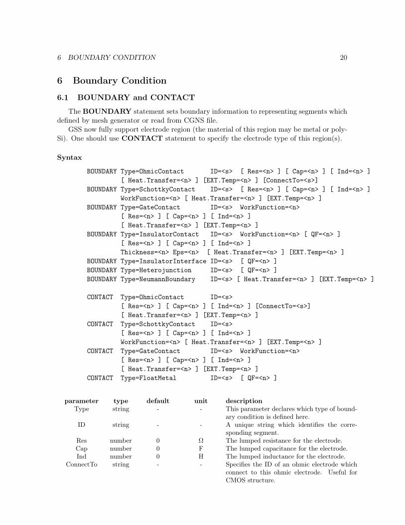
The BOUNDARY statement sets boundary information to representing segments whichdefined by mesh generator or read from CGNS file.
GSS now fully support electrode region (the material of this region may be metal or poly-Si). One should use CONTACT statement to specify the electrode type of this region(s).
parameter type default unit descriptionType string - - This parameter declares which type of bound-
ary condition is defined here.ID string - - A unique string which identifies the corre-
sponding segment.Res number 0 Ω The lumped resistance for the electrode.Cap number 0 F The lumped capacitance for the electrode.Ind number 0 H The lumped inductance for the electrode.
ConnectTo string - - Specifies the ID of an ohmic electrode whichconnect to this ohmic electrode. Useful forCMOS structure.
6 BOUNDARY CONDITION 21
WorkFunction number 4.7 V The workfunction of the Schottky contact orgate material.
QF number 0 C · cm−2 For InsulatorContact and InsulatorInter-face bc: The surface charge density ofsemiconductor-insulator interface.
QF number 0 C · cm−2 For Heterojunction bc: The surface chargedensity of heterojunction.
QF number 0 C · µm−1 For FloatMetal bc: The free charge per micronin Z dimension.
Thickness number 2e-7 cm The thickness of SiO2 layer.Eps number 3.9 - The relative permittivity of SiO2 layer.
Heat.Transfer number 1e3 W/(cm ·K) The heat transfer rate of boundary.EXT.Temp number LatticeTemp K The external temperature.
Four "electrode" boundary conditions are supported by GSS. The names are ended with"Contact". The OhmicContact and SchottkyContact electrodes have current flow in bothsteady state and transient situations. While GateContact and InsulatorContact(a simplifiedMOSFET Gate boundary condition) only have displacement current in transient situation.
GSS supports five interfaces which can be set automatically: semiconductor-insulatorinterface(InsulatorInterface), semiconductor-electrode interface(set to OhmicContract as de-fault), interface between different semiconductor material(Heterojunction) and interface be-tween same semiconductor material(Homojunction). These boundaries can be set automati-cally by GSS if user didn’t set them explicitly. However, the electrode-insulator interface,may have several situations: Gate to Oxide interface, FloatMetal to Oxide interface orSource/Drain electrode to Oxide interface. As a result, this interface can only be set correctlywhen electrode type is known. Please refer to the following CONTACT statement.
GSS can build region with metal or poly-Si material to form an electrode. Which means,i.e. for OhmicContact bc, one can simply specify a segment as Ohmic bc or build an electroderegion as Ohmic electrode. Since Version 0.45.03, GSS considers electrode region, semicon-ductor region and insulator region during calculation. As a result, GSS added CONTACTstatement for fast boundaries specification of electrode region. At present, GSS support elec-trode with the type of Ohmic, Schottky, Gate and FloatMetal. All the electrode should bespecified explicitly and GSS will set corresponding boundaries automatically.
6 BOUNDARY CONDITION 22
The "ID" parameter of BOUNDARY statement is limited to segment label. And The"ID" parameter of CONTACT statement is limited to region name.
The NeumannBoundary, which is the default boundary type for all the non-interfacesegments, can also be set automatically.
6 BOUNDARY CONDITION 23
6.2 ATTACH
This statement is used to add voltage or current sources to the electrode boundary. Thestatement first clears all the sources connected to the specified electrode and then addssource(s) defined by VApp or IApp parameter. If two or more sources are attached to thesame electrode, the total effect is the summation of all sources. However, the sources attachedto one electrode must have the same type.
parameter type default unit descriptionElectrode string - - Specifies which electrode boundary is to be at-
tached with one or more sources.Type string Voltage - The sources are voltage or current type.VApp string - - Specifies the ID of voltage source which is to
be attached to this electrode.IApp string - - Specifies the ID of current source which is to
If electrode is attached with voltage source(s), the R, C and L defined by BOUNDARYstatement will affect later simulation. But solver will ignore those lumped elements with theelectrode which stimulated by current source(s). Please refer to Fig 4.
The positive direction of current is flow into the electrode.Only Ohmic and Schottky electrodes can be attached by current source(s).If no source attached explicitly, the electrode is set to be attached to ground.
Figure 4: Voltage and current boundary.
7 PHYSICAL MODEL INTERFACE 24
7 Physical Model Interface
GSS use a dynamic mechanician to support various materials and physical models. Eachmaterial has a dynamic load library (.so) which contains its physical parameters. User canmodify the parameters which can be found at $(GSS_DIR)/src/material and recompile it.Experts can even offer their own physical model files.
At present, GSS has a PMIS statement for choosing different mobility models and impactionization models.
Syntax
PMIS Region=<s> Mobility=<s> II.Model=<s>
parameter type default unit descriptionRegion string - - Specifies the semiconductor region which use
the following physical model.Mobility string Analytic - The mobility model name.II.Model string Default - The impact ionization model name.
One can set different physical models to individual region.GSS has implemented Analytic, Philips and Lucent mobility model for all the supported
material. The Analytic and Philips mobility model only takes parallel field effect and they canbe used within all the four solvers. The author suggest to use these models for bipolar devicesimulations. The Lucent mobility model, which considers parallel and transverse electricalfield, is an accurate model for MOS structure. But it should work with DDML1E/DDML2Esolvers in which transverse electrical field is calculated. The Lombardi and HP (Hewlett-Packard) mobility model only validate for Silicon. These two mobility models include paralleland transverse electrical field corrections and can be used for MOSFET simulation. TheHypertang mobility model only validate for GaAs. It is reported that this model can avoidunrealistic drain current oscillation when applied to the simulation of GaAs MESFET.
The impact ionization model is still very limited in GSS. Only Valdinoci model for siliconis valid at present.
8 SOLVE SPECIFICATION 25
8 Solve Specification
8.1 Introduction
These statements instruct GSS core to perform user specified solution(s).
8.2 METHOD
The METHOD statement sets the solver and the parameters of the solver. Atpresent, GSS 0.4x has basic DDM solver(DDML1E), lattice temperature corrected DDMsolver(DDML2E) and EBML3E solver which base on energy balance model.
parameter type default unit descriptionType string DDML1 - Specifies the solver.
Scheme string Newton - At present, GSS only supports Newton’s fulliterative scheme.
HighFieldMobility bool On - Specifies if high field mobility should be used.GSS set this flag to OFF for equilibrium state.
EJModel bool Off - Specifies if EdotJ and EcrossJ should be useto calculate high field mobility. GSS will usea simpler model when this flag is set to OFF.
ImpactIonization bool Off - Specifies if impact ionization should be con-sidered.
II.Type string GradQf - Specifies the implement model of impact ion-ization.
BandBandTunneling string Off - Specifies if band to band tunneling should beconsidered.
Fermi bool Off - Specifies if Fermi-Dirac statistics should beconsidered.
NS string LineSearch - Specifies the nonlinear solver.LS string GMRES - Specifies the linear solver.
Damping string No - Load a Newton damping method for Line-Search or Basic Newton nonlinear solver.
8 SOLVE SPECIFICATION 26
MaxIteration integer 30 - The max number of iteration nonlinear solverwill try. But for equilibrium state calculation,the max allowed iteration number is 10 timesmore than this value.
relative.tol number 1e-5 - When relative error of solution variable lessthan this value, solution is considered con-verged.
possion.tol number 1e-26 C · µm−1 The absolute converged criteria for the Pois-son equation.
elec.continuty.tol number 5e-18 A · µm−1 The absolute converged criteria for the elec-tron continuity equation.
hole.continuty.tol number 5e-18 A · µm−1 The absolute converged criteria for the holecontinuity equation.
elec.energy.tol number 1e-18 W · µm−1 The absolute converged criteria for the elec-tron energy balance equation.
hole.energy.tol number 1e-18 W · µm−1 The absolute converged criteria for the holeenergy balance equation.
latt.temp.tol number 1e-11 W · µm−1 The absolute converged criteria for the latticeheat equation equation.
electrode.tol number 1e-9 V The absolute converged criteria for the elec-trode bias equation.
toler.relax number 1e4 - When relative error is used as converged crite-ria, the equation norm should satisfy the ab-solute converged criteria with a relaxation ofthis value.
QNFactor number 1.0 - The damping quantity of electron quantumpotential.
QPFactor number 1.0 - The damping quantity of hole quantum poten-tial.
All the DDML1E/DDML2E/EBML3E/QDDML1E solvers support parallel and trans-verse electrical field dependent mobility.
Lattice temperature equation is considered by DDML2E solver. The EBML3E solveris based on advanced energy balance method. The QDDML1E is a density-gradient solverwhich consists of quantum correction to classical model.
The carrier generation by impact ionization and band band tunneling is really difficult forcalculation. However, DDML1E/DDML2E solvers are carefully designed for impact ionizationand band band tunneling calculation, i.e. diode reverse breakdown simulation. Usually, thetemperature can’t keep unchanged if carrier generation takes place. As a result, DDML2Esolver is highly recommend for these types of situations. At present, EBML3E and QDDML1Esolver don’t support impact ionization.
8 SOLVE SPECIFICATION 27
Fermi statistics is only supported by DDML1E and DDML2E solvers.LineSearch and TrustRegion accelerating methods work well when initial value a bit far
from real solution, e.g. first time computing. Basic Newton method should only be usedwhen initial value is near the true solution, e.g. dc sweep and transient calculation.
Each nonlinear solver should have a inner linear solver. To choose a suitable linear solvermay help the convergence. The performance of LineSearch and Basic Newton methods isgood when Krylov subspace linear solvers(CGS, BICG, BCGS, GMRES and TFQMR) areemployed. However, the TrustRegion method prefers LU factorization linear solver to Krylovsubspace linear solvers.
Newton Damping is a useful tool for helping convergence, especially for the Basic Newtonmethod.
QNFactor and QPFactor is used to enforce the convergence property of QDDML1E solver.Since quantum solution differs much from classical solution near Si/SiO2 interface, settingthese two factors with small value i.e. 1e-4 and varying it gradually to 1.0, with each step thesolution can get convergence. At last, the value of QXFactor of 1.0 means that the quantummodel is fully turned on and applied.
The parameters of METHOD statement will not be affected by previous METHODstatement.
The convergence is considered to be achieved when either the X norm or the functionresidual norm falls below certain tolerance. When every function’s residual norm falls smallthan certain tolerance, the absolute convergence is achieved. For X norm criteria, it shouldfall below relative.tol and every function residual norm should fit the relaxed (with therelaxation value of toler.relax) absolute converged criteria.
8 SOLVE SPECIFICATION 28
8.3 SOLVE
The SOLVE statement instructs GSS to perform a solution for one or more specified biaspoints.
parameter type default unit descriptionType string - - Specifies the Solve condition.VScan string - - Specifies the voltage variational electrode
boundary for DCSWEEP.VStart number - V The initial voltage for DC sweep.VStep number - V The voltage step size of DC sweep.VStop number - V The finish voltage for DC sweep.IScan string - - Specifies the current variational electrode
boundary for DCSWEEP.IStart number - mA The initial current for DC sweep.IStep number - mA The current step size of DC sweep.IStop number - mA The finish current for DC sweep.
IV.Record string - - Specifies which electrode’s IV data should berecorded. User can define serval electrodeshere.
IV.File string - - Specifies the file which contains the IV data.ODE.Formula string BDF2 - Specifies the time march scheme for solving
the time-domain ordinary differential equa-tion.
TStart number - s The initial time for transient calculation.TStep number - s The time step size of transient calculation.TStop number - s The finish time for transient calculation.
AutoStep bool - True Use automatically time step control based onLTE.
Predict bool - True Predict initial value for next time step.
For equilibrium state calculation, all the electrodes are set to ground.You can’t do a DC sweep with current scan to GateContact and InsulatorContact.When STEADYSTATE or DCSWEEP solve is performed, transient 0 value of the volt-
age(current) source will be used as the bias of each electrode.One can do voltage DCSWEEP with multi-electrode by specifying two or more VScan
parameter. The voltage will be assigned to each electrode during the simulation. This functionis useful for Double Gate MOS simulation.
The step size for DCSWEEP calculation will automatically reduce to half size if last stepdiverged. Then it will be multiplied by 1.1 on each step until it reaches original step size.
TRANSIENT simulation now use automatically time step control based on LTE (localtruncation error).
8 SOLVE SPECIFICATION 30
8.4 AC Sweep Solver
In addition to DC steady state and transient analysis, GSS now allows AC small-signalanalysis as a post-processing step after a DC solution.
parameter type default unit descriptionACScan string - - Specifies the electrode for ACSWEEP.FStart number 1e6 Hz The initial frequency for AC sweep.
FMultiple number 1.1 - The multiplicative factor for incrementing fre-quency.
FStop number 1e9 Hz The finish frequency for AC sweep.VAC number 0.0026 V The magnitude of the applied small-signal
bias.
Hint
This solver shared Jacobian Matrix with DDML1E solver. Which means one should call itdirectly after DDML1E, keeping all the parameters unchanged for METHOD statement. Ifa previous computed result is imported, call DDML1E to do a steady-state calculation againand run DDML1AC later.
The convergence may be difficult if frequency is very high, i.e. nearly cut off frequency,because of the poor condition number of Jacobian matrix.
8 SOLVE SPECIFICATION 31
8.5 EM FEM Solver
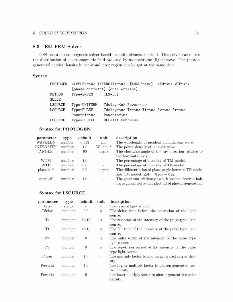
GSS has a electromagnetic solver based on finite element method. This solver calculatesthe distribution of electromagnetic field radiated by monochrome (light) wave. The photongenerated carrier density in semiconductor region can be got at the same time.
parameter type default unit descriptionWAVELEN number 0.532 µm The wavelength of incident monochrome wave.INTENSITY number 1.0 W · cm−2 The power density of incident wave.
ANGLE number 90 degree The clockwise angle of the ray direction relative tothe horizontal axis.
WTM number 1.0 - The percentage of intensity of TM model.WTE number 0.0 - The percentage of intensity of TE model.
phase.diff number 0.0 degree The differentiation of phase angle between TE modeland TM model. ∆Φ = ΦTM − ΦTE
quan.eff number 1.0 - The quantum efficiency (which means electron-holepares generated by one photon) of photon generation.
Syntax for LSOURCE
parameter type default unit descriptionType string - - The type of light source.
Tdelay number 0.0 s The delay time before the activation of the lightsource.
Tr number 1e-15 s The rise time of the intensity of the pulse-type lightsource.
Tf number 1e-15 s The fall time of the intensity of the pulse type lightsource.
Pw number 0 s The pulse width of the intensity of the pulse typelight source.
Pr number 0 s The repetition period of the intensity of the pulsetype light source.
Power number 1.0 - The multiply factor to photon generated carrier den-sity.
Powerhi number 1.0 - The higher multiply factor to photon generated car-rier density.
Powerlo number 0 - The lower multiply factor to photon generated carrierdensity.
8 SOLVE SPECIFICATION 32
DLL string - - The name of dynamic library file.Func string - - The name of the function loaded from dynamic li-
brary file which calculates power coefficient.
Hint
User need to build a vacuum region surrounding device and a PML region surroundingvacuum region. These two region should have a thickness of no less than one wave length.
The work flow of EMFEM solver shows as follows. GSS set its internal solver to EMFEMwhen meets METHOD command with EMFEM type. The actual solving action takes placewhen meets the next SOLVE command. GSS will search the first PHOTOGEN commandin the input list, using the parameters in this command during the solve procedure. ThisPHOTOGEN command will be removed from input list after solving action. As a result,user can set multi PHOTOGEN statements and repeat SOLVE command for correspondingtimes to calculate several beams of monochrome wave, during which the photon generatedcarrier density will be added to previous result.
The iterative method such as GMRES usually leads to divergence when solving FEMproblem. LU factorization is highly recommend.
EMFEM only gets the photon generated carrier density. User should set one LSOURCEto describe the time evolution of the light source. The actual photon generated carrier densityused in semiconductor simulation is the original value multiplied with power coefficientspecified within LSOURCE.
When DDML1E or DDML2E solver is loaded for further simulation, the photon generatedcarrier will be considered.
User can define their own light source by dynamic loaded library as voltage or currentsource. Here is a template.
foo.c:double lsrc_power(double time) /* in the unit of s */
double power;/* calculate the power of light source */return power;
8 SOLVE SPECIFICATION 33
8.6 IV File Format
GSS can generate IV record file for DC sweep, transient and AC sweep calculations. Hereis the file format for the three situations.
The file for DC sweep: The first line is begin with ’#’, followed by the name of eachelectrode. The remain part is the potential and current for each electrode, each takes onecolumn. The unit of potential is volt and the unit of current is mA.
The file for transient calculation is nearly the same as the file for DC sweep, besides thatthe first column is the time with the unit of ps.
The file for AC sweep has the same head as above. The remaining part is organized asfollows: The first column is the frequency with the unit of MHz. Then the IV properties ofeach electrode. Each electrode takes six columns, the real, image and amplitude of potential,followed by three columns for current.
Note: the electrode potential may not equal to the application voltage if lumped elementstake place.
9 FILE I/O 34
9 File I/O
9.1 Introduction
The IMPORT and EXPORT statements are used to read and write solutions from aCGNS or TIF file. A model CGNS file only contains semiconductor device structure whilea core CGNS file has previous solution data besides device structure. The TIF(TechnologyInterchange Format) file is an ASCII file used by Synopsys Medici software which equivalenceto core CGNS file. We offer a small code TIFTool which can open TIF file, view the meshand solution data and convert it to CGNS file.
VTK file is intended to be used for post process. User can use Paraview1, MayaVi orVisIt2 to open and view VTK file. Further more, CGNS file is also supported by VisIt.
parameter type default unit descriptionVariable string - - This parameter specifies plot context.PS.OUT string - - Specifies the postscript file name. The plot
window will be saved to it.TIFF.OUT string - - Specifies the TIFF file name. The plot window
will be saved to it. Only available for X11system.
Resolution string RES.Middle - The resolution of plot window.Measure string Linear Specifies the data axis to be linear or logarith-
mic.AzAngle number 240 degree The initial azimuthal rotation angle,
0≤AzAngle<360.ElAngle number 60 degree The initial elevation rotation angle.
PlotMesh is an interactive GUI for mesh display only exist for X11 system.The PLOT command can be used on both X11 and Win32 systems. The 3D plot can be
rotated by mouse and terminated by ESC key press. If PS.OUT or TIFF.OUT argument isspecified, the latest window image will be saved.
10 POST PROCESS 36
10.2 Probe
The PROBE statement is used to extract field data along a user defined segment. Thesegment can be a boundary or a segment pre-defined in the region. For the in-region segment,GSS will set it as Neumann boundary with no heat flux which takes not effect to simulationresult.
parameter type default unit descriptionVariable string - - This parameter specifies probe context.Region string - - Specifies the region name which the segment belongs to.
Segment string - - Specifies the segment name for probing the data.ProbeFile string - - The file name for recording the data.Append bool OFF - Specifies the data should be appended to the file.
Each PROBE statement records one variable for the whole segment to a user-specifiedfile. GSS pushes PROBE statement as the sequence of input text into a stack until a SOLVEstatement is met. These PROBE statements record the data during solve process. Afterthat, GSS will clear the stack. In short, PROBE only operates for next SOLVE process.
The head of file is the segment information, including region name, segment name, totalnode number and the location of each node. The last line of head shows the solve typeand variable name. The solve type can be "EQUILIBRIUM", "STEADYSTATE", "DC-SWEEP_VSCAN", "DCSWEEP_ISCAN" and "TRANSIENT". For the last three types,GSS will record V/I/Time in the first column, respectively. The variable value for all thenodes are listed in the same line.
11 CONVERGENCE PROBLEM 37
11 Convergence Problem
The core arithmetic of GSS is solving the large scale nonlinear equations arisen fromsemiconductor drift-diffusion model by Newton’s Iterative method. There are three factorswhich affect the convergence of nonlinear solvers: the initial value, the Jacobian Matrix andthe inner linear solver. One must ensure that the initial value is sufficiently near the realsolution, the Jacobian Matrix is exact or at least nearly exact and the inner linear solver cangive a suitable solution. When one of the three demands is not satisfied, the convergenceproblem may raise. However, several skills can help convergence.
If the first time running failed due to bad initial value, one can employ a transient solverto do a time evolved solution. Set time step to a few ps, and the solution on every step mayget convergence. After some certain steps, the initial shock is damped and physical variablesare forced to get close to real quantities. Then the steady-state solver may work and you canget the equilibrium solution.
Since version 0.46, GSS use automatically differentiation to calculate Jacobian matrix. Inmost situations, author can guarantee that Jacobian matrix is exact, except some rigoroussituations when round-off error is un-neglectable. However, GSS offers alternative choice, theMatrix-Free method to set Jacobian Matrix by finite difference approximation. This choicecan be invoked with the command line option -snes_mf_operator. The Matrix-Free methodworks well when impact ionization takes place, but it runs much slower than original method.
Sometimes the LineSearch method may failed due to bad search direction. If one getdivergence message during DC sweep and transient simulation when using LineSearch method,one can try TrustRegion or basic Newton method.
Newton damping is a powerful tool to help convergence. It can work with LineSearchand Basic Newton solvers. GSS has two damping method, BankRose and Potential. Usually,damping Potential is better than BankRose.
The most difficult problem is the failure of inner linear solver. When the Jacobian Matrixis singular, problems may happen. Especially one sets electrodes with lumped resistor orcurrent sources. If one get a convergence failed message for these situations, please check theproblem by adding command line option -ksp_monitor to exam the convergence history. Formore information, one can use -ksp_singmonitor to get the condition number of matrix (thisworks only with GMRES method).
The author suggests some method to overcome the problem. First, one may improvethe condition number by enlarging the DopingScale, but this will increase numerical error.Second, one should carefully choose the linear solver.
Here is the introduction of the main linear solvers GSS can use. GMRES is a robustmethod for non-symmetric matrices. It must retain all the previous vectors during iterative.The implemented code often uses a "restart" method to avoid large memory requirement.Sometimes the solution breaks when restart too often. One can increase this restart stepsby -ksp_gmres_restart <n> (n is the restart steps, default 150) BiCG and CGS often haveirregular convergence behavior. The irregular result may get things worse. Bi-CGSTAB isthe improved method to BiCG and CGS, which avoids the irregular convergence patternsof BiCG/CGS while maintaining about the same speed of convergence. TFQMR avoids theirregular convergence behavior of BiCG. Also it avoids some breakdown situations of BiCG.When BiCG temporarily stagnates or diverges, TFQMR may still works. At last, LU factor-
12 MEMORY AND CPU REQUIREMENT 38
ization is the basic method for solving linear systems. Besides build-in LU solver, PETSCcan be compiled with external LU factorization package such as SuperLU and UMFPACK.This method works slow but usually more stable than iteration solver.
In conclusion, LU factorization is recommend for conquering the singular problem. Butuser can try GMRES with large restart steps, Bi-CGSTAB and TFQMR methods for betterefficiency.
12 Memory and CPU requirement
Thanks to C++’s dynamic memory manege system, GSS can solve problems with any scale(at least, theoretically). The memory requirement is not a serious bottleneck. A very largeproblem which contains 100K nodes only requires about 300MB memory. This requirementis easy to be satisfied with modern computers.
Because the core arithmetic of GSS is solving nonlinear equations, which involves lots ofsolutions of linear system, the CPU time is related with linear solvers, which is O(n3) withLU solver and O(n2) with krylov iterative solver, in which n is the problem scale.
Fig5 shows the CPU time vs node number with a PN diode simulation by BCGS methodon a Xeon 3.6GHz workstation. The time is approximate the square of problem scale. It onlyrequires serial seconds when total node number less than 5000. But CPU time raises to someminutes when node’s number reach to 100K.
The purpose of this License is to make a manual, textbook, or other functional and usefuldocument “free” in the sense of freedom: to assure everyone the effective freedom to copyand redistribute it, with or without modifying it, either commercially or noncommercially.Secondarily, this License preserves for the author and publisher a way to get credit for theirwork, while not being considered responsible for modifications made by others.
This License is a kind of “copyleft”, which means that derivative works of the documentmust themselves be free in the same sense. It complements the GNU General Public License,which is a copyleft license designed for free software.
We have designed this License in order to use it for manuals for free software, because freesoftware needs free documentation: a free program should come with manuals providing thesame freedoms that the software does. But this License is not limited to software manuals; itcan be used for any textual work, regardless of subject matter or whether it is published as aprinted book. We recommend this License principally for works whose purpose is instructionor reference.
A.1 Applicability and definitions
This License applies to any manual or other work, in any medium, that contains a noticeplaced by the copyright holder saying it can be distributed under the terms of this License.Such a notice grants a world-wide, royalty-free license, unlimited in duration, to use thatwork under the conditions stated herein. The “Document”, below, refers to any such manualor work. Any member of the public is a licensee, and is addressed as “you”. You acceptthe license if you copy, modify or distribute the work in a way requiring permission undercopyright law.
A “Modified Version” of the Document means any work containing the Document or aportion of it, either copied verbatim, or with modifications and/or translated into anotherlanguage.
A “Secondary Section” is a named appendix or a front-matter section of the Documentthat deals exclusively with the relationship of the publishers or authors of the Documentto the Document’s overall subject (or to related matters) and contains nothing that couldfall directly within that overall subject. (Thus, if the Document is in part a textbook ofmathematics, a Secondary Section may not explain any mathematics.) The relationshipcould be a matter of historical connection with the subject or with related matters, or oflegal, commercial, philosophical, ethical or political position regarding them.
A GNU FREE DOCUMENTATION LICENSE 40
The “Invariant Sections” are certain Secondary Sections whose titles are designated, asbeing those of Invariant Sections, in the notice that says that the Document is released underthis License. If a section does not fit the above definition of Secondary then it is not allowedto be designated as Invariant. The Document may contain zero Invariant Sections. If theDocument does not identify any Invariant Sections then there are none.
The “Cover Texts” are certain short passages of text that are listed, as Front-Cover Textsor Back-Cover Texts, in the notice that says that the Document is released under this License.A Front-Cover Text may be at most 5 words, and a Back-Cover Text may be at most 25 words.
A “Transparent” copy of the Document means a machine-readable copy, represented ina format whose specification is available to the general public, that is suitable for revisingthe document straightforwardly with generic text editors or (for images composed of pixels)generic paint programs or (for drawings) some widely available drawing editor, and that issuitable for input to text formatters or for automatic translation to a variety of formatssuitable for input to text formatters. A copy made in an otherwise Transparent file formatwhose markup, or absence of markup, has been arranged to thwart or discourage subsequentmodification by readers is not Transparent. An image format is not Transparent if used forany substantial amount of text. A copy that is not “Transparent” is called “Opaque”.
Examples of suitable formats for Transparent copies include plain ASCII without markup,Texinfo input format, LATEX input format, SGML or XML using a publicly available DTD,and standard-conforming simple HTML, PostScript or PDF designed for human modification.Examples of transparent image formats include PNG, XCF and JPG. Opaque formats includeproprietary formats that can be read and edited only by proprietary word processors, SGMLor XML for which the DTD and/or processing tools are not generally available, and themachine-generated HTML, PostScript or PDF produced by some word processors for outputpurposes only.
The “Title Page” means, for a printed book, the title page itself, plus such following pagesas are needed to hold, legibly, the material this License requires to appear in the title page.For works in formats which do not have any title page as such, “Title Page” means the textnear the most prominent appearance of the work’s title, preceding the beginning of the bodyof the text.
A section “Entitled XYZ” means a named subunit of the Document whose title either isprecisely XYZ or contains XYZ in parentheses following text that translates XYZ in anotherlanguage. (Here XYZ stands for a specific section name mentioned below, such as “Acknowl-edgements”, “Dedications”, “Endorsements”, or “History”.) To “Preserve the Title” of sucha section when you modify the Document means that it remains a section “Entitled XYZ”according to this definition.
The Document may include Warranty Disclaimers next to the notice which states that thisLicense applies to the Document. These Warranty Disclaimers are considered to be includedby reference in this License, but only as regards disclaiming warranties: any other implicationthat these Warranty Disclaimers may have is void and has no effect on the meaning of thisLicense.
A GNU FREE DOCUMENTATION LICENSE 41
A.2 Verbatim copying
You may copy and distribute the Document in any medium, either commercially or non-commercially, provided that this License, the copyright notices, and the license notice sayingthis License applies to the Document are reproduced in all copies, and that you add no otherconditions whatsoever to those of this License. You may not use technical measures to ob-struct or control the reading or further copying of the copies you make or distribute. However,you may accept compensation in exchange for copies. If you distribute a large enough numberof copies you must also follow the conditions in section A.3.
You may also lend copies, under the same conditions stated above, and you may publiclydisplay copies.
A.3 Copying in quantity
If you publish printed copies (or copies in media that commonly have printed covers) ofthe Document, numbering more than 100, and the Document’s license notice requires CoverTexts, you must enclose the copies in covers that carry, clearly and legibly, all these CoverTexts: Front-Cover Texts on the front cover, and Back-Cover Texts on the back cover. Bothcovers must also clearly and legibly identify you as the publisher of these copies. The frontcover must present the full title with all words of the title equally prominent and visible.You may add other material on the covers in addition. Copying with changes limited to thecovers, as long as they preserve the title of the Document and satisfy these conditions, canbe treated as verbatim copying in other respects.
If the required texts for either cover are too voluminous to fit legibly, you should put thefirst ones listed (as many as fit reasonably) on the actual cover, and continue the rest ontoadjacent pages.
If you publish or distribute Opaque copies of the Document numbering more than 100,you must either include a machine-readable Transparent copy along with each Opaque copy,or state in or with each Opaque copy a computer-network location from which the generalnetwork-using public has access to download using public-standard network protocols a com-plete Transparent copy of the Document, free of added material. If you use the latter option,you must take reasonably prudent steps, when you begin distribution of Opaque copies inquantity, to ensure that this Transparent copy will remain thus accessible at the stated lo-cation until at least one year after the last time you distribute an Opaque copy (directly orthrough your agents or retailers) of that edition to the public.
It is requested, but not required, that you contact the authors of the Document wellbefore redistributing any large number of copies, to give them a chance to provide you withan updated version of the Document.
A.4 Modifications
You may copy and distribute a Modified Version of the Document under the conditions ofsections A.2 and A.3 above, provided that you release the Modified Version under precisely thisLicense, with the Modified Version filling the role of the Document, thus licensing distributionand modification of the Modified Version to whoever possesses a copy of it. In addition, youmust do these things in the Modified Version:
A GNU FREE DOCUMENTATION LICENSE 42
A. Use in the Title Page (and on the covers, if any) a title distinct from that of theDocument, and from those of previous versions (which should, if there were any, belisted in the History section of the Document). You may use the same title as a previousversion if the original publisher of that version gives permission.
B. List on the Title Page, as authors, one or more persons or entities responsible forauthorship of the modifications in the Modified Version, together with at least five ofthe principal authors of the Document (all of its principal authors, if it has fewer thanfive), unless they release you from this requirement.
C. State on the Title page the name of the publisher of the Modified Version, as thepublisher.
D. Preserve all the copyright notices of the Document.
E. Add an appropriate copyright notice for your modifications adjacent to the other copy-right notices.
F. Include, immediately after the copyright notices, a license notice giving the publicpermission to use the Modified Version under the terms of this License, in the formshown in the Addendum below.
G. Preserve in that license notice the full lists of Invariant Sections and required CoverTexts given in the Document’s license notice.
H. Include an unaltered copy of this License.
I. Preserve the section Entitled “History”, Preserve its Title, and add to it an item statingat least the title, year, new authors, and publisher of the Modified Version as givenon the Title Page. If there is no section Entitled “History” in the Document, createone stating the title, year, authors, and publisher of the Document as given on itsTitle Page, then add an item describing the Modified Version as stated in the previoussentence.
J. Preserve the network location, if any, given in the Document for public access to aTransparent copy of the Document, and likewise the network locations given in theDocument for previous versions it was based on. These may be placed in the “History”section. You may omit a network location for a work that was published at least fouryears before the Document itself, or if the original publisher of the version it refers togives permission.
K. For any section Entitled “Acknowledgements” or “Dedications”, Preserve the Title of thesection, and preserve in the section all the substance and tone of each of the contributoracknowledgements and/or dedications given therein.
L. Preserve all the Invariant Sections of the Document, unaltered in their text and in theirtitles. Section numbers or the equivalent are not considered part of the section titles.
M. Delete any section Entitled “Endorsements”. Such a section may not be included in theModified Version.
A GNU FREE DOCUMENTATION LICENSE 43
N. Do not retitle any existing section to be Entitled “Endorsements” or to conflict in titlewith any Invariant Section.
O. Preserve any Warranty Disclaimers.
If the Modified Version includes new front-matter sections or appendices that qualify asSecondary Sections and contain no material copied from the Document, you may at youroption designate some or all of these sections as invariant. To do this, add their titles tothe list of Invariant Sections in the Modified Version’s license notice. These titles must bedistinct from any other section titles.
You may add a section Entitled “Endorsements”, provided it contains nothing but endorse-ments of your Modified Version by various parties–for example, statements of peer review orthat the text has been approved by an organization as the authoritative definition of a stan-dard.
You may add a passage of up to five words as a Front-Cover Text, and a passage of up to25 words as a Back-Cover Text, to the end of the list of Cover Texts in the Modified Version.Only one passage of Front-Cover Text and one of Back-Cover Text may be added by (orthrough arrangements made by) any one entity. If the Document already includes a covertext for the same cover, previously added by you or by arrangement made by the same entityyou are acting on behalf of, you may not add another; but you may replace the old one, onexplicit permission from the previous publisher that added the old one.
The author(s) and publisher(s) of the Document do not by this License give permission touse their names for publicity for or to assert or imply endorsement of any Modified Version.
A.5 Combining documents
You may combine the Document with other documents released under this License, underthe terms defined in section A.4 above for modified versions, provided that you include in thecombination all of the Invariant Sections of all of the original documents, unmodified, andlist them all as Invariant Sections of your combined work in its license notice, and that youpreserve all their Warranty Disclaimers.
The combined work need only contain one copy of this License, and multiple identicalInvariant Sections may be replaced with a single copy. If there are multiple Invariant Sectionswith the same name but different contents, make the title of each such section unique byadding at the end of it, in parentheses, the name of the original author or publisher of thatsection if known, or else a unique number. Make the same adjustment to the section titles inthe list of Invariant Sections in the license notice of the combined work.
In the combination, you must combine any sections Entitled “History” in the variousoriginal documents, forming one section Entitled “History”; likewise combine any sectionsEntitled “Acknowledgements”, and any sections Entitled “Dedications”. You must delete allsections Entitled “Endorsements”.
A.6 Collections of documents
You may make a collection consisting of the Document and other documents releasedunder this License, and replace the individual copies of this License in the various documents
A GNU FREE DOCUMENTATION LICENSE 44
with a single copy that is included in the collection, provided that you follow the rules of thisLicense for verbatim copying of each of the documents in all other respects.
You may extract a single document from such a collection, and distribute it individuallyunder this License, provided you insert a copy of this License into the extracted document,and follow this License in all other respects regarding verbatim copying of that document.
A.7 Aggregation with independent works
A compilation of the Document or its derivatives with other separate and independentdocuments or works, in or on a volume of a storage or distribution medium, is called an“aggregate” if the copyright resulting from the compilation is not used to limit the legal rightsof the compilation’s users beyond what the individual works permit. When the Documentis included in an aggregate, this License does not apply to the other works in the aggregatewhich are not themselves derivative works of the Document.
If the Cover Text requirement of section A.3 is applicable to these copies of the Document,then if the Document is less than one half of the entire aggregate, the Document’s Cover Textsmay be placed on covers that bracket the Document within the aggregate, or the electronicequivalent of covers if the Document is in electronic form. Otherwise they must appear onprinted covers that bracket the whole aggregate.
A.8 Translation
Translation is considered a kind of modification, so you may distribute translations of theDocument under the terms of section A.4. Replacing Invariant Sections with translationsrequires special permission from their copyright holders, but you may include translations ofsome or all Invariant Sections in addition to the original versions of these Invariant Sections.You may include a translation of this License, and all the license notices in the Document, andany Warranty Disclaimers, provided that you also include the original English version of thisLicense and the original versions of those notices and disclaimers. In case of a disagreementbetween the translation and the original version of this License or a notice or disclaimer, theoriginal version will prevail.
If a section in the Document is Entitled “Acknowledgements”, “Dedications”, or “History”,the requirement (section A.4) to Preserve its Title (section A.1) will typically require changingthe actual title.
A.9 Termination
You may not copy, modify, sublicense, or distribute the Document except as expresslyprovided for under this License. Any other attempt to copy, modify, sublicense or distributethe Document is void, and will automatically terminate your rights under this License. How-ever, parties who have received copies, or rights, from you under this License will not havetheir licenses terminated so long as such parties remain in full compliance.
A GNU FREE DOCUMENTATION LICENSE 45
A.10 Future revisions of this license
The Free Software Foundation may publish new, revised versions of the GNU FreeDocumentation License from time to time. Such new versions will be similar in spirit tothe present version, but may differ in detail to address new problems or concerns. Seehttp://www.gnu.org/copyleft/.
Each version of the License is given a distinguishing version number. If the Documentspecifies that a particular numbered version of this License “or any later version” applies to it,you have the option of following the terms and conditions either of that specified version or ofany later version that has been published (not as a draft) by the Free Software Foundation. Ifthe Document does not specify a version number of this License, you may choose any versionever published (not as a draft) by the Free Software Foundation.
Addendum: how to use this license for your documents
To use this License in a document you have written, include a copy of the License in thedocument and put the following copyright and license notices just after the title page:
If you have Invariant Sections, Front-Cover Texts and Back-Cover Texts, replace the“with...Texts.” line with this:
with the Invariant Sections being LIST THEIR TITLES, with the Front-Cover Textsbeing LIST, and with the Back-Cover Texts being LIST.
If you have Invariant Sections without Cover Texts, or some other combination of thethree, merge those two alternatives to suit the situation.
If your document contains nontrivial examples of program code, we recommend releasingthese examples in parallel under your choice of free software license, such as the GNU GeneralPublic License, to permit their use in free software.