28
Guidance on Measurement Elaboration and Examples
| Date post: | 31-Dec-2015 |
| Category: |
Documents |
| Upload: | elwin-ball |
| View: | 226 times |
| Download: | 0 times |

Guidance on Measurement
Elaboration and Examples

Central principle of C and GHG accounting
Emissions rate = “Activity” ☓ “Emission factor”

Central principle of C and GHG accounting
Emissions rate = “Activity” ☓ “Emission factor”
What is being done
E.g. • Area being planted to trees• Amount of fertilizer applied• Number of dairy cattle
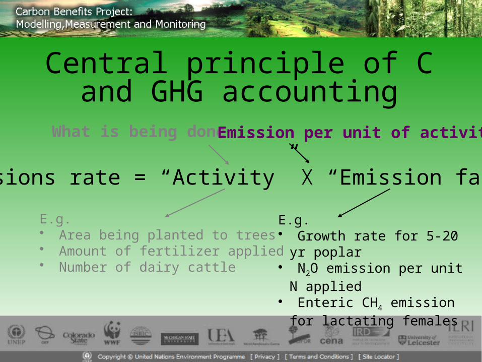
Central principle of C and GHG accounting
Emissions rate = “Activity” ☓ “Emission factor”
What is being done
E.g. • Area being planted to trees• Amount of fertilizer applied• Number of dairy cattle
Emission per unit of activity
E.g. • Growth rate for 5-20 yr poplar• N2O emission per unit N
applied• Enteric CH4 emission for
lactating females

Stratification• Activities are stratified (subdivided)
according to factors that most affect GHG emission rates/C sequestration rates
• Example for soil C stock changes– Cropland area is subdivided by:
• type of vegetation (grass vs crop), • relative productivity (fertilized vs non-fertilized), • plant residues (removed vs retained), • tillage type (intensity of soil disturbance)• etc.

Soil C stocks
C inputs
CO2
C losses
Example – factors determining soil C change
Variables in stock change factorsVegetation typeProductivityResidue managementManure additions
Soil type DrainageTillage
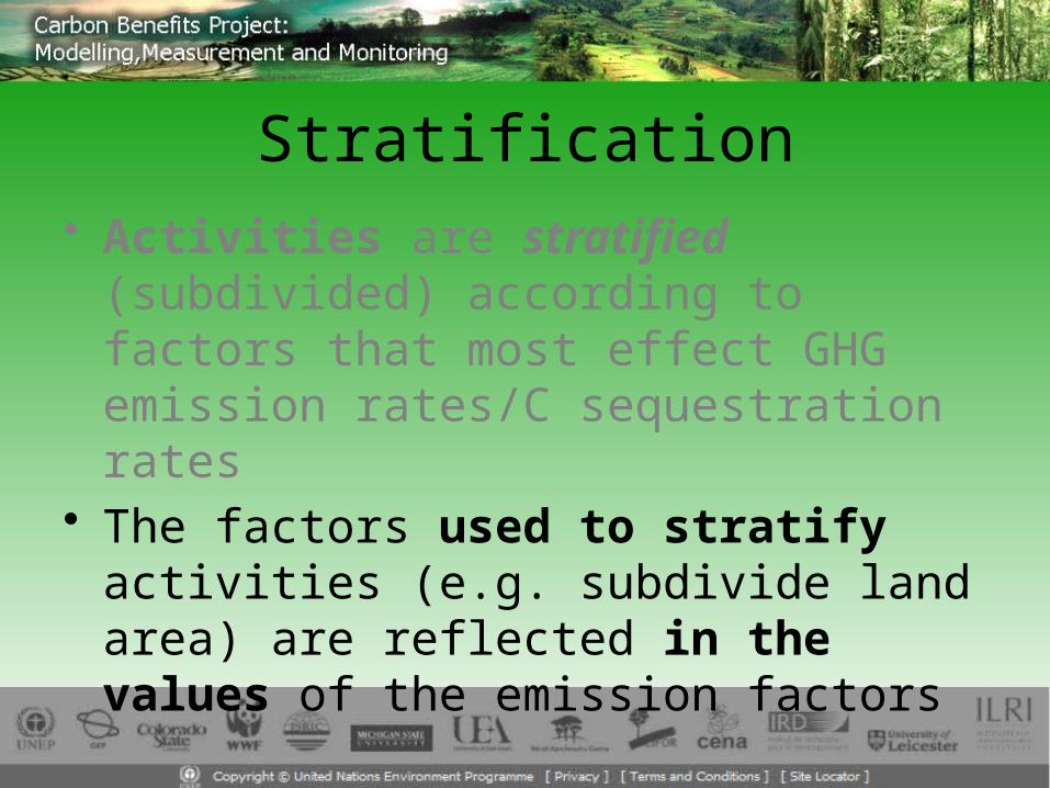
Stratification• Activities are stratified (subdivided)
according to factors that most effect GHG emission rates/C sequestration rates
• The factors used to stratify activities (e.g. subdivide land area) are reflected in the values of the emission factors

Simple example - Stock change factors for soil C
Δsoil C stocks = f (SOCref, Flu, Fi, Fm) for different climate and soil types
Climate/tillage type Conv.tillage
Reduced tillage
No-till
Temperate – dry 1 1.02 1.1
Temperate - moist 1 1.08 1.15
Tropical - dry 1 1.09 1.17
Tropical - moist 1 1.15 1.22
Values for Fm in Simple Assessment

Impact of Method used on stratification of activity data
Simple assessment• Emission & stock change factors are default values
supplied by the tool (cannot be changed)• Therefore, the stratification requirements for activity
data are already defined!
Thus the only data needed for GHG estimates are the stratified activity data (i.e., the area associated with each specified management system). But stratification needs to be consistent with the default factor definitions!
Collecting Activity Data• Participatory Rural Appraisal
– Most accurate and comprehensive– Requires good sampling design– Can be expensive

Collecting Activity Data• Participatory Rural Appraisal
– Most accurate and comprehensive– Requires good sampling design– Can be expensive
• Remote sensing– Appropriate for land cover changes (e.g. afforestation
area change)– Most management activities cannot be remotely-
sensed
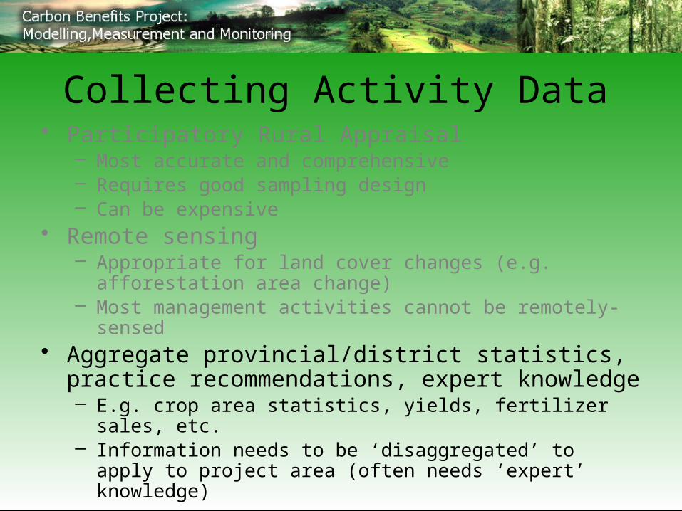
Collecting Activity Data• Participatory Rural Appraisal
– Most accurate and comprehensive– Requires good sampling design– Can be expensive
• Remote sensing– Appropriate for land cover changes (e.g. afforestation area
change)– Most management activities cannot be remotely-sensed
• Aggregate provincial/district statistics, practice recommendations, expert knowledge– E.g. crop area statistics, yields, fertilizer sales, etc.– Information needs to be ‘disaggregated’ to apply to project area
(often needs ‘expert’ knowledge)

Impact of Method used on stratification of activity data
Simple assessment• Emission & stock change factors are default values
supplied by the tool• Therefore, the stratification requirements for activity
data are already set!
Detailed assessment
• Emission & stock change factors can be changed to project- or region-specific values.
• Project- or region-specific values need to be measured• Activity data may be stratified differently to coincide with
the project-specific emission (or stock change) factors!
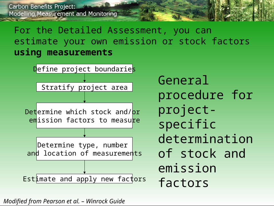
For the Detailed Assessment, you can estimate your own emission or stock factors using measurements
Define project boundaries
Stratify project area
Determine which stock and/or emission factors to measure
Determine type, number and location of measurements
Estimate and apply new factors
Modified from Pearson et al. – Winrock Guide
General procedure for project-specific determination of stock and emission factors
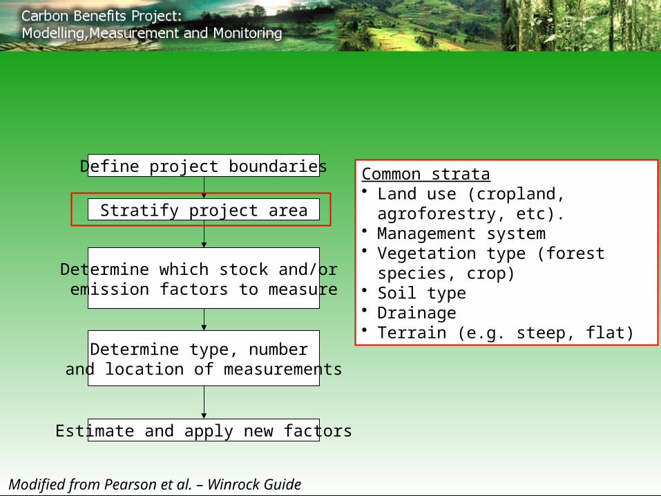
Define project boundaries
Stratify project area
Determine which stock and/or emission factors to measure
Determine type, number and location of measurements
Estimate and apply new factors
Modified from Pearson et al. – Winrock Guide
Common strata• Land use (cropland, agroforestry,
etc).• Management system• Vegetation type (forest species, crop)• Soil type• Drainage• Terrain (e.g. steep, flat)
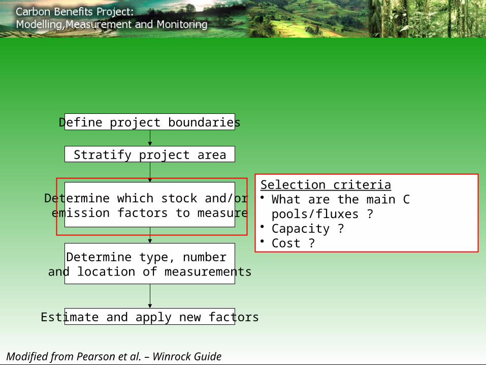
Define project boundaries
Stratify project area
Determine which stock and/or emission factors to measure
Determine type, number and location of measurements
Estimate and apply new factors
Modified from Pearson et al. – Winrock Guide
Selection criteria• What are the main C pools/fluxes ?• Capacity ?• Cost ?
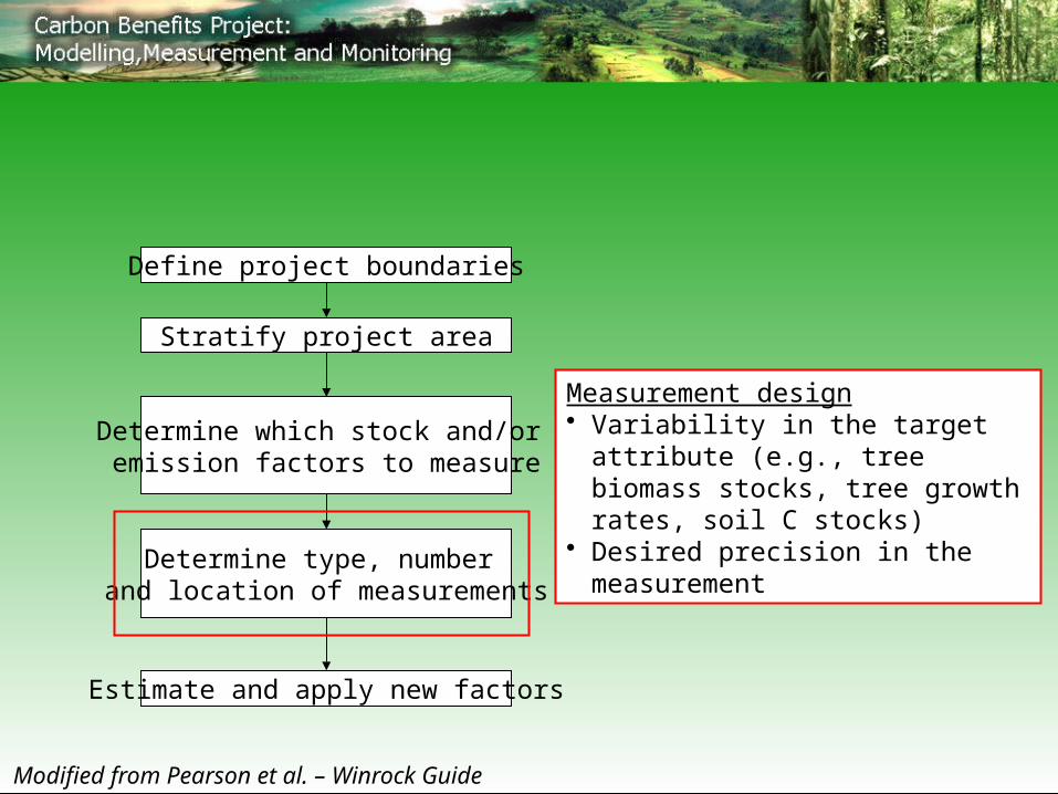
Define project boundaries
Stratify project area
Determine which stock and/or emission factors to measure
Determine type, number and location of measurements
Estimate and apply new factors
Modified from Pearson et al. – Winrock Guide
Measurement design• Variability in the target attribute (e.g.,
tree biomass stocks, tree growth rates, soil C stocks)
• Desired precision in the measurement

Example: Biomass C Losses from Deforestation
Ldf = A * (Bwp – Bwr) * (1+R) * CF *CO2-C
1) Forest area was stratified into two species/age groupsPines – 2000 haHardwoods – 1000 ha
2) Determine your sample requirements a) Get preliminary estimate of mean biomass and variability for these types of forests
- from literature or forest statistics- from a few preliminary plot measurements
Pines: mean = 100 t C/ha, SD = 15 t C/haHardwoods: mean = 80 t C/ha, SD = 25t C/ha

Example: Biomass C Losses from Deforestation
2) Determine your sample requirements b) plot numbers needed for desired precision
n = [(t * SD)/(m * p)]2
n – number of plotst – ‘t statistic’ (use t=2 for 95% CI)m - meanSD – standard deviationp – desired precision (e.g. use 0.1)
Pines: mean = 100 t C/ha, SD = 15 t C/haHardwoods: mean = 80 t C/ha, SD = 25t C/ha
How many plots needed for each forest type?
9 plots for the pines, 39 for the hardwoods

Example: Biomass C Losses from Deforestation
3) Establish plotsrandom vs griddedpermanent (fixed location)plot size and shape
4) Make measurements• typical tree measurements – diameter, height, crown density, etc.• For C inventory, use allometric equations to convert to biomass e.g. biomass per tree = f (dbh, height, basal area)

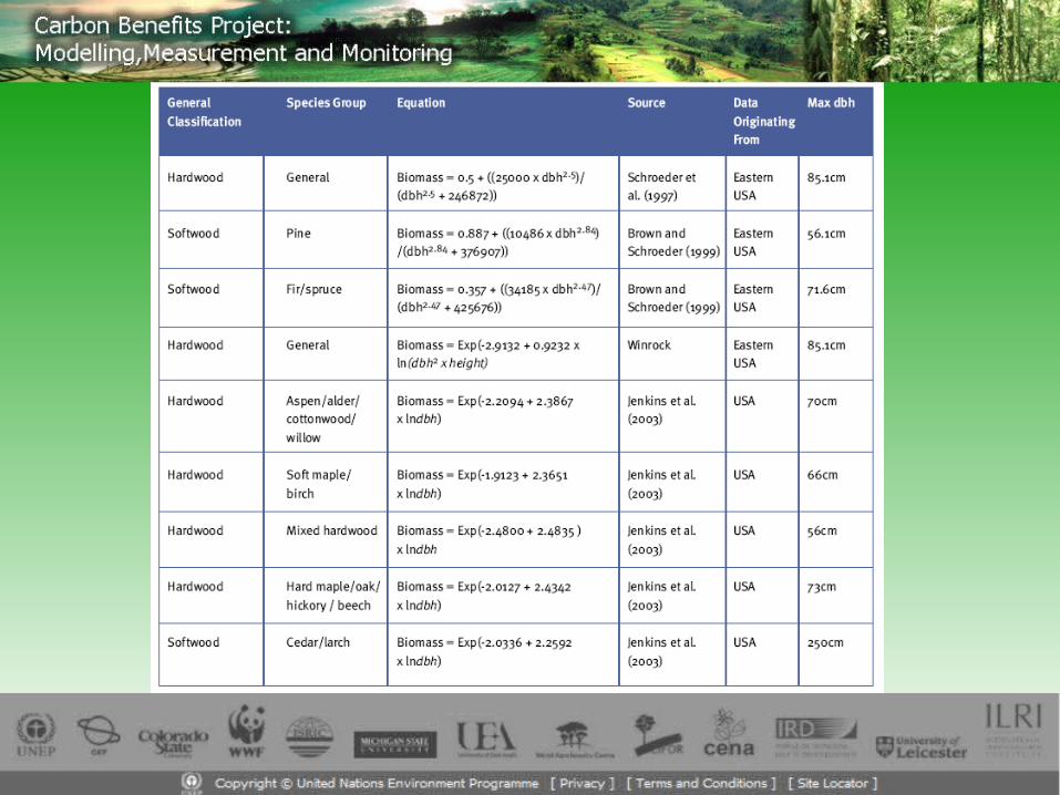

5) Estimate per tree biomass for each plot and sum biomass total for each plot
6) Compute mean and SD and apply expansion factor to scale from plot size to per ha
e.g. plot size = 100 m2, expansion factor = 100
7) Convert biomass units to C (e.g. default factor=2)
8) You’ve now derived your site specific value for ‘Bwp’ !
Ldf = A * (Bwp – Bwr) * (1+R) * CF *CO2-C
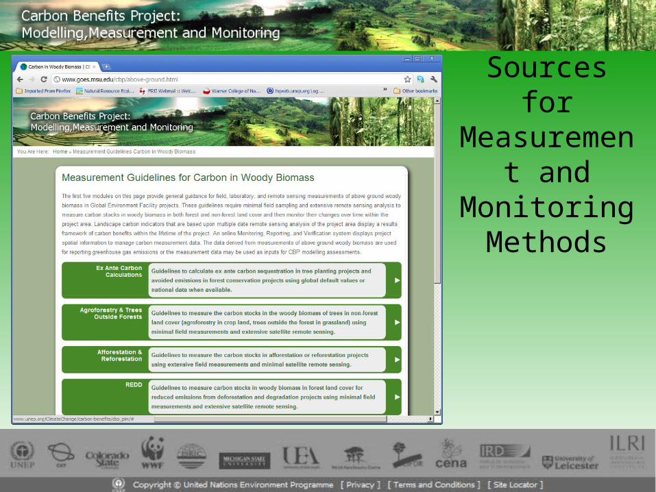
Sources for Measurement
and Monitoring Methods
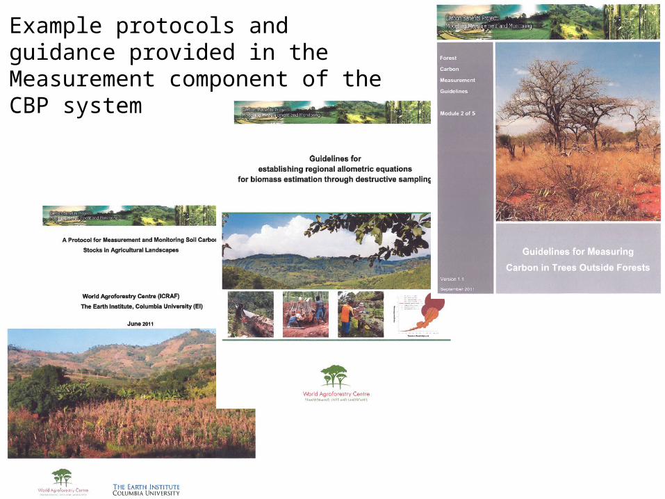
Example protocols and guidance provided in the Measurement component of the CBP system
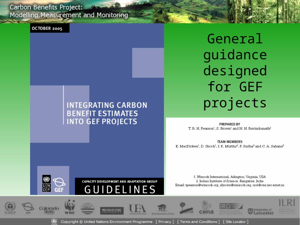
General guidance
designed for GEF projects

General Sources for Measurement and Monitoring
Methods

More Questions?
Obrigado!


