Page 1
Guide for customized SPEC macros at theSurface Diffraction StationX04SA Materials Science beamline,Swiss Light Source
written by
P.R. Willmott and C.M. Schleputz
Swiss Light Source
Paul Scherrer Institut
CH-5232 Villigen
Version 1.02
October 2006
Page 3
Contents
1 Introduction 1
1.1 Conventions . . . . . . . . . . . . . . . . . . . . . . . . . . . . . . . . . . . . . . . . . . . . . . . . 1
2 Getting started 3
2.1 Starting up SPEC . . . . . . . . . . . . . . . . . . . . . . . . . . . . . . . . . . . . . . . . . . . . 3
2.2 Getting help . . . . . . . . . . . . . . . . . . . . . . . . . . . . . . . . . . . . . . . . . . . . . . . . 4
2.3 Setting up an experiment . . . . . . . . . . . . . . . . . . . . . . . . . . . . . . . . . . . . . . . . 4
3 Site specific SPEC modifications 7
4 Movements, adjustments, and manipulations 9
4.1 The diffractometer . . . . . . . . . . . . . . . . . . . . . . . . . . . . . . . . . . . . . . . . . . . . 9
4.2 MOVE commands . . . . . . . . . . . . . . . . . . . . . . . . . . . . . . . . . . . . . . . . . . . . 9
4.3 HEXAPOD commands . . . . . . . . . . . . . . . . . . . . . . . . . . . . . . . . . . . . . . . . . . 11
5 Beam handling and security macros 15
5.1 FAST SHUTTER commands . . . . . . . . . . . . . . . . . . . . . . . . . . . . . . . . . . . . . . 15
5.2 DETECTOR SHUTTER commands . . . . . . . . . . . . . . . . . . . . . . . . . . . . . . . . . . 16
5.3 BEAM BLOCKER commands . . . . . . . . . . . . . . . . . . . . . . . . . . . . . . . . . . . . . 17
6 Filter and exposure settings 19
6.1 FILTER commands . . . . . . . . . . . . . . . . . . . . . . . . . . . . . . . . . . . . . . . . . . . 19
6.2 AUTO commands . . . . . . . . . . . . . . . . . . . . . . . . . . . . . . . . . . . . . . . . . . . . 21
7 Area detector macros 23
7.1 PIXEL commands . . . . . . . . . . . . . . . . . . . . . . . . . . . . . . . . . . . . . . . . . . . . 23
7.2 CCD commands . . . . . . . . . . . . . . . . . . . . . . . . . . . . . . . . . . . . . . . . . . . . . 26
7.3 IMAGE commands . . . . . . . . . . . . . . . . . . . . . . . . . . . . . . . . . . . . . . . . . . . . 26
8 Reciprocal space commands 29
8.1 Preparatory commands . . . . . . . . . . . . . . . . . . . . . . . . . . . . . . . . . . . . . . . . . 29
8.2 Orientation matrix commands . . . . . . . . . . . . . . . . . . . . . . . . . . . . . . . . . . . . . . 32
–iii–
Page 4
iv CONTENTS
8.3 Move and scan commands . . . . . . . . . . . . . . . . . . . . . . . . . . . . . . . . . . . . . . . . 36
8.4 Calculation commands . . . . . . . . . . . . . . . . . . . . . . . . . . . . . . . . . . . . . . . . . . 38
9 Sundry commands 41
9.1 Plotting commands . . . . . . . . . . . . . . . . . . . . . . . . . . . . . . . . . . . . . . . . . . . . 41
9.2 SMS commands . . . . . . . . . . . . . . . . . . . . . . . . . . . . . . . . . . . . . . . . . . . . . . 43
Index 46
Page 5
Chapter 1
Introduction
This document describes the functionality of SPEC macros customized for use at the Surface Diffraction station
of the Materials Science Beamline (MSBL) at the Swiss Light Source. These are included in our own flavours of
SPEC, called x04v and x04h , used for the Newport Micro-Controle surface diffractometer in so-called vertical
and horizontal geometries, respectively. “Standard” SPEC functions such as ascan, mesh, ct, etc., are produced
by standard.mac and are not described here (they can be found in the SPEC standard macro guide, either on
line or in a folder at the beamline). General tailoring of SPEC to the needs of the Materials Science beamline is
achieved automatically when starting up x04v or x04h , by invoking site_f.mac. The most important aspects
of site_f.mac are briefly described in Chapter 3.
1.1 Conventions
To use this document efficiently, there are some conventions one should be aware of.
1. Shell commands and prompts in SPEC are written in the typewriter style and highlighted in green;
2. SPEC macro names and arguments are written in the typewriter style. The macro name is highlighted
in blue, the argument(s) in red;
3. variable arguments are denoted by being surrounded by bra-ket brackets,
e.g., mvhkl <h> <k> <l>;
4. fixed (non-variable) arguments are identified by having no bracketing;
5. Optional arguments are surrounded by square brackets, e.g. [auto] in the command smsOn [auto];
6. The capitalization of macro names informs the user of their provenance: macro names with no underscores,
but capitalized first letters of concatenated words (e.g., autoSetLevel) are customized macros. As this
document primarily describes these macros, most of these follow this convention. The exception to this are
help macros (e.g., movehelp). These keep the lower case format (i.e., the “h” in movehelp) to maintain
–1–
Page 6
2 INTRODUCTION
consistency with standard help macros. Nonetheless, typing in e.g., moveHelp or indeed helpMove or
helpmove will call up movehelp, as an aid to (lack of) memory.
Any macros containing undescores or noncapitalized concatentated-word macro names originate from
standard.mac or the site-specific macro site.mac.
Page 7
Chapter 2
Getting started
2.1 Starting up SPEC
When a user begins experiments at the Surface Diffraction (SD) station of the Materials Science beamline
(MSBL), and assuming he/she will use SPEC and the customized commands described in this document, it is
important that he/she begins with a new SPEC file and that any unknown redefinitions of macros by previous
users have been removed. In order to start with such a fresh SPEC setup, open a shell and type in
[bash SLSBASE=/work]$ x04v -f
or
[bash SLSBASE=/work]$ x04h -f
depending on whether the vertical or horizontal geometry is being used (sse also Fig. 4.1). The -f option of the
command instructs SPEC to make a fresh start, which, in particular, involves reading the site_f.mac macro,
in which all the customized macros are embedded. Any information not included when calling x04v -f or
x04h -f (for example, macros created and implemented by a previous user), will be lost. Hence, any macros
previously written by the user which he/she would like to include should be qdo’d only after calling x04v -f
or x04h -f .
If for any reason, the user exits SPEC during the experiment, he/she should re-enter SPEC again using the
command
[bash SLSBASE=/work]$ x04v
or
[bash SLSBASE=/work]$ x04h
i.e., not calling a fresh startup of SPEC, by omitting the -f suffix. In this case, SPEC calls site.mac , which
is presently empty – in other words, no changes to SPEC are made.
–3–
Page 8
4 GETTING STARTED
2.2 Getting help
All standard SPEC commands or macros are described in detail in the SPEC manual. A printed version of
this can be found at the beamline, while a (questionably more updated) electronic version can be found at the
Certified Scientific Software (CSS) website http://www.certif.com/spec_manual/idx.html
To obtain more information of customized SPEC functionalities at the SD station, type in
sdhelp : Displays help topics.
Displays help topics specifically related to the SPEC setup at the Surface Diffraction Station of
the Materials Science Beamline X04SA at the Swiss Light Source (SLS). Detailed help texts of any
given topic can be called up by typing in the associated number.
2.3 Setting up an experiment
Before important experimental data begins 1, the user should call the macro
sdStartup : Sets up various filenames, directories, and crystallographic parameters at the start of an
experiment.
This command creates a logical directory tree, filenames, etc. Because of the importance of this
command, we describe it in more detail below.
Some explanations of the prompts and questions as they appear in sdStartup are now listed
1. Are you using an e-account? Reply with yes or no. Default is no. If your reply is yes, then the
following prompt will appear:
2. Please enter your e-account name Note that e-account numbers generally have the format e*****,
i.e., e followed by 5 digits.
3. Please enter a name for your project’s data directory, ending with the current date
in the following format: _yyyymmdd (e.g., Ni111_20050226) The example given is therefore for
work performed on the surface of Ni(111) starting on the 26th February 2005. This format is strongly
encouraged, for reasons of consistency.
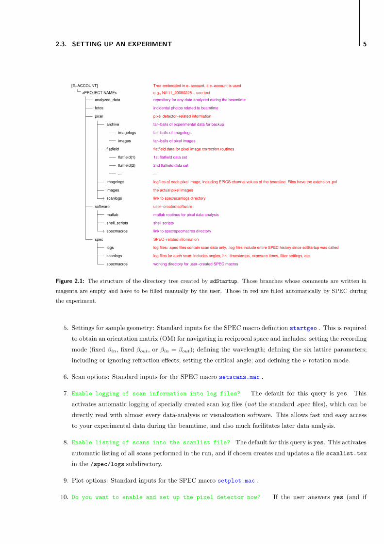
With this information, sdStartup then sets up for the user a project directory tree (each level is ordered
alphabetically). The structure of the tree is shown in Fig. 2.1.
4. Title for the scan headers, counting times, and update intervals: Standard inputs, normally requiring
simple confirmation by pressing return.
1The perception of what constitutes “important” experimental data is, needless to say, different from user to user. Some users
insist on knowing exactly what actions have been taken from opening the hutch door for the first time, while others might not want
their SPEC file to be cluttered with rudimentary alignment procedures – you choose. . .
Page 9
2.3. SETTING UP AN EXPERIMENT 5
[E−ACCOUNT]<PROJECT NAME>
analyzed_data
fotos
pixel
archive
flatfield
flatfield(1)
flatfield(2)
...
imagelogs
images
scanlogs
software
specmacros
spec
scanlogs
specmacros
logs
shell_scripts
matlab
pixel detector−related information
repository for any data analyzed during the beamtime
incidental photos related to beamtime
tar−balls of experimental data for backup
flatfield data for pixel image correction routines
2nd flatfield data set
1st flatfield data set
logfiles of each pixel image, including EPICS channel values of the beamline. Files have the extension .pxl
the actual pixel images
link to spec/scanlogs directory
user−created software
matlab routines for pixel data analysis
shell scripts
link to spec/specmacros directory
...
working directory for user−created SPEC macros
SPEC−related information
log files for each scan: includes angles, hkl, timestamps, exposure times, filter settings, etc.
log files: .spec files contain scan data only, .log files include entire SPEC history since sdStartup was called
Tree embedded in e−account, if e−account is usede.g., Ni111_20050226 − see text
images
imagelogs
tar−balls of pixel images
tar−balls of imagelogs
Figure 2.1: The structure of the directory tree created by sdStartup. Those branches whose comments are written in
magenta are empty and have to be filled manually by the user. Those in red are filled automatically by SPEC during
the experiment.
5. Settings for sample geometry: Standard inputs for the SPEC macro definition startgeo . This is required
to obtain an orientation matrix (OM) for navigating in reciprocal space and includes: setting the recording
mode (fixed βin, fixed βout, or βin = βout); defining the wavelength; defining the six lattice parameters;
including or ignoring refraction effects; setting the critical angle; and defining the ν-rotation mode.
6. Scan options: Standard inputs for the SPEC macro setscans.mac .
7. Enable logging of scan information into log files? The default for this query is yes. This
activates automatic logging of specially created scan log files (not the standard .spec files), which can be
directly read with almost every data-analysis or visualization software. This allows fast and easy access
to your experimental data during the beamtime, and also much facilitates later data analysis.
8. Enable listing of scans into the scanlist file? The default for this query is yes. This activates
automatic listing of all scans performed in the run, and if chosen creates and updates a file scanlist.tex
in the /spec/logs subdirectory.
9. Plot options: Standard inputs for the SPEC macro setplot.mac .
10. Do you want to enable and set up the pixel detector now? If the user answers yes (and if
Page 10
6 GETTING STARTED
he/she answers no, then he/she will not measure much), the pixel detector is enabled using pixon.mac
Page 11
Chapter 3
Site specific SPEC modifications
The standard macros for SPEC have been tailored to the needs of the Materials Science beamline at the Swiss
Light Source using the macro site_f.mac. The most important changes are detailed here. In general, however,
the user is strongly discouraged to modify any of these macros.
ascan An alternative version of standard ascan to allow hexapod scans to be performed using this command
(see Chapter 4).
count_em The lowest level (“nested”) counting macro. The version in standard.mac has been modified to get
it to use the EPICS DCR508 scaler.
count The second lowest level count command. This version is slightly expanded with respect to the original
definition in standard.mac: count_end, chk_counts, and chk_xray have been added to provide further
flexibility regarding the use of various detectors.
Note: count_em is something like a “count˙start” – it triggers the counting process but does not wait for its
completion. The user_postcount routine in count_em is therefore something more like a “user˙whilecount”.
The count_end macro included in this definition of count is intended to provide a real post-count facility.
chk_counts and chk_xray can be used to verify whether the count process has delivered satisfactory data
and whether the x-ray beam has been available and sufficiently intense during counting. chk_beam is a
slightly misleading name; its purpose is to terminate the counting process when all criteria for a successful
count have been met. This is done with the included break statement which terminates the enclosing
for-loop in count
ct The second lowest level count command for manual counting. This version is slightly expanded with respect
to the original definition in standard.mac: count_end has been added to provide further flexibility
regarding the use of various detectors.
Note: See also the description of the modified count command for more information.
recount Allows one to retake the last data point – especially useful when files (images) need to be overwritten.
Include a device-specific code in user_pre_recount and user_post_recount.
–7–
Page 12
8 SITE SPECIFIC SPEC MODIFICATIONS
Note: This is essentially a modified version of count, without the check commands (chk_xray, chk_counts,
and chk_beam) at the end.
waitcount Waits for the counting to stop.
get_counts Lowest level counter reading macro.
issd_scan_hdr_on Redefines the user scan macros to get the ISSD (In-Situ Surface Diffractometer) specific
stuff included.
issd_scan_hdr_off Reverts to normal scan macros.
issd_filehead Writes some ISSD-specific header information to the SPEC data file every time the latter is
opened
issd_scan_head A scan header macro to put ISSD-specific items into the scan header.
issd_scan_tail A scan header macro to put ISSD-specific items at the tail of scan data.
Page 13
Chapter 4
Movements, adjustments, and
manipulations
In this chapter, we list the customized motor movement SPEC commands for the diffractometer and related
components. SPEC commands for movements in reciprocal space are handled separately in Chapter 8.
4.1 The diffractometer
The heart of the surface diffraction station is a large 5-circle diffractometer (2 sample movements, 3 detector
movements). Many of the commands listed in this chapter are related to motor movements of the diffractometer.
A schematic of the relevant motor movements of the diffractometer is given in Fig. 4.1. Movement directions
of the hexapod are shown in Fig. 4.2. The diffractometer can be configured in one of two geometries, i.e.,
either “vertical” geometry, in which the sample face is vertical (and hence the surface normal is horizontal),
or “horizontal” geometry, for which the sample surface is horizontal. The SPEC flavour x04v is used in the
former, x04h in the latter case. The sample movements for the vertical geometry are ωv and α, while those for
the horizontal geometry are φ and ωh.
4.2 MOVE commands
Listed here is a collection of useful move commands for synchronized motor movements, which help accelerate
concerted motor movements.
movehelp : Generates a help text similar to the listing given here.
This text is obtained by displaying on screen the file move.txt, which sits in the same directory as
the MOVE macro file move.mac.
–9–
Page 14
10 MOVEMENTS, ADJUSTMENTS, AND MANIPULATIONS
x−rays
pixely
zx
hω
θv
ωv
γ
δ
α
φ
Y3
Y2
Y1Xv
TRX
ν
Figure 4.1: Motor movements of the 5-circle surface diffractometer. Positive directions are given by the arrow heads. Two
geometries are available, either with the hexapod axis horizontal and the sample surface in the vertical plane (“vertical”
geometry), or with the hexapod axis vertical and the sample surface in the horizontal plane (“horizontal” geometry).
mvy<y1> [<y2> <y3>]: Moves the three motors y1 to y3 to the specified positions.
The motors y1, y2, and y3 move the entire diffractometer vertically on three stages. Either 1 or 3
arguments can be given, resulting in the following movements:
1 Argument : y1 – y3 move to position y1
3 Arguments: y1 moves to y1, y2 to y2, y3 to y3
The arguments are given in mm.
Examples:
mvy 0.3 moves y1, y2, and y3 to 0.3 mm
mvy 1.0 2.0 2.5 moves y1 to 1.0 mm, y2 to 2.0 mm, y3 to 2.5 mm
Page 15
4.3. HEXAPOD COMMANDS 11
y
v
w
zu
x
(r,s,t)
(0,0,0)
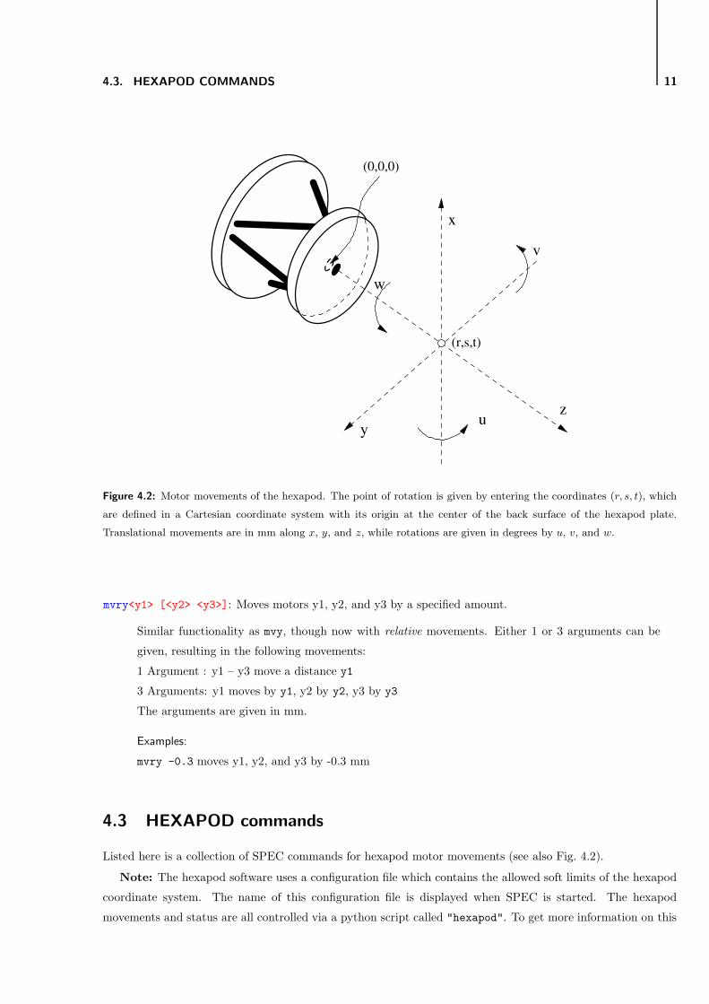
Figure 4.2: Motor movements of the hexapod. The point of rotation is given by entering the coordinates (r, s, t), which
are defined in a Cartesian coordinate system with its origin at the center of the back surface of the hexapod plate.
Translational movements are in mm along x, y, and z, while rotations are given in degrees by u, v, and w.
mvry<y1> [<y2> <y3>]: Moves motors y1, y2, and y3 by a specified amount.
Similar functionality as mvy, though now with relative movements. Either 1 or 3 arguments can be
given, resulting in the following movements:
1 Argument : y1 – y3 move a distance y1
3 Arguments: y1 moves by y1, y2 by y2, y3 by y3
The arguments are given in mm.
Examples:
mvry -0.3 moves y1, y2, and y3 by -0.3 mm
4.3 HEXAPOD commands
Listed here is a collection of SPEC commands for hexapod motor movements (see also Fig. 4.2).
Note: The hexapod software uses a configuration file which contains the allowed soft limits of the hexapod
coordinate system. The name of this configuration file is displayed when SPEC is started. The hexapod
movements and status are all controlled via a python script called "hexapod". To get more information on this
Page 16
12 MOVEMENTS, ADJUSTMENTS, AND MANIPULATIONS
script, issue the command hexapod -h in a terminal window.
Absolute scans of individual hexapod movements (u, v, w, x, y, and z) can be executed using the standard
ascan SPEC command. Axis names are uu, vv, ww, xx, yy, and zz. Note that at present, a2scan, dscan,
d2scan . . . , up to d5scan, do not work with the hexapod. Also, one cannot use SPEC to adjust the pivot point
(r, s, and t).
helpHexapod: Generates a help text similar to that given here.
This is obtained by displaying the file hexapod.txt, which should sit in the same directory as the
HEXAPOD macro file hexapod.mac.
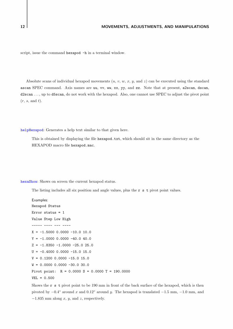
hexaShow: Shows on screen the current hexapod status.
The listing includes all six position and angle values, plus the r s t pivot point values.
Examples:
Hexapod Status
Error status = 1
Value Step Low High
----- ---- --- ----
X = -1.5000 0.0000 -10.0 10.0
Y = -1.0000 0.0000 -40.0 40.0
Z = -1.8350 -1.0000 -25.0 25.0
U = -0.4000 0.0000 -15.0 15.0
V = 0.1200 0.0000 -15.0 15.0
W = 0.0000 0.0000 -30.0 30.0
Pivot point: R = 0.0000 S = 0.0000 T = 190.0000
VEL = 0.500
Shows the r s t pivot point to be 190 mm in front of the back surface of the hexapod, which is then
pivoted by −0.4◦ around x and 0.12◦ around y. The hexapod is translated −1.5 mm, −1.0 mm, and
−1.835 mm along x, y, and z, respectively.
Page 17
4.3. HEXAPOD COMMANDS 13
hexaMove<x> <y> <z> [<u> <v> <w>]: Moves the hexapod to a specified point.
Either 3 or 6 arguments can be given, resulting in the following movements:
3 Arguments: x, y, and z move to values x, y, and z, respectively
6 Arguments: x, y, and z move to values x, y, and z, respectively (in mm) and u, v, and w move to
values u, v, and w, respectively (in degrees).
Examples:
hexaMove 0.24 -1.40 0 0.31 -0.16 0 moves x, y, and z to 0.24 mm, −1.40 mm, and 0 mm,
respectively, and rotates the hexapod plate around the x-axis by 0.31o, and around the y-axis by
−0.16o.
hmvx, hmvy, hmvz, hmvu, hmvv, hmvw<value>: Moves a hexapod axis to a specified absolute position.
The argument is given in mm for x, y, and z, and in degrees for u, v, and w.
Examples:
hmvv 0.44 rotates the hexapod plate around the y-axis by 0.44o.
hmvxr, hmvyr, hmvzr, hmvur, hmvvr, hmvwr<amount>: Relative movement of a hexapod axis by a spec-
ified amount.
The argument is given in mm for x, y, and z, and in degrees for u, v, and w.
Examples:
hmvxr 3.1 shifts the hexapod plate along the x-axis by 3.1 mm.
Page 18
14 MOVEMENTS, ADJUSTMENTS, AND MANIPULATIONS
Page 19
Chapter 5
Beam handling and security macros
This chapter deals with customized SPEC commands that enhance experimental safety and minimize radiation
damage, particularly with regards to the incident beam, beam blocking, and the direct beam falling on the
active detector area.
5.1 FAST SHUTTER commands
This set of SPEC commands deals with a fast millisecond photon shutter installed upstream of the sample, in the
direct beam. It has two main purposes – first, it will shut off the beam if SPEC sends out an error signal (e.g.,
if CTRL C is pressed). Secondly, it can be used to reduce radiation damage of the sample under investigation
by automatically closing the direct beam in between measurement points during a scan (movements can often
take as much, if not more, of the total scan time than the detector exposure time).
shutterhelp: Generates a help text similar to the listing given here.
This text is obtained by displaying on screen the file shutter.txt, which sits in the same directory
as the SHUTTER macro file shutter.mac.
shOn: Activates automatic shutter opening and closing.
The shutter is opened just before an actual count command is executed and immediately closed
again thereafter to prevent unnecessary sample irradiation.
shOff: Turns off automatic shutter opening and closing.
See shOn
shop: Opens the fast photon shutter.
Functions only if the macro shOn has been invoked.
–15–
Page 20
16 BEAM HANDLING AND SECURITY MACROS
Shutt
er
ICSlits
SR
flight tubePixel detector
fast photon shutter
Figure 5.1: The pixel detector protection system. IC = ionization chamber; SR = synchrotron radiation. The output
current from the IC will trigger the fast photon shutter to close if it is above a preset threshold.
shcl: Closes the fast photon shutter.
Functions only if the macro shOn has been invoked.
shStatus: Displays the fast photon shutter status.
Informs the user whether Automatic shutter opening is ON or Automatic shutter opening
is OFF and whether the shutter is OPEN or CLOSED. The status of the fast photon shutter is also
seen on the BEAMLINE OVERVIEW and FILTER PANEL epics widgets.
5.2 DETECTOR SHUTTER commands
A shutter is placed immediately behind a compact ionization chamber at the entrance to the detector flight
tube for protection purposes (see Fig. 5.1). The detector protection system operates as follows: if the ionization
chamber produces a current above a previously set threshold (of the order of 0.01 of that produced by the entire
direct beam), it triggers the fast photon shutter upstream of the sample to close (see Section 5.1). This does
not require that the SPEC command shOn has been invoked, as this function is hardware based). The detector
shutter at the front of the detector flight tube then closes (more slowly), filters are inserted to attenuate the
Page 21
5.3. BEAM BLOCKER COMMANDS 17
incident beam, and the fast shutter reopened. Only if the current is below the trigger threshold will the detector
shutter be reopened, and measurements can continue. Otherwise, more filters are inserted.
However, the detector shutter can also be manually opened or closed, as long as the current from the
detector-tube ionization chamber is below the threshold.
The status of the detector shutter is also seen on the BEAMLINE OVERVIEW epics widget.
pshop: Opens the shutter at the front of the detector arm.
Only works if the current from the detector ionization chamber is below its threshold value.
pshcl: Closes the shutter at the front of the detector arm.
Only works if the current from the detector ionization chamber is below its threshold value.
5.3 BEAM BLOCKER commands
The beam blocker is a tungsten rod, which can be manually positioned normal to its axis, and is translated
along its axis using the standard SPEC motor bb. The following three commands are associated with predefined
movements of bb.
bbsetup[<bbin> <bbout>]: Defines the two limit positions of the beam blocker.
BB_IN is given by bbin and should be set so that the beam is sufficiently completely occluded by the
beam blocker. BB_OUT, given by bbout, in contrast, should be so chosen that the beam blocker is
completely out of the direct beam. Values given in mm.
Examples:
bbsetup, followed by prompts for the two positions
bbsetup 10.0 4.0 sets BB_OUT to 10.0 mm and BB_IN to 4.0 mm.
bbin: Moves the beam blocker to the predefined position BB_IN.
See bbsetup.
bbout: Moves the beam blocker to the predefined position BB_OUT.
See bbsetup.
Page 22
18 BEAM HANDLING AND SECURITY MACROS
Page 23
Chapter 6
Filter and exposure settings
This chapter deals with customized SPEC commands that control beam attenuation filter positions.
There are 4 filter boxes, each containing 4 filter positions. The filter positions are labelled 1A through 4D.
15 of the 16 available filter slots are presently occupied by 5 Al (100, 200, 400, 800, and 1600 µm), 5 Ti (25, 50,
100, 200, and 400 µm), and 5 Mo (25, 50, 100, 200, and 400 µm) filters.
Macros dealing with manual filter positioning are handled in the first part of the section. In addition, a
set of commands allows the user to use automatic filtering and exposure time adjustments during experiments,
described in the second subsection.
6.1 FILTER commands
Related macros: see SHUTTER and AUTO commands.
filterhelp: Generates a help text similar to the listing given here.
This text is obtained by displaying on screen the file filter.txt, which sits in the same directory
as the FILTER macro file filter.mac.
filter<filternumber><position>: Inserts or removes filters.
The filter number (1 . . . 16) is given by filternumber. The value of position is 0 (remove) or 1
(insert).
Examples:
filter110 removes filter 11 (= 3C).
filterUp: Increases the transmission.
Using the lookup table, a subset of the filters is selected so that the transmission is increased from
its present value by the smallest possible amount.
–19–
Page 24
20 FILTER AND EXPOSURE SETTINGS
filterDown: Decreases the transmission.
Using the lookup table, a subset of the filters is selected so that the transmission is decreased from
its present value by the smallest possible amount.
filterAll: Inserts all the filters.
Often used at the start of a scan macro.
filterNone: Removes all the filters.
Use with care! This command lets through the full beam!
filterMask[<mask>]: Puts in filters specified by a mask.
The mask is a bitwise mask for all filters, 1A corresponding to the lowest bit and 4D to the highest.
The mask is given in hexadecimal notation, hence each filter box (containing 4 filters) is represented
by one character.
Examples:
filterMask prints on the screen the current filter mask.
filterMask 0x60C6 inserts filters 2 (1B), 3 (1C), 7 (2C), 8 (2D), 14 (4B), and 15 (4C), and retracts
the others.
filterGetMask(): Returns the current decimal value of the filter mask.
This is read from the EPICS channels. This macro can be used inside other macros to assign the filter
mask to a variable, e.g., mask = filterGetMask()
Examples:
If filterMask 0x0013 is sent (which puts in filters 1 (1A), 2 (1B), and 5 (2A), typing p
filterGetMask() returns 19 (= 0x0013).
filterTest: Tests if all filters are working.
All the filters are first inserted, then each one is taken out and reinserted separately. Finally, all
filters are removed again. CAUTION: Make sure no direct beam comes into any detectors while
performing this test!
Page 25
6.2. AUTO COMMANDS 21
����������������������������������������������������������������������������������������������������������
��������������������������������������
��������������������������������������
If t1, increase to t2
If t2, decrease to t1
Exposure times Filters
is greater
If t2, decrease to t1
If t2, decrease to t1 or 1s, whichever
regionRemove filters until move up out of this
Remove filters to move up toward the optimal region
Remove filters to move up toward the optimal region
No action
Insert filters to drop to the optimal region
No action
Poor
Acceptable
Good
Optimal
Saturated
TH3 = 8K
TH4 = 100K
TH1 = 40
Region counts/pixel
2t
1tTH2 = 1.5 x x TH1
Figure 6.1: Actions taken by the exposure time settings and filters for each of the five possible defined regions an image
may find itself in. Actions marked in blue take priority. If they were anyway satisfied as the image was taken, the second
piority action (if it exists) is shown in red.
6.2 AUTO commands
Related macros: see FILTER and IMAGE commands.
Macros collated under auto.mac affect the automization regarding insertion and removal of attenuation
filters and the exposure times to record data. The degree of automization is determined by autoSetLevel.mac,
described below.
The general strategy that determines the actions taken using the filters and changing exposure times is to
optimize the speed of data acquisition, even at the cost of a moderate reduction in the signal-to-noise ratio.
After each count command, the obtained counts are evaluated and compared to four threshold levels, which
define the lowest acceptable count level, the lower limit of a “good” counting range, the lower limit of the
optimal count range, and the upper limit of the optimal count range. Signal above this count rate is generally
avoided, as dead times and saturation effects must be taken into account.
Based on which region the image finds itself in, up to one action can be taken. These are summarized
graphically in Fig. 6.1.
Note: This macro is based on an earlier version by O. Bunk and R. Herger
autohelp: Generates a help text similar to the listing given here.
This text is obtained by displaying on screen the file auto.txt, which sits in the same directory as
the AUTO macro file auto.mac.
Page 26
22 FILTER AND EXPOSURE SETTINGS
autoSetLevel<autolevel>[<retries>]: Sets the automatic filter and exposure settings.
Usage: autolevel is the auto-level (i.e., the degree of automation) and can take on three values:
0 – automatic filter and exposure OFF
1 – automatic filter ON, automatic exposure changes OFF
2 – automatic filter and exposure changes ON
retries optionally specifies the maximum number of retries before giving up (default value = 20).
Examples:
autoSetLevel 2 15 sets both automatic filter and exposure ON and allows a maximum number of 15
attempts to optimize. The automatic change in exposure times is set by autoSetExposure.
autoSetExposure<lowerexptime><upperexptime>: Sets the automated exposure times.
This command is needed if autoSetLevel is set to 2 (i.e., automatic filter and exposure ON, see
above).
Usage: lowerexptime sets the shorter and upperexptime the longer exposure times in seconds.
Examples:
autoSetExposure 1 10 sets the shorter exposure time to 1 s, the longer to 10 s.
autoShow: Shows the current autoSetLevel settings.
Returns on the screen the autoSetLevel value (0, 1, or 2) and the shorter and longer exposure times.
Page 27
Chapter 7
Area detector macros
This chapter deals with customized SPEC commands used for setting up, formatting and controlling 2-dimensional
area detectors, in particular the Pilatus photon-counting pixel detector.
7.1 PIXEL commands
The pixel detector is a PSI-developed instrument. The first model, Pilatus I, has an array of 366 x 157 pixels.
A newer model, Pilatus II, has an array of 487 x 195 pixels.
pixhelp: Generates a help text similar to the listing given here.
This text is obtained by displaying on screen the file pixel.txt, which sits in the same directory
as the PIXEL macro file pixel.mac.
pixon: Turns on the pixel detector.
Also automatically turns of any other detector connected to the system.
pixoff: Turns off the pixel detector.
Also automatically turns on the point detector.
pixconnected(): Checks whether pixel detector is properly connected with SPEC via EPICS.
Returns 1 if the pixel is connected, 0 otherwise.
pixsetup: Sets up the pixel detector.
The user is prompted with several questions.
–23–
Page 28
24 AREA DETECTOR MACROS
pixsetpath: Specifies the path for pixel detector image files.
The user is prompted to give a path to the desired image directory. pixsetpath is a subcommand
of pixsetup.
pixsetfmt: Specifies the name template for image files.
The user is prompted to give a filename template format. pixsetfmt is a subcommand of pixsetup.
pixsetexpose<pixexptime>: Sets the pixel exposure time.
Given in seconds. pixsetexpose is a subcommand of pixsetup.
Examples:
pixsetexpose 5 sets the pixel exposure time to 5 s.
pixshow: Shows the detailed current pixel detector settings.
An example of the screen output:
The PILATUS pixel detector is currently enabled.
To disable it type ’pixoff’.
The current pixel detector settings are:
The frame number = 9999
The file path is: temp/
The file template is: image_%05d.img
The last file name was: image_10173.img
The next file name will be: image_10000.img
Exposure time = 1.000 sec
Image dimensions: 366 x 157 pixels (total = 57462)
Threshold values: Thresh1 = 40, Thresh2 = 400, Thresh3 = 8000
Image analysis is currently enabled.
The active imaging device name is: PILATUS
signal region of interest : (105, 75) (125, 95)
background region of interest: ( 95, 65) (135,105)
image dimensions (x*y) : 366 * 157 pixels
Page 29
7.1. PIXEL COMMANDS 25
pixsnap[<filename>]: Tells the pixel detector to take an image and write it to disk.
If the optional argument filename is given, it will be used to specify the file which is to be written.
This filename is assumed to be relative to the filename path defined by pixsetpath.
If no argument is given, the frame number will be incremented and a filename will be generated
from the filename template.
pixUndo: Decrements the pixel detector image number by 1
Used before repeating the exposure and overwriting the last file.
pixresnap: Tells the pixel detector to take an image and overwrite the previous disk file.
Incorporates the command pixUndo
pixwait: Waits for the pixel detector to become ”Ready”.
Used after pixsnap or pixresnap.
pixsw[<filename>]: Calls pixsnap and then pixwait.
filename is the optional filename argument.
pixlogon[<arg1>]: Turns on logging of EPICS stuff for each pixel snap.
The optional argument arg1 specifies the directory for the log files. If this is not given, the user
will be prompted.
pixlogoff: Turns off logging of EPICS stuff for each pixel snap.
See also pixlogon.
pixlogshow: Displays the current snap logging status.
Either ON or OFF.
pixlogwrite[<filename>]: Writes a pixel detector snap log file.
Writes a PIXEL snap log file. The file name is either derived from the name of the image file or is
given by the optional argument filename.
Page 30
26 AREA DETECTOR MACROS
7.2 CCD commands
Presently, no detector based on charge-coupled device (CCD) technology is implemented in SPEC at the SD
station of the MS beamline. As and when this changes, commands will be added. The functionalty should be
such that they should be compatible with the IMAGE commands described below.
7.3 IMAGE commands
In this section, macros are described which are used to analyze images (taken by any sort of imaging device)
on-line during data acquisition and return a set of characteristic values to SPEC. It is thus possible to plot
results of a scan (usually an intensity value) during data acquisition using the imaging device, just like one
would with a point detector. Furthermore, the image information can be used to automate filter transmission
and exposure time settings during a scan (refer to auto.mac for more information on automated scans).
imagehelp: Generates a help text similar to the listing given here.
This text is obtained by displaying on screen the file image.txt, which sits in the same directory
as the IMAGE macro file image.mac.
imageInit: Initializes all global variables used by image.mac.
Used as part of starting up the imaging algorithms.
imageOn: Turns on image analysis.
Turns on the macro functionality to analyze images acquired by an area detector on-line and return
the results to SPEC. imageOn is usually called at startup (in sdStartup) and in enabling macros
of 2D-detectors, such as in pixon.
imageOff: Turns off image analysis.
Turns off the macro functionality to analyze images acquired by an area detector.
imageShow: Shows whether image analysis is currently enabled or disabled.
Also displays the region of interest (ROI) settings (see below).
Page 31
7.3. IMAGE COMMANDS 27
y
x(0,0)
(486,194)
(SX1,SY1)
(BX1,BY1)
(SX2,SY2)
(BX2,BY2)
Figure 7.1: Definition of the regions of interest (ROIs). The white frame encompasses the feature to be analyzed and is
defined by the x- and y-coordinates of the upper left hand corner (arg1,arg2) and those of the lower right hand corner
(arg3,arg4). Similarly, a background box (in red) is defined by (arg5,arg6) and (arg7,arg8). An alternative background
ROI is given by the dashed red frame.
imageSetRoi[<SX1> <SY1> <SX2> <SY2> <BX1> <BY1> <BX2> <BY2>]: Sets the regions of interest (ROIs)
for intensity and background integration.
See Fig. 7.1. By only supplying 4 arguments (<SX1> - <SY2>), or by setting the coordinates of the
background box identically equal to those of the signal box, no background subtraction is performed.
Examples:
imageSetRoi 105 50 200 100 95 40 210 105 sets a signal ROI with its top left corner at pixel
(105,50) and bottom right corner at (200,100). The background ROI roduces a border region 10
pixels wide around the signal ROI.
imageSetRoi shows the currently defined ROIs.
imageCheckRoi: Checks the regions of interest for consistency with the the image dimensions, etc.
Requires a knowledge of the image size. See e.g., pixsetup.
imageGetInt: This macro analyzes the last image taken by the active area detector.
Checks the ROIs defined by imageSetRoi and sets some global variables to the intensity values
determined. Calling parameters are the three threshold values. The number of pixels with intensity
above these values is returned.
Page 32
28 AREA DETECTOR MACROS
Page 33
Chapter 8
Reciprocal space commands
In this chapter, we list the customized SPEC commands for navigating in reciprocal space. In order to give a
complete overview of the facilities available in reciprocal space movements, some “standard” reciprocal space
functions are also described.
8.1 Preparatory commands
In general, reciprocal space movements require some pre-knowledge about several aspects of the experimental
setup, including energy/wavelength settings, sample parameters (lattice parameters, critical angles for total
external reflection, etc.),
defenergy<energy>: Defines the wavelength using the energy of the x-radiation being used.
This command is used for those users who prefer to think in keV than Angstrom. By setting the
energy (given in keV), this macro calculates the wavelength in Angstrom, which is then used to in-
ternally call up setlambda . The conversion is given by
λ[A] =12.39828
E[keV].
Examples:
defenergy 16 sets the x-ray energy to 16 keV and informs SPEC via setlambda that the wavelength
is 0.77489 A.
–29–
Page 34
30 RECIPROCAL SPACE COMMANDS
setlambda<lambda> : Sets the wavelength of the x-radiation being used.
Sets the wavelength of the x-radiation being used in A. This is needed in order to perform reciprocal
space calculations.
Examples:
setlambda 1 sets the wavelength to 1 A, which corresponds to an x-ray wavelength of 12.398 keV.
setlat[<a> <b> <c> <alpha> <beta> <gamma>] : Sets the 6 crystal lattice parameters.
Standard SPEC macro command. Sets the 6 crystal lattice parameters, a, b, and c in A, and α, β,
and γ in degrees. Often, it is convenient to redefine the crystal lattice from its bulk values to so-called
surface coordinates, for which c (and therefore l) are perpendicular to the sample surface (ignoring
any small miscut angles). This is discussed in detail in the angle calculations manual.
By typing in setlat alone, the user is prompted to give the six lattice parameters one by one.
Examples:
setlat 7.723 7.707 7.723 90 89.2656 90 was used for setting up the surface coordinate system
for a NdGaO3(110) surface, whose bulk lattice parameters are a = 5.426 A, b = 5.496 A, c = 7.707 A,
α = β = γ = 90o.
setcritang<critang> : Sets the critical angle for total external reflection.
This macro is used to obtain the critical angle, which is then used by the macro setrestrict.
Examples:
setcritang 0.17 sets the critical angle to 0.17o.
setrestrict<state>: Turns on or off consideration of refraction effects
Turns on (1) or off (0) the functionality to include refraction effects in determining the positions
of x-ray reflections. The critical angle for total external reflection is required. Presently, this
functionality is not implemented.
Page 35
8.1. PREPARATORY COMMANDS 31
setmode[<mode>]: Sets the recording mode of reciprocal space scans.
Standard SPEC macro command. Sets the recording mode of reciprocal space scans. Three modes
are possible:
0 = fixed incident beam angle (betain)
1 = fixed exit beam angle (betaout)
2 = incident angle equal to exit angle (betain = betaout)
By typing in setmode alone, the user is prompted to enter the desired mode (0, 1, or 2).
Examples:
setmode 0 sets the diffractometer to fixed incident angle scans.
freeze[<beta>]: Freezes the incident or exit angle.
Standard SPEC macro command. Freezes the incident angle betain to beta if setmode = 0, or the
exit angle betaout to beta if setmode = 1. Will return an error if used in setmode 2. If no parameter
is typed in, the present incident angle (for setmode = 0) or exit angle (for setmode = 1) will be
adopted.
Examples:
freeze 0.15 sets either betain or betaout to 0.15o, depending on the diffractometer mode.
setnurot<numode>: Sets the nu-rotation mode.
Sets the nu-rotation mode to one of three possibilities.
0 – no nu-rotation
1 – rotation of nu so that the projection of the perpendicular component of the momentum transfer l
remains parallel to the detector slits
2 – rotation of nu so that the projection of the x-ray footprint on the sample remains parallel to the
detector slits
If no argument is entered, the user is prompted to enter values 0, 1, or 2.
Examples:
setnurot 2 sets nu rotation to the “static footprint” mode.
Page 36
32 RECIPROCAL SPACE COMMANDS
8.2 Orientation matrix commands
Many of the below customized commands are extended wrap-arounds for standard SPEC commands, developed
to provide a more powerful and intuitive user interface.
orientHelp : Generates a help text similar to the listing given here.
This text is obtained by displaying on screen the file orient.tex, which sits in the same directory
as the ORIENT macro file orient.tex.
orientMiscut[<rho> <sigma> <tau>]: Sets the three miscut angles ρ, σ and τ .
Sets the three miscut angles ρ, σ and τ used to account for miscuts of crystal surfaces, i.e., the difference
between the physical surface and the crystal planes associated with the crystals nominal orientation.
These angles can also in principle be used to describe one crystal orientation using coordinates of
another crystal orientation. So, for example, a cubic (111) surface with its (1-10) axis along the x-axis
can be described as being a cubic (001) surface with miscut angles ρ = −45o, σ = −35.2644o, and
τ = −60o. This realignment is discouraged, however, as it means that scans recorded perpendicular
to the surface are not described by changes in the l-coordinate. Instead, the adoption of a unit cell
described by surface coordinates is recommended.
By typing in setmiscut alone (no arguments), the user is prompted to enter the miscut angles
individually.
Examples:
setMiscut 0.014 -0.028 89.710 manually sets the miscut of a sample to ρ = 0.14o, σ = −0.028o,
and τ = 89.710o.
orientClear : Clears the list of measured reflections.
Should be called before one starts to obtain reflections for the orientation matrix.
showUB : Shows the UB matrix.
A typical output might look something like this:
100.X04V> showUB
Orientation matrix by row
Row 1: -0.01352 -0.81339 -0.00993
Row 2: 0.81527 -0.01351 -0.00013
Row 3: 0.00005 0.00064 0.81429
Page 37
8.2. ORIENTATION MATRIX COMMANDS 33
orientAdd<h> <k> <l> [<pos1> <pos2> ...<posn>]: Adds the reflection (h k l) to the list of measured
reflections.
Usage: <h>, <k>, and <l> must be integers. If only the parameters <h>, <k>, and <l> are entered, the
current diffractometer angles are used. If the diffractometer angles are defined by the user, <pos1>
<pos2> ...<posn> are the diffractometer motor positions in the same order as they appear in the
configuration file (use wh). A check is made that the reflection does not already exist in the reflection
file.
Examples:
orientAdd 1 0 2 adds the (1 0 2) reflection to the reflection file.
orientRemove<h> <k> <l>: Removes the reflection (h k l) from the list of measured reflections.
After checking that it is already in the list of measured reflections, the specified reflection is removed
from that list.
Examples:
orientRemove 1 0 2 removes the (1 0 2) reflection from the reflection file.
orientReplace<h> <k> <l> [<pos1> <pos2> ...<posn>]: Replaces the motor positions for the reflection
(h k l) in the list of measured reflections, either with the current motor positions, or with user-defined
motor positions.
Usage: <h>, <k>, and <l> must be integers. If only the parameters <h>, <k>, and <l> are entered, the
current diffractometer angles are used. If the diffractometer angles are defined by the user, <pos1>
<pos2> ...<posn> are the diffractometer motor positions in the same order as they appear in the
configuration file (use wh). A check is made that the reflection already exists in the reflection file.
Examples:
orientReplace 1 0 2 replaces the diffractometer motor positions already in the list-of-reflections file
for the (1 0 2) reflection with the values for the current motor positions.
Page 38
34 RECIPROCAL SPACE COMMANDS
orientFit : Performs an orientation matrix fit.
This function determines the miscut (or “Euler”) angles of the crystal under investigation and
also returns a goodness of fit (values for this below ≈ 10−2 are acceptable). The fitting procedure
requires the angular coordinates of at least three reflections with known hkl indices, entered using
orientAdd. Acceptance of the newly calculated miscut angles must be actively given (by typing y
or yes) by the user. A typical output looks similar to this:
101.X04V> orientFit
Reflections file (Reflex)?
# Sat Sep 23 01:22:24 2006
_fitUB
(Using fitted UB.)
Goodness of fit = 2.877910e-05
Old miscut angles: 0.00115, -0.0233, -0.0991
New miscut angles: -90.9514, -0.0451, -0.0037
Use these angles? (NO)? y
Page 39
8.2. ORIENTATION MATRIX COMMANDS 35
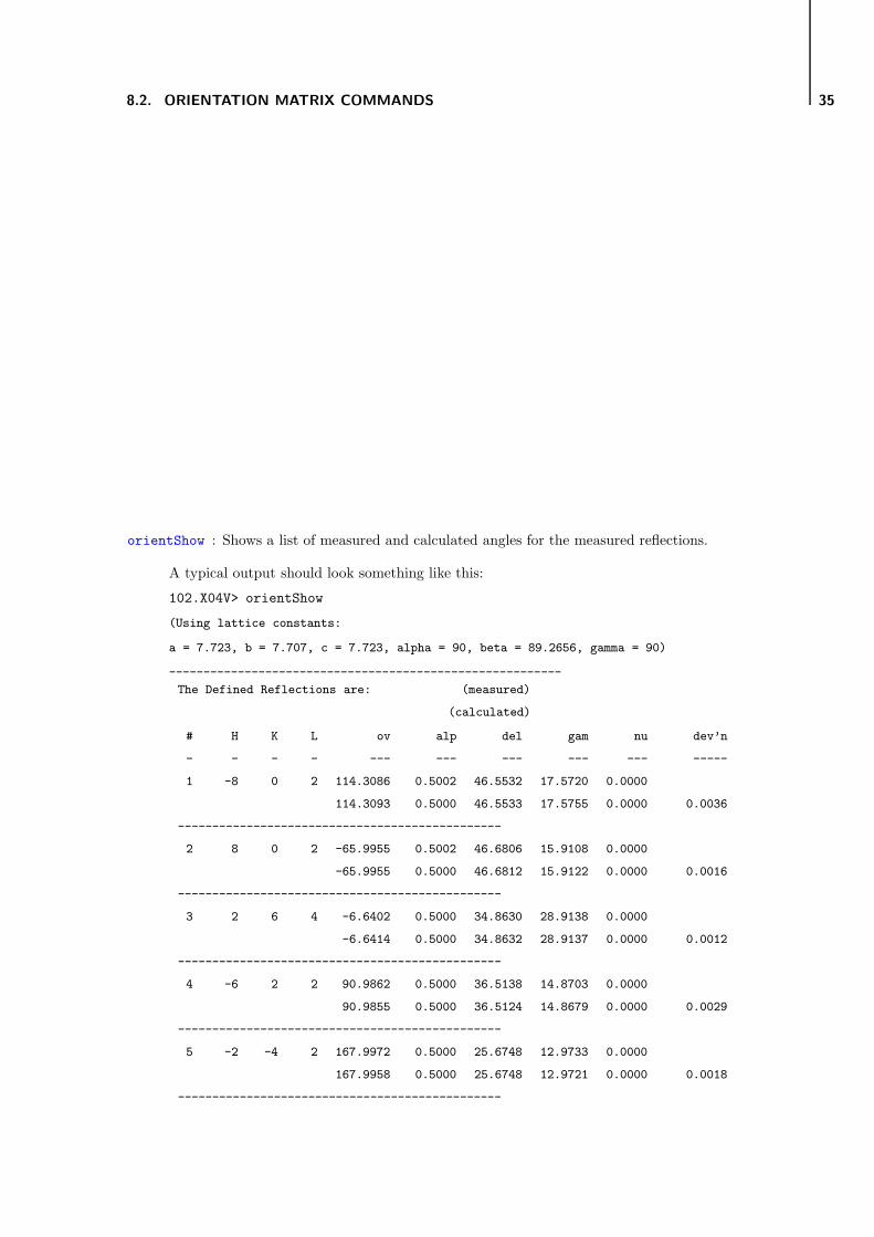
orientShow : Shows a list of measured and calculated angles for the measured reflections.
A typical output should look something like this:
102.X04V> orientShow
(Using lattice constants:
a = 7.723, b = 7.707, c = 7.723, alpha = 90, beta = 89.2656, gamma = 90)
---------------------------------------------------------
The Defined Reflections are: (measured)
(calculated)
# H K L ov alp del gam nu dev’n
- - - - --- --- --- --- --- -----
1 -8 0 2 114.3086 0.5002 46.5532 17.5720 0.0000
114.3093 0.5000 46.5533 17.5755 0.0000 0.0036
-----------------------------------------------
2 8 0 2 -65.9955 0.5002 46.6806 15.9108 0.0000
-65.9955 0.5000 46.6812 15.9122 0.0000 0.0016
-----------------------------------------------
3 2 6 4 -6.6402 0.5000 34.8630 28.9138 0.0000
-6.6414 0.5000 34.8632 28.9137 0.0000 0.0012
-----------------------------------------------
4 -6 2 2 90.9862 0.5000 36.5138 14.8703 0.0000
90.9855 0.5000 36.5124 14.8679 0.0000 0.0029
-----------------------------------------------
5 -2 -4 2 167.9972 0.5000 25.6748 12.9733 0.0000
167.9958 0.5000 25.6748 12.9721 0.0000 0.0018
-----------------------------------------------
Page 40
36 RECIPROCAL SPACE COMMANDS
8.3 Move and scan commands
These commands allow one to move to positions and navigate linearly in reciprocal space.
mvhkl<h> <k> <l> [auto]: Moves to a point hkl in reciprocal space.
This is a wrap-around for the standard SPEC macro br. If the optional auto is not included, the
calculated angles are shown and the user is asked if he/she really wants to move there:
104.X04V> mvhkl 2 0 2
OmegaV = -8.3935 --> -80.0090
Alpha = 0.5000 --> 0.5000
Delta = 25.9640 --> 11.3530
Gamma = 33.5000 --> 11.6550
Nu = 0.0000 --> 0.0000
Move to these values? (YES)?
If the movement is physical impossible, an error message will be appear. By typing -auto after the
l-value (and not forgetting a space in between), the movement will be executed immediately, without
the user prompt.
Examples:
mvhkl 1 2 1 auto moves the diffractometer angles to the nominal position in reciprocal space 1 2 1
without prompting the user to confirm the movement.
br, ubr, mk, umk<h> <k> <l>: Commands to move to points in reciprocal space.
Standard SPEC macros. The mk macro is used to move the diffractometer to the reciprocal space
point (hkl). The umk macro also moves the diffractometer, but provides an updated display of the
motor positions and corresponding reciprocal space coordinates while the motors are moving. The
update interval, in seconds, is set by the global variable UPDATE.
mk is synonymous with br, umk with ubr.
Examples:
umk -1 1 2 moves the diffractometer to the reciprocal space point (−112), while updating the progress
on-screen during the movement.
Page 41
8.3. MOVE AND SCAN COMMANDS 37
hklscan<hstart> <hend> <kstart> <kend> <lstart> <lend> <intervals> <time>: Performs a linear
scan between two points in reciprocal space.
Standard SPEC macro. It performs a linear scan in reciprocal space over the three coordinates hkl
which range from hstart, kstart, and lstart to hend, kend, and lend, respectively. The step size
for each coordinate is (start - end)/intervals. The number of data points collected is intervals + 1.
The count time is given by time, which if positive, specifies the exposure in seconds, and, if negative,
specifies monitor counts.
Examples:
hklscan 0.4 2.4 0.4 2.4 0.1 0.1 50 2 instructs the diffractometer to perform a near in-plane
scan (l = 0.1) across a diagonal in hk-space between h = k = 0.4 and h = k = 2.4 in 50 steps (step
size 0.04 r.l.u.), taking a 2 second exposure at each point.
hscan, kscan, lscan<start> <end> <intervals> <time>: A linear scan in one of the reciprocal coordi-
nates h, k, or l.
Standard SPEC macro. A linear scan in reciprocal space along the one of the principal reciprocal
axes from start to end. The step size is (start - end)/intervals. The number of data points
collected will be intervals + 1. Count time is given by time, which, if positive, specifies seconds
and, if negative, specifies monitor counts. Note that the other two reciprocal coordinates have not
been specified, that is, if hscan is called, this will be performed in the plane defined by the present
values of k and l.
Examples:
kscan 0.0 4.0 40 1 instructs the diffractometer to perform a scan from k = 0.0 to 4.0 in steps of
0.1 and exposure times of 1 s.
Page 42
38 RECIPROCAL SPACE COMMANDS
hkcircle klcircle hlcircle<radius> <stang> <endang> <intervals> <time> [<exprn>]: A circular
(arc) scan in the plane of two of the reciprocal coordinates h, k, or l.
Standard SPEC macro. A circular arc scan in reciprocal space in the plane of two of the prin-
cipal reciprocal axes of radius radius (in r.l.u.) from stang to endang. The step size is (stang -
endang)/intervals. The number of data points collected will be intervals + 1. Count time is given
by time, which, if positive, specifies seconds and, if negative, specifies monitor counts. Note that the
other reciprocal coordinate is not specified, that is, if hkcircle is called, this will be performed in
the plane defined by the present value of l. The optional argument exprn defines an expression to be
evaluated after h and k have been calculated at each scan point.
Examples:
hkcircle 3.0 0 90 45 1 ’’L = H/14 + 0.1’’ instructs the diffractometer to perform an arc scan
from 0o to 90o, with a radius of 3.0 r.l.u. and at l-values of h/14 + 0.1 in steps of 2 degr and exposure
times of 1 s.
twh, twk, twl : Not yet functional.
Not yet functional.
Examples:
To be defined.
8.4 Calculation commands
ca<h> <k> <l>: Prints calculated motor settings for the reciprocal space position (hkl).
The ca macro prints out the calculated motor settings for the reciprocal space position given by the
arguments h, k, and l. After printing the motor information, the values in the A[] array (the array
dimensioned to the number of motors, as obtained from the config file) and the values of the reciprocal
space coordinates are restored to the current diffractometer position.
Examples:
ca 1 1 3 will give the relevant diffractometer motor positions to move to the reciprocal space point
(113).
Page 43
8.4. CALCULATION COMMANDS 39
ci<mot1> <mot2> <mot3> <mot4>: Display calculated h, k, and l values for input angles.
Standard SPEC macro. The arguments mot1, mot2, mot3, and mot4 are defined in the same order as
they appear in the config file and in the case of vertical geometry (X04V) are omegav, alpha, delta,
and gamma, while for the horizontal geometry (X04H), they are phi, omegah, delta, and gamma.
Examples:
ci 10 0.5 25 40 in X04V will return the values of h, k, and l for ov = 10, alp = 0.5, delta = 25,
and gamma = 40.
wh : Displays reciprocal space positions and motor positions.
Standard SPEC macro. Displays a list of positions in reciprocal and real space.
Page 44
40 RECIPROCAL SPACE COMMANDS
Page 45
Chapter 9
Sundry commands
9.1 Plotting commands
The plotting commands described in this section help in producing the best on-screen and printing outputs
pplot : Prints out SPEC-supported scans.
Standard SPEC macro.
–41–
Page 46
42 SUNDRY COMMANDS
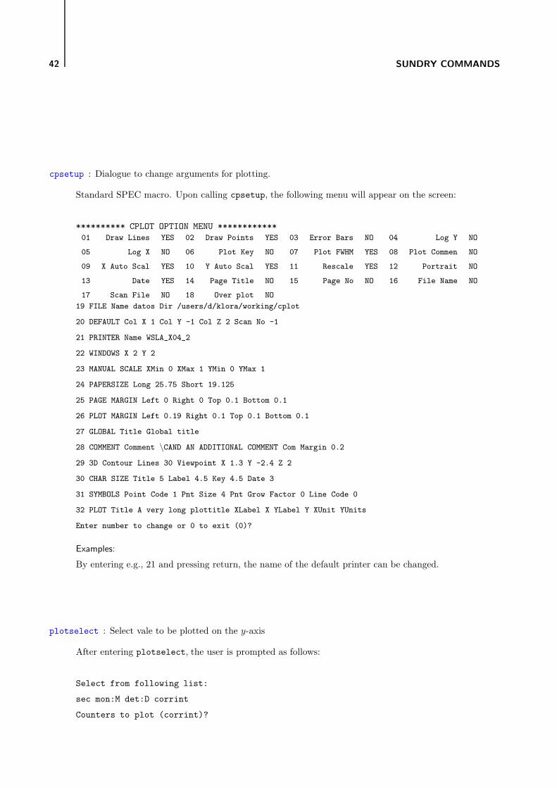
cpsetup : Dialogue to change arguments for plotting.
Standard SPEC macro. Upon calling cpsetup, the following menu will appear on the screen:
********** CPLOT OPTION MENU ************
01 Draw Lines YES 02 Draw Points YES 03 Error Bars NO 04 Log Y NO
05 Log X NO 06 Plot Key NO 07 Plot FWHM YES 08 Plot Commen NO
09 X Auto Scal YES 10 Y Auto Scal YES 11 Rescale YES 12 Portrait NO
13 Date YES 14 Page Title NO 15 Page No NO 16 File Name NO
17 Scan File NO 18 Over plot NO
19 FILE Name datos Dir /users/d/klora/working/cplot
20 DEFAULT Col X 1 Col Y -1 Col Z 2 Scan No -1
21 PRINTER Name WSLA_X04_2
22 WINDOWS X 2 Y 2
23 MANUAL SCALE XMin 0 XMax 1 YMin 0 YMax 1
24 PAPERSIZE Long 25.75 Short 19.125
25 PAGE MARGIN Left 0 Right 0 Top 0.1 Bottom 0.1
26 PLOT MARGIN Left 0.19 Right 0.1 Top 0.1 Bottom 0.1
27 GLOBAL Title Global title
28 COMMENT Comment \CAND AN ADDITIONAL COMMENT Com Margin 0.2
29 3D Contour Lines 30 Viewpoint X 1.3 Y -2.4 Z 2
30 CHAR SIZE Title 5 Label 4.5 Key 4.5 Date 3
31 SYMBOLS Point Code 1 Pnt Size 4 Pnt Grow Factor 0 Line Code 0
32 PLOT Title A very long plottitle XLabel X YLabel Y XUnit YUnits
Enter number to change or 0 to exit (0)?
Examples:
By entering e.g., 21 and pressing return, the name of the default printer can be changed.
plotselect : Select vale to be plotted on the y-axis
After entering plotselect, the user is prompted as follows:
Select from following list:
sec mon:M det:D corrint
Counters to plot (corrint)?
Page 47
9.2. SMS COMMANDS 43
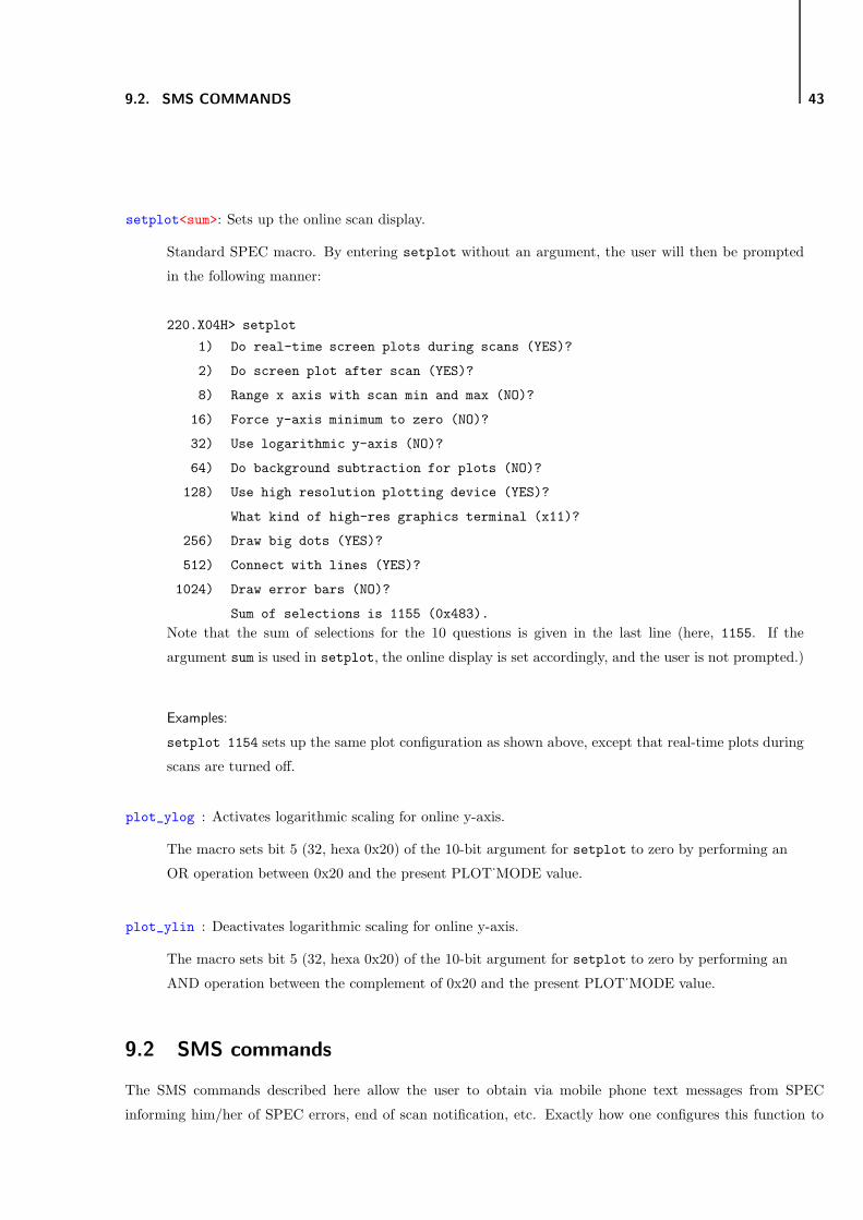
setplot<sum>: Sets up the online scan display.
Standard SPEC macro. By entering setplot without an argument, the user will then be prompted
in the following manner:
220.X04H> setplot
1) Do real-time screen plots during scans (YES)?
2) Do screen plot after scan (YES)?
8) Range x axis with scan min and max (NO)?
16) Force y-axis minimum to zero (NO)?
32) Use logarithmic y-axis (NO)?
64) Do background subtraction for plots (NO)?
128) Use high resolution plotting device (YES)?
What kind of high-res graphics terminal (x11)?
256) Draw big dots (YES)?
512) Connect with lines (YES)?
1024) Draw error bars (NO)?
Sum of selections is 1155 (0x483).
Note that the sum of selections for the 10 questions is given in the last line (here, 1155. If the
argument sum is used in setplot, the online display is set accordingly, and the user is not prompted.)
Examples:
setplot 1154 sets up the same plot configuration as shown above, except that real-time plots during
scans are turned off.
plot_ylog : Activates logarithmic scaling for online y-axis.
The macro sets bit 5 (32, hexa 0x20) of the 10-bit argument for setplot to zero by performing an
OR operation between 0x20 and the present PLOT˙MODE value.
plot_ylin : Deactivates logarithmic scaling for online y-axis.
The macro sets bit 5 (32, hexa 0x20) of the 10-bit argument for setplot to zero by performing an
AND operation between the complement of 0x20 and the present PLOT˙MODE value.
9.2 SMS commands
The SMS commands described here allow the user to obtain via mobile phone text messages from SPEC
informing him/her of SPEC errors, end of scan notification, etc. Exactly how one configures this function to
Page 48
44 SUNDRY COMMANDS
include a given mobile number is given interactively in smsSetup.
smshelp : Generates a help text similar to the listing given here.
This text is obtained by displaying on screen the file sms.txt, which sits in the same directory as
the SMS macro file sms.mac.
smsSetup : Sets up the sms header information
Defines information including: sender, recipients, etc. The user is prompted interactively to follow
the instructions.
smsOn[auto]: Enables the SMS notification service.
The user is prompted whether SPEC errors should also be reported. If the optional ”auto” argument is
used, this prompt is circumvented and errors are automatically reported (for use inside other macros).
This requires that smsSetup has already been executed.
Examples:
smsOn – user has to confirm he really wants this functionality.
smsOn auto – sms notification service is enabled and SPEC errors are reported.
smsOff: Turns off the sms notification service.
It is strongly recommended to include this macro at the end of a long-scan macro, in order to avoid
being bombarded with SMS error messages, etc. – for example, every time CNTL-C is pressed to
stop a short scan, halt a motor movement, etc., SPEC will send an error message if smsOff has not
been implemented.
smsSendScanSuccess: Sends the predefined success message ”SPEC-scan completed successfully”.
Often added at the end of a long-scan macro, so the user doesn’t have to keep checking how the
scan is progressing.
smsSendError: Sends the predefined error message ”SPEC - Error encountered; scan aborted”.
One can include this in a macro, for example in an IF statement, to inform the user that some
check in the macro has detected an error. This is also added internally to the cleanup_once macro
of SPEC, used if SPEC crashes.
Page 49
9.2. SMS COMMANDS 45
smsSendMessage(‘‘<message_string>’’): Sends a user-defined message.
This macro function sends a user-defined message, passed as a string variable argument.
Examples:
smsSendMessage("SPEC error -- scan aborted")
Page 50
46 SUNDRY COMMANDS
Page 51
Index
autoSetExposure , 22
autoSetLevel , 22
autoShow , 22
autohelp , 21
bbin , 17
bbout , 17
bbsetup , 17
br, ubr, mk, umk , 36
ca , 38
ci , 39
cpsetup , 42
defenergy , 29
filter , 19
filterAll , 20
filterDown , 20
filterGetMask() , 20
filterMask , 20
filterNone , 20
filterTest , 20
filterUp , 19
filterhelp , 19
freeze , 31
helpHexapod , 12
hexaMove , 13
hexaShow , 12
hkcircle klcircle hlcircle , 38
hklscan , 37
hmvx, hmvy, hmvz, hmvu, hmvv, hmvw , 13
hmvxr, hmvyr, hmvzr, hmvur, hmvvr, hmvwr , 13
hscan, kscan, lscan , 37
imageCheckRoi , 27
imageGetInt , 27
imageInit , 26
imageOff , 26
imageOn , 26
imageSetRoi , 27
imageShow , 26
imagehelp , 26
movehelp , 9
mvhkl , 36
mvry , 11
mvy , 10
orientAdd , 33
orientClear , 32
orientFit , 34
orientHelp , 32
orientMiscut , 32
orientRemove , 33
orientReplace , 33
orientShow , 35
pixUndo , 25
pixconnected() , 23
pixhelp , 23
pixlogoff , 25
pixlogon , 25
pixlogshow , 25
pixlogwrite , 25
pixoff , 23
pixon , 23
pixresnap , 25
pixsetexpose , 24
pixsetfmt , 24
pixsetpath , 24
pixsetup , 23
pixshow , 24
pixsnap , 25
pixsw , 25
pixwait , 25
plot_ylin , 43
plot_ylog , 43
–47–
Page 52
48 INDEX
plotselect , 42
pplot , 41
pshcl , 17
pshop , 17
sdStartup , 4
sdhelp , 4
setcritang , 30
setlambda , 30
setlat , 30
setmode , 31
setnurot , 31
setplot , 43
setrestrict , 30
shOff , 15
shOn , 15
shStatus , 16
shcl , 16
shop , 15
showUB , 32
shutterhelp , 15
smsOff , 44
smsOn , 44
smsSendError , 44
smsSendMessage , 44
smsSendScanSuccess , 44
smsSetup , 44
smshelp , 44
twh, twk, twl , 38
wh , 39