97
Guide to Designing Geocellular Drainage Systems to CIRIA Report C737 September 2018

Guide to Designing Geocellular Drainage
Systems to CIRIA Report C737
September 2018

Page 2 © BPF Pipes Group, 2018
Contents
Contents ................................................................................................................................................................... 2
1. Introduction .................................................................................................................................... 5
2. Design process ................................................................................................................................ 6
2.1 Process ........................................................................................................................................................ 6
2.2 Accidental loading ..................................................................................................................................... 8
2.3 Temporary construction situation ........................................................................................................ 8
3. Details for the worked example in this guide ................................................................................. 9
4. Layout of the worked example in this guide ................................................................................. 11
5. Preliminaries ................................................................................................................................. 12
5.1 Project Roles and Sign Off Sheet ........................................................................................................ 12
5.2 Designer Evaluation Form ..................................................................................................................... 14
6. Step 1: Determine site classification, design class and design/checking requirements ............... 16
6.1 Worked example .................................................................................................................................... 16
6.2 Results of the site classification and implications ............................................................................ 20
6.3 Generic classification system for routine sites ................................................................................ 20
7. Step 2: Develop the conceptual ground model ............................................................................ 22
8. Step 3: Determine characteristic loads and apply partial factors to give design loads ................ 24
8.1 Loads .......................................................................................................................................................... 24
8.2 Step 3.1: Vertical characteristic load from backfill and surcharge ............................................... 24
8.2 Step 3.2: Vertical characteristic traffic loading ................................................................................. 26
8.3 Step 3.3: Lateral characteristic load from earth pressure and groundwater ............................ 32
8.4 Step 3.4: Lateral characteristic load from wheel loads adjacent to tank ................................... 34
8.5 Step 3.5: Partial factors of safety for loads and soil properties ................................................... 40
8.6 Step 3.6: Design vertical loads ............................................................................................................. 42
8.7 Step 3.7: Design lateral loads ............................................................................................................... 44
9. Step 4: Determine characteristic strength and apply partial factors to determine design
properties .............................................................................................................................................. 46
9.1 Strength data ............................................................................................................................................ 46
9.2 Step 4.1: Partial material factors of safety ......................................................................................... 46
9.3 Step 4.2: Design strengths .................................................................................................................... 50
9.4 Step 4.3: Product Evaluation Form ..................................................................................................... 52

Page 3 © BPF Pipes Group, 2018
9.5 Step 4.4: Additional data to be appended to Product Evaluation Form .................................... 54
10. Step 5: Design calculations and analysis ................................................................................... 56
10.1 Step 5.1: Compare design load to design strength ......................................................................... 56
10.2 Step 5.2: Compare predicted tank deformation to acceptable limits for the site ................... 59
10.3 Step 5a: Global deformation and site stability assessment............................................................ 66
11. Step 6: Prepare geotechnical design report ............................................................................. 67
12. Additional information .............................................................................................................. 70
12.1 Existing tanks ............................................................................................................................................ 70
12.2 Testing ....................................................................................................................................................... 70
Appendix A: Summary of key features of C680, C737 and the BPF Pipes Group guide to C737 .......... 72
Appendix B: Traffic zones and site classification .................................................................................. 74
Traffic Zones ......................................................................................................................................................... 74
Examples of traffic zones .................................................................................................................................... 75
Site classification for the traffic zones ............................................................................................................. 77
Appendix C: Wheel and surcharge loads plus factors to be used to calculate characteristic traffic
loads ...................................................................................................................................................... 79
Loads ..................................................................................................................................................................... 79
Load factors ........................................................................................................................................................... 80
Appendix D: Braking forces ................................................................................................................... 82
Appendix E: Lateral loads and arching .................................................................................................. 84
Introduction ........................................................................................................................................................... 84
Evidence for arching effects ............................................................................................................................... 84
Design parameters ............................................................................................................................................... 86
Summary of the finite element analysis ........................................................................................................... 86
Ground truthing the model ............................................................................................................................... 92
Conclusions ........................................................................................................................................................... 92
Appendix F: Overall design approach ................................................................................................... 95
Appendix G: Determining yield strength from short-term tests – the BBA approach ......................... 97

Page 4 © BPF Pipes Group, 2018
It has been assumed in the drafting of this guidance that the execution of its provisions is entrusted
to appropriately qualified and experienced people. Compliance with this guide does not itself confer
immunity from legal obligations and all relevant National Legislation and Standards apply.
Information contained in this guidance is given in good faith. The British Plastics Federation (BPF)
Pipes Group cannot accept any responsibility for actions taken by others as a result.

Page 5 © BPF Pipes Group, 2018
1. Introduction
CIRIA Report C737, Structural and Geotechnical Design of Modular Geocellular Drainage Systems, was
published in 2016 and is a key reference of The SuDS Manual (CIRIA Report C753, 2015). Prior to
publication of C737, the design of many geocellular drainage systems followed the guidance in CIRIA
Report C680, Structural Design of Modular Geocellular Drainage Tanks (CIRIA, 2008). The C680
approach has been in use since around 2001 and the performance of the tanks designed to this
method over the past 17 years has shown it to be a pragmatic and robust approach to the design of
geocellular tanks. At the time of publication of this guide, the British Board of Agrément (BBA)
certificates for geocellular units were based on the principles described in C680. In time, it is
anticipated that once appropriate standards are in place for testing, BBA would move towards the
design approach in C737.
This BPF Pipes Group guide is intended to aid the designer of geocellular drainage
systems in the application of C737 using a case study and a worked example.
The main differences in approach between the worked example in this guide, in C737 and in C680
are summarised in Appendix A of this guide.
Throughout this guide, the key sections of C737 to be used are highlighted. This guide must be read
in conjunction with both C737 and The SuDS Manual. The SuDS Manual can be downloaded free of
charge from the website www.susdrain.org.
Note: The hydraulic design and sizing of the tank are outside the scope of this guide. The hydraulic
sizing methods described in The SuDS Manual, local design guides or standards should be used.

Page 6 © BPF Pipes Group, 2018
2. Design process
2.1 Process (Figure 21.17 The SuDS Manual)
This guide follows the process on the adjacent page which is based on Figure 21.17 of The SuDS
manual (2015).
Preliminaries
Before the design commences it is necessary, as the first stage of the process, to appoint a designer
under contract. The appointment to provide design services under contract is important to ensure
there is a clear understanding of who is responsible for the design of the tank.
The Construction (Design and Management) Regulations apply to all construction projects. The
process in this example is consistent with the requirements of the CDM Regulations 2015. For
notifiable projects under the CDM Regulations 2015 (i.e., work that is expected to last more than 30
days and have more than 20 workers working at the same time at any point on the project or
exceed 500 person days of construction work) additional duties apply.
The Client should appoint a Principal Designer. The Client should provide all the relevant
information to the Principal Designer. The Principal Designer should either carry out the design of
geocellular tanks or make sure that another suitably-qualified organisation is appointed. The
designer of a tank may be a consultant, contractor or supplier. The important thing to note is that
unless there is a contract to complete the design work, the designer may not be liable for any
problems later. Some suppliers offer a design, supply and install package and in this case the
contract documents should clearly specify the design responsibility.
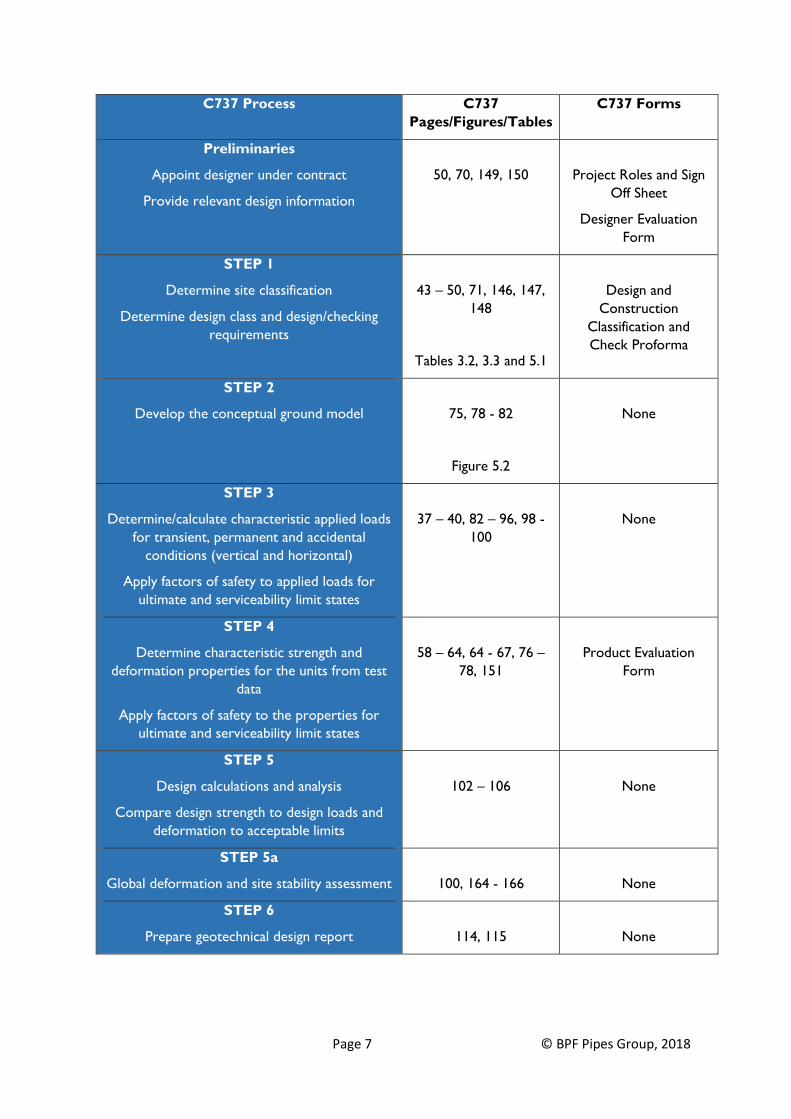
C737 Process Steps
Step 1 – Determine the qualifications of the designer along with the testing, analysis and design
checks that are required dependant on the site classification (0 to 3).
Step 2 – Prepare a conceptual ground model which summarises the critical factors relevant to the
design (geology, soil and tank parameters, tank geometry, etc.). This should be a diagrammatic
cross-section.
Step 3 – Determine the loads that are realistically likely to be applied to the tank. A conservative
approach is applied throughout C737 and engineering judgement may determine that some
assumptions are not applicable to a site (e.g., the assumption that a tank in a garden next to a drive
will be subject to HGV loads). Apply appropriate partial factors of safety to obtain the design loads.
Step 4 – Determine the characteristic strength and deformation properties for the geocellular units.
Manufacturers should provide sufficient information to allow designers to understand and analyse
the performance of the units. The parameters should be those that are declared by the
manufacturer. Apply appropriate partial factors of safety to obtain design properties.
Step 5 – Compare the design loads to the design strength. Assess elastic deformation under short-
term loads and permanent deformation under long-term loads.
Step 6 – Prepare a geotechnical design report. This does not have to be a long-winded report.
The purpose of the report is to communicate to those building the tank the critical aspects of the
design approach and assumptions made that they need to be aware of. The most effective form of
communication is a short one- or two-page summary of the information (including a diagrammatic
ground conceptual model).
Page 7 © BPF Pipes Group, 2018
C737 Process C737
Pages/Figures/Tables
C737 Forms
Preliminaries
Appoint designer under contract
Provide relevant design information
50, 70, 149, 150
Project Roles and Sign
Off Sheet
Designer Evaluation
Form
STEP 1
Determine site classification
Determine design class and design/checking
requirements
43 – 50, 71, 146, 147,
148
Tables 3.2, 3.3 and 5.1
Design and
Construction
Classification and
Check Proforma
STEP 2
Develop the conceptual ground model
75, 78 - 82
Figure 5.2
None
STEP 3
Determine/calculate characteristic applied loads
for transient, permanent and accidental
conditions (vertical and horizontal)
Apply factors of safety to applied loads for
ultimate and serviceability limit states
37 – 40, 82 – 96, 98 -
100
None
STEP 4
Determine characteristic strength and
deformation properties for the units from test
data
Apply factors of safety to the properties for
ultimate and serviceability limit states
58 – 64, 64 - 67, 76 –
78, 151
Product Evaluation
Form
STEP 5
Design calculations and analysis
Compare design strength to design loads and
deformation to acceptable limits
102 – 106
None
STEP 5a
Global deformation and site stability assessment
100, 164 - 166
None
STEP 6
Prepare geotechnical design report
114, 115
None

Page 8 © BPF Pipes Group, 2018
2.2 Accidental loading C737 requires the designer to consider routine loads (i.e., the standard load case) and the
performance of the tank under accidental loads. The accidental load analysis uses higher loads but
lower factors of safety than the standard load case. Examples of an accidental load are an HGV
entering a car park that is only designed for car traffic or materials being temporarily stockpiled on a
tank during construction when the tank should be fenced off to prevent this.
In this worked example, calculations are shown that analyse a standard load case. The same process
should also be repeated for the accidental load scenario using the accidental loads and appropriate
partial factors of safety.
2.3 Temporary construction situation In this worked example, it is assumed that the tank would not be subject to traffic during
construction until the final car park surfacing has been laid. It is also assumed it will not be trafficked
by cranes or cherry pickers. If the tank will be trafficked by construction traffic when the cover is
less than the final design and/or by heavier vehicles than those expected in service, a separate set of
calculations should be completed using appropriate loads and factors of safety.

Page 9 © BPF Pipes Group, 2018
3. Details for the worked example in this guide
The worked example in this guide is based on the information provided below.
Example site – BPF Towers
A tank is to be installed below a car park for a supermarket, at a depth of 2.4 m to the invert level of
the tank (or base of tank). There are no height barriers in the car park but warning signs will be
provided prohibiting HGVs from the car park area where the tank is situated. The cover over the
top of the tank to the top of the car park surfacing (finished ground level) is 1.2 m which is
consistent over the whole tank. The tank will be 30 m long by 10 m wide by 1.2 m high.
The tank will be an attenuation tank installed in level ground. The nearest building to the tank is 5.5
m away and the toe of a railway embankment is located 15 m from the tank. The tank will be
wrapped in a geomembrane (i.e., a waterproof liner). The site and tank layout is shown in Figure 1.
The scheme drawings showing the site layout, drainage layout, sections and details have been
provided to the Principal Designer along with the ground investigation report, which includes
information on the groundwater conditions.
The ground conditions at the tank site comprise:
• Made Ground – typically 1m thick and comprising medium dense black sandy GRAVEL of ash
and clinker.
• Glacial Till – typically 6 m thick and comprising firm to stiff dark grey silty CLAY with much
fine to coarse gravel.
• Coal Measures – not investigated but typically comprises a series of sandstones, siltstones,
mudstones and coal seams. Features that could affect tank stability such as shallow coal
workings or shafts are not expected.
Groundwater monitoring has shown that groundwater is not anticipated to be present above the
base of the tank at any point during the year.
The tank will be installed in an excavation that has a 0.5 m wide working space at the bottom and
with slopes battered back at 1 in 1. The excavation around the sides of the tank will be backfilled
with Class 6N Material (Manual of Contract Documents for Highway Works, Volume 1,
Specification for Highway Works). It is intended that once the tank is backfilled and constructed to
pavement level that construction traffic will pass over it but it is not in a location where cranes, etc.,
are likely to operate. The road/car park pavement construction will comprise 100 mm of asphalt
over 200 mm of Type 1 sub-base. The remaining depth of fill to the top of the tank will comprise
general granular fill material.
The tank will be provided with a vent consisting of a 100 mm pipe in a suitable location that is
accessible.
Inlet and outlet details and maintenance access are shown on the scheme general arrangement
drawing.
The geocellular units to be used in this example are manufactured by Mr Plastic Manufacturing
Company Limited. WaterBox 1 Units will be supplied. A 50-year design life has been specified for
the tank by the Client.

Page 10 © BPF Pipes Group, 2018
Figure 1 Example scheme general arrangement

Page 11 © BPF Pipes Group, 2018
4. Layout of the worked example in this guide
The layout of this guide in the following pages is shown below.
References to relevant pages or tables in C737 or The SuDS Manual are shown in bold
Explanation of the forms or calculations with
references to the relevant pages in C737 and The
SuDS Manual
Example of the completed form or calculation

Page 12 © BPF Pipes Group, 2018
5. Preliminaries
Prior to starting the design, the Project Roles and Sign Off Sheet and the Designer Evaluation Form
should be completed (as far as is possible at this stage).
5.1 Project Roles and Sign Off Sheet (Pages 50, 70, 149 C737)
The Project Roles and Sign Off Sheet identifies the main parties in the design and installation of a
geocellular tank. It will be a living document and should be first used to record the details of the
designer of the tank. As the project progresses, the other parties can be added as they become
known. A copy of the sheet from Appendix A1 C737 is provided on the adjacent page.
The Client is the person who is commissioning the design and construction of the project.
The Principal Designer is the organisation that is responsible for the structural and geotechnical
design of the tank. This may be the consultant that has designed the overall drainage system or it
may be delegated to a specialist sub-consultant or supplier/manufacturer. In this example, it is
Drainage Design Consultant Limited.
The Principal Contractor is that organisation designated under the CDM Regulations. In this
example the design is being completed before tendering and, therefore, the Principal Contractor is
not yet known.
The Geocellular Manufacturer/Supplier is the organisation that supplies the tank units. If this
changes during the development of the project (for example, if the Principal Contractor proposes an
alternative system to that shown in the design or a minimum performance specification has been
provided by the designer) then this form should be updated. In this example, it is Mr Plastic
Manufacturing Company Limited.
Site classification assessment is based on the results of the Design and Construction Classification
and Check Proforma (see the next section of this guide). In this example, the results of completing
the Design and Classification and Check Proforma indicate the site is Class 1.

Page 13 © BPF Pipes Group, 2018
X

Page 14 © BPF Pipes Group, 2018
5.2 Designer Evaluation Form (Page 150 C737)
This form is used to summarise the relevant design information that has been passed to the Principal
Designer by the Client or other party (e.g., main design consultant).
The design information for the worked example is summarised in the form on the adjacent page.
Design function – in this example, the tank is an attenuation tank.
End surface use – in this example, the tank will be below a supermarket car park which can be
defined as a ‘car park, general, no height access restrictions’. Judgement should be applied into
which category a site fits. Careful consideration of likely access by HGVs is required, as factors
other than the height of barriers may restrict access (e.g., very tight corners, width of access route,
earth berms or planting around landscaped areas, etc.).
Background information provided to the manufacturer – in this example, it is assumed that
all necessary information has been provided. If information is missing then any assumptions made in
the design or caveats as to its application should be clearly stated. In this case, the dimensions for
the tank are shown as 30 m x 10 m x 1.2 m. The ground is level and so the maximum and minimum
depth of cover is the same at 1.2 m and the finished ground level (FGL) variation is zero.
Volume of installation – this is termed ‘net volume’ in the C737 Design Evaluation Form. The
usual understanding of the term ‘net volume’ would be the storage volume required, with ‘gross
volume’ being the total volume of the tank considering porosity. In the form there is no space to
include a value for porosity, therefore, the volume of installation is simply the volume of the tank.
This has no practical significance to the design.
Construction details provided to the manufacturer – it is important that any construction
details assumed or required in the design are stated. For example, in this case the assumption of the
use of Class 6N backfill will affect the angle of friction and hence the applied lateral pressure on the
side of the tank. These factors should also be carried forward to the geotechnical design report.
Details of maintenance access points to inspect or clean the tank, inlets and outlets and ventilation of
the tank are shown on the scheme general arrangement drawings.

Page 15 © BPF Pipes Group, 2018

Page 16 © BPF Pipes Group, 2018
6. Step 1: Determine site classification, design class and
design/checking requirements
(Pages 43 - 50, 146, 147 C737)
6.1 Worked example The purpose of the Site Classification Proforma is to distinguish the level of design and checking that is
required. This can range from simple sites that need very little design input to complex sites or sites
where the consequences of failure are severe where a high degree of analysis and checking may be
necessary.
Experience shows that sudden catastrophic collapse of geocellular structures is not likely to occur
and if collapse does occur it would be a slow progressive mechanism. This should be considered
when assessing the consequences of failure.
The Site Classification Proforma is completed and the site and installation together will achieve a score.
The score is used to define the classification of the site and tank (Table 3.2, Page 48 C737).
The classification of the site and tank determines the level of design checking that is necessary
(Table 3.3, Page 49 C737).
In this example, the site is not within any zones of influence from slopes, retaining walls or
foundations. The tank is 5.5 m from the nearest building foundation and the depth, h, is 2.4 m. The
limit for the zone of influence is shown on the proforma as 2 m + h = 4.4 m. Therefore, the tank is
not within the zone of influence of the foundation.
The tank is 15 m from a railway embankment. The limit for the zone of influence is shown on the
proforma as 10 m + h = 12.4 m. Therefore, the tank is not within the zone of influence of the
embankment.
1. Type of site - The site in this example is a supermarket and, therefore, is a commercial
application. Score = 10.
The single domestic dwelling only applies to small soakaway or attenuation tanks for a single private
house.
2. Use - The tank will be an attenuation tank. Score = 5.
The BPF Pipes Group considers that the use of the tank as attenuation or soakaway makes no
difference to the level of risk in the structural design. For tanks above the groundwater table, the
risks and consequences associated with structural failure are the same for both an attenuation tank
or a soakaway and a score of 5 can be used. However, if attenuation tanks are constructed below
the water table the risk of failure is higher and so a higher score of 10 is applied. It is preferable to
construct all tanks above the water table, wherever possible.
Assign a score based on the level of risk or consequences of failure with respect to the structural
design. Attenuation and grey/rainwater storage are given a score of 5 in the proforma rather than
10. For other applications, the score does not have to be 15 as stated on the proforma.

Page 17 © BPF Pipes Group, 2018
X 5
X 5 X depends on risk

Page 18 © BPF Pipes Group, 2018
3. Pre-design/construction information held – In this example, it is assumed that all
information is available from the Principal Designer. Score = 0.
The information is important for design. Geological mapping, a desk study and groundwater data are
usually included in a basic site investigation along with information on soil types from boreholes,
probe holes or trial pits.
The information listed is necessary to identify the design hazards (e.g., the overall site development
plan will show if the tank is near foundations and the ground and groundwater information allows
the pressure on the side of the tank to be estimated).
4. Topography/retaining walls/stockpiles/foundations – In this example, the site is on level
ground. Score = 0.
If the tank is near anything that could impose additional load on the sides or top, give a score of 30.
If the tank collapsed and could cause unacceptable movement or collapse of foundations, slopes,
retaining walls, etc., then give a score of 60.
5. Installation development location and use – In this example, the tank is in a car park
(general) with no height access restrictions. Score = 20.
Choose one of the locations/uses identified in the table on the proforma. Judgement will be
required to assign the use of the site to one of the categories. The basic principle is that the greater
the consequences of failure the higher the score.
6. Depth of installation In this example the tank is 2.4 m deep (i.e., between 1 m and 3 m to
base). Score = 5.
In this example, the tank has greater than 1m cover and is subject to traffic. Score = 15.
The worst of the two scores is applied in the scoring system otherwise double counting can occur.
In this case, the worst score is given by the cover and traffic. Score = 15.
7. Construction phase – In this example, there is no construction access or stockpiles over the
tank and an exclusion zone will be implemented. Score = 0.
If several of these factors apply, then use the worst-case value to determine the score to avoid
doubling up.
Consider each site individually to assess if any other site-specific factors could affect the score.
Assessment total score - Add up the individual scores. For this example, Total = 50.
Using Table 3.2 C737 for this example the Site Classification is 1.

Page 19 © BPF Pipes Group, 2018
50

Page 20 © BPF Pipes Group, 2018
6.2 Results of the site classification and implications In this example, the site is classified as Class 1 with the following implications:
• Undertake design checks for vertical distributed and concentrated loading.
• Check adequacy of cover over units to distribute wheel loads.
• Check uplift, if appropriate (for tanks below groundwater).
• Assess earth pressures using active pressure coefficient.
• Use standard test methods and data for the properties of the geocellular units.
These checks are explained in the following worked example.
In this example, the Class 1 requirements will mean that the design checks are completed by a
competent building professional with relevant industry experience. An Incorporated or Chartered
Engineer is to oversee the design checks. Drainage Design Consultants Limited (the company
responsible for the design in this example) should confirm that these requirements have been met.
6.3 Generic classification system for routine sites A generic classification system for different zones has been prepared for sites where the tank design
will be routine and there are no special circumstances (i.e., the tanks are not unusually deep or
shallow or are not within the zone of influence of slopes, buildings, etc.). The classification is
provided in Table 1 of this guide. This is based on the following traffic zones (further information on
the zones is provided in Appendix B of this guide).
A Anywhere that vehicle access is not possible (e.g., due to fences or barriers, road layout
or topography).
B Anywhere that only cars can access due to physical constraints.
C Anywhere that HGVs will only access as an “accidental load” (i.e., not regular HGV traffic,
for example, vehicle overrun on a verge at the back of a footway).
D Anywhere that is subject to limited HGV traffic at very low speed (<15 mph) such as fire
tenders and refuse trucks.
E Everywhere else (assumed to be subject to regular unrestricted HGV traffic). This
category is split into three sub-categories depending on the type of HGV loading that is
expected (E1 to E3). E1 is for areas where HGVs will be regular and moving at low
speeds such as lorry parks and loading bays. E2 would cover some estate roads in
residential developments and E3 would cover trunk roads and motorways. In the latter
case in the running lanes of motorways (including the occasional hard shoulder on Smart
Motorways), specific assessment of the special vehicle loads should be undertaken to the
requirements of Highways England.

Page 21 © BPF Pipes Group, 2018
Table 1 Generic Classification
Traffic
zone
General
description
Type of site
Sco
re
Use
Sco
re
Information
Sco
re
Topography
Sco
re
Location
Sco
re
Depth
to base
Sco
re
Cover (see
note at
base of
table)
Sco
re
Construction
phase
Sco
re
Classification Testing
requirements
Recommended
actions/roles
(Table 3.2 C737)
Design
requirements
(Table 3.3 C737)
Checking
requirements
(Table 3.2 C737) Total
score
Class
A No vehicular
access
Commercial 10 Attenuation 5
Ass
um
e a
ll re
leva
nt
info
rmat
ion is
avai
lable
0 Level ground 0 Equivalent to
parkland
0 1 m to 3
m
5 0.3 m to 2 m
landscaped
10
Ass
um
e s
om
e c
onst
ruct
ion p
lant
pas
sing
ove
r
20 50 1 Long-term creep
rupture and short-
term tests (300 mm
diameter and full
plate)
Simple design
calculations by
competent building
professional with
relevant industry
experience
Check units have
sufficient strength to
support vertical loads
(distributed and
concentrated).
Check cover to units
is sufficient to
distribute
concentrated loads
and to prevent
flotation. Assess
earth and water
pressure on sides
using standard
methods and
assuming active earth
pressure coefficients
apply
Simple design checks
to be undertaken by
competent building
professional.
Independent check by
another engineer
who may be from the
same team
(Incorporated or
Chartered Engineer
to oversee checks)
B Car access only Commercial 10 Attenuation 5 0 Level ground 0 Equivalent to
car park light
use
15 1 m to 3
m 5 1 m to 2 m
trafficked
15 20 70 1
C Accidental
HGV access
Commercial 10 Attenuation 5 0 Level ground 0 Equivalent to
car park
general
20 1 m to 3
m 5 1 m to 2 m
trafficked 15 20 75 1
D Limited HGV
traffic at low
speed
Commercial 10 Attenuation 5 0 Level ground 0 Low speed
roads
30 1 m to 3
m 5 1 m to 2 m
trafficked 15 20 85 2 Long-term creep
rupture and short-
term tests (300 mm
diameter and full
plate)
Design by Chartered
Civil Engineer with 5
years ‘post chartered’
specialist experience
in ground engineering
Check units as above.
Consider allowable
movements and
assessment of
manufacturer’s data.
Consider creep
deformation. Detailed
assessment of
construction
activities.
Design overseen by
Chartered Civil
Engineer with 5 years
‘post chartered’
specialist experience.
Category 2 check by
an Engineer who
must be independent
of the design team
but can be from the
same organisation
E1 Regular HGV
traffic at low
speeds
Commercial 10 Attenuation 5 0 Level ground 0 HGV park 30 1 m to 3
m 5 1 m to 2 m
trafficked 15 20 85 2
E2 and
E3
All other
locations. High
speed HGV
traffic
Commercial 10 Attenuation 5 0 Level ground 0 Equivalent to
full highway
loading
80 1 m to 3
m 5 1 m to 2 m
trafficked 15 20 135 3 Long-term and short-
term tests as above
plus cyclic loading
tests (fatigue test).
Full-scale pavement
tests if less than 1 m
cover to tank
Design by Chartered
Civil Engineer with
Geotechnical Advisor
status
As above plus
assessment of fatigue
and cyclic loading and
detailed assessment
of deformations.
Numerical modelling
required
Senior Specialist
Geotechnical
Engineer with
Geotechnical Advisor
status should be
appointed to oversee
design process, likely
complex modelling
and testing required.
Category 3 check by
an Engineer from a
separate organisation
to that of the
designer.
NOTES: Assume all locations
are “commercial”
Assume attenuation
is worst case. Note -
there is no reason
why attenuation is
greater risk than
soakaway so score
for soakaway has
been used
Assume for this first
stage, level ground and
outside zone of
influence of walls, etc.
Assume >1 m but
less than 2 m = 0.
Not explicitly
stated
Assume the tank is not
below groundwater
table
Assume tank is
outside zone of
influence of any
structure etc. i.e.
Zone 4
Assumes units are
not prone to
excessive bending or
instability when
subject to shear loads
or other uneven
loading (units
assembled on site
from plates require
specific shear testing)

Page 22 © BPF Pipes Group, 2018
7. Step 2: Develop the conceptual ground model
(Pages 78 - 82 C737)
The purpose of the conceptual ground model is to describe the tank installation and the surrounding
ground. It will also include any slopes or nearby structures that will influence the design. The
conceptual ground model forms the basis of the design analysis and calculations.
The best way to present the ground model is for the designer to draw up a cross-section of the
proposed tank installation showing the tank, backfill details, excavation limits, backfill materials,
nearby slopes or walls, etc. The properties of the tank installation and the surrounding ground
should be summarised on the ground model.
The key items are:
• Ground level profile over and adjacent to tank.
• Depth of cover over top of tank.
• Depth to base of tank.
• Geological profile of ground around the tank.
• Soil or rock properties of the surrounding ground and proposed backfill.
• Extent of excavation for the tank.
• Strength and deformation properties of the proposed tank.
• Nearby structures, slopes or other features that may influence the design and performance
of the tank.
The conceptual ground model for the site and tank being considered in this worked example is
provided in Figure 2.

Page 23 © BPF Pipes Group, 2018
Figure 2 Example conceptual ground model
Ground properties
Stratum Typical
thickness
Unit weight Effective angle of
friction
Made Ground (medium dense black
sandy GRAVEL of ash and clinker)
1.0m 18kN/m3 32o
Glacial Till (firm to stiff dark grey silty
sandy CLAY with much fine to coarse
gravel)
6.0m 20kN/m3 28o
Coal Measures (not investigated).
Geological map indicates series of
mudstone, siltstone, sandstone and
coal seams. No workings
100m+ n/a n/a
Class 6N backfill to Specification for
Highway Works
-- 18kN/m3 36o
Class 1 General granular fill to
Specification for Highway Works
-- 20kN/m3 32o
Manufacturer declared values for properties of geocellular
tank
Unit Mr Plastic Manufacturing Company Ltd, Waterbox 1
Vertical Horizontal
Ultimate strength
(short-term mean
value)
440kN/m2 97kN/m2
Characteristic
strength (long-term,
50 years)
124kN/m2 27kN/m2
Design strength (50
years)
83kN/m2 18kN/m2
Reference strength
(20 years)
85.5kN/m2 18.5kN/m2
See Product Evaluation Form for further information (C737 Page 151)
Page 24 © BPF Pipes Group, 2018
8. Step 3: Determine characteristic loads and apply partial
factors to give design loads
8.1 Loads The following loads will be calculated:
Step 3.1: Vertical characteristic load from backfill and surcharge.
Step 3.2: Vertical characteristic traffic loading.
Step 3.3: Lateral characteristic load from earth pressure and groundwater.
Step 3.4: Lateral characteristic load from wheel loads adjacent to tank.
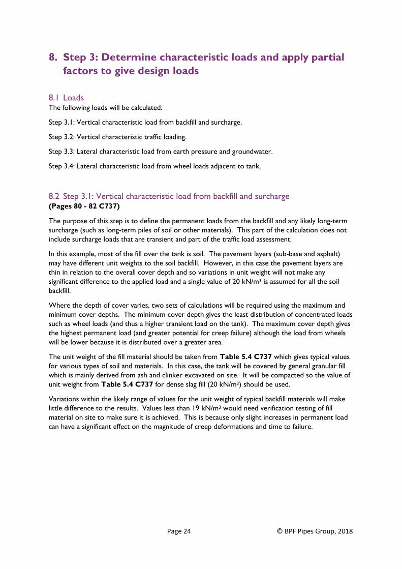
8.2 Step 3.1: Vertical characteristic load from backfill and surcharge (Pages 80 - 82 C737)
The purpose of this step is to define the permanent loads from the backfill and any likely long-term
surcharge (such as long-term piles of soil or other materials). This part of the calculation does not
include surcharge loads that are transient and part of the traffic load assessment.
In this example, most of the fill over the tank is soil. The pavement layers (sub-base and asphalt)
may have different unit weights to the soil backfill. However, in this case the pavement layers are
thin in relation to the overall cover depth and so variations in unit weight will not make any
significant difference to the applied load and a single value of 20 kN/m3 is assumed for all the soil
backfill.
Where the depth of cover varies, two sets of calculations will be required using the maximum and
minimum cover depths. The minimum cover depth gives the least distribution of concentrated loads
such as wheel loads (and thus a higher transient load on the tank). The maximum cover depth gives
the highest permanent load (and greater potential for creep failure) although the load from wheels
will be lower because it is distributed over a greater area.
The unit weight of the fill material should be taken from Table 5.4 C737 which gives typical values
for various types of soil and materials. In this case, the tank will be covered by general granular fill
which is mainly derived from ash and clinker excavated on site. It will be compacted so the value of
unit weight from Table 5.4 C737 for dense slag fill (20 kN/m3) should be used.
Variations within the likely range of values for the unit weight of typical backfill materials will make
little difference to the results. Values less than 19 kN/m3 would need verification testing of fill
material on site to make sure it is achieved. This is because only slight increases in permanent load
can have a significant effect on the magnitude of creep deformations and time to failure.

Page 25 © BPF Pipes Group, 2018
Project: BPF Towers Page: 1
Description: Example design
Designer: BPF Pipes Group Date: Feb 2017
Characteristic load from backfill and surcharge (permanent)
Depth of fill over top of tank, Z1 = 1.2 m
Unit weight of fill, γ = 2o kN / m3
Characteristic permanent distributed load, QckP = Z1 x γ
= 1.2 x 20 = 24 kN / m2
Checker: BPF Pipes Group Date: 8/03/2017
Page 26 © BPF Pipes Group, 2018
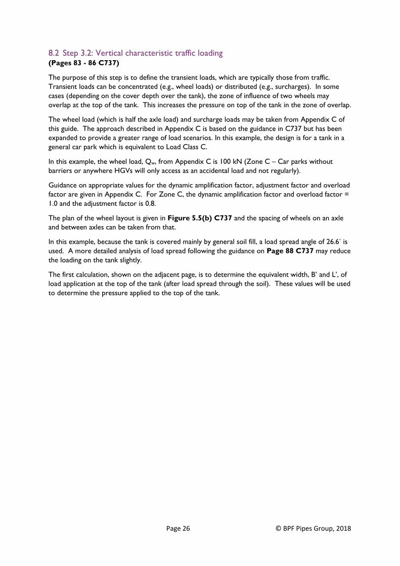
8.2 Step 3.2: Vertical characteristic traffic loading (Pages 83 - 86 C737)
The purpose of this step is to define the transient loads, which are typically those from traffic.
Transient loads can be concentrated (e.g., wheel loads) or distributed (e.g., surcharges). In some
cases (depending on the cover depth over the tank), the zone of influence of two wheels may
overlap at the top of the tank. This increases the pressure on top of the tank in the zone of overlap.
The wheel load (which is half the axle load) and surcharge loads may be taken from Appendix C of
this guide. The approach described in Appendix C is based on the guidance in C737 but has been
expanded to provide a greater range of load scenarios. In this example, the design is for a tank in a
general car park which is equivalent to Load Class C.
In this example, the wheel load, Qw, from Appendix C is 100 kN (Zone C – Car parks without
barriers or anywhere HGVs will only access as an accidental load and not regularly).
Guidance on appropriate values for the dynamic amplification factor, adjustment factor and overload
factor are given in Appendix C. For Zone C, the dynamic amplification factor and overload factor =
1.0 and the adjustment factor is 0.8.
The plan of the wheel layout is given in Figure 5.5(b) C737 and the spacing of wheels on an axle
and between axles can be taken from that.
In this example, because the tank is covered mainly by general soil fill, a load spread angle of 26.6° is
used. A more detailed analysis of load spread following the guidance on Page 88 C737 may reduce
the loading on the tank slightly.
The first calculation, shown on the adjacent page, is to determine the equivalent width, B’ and L’, of
load application at the top of the tank (after load spread through the soil). These values will be used
to determine the pressure applied to the top of the tank.

Page 27 © BPF Pipes Group, 2018
Project: BPF Towers Page: 2
Description: Example design
Designer: BPF Pipes Group Date: Feb 2017
Characteristic load from traffic (transient)
Input Values:
Characteristic surcharge pressure for traffic, gK = 5.5 kN / m2
Wheel load, QW = 100 kN
Wheel contact width, B = 0.4 m
Wheel contact length, L = 0.4 m
Dynamic amplification factor, DAF = 1.0
Adjustment factor = 0.8
Overload factor, OLF = 1.0
Distance between centreline of adjacent axles, dWL = 1.2 m
Distance between centreline of wheels on one axle, dWB = 2.0 m
Load spread angle through pavement and fill, θ = 26.6°
Calculate:
Extent of load spread at top of tank
Equivalent width B’ = (2 x Z1 x TANθ) + B
B’ = (2 x 1.2 x TAN 26.6°) + 0.4 = 1.6 m
Equivalent length L’ = (2 x Z1 x TANθ) + L
L’ = (2 x 1.2 x TAN 26.6°) + 0.4 = 1.6 m
Checker: BPF Pipes Group Date: 8/03/2017

Page 28 © BPF Pipes Group, 2018
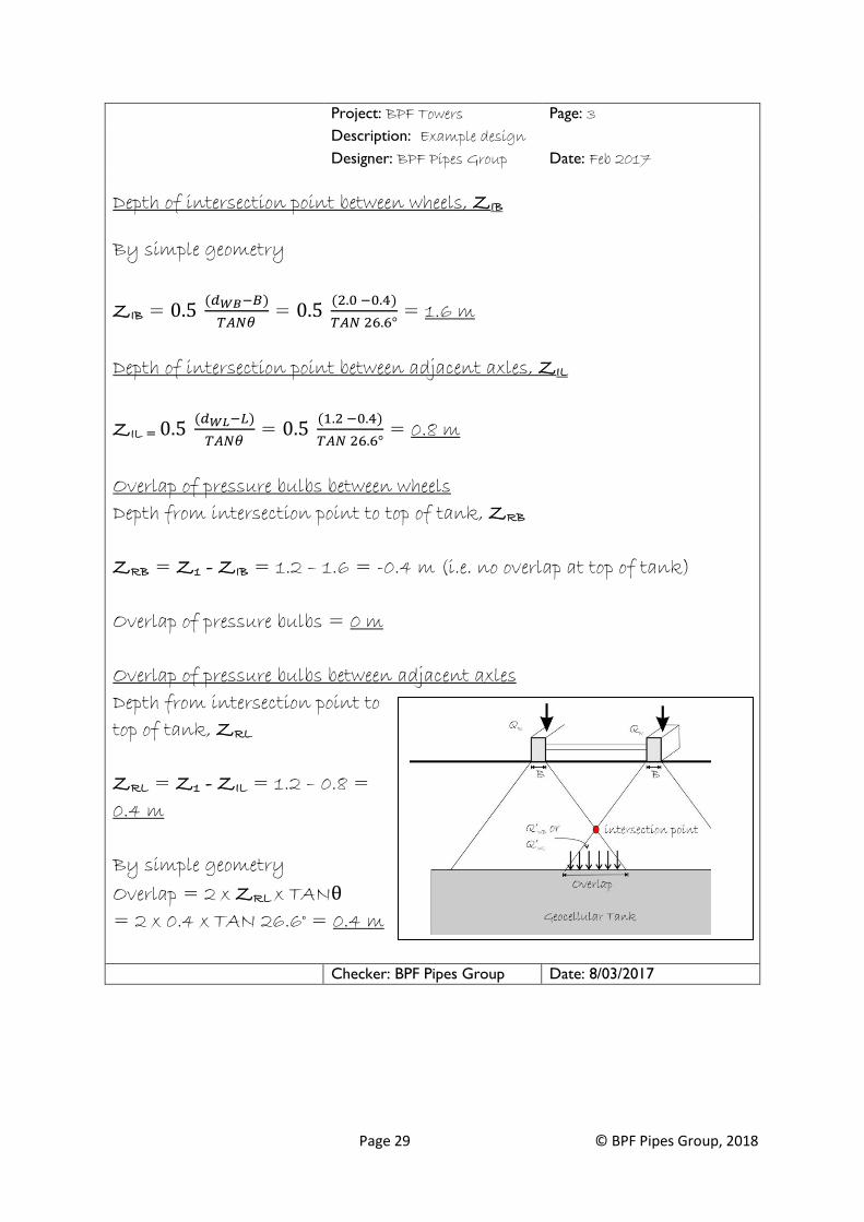
The calculation shown on the adjacent page is to determine the depth to the intersection point of
the load spread lines from adjacent wheels. The depth from the intersection point to the top of the
tank is then calculated. This is all based on simple geometrical analysis and allows the zone of
overlap to be determined.
If the point of intersection is above the tank, then the applied pressure in the overlap area is twice
that from a single wheel.
The load applied to the top of the tank from a single wheel is based on the spread angle and the
depth to the top of the tank.
Page 29 © BPF Pipes Group, 2018
Project: BPF Towers Page: 3
Description: Example design
Designer: BPF Pipes Group Date: Feb 2017
Depth of intersection point between wheels, ZIB
By simple geometry
ZIB = 0.5 (𝑑𝑊𝐵−𝐵)
𝑇𝐴𝑁𝜃 = 0.5
(2.0 −0.4)
𝑇𝐴𝑁 26.6° = 1.6 m
Depth of intersection point between adjacent axles, ZIL
ZIL = 0.5 (𝑑𝑊𝐿−𝐿)
𝑇𝐴𝑁𝜃 = 0.5
(1.2 −0.4)
𝑇𝐴𝑁 26.6° = 0.8 m
Overlap of pressure bulbs between wheels
Depth from intersection point to top of tank, ZRB
ZRB = Z1 - ZIB = 1.2 – 1.6 = -0.4 m (i.e. no overlap at top of tank)
Overlap of pressure bulbs = 0 m
Overlap of pressure bulbs between adjacent axles
Depth from intersection point to
top of tank, ZRL
ZRL = Z1 - ZIL = 1.2 – 0.8 =
0.4 m
By simple geometry
Overlap = 2 x ZRL x TANθ
= 2 x 0.4 x TAN 26.6° = 0.4 m
Checker: BPF Pipes Group Date: 8/03/2017

Page 30 © BPF Pipes Group, 2018
The calculation shown on the adjacent page uses the load spread and overlap from the previous
sheets to calculate the wheel load on the tank for a single wheel and in the overlap zone.
The total characteristic load from traffic is the sum of the load applied at the top of the tank from
the wheel loads plus the transient surcharge load.

Page 31 © BPF Pipes Group, 2018
Project: BPF Towers Page: 4
Description: Example design
Designer: BPF Pipes Group Date: Feb 2017
Wheel load on tank, no overlap, Q’W
Q’W = 𝑄𝑤 𝑥 𝐷𝐴𝐹 𝑥 𝐴𝑑𝑗𝑢𝑠𝑡𝑚𝑒𝑛𝑡 𝐹𝑎𝑐𝑡𝑜𝑟 𝑥 𝑂𝐿𝐹
𝐵′𝑥 𝐿′=
100 𝑥 1.0 𝑥 0.8 𝑥 1.0
1.6 𝑥 1.6 = 31.25 kN / m2
Wheel load on tank, zone of overlap adjacent to axles, Q’wL
Q’WL = 2 x Q’W = 2 x 31.25 = 62.5 kN / m2
In this case, Q’WB is the same as Q’W because there is no overlap in that
direction.
Total characteristic load from traffic, QckT
QckT = Wheel load + surcharge load
Use maximum value of wheel load from Q’W, Q’WL and Q’WB
QckT =(62.5 + 5.5) kN / m2 = 68.0 kN / m2
Checker: BPF Pipes Group Date: 8/03/2017
Page 32 © BPF Pipes Group, 2018
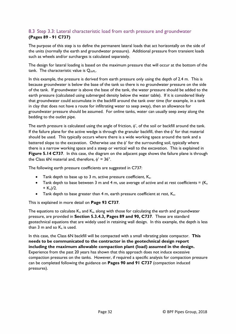
8.3 Step 3.3: Lateral characteristic load from earth pressure and groundwater (Pages 89 - 91 C737)
The purpose of this step is to define the permanent lateral loads that act horizontally on the side of
the units (normally the earth and groundwater pressure). Additional pressure from transient loads
such as wheels and/or surcharges is calculated separately.
The design for lateral loading is based on the maximum pressure that will occur at the bottom of the
tank. The characteristic value is QckPL.
In this example, the pressure is derived from earth pressure only using the depth of 2.4 m. This is
because groundwater is below the base of the tank so there is no groundwater pressure on the side
of the tank. If groundwater is above the base of the tank, the water pressure should be added to the
earth pressure (calculated using submerged density below the water table). If it is considered likely
that groundwater could accumulate in the backfill around the tank over time (for example, in a tank
in clay that does not have a route for infiltrating water to seep away), then an allowance for
groundwater pressure should be assumed. For online tanks, water can usually seep away along the
bedding to the outlet pipe.
The earth pressure is calculated using the angle of friction, ’, of the soil or backfill around the tank.
If the failure plane for the active wedge is through the granular backfill, then the’ for that material
should be used. This typically occurs where there is a wide working space around the tank and a
battered slope to the excavation. Otherwise use the ’ for the surrounding soil, typically where
there is a narrow working space and a steep or vertical wall to the excavation. This is explained in
Figure 5.14 C737. In this case, the diagram on the adjacent page shows the failure plane is through
the Class 6N material and, therefore, ’ = 36°.
The following earth pressure coefficients are suggested in C737:
• Tank depth to base up to 3 m, active pressure coefficient, Ka.
• Tank depth to base between 3 m and 4 m, use average of active and at rest coefficients = (Ka
+ Ko)/2.
• Tank depth to base greater than 4 m, earth pressure coefficient at rest, Ko.
This is explained in more detail on Page 93 C737.
The equations to calculate Ko and Ka, along with those for calculating the earth and groundwater
pressure, are provided in Section 5.3.4.3, Pages 89 and 90, C737. These are standard
geotechnical equations that are widely used in retaining wall design. In this example, the depth is less
than 3 m and so Ka is used.
In this case, the Class 6N backfill will be compacted with a small vibrating plate compactor. This
needs to be communicated to the contractor in the geotechnical design report
including the maximum allowable compaction plant (load) assumed in the design.
Experience from the past 20 years has shown that this approach does not induce excessive
compaction pressures on the tanks. However, if required a specific analysis for compaction pressure
can be completed following the guidance on Pages 90 and 91 C737 (compaction induced
pressures).

Page 33 © BPF Pipes Group, 2018
Project: BPF Towers Page: 5
Description: Example design
Designer: BPF Pipes Group Date: Feb 2017
Characteristic lateral load from earth pressure and groundwater, QckPL
Depth of base of tank = ZB = 2.4 m
Effective angle of friction of backfill, ϕ’ = 36 °
Page 94 of C737, Fig 5.14
Active wedge forms at 45°- ϕ′
2 = 45°-
36
2 = 27°
Active wedge forms in Class 6N backfill material
Therefore, use ϕ’ = 36 ° in design
Φ’BD = 36 °
Page 93 of C737, depth is less than 3 m so use Ka, active pressure
coefficient
Ka = 1−𝑆𝐼𝑁ϕ′
1+𝑆𝐼𝑁 ϕ′ =
1−𝑆𝐼𝑁 36°
1+𝑆𝐼𝑁 36° = 0.26
QckPL = Ka x γ x ZB = 0.26 x 18 x 2.4 = 11.23 kN / m2
Checker: BPF Pipes Group Date: 8/03/2017

Page 34 © BPF Pipes Group, 2018
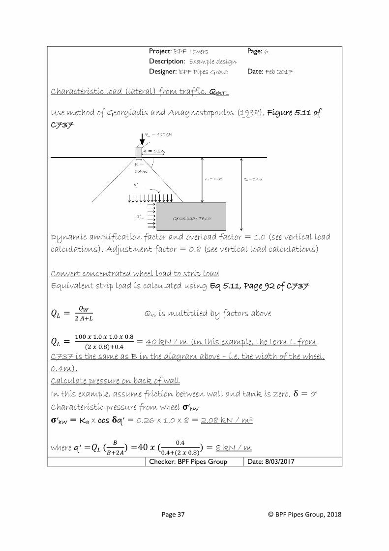
8.4 Step 3.4: Lateral characteristic load from wheel loads adjacent to tank (Pages 92 - 93 C737)
The purpose of this step is to define the horizontal loads on the side of the tank that are caused by
vehicle wheels located adjacent to the tank. The load is transmitted through the soil onto the side
of the tank.
In this example, the approach described by Georgiadis and Anagnostopoulos (1998)1 is used. This is
explained in Figure 5.11(b) C737. For simplicity, the wheel load is treated as a strip load equal to
the width of a wheel and is assumed to be continuous along the wall. This is conservative but not
excessively so and simplifies the analysis.
The applied pressure determined using this approach will vary with distance of the wheel from the
tank. The critical distance that results in the maximum pressure at the top of the tank has first to be
determined, prior to completing the Georgiadis and Anagnostopoulos analysis.
To do this the pressure distribution from the wheel is assumed to be a line load (or knife edge load).
In this example, it has been derived from the wheel load using Equation 5.11 from Page 92
C737. The applied pressure is calculated for each distance from the back of the wall using a
Boussinesq stress analysis (see Figure 3 and the equation below). This makes no allowance for the
soil properties. It does, however, give an indication of the likely dissipation of lateral loads from the
wheel in the soil above the top of the tank wall.
Figure 3 Derivation of pressure on side of tank from line load
The graph on the adjacent page has been derived using this approach, assuming the wheel load in this
example is 100 kN/m2 applied over a 400 mm by 400 mm contact area (as defined for Zone C in
Appendix B of this guide). The load is multiplied by the appropriate adjustment, dynamic and
1 Georgiadis M and Anagnostopoulos C (1998). Lateral Pressure on Sheet Pile Walls due to Strip Load. Journal of Geotechnical and Geoenvironmental Engineering Vol 124 Issue 1 January 1998. ASCE pp95 – 98.

Page 35 © BPF Pipes Group, 2018
overload factors from the previous sheets. The critical distance, A, at which the greatest pressure is
applied (at the level of the top of the tank) can then be determined.
The graph for this example is shown below. It is used to determine the critical distance for the
wheel load from the tank for the design cover depth. In this example, the top of the tank is at 1.2 m
depth and the maximum pressure occurs when the wheel is 0.8 m from the tank (i.e., A= 0.8 m).
This distance, A, must not exceed the cover depth of the tank.
In the equation above, the factor 2 allows for a flexible wall as explained in Foundation Analysis and
Design (J E Bowles, 4th Edition, McGraw-Hill International, 1998). Geocellular tanks are considered
to be flexible.
Figure 4 Variation of pressure on side of tank from wheel load for this example

Page 36 © BPF Pipes Group, 2018
Once the distance, A, has been determined using the Boussinesq analysis, the pressure on the side of
the tanks is calculated using Georgiadis and Anagnostopoulos (1998) as shown on the adjacent page.
In this example, the friction between the wall and the backfill is taken as zero. This is conservative
and if there is sufficient information about the interface friction for the geotextile or geomembrane
that is to be used, then an allowance may be made for friction.
In this case, the active earth pressure coefficient, Ka, is used as described previously. See the
previous permanent lateral load calculations (from earth pressure and groundwater) for a discussion
about the appropriate earth pressure coefficient to use.
Page 37 © BPF Pipes Group, 2018
Project: BPF Towers Page: 6
Description: Example design
Designer: BPF Pipes Group Date: Feb 2017
Characteristic load (lateral) from traffic, QckTL
Use method of Georgiadis and Anagnostopoulos (1998), Figure 5.11 of
C737
Dynamic amplification factor and overload factor = 1.0 (see vertical load
calculations). Adjustment factor = 0.8 (see vertical load calculations)
Convert concentrated wheel load to strip load
Equivalent strip load is calculated using Eq 5.11, Page 92 of C737
𝑄𝐿 = 𝑄𝑊
2 𝐴+𝐿 QW is multiplied by factors above
𝑄𝐿 = 100 𝑥 1.0 𝑥 1.0 𝑥 0.8
(2 𝑥 0.8)+0.4 = 40 kN / m (in this example, the term L from
C737 is the same as B in the diagram above – i.e. the width of the wheel,
0.4m).
Calculate pressure on back of wall
In this example, assume friction between wall and tank is zero, δ = 0°
Characteristic pressure from wheel σ’hW
σ’hW = Ka x cos δq’ = 0.26 x 1.0 x 8 = 2.08 kN / m2
where q’ =𝑄𝐿 (𝐵
𝐵+2𝐴) =40 𝑥 (
0.4
0.4+(2 𝑥 0.8)) = 8 kN / m
Checker: BPF Pipes Group Date: 8/03/2017

Page 38 © BPF Pipes Group, 2018
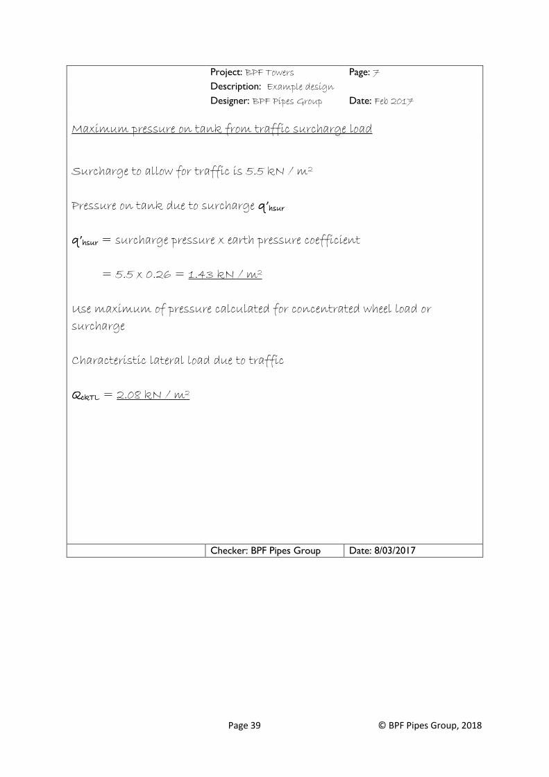
On the adjacent page, the pressure from the transient surcharge (traffic surcharge load) is calculated.
The equation used is from standard earth pressure theory:
Lateral pressure = surcharge pressure x earth pressure coefficient.
The maximum value of pressure from either the wheel load (previous sheet) or the transient
surcharge (this sheet) is used in the design to estimate pressure on the side of the tank from traffic.
There is normally no need to carry out a specific analysis of braking forces from vehicles
approaching a tank in a direction that is perpendicular to the side (as suggested on Page 89, C737).
The advice in C737 is based on the design of bridge decks and abutments where such loads are
transferred into the structure. It is highly conservative when applied to geocellular tanks buried in
the ground. Appendix D provides evidence to demonstrate that analysing braking forces from
vehicles moving towards a tank is not appropriate where the cover over tanks is greater than 0.6 m
in car parks and 1m where HGVs are travelling.
Page 39 © BPF Pipes Group, 2018
Project: BPF Towers Page: 7
Description: Example design
Designer: BPF Pipes Group Date: Feb 2017
Maximum pressure on tank from traffic surcharge load
Surcharge to allow for traffic is 5.5 kN / m2
Pressure on tank due to surcharge q’hsur
q’hsur = surcharge pressure x earth pressure coefficient
= 5.5 x 0.26 = 1.43 kN / m2
Use maximum of pressure calculated for concentrated wheel load or
surcharge
Characteristic lateral load due to traffic
QckTL = 2.08 kN / m2
Checker: BPF Pipes Group Date: 8/03/2017
Page 40 © BPF Pipes Group, 2018
8.5 Step 3.5: Partial factors of safety for loads and soil properties (Pages 99 - 100 C737)
Partial factors applied to loads
The purpose of this step is to determine the appropriate partial factors of safety that should be
applied to the characteristic loads or soil properties to arrive at design loads. The partial factors
applied to the properties of the geocellular units are explained in Section 9 of this guide.
Load factors for ultimate and serviceability states are provided in Table 5.9 C737 and those used in
this example are shown on the adjacent page. For lateral loads, Combination 1 in EC7 is assumed
for routine design to assess the resistance of the tanks to lateral pressure. Combination 2 would be
applicable for global stability checks such as slope stability analysis, where this is required. Note that
there may be instances where Combination 2 in EC7 gives the worst-case pressure on the tank (e.g.,
if there are large variable surcharge loads and the retained soil has a high angle of friction).
Unfavourable loads are those that adversely affect the tank (e.g., the permanent load from the
weight of soil on top of the tank, traffic loads and the pressure from earth on the sides of the tank).
Favourable loads are those that are beneficial to the stability being assessed. The most common is
the weight of soil on top of the tank when used in assessment of uplift due to buoyancy of a tank
below groundwater.
Note: Row 15 – Table 5.9, Equation 5.12 in C737 includes a dynamic load factor taken
from Table 5.10 C737. This is doubling up on the DAF used in determining the
characteristic loads. The LM1 loads taken from the Eurocodes (National Annexe to BS
EN 1991-2: 2003 Traffic Loads on Bridges) already include a dynamic allowance. An
additional DAF is not applied in this example.
The site importance factor is taken as 1 in this example because the site classification is 1.
Hydrostatic load acting vertically on top of units should be considered a permanent load. However,
it is strongly recommended that tanks are designed to avoid being completely submerged below
groundwater. This approach increases the risks of leakage of groundwater into the tank as well as
structural failure. Completely submerged tanks should be classified as Class 3.
Partial factors applied to soil properties
Table 5.12 C737 gives the partial factors to be applied to soil properties (i.e., to the strength
parameters of the soil).
For this assessment (Combination 1 in EC7) the factors are 1.0 in all cases. Combination 1 is the
load scenario used for routine analysis. Combination 2 would be applicable for global stability
checks such as slope stability analysis.

Page 41 © BPF Pipes Group, 2018
Project: BPF Towers Page: 8
Description: Example design
Designer: BPF Pipes Group Date: Feb 2017
Design loads (vertical and lateral)
Partial factors – Load (Table 5.9 of C737)
Permanent unfavourable action = 1.35
(vertical and lateral Combination 1) γLFP
Variable action unfavourable = 1.50
(vertical and lateral combination 1) γFLFT
Site importance factor γSF = 1.0 (site classification of 1)
= 1.0 for accidental loading
Partial factors on soil properties (Combination 1 in EC7) (Table 5.12 of
C737)
On friction angle = 1.0
On cohesion = 1.0
Checker: BPF Pipes Group Date: 8/03/2017

Page 42 © BPF Pipes Group, 2018
8.6 Step 3.6: Design vertical loads The purpose of this step is to derive the design vertical loads using the characteristic loads and
partial factors of safety from the previous calculation sheets.
Design loads = characteristic loads x partial factor of safety.
The calculations for this example are shown on the adjacent page for both permanent and variable
loads.
Page 43 © BPF Pipes Group, 2018
Project: BPF Towers Page: 9
Description: Example design
Designer: BPF Pipes Group Date: Feb 2017
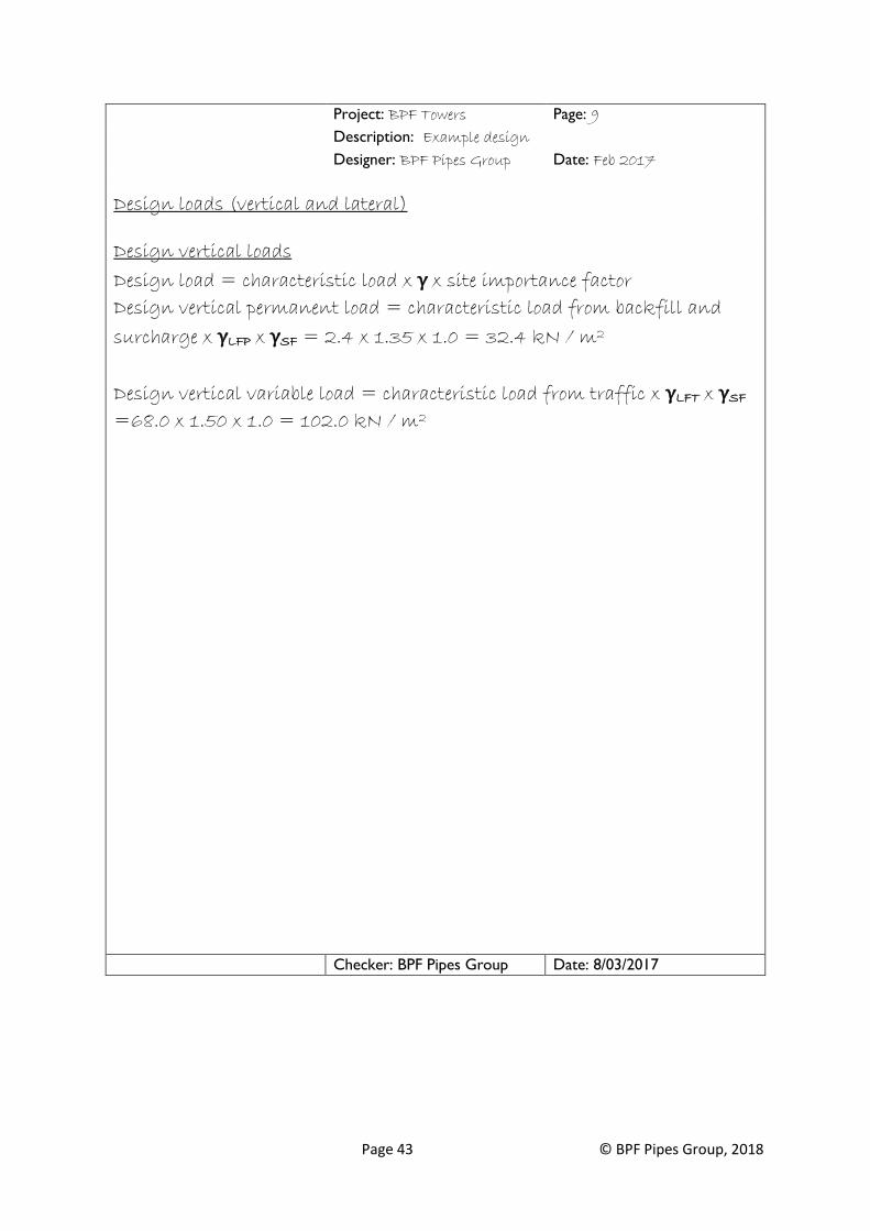
Design loads (vertical and lateral)
Design vertical loads
Design load = characteristic load x γ x site importance factor
Design vertical permanent load = characteristic load from backfill and
surcharge x γLFP x γSF = 2.4 x 1.35 x 1.0 = 32.4 kN / m2
Design vertical variable load = characteristic load from traffic x γLFT x γSF
=68.0 x 1.50 x 1.0 = 102.0 kN / m2
Checker: BPF Pipes Group Date: 8/03/2017
Page 44 © BPF Pipes Group, 2018
8.7 Step 3.7: Design lateral loads (Pages 89 - 93 C737)
The purpose of this step is to derive the design lateral loads using the characteristic loads and partial
factors of safety from the previous calculation sheets.
Design loads = characteristic loads x partial factor of safety x lateral load reduction factor
(LRF).
The calculations for this example are shown on the adjacent page for both permanent and variable
loads.
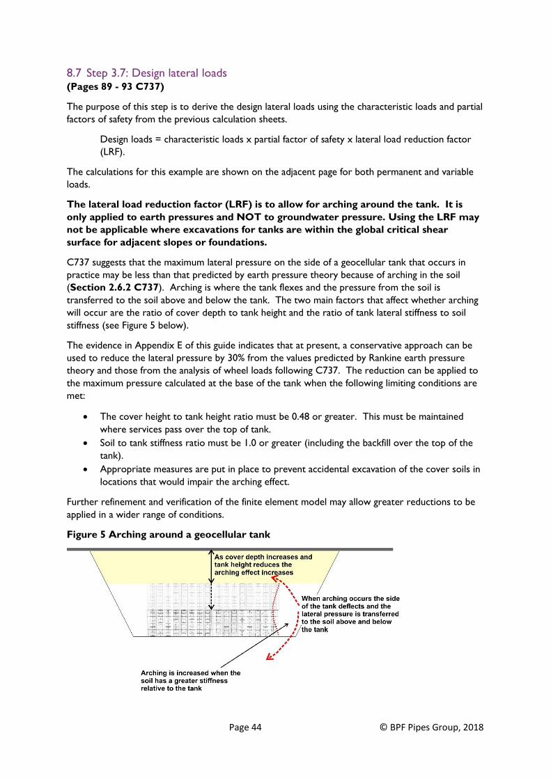
The lateral load reduction factor (LRF) is to allow for arching around the tank. It is
only applied to earth pressures and NOT to groundwater pressure. Using the LRF may
not be applicable where excavations for tanks are within the global critical shear
surface for adjacent slopes or foundations.
C737 suggests that the maximum lateral pressure on the side of a geocellular tank that occurs in
practice may be less than that predicted by earth pressure theory because of arching in the soil
(Section 2.6.2 C737). Arching is where the tank flexes and the pressure from the soil is
transferred to the soil above and below the tank. The two main factors that affect whether arching
will occur are the ratio of cover depth to tank height and the ratio of tank lateral stiffness to soil
stiffness (see Figure 5 below).
The evidence in Appendix E of this guide indicates that at present, a conservative approach can be
used to reduce the lateral pressure by 30% from the values predicted by Rankine earth pressure
theory and those from the analysis of wheel loads following C737. The reduction can be applied to
the maximum pressure calculated at the base of the tank when the following limiting conditions are
met:
• The cover height to tank height ratio must be 0.48 or greater. This must be maintained
where services pass over the top of tank.
• Soil to tank stiffness ratio must be 1.0 or greater (including the backfill over the top of the
tank).
• Appropriate measures are put in place to prevent accidental excavation of the cover soils in
locations that would impair the arching effect.
Further refinement and verification of the finite element model may allow greater reductions to be
applied in a wider range of conditions.
Figure 5 Arching around a geocellular tank

Page 45 © BPF Pipes Group, 2018
Project: BPF Towers Page: 10
Description: Example design
Designer: BPF Pipes Group Date: Feb 2017
Design lateral loads
The tank cover depth is 1.2 m and the tank height is 1.2 m. Therefore, the
cover depth to tank height ratio = 1.0. This is greater than 0.48 and the
reduction factor can be applied.
The failure wedge is in the Class 6N backfill. This will be much stiffer
than the tank and the soil tank stiffness ratio will be greater than 1.0.
Therefore, the reduction factor can be applied.
The lateral earth pressure can be reduced by 30% (i.e., load reduction factor
= 0.7).
Design lateral permanent load
= (characteristic earth pressure x LRF + groundwater) x γLFP x γSF
= (11.23 x 0.7 + 0) x 1.35 x 1.0 = 10.61 kN / m2
Design lateral transient load
= characteristic lateral pressure from traffic x γLFT x γSF x LRF
= 2.08 x 1.5 x 1.0 x 0.7 = 2.18 kN / m2
Checker: BPF Pipes Group Date: 8/03/2017

Page 46 © BPF Pipes Group, 2018
9. Step 4: Determine characteristic strength and apply
partial factors to determine design properties (Pages 76 -78 C737)
9.1 Strength data The characteristic strength and design strength would normally be declared by the supplier of the
tank on the Product Evaluation Form (Page 151 C737). The form for this example is provided in
Table 2, Section 9.5 of this worked example.
The process to be followed by the supplier of the tank to determine the properties is shown in
Figure 4.9 C737. Currently there are no standardised test methods. Work is ongoing to develop
European test standards but this is not likely to cover some of the tests discussed in C737 such as
yield tests and fatigue (cyclic load) tests. More detailed advice on the current test regimes and how
suppliers can provide data for design is provided in Section 12.2 of this guide.
At the time of publication of this guide, most units currently on the market have strength data that is
based on tests that have been completed using the approach described in C680. Therefore, this
example uses the data that is commonly available for most geocellular units. The short-term tests
have been completed using a failure time of 10 minutes. This is an interim process (also used
by current BBA certificates) that should be followed until the information required for
assessing the strength fully in accordance with C737 is published by manufacturers.
Once European or UK Standard test methods are published, these should be adopted
for testing the units.
9.2 Step 4.1: Partial material factors of safety (Pages 77 and 78 C737)
The purpose of this step is to show how a supplier would derive the partial factors of safety to be
applied to the properties of the geocellular units. In the example on the adjacent page, the partial
factor for the long-term creep strength is derived.
The partial factor for the geocellular unit properties is made up of many sub-factors that depend on
the manufacturing process, variability of unit, extrapolation of test data, differences between
laboratory and field performance, global influences (e.g., stacking units) and tolerance to
construction damage.
The factors for this example are given on the adjacent page and are taken from Table 5.2 C737.
For this example:
• The units have creep test lab data with a maximum duration of 5,000 hours.
• Extrapolation of the lab test data from 5,000 hours to 50 years design life would lead to a
higher factor of safety to allow for the uncertainty. However, it is assumed in this example
that the units have a current BBA certificate and have been widely used for over 15 years at
similar cover depths and vehicle loadings to the proposed installation and the supplier has
provided robust evidence that no creep failure or excessive deflection has occurred over
that time. (Note the earliest installation of geocellular tanks in the U.K. was in
the early 1990’s).
• Although not a specific creep test, this information provides further evidence of the creep
performance of the units and reduces the uncertainty in the extrapolation of the creep data
to obtain a long-term strength. Therefore, the designer has used judgement to assess that a
creep test equivalent duration of 10,000 hours can be adopted for deriving the partial factor
of safety to be applied to the long-term strength to allow for uncertainty.

Page 47 © BPF Pipes Group, 2018
• Specific advice on a suitable factor of safety for extrapolation can be obtained from the
manufacturer. It is envisaged that once specific tests standards are in place that longer creep
test durations will remove the need for this approach to be used.
• The design life is 50 years.
In this example, the units are injection moulded units that are manufactured as two pieces. The
units have been in use for over 15 years with no reported failures (caused by inadequate test data).
Therefore, PF3 is assumed to equal 1.0.
The calculated partial factor should not be less than the minimum value of 1.5 quoted in C737.
The partial factor to be applied to the short-term strength in this example is derived in the same
way. All the sub-factors are the same as for the long-term except PF2. For this factor, the same
approach is used but the creep test duration is replaced with the number of load cycles completed
in fatigue tests (or, where appropriate, the equivalent service duration at similar cover depths and
vehicle loading to the proposed installation).

Page 48 © BPF Pipes Group, 2018
BLANK PAGE

Page 49 © BPF Pipes Group, 2018
Project: BPF Towers Page: 11
Description: Example design
Designer: BPF Pipes Group Date: Feb 2017
Partial material factors of safety
Partial factors PF1 to PF5 (Table 5.2 of C737)
Units are factory produced in one moulding, PF1 = 1.0
Extrapolation of creep data
Maximum test duration of WaterBox 1 = 5,000 hours
However, units have been used for over 15 years with no reported failures,
therefore, say creep test date is equivalent to 10,000 hours
PF2 = 1.2r where r = log𝑡𝑑
𝑡𝑚2
td = design life = 50 years = 438,000 hours
tm2 = creep test duration = 10,000 hours
r = log438000
10000 = 1.64 PF2 = 1.21.64 = 1.35
Laboratory and mobilised strength
PF3 = 1.0 (The evidence from the supplier shows that the laboratory test
data is a reasonable indicator of the mobilised strength of the units when
installed. Units have been in use for over 5 years with no known problems,
use 1.0)
Global behaviour
PF4 = 1.0 (The evidence from the supplier shows that there is no unusual
global behaviour. Units have been in use for over 5 years with no known
problems)
Damage during construction PF5 = 1.05
Total material factor γm = PF1 x PF2 x PF3 x PF4 x PF5
γm = 1.0 x 1.35 x 1.0 x 1.0 x 1.05 = 1.42
Minimum value = 1.5 for permanent works
Checker: BPF Pipes Group Date: 8/03/2017

Page 50 © BPF Pipes Group, 2018
9.3 Step 4.2: Design strengths The purpose of this step is to derive the design strength (short-term and long-term).
The characteristic strength is divided by the appropriate partial factor as shown on the adjacent
page.

Page 51 © BPF Pipes Group, 2018
Project: BPF Towers Page: 12
Description: Example design
Designer: BPF Pipes Group Date: Feb 2017
Design strength
Design strength = 𝐶ℎ𝑎𝑟𝑎𝑐𝑡𝑒𝑟𝑖𝑠𝑡𝑖𝑐 𝑠𝑡𝑟𝑒𝑛𝑔𝑡ℎ
𝑀𝑎𝑡𝑒𝑟𝑖𝑎𝑙 𝑝𝑎𝑟𝑡𝑖𝑎𝑙 𝑓𝑎𝑐𝑡𝑜𝑟 𝛾𝑚
Characteristic short- and long-term strength in the vertical and lateral
direction for the WaterBox 1 are declared by the supplier on the Product
Evaluation Form (Table 2 in Section 9.5 of this worked example).
Design vertical short-term strength, PDS = 𝑷𝑪𝑲𝑺
𝛄𝒎𝒔 =
𝟐𝟗𝟎
𝟏.𝟓 = 193.3 kN / m2
Design vertical long-term strength, PDL = 𝑷𝑪𝑲𝑳
𝛄𝒎𝒔 =
𝟏𝟐𝟒
𝟏.𝟓 = 82.7 kN / m2
Design lateral short-term strength, PDSL = 𝑷𝑪𝑲𝑺𝑳
𝛄𝒎𝒔 =
𝟔𝟒
𝟏.𝟓 = 42.7 kN / m2
Design lateral long-term strength, PDLL = 𝑷𝑪𝑲𝑳𝑳
𝛄𝒎𝒔 =
𝟐𝟕
𝟏.𝟓 = 18.0 kN / m2
Checker: BPF Pipes Group Date: 8/03/2017

Page 52 © BPF Pipes Group, 2018
9.4 Step 4.3: Product Evaluation Form (Page 151 C737)
In this worked example, the geocellular units to be used are manufactured by Mr Plastic
Manufacturing Company Limited. WaterBox 1 units will be supplied. Data supplied by the company
on the Product Evaluation Form is shown on the adjacent page.
Testing and confirmation checklist – this part of the form shows the data that has been
supplied by Mr Plastic Manufacturing Company Limited, given in Table 2 of this guide for this worked
example. Note that professional indemnity insurance (PI) is not required for this example as Mr
Plastic Manufacturing Company Limited is not contractually employed to provide design services. For
schemes where the manufacturer/supplier is employed to provide the design, then PI is likely to be
required. This information is required to allow the approach described in this guide to be used for
design.
The porosity of the units in this example is 95%. Porosity is used in storage volume calculations.
This value is placed in the box on the form labelled “Void Ratio”. Note that void ratio is different to
porosity (SuDS Manual 2015, Page 659).
Porosity = volume of voids/total volume of material.
Voids ratio = porosity/(1 – porosity).
In the example Product Evaluation Form, the unit strength parameters are defined as follows:
• The ultimate strength is the mean value of the short-term strength derived using the
laboratory test methods that are described in C680 and are used by BBA for most current
certificates.
• Characteristic strength is the creep strength for the design life of the project – in this
example 50 years.
• Design strength is the factored characteristic strength for the design life of the project – in
this example 50 years.
• Reference strength is the creep strength for a design life of 20 years. The form in C737
incorrectly indicates that this is 50 years (to the right of the boxes) but the text in the main
body of C737 makes it clear it should be 20 years.
The characteristic long-term or creep strength in this example has been derived by assuming the
coefficient of variation for the short-term tests is the same as that for the creep tests. This has been
shown by test data to be a reasonable approach. The adoption of an additional factor of safety of 2
that is applied to the COV2 for long-term strength in C737 (Page 62) is not required.
In this example, a partial factor for the material properties is 1.5 as calculated in the preceding pages
of this guide.
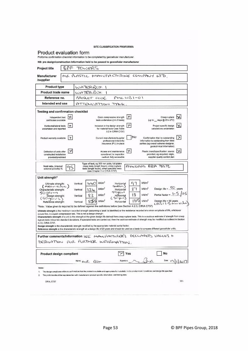
Page 53 © BPF Pipes Group, 2018

Page 54 © BPF Pipes Group, 2018
9.5 Step 4.4: Additional data to be appended to Product Evaluation Form In addition to the data on the Product Evaluation Form, in this example the yield strength of the units
is required. For this example, it is assumed that there is no yield test data and the yield strength is
taken as 70% of the short-term ultimate strength. This is a characteristic value of short-term
ultimate strength, derived using the mean strength and standard deviation, as described on Page 62
C737.
The evidence from cyclic loading tests on various polypropylene geocellular tanks indicates that
fatigue from low level and relatively infrequent cyclic loads does not cause premature failure (for
example, from daily traffic by a few HGVs). This is because polypropylene is resistant to fatigue
failure and testing on units has shown that it is not an issue at stresses up to 40% of the short-term
strength and application of 21,000 load cycles. There is currently no standard method of cyclic or
fatigue load testing. If units are to be subject to very frequent cyclic loading, for example, under a
road designed to carry tens or hundreds of HGVs per day or in a rail environment (i.e., a Traffic
Zone E2 and E3 - Class 3 design), then cyclic load tests that replicate the service conditions should
be carried out.
For some units, testing with a 300 mm diameter plate gives a lower strength than with a full plate. If
the strength parameters are derived from full plate tests, the supplier should confirm that these give
the lowest strength.
The deflection of the units under short-term loads (elastic deflection) and during creep should be
stated.
The creep coefficient is defined on Page 169 of C737 and is taken from the straight-line portion of
the deflection vs time graph for an appropriate test load that slightly exceeds the design load. In
Table 2, the vertical creep coefficient is provided by the unit supplier for four different test loads
that cover an equivalent soil cover depth from 1 m to 2.5 m (assuming a soil unit weight of
20 kN/m3). The lateral creep coefficient is also provided at four test loads that cover an equivalent
depth from 1.5 m to 3 m (assuming an active earth pressure coefficient of 0.33 and soil unit weight
of 20 kN/m3).
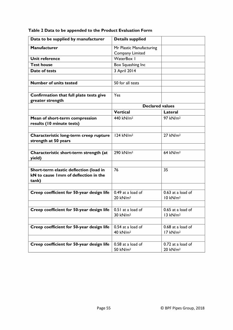
Page 55 © BPF Pipes Group, 2018
Table 2 Data to be appended to the Product Evaluation Form
Data to be supplied by manufacturer Details supplied
Manufacturer Mr Plastic Manufacturing
Company Limited
Unit reference WaterBox 1
Test house Box Squashing Inc
Date of tests 3 April 2014
Number of units tested 50 for all tests
Confirmation that full plate tests give
greater strength
Yes
Declared values
Vertical Lateral
Mean of short-term compression
results (10 minute tests)
440 kN/m2 97 kN/m2
Characteristic long-term creep rupture
strength at 50 years
124 kN/m2 27 kN/m2
Characteristic short-term strength (at
yield)
290 kN/m2 64 kN/m2
Short-term elastic deflection (load in
kN to cause 1mm of deflection in the
tank)
76 35
Creep coefficient for 50-year design life 0.49 at a load of
20 kN/m2
0.63 at a load of
10 kN/m2
Creep coefficient for 50-year design life 0.51 at a load of
30 kN/m2
0.65 at a load of
13 kN/m2
Creep coefficient for 50-year design life 0.54 at a load of
40 kN/m2
0.68 at a load of
17 kN/m2
Creep coefficient for 50-year design life 0.58 at a load of
50 kN/m2
0.72 at a load of
20 kN/m2
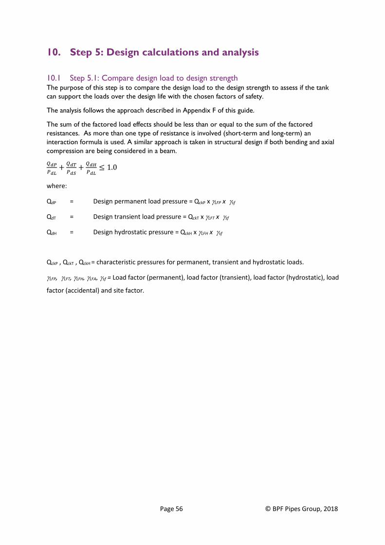
Page 56 © BPF Pipes Group, 2018
10. Step 5: Design calculations and analysis
10.1 Step 5.1: Compare design load to design strength The purpose of this step is to compare the design load to the design strength to assess if the tank
can support the loads over the design life with the chosen factors of safety.
The analysis follows the approach described in Appendix F of this guide.
The sum of the factored load effects should be less than or equal to the sum of the factored
resistances. As more than one type of resistance is involved (short-term and long-term) an
interaction formula is used. A similar approach is taken in structural design if both bending and axial
compression are being considered in a beam.
𝑄𝑑𝑃
𝑃𝑑𝐿+
𝑄𝑑𝑇
𝑃𝑑𝑆+
𝑄𝑑𝐻
𝑃𝑑𝐿≤ 1.0
where:
QdP = Design permanent load pressure = QckP x LFP x sf
QdT = Design transient load pressure = QckT x LFT x sf
QdH = Design hydrostatic pressure = QckH x LFH x sf
QckP , QckT , QckH = characteristic pressures for permanent, transient and hydrostatic loads.
LFP, LFT, LFHLFAsf = Load factor (permanent), load factor (transient), load factor (hydrostatic), load
factor (accidental) and site factor.

Page 57 © BPF Pipes Group, 2018
Project: BPF Towers Page: 13
Description: Example design
Designer: BPF Pipes Group Date: Feb 2017
Design analysis
Design loads and strengths taken from previous calculation sheets. Loads
Section 8.6, Calculation sheet Page 9, Section 8.7, Calculation sheet Page
10 and Strengths Section 9.3, Calculation sheet Page 12.
Design equation
𝐷𝑒𝑠𝑖𝑔𝑛 𝑝𝑒𝑟𝑚𝑎𝑛𝑒𝑛𝑡 𝑙𝑜𝑎𝑑
𝐷𝑒𝑠𝑖𝑔𝑛 𝑙𝑜𝑛𝑔 𝑡𝑒𝑟𝑚 𝑠𝑡𝑟𝑒𝑛𝑔𝑡ℎ+
𝐷𝑒𝑠𝑖𝑔𝑛 𝑠ℎ𝑜𝑟𝑡 𝑡𝑒𝑟𝑚 𝑙𝑜𝑎𝑑
𝐷𝑒𝑠𝑖𝑔𝑛 𝑠ℎ𝑜𝑟𝑡 𝑡𝑒𝑟𝑚 𝑠𝑡𝑟𝑒𝑛𝑔𝑡ℎ < 1.0
In this example, the hydrostatic load is assumed to be zero in the vertical
direction and is included in the permanent load in the lateral direction.
Vertical
32.40
82.70+
102.0
193.3= 0.92
Less than 1.o, so OK
Lateral
10.61
18.0+
2.18
42.7= 0.64
Less than 1.o, so OK
Checker: BPF Pipes Group Date: 8/03/2017

Page 58 © BPF Pipes Group, 2018
Blank page

Page 59 © BPF Pipes Group, 2018
10.2 Step 5.2: Compare predicted tank deformation to acceptable limits for the site The purpose of this step is to estimate the likely deflections under short-term and long-term loads.
Example calculations are also provided on Pages 167 - 171 C737.
The calculations in C737 suggest that elastic deformation under wheel loads is built out during
construction. This is not the case because although the initial elastic part of a creep curve is built
out during construction when the permanent backfill is placed, if an additional wheel load is applied
to the backfilled tank, further elastic deflection will occur. This is normally fully recoverable on
unloading. If transient loads are left for a period, some creep will occur but a significant proportion
of this will be recoverable as well. This is shown in Figure 6. Experience has shown that if tanks are
designed following this example, then the influence of cars being parked over the top of tanks for up
to 8 hours per day should be negligible.
Figure 6 Deflection at ground surface during and after construction
This example assesses the influence of short-term wheel loads on deflection once the tank is
installed.
The characteristic loads are the same as those derived earlier in these calculations.
Deflection is a serviceability limit state and appropriate partial factors of safety are used to
determine the design loads. In this example, the load factors from Table 5.9 of C737 are all equal
to 1.0.

Page 60 © BPF Pipes Group, 2018
Creep over time under backfill
In this example, it is assumed that the short-term and long-term construction deflections will occur
over a 12-month period as the tank is backfilled to the underside of the asphalt level after backfilling
the tank and the asphalt pavement layers are constructed later towards the end of the project.
The creep coefficient taken from the supplier’s data is 0.51 vertically (for a load of 30 kN/m2 which is
higher than the design permanent load of 24 kN/m2). The creep coefficient is 0.63 laterally (which is
for a load of 10 kN/m2, higher than the design permanent load of 7.84 kN/m2). In both cases, this
will result in a slight over-estimation of the estimated deflection.
Allowable creep deformations of 10 mm laterally and 5 mm vertically should not cause problems to
most road or car park surfaces. Greater allowable limits may be acceptable if agreed with the client
and an assessment of the serviceability of the tank and overlying construction is made.

Page 61 © BPF Pipes Group, 2018
Project: BPF Towers Page: 14
Description: Example design
Designer: BPF Pipes Group Date: Feb 2017
Deflection
Characteristic loads from previous sheets:
Vertical variable = 68 kN/m2 (overlap of wheel zones)
Vertical variable = 37 kN/m2 (no overlap)
Vertical permanent load = 24 kN/m2
Lateral permanent load = 11.2 kN/m2
Partial factor of safety for serviceability limit state = 1.0 (for all load
cases)
Therefore, Design loads = Characteristic loads x 1.0
Vertical creep deflection
Applied permanent load = 24 kN/m2
Therefore, use creep coefficient from test at 30 kN/m2 = 0.51
Creep at 12 months (8760 hours) = 0.51Ln(8760) = 4.6 mm
Creep at 50 years (438,000 hours) = 0.51Ln(438,000) = 6.6 mm
Creep after pavement construction = 6.6 – 4.6 = 2 mm (this is acceptable)
Lateral creep deflection
Applied permanent load = 11.2 kN/m2
Therefore, use creep coefficient from test at 13 kN/m2 = 0.65
Creep at 50 years (438,000 hours) = 0.65Ln(438,000) = 8.5 mm
This is less than 10mm and is acceptable
Checker: BPF Pipes Group Date: 8/03/2017

Page 62 © BPF Pipes Group, 2018
Short-term vertical deflection from wheels
This calculation follows the approach described on Page 170 of C737.
It is assumed that short-term vertical deflections due to the weight of backfill are built out.
The worst-case situation for tank deflection and its impact on the surfacing materials will be at the
edge of the tank. Soil is normally a lot stiffer than the tanks and the differential movement will be at
a maximum at this location (Figure 7). Differential movement is assumed to occur over the width of
the wheel overlap.
Figure 7 Tank deflection relative to surrounding area
The allowable maximum vertical movement of a concrete block pavement surface under a wheel
load is 1.5 mm in this example. This is a value that has been widely used for tanks that are covered
by concrete block paving and that are only subject to occasional traffic by the maximum design load.
Other limiting values could be used in agreement with the pavement design engineer and/or client.
The more sensitive the surfacing material is to movement or the more frequent the deflection
occurs the lower the allowable value is likely to be.
These examples ignore any deflection in the soil materials above and below the tank. Normally this
is negligible compared to deflection of the tank. There is no need to consider this in routine designs.
Therefore, the analysis uses a limiting deflection in the tank of 1.5 mm.
The elastic short-term deflection is taken from the supplier’s data and, in this case, is 1 mm per
76 kN/m2 applied load.
The allowable differential deflection (curvature) for a car park is 1 in 100 to 1 in 200 (Page 170
C737).
In this example, testing for the units has shown that under concentrated loads such as wheel loads,
the deflection that occurs in the top of one layer of units does not increase if there is more than one
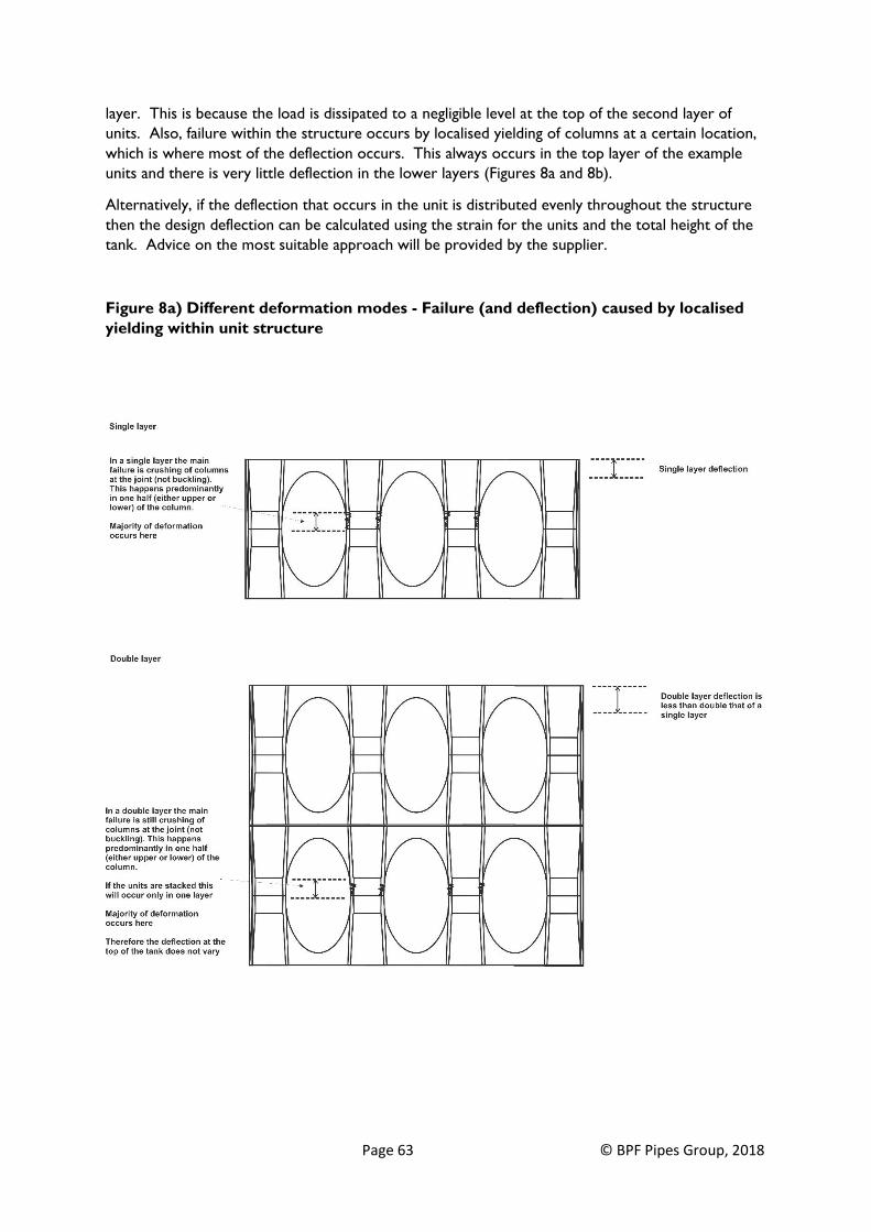
Page 63 © BPF Pipes Group, 2018
layer. This is because the load is dissipated to a negligible level at the top of the second layer of
units. Also, failure within the structure occurs by localised yielding of columns at a certain location,
which is where most of the deflection occurs. This always occurs in the top layer of the example
units and there is very little deflection in the lower layers (Figures 8a and 8b).
Alternatively, if the deflection that occurs in the unit is distributed evenly throughout the structure
then the design deflection can be calculated using the strain for the units and the total height of the
tank. Advice on the most suitable approach will be provided by the supplier.
Figure 8a) Different deformation modes - Failure (and deflection) caused by localised
yielding within unit structure
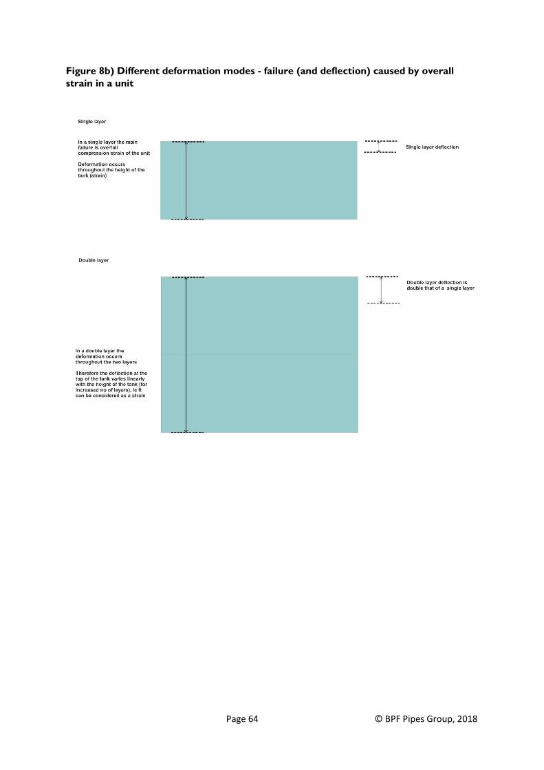
Page 64 © BPF Pipes Group, 2018
Figure 8b) Different deformation modes - failure (and deflection) caused by overall
strain in a unit
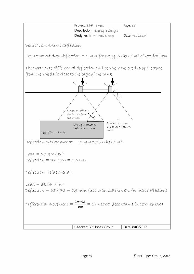
Page 65 © BPF Pipes Group, 2018
Project: BPF Towers Page: 15
Description: Example design
Designer: BPF Pipes Group Date: Feb 2017
Vertical short-term deflection
From product data deflection = 1 mm for every 76 kN / m2 of applied load.
The worst case differential deflection will be where the overlap of the zone
from the wheels is close to the edge of the tank.
Deflection outside overlap → 1 mm per 76 kN / m2
Load = 37 kN / m2
Deflection = 37 / 76 = 0.5 mm
Deflection inside overlap
Load = 68 kN / m2
Deflection = 68 / 76 = 0.9 mm (less than 1.5 mm OL for max deflection)
Differential movement = 0.9−0.5
400 = 1 in 1000 (less than 1 in 200, so OK)
Checker: BPF Pipes Group Date: 8/03/2017

Page 66 © BPF Pipes Group, 2018
10.3 Step 5a: Global deformation and site stability assessment (Pages 100 and 101 C737)
The purpose of this step is to assess any global (or overall) stability issues as described on Pages
100 and 101 C737.
Global deformation and site stability checks are not required routinely and are only completed if
there are site-specific concerns.
Interaction checks such as assessing nearby slopes, building foundations, etc. (5.3.5.2 C737) are not
required routinely and are only completed if there are site-specific concerns.
In this example, where the site is flat and the tanks are outside the zone of influence of any
structures, there is no requirement for a global stability check. If global stability is to be checked, it
is likely to require input from a specialist geotechnical engineer.
Assessment of uplift or flotation (Page 95 C737) is not included in this example because the tank is
above the water table. Uplift does need to be considered if the tank is likely to be below the
groundwater at any time (seasonal variation in levels need to be considered). It is also required
where a tank is constructed in clay soils and the water level in the backfilled excavation could rise
over time. In online tanks, any water that does infiltrate the backfill can usually seep away along
bedding and surround of outlet pipes.

Page 67 © BPF Pipes Group, 2018
11. Step 6: Prepare geotechnical design report (Page 114 C737)
The purpose of the geotechnical design report is to summarise the critical assumptions and
parameters used in the design calculations. This is a requirement of Eurocode 7.
The purpose of the report is to make those building the tank aware of the critical design factors and
assumptions made. The most effective form of communication is a short one- or two-page summary
of the information (including a diagrammatic ground conceptual model).
Any communication of relevant unusual risk that is required under the CDM Regulations should also
be included here as well as on the design drawings.
The geotechnical design report for this worked example is provided on the following two pages.

Page 68 © BPF Pipes Group, 2018
Table 3 Example geotechnical design report
Project Title: BPF Towers Job No: DC01023
Tank Reference: Attenuation 1 Made by: SAW
Site Classification: 1 Checked by: SM
Relevant Reports with Factual and
Interpretative Information:
Dr Dirt Limited, Site investigation report for
BPF Towers. V2 September 2016
Critical Assumptions in Calculations
Regarding Ground Conditions
Stratigraphy – see CGM below
Parameters – See CGM below
Excavation batter at 45°
0.5 m working space around tank at base (flat
area)
100 mm of sand over top of tank
General granular fill over top of tank
Class 6N around sides compacted using light
plate compactor (maximum force per blow
15 kN)
Relevant Codes and Standards:
Eurocode EC 7
BS 5930
Type of Units and Manufacture
Mr Plastic Manufacturing Company Limited
WaterBox 1
Refer to manufacturer’s installation guidelines
Description of Relevant Aspects of Site
and Surroundings:
Tank is located outside zone of influence of
buildings or embankments
It is assumed that the site is level.
Information to be Verified During
Construction
Ground profile in side of excavation
Glacial till is present as firm to stiff clay in base
of excavation
value of Class 6N
Excavation batter is at 45° with 0.5 m working
space
Verification of geomembrane wrap to tank in
accordance with CIRIA C735
Critical Assumptions in Calculations
Regarding Loads
Load Class = C
Type of vehicles = cars and accidental passage
of HGVs
Construction traffic = construction traffic only
allowed after completion of pavement to final
level. Tank must be fenced off prior to this
No cranes or similar
Maintenance and Monitoring
Requirements
No regular requirements for
structural/geotechnical purposes
See drainage design for specific requirements
relating to hydraulic performance and silt
removal

Page 69 © BPF Pipes Group, 2018
Table 3 Example geotechnical design report (continued)
Conceptual ground model (CGM) assumed in the design
Ground properties – those highlighted in blue to be checked on site during excavation
and installation
Stratum Typical
thickness
assumed in
design
Unit weight
assumed in
design
Effective angle of
friction assumed in
design
Made Ground (medium dense black sandy GRAVEL
of ash and clinker)
1.0 m 18 kN/m3 32o
Glacial Till (firm to stiff dark grey silty sandy CLAY
with much fine to coarse gravel)
6.0 m 20 kN/m3 28o
Coal Measures (not investigated). Geological map
indicates series of mudstone, siltstone, sandstone
and coal seams. No workings.
100 m+ n/a n/a
Class 6N backfill to Specification for Highway Works -- 18 kN/m3 36o
Class 1 General granular fill to Specification for
Highway Works
-- 18 kN/m3 32o

Page 70 © BPF Pipes Group, 2018
12. Additional information
12.1 Existing tanks The BPF Pipes Group has published a position statement with respect to the use of C737 and C680
https://bpfpipesgroup.com/support-downloads/position-statements/.
12.2 Testing The short- and long-term compression tests on geocellular units are not like tests on small samples
of materials (for example, tensile tests on strips of plastic material or compression tests on solid
cubes of concrete). An individual geocellular unit is a complex structure, not a solid, and
compression tests are used to obtain an indication of its performance in service. The use of the test
results allows a simplified design method to be used. The alternative would be to carry out a
complex structural analysis of the units for every site, which is prohibitively time consuming and not
practical.
There are currently no published standard test methods available, although work is in progress to
develop these. Most units available in the UK market have been tested following the methods
described in C680 or very similar approaches that are relatively consistent between manufacturers.
Experience has shown that providing the overall principles described in the methods described in
C680 are followed, the practical impact on the quoted strengths is limited. It is important to
remember that this is a practical engineering exercise and not a detailed scientific investigation. The
levels of accuracy in the test method should reflect that. Once European or UK Standard test
methods are published these should be adopted for testing the units.
Most units on the market have strength data that is based on tests completed using the basic
approach described in C680. The short-term tests have been completed using a failure time of 10
minutes. Extending the failure time for short-term tests as suggested in C737 is not considered
necessary. Tests on other plastic materials such as geogrids determine the short-term strength
using much quicker loading rates.
Where suppliers have completed the more specialist tests described in C737, these results can be
used. If such tests are not available, the strength parameters can be derived (conservatively) using
the alternative approaches that are explained in this guide.
There are practical issues at present with completing some of the new tests listed in C737 as well as
availability of laboratory time across Europe. One issue is determining the fatigue strength by cyclic
load testing. Issues that need to be resolved before a standard test method can be published include
determining an acceptable level of control over the loading cycles (the load varies quite significantly
with each cycle unless very expensive control machinery and jacks are used) and the test duration.
Many suppliers have creep and creep rupture tests that have been completed using 300 mm
diameter plates because of practical and safety issues when using full plates on units with a large
surface area on the top or side faces. This data is valid if the correlation between the short-term
strength derived from full plate and that from 300 mm plates is known. The correlation can be used
to adjust 300 mm plate creep results to full plate values. Experience has shown that this is a valid
approach and that the variability shown in short-term tests with various plates is reflected in creep
and creep rupture tests.
Long-term creep test duration depends on the required design life. It can be a minimum of
2,000 hours (Page 60 C737). The longer the test duration the lower the partial factor and the
higher the design life. The creep time is divided by 100 to give the design life (in years) as follows:
10,000 hours required for a design life of 100 years.

Page 71 © BPF Pipes Group, 2018
5,000 hours required for a design life of 50 years.
2,000 hours required for a design life of 20 years.
If a full suite of creep and creep rupture test data is not available, the creep strength can be
determined using reduction factors applied to the short-term strength. This approach is used in
Australian Standard AS 4678–2002, Earth-Retaining Structures. Creep reduction factors for different
materials are given in that standard (Table K3). For polypropylene, the reduction factors are 0.2 for
a 30-year design life and 0.17 for a 100-year design life.
The yield strength can be defined using the test approach in C737 with loading and unloading (a
standard test method needs to be developed) or the following alternatives can be adopted:
• Assume that the yield strength is 70% of the peak failure strength from short-term tests
(assumed in this worked example).
• Using the short-term test data, consider the intersection point of the elastic zone from the
stress/deflection curve with that of the plastic zone (see Appendix G of this guide). This is
the approach adopted in many current BBA certificates.
The yield strength is the point after which the material begins to deform plastically whereas the
ultimate or peak strength is the maximum load that the unit can withstand. This is shown in Figure
9.
Figure 9 Determination of yield strength from short-term compression tests
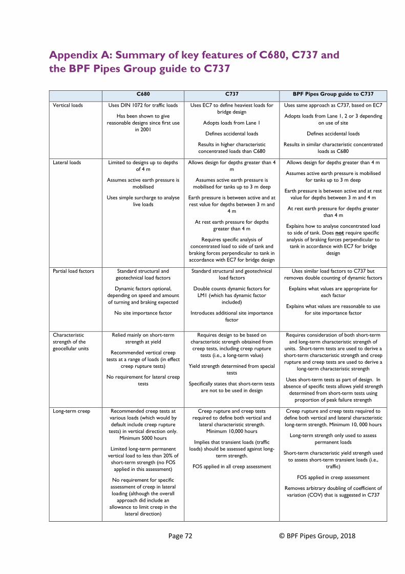
Page 72 © BPF Pipes Group, 2018
Appendix A: Summary of key features of C680, C737 and
the BPF Pipes Group guide to C737
C680 C737 BPF Pipes Group guide to C737
Vertical loads Uses DIN 1072 for traffic loads
Has been shown to give
reasonable designs since first use
in 2001
Uses EC7 to define heaviest loads for
bridge design
Adopts loads from Lane 1
Defines accidental loads
Results in higher characteristic
concentrated loads than C680
Uses same approach as C737, based on EC7
Adopts loads from Lane 1, 2 or 3 depending
on use of site
Defines accidental loads
Results in similar characteristic concentrated
loads as C680
Lateral loads Limited to designs up to depths
of 4 m
Assumes active earth pressure is
mobilised
Uses simple surcharge to analyse
live loads
Allows design for depths greater than 4
m
Assumes active earth pressure is
mobilised for tanks up to 3 m deep
Earth pressure is between active and at
rest value for depths between 3 m and
4 m
At rest earth pressure for depths
greater than 4 m
Requires specific analysis of
concentrated load to side of tank and
braking forces perpendicular to tank in
accordance with EC7 for bridge design
Allows design for depths greater than 4 m
Assumes active earth pressure is mobilised
for tanks up to 3 m deep
Earth pressure is between active and at rest
value for depths between 3 m and 4 m
At rest earth pressure for depths greater
than 4 m
Explains how to analyse concentrated load
to side of tank. Does not require specific
analysis of braking forces perpendicular to
tank in accordance with EC7 for bridge
design
Partial load factors Standard structural and
geotechnical load factors
Dynamic factors optional,
depending on speed and amount
of turning and braking expected
No site importance factor
Standard structural and geotechnical
load factors
Double counts dynamic factors for
LM1 (which has dynamic factor
included)
Introduces additional site importance
factor
Uses similar load factors to C737 but
removes double counting of dynamic factors
Explains what values are appropriate for
each factor
Explains what values are reasonable to use
for site importance factor
Characteristic
strength of the
geocellular units
Relied mainly on short-term
strength at yield
Recommended vertical creep
tests at a range of loads (in effect
creep rupture tests)
No requirement for lateral creep
tests
Requires design to be based on
characteristic strength obtained from
creep tests, including creep rupture
tests (i.e., a long-term value)
Yield strength determined from special
tests
Specifically states that short-term tests
are not to be used in design
Requires consideration of both short-term
and long-term characteristic strength of
units. Short-term tests are used to derive a
short-term characteristic strength and creep
rupture and creep tests are used to derive a
long-term characteristic strength
Uses short-term tests as part of design. In
absence of specific tests allows yield strength
determined from short-term tests using
proportion of peak failure strength
Long-term creep Recommended creep tests at
various loads (which would by
default include creep rupture
tests) in vertical direction only.
Minimum 5000 hours
Limited long-term permanent
vertical load to less than 20% of
short-term strength (no FOS
applied in this assessment)
No requirement for specific
assessment of creep in lateral
loading (although the overall
approach did include an
allowance to limit creep in the
lateral direction)
Creep rupture and creep tests
required to define both vertical and
lateral characteristic strength.
Minimum 10,000 hours
Implies that transient loads (traffic
loads) should be assessed against long-
term strength.
FOS applied in all creep assessment
Creep rupture and creep tests required to
define both vertical and lateral characteristic
long-term strength. Minimum 10, 000 hours
Long-term strength only used to assess
permanent loads
Short-term characteristic yield strength used
to assess short-term transient loads (i.e.,
traffic)
FOS applied in creep assessment
Removes arbitrary doubling of coefficient of
variation (COV) that is suggested in C737

Page 73 © BPF Pipes Group, 2018
C680 C737 BPF Pipes Group guide to C737
Partial material
factors
Short-term – 2.75
Long-term – 1.0 to 1.5
Long-term – varies depending on
several factors from 1.5 to 2.7 for
permanent works. Can be excessive if
applied without thought
Short-term – N/A
Long-term – varies depending on several
factors from 1.5 to 2.7 but gives advice on
reasonable values
Short-term – varies depending on several
factors from 1.5 to 2.7 but gives advice on
reasonable values
Analysis Vertical and lateral short-term
and long-term loads considered
against factored short-term
strengths
Long-term vertical loads
compared to long-term strength
Analysis of elastic settlement
under traffic loads
Short and long term vertical and lateral
loads compared to long term strength
Overly theoretical discussion of
settlement for buildings and no clear
advice on assessment for geocellular
tanks
Long-term vertical and lateral loads
compared to long-term strength
Short-term vertical and lateral loads
compared to yield strength
Interaction formula used to balance short-
and long-term assessment
Simplified assessment of short-term and
long-term settlement with clear advice on
analysis of geocellular tanks (based on
approach that has been proven to work in
practice for most types of tank)
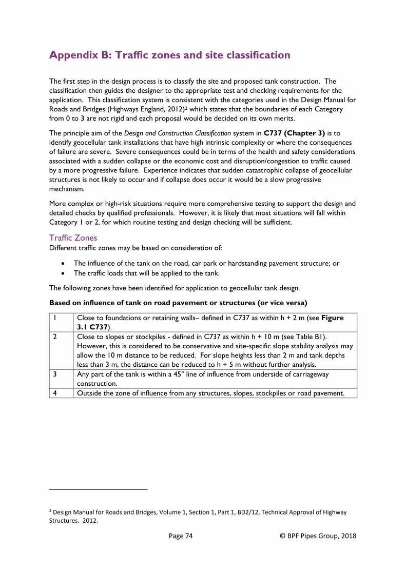
Page 74 © BPF Pipes Group, 2018
Appendix B: Traffic zones and site classification
The first step in the design process is to classify the site and proposed tank construction. The
classification then guides the designer to the appropriate test and checking requirements for the
application. This classification system is consistent with the categories used in the Design Manual for
Roads and Bridges (Highways England, 2012)2 which states that the boundaries of each Category
from 0 to 3 are not rigid and each proposal would be decided on its own merits.
The principle aim of the Design and Construction Classification system in C737 (Chapter 3) is to
identify geocellular tank installations that have high intrinsic complexity or where the consequences
of failure are severe. Severe consequences could be in terms of the health and safety considerations
associated with a sudden collapse or the economic cost and disruption/congestion to traffic caused
by a more progressive failure. Experience indicates that sudden catastrophic collapse of geocellular
structures is not likely to occur and if collapse does occur it would be a slow progressive
mechanism.
More complex or high-risk situations require more comprehensive testing to support the design and
detailed checks by qualified professionals. However, it is likely that most situations will fall within
Category 1 or 2, for which routine testing and design checking will be sufficient.
Traffic Zones Different traffic zones may be based on consideration of:
• The influence of the tank on the road, car park or hardstanding pavement structure; or
• The traffic loads that will be applied to the tank.
The following zones have been identified for application to geocellular tank design.
Based on influence of tank on road pavement or structures (or vice versa)
1 Close to foundations or retaining walls– defined in C737 as within h + 2 m (see Figure
3.1 C737).
2 Close to slopes or stockpiles - defined in C737 as within h + 10 m (see Table B1).
However, this is considered to be conservative and site-specific slope stability analysis may
allow the 10 m distance to be reduced. For slope heights less than 2 m and tank depths
less than 3 m, the distance can be reduced to h + 5 m without further analysis.
3 Any part of the tank is within a 45° line of influence from underside of carriageway
construction.
4 Outside the zone of influence from any structures, slopes, stockpiles or road pavement.
2 Design Manual for Roads and Bridges, Volume 1, Section 1, Part 1, BD2/12, Technical Approval of Highway Structures. 2012.

Page 75 © BPF Pipes Group, 2018
Based on traffic load
A Anywhere that vehicle access is not possible (e.g., due to fences or barriers, road layout
or topography).
B Anywhere that only cars can access due to physical constraints.
C Anywhere that HGVs will only access as an “accidental load” (i.e., not regular HGV traffic,
for example, vehicle overrun on a verge at the back of a footway).
D Anywhere that is subject to limited HGV traffic at very low speed (<15 mph) such as fire
tenders and refuse trucks.
E Everywhere else (assumed to be subject to regular unrestricted HGV traffic). This
category is split into three sub-categories depending on the type of HGV loading that is
expected (E1 to E3). E1 is for areas where HGVs will be regular and moving at low
speeds such as lorry parks and loading bays. E2 would cover some estate roads in
residential developments and E3 would cover trunk roads and motorways. In the latter
case, in the running lanes of motorways (including the occasional hard shoulder on Smart
Motorways), specific assessment of the special vehicle loads should be undertaken to the
requirements of Highways England.
The zone for a tank will be a combination of the position in relation to zones of influence (1 to 4)
and the likely traffic load (A to E). For example, a tank that is outside the zone of influence of any
structures or roads and is not accessible to vehicles would be defined as Zone 4A.
Examples of traffic zones Examples of situations that are typical of each of the traffic zones A to E are shown in Table B.1.
There is no consideration of the zone of influence in the Table (i.e., all situations are considered to
be Zone 4).

Page 76 © BPF Pipes Group, 2018
Table B.1 Example traffic zones
Zone Description Examples
A Anywhere that vehicle access
is not possible (e.g., due to
fences or barriers).
Triangular area between Motorway and slip road is not accessible
to vehicles.
Wide central reservation on approach to a bridge is not accessible
to vehicles due to barriers.
Grassed area in a roundabout under flyover is not accessible to
vehicles due to bank and shrub/bush vegetation.
B Anywhere that only cars can
access due to physical
constraints, e.g., width or
height barriers.
Car park with a height restriction barrier.
C Anywhere that HGVs will only
access as an “accidental load”
(i.e., not regular HGV traffic,
for example, vehicle overrun
on a verge at the back of a
footway).
A wide verge behind a footway
The grassed area of a roundabout is not readily accessible to HGV
traffic due to earth mounds.
D Anywhere that is subject to
limited HGV traffic at low
speed such as roads with
access for fire tenders and
refuse trucks.
An example for a minor access road in a residential development is
given in Kent Design Guide. Section 2 Creating the Design. Step 3
Designing for Movement3.
E Everywhere else (assumed to
be subject to regular
unrestricted HGV traffic).
An example for a local distributor road in a residential
development is given in Kent Design Guide. Section 2 Creating the
Design. Step 3 Designing for Movement.
3 https://www.kent.gov.uk/__data/assets/pdf_file/0018/12096/design-guide-movement.pdf

Page 77 © BPF Pipes Group, 2018
Site classification for the traffic zones Each of the preceding zones has been classified in accordance with the site classification system
described in C737. Some adaptations have been made based on experience of using the system.
The need to adapt the system is recognised in C737 which states:
“The system will require further testing in use to allow modifications and developments to be made, as it is
inevitable that not all circumstances will have been foreseen and a process of evolution is likely”.
A summary of the classification of the different traffic zones using the C737 methodology, together
with the required design checks and testing, is provided in Table B.2. This is limited to locations
outside the zone of influence to structures, slopes or road pavements.

Page 78 © BPF Pipes Group, 2018
Table B.2 Classification, design checks and testing requirements – based on traffic zones (outside any zone of influence to structures,
etc.)
Traffic
zone
General
description
Type of site
Sco
re
Use
Sco
re
Information
Sco
re
Topography
Sco
re
Location
Sco
re
Depth
to base
Sco
re
Cover (see
note at
base of
table)
Sco
re
Construction
phase
Sco
re
Classification Testing
requirements
Recommended
actions/roles
(Table 3.2 C737)
Design
requirements
(Table 3.3 C737)
Checking
requirements
(Table 3.2 C737) Total
score
Class
A No vehicular
access
Commercial 10 Attenuation 5
Ass
um
e a
ll re
leva
nt
info
rmat
ion is
avai
lable
0 Level ground 0 Equivalent to
parkland
0 1 m to 3
m
5 0.3 m to 2 m
landscaped
10
Ass
um
e s
om
e c
onst
ruct
ion p
lant
pas
sing
ove
r
20 50 1 Long-term creep
rupture and short-
term tests (300 mm
diameter and full
plate)
Simple design
calculations by
competent building
professional with
relevant industry
experience
Check units have
sufficient strength to
support vertical loads
(distributed and
concentrated).
Check cover to units
is sufficient to
distribute
concentrated loads
and to prevent
flotation. Assess
earth and water
pressure on sides
using standard
methods and
assuming active earth
pressure coefficients
apply
Simple design checks
to be undertaken by
competent building
professional.
Independent check by
another engineer
who may be from the
same team
(Incorporated or
Chartered Engineer
to oversee checks)
B Car access only Commercial 10 Attenuation 5 0 Level ground 0 Equivalent to
car park light
use
15 1 m to 3
m 5 1 m to 2 m
trafficked
15 20 70 1
C Accidental
HGV access
Commercial 10 Attenuation 5 0 Level ground 0 Equivalent to
car park
general
20 1 m to 3
m 5 1 m to 2 m
trafficked 15 20 75 1
D Limited HGV
traffic at low
speed
Commercial 10 Attenuation 5 0 Level ground 0 Low speed
roads
30 1 m to 3
m 5 1 m to 2 m
trafficked 15 20 85 2 Long-term creep
rupture and short-
term tests (300 mm
diameter and full
plate)
Design by Chartered
Civil Engineer with 5
years ‘post chartered’
specialist experience
in ground engineering
Check units as above.
Consider allowable
movements and
assessment of
manufacturer’s data.
Consider creep
deformation. Detailed
assessment of
construction
activities.
Design overseen by
Chartered Civil
Engineer with 5 years
‘post chartered’
specialist experience.
Category 2 check by
an Engineer who
must be independent
of the design team
but can be from the
same organisation
E1 Regular HGV
traffic at low
speeds
Commercial 10 Attenuation 5 0 Level ground 0 HGV park 30 1 m to 3
m 5 1 m to 2 m
trafficked 15 20 85 2
E2 and
E3
All other
locations. High
speed HGV
traffic
Commercial 10 Attenuation 5 0 Level ground 0 Equivalent to
full highway
loading
80 1 m to 3
m 5 1 m to 2 m
trafficked 15 20 135 3 Long-term and short-
term tests as above
plus cyclic loading
tests (fatigue test).
Full-scale pavement
tests if less than 1 m
cover to tank
Design by Chartered
Civil Engineer with
Geotechnical Advisor
status
As above plus
assessment of fatigue
and cyclic loading and
detailed assessment
of deformations.
Numerical modelling
required
Senior Specialist
Geotechnical
Engineer with
Geotechnical Advisor
status should be
appointed to oversee
design process, likely
complex modelling
and testing required.
Category 3 check by
an Engineer from a
separate organisation
to that of the
designer.
NOTES: Assume all locations
are “commercial”
Assume attenuation
is worst case. Note -
there is no reason
why attenuation is
greater risk than
soakaway so score
for soakaway has
been used
Assume for this first
stage, level ground and
outside zone of
influence of walls, etc.
Assume >1 m but
less than 2 m = 0.
Not explicitly
stated
Assume the tank is not
below groundwater
table
Assume tank is
outside zone of
influence of any
structure etc. i.e.
Zone 4
Assumes units are
not prone to
excessive bending or
instability when
subject to shear loads
or other uneven
loading (units
assembled on site
from plates require
specific shear testing)

Page 79 © BPF Pipes Group, 2018
Appendix C: Wheel and surcharge loads plus factors to be
used to calculate characteristic traffic loads
Loads Characteristic loads are a best estimate of the load likely to be placed on a structure during its
design life. Factors of safety are applied to the characteristic loads derived for the permanent and
temporary works. This is done in accordance with the following equation:
Design loads, 𝑃𝑑 = ∑(𝑃𝑐𝑘 x 𝛾𝐿𝐹 x 𝛾𝑑𝑓 x 𝛾𝑠𝑓)
Where
Pck = characteristic loads, 𝛾𝐿𝐹 = load factor, 𝛾𝑑𝑓 = dynamic factor, 𝛾𝑠𝑓 = site factor.
C737 states that it provides characteristic loads for guidance (Section 5.3.4.1 C737) and that the
actual load to be considered for a specific site is a matter for professional judgement and requires
careful consideration of the vehicles that could access an area. The following assessment provides
justification for the loads that can be used to design tanks in the different zones within the highway
boundary.
The characteristic loads proposed in C737 (Table 5.6) are based on the design loads for bridges
and other structures. They are taken from the Eurocodes for structural design and specifically the
one related to loads on bridges (National Annex to BS EN 1991-2: 2003 Traffic Loads on Bridges).
C737 also takes the worst-case values from the code, which are based on “international” HGVs.
The Eurocode has several different load models (LM1 to LM3) to cover different types of traffic on
bridges. The load models specify wheel loads and distributed loads to allow the efficient and safe
prediction of bending moments and shear forces for the design of bridges. The loads in the models
have been selected and calibrated so their effects represent the actual effects from traffic on bridges
in European countries4. They are not actual wheel loads that occur in reality and, therefore, they
may not be directly applicable to the design of geocellular tanks.
Load Model LM1 is intended to cover flowing, congested or traffic jam situations with a high
percentage of lorries. It is based on 1000-year return period traffic on main roads in Europe. This
return period is well above the design life of a geocellular tank, which currently is no greater than 50
years. The values used in C737 that are taken from LM1 are for the slow lane of a motorway where
there is a high percentage of lorries. LM1 allows lower loads for Lanes 2 and 3 of a motorway (i.e.,
an increasing proportion of cars). For many geocellular designs in sites where there are only cars
present or a small proportion of the traffic is HGVs, then the lower wheel loads for Lane 2 and 3
may be appropriate. The specified loads in Load Model LM1 include an allowance for dynamic
effects and the dynamic impact factor should be 1 (C737 Table 5.6 and Table 5.10) imply that a
further dynamic factor should be applied, which is not correct).
Load Model LM1, BS EN 1991-2 allows a distributed load of 2.5 kN/m2 in Lanes 2 and 3 of a
motorway and only has 9 kN/m2 in Lane 1. Pedestrian loads are also represented by a distributed
load of 2.5 kN/m2. The hard shoulder has no distributed load (although it would do on a Smart
Motorway). It would, therefore, seem reasonable to allow a surcharge of 2.5 kN/m2 in areas where
there is no traffic loading. For areas where crowds may be present, a value of 5 kN/m2 is used (the
4 Veselin Slavchev (2012). Fast Calculation Model for EN 1991-2 Load Model 1 Using Equivalent Uniform Loads. Advanced Research in Scientific Areas, December 2012.
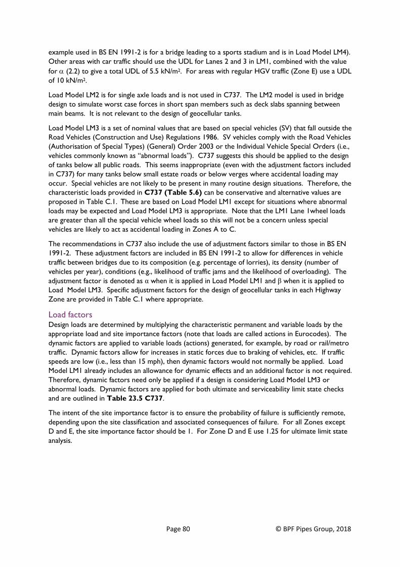
Page 80 © BPF Pipes Group, 2018
example used in BS EN 1991-2 is for a bridge leading to a sports stadium and is in Load Model LM4).
Other areas with car traffic should use the UDL for Lanes 2 and 3 in LM1, combined with the value
for (2.2) to give a total UDL of 5.5 kN/m2. For areas with regular HGV traffic (Zone E) use a UDL
of 10 kN/m2.
Load Model LM2 is for single axle loads and is not used in C737. The LM2 model is used in bridge
design to simulate worst case forces in short span members such as deck slabs spanning between
main beams. It is not relevant to the design of geocellular tanks.
Load Model LM3 is a set of nominal values that are based on special vehicles (SV) that fall outside the
Road Vehicles (Construction and Use) Regulations 1986. SV vehicles comply with the Road Vehicles
(Authorisation of Special Types) (General) Order 2003 or the Individual Vehicle Special Orders (i.e.,
vehicles commonly known as “abnormal loads”). C737 suggests this should be applied to the design
of tanks below all public roads. This seems inappropriate (even with the adjustment factors included
in C737) for many tanks below small estate roads or below verges where accidental loading may
occur. Special vehicles are not likely to be present in many routine design situations. Therefore, the
characteristic loads provided in C737 (Table 5.6) can be conservative and alternative values are
proposed in Table C.1. These are based on Load Model LM1 except for situations where abnormal
loads may be expected and Load Model LM3 is appropriate. Note that the LM1 Lane 1wheel loads
are greater than all the special vehicle wheel loads so this will not be a concern unless special
vehicles are likely to act as accidental loading in Zones A to C.
The recommendations in C737 also include the use of adjustment factors similar to those in BS EN
1991-2. These adjustment factors are included in BS EN 1991-2 to allow for differences in vehicle
traffic between bridges due to its composition (e.g. percentage of lorries), its density (number of
vehicles per year), conditions (e.g., likelihood of traffic jams and the likelihood of overloading). The
adjustment factor is denoted as α when it is applied in Load Model LM1 and β when it is applied to
Load Model LM3. Specific adjustment factors for the design of geocellular tanks in each Highway
Zone are provided in Table C.1 where appropriate.
Load factors Design loads are determined by multiplying the characteristic permanent and variable loads by the
appropriate load and site importance factors (note that loads are called actions in Eurocodes). The
dynamic factors are applied to variable loads (actions) generated, for example, by road or rail/metro
traffic. Dynamic factors allow for increases in static forces due to braking of vehicles, etc. If traffic
speeds are low (i.e., less than 15 mph), then dynamic factors would not normally be applied. Load
Model LM1 already includes an allowance for dynamic effects and an additional factor is not required.
Therefore, dynamic factors need only be applied if a design is considering Load Model LM3 or
abnormal loads. Dynamic factors are applied for both ultimate and serviceability limit state checks
and are outlined in Table 23.5 C737.
The intent of the site importance factor is to ensure the probability of failure is sufficiently remote,
depending upon the site classification and associated consequences of failure. For all Zones except
D and E, the site importance factor should be 1. For Zone D and E use 1.25 for ultimate limit state
analysis.

Page 81 © BPF Pipes Group, 2018
Table C.1 Suggested loads and adjustment factors
UDL
CharacteristicCIRIA
traffic
category
(pervious
surfaces)
CIR
IA C
737
des
crip
tio
n
Des
crip
tio
n f
or
hig
hw
ays
Hig
hw
ays
Zon
e
Typ
ical
veh
icle
s/lo
adin
g
Dis
trib
ute
d (
kN/m
2 )
ULS
wh
eel l
oad
Det
ails
Max
wh
eel l
oad
in m
od
el
(ap
plie
d p
ress
ure
at
surf
ace
- k
N/m
2 ) (h
alf
of
axle
load
)
Dyn
amic
am
plif
icat
ion
fact
or
-DA
F
Ove
rlo
ad f
acto
r
Ad
just
men
t fa
cto
r (
) to
allo
w f
or
low
er lo
ads
than
inte
rnat
ion
al H
GV
and
100
0-ye
ar r
etu
rn
per
iod
Ch
arac
teri
stic
wh
eel
load
at
gro
un
d s
urf
ace
(pre
ssu
re -
kN
/m2 )
Acc
iden
tal l
oad
Wh
eel
load
Det
ails
Max
wh
eel l
oad
in m
od
el
(ap
plie
d p
ress
ure
at
surf
ace
- k
N/m
2 ) (h
alf
of
axle
load
)
Dyn
amic
am
plif
icat
ion
fact
or
-DA
F
Ove
rlo
ad f
acto
r
Ad
just
men
t fa
cto
r (
) to
allo
w f
or
low
er lo
ads
than
inte
rnat
ion
al H
GV
and
100
0-ye
ar r
etu
rn
per
iod
Ch
arac
teri
stic
wh
eel
load
at
gro
un
d s
urf
ace
(pre
ssu
re -
kN
/m2 )
0
Small domestic gardens
(isolated from roads
and vehicle access)
Anywhere that vehicle
access is not possible
(e.g., due to fences or
barriers)
1
Small domestic gardens
(adjacent to drives or
roads)
N/A
2/3
Car park (with height or
width barriers to limit
access)
Anywhere that only
cars can access due to
physical constraints
e.g., width or height
barriers
B Car 5.5 LM1 Lane 3 100kN axle load
on 400mm by
400mm contact
area
313 1 1 1 313 LM1 Lane 3 100kN axle load
on 400mm by
400mm contact
area
313 1 1.5 1 470
4
Car parks without
barriers
Anywhere that HGVs
will only access as an
“accidental load” (i.e.,
not regular such as
vehicle overrun on a
verge at the back of a
footway)
C Mainly cars
with accidental
HGV loading
5.5 LM1 Lane 2
for "normal"
HGV
200kN axle load
on 400mm by
400mm contact
area
625 1 1 0.8 500 LM1 Lane 2 200kN axle load
on 400mm by
400mm contact
area
625 1 1 1 625
5
Private roads or cul-de-
sacs, access tracks
(<15mph)
Anywhere that is
subject to limited HGV
traffic at very low speed
such as fire tenders and
refuse trucks
D Cars and
"normal" HGV
at low speed
5.5 LM1 Lane 2 200kN axle load
on 400mm by
400mm contact
area
625 1 1 1 625 LM1 Lane 1 300kN axle load
on 0.4m by
0.4m contact
area (includes
DAF)
938 1 1 0.8 750
6
HGV parks, loading bays E1 Cars and
"normal" HGV
10 LM1 Lane 1
for "normal"
HGV
300kN axle load
on 0.4m by
0.4m contact
area (includes
DAF)
938 1 1 0.8 750 LM1 Lane 1 300kN axle load
on 0.4m by
0.4m contact
area (includes
DAF)
938 1 1 1 938
6
Public roads, estate
roads
E2 Cars and
"international"
HGV
10 LM1 Lane 1 300kN axle load
on 0.4m by
0.4m contact
area (includes
DAF)
938 1 1 1 938 LM1 Lane 1 300kN axle load
on 0.4m by
0.4m contact
area (includes
DAF)
938 1 1.2 1 1126
7+
Public highway (trunk
roads)
E3 Cars and
"international"
HGV plus
Special Vehicles
10 LM1 Lane 1 300kN axle load
on 0.4m by
0.4m contact
area (includes
DAF)
938 1 1.2 1 1126 LM1 Lane 1 300kN axle load
on 0.4m by
0.4m contact
area (includes
DAF)
938 1 1.5 1 1407
Note: Special vehicle loads give lower wheel loads than LM1 Lane 1
Consider risk of
trafficking
where adjacent
to drives or
roads and
possibly use
LM1 Lane 3
100kN axle load
on 400mm by
400mm contact
area
313 1 1 1 313
Everywhere else
(assumed to be subject
to regular unrestricted
HGV traffic)
Wheel Load Normal Service Load Case Wheel Load Accidental Load Case
A Pedestrian 2.5 (but
increase to 5 if
there is a risk of
crowds)
None - 0 - - - 0

Page 82 © BPF Pipes Group, 2018
Appendix D: Braking forces
C737 (5.3.4.3) indicates that horizontal braking forces may be transmitted to tanks. For routine
designs, the dynamic factor allowed for in the load models discussed above will be sufficient to allow
for this where units have a cover of 0.6 m or greater up to load Zone C (mainly cars) and over
1.0 m in all other cases.
C737 suggests that braking forces on the side of tanks should be determined in accordance with EC7
assuming that the braking force is 60% of the vertical load. This approach from bridge engineering is
over-conservative when applied to geocellular tanks that are at some depth below the application of
the wheel loads which dissipate through the adjacent and overlying pavement structure and soils
(Figure D.1 of this guidance). Horak et al5 demonstrated that the horizontal shear forces from heavy
aircraft braking and turning, such as a Boeing 747 “Jumbo Jet”, would be dissipated to a negligible
level within the top 100 mm of the pavement surface. Therefore, the preceding analysis, that takes
account of the horizontal component of the wheel load located adjacent to a tank, is sufficient to
allow for braking forces if vehicles drive onto a tank perpendicular to the edge. It is not considered
necessary to carry out an additional analysis as suggested by C737.
5 Horak E, Emery S, Maina J W and Walker B (2009). Mechanistic Modelling of Potential Interlayer Slip at Base Sub-base Level. Eighth International Conference on the Bearing Capacity of Roads, Railways, and Airfields, June 29 to July 2, 2009, University of Illinois, Urbana Champaign
Page 83 © BPF Pipes Group, 2018
Figure D.1 Comparison of braking forces on bridges and geocellular tanks

Page 84 © BPF Pipes Group, 2018
Appendix E: Lateral loads and arching
Introduction Historically, the design of geocellular tanks using the guidance provided in C680 has not explicitly
considered the effects of creep in the lateral design. There is some allowance for creep effects in
the design using short-term lateral strength and a factor of safety of 2.75 (along with yield strength
and tests in which failure takes at least 10 minutes). There is, however, no requirement in C680 for
a specific lateral creep assessment as there is for vertical loading.
The reason for this is because it is understood that the geocellular tanks are flexible and, therefore,
arching occurs in the soils to reduce the pressure on the side of the tank.
C737 has introduced a requirement to consider the lateral creep and it is apparent that using
maximum earth pressures estimated using traditional earth pressure theory (as used for retaining
walls) alongside long-term 50-year creep strength would significantly reduce the depths to which
current modules can be installed.
Therefore, an assessment of the likely reduction in earth pressure on the side of tanks due to
arching has been completed.
Evidence for arching effects
C737 identifies that arching can reduce the earth pressure applied to cells below the values
predicted by simple earth pressure theory (see Figure 2.39 C737).
The graph shows the horizontal stress on the cell for different cell stiffnesses. For a tank:soil
stiffness ratio of 0.5 MPa:8.6 MPa, i.e., 0.06, the maximum pressure in the tank is about 30% less than
the pressure with no tank6. The text states that arching has reduced the pressure to values below
the active pressure predicted by simple theory. As the stiffness of the tank increases, the earth
pressure on the side increases until (for very stiff units where the stiffness exceeds the soil stiffness
by a large amount) the earth pressure on the side of the tank is similar to the earth pressure with no
tank.
The two main factors that will affect whether arching can occur are the ratio of cover depth to tank
height and the ratio of tank lateral stiffness to soil stiffness (Figure E.1).
6 Typical values of Young’s Modulus for soil and granular material can be found in source document, Geotechdata.info, Soil Young’s Modulus, http://www.geotechdata.info/parameter/soil-young's-modulus.html, updated September 2013.

Page 85 © BPF Pipes Group, 2018
Figure E.1 Arching around a geocellular tank
The effect of lateral yielding of earth-retaining structures and the reduction in earth pressure is also
recognised in the design of reduced pressure retaining walls and bridge abutments. Polystyrene is
used as a flexible layer at the rear of walls and it can reduce earth pressure to below active values7.
Experience in the UK, Europe and Japan suggests that there is a significant difference between the
theoretical earth pressure estimated on the side of geocellular drainage tanks and that which occurs
in practice. The tanks are flexible buried structures and the soil structure interaction is complex
and, therefore, the analysis is not as straightforward as it would first appear. There has been very
little research in this area. However, BBA certificates in place for 10 years or so require
manufacturers to advise of any failures and there have been no lateral failures reported. What is
known is that the tanks have been used for over 20 years in Europe and Japan and there are very
few reported lateral failures, despite suggestions that the lateral strengths are insufficient for the
depths at which some are installed.
There are several possible reasons for the difference between simple theory and practice. The main
reasons that earth pressure is overestimated are:
• Relaxation of structure and arching within the soil.
• Conservatism in design parameters.
• Cohesive soils take time to reach fully-drained conditions with c’ = 0.
The usual method of estimating the earth pressure on the side of tanks is to adopt the approach
from conventional retaining wall analysis. This assumes a rigid wall that is free to rotate. A plastic
geocellular tank behaves differently to this and the reduced stiffness when compared to traditional
materials means that the soil:structure behaviour is such that lateral pressures are unlikely to ever
reach full active earth pressure. It also assumes that the only resistance to the applied forces is that
provided by the geocellular tank. Again, this is not always the case, especially where the depth of
cover soils is substantial. The cover soils can provide a significant amount of resistance against the
wedge of soil that is mobilized during development of lateral active earth pressures. An analogy is
the soil pressures on buried plastic pipes that are much lower than for rigid materials.
7 Koerner R M. Designing with Geosynthetics, 6th Edition, Volume 2, 2012
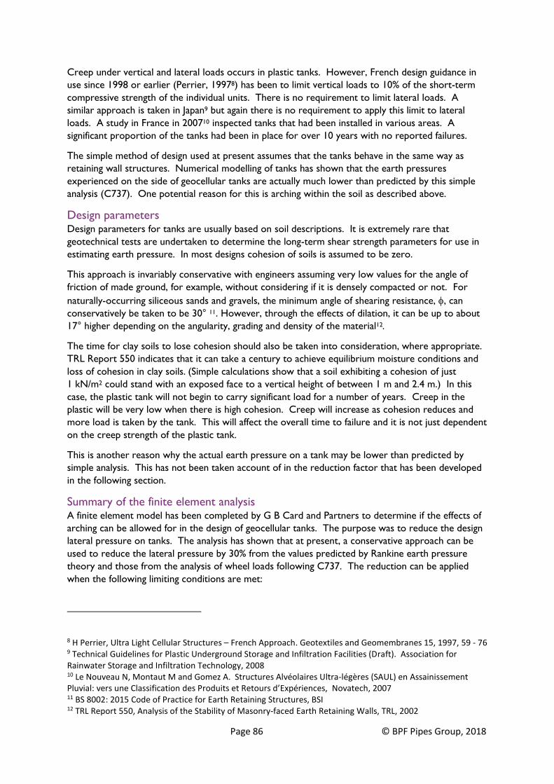
Page 86 © BPF Pipes Group, 2018
Creep under vertical and lateral loads occurs in plastic tanks. However, French design guidance in
use since 1998 or earlier (Perrier, 19978) has been to limit vertical loads to 10% of the short-term
compressive strength of the individual units. There is no requirement to limit lateral loads. A
similar approach is taken in Japan9 but again there is no requirement to apply this limit to lateral
loads. A study in France in 200710 inspected tanks that had been installed in various areas. A
significant proportion of the tanks had been in place for over 10 years with no reported failures.
The simple method of design used at present assumes that the tanks behave in the same way as
retaining wall structures. Numerical modelling of tanks has shown that the earth pressures
experienced on the side of geocellular tanks are actually much lower than predicted by this simple
analysis (C737). One potential reason for this is arching within the soil as described above.
Design parameters Design parameters for tanks are usually based on soil descriptions. It is extremely rare that
geotechnical tests are undertaken to determine the long-term shear strength parameters for use in
estimating earth pressure. In most designs cohesion of soils is assumed to be zero.
This approach is invariably conservative with engineers assuming very low values for the angle of
friction of made ground, for example, without considering if it is densely compacted or not. For
naturally-occurring siliceous sands and gravels, the minimum angle of shearing resistance, , can
conservatively be taken to be 30° 11. However, through the effects of dilation, it can be up to about
17° higher depending on the angularity, grading and density of the material12.
The time for clay soils to lose cohesion should also be taken into consideration, where appropriate.
TRL Report 550 indicates that it can take a century to achieve equilibrium moisture conditions and
loss of cohesion in clay soils. (Simple calculations show that a soil exhibiting a cohesion of just
1 kN/m2 could stand with an exposed face to a vertical height of between 1 m and 2.4 m.) In this
case, the plastic tank will not begin to carry significant load for a number of years. Creep in the
plastic will be very low when there is high cohesion. Creep will increase as cohesion reduces and
more load is taken by the tank. This will affect the overall time to failure and it is not just dependent
on the creep strength of the plastic tank.
This is another reason why the actual earth pressure on a tank may be lower than predicted by
simple analysis. This has not been taken account of in the reduction factor that has been developed
in the following section.
Summary of the finite element analysis A finite element model has been completed by G B Card and Partners to determine if the effects of
arching can be allowed for in the design of geocellular tanks. The purpose was to reduce the design
lateral pressure on tanks. The analysis has shown that at present, a conservative approach can be
used to reduce the lateral pressure by 30% from the values predicted by Rankine earth pressure
theory and those from the analysis of wheel loads following C737. The reduction can be applied
when the following limiting conditions are met:
8 H Perrier, Ultra Light Cellular Structures – French Approach. Geotextiles and Geomembranes 15, 1997, 59 - 76 9 Technical Guidelines for Plastic Underground Storage and Infiltration Facilities (Draft). Association for Rainwater Storage and Infiltration Technology, 2008 10 Le Nouveau N, Montaut M and Gomez A. Structures Alvéolaires Ultra-légères (SAUL) en Assainissement Pluvial: vers une Classification des Produits et Retours d’Expériences, Novatech, 2007 11 BS 8002: 2015 Code of Practice for Earth Retaining Structures, BSI 12 TRL Report 550, Analysis of the Stability of Masonry-faced Earth Retaining Walls, TRL, 2002

Page 87 © BPF Pipes Group, 2018
• The cover height to tank height ratio must be 0.48 or greater; and
• Soil to tank stiffness ratio must be 1.0 or greater.
Further refinement and verification of the finite element model may allow much greater reductions
to be applied in a wider range of conditions. Note that the reduction should only be applied to
earth pressure and not groundwater pressure.
The results are summarised in the Tables below.

Page 88 © BPF Pipes Group, 2018
Table E.1 Soft clay with UDL
0.6 m cover depth 1.0 m cover depth 2.0 m cover depth
Soft clay, 10 kPa UDL, = 17
kN/m2
Soft clay, 10 kPa UDL, =
17 kN/m2
Soft clay, 10 kPa UDL, =17 kN/m2
= 24°
Ka = TAN2(45 – /2) = 0.42
= 24o
= 24o
Rankine active earth pressure =
32.8 kPa (Red dotted line), (17 x
4 x 0.42) + (10 x 0.42)
Rankine active earth pressure =
32.8 kPa (Red dotted line)
Rankine active earth pressure =
32.8 kPa (Red dotted line)
In summary, for a soft clay for cover depths of 0.6 m and 1 m, the earth pressure at the mid-point of
the tank (horizontally) is effectively close to Rankine active pressure. When cover depth is 2 m, the
pressure on the side of the tank at 4 m is 21 kPa which is a reduction of 11.8 kPa (36%).

Page 89 © BPF Pipes Group, 2018
Table E.2 Soft clay with wheel load
0.6 m cover depth 1.0 m cover depth 2.0 m cover depth
Soft clay
Phi = 24°
Earth pressure from wheel load
C737 method = 14.78 kPa (Red
dotted line)
Earth pressure due to surcharge
from wheel load C737 method =
14.78 kPa (Red dotted line shows
total earth pressure)
Soft clay
Phi = 24°
Earth pressure due to surcharge
from wheel load C737 method =
14.78 kPa (Red dotted line shows
total earth pressure)
Soft clay
Phi = 24°
Earth pressure due to surcharge
from wheel load C737 method =
14.78 kPa (Red dotted line shows
total earth pressure)
In summary, the maximum lateral pressure from the wheel load occurs at shallow depth
(approximately 0.5 m) which is consistent with analysis in the BPF Pipes Group guide to C737. The
influence of the wheel load on lateral pressure below about 1.2 m cover depth is negligible. The
total pressure on the tank at 4 m depth is 27 kPa for 0.6 m cover, 29 kPa for 1 m and 18 kPa for 2 m
(38%, 33% and 58% reduction compared to values calculated using C737).
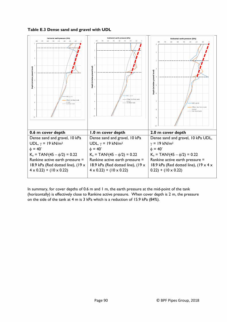
Page 90 © BPF Pipes Group, 2018
Table E.3 Dense sand and gravel with UDL
0.6 m cover depth 1.0 m cover depth 2.0 m cover depth
Dense sand and gravel, 10 kPa
UDL, = 19 kN/m2
Dense sand and gravel, 10 kPa
UDL, = 19 kN/m2
Dense sand and gravel, 10 kPa UDL,
= 19 kN/m2
= 40°
Ka = TAN2(45 – /2) = 0.22
= 40°
Ka = TAN2(45 – /2) = 0.22
= 40°
Ka = TAN2(45 – /2) = 0.22
Rankine active earth pressure =
18.9 kPa (Red dotted line), (19 x
4 x 0.22) + (10 x 0.22)
Rankine active earth pressure =
18.9 kPa (Red dotted line), (19 x
4 x 0.22) + (10 x 0.22)
Rankine active earth pressure =
18.9 kPa (Red dotted line), (19 x 4 x
0.22) + (10 x 0.22)
In summary, for cover depths of 0.6 m and 1 m, the earth pressure at the mid-point of the tank
(horizontally) is effectively close to Rankine active pressure. When cover depth is 2 m, the pressure
on the side of the tank at 4 m is 3 kPa which is a reduction of 15.9 kPa (84%).

Page 91 © BPF Pipes Group, 2018
Table E.4 Dense sand and gravel with wheel load
0.6 m cover depth 1.0 m cover depth 2.0 m cover depth
Dense sand and gravel, wheel
load
= 40°
Earth pressure due to surcharge
from wheel load C737 method =
7.7 kPa (Red dotted line shows
total earth pressure)
Dense sand and gravel, wheel
load
= 40°
Earth pressure due to surcharge
from wheel load C737 method =
7.7 kPa (Red dotted line shows
total earth pressure)
Dense sand and gravel, wheel
load
= 40°
Earth pressure due to surcharge
from wheel load C737 method
= 7.7 kPa (Red dotted line
shows total earth pressure)
In summary, for dense sand gravel the maximum lateral pressure from the wheel load occurs at
shallow depth (approximately 0.5 m) which is consistent with analysis in the BPF Pipes Group guide
to C737. With 2 m cover, the peak load remains to 2 m depth and it is not clear why this is the
case, although it makes no difference to the outcome of this assessment. The influence of the wheel
load on lateral pressure below 2 m cover depth is negligible. The total pressure on the tank at 4 m
depth is 3 kPa for 0.6 m cover and 2 m cover (88% reduction compared to values calculated using
C737). The analysis suggests that there is a slight increase in lateral pressure for the 1m cover. This
is not consistent with the other two analyses and is not considered representative in this
assessment.

Page 92 © BPF Pipes Group, 2018
Ground truthing the model The model has been compared to a trial installation that was completed at a site. The lateral
movement of the tank was measured. The actual movement has been compared to that predicted
by this finite element model.
Figure E.2 Comparison of predicted with actual movements
The measured deflections are lower than predicted with the soil backfill but are higher than
predicted with the water pressure. These differences are likely due to the assumptions on soil
properties made in the model. The variations in deflected profile are due to the simplifying
assumptions on the lateral stiffness in the model. A uniform stiffness is assumed when in practice
parts of the tank are stiffer than others. However, the results indicate a generally positive
correlation between the model and the trial.
The earth pressure 5 m from the tank and below the base also fits well with the theoretical values.
Conclusions For any tank/soil stiffness ratio, if the cover to tank height ratio is less than 0.5, there is no reduction
in pressure for UDL. For cover to tank height ratio of 0.5 or greater, the lateral earth pressure with
a UDL can be reduced by 36% from that predicted by the Rankine approach.
With a wheel load and dense sand and gravel, the maximum pressure on a tank with a wheel load
can be reduced by 88%. For soft clay it can be reduced by 33%.
To derive reduction factors for use in routine design, a conservative approach has been adopted
from the above analysis. For simplicity and to allow for some of the inconsistency in the results,
assume a 30% reduction from Rankine or C737 wheel pressure across all analyses where the ratio
of cover depth to tank height exceeds 0.48 (see graphs below in Figures E.3 and E.4) and soil to tank
stiffness ratio is greater than 1. This cover must be maintained below any services that cross the
tank and measures should be put in place to prevent accidental excavation that would impair the
arching effect.
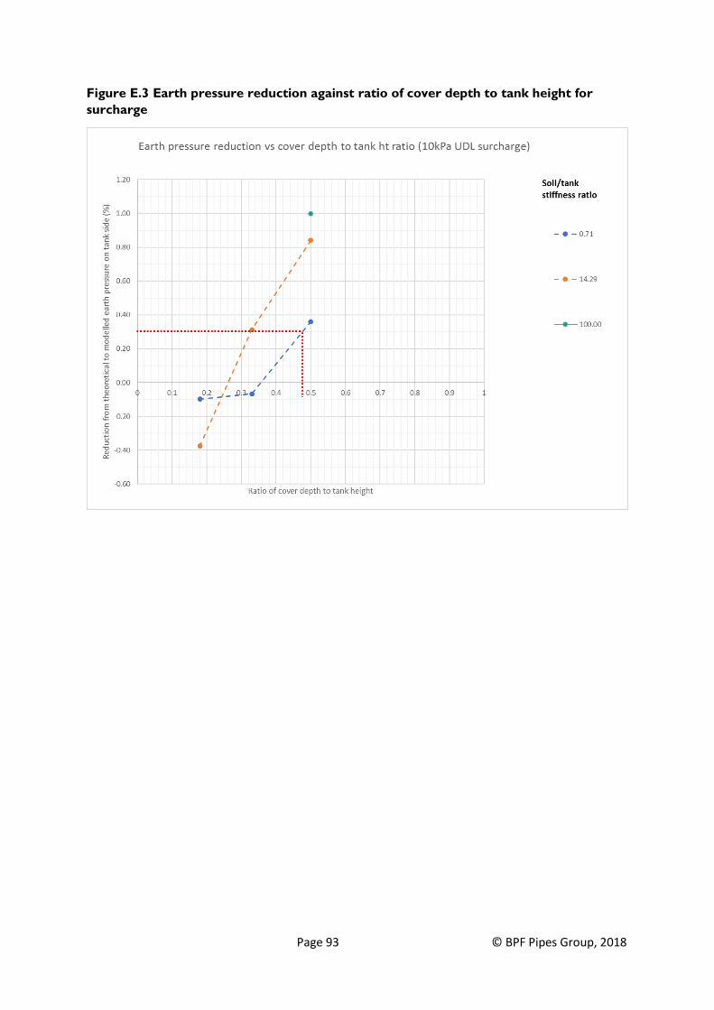
Page 93 © BPF Pipes Group, 2018
Figure E.3 Earth pressure reduction against ratio of cover depth to tank height for
surcharge

Page 94 © BPF Pipes Group, 2018
Figure E.4 Earth pressure reduction vs depth:tank height for wheel loads
Using a reduction factor to allow for arching may not be applicable where excavations for tanks are
within the global critical shear surface for adjacent slopes or foundations. Arching effects apply only
to soil and traffic loads and not to groundwater pressure.
With further modelling and verification of the model against field data, the graphs above could be
refined.
The 30% reduction is consistent with the example in Figure 2.39 of C737 (although the cover
depth ratio for that example is not known). It is also consistent with the reduction in earth pressure
on retaining walls using geofoam as reported by Koerner (2012)7.
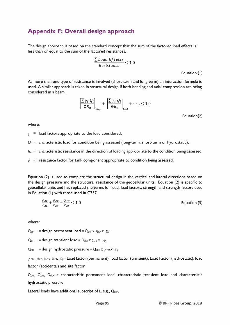
Page 95 © BPF Pipes Group, 2018
Appendix F: Overall design approach
The design approach is based on the standard concept that the sum of the factored load effects is
less than or equal to the sum of the factored resistances.
∑ 𝐿𝑜𝑎𝑑 𝐸𝑓𝑓𝑒𝑐𝑡𝑠
𝑅𝑒𝑠𝑖𝑠𝑡𝑎𝑛𝑐𝑒≤ 1.0
Equation (1)
As more than one type of resistance is involved (short-term and long-term) an interaction formula is
used. A similar approach is taken in structural design if both bending and axial compression are being
considered in a beam.
[∑ 𝛾𝑖 𝑄𝑖
∅𝑅𝑛]
𝐿𝑆1
+ [∑ 𝛾𝑖 𝑄𝑖
∅𝑅𝑛]
𝐿𝑆2
+ ⋯ . . ≤ 1.0
Equation(2)
where:
i = load factors appropriate to the load considered;
Qi = characteristic load for condition being assessed (long-term, short-term or hydrostatic);
Rn = characteristic resistance in the direction of loading appropriate to the condition being assessed;
ϕ = resistance factor for tank component appropriate to condition being assessed.
Equation (2) is used to complete the structural design in the vertical and lateral directions based on
the design pressure and the structural resistance of the geocellular units. Equation (2) is specific to
geocellular units and has replaced the terms for load, load factors, strength and strength factors used
in Equation (1) with those used in C737.
𝑄𝑑𝑃
𝑃𝑑𝐿+
𝑄𝑑𝑇
𝑃𝑑𝑆+
𝑄𝑑𝐻
𝑃𝑑𝐿≤ 1.0 Equation (3)
where:
QdP = design permanent load = QckP x LFP x sf
QdT = design transient load = QckT x LFT x sf
QdH = design hydrostatic pressure = QckH x LFH x sf
LFP, LFT, LFHLFAsf = Load factor (permanent), load factor (transient), Load Factor (hydrostatic), load
factor (accidental) and site factor
QckP, QckT, QckH = characteristic permanent load, characteristic transient load and characteristic
hydrostatic pressure
Lateral loads have additional subscript of L, e.g., QckPL

Page 96 © BPF Pipes Group, 2018
PdL = Design characteristic long-term creep resistance from module tests = long-term creep
resistance from module tests in the direction of loading appropriate to the design life, PckL x mL
PdS = Design short-term yield resistance from tests = characteristic short-term yield resistance from
tests in the direction of loading, PckS x mS
Lateral strengths have additional subscript of L, e.g., PckLL
mL, mS = resistance factor for tank component

Page 97 © BPF Pipes Group, 2018
Appendix G: Determining yield strength from short-term
tests – the BBA approach
BBA have adopted the principle of determining the yield strength of units from short-term test data
as follows:
1. Plot the load vs deflection on a graph (as shown in Figure G.1 below).
2. Ignore the seating part of the curve and any data beyond the peak failure load to determine
the number of data points.
3. Locate the points on the load/deflection curve that correspond to 10% and 40% of the data
points and draw a line between them – in the example below, that is the line with the
equation y = 4.1636x + 5.2168. This is the trend in the elastic range.
4. Locate the points on the load/deflection curve that correspond to 90% and 100% of the data
points and draw a line between them – in the example below, that is the line with the
equation y = 0.3503x + 30.855. This is the trend in the plastic range.
5. The intersection of the two lines gives the yield strength – in the example below yield
strength = 34kN.
Figure G.1 Example estimation of yield strength


